3rd International Workshop on Human Error, Safety, and System Development, Liège, Belgium, June 7-8, 1999

Integrating Objective and Subjective Hazard Risk in Decision-Aiding System Design

Deborah S. Hyams, David M. Matsumoto, and James K. Kuchar

Department of Aeronautics and Astronautics

Massachusetts Institute of Technology Cambridge, MA 02139 USA

Abstract A generalized model is presented to incorporate objective (hard) and subjective (soft) hazard

information in automated decision-aiding systems. The model may be used with more than one hazard, of more than one type, in a given problem. Uncertainties in state measurements, dynamics, hazard extent, and hazard severity are included, as is consideration of the fact that different operators may have different concepts of what is an acceptable or unacceptable risk. By examining the tradeoffs created by these uncertainties, appropriate decision thresholds can be selected. Using an aviation case study, information gained from observation of aircraft behavior in the presence of weather was used to develop a model of weather as a soft hazard. This information could then be used in a decision aid to provide feedback on route acceptability.

Introduction Real-time decision aiding and alerting systems are often used to assist human operators in

controlling processes efficiently and in preventing undesirable incidents from occurring (such as a collision in a vehicle control application, or exceeding temperature limits in process control). There are a number of types of real-time decision aids, ranging from process status displays, to planning tools, to safety- and time-critical warning systems. However, all decision aids can be broadly classified as either active or passive. Active systems generate discrete decisions or commands that are communicated to the operator with the intent of modifying the process’ future state trajectory (e.g., a traffic conflict resolution command). Passive systems provide process and environment state information to the operator (e.g., depicting precipitation levels on a weather radar display) without explicit decisions being made by the automation. Thus, an active system acts as an automated decision maker (which may agree or disagree with the human operator’s decisions), while a passive system acts as an automated decision supporter.

To date, the use of active systems has generally been restricted to cases in which there is a clear definition of hazardous states. For example, traffic collision risk can be defined in concrete, objective terms (e.g., no closer than 500 ft separation between aircraft), which then is translated into algorithms and decision thresholds. This can be classified as a case of objective assessment of hazard risk. Due to sensor and prediction errors, there still may be uncertainty in whether a decision to change the process’ trajectory is needed. These uncertainties, however, can also be objectively estimated and used when defining decision thresholds to balance false alarms and missed detections and optimize system performance from the human operator’s perspective.

In cases in which the distinction between hazard and non-hazard is less distinct (i.e., the hazard risk is subjective), decision aids typically display the state information but leave the

1

decision making to the human operator. Aviation examples of subjective hazards include weather precipitation levels, turbulence intensities, forecast icing, or visibility.

For an automation tool to be accepted, the decisions and feedback it provides should be aligned with operator mental models and expectations. A decision aid that does not consider subjective hazards may generate inappropriate decisions that decrease operator confidence and acceptance. For example, several automation tools are being developed for detecting and resolving air traffic conflicts and managing the arrival flow at airports (Davis et al., 1994; Slattery & Green, 1994; Paielli & Erzberger, 1997). These tools currently do not include hazardous weather information in their automated decisions, though some study of incorporating weather has begun in this area (e.g., Krozel et al., 1997). When weather is not considered by the automation, the human operator must mentally integrate the information to determine whether a given automated suggestion is appropriate. This may increase workload and decrease the utility of the automation in poor weather conditions. There is an opportunity, then, to enhance the automation by including subjective information in its decision-making process. If an accurate model of subjective hazards cannot be developed, however, it may be more effective to have the operator perform this integration between objective and subjective hazards.

At issue, then, is whether automated decisions should be constrained to only objective hazard information, leaving the human to integrate the automation’s decision with other subjective hazard information, or whether some subjective information could be inserted into the automation’s decision-making process to reduce the human’s need to integrate. This paper describes a general modeling approach which integrates subjective and objective hazard risk into a form that can be used in an automated decision aid. An examination of the utility of this integrated active decision aid in different situations will be the subject of future research.

The method involves obtaining observations of human behavior in the presence of subjective hazards, translating this behavior into objective terms, and developing algorithms that then integrate the subjective hazard risk with objective hazard risk in an active decision aid. The result is an automated system that incorporates information about multiple hazard sources, both subjective (e.g., weather) and objective (e.g., traffic and terrain), into a trajectory planning decision. This paper outlines different methods for integrating this information, and describes a specific example application in which precipitation intensity information was used to develop a model of weather that can be integrated with other hazard information.

General model The class of decision-aiding problems considered in this paper involves those that can be

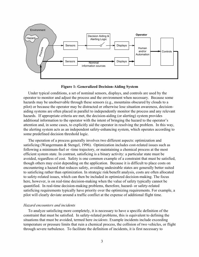
modeled in the framework in Figure 1. As shown, a process of interest is controlled through a combination of humans and automation in an environment in which undesirable hazardous states may exist. The operator’s task is to control the process to arrive at some desired end state without experiencing an undesirable incident. Example processes may include chemical or power processes, single vehicles, large-scale transportation systems, financial markets, or other applications. The operator may be a single human or a combination of automation and humans (e.g., in air traffic control several ground-based human controllers with automation aids may be managing a number of aircraft, each with several crew members and associated cockpit automation).

2

Environment

Decision Aiding & Alerting Logic

Proc

ess

ControlsHuman and/or

Automation

Nominal information sources

Sensors Displays

DisplaysSensors

HazardOperator

Figure 1: Generalized Decision-Aiding System

Under typical conditions, a set of nominal sensors, displays, and controls are used by the operator to monitor and adjust the process and the environment when necessary. Because some hazards may be unobservable through these sensors (e.g., mountains obscured by clouds to a pilot) or because the operator may be distracted or otherwise lose situation awareness, decision-aiding systems are often placed in parallel to independently monitor the process and any relevant hazards. If appropriate criteria are met, the decision-aiding (or alerting) system provides additional information to the operator with the intent of bringing the hazard to the operator’s attention and, in some cases, to explicitly aid the operator in resolving the problem. In this way, the alerting system acts as an independent safety-enhancing system, which operates according to some predefined decision threshold logic.

The operation of a process generally involves two different aspects: optimization and satisficing (Wangermann & Stengel, 1996). Optimization includes cost-related issues such as following a minimum-fuel or -time trajectory, or maintaining a chemical process at the most efficient system state. In contrast, satisficing is a binary activity: a particular state must be avoided, regardless of cost. Safety is one common example of a constraint that must be satisfied, though others may exist depending on the application. Because it is difficult to place costs on encountering a hazard that reduces safety, avoiding undesirable states are generally better suited to satisficing rather than optimization. In strategic risk/benefit analysis, costs are often allocated to safety-related issues, which can then be included in optimized decision-making. The focus here, however, is on real-time decision-making when the value of safety typically cannot be quantified. In real-time decision-making problems, therefore, hazard- or safety-related satisficing requirements typically have priority over the optimizing requirements. For example, a pilot will clearly deviate around a traffic conflict at the expense of additional flight time.

Hazard encounters and incidents To analyze satisficing more completely, it is necessary to have a specific definition of the

constraint that must be satisfied. In safety-related problems, this is equivalent to defining the situations that must be avoided, termed here incidents. Example incidents include exceeding temperature or pressure limits that ruin a chemical process, the collision of two vehicles, or flight through severe turbulence. To facilitate the definition of incidents, it is first necessary to

3

consider the process and environment in a state-space model. The appropriate choice of states depends on the application: in a vehicle control case, states could include position, velocity, and acceleration; in process control, states could include temperature, pressure, valve positions, and flow rates.

Because the occurrence of an incident may be a probabilistic event (e.g., flight through a region of heavy precipitation may involve severe turbulence, but it may not), the region in state space in which an incident is possible is partitioned and is termed Hazard Space (Figure 2). Thus, entry into Hazard Space (termed a hazard encounter) is necessary but not sufficient for an incident to occur. The problem then reduces to one of determining whether Hazard Space will be encountered during the operation of the process, and if so, the likelihood that an incident will then result. Trajectories that do not penetrate Hazard Space can then be optimized to meet other constraints such as time, fuel burn, or other metrics of efficiency.

Process State State Trajectory

Hazard Space

Figure 2: Process State, Trajectory, and Hazard Space

The definition of Hazard Space (and therefore the definition of an incident) can be tailored to meet the particular problem under study. For example, Hazard Space could be defined as the collision of two aircraft, as a near-miss event when aircraft are 500 ft apart, or as the loss of standard 5 nmi separation.

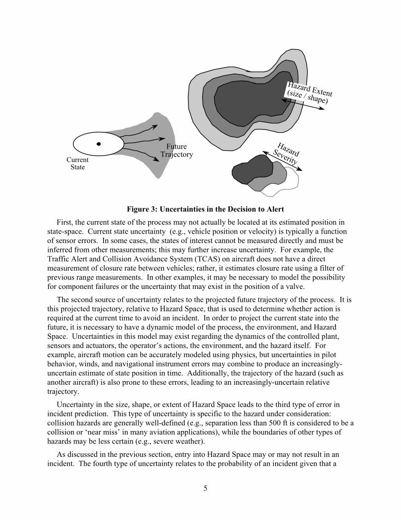
Uncertainties With perfect information, entry into Hazard Space can be predicted exactly. Generally,

however, this is not possible, due to the combination of four types of uncertainties. These uncertainties (current state, trajectory, extent, and severity) are shown schematically in Figure 3 and discussed in more detail below.

4

Current State

Hazard Severity

Hazard Extent (size / shape)

Future Trajectory

Figure 3: Uncertainties in the Decision to Alert

First, the current state of the process may not actually be located at its estimated position in state-space. Current state uncertainty (e.g., vehicle position or velocity) is typically a function of sensor errors. In some cases, the states of interest cannot be measured directly and must be inferred from other measurements; this may further increase uncertainty. For example, the Traffic Alert and Collision Avoidance System (TCAS) on aircraft does not have a direct measurement of closure rate between vehicles; rather, it estimates closure rate using a filter of previous range measurements. In other examples, it may be necessary to model the possibility for component failures or the uncertainty that may exist in the position of a valve.

The second source of uncertainty relates to the projected future trajectory of the process. It is this projected trajectory, relative to Hazard Space, that is used to determine whether action is required at the current time to avoid an incident. In order to project the current state into the future, it is necessary to have a dynamic model of the process, the environment, and Hazard Space. Uncertainties in this model may exist regarding the dynamics of the controlled plant, sensors and actuators, the operator’s actions, the environment, and the hazard itself. For example, aircraft motion can be accurately modeled using physics, but uncertainties in pilot behavior, winds, and navigational instrument errors may combine to produce an increasingly-uncertain estimate of state position in time. Additionally, the trajectory of the hazard (such as another aircraft) is also prone to these errors, leading to an increasingly-uncertain relative trajectory.

Uncertainty in the size, shape, or extent of Hazard Space leads to the third type of error in incident prediction. This type of uncertainty is specific to the hazard under consideration: collision hazards are generally well-defined (e.g., separation less than 500 ft is considered to be a collision or ‘near miss’ in many aviation applications), while the boundaries of other types of hazards may be less certain (e.g., severe weather).

As discussed in the previous section, entry into Hazard Space may or may not result in an incident. The fourth type of uncertainty relates to the probability of an incident given that a

5

hazard encounter has occurred. This can be thought of as a combination of an objective uncertainty in the severity of the hazard, and a subjective uncertainty in the definition of an incident. In the former, objective case, the structure of the hazard may be such that an incident occurs probabilistically following a hazard encounter: the hazard may be modeled using varying levels of “hardness” or “softness”. One example is flight over a missile site which might have been destroyed previously; whether or not a missile is launched can then be considered as a probabilistic event. While the estimation of this probability requires judgment, the threat posed by a missile launch could be considered objectively. Another example is the potential for component failure when operating outside a safe envelope.

In the latter, subjective uncertainty case, there may be differing opinion on what the proper definition of an incident is. Flight through poor weather, for example, may be acceptable to some operators and not to others. This acceptability is likely a function of many other factors such as operator experience and training, risk aversion or acceptance, the existence of alternate options, and the expected amount of time that will be spent in Hazard Space.

Decision Tradeoffs With hazards involving some uncertainty, any discrete decision to alert the operator or to

otherwise determine whether a given trajectory is acceptable may be in error in one of two ways. First, it may be the case that an alert was not necessary (termed an unnecessary alert). Alternately, it may be the case that the decision to alert is never made or is made too late to prevent an incident (a missed or late alert). The tradeoff between these outcomes is a critical factor in designing an acceptable decision-aiding system and has been examined previously for objective hazards (Kuchar, 1996).

When dealing with cases in which the definition of an incident is subjective, an additional form of decision tradeoff occurs. Consider a case in which it is known with certainty that the process will enter a soft hazard (that is, a hazard in which an encounter does not necessarily mean that an incident will occur). A decision to alert the operator may be an error if the operator does not consider the hazard sufficiently threatening. An analog to a missed detection may instead occur if an alert is not made, but the operator would have desired an alert. This is not to say that an alerting system must always match an operator’s mental model of when alerts should be issued — in some cases the operator may have an incomplete concept of whether action is truly required. However, studies have shown the importance of designing systems to provide feedback so that operators can understand the reasoning or logic behind an automated decision (Pritchett, 1996).

While the decision tradeoff with an objective definition of an incident can be examined using models of dynamics and uncertainties, subjective incidents may require additional consideration of human factors, expert opinion, and operational experience. In some cases, it may be desirable to have operator-selectable or situation-dependent thresholds that can be tuned to the particular problem at hand. As one example, the threat posed by weather varies significantly depending on aircraft type, pilot experience, and other environmental factors such as overall extent of the storm, proximity to terrain, or the availability of escape routes. A study by MIT Lincoln Laboratory, for example, found that pilots were significantly more likely to penetrate severe weather as they approached the runway, possibly due to pressures of the constrained

6

environment and to knowledge of the relatively short distance remaining to be flown (Rhoda & Pawlak, 1998).

The basic problem is then one in which at the current time, the alerting system must choose between alerting the operator to the hazard, or remaining silent and monitoring the situation. Alternatively, in non-alerting applications a decision-aiding system needs to provide feedback to the operator as to whether a given control strategy or trajectory is acceptable. These choices depend on whether an incident will occur along the projected nominal trajectory and also on the existence of acceptable options, should action need to be taken. The four types of uncertainty outlined above combine together, with the result that whether an incident will occur can only be estimated with some probability. The following section develops a formal method for computing this probability, including an example problem. The remainder of the paper then discusses issues in hazard modeling for an aviation weather case study.

Computation of Probability of Incident This section develops a formal, generic framework for modeling hazard situations and

computing the probability of an incident. In order to have a quantitative approach to analyze decision-making, it is necessary to model the dynamics of a hazard situation. The methodology abstracts the problem to state space and places the observable states relating to the process and any hazards in a vector, x(t).

It is appropriate at this point to recall the definitions of several events that affect decision-making. An incident, denoted I, is an event that the operator must avoid. Because different operators may have different thresholds of acceptability, this definition itself may be uncertain. Hazard Space is that subset of state-space in which an incident could occur, and a hazard encounter, E, is an event in which the system state vector x(t) lies within Hazard Space.

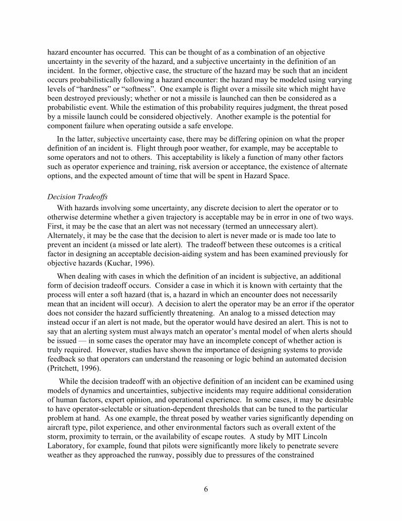
State-space model Figure 4 depicts an example state estimate, x , that includes some uncertainty (the dependence

on time is assumed implicitly from this point on). An error ellipse is shown in Figure 4 that describes the region in state-space in which x truly lies with some probability. Hazard Space, denoting a region where an incident can occur, is also shown.

ˆ

7

Unc

erta

inty

in

Futu

re T

raje

ctor

y (s

et T

)

Uncertainty in Current State Estimate

x 1

x 2

τ

x

Hazard Space

Figure 4: State-Space Diagram

Based on x , the alerting system must determine whether an alert is warranted. The need for an alert, however, depends on the trajectory that will be followed in the future. In Figure 4, one possible trajectory is denoted τ. The actual trajectory that will be followed, however, may be any within some set T of trajectories. T is probabilistic, and depends on uncertainties in x , future control inputs, and knowledge of the system dynamics. A shaded area is shown in Figure 4 that denotes the region where the true trajectory will be with some probability.

ˆ

ˆ

Having defined T, and given a particular state estimate, x , there exists some probability that an incident will occur in the future, denoted PT(I | x ). This notation explicitly shows that the probability is evaluated along the probabilistic trajectory T and is a function of x . As discussed earlier, PT(I | x ) is a function of uncertainties in the current state, future trajectory, hazard extent, and hazard severity.

ˆ ˆ

ˆ ˆ

Whether the decision-aiding system needs to alert the operator at the time shown in Figure 4 depends on the value of PT(I | x ). In general, the larger the probability that an incident will occur, the greater the need for an alert. An alert that is issued when PT(I | x ) is small may be considered a false alarm if the human operator is aware of the hazard or would have avoided the hazard without the alert. However, if the alert is delayed until PT(I | x ) is large, there may not be enough time or space in which to perform an avoidance maneuver and an incident may occur even if an alert is issued. A methodology to observe this tradeoff has been previously developed (Kuchar, 1996). In it, the probability of an incident along a particular trajectory is estimated through Monte Carlo simulation, numerical integration, or analytic methods (e.g., Kuchar & Carpenter, 1997; Paielli & Erzberger, 1997; Yang & Kuchar, 1997).

ˆ ˆ

ˆ

As discussed earlier, an encounter with Hazard Space (event E) is necessary but not sufficient for an incident (event I) to occur. Accordingly, PT(E | x ) is defined as the probability that a hazard encounter occurs along a particular uncertain trajectory T, and P

ˆ T(I | x ) is defined as the

probability that an incident occurs in that same situation. From Bayes’ Rule, ˆ

PT(I | x ) = P(I | E) Pˆ T(E | x ) (1) ˆ

Hazards for which P(I | E) = 1 are hard hazards. An encounter with a hard hazard means that an incident also occurs. An example hard hazard is a collision with another vehicle. Hazards for

8

which P(I | E) < 1 are soft hazards — an encounter does not necessarily indicate that an incident will also occur. Soft hazards include severe weather or safety thresholds beyond which component failures may occur. Methods for modeling hard and soft hazards are discussed in a following section.

Probability of Hazard Encounter, PT(E | ˆ x ) To estimate PT(I | x ), it is first necessary to calculate the probability that the process will

encounter Hazard Space along a probabilistic trajectory: PT(E | x ). As described earlier, a state estimate, x , is available but due to measurement errors the state may actually be located at a different position, x. The probability that the state is truly at some value x is given by the Probability Density Function (PDF)

ˆ ˆ

ˆ

ƒx (x − ˆ x ) and is typically based on sensor error distributions.

Assume initially that the process’ future trajectory, denoted by the vector τ, and the size and shape of Hazard Space (or hazard extent), denoted by the vector σ, are known perfectly a priori. Having defined these parameters, the probability that the process will encounter Hazard Space along the known trajectory τ in a situation with the given hazard extent σ and the current state estimate, x , is denoted as Pˆ T (E | ˆ x ,σ ,τ ) .

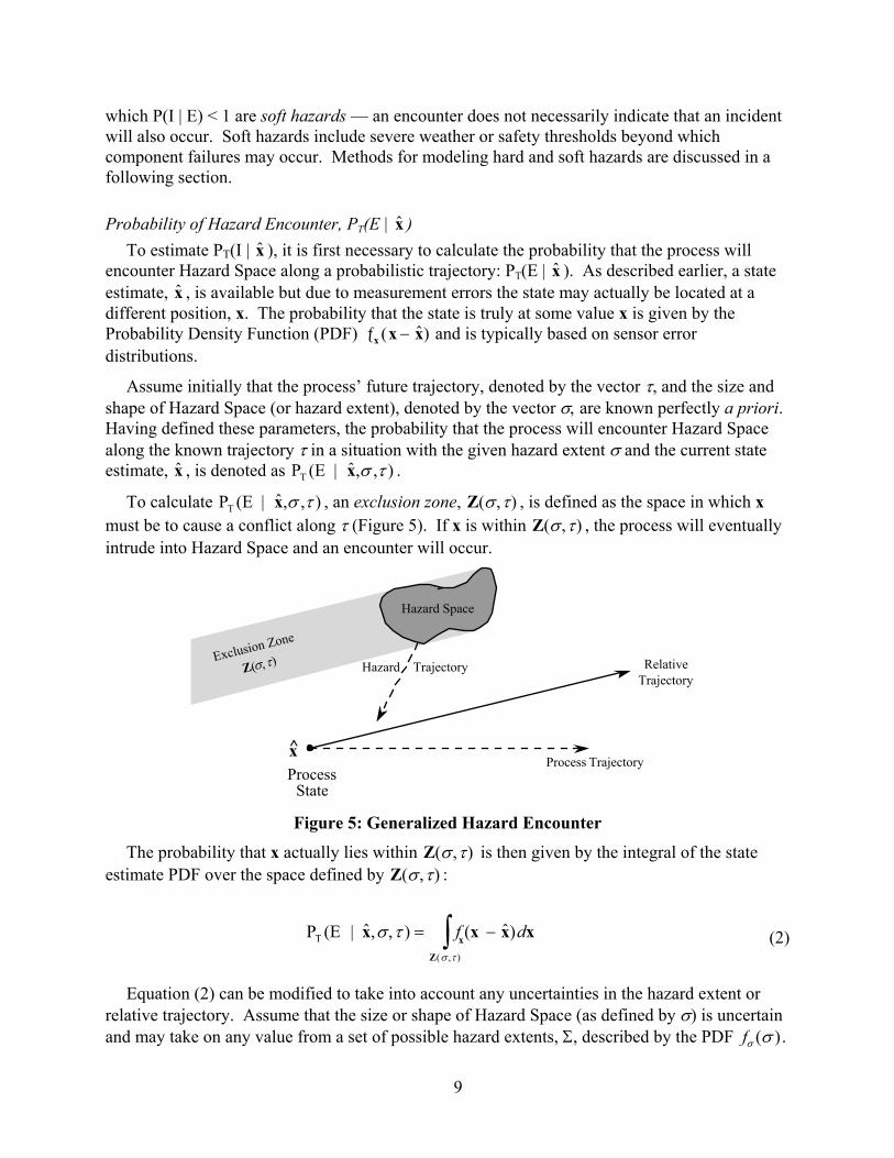
To calculate PT (E | ˆ x ,σ ,τ ) , an exclusion zone, Z(σ,τ) , is defined as the space in which x must be to cause a conflict along τ (Figure 5). If x is within Z(σ,τ) , the process will eventually intrude into Hazard Space and an encounter will occur.

Process Trajectory

Relative Trajectory

Hazard Trajectory

Process State

Exclusion Zone

Z(σ,τ)

x

Hazard Space

Figure 5: Generalized Hazard Encounter

The probability that x actually lies within Z(σ,τ) is then given by the integral of the state estimate PDF over the space defined by Z(σ,τ) :

PT (E | ˆ x ,σ,τ ) = fx(x − ˆ x )dxZ(σ ,τ )∫ (2)

Equation (2) can be modified to take into account any uncertainties in the hazard extent or relative trajectory. Assume that the size or shape of Hazard Space (as defined by σ) is uncertain and may take on any value from a set of possible hazard extents, Σ, described by the PDF fσ (σ ).

9

Assume also that τ can take on any value from a set of possible trajectories, T. The PDF fτ (τ ) describes the probability that any particular trajectory occurs, and is typically based on uncertainties in the dynamics of the situation, reaction time, and operator actions. The probability that an encounter will occur is then given by integrating Equation (2) over all possible values of σ and τ :

PT (E | ˆ x ) = fx (x − ˆ x ) fσ (σ ) fτ (τ ) dx dσ dτZ(σ ,τ )∫

Σ∫

T∫ (3)

Provided that the PDFs are known or can be estimated, this expression can be solved using numerical integration or Monte Carlo methods. Finally, P(I | E) is used [Equation (1)] to determine the probability of an incident, PT(I | x ). ˆ

Hazard Modeling In cases where an encounter with Hazard Space is the same as an incident (hard hazards),

and equation (3) is itself the probability of such an incident occurring: P(I | E) = 1

PT(I | x )ˆ hard = PT(E | x ) (4) ˆ

When an encounter with a hazard does not necessarily mean that an incident will occur (a soft hazard), the methodology must be further modified to account for P . There are two main approaches that can be taken to include soft hazards in the estimation of P

(I | E) <1T(I | x ). In the

first, only those hazards above some threshold level of severity are included in the computations of P

ˆ

T(I | ), and all such included hazards are treated equally: ˆ x

P(I | E) =0, if P(I | E) < threshold1, if P(I | E) ≥ threshold

(5)

Because a specific definition of the severity threshold is required, important threats that are just below the threshold may be missed, or threats just above the threshold might be considered to be more significant than they actually are. In an aviation example, the thresholding method might mean including aircraft and terrain collision threats and high-severity weather in the decision-making process, but neglecting areas of moderate or minor precipitation. Then, the general regions which should be avoided can be identified, but the specific nature of each hazard (traffic, terrain, or weather) may not be observable. This approach has the benefit of simplicity to the operator, but there may be a need to differentiate between each type of hazard when making decisions.

In the second approach, all hazards are included in the decision-making process, which weighs them according to their severity level, P(I | E). Only after computing PT(I | x ) is a discrete thresholded decision made to alert the operator. This has the benefit of carrying through as much information as possible, but is more computationally intensive.

ˆ

The probability of incident for soft hazards may be modeled in two ways. In the first, P(I | E) is independent of exposure (termed an exposure-time independent hazard). An example of an

10

exposure-independent hazard that has already been mentioned is a missile site that has a certain probability of being active on a particular day, regardless of how long the aircraft flies near it. The second model is one in which the probability of an incident depends on the time or distance over which an encounter occurs (termed an exposure-time dependent hazard). An example is hazardous weather — the longer an aircraft remains inside a thunderstorm, the greater the probability that an incident will occur.

When a soft exposure-time independent hazard is encountered, P(I | E) is less than 1. Assuming that this probability is constant over Hazard Space, PT(I | x ) can be determined using equation (1).

ˆ

When dealing with exposure-time dependent hazards, P(I | E) depends on the amount of time or distance that the trajectory remains in Hazard Space. The total exposure to the hazard along each possible trajectory is needed to calculate PT(I | x ). This exposure can be estimated by integrating a hazard severity density function,

ˆ fL(l), over the length of the trajectory through the

hazard:

P(I | E) = fL(l)dlτ∫ (6)

where l is the accumulated position along the trajectory inside the hazard.

For a constant-density threat, fL(l) can be modeled using an exponential distribution. For this purpose, the parameter θ is defined to represent an estimate of the mean amount of exposure (in units of distance or time) until an incident occurs. For example, a severe weather hazard that is modeled as having a mean time to an incident of θ = 10 min implies that, on average, a hazard encounter will result in an incident after flying for 10 minutes through the hazard. As θ tends toward zero, the hazard becomes more like a hard hazard — very small exposures result in incidents. A large value of θ indicates an insubstantial hazard to which a large exposure is required before an incident will likely occur. If θ is constant over the extent of the hazard, the hazard density function is given by:

fL(l) = 1θ e

− lθ (7)

The integral of this PDF over a path of length L in the hazard (Equation 6) results in:

P(I | E) =1 − e− L / θ (8)

Because L is dependent on the trajectory and the hazard extent, the resulting equation for PT(I | x ) for soft, exposure-time dependent hazards is: ˆ

(9) PT (I | ˆ x ) = (1 − e−L (σ ,τ ) / θ ) fx (x − ˆ x ) fσ (σ ) fτ (τ ) dx dσ dτZ(σ ,τ )∫

Σ∫

T∫

where L is a function of σ and τ.

11

Multiple hazards Additional complexity arises when more than one hazard may be encountered along a

particular trajectory. Multiple hazards must be considered if the system is to integrate several potential threats when making decisions. Consider the situation shown in Figure 6, in which there are two regions of Hazard Space along the projected trajectory τ.

Process State

State Trajectory τHazard Space

A

Hazard Space B

Figure 6: Multiple-Hazard Situation

Treating each hazard encounter as a separate event, the resultant probability of incident along the trajectory can be determined using:

Pτ(I) = Pτ (I)A + Pτ (I)B – Pτ (I)AB (10)

where the subscripts A and B indicate which hazard (or combination of hazards) is producing an incident. If the two hazards are conditionally independent of one another given the trajectory τ, this reduces to:

Pτ (I)total = Pτ (I)A + Pτ (I)B – Pτ (I)A Pτ (I)B (11)

When more than one trajectory could be followed, equation (11) must be used on each trajectory τ separately, then integrated over the set of trajectories:

(12) PT(I)total = Pτ (I)A + Pτ (I)B − Pτ (I)A Pτ (I)B(T∫ fτ (τ )dτ)

It is incorrect to first compute the probabilities for all trajectories separately for each hazard [PT(I)A and PT(I)B] using equation (9) and then combine them using equation (11). This is because in general A and B are only conditionally independent when given a trajectory. When a specific trajectory is not known a priori, A and B may not be independent. For example, when the exact trajectory is not known in Figure 6, if Hazard A is encountered it is likely that Hazard B will also be encountered since B lies behind A. Thus, the probability of encountering B is dependent on the probability of encountering A. If, however, the trajectory is given, then whether B occurs is no longer dependent on whether A occurs; Pτ (I)B is a direct function of τ. Situations involving more than two hazards along a trajectory can be treated similarly.

12

Note that if hazard severity is thresholded, and each region of Hazard Space fell below the threshold level of severity, then the value of P(I) along the trajectory would be computed to be zero. This may significantly underestimate the actual threat posed due to the combination of multiple hazards.

Example Probability Computation As an example of integrating hard and soft hazards into a single estimate of probability of

incident, consider the situation in Figure 7. For simplicity, it is assumed that the current state of the process is measured exactly, and nominally it is believed that the state will progress along the x-axis in state-space. However, the true trajectory that will be followed is uncertain. This uncertainty is modeled as an uncertain angle ψ in state-space, where ψ is a normally-distributed random variable with a standard deviation of 10˚. As shown, there are two hazards which may be encountered by the process in the future, both centered a distance x from the current state. Hazard A is a hard hazard, for which an encounter is equivalent to an incident, and is modeled as a circle in state-space with radius 1. Hazard B is an exposure-time dependent soft hazard with radius 5, in which the hazard severity is modeled with a mean path length until an incident of θ = 25.

Process State

x

ψA

B

L

R = 1A R = 5B

Figure 7: Example Hard and Soft Hazard Encounter Situation

In this example, because there is no current-state uncertainty and no hazard extent uncertainty, and ƒx (x − ˆ x ) fσ (σ ) are not needed in the calculations. Using geometry, Hazard A is encountered if ψ < sin− )1(RA / x . A weighting function H(ψ,x) can then be defined as:

H(ψ , x) =1, if ψ < sin−1(RA / x)0, otherwise

(13)

where RA = 1 for Hazard A in this example.

13

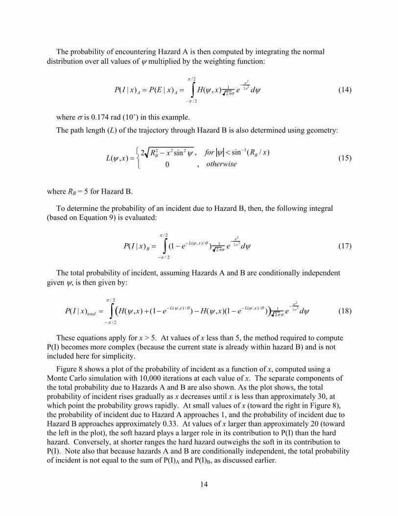
The probability of encountering Hazard A is then computed by integrating the normal distribution over all values of ψ multiplied by the weighting function:

P(I | x)A = P(E | x)A = H(ψ , x) 12πσ e

− ψ2

2σ2 dψ−π / 2

π / 2

∫ (14)

where σ is 0.174 rad (10˚) in this example.

The path length (L) of the trajectory through Hazard B is also determined using geometry:

L(ψ ,x) =2 RB

2 − x2 sin2 ψ0

, for ψ < sin−1(RB / x), otherwise

(15)

where RB = 5 for Hazard B.

To determine the probability of an incident due to Hazard B, then, the following integral (based on Equation 9) is evaluated:

P(I | x)B = (1 − e− L(ψ , x ) / θ ) 12πσ e

− ψ2

2σ 2 dψ−π / 2

π / 2

∫ (17)

The total probability of incident, assuming Hazards A and B are conditionally independent given ψ, is then given by:

P(I | x)total = H(ψ ,x) + (1− e− L(ψ ,x ) / θ ) − H(ψ ,x)(1 − e− L(ψ ,x ) /θ )( ) 12π σ e

− ψ2

2σ 2 dψ− π / 2

π / 2

∫ (18)

These equations apply for x > 5. At values of x less than 5, the method required to compute P(I) becomes more complex (because the current state is already within hazard B) and is not included here for simplicity.

Figure 8 shows a plot of the probability of incident as a function of x, computed using a Monte Carlo simulation with 10,000 iterations at each value of x. The separate components of the total probability due to Hazards A and B are also shown. As the plot shows, the total probability of incident rises gradually as x decreases until x is less than approximately 30, at which point the probability grows rapidly. At small values of x (toward the right in Figure 8), the probability of incident due to Hazard A approaches 1, and the probability of incident due to Hazard B approaches approximately 0.33. At values of x larger than approximately 20 (toward the left in the plot), the soft hazard plays a larger role in its contribution to P(I) than the hard hazard. Conversely, at shorter ranges the hard hazard outweighs the soft in its contribution to P(I). Note also that because hazards A and B are conditionally independent, the total probability of incident is not equal to the sum of P(I)A and P(I)B, as discussed earlier.

14

0

0.1

0.2

0.3

0.4

0.5

0.6

0.7

0.8

0.9

1

0102030405060708090100

x

total

Hazard A (hard)

Hazard B (soft)

P(I)

Figure 8: Example Probability of Incident

Example Application to Aviation Weather Hazards Up to this point, the focus has been on describing a method by which the probability of an

incident can be computed, assuming that a model of the process and the hazards can be developed. This section discusses issues relating to how soft hazards can be modeled, using an aviation weather problem as a case study.

The flight of an aircraft can be modeled generically as a process in which the pilot provides control inputs so as to arrive at some destination state. Along the way, hazards may be encountered that are both internal (e.g., engine fire, excessive loads) and external to the aircraft (e.g., other aircraft, terrain, weather). Currently, alerting systems are in place that warn pilots of hard hazard collision threats such as traffic or terrain. Pilots also have weather radar displays that depict precipitation intensity. Due to the soft, complex nature of weather as a hazard, pilots have traditionally had to integrate weather information with other constraints when determining tactical routes. As more complex alerting systems are developed, it may be attractive to incorporate soft weather information in the decision aids, even if only at a fairly rudimentary level. As the simplified example in Figure 8 showed, soft hazards can be a significant factor at the longer time scales, and such consideration may aid flight planning efforts. Additionally, automated conflict resolution commands to pilots or air traffic controllers may be improved by reducing the likelihood that such a resolution command is not acceptable due to weather.

Weather and Aircraft Interaction Data Collection Weather is a complex hazard, and translating weather information into a form that can be used

by an automated system is a challenge that will continue to be addressed by researchers in the future. As a preliminary step in this direction, however, observations of enroute aircraft

15

proximity to weather were performed to develop a simplified, prototype model of weather as a soft hazard.

Courtesy of the MIT Lincoln Laboratory, archived aircraft track and weather data were obtained for the hours between 2100 GMT on May 19, 1997 to 0900 GMT on May 20, 1997 from the Dallas Fort-Worth enroute sector, which spans 500 nmi from New Mexico across Texas (Rhoda & Pawlak, 1998). The aircraft position information for the enroute airspace above 30,000 ft was updated every six seconds, and the weather precipitation data was updated every five minutes. A total of 1095 aircraft were included in the track data, and the weather data included the location, altitude, and intensity (categorized into six levels) of a line-storm passage. The minimum distance between each aircraft and each level of precipitation was recorded every six seconds in the data file. This enabled the calculation of both the overall minimum distances to weather and also the accumulated durations in each level of weather for each aircraft.

Because the pilots had access to on-board weather radar and also received reports of weather conditions by radio, the aircraft generally avoided the most severe regions of weather. The potential to translate this rerouting behavior into a form that could be incorporated into an automated decision aid was the motivation for this study.

Observed Weather Penetration Of the 1095 aircraft, 353 (32%) penetrated level 2 weather or higher. Because the focus is on

behavior of aircraft that penetrated weather, only the data for the 353 penetrating aircraft are considered here. Figure 9 shows a cumulative distribution of the maximum amount of time that these 353 aircraft spent in levels 2 to 5. The solid lines show the observed duration values; the dashed lines show a model fit that is discussed in more detail below. Duration was defined as the accumulated time spent within a given level or a level of higher intensity. Time in level 2, for example, also includes time spent in levels 3 or higher, and thus serves as a metric of the total time spent within a region of precipitation.

16

0

0.1

0.2

0.3

0.4

0.5

0.6

0.7

0.8

0.9

1

0 50 100 150 200

Duration (sec)

Cum

ulat

ive

Prob

abili

ty

Level 2

Level 3Level 4

Level 5

Figure 9: Cumulative Duration by Precipitation Level

(Solid lines: observed values, Dashed lines: model fit)

Focusing on the solid lines, 90% of the aircraft, for example, spent less than approximately 190 sec inside level 2, and 90% of the aircraft spent less than approximately 25 seconds in level 4. Additionally, the values of the cumulative distribution for a duration of zero indicate the proportion of the 353 aircraft that did not enter each level of weather. For example, approximately 27% of the aircraft that entered level 2 weather did not enter weather of level 3.

The observed penetration times need to be corrected to take into account the fact that the area covered by each level of precipitation varied. Level 5 weather, for example, covered only 9% of the area covered by level 2, and so shorter penetration times would be expected based solely on geometry. Modeling the weather as circular regions and assuming no deviation effects, the expected number of aircraft that would enter each level of weather would be proportional to the radius of each weather cell (or equivalently, the square-root of the area). Furthermore, the expected duration in each level, using this model, would be proportional to the area itself. Table 1 summarizes these relationships. The overall area covered by each level of precipitation is shown, relative to the area covered by level 2. Also shown are the expected and observed fractions of aircraft that entered each level, and the overall expected and observed average duration in each level.

17

Table 1: Expected and Observed Penetration Behavior (Fractions Relative to Level 2)

Precipitation Level

Area fraction

Expected to enter

Observed to enter

Expected duration

Observed duration

2 (reference) 1.00 1.00 1.00 1.00 1.00

3 0.48 0.69 0.73 0.48 0.43

4 0.23 0.48 0.40 0.23 0.14

5 0.09 0.30 0.10 0.09 0.02

6 0.03 0.17 0.00 0.03 0.00

As can be seen in Table 1, increasingly fewer aircraft entered levels 4-6 than would be expected based on the simplified geometrical model of weather. Also, the average duration spent in levels 3 and above was lower than would be predicted by the model. Because on average the durations would have been significantly larger had no route modifications been made, the penetration times in Figure 9 can be used as estimates of the upper limit of time that was acceptable to the pilots to spend in each level of weather.

Hazard Modeling In the approach taken here, each level of precipitation is modeled as a separate, conditionally-

independent hazard. Thus, the total probability of an incident is integrated over the soft hazards encountered along a trajectory, each weighed by some severity factor. When the probability of an incident along an expected trajectory exceeds some threshold, that trajectory is deemed to be unacceptable. It is assumed that aircraft position, trajectory, weather extent, and weather severity information are known accurately. The principal uncertainty then lies in the subjective assessment by each pilot of whether an incident would occur in a certain area of precipitation.

Because none of the aircraft penetrated level 6 weather, level 6 can be adequately modeled as a hard hazard.

Levels 2 through 5, however, had some degree of softness since aircraft did penetrate them. A simplifying assumption is that pilots penetrated the weather only as far as they considered to be acceptable. Because radio transcripts or pilot reports were not available to the authors, it is not known whether any of the penetration events resulted in significant problems for the flight crews or posed other safety threats. The assumption at this stage is that all penetration events were acceptable to the pilots who flew them. With this assumption, another way of interpreting Figure 9 is that the cumulative distribution shows the probability that a pilot would not accept a routing of a given duration. Thus, 90% of the pilots, for example, would not accept a trajectory that remained inside level 4 for more than 25 sec. Similarly, since no aircraft were observed flying more than 150 sec through level 4 precipitation, a trajectory that involves more than 150 sec of flight through level 4 would not be acceptable to any pilot. This assumption is reasonable given the fact that the pilots, on average, originally had significantly longer trajectories through

18

each level of precipitation, but deviated to reduce that exposure according to the cumulative plot in Figure 9.

Using this approach, hazard severities for levels 2-5 were chosen such that the resulting probability of incident for a given length of exposure was similar to the observed cumulative distribution in Figure 9. The result is that the computed probability of incident along a particular trajectory approximates the percentage of pilots that would not accept that trajectory. Thus, a decision threshold can be set based on a desired acceptance percentile. For example, assume that a decision threshold is set at a value of P(I | E) of 0.95. Then, alerts will be generated for 95th percentile weather; that is, weather for which 95% of pilots would agree is hazardous. A more risk-averse approach would be to lower this threshold, but then there may be a significant number of pilots who feel the system is overly conservative.

A reasonable model that fits the observed data is one in which the severity density function fL(l) is of the form shown in Figure 10. For each precipitation level, there is some discrete ‘cost’ or probability of incident that applies any time that type of weather is entered (modeled as an impulse of probability c at zero duration). In addition, there is an exposure-time dependent component that is integrated over the path of the weather, modeled as an exponential distribution with mean time to an incident, θ.

The resultant value for the probability of an incident along a route of length L through precipitation is then given by a modified form of equation (8):

P(I | E) = c + (1 − c)(1 − e− L /θ ) (19)

f (l)L

Duration, l (sec)

c

θ

Duration, l (sec)

c

P(I | E)

Probability Density Function Cumulative Distribution

Figure 10: Model of Weather Severity

A preliminary match to the cumulative distribution in Figure 9 was performed, resulting in the values for c and θ shown in Table 2 for the different levels of precipitation. The curves of P(I) that these parameters produce are shown as the dashed lines in Figure 9.

19

Table 2: Modeled Probability Density Function Parameters

Precipitation Level c θ (sec)

2 0.00 78

3 0.27 40

4 0.60 20

5 0.90 10

6 1.00 —

Using these parameters, an arbitrary weather situation can be analyzed to determine the probability of incident, which is translated directly into the likelihood that a pilot would not accept the given route. Using the methodology developed in the previous section, solutions can be computed for routes that extend over several hazards of varying severity, including hard traffic or terrain threats. Additionally, current state, future trajectory, and hazard extent uncertainties could be included.

Due to the complex nature of weather as a soft hazard, the specific model of weather presented here is rudimentary and is intended only as an illustration of the type of analysis that could be pursued. Future research efforts will focus on further developing this methodology and on analyzing aircraft-weather interactions in more detail, with the goal of enabling the development of decision aids that integrate hard and soft hazard information in a manner that is acceptable to the operators.

Conclusion This paper presents a generalized model that enables incorporating hard and soft hazards into

a single automated decision regarding the acceptability of a particular state trajectory. The model may be used with more than one hazard, of more than one type, in a given problem. Uncertainties in state measurements, dynamics, hazard extent, and severity are included, as is consideration of the fact that different operators may have different concepts of what is an acceptable or unacceptable risk. This potential difference in the definition of what is acceptable is a key issue that needs to be resolved when developing decision aiding systems to monitor soft, subjective threats. In many cases, it is necessary to obtain data during the operation of the system in order to better understand operator preferences and decision-making behavior. This operational data can then be inserted into the design process of future decision aids.

Using an aviation weather case study, information gained from observations of pilot behavior in the presence of weather was used to develop a preliminary model of weather as a soft hazard. This information could then be used in automation to aid operators in monitoring or replanning routes, but additional research is required in this area.

Although an aviation case study was used here, the concepts developed in this paper can be extended to non-aerospace applications in which subjective operational data is inserted into the

20

design process to improve automated decision-making. Examples include process control in which a soft operating envelope may be exceeded, with the result that component failure rates may be increased. Whether an operator would agree to such an envelope exceedance could be determined and used with other dynamic information to develop a decision-aid. Another example could be the use of accident or incident statistics to better understand the nature of soft hazards so as to improve decision logic or alerting thresholds.

Acknowledgments This research was supported by the NASA Ames Research Center under Grant NAG-2-1111

and Contract NAS-2-98012. The authors are appreciative of the support provided by MIT Lincoln Laboratory in providing and analyzing the weather and traffic data, with specific thanks to James Evans, Dale Rhoda, Margo Pawlak, and Beth Bouchard.

References Davis, T., Krzeczowski, K., & C. Bergh (1994), “The Final Approach Spacing Tool”, 13th IFAC

Symposium on Automatic Control in Aerospace, Palo Alto, CA, September. Krozel, J., Weidner, T. & G. Hunter (1997), “Terminal Area Guidance Incorporating Heavy

Weather”, AIAA Guidance, Navigation, and Control Conference, August. Kuchar, J. K. (1996), “Methodology for Alerting-System Performance Evaluation”, AIAA

Journal of Guidance, Control, and Dynamics, Vol. 19, No. 2, March-April. Kuchar, J. K., and B. D. Carpenter (1997), “Airborne Collision Alerting Logic for Closely-

Spaced Parallel Approach”, Air Traffic Control Quarterly, Vol. 5, No. 2. Paielli, R. A. and Erzberger, H. (1997), “Conflict Probability Estimation for Free Flight”, AIAA

Journal of Guidance, Control, and Dynamics. Vol. 20. No. 3. pp. 588-596. Pritchett, A. (1996), “Pilot Non-Conformance to Alerting System Commands During Closely

Spaced Parallel Approaches”, PhD Thesis, Department of Aeronautics and Astronautics, Massachusetts Institute of Technology, Cambridge, MA, December.

Rhoda, D. & M. Pawlak (1998), “The Thunderstorm Penetration / Deviation Decision in the Terminal Area” MIT Lincoln Laboratory Technical Report, Lexington, MA.

Slattery, R., & S. Green (1994), “Conflict-Free Trajectory Planning for Air Traffic Control Automation”, NASA TM-108790, Moffett Field, CA, January.

Wangermann, J. P. & R. F. Stengel (1996), “Optimization and Coordination of Multi-Agent Systems Using Principled Negotiation”, AIAA-96-3853, AIAA Guidance, Navigation, and Control Conference, San Diego, CA, July 29-31.

Yang, L. C., and J. K. Kuchar (1997), “Prototype Conflict Alerting Logic for Free Flight”, AIAA Journal of Guidance, Control, and Dynamics, Vol. 20, No. 4, July-August.

21