Day 5 Limited Dependent Variable Models (Brief) Binary ...cameron.econ.ucdavis.edu/bgpe2011/bgpev2_ldv.pdf · Day 5 Limited Dependent Variable Models (Brief) Binary, multinomial,

Day 5Limited Dependent Variable Models (Brief)

Binary, multinomial, censored, treatment e¤ects

c A. Colin CameronUniv. of Calif. - Davis

Frontiers in EconometricsBavarian Graduate Program in Economics

.Based on A. Colin Cameron and Pravin K. Trivedi (2005),

Microeconometrics: Methods and Applications (MMA), C.U.P.A. Colin Cameron and Pravin K. Trivedi (2009, 2010),Microeconometrics using Stata (MUS), Stata Press.

March 21-25, 2011

c A. Colin Cameron Univ. of Calif. - Davis (Frontiers in Econometrics Bavarian Graduate Program in Economics . Based on A. Colin Cameron and Pravin K. Trivedi (2005), Microeconometrics: Methods and Applications (MMA), C.U.P. A. Colin Cameron and Pravin K. Trivedi (2009, 2010), Microeconometrics using Stata (MUS), Stata Press.)Lectures in Microeconometrics: Brief LDV March 21-25, 2011 1 / 53

1. Introduction

1. Introduction

Abbreviated handout: assumes previous exposure to nonlinear models.

Binary outcomesI y takes only one of two values, say 0 or 1.I model Pr[y = 1jx]I logit and probit are standard

Multinomial outcomesI y takes only m possible outcomes.I model Pr[y = j jx] for j = 1, ...,mI many models including multinomial logit.

Censored and truncated models (e.g. Tobit) and selection modelsI Considerably more di¢ cult conceptually.I Sample is not re�ective of the population (selection on y)I Standard methods rely on strong distributional assumptions.

Treatment evaluation


1. Introduction

Outline

1 Introduction2 Logit and Probit Models3 Multinomial Models4 Censored and truncated data (Tobit)5 Sample selection models6 Treatment Evaluation


2. Logit and Probit models De�nition

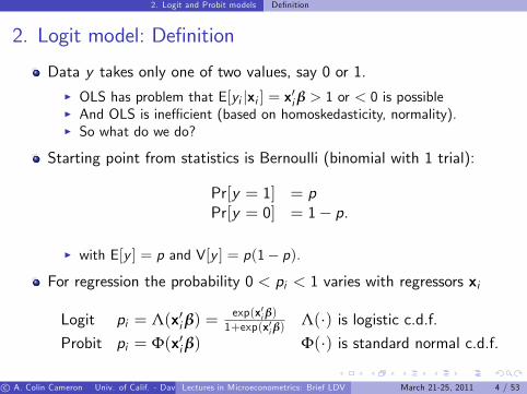
2. Logit model: De�nition

Data y takes only one of two values, say 0 or 1.I OLS has problem that E[yi jxi ] = x0i β > 1 or < 0 is possibleI And OLS is ine¢ cient (based on homoskedasticity, normality).I So what do we do?

Starting point from statistics is Bernoulli (binomial with 1 trial):

Pr[y = 1] = pPr[y = 0] = 1� p.

I with E[y ] = p and V[y ] = p(1� p).

For regression the probability 0 < pi < 1 varies with regressors xi

Logit pi = Λ(x0iβ) =exp(x0i β)1+exp(x0i β)

Λ(�) is logistic c.d.f.Probit pi = Φ(x0iβ) Φ(�) is standard normal c.d.f.


2. Logit and Probit models Example

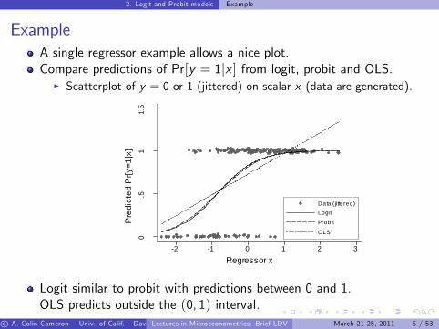
ExampleA single regressor example allows a nice plot.Compare predictions of Pr[y = 1jx ] from logit, probit and OLS.

I Scatterplot of y = 0 or 1 (jittered) on scalar x (data are generated).

0.5

11.

5

Pre

dict

ed P

r[y=1

|x]

-2 -1 0 1 2 3

Regressor x

D ata ( jittered)Logit

Probit

OLS

Logit similar to probit with predictions between 0 and 1.OLS predicts outside the (0, 1) interval.


2. Logit and Probit models Logit and Probit MLE

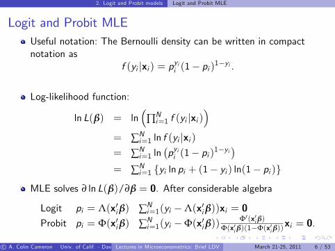
Logit and Probit MLEUseful notation: The Bernoulli density can be written in compactnotation as

f (yi jxi ) = pyii (1� pi )1�yi .

Log-likelihood function:

ln L(β) = ln�

∏Ni=1 f (yi jxi )

�= ∑N

i=1 ln f (yi jxi )= ∑N

i=1 ln�pyii (1� pi )1�yi

�= ∑N

i=1 fyi ln pi + (1� yi ) ln(1� pi )g

MLE solves ∂ ln L(β)/∂β = 0. After considerable algebra

Logit pi = Λ(x0iβ) ∑Ni=1(yi �Λ(x0iβ))xi = 0

Probit pi = Φ(x0iβ) ∑Ni=1(yi �Φ(x0iβ))

Φ0(x0i β)Φ(x0i β)(1�Φ(x0i β))

xi = 0.


2. Logit and Probit models Logit and Probit MLE

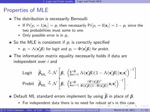
Properties of MLEThe distribution is necessarily Bernoulli

I If Pr[yi = 1jxi ] = pi then necessarily Pr[yi = 0jxi ] = 1� pi since thetwo probabilities must some to one.

I Only possible error is in pi .

So the MLE is consistent if pi is correctly speci�edI pi = Λ(x0i β) for logit and pi = Φ(x0i β) for probit.

The information matrix equality necessarily holds if data areindependent over i and

Logit bβML a� N�

β,�

∑Ni=1 Λ(x0iβ)(1�Λ(x0iβ))xix

0i

��1�Probit bβML a� N

�β,�

∑Ni=1

(Φ0(x0i β)2

Φ(x0i β)(1�Φ(x0i β))xix0i

��1�.

Default ML standard errors implement by using bβ in place of β.

I For independent data there is no need for robust se�s in this case.


2. Logit and Probit models Data example: Private health insurance

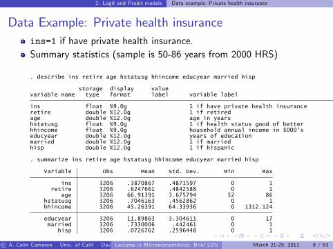
Data Example: Private health insuranceins=1 if have private health insurance.Summary statistics (sample is 50-86 years from 2000 HRS)

hisp 3206 .0726762 .2596448 0 1married 3206 .7330006 .442461 0 1

educyear 3206 11.89863 3.304611 0 17

hhincome 3206 45.26391 64.33936 0 1312.124hstatusg 3206 .7046163 .4562862 0 1

age 3206 66.91391 3.675794 52 86retire 3206 .6247661 .4842588 0 1

ins 3206 .3870867 .4871597 0 1

Variable Obs Mean Std. Dev. Min Max

. summarize ins retire age hstatusg hhincome educyear married hisp

hisp double %12.0g 1 if hispanicmarried double %12.0g 1 if marriededucyear double %12.0g years of educationhhincome float %9.0g household annual income in $000'shstatusg float %9.0g 1 if health status good of betterage double %12.0g age in yearsretire double %12.0g 1 if retiredins float %9.0g 1 if have private health insurance

variable name type format label variable labelstorage display value

. describe ins retire age hstatusg hhincome educyear married hisp


2. Logit and Probit models Data example: Private health insurance

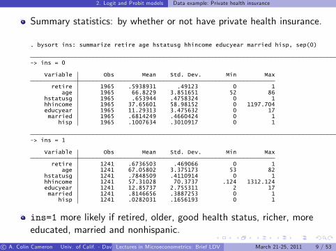
Summary statistics: by whether or not have private health insurance.

hisp 1241 .0282031 .1656193 0 1married 1241 .8146656 .3887253 0 1

educyear 1241 12.85737 2.755311 2 17hhincome 1241 57.31028 70.3737 .124 1312.124hstatusg 1241 .7848509 .4110914 0 1

age 1241 67.05802 3.375173 53 82retire 1241 .6736503 .469066 0 1


-> ins = 1

hisp 1965 .1007634 .3010917 0 1married 1965 .6814249 .4660424 0 1

educyear 1965 11.29313 3.475632 0 17hhincome 1965 37.65601 58.98152 0 1197.704hstatusg 1965 .653944 .4758324 0 1

age 1965 66.8229 3.851651 52 86retire 1965 .5938931 .49123 0 1


-> ins = 0

. bysort ins: summarize retire age hstatusg hhincome educyear married hisp, sep(0)

ins=1 more likely if retired, older, good health status, richer, moreeducated, married and nonhispanic.


2. Logit and Probit models Logit data example

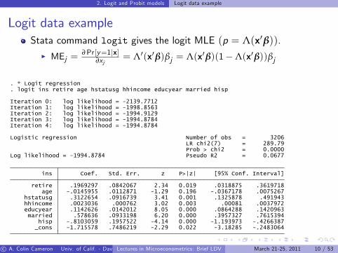
Logit data exampleStata command logit gives the logit MLE (p = Λ(x0β)).

I MEj =∂Pr[y=1jx]

∂xj= Λ0(x0β)βj = Λ(x0β)(1�Λ(x0β))βj

_cons -1.715578 .7486219 -2.29 0.022 -3.18285 -.2483064hisp -.8103059 .1957522 -4.14 0.000 -1.193973 -.4266387

married .578636 .0933198 6.20 0.000 .3957327 .7615394educyear .1142626 .0142012 8.05 0.000 .0864288 .1420963hhincome .0023036 .000762 3.02 0.003 .00081 .0037972hstatusg .3122654 .0916739 3.41 0.001 .1325878 .491943

age -.0145955 .0112871 -1.29 0.196 -.0367178 .0075267retire .1969297 .0842067 2.34 0.019 .0318875 .3619718

ins Coef. Std. Err. z P>|z| [95% Conf. Interval]

Log likelihood = -1994.8784 Pseudo R2 = 0.0677Prob > chi2 = 0.0000LR chi2(7) = 289.79

Logistic regression Number of obs = 3206

Iteration 4: log likelihood = -1994.8784Iteration 3: log likelihood = -1994.8784Iteration 2: log likelihood = -1994.9129Iteration 1: log likelihood = -1998.8563Iteration 0: log likelihood = -2139.7712

. logit ins retire age hstatusg hhincome educyear married hisp

. * Logit regression

All except perhaps hstatusg have the expected sign.c A. Colin Cameron Univ. of Calif. - Davis (Frontiers in Econometrics Bavarian Graduate Program in Economics . Based on A. Colin Cameron and Pravin K. Trivedi (2005), Microeconometrics: Methods and Applications (MMA), C.U.P. A. Colin Cameron and Pravin K. Trivedi (2009, 2010), Microeconometrics using Stata (MUS), Stata Press.)Lectures in Microeconometrics: Brief LDV March 21-25, 2011 10 / 53

2. Logit and Probit models Logit data example

Average marginal e¤ectAMEj = 1

N ∑Ni=1

∂Pr[yi=1jxi ]∂xj

= 1N ∑N

i=1 Λ(x0β)(1�Λ(x0β))βjCompute AME after logit using Stata 11 margins, dydx(*) orStata 10 add-on command margeff.

hisp -.175951 .0421962 -4.17 0.000 -.258654 -.0932481married .1256459 .0198205 6.34 0.000 .0867985 .1644933

educyear .0248111 .0029705 8.35 0.000 .0189891 .0306332hhincome .0005002 .0001646 3.04 0.002 .0001777 .0008228hstatusg .0678058 .0197778 3.43 0.001 .0290419 .1065696

age -.0031693 .0024486 -1.29 0.196 -.0079686 .00163retire .0427616 .018228 2.35 0.019 .0070354 .0784878

dy/dx Std. Err. z P>|z| [95% Conf. Interval]Delta-method

dy/dx w.r.t. : retire age hstatusg hhincome educyear married hispExpression : Pr(ins), predict()

Model VCE : OIMAverage marginal effects Number of obs = 3206

Warning: cannot perform check for estimable functions.. margins, dydx(*)

Marginal e¤ects: 0.043, -0.003, 0.067, 0.0005, 0.025, 0.126, -0.176vs.Coe¢ cients: 0.197, -0.015, 0.312, 0.0023, 0.114, 0.579, -0.810.

I Marginal e¤ect here is about one-�fth the size of the coe¢ cient.

I Could use �nite di¤erences for binary regressors.c A. Colin Cameron Univ. of Calif. - Davis (Frontiers in Econometrics Bavarian Graduate Program in Economics . Based on A. Colin Cameron and Pravin K. Trivedi (2005), Microeconometrics: Methods and Applications (MMA), C.U.P. A. Colin Cameron and Pravin K. Trivedi (2009, 2010), Microeconometrics using Stata (MUS), Stata Press.)Lectures in Microeconometrics: Brief LDV March 21-25, 2011 11 / 53

2. Logit and Probit models Probit data example

Probit data example

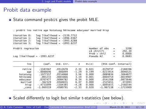
Stata command probit gives the probit MLE.

_cons -1.069319 .4580791 -2.33 0.020 -1.967138 -.1715009hisp -.4731099 .1104385 -4.28 0.000 -.6895655 -.2566544


age -.0088696 .006899 -1.29 0.199 -.0223914 .0046521retire .1183567 .0512678 2.31 0.021 .0178737 .2188396

ins Coef. Std. Err. z P>|z| [95% Conf. Interval]


Probit regression Number of obs = 3206

Iteration 3: log likelihood = -1993.6237Iteration 2: log likelihood = -1993.6288Iteration 1: log likelihood = -1996.0367Iteration 0: log likelihood = -2139.7712

. probit ins retire age hstatusg hhincome educyear married hisp

Scaled di¤erently to logit but similar t-statistics (see below).


2. Logit and Probit models OLS data example

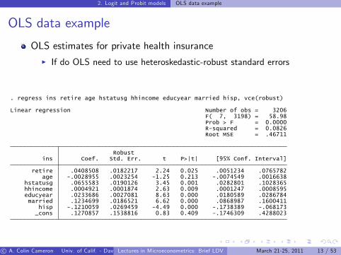
OLS data example

OLS estimates for private health insuranceI If do OLS need to use heteroskedastic-robust standard errors

_cons .1270857 .1538816 0.83 0.409 -.1746309 .4288023hisp -.1210059 .0269459 -4.49 0.000 -.1738389 -.068173


age -.0028955 .0023254 -1.25 0.213 -.0074549 .0016638retire .0408508 .0182217 2.24 0.025 .0051234 .0765782

ins Coef. Std. Err. t P>|t| [95% Conf. Interval]Robust

Root MSE = .46711R-squared = 0.0826Prob > F = 0.0000F( 7, 3198) = 58.98

Linear regression Number of obs = 3206

. regress ins retire age hstatusg hhincome educyear married hisp, vce(robust)


2. Logit and Probit models Comparison of models

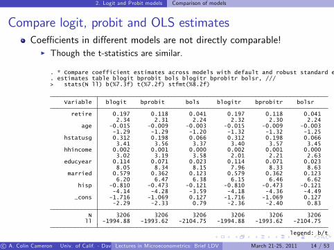
Compare logit, probit and OLS estimatesCoe¢ cients in di¤erent models are not directly comparable!

I Though the t-statistics are similar.

legend: b/t

ll -1994.88 -1993.62 -2104.75 -1994.88 -1993.62 -2104.75N 3206 3206 3206 3206 3206 3206

-2.29 -2.33 0.79 -2.36 -2.40 0.83_cons -1.716 -1.069 0.127 -1.716 -1.069 0.127

-4.14 -4.28 -3.59 -4.18 -4.36 -4.49hisp -0.810 -0.473 -0.121 -0.810 -0.473 -0.121

6.20 6.47 6.38 6.15 6.46 6.62married 0.579 0.362 0.123 0.579 0.362 0.123

8.05 8.34 8.15 7.96 8.33 8.63educyear 0.114 0.071 0.023 0.114 0.071 0.023

3.02 3.19 3.58 2.01 2.21 2.63hhincome 0.002 0.001 0.000 0.002 0.001 0.000

3.41 3.56 3.37 3.40 3.57 3.45hstatusg 0.312 0.198 0.066 0.312 0.198 0.066

-1.29 -1.29 -1.20 -1.32 -1.32 -1.25age -0.015 -0.009 -0.003 -0.015 -0.009 -0.003

2.34 2.31 2.24 2.32 2.30 2.24retire 0.197 0.118 0.041 0.197 0.118 0.041

Variable blogit bprobit bols blogitr bprobitr bolsr

> stats(N ll) b(%7.3f) t(%7.2f) stfmt(%8.2f). estimates table blogit bprobit bols blogitr bprobitr bolsr, ///. * Compare coefficient estimates across models with default and robust standard errors


2. Logit and Probit models Comparison of predicted probabilities

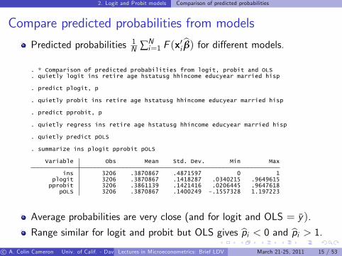
Compare predicted probabilities from models

Predicted probabilities 1N ∑N

i=1 F (x0i bβ) for di¤erent models.

pOLS 3206 .3870867 .1400249 -.1557328 1.197223pprobit 3206 .3861139 .1421416 .0206445 .9647618plogit 3206 .3870867 .1418287 .0340215 .9649615

ins 3206 .3870867 .4871597 0 1


. summarize ins plogit pprobit pOLS

. quietly predict pOLS

. quietly regress ins retire age hstatusg hhincome educyear married hisp

. predict pprobit, p

. quietly probit ins retire age hstatusg hhincome educyear married hisp

. predict plogit, p

. quietly logit ins retire age hstatusg hhincome educyear married hisp

. * Comparison of predicted probabilities from logit, probit and OLS

Average probabilities are very close (and for logit and OLS = y).

Range similar for logit and probit but OLS gives bpi < 0 and bpi > 1.c A. Colin Cameron Univ. of Calif. - Davis (Frontiers in Econometrics Bavarian Graduate Program in Economics . Based on A. Colin Cameron and Pravin K. Trivedi (2005), Microeconometrics: Methods and Applications (MMA), C.U.P. A. Colin Cameron and Pravin K. Trivedi (2009, 2010), Microeconometrics using Stata (MUS), Stata Press.)Lectures in Microeconometrics: Brief LDV March 21-25, 2011 15 / 53

2. Logit and Probit models Marginal e¤ects: Approximations

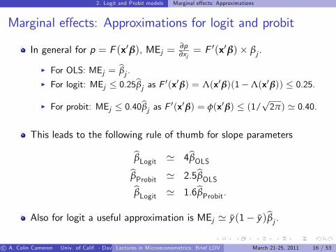
Marginal e¤ects: Approximations for logit and probit

In general for p = F (x0β), MEj = ∂p∂xj= F 0(x0β)� βj .

I For OLS: MEj = bβj .I For logit: MEj � 0.25bβj as F 0(x0β) = Λ(x0β)(1�Λ(x0β)) � 0.25.

I For probit: MEj � 0.40bβj as F 0(x0β) = φ(x0β) � (1/p2π) ' 0.40.

This leads to the following rule of thumb for slope parameters

bβLogit ' 4bβOLSbβProbit ' 2.5bβOLSbβLogit ' 1.6bβProbit.Also for logit a useful approximation is MEj ' y(1� y)bβj .


2. Logit and Probit models Which model?

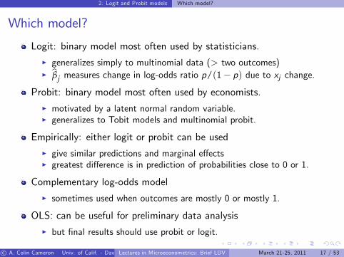
Which model?

Logit: binary model most often used by statisticians.I generalizes simply to multinomial data (> two outcomes)I bβj measures change in log-odds ratio p/(1� p) due to xj change.

Probit: binary model most often used by economists.I motivated by a latent normal random variable.I generalizes to Tobit models and multinomial probit.

Empirically: either logit or probit can be usedI give similar predictions and marginal e¤ectsI greatest di¤erence is in prediction of probabilities close to 0 or 1.

Complementary log-odds modelI sometimes used when outcomes are mostly 0 or mostly 1.

OLS: can be useful for preliminary data analysisI but �nal results should use probit or logit.


3. Multinomial models De�nition

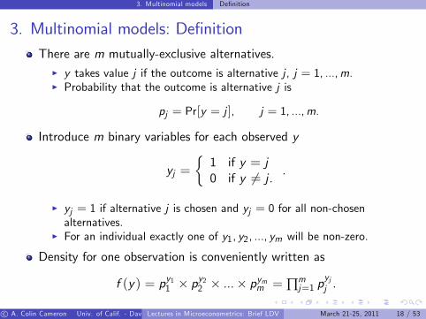
3. Multinomial models: De�nitionThere are m mutually-exclusive alternatives.

I y takes value j if the outcome is alternative j , j = 1, ...,m.I Probability that the outcome is alternative j is

pj = Pr[y = j ], j = 1, ...,m.

Introduce m binary variables for each observed y

yj =�1 if y = j0 if y 6= j . .

I yj = 1 if alternative j is chosen and yj = 0 for all non-chosenalternatives.

I For an individual exactly one of y1, y2, ..., ym will be non-zero.

Density for one observation is conveniently written as

f (y) = py11 � py22 � ...� pymm = ∏m

j=1 pyjj .


3. Multinomial models Regression model

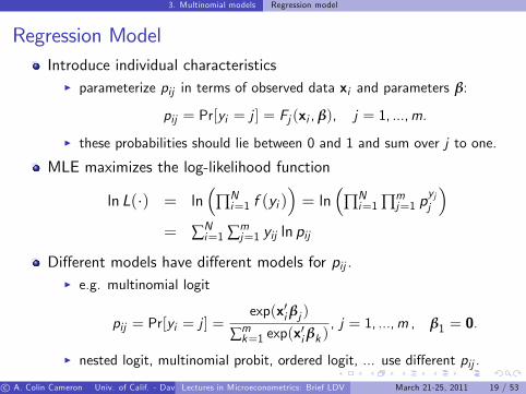
Regression ModelIntroduce individual characteristics

I parameterize pij in terms of observed data xi and parameters β:

pij = Pr[yi = j ] = Fj (xi , β), j = 1, ...,m.

I these probabilities should lie between 0 and 1 and sum over j to one.

MLE maximizes the log-likelihood function

ln L(�) = ln�

∏Ni=1 f (yi )

�= ln

�∏Ni=1 ∏m

j=1 pyjj

�= ∑N

i=1 ∑mj=1 yij ln pij

Di¤erent models have di¤erent models for pij .I e.g. multinomial logit

pij = Pr[yi = j ] =exp(x0i βj )

∑mk=1 exp(x0i βk )

, j = 1, ...,m , β1 = 0.

I nested logit, multinomial probit, ordered logit, ... use di¤erent pij .


3. Multinomial models Data Example: Fishing site

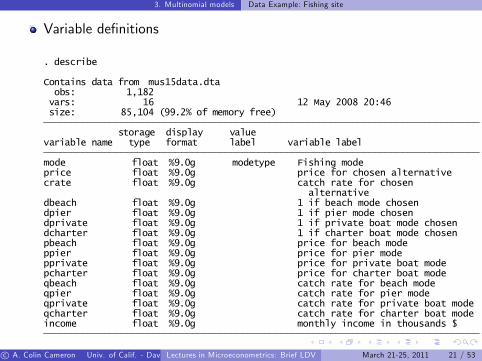
Data example: Fishing site

Multinomial variable y has outcome one ofI y = 1 if �sh from beachI y = 2 if �sh from pierI y = 3 if �sh from private boatI y = 4 if �sh from charter boat

Regressors areI price: varies by alternative and individualI catch rate: varies by alternative and individualI income: varies by individual but not alternative



Variable de�nitions

income float %9.0g monthly income in thousands $qcharter float %9.0g catch rate for charter boat modeqprivate float %9.0g catch rate for private boat modeqpier float %9.0g catch rate for pier modeqbeach float %9.0g catch rate for beach modepcharter float %9.0g price for charter boat modepprivate float %9.0g price for private boat modeppier float %9.0g price for pier modepbeach float %9.0g price for beach modedcharter float %9.0g 1 if charter boat mode chosendprivate float %9.0g 1 if private boat mode chosendpier float %9.0g 1 if pier mode chosendbeach float %9.0g 1 if beach mode chosen

alternativecrate float %9.0g catch rate for chosenprice float %9.0g price for chosen alternativemode float %9.0g modetype Fishing mode

variable name type format label variable label storage display value

size: 85,104 (99.2% of memory free) vars: 16 12 May 2008 20:46 obs: 1,182Contains data from mus15data.dta

. describe



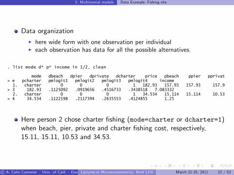
Data organizationI here wide form with one observation per individualI each observation has data for all the possible alternatives.

> 4 34.534 .1122198 .2117394 .2635553 .4124855 1.25 2. charter 0 0 0 1 34.534 15.114 15.114 10.53> 3 182.93 .1125092 .0919656 .4516733 .3438518 7.083332 1. charter 0 0 0 1 182.93 157.93 157.93 157.9> e pcharter pmlogit1 pmlogit2 pmlogit3 pmlogit4 income

mode dbeach dpier dprivate dcharter price pbeach ppier pprivat

. list mode d* p* income in 1/2, clean

Here person 2 chose charter �shing (mode=charter or dcharter=1)when beach, pier, private and charter �shing cost, respectively,15.11, 15.11, 10.53 and 34.53.



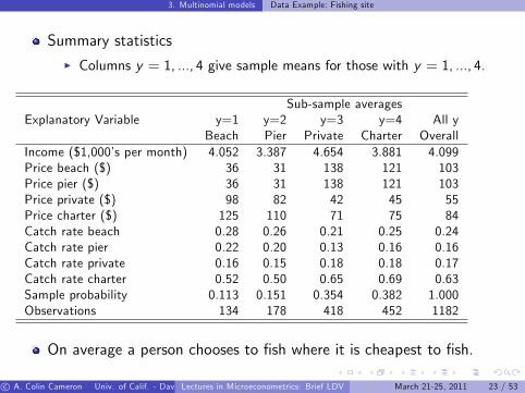
Summary statisticsI Columns y = 1, ..., 4 give sample means for those with y = 1, ..., 4.

Sub-sample averagesExplanatory Variable y=1 y=2 y=3 y=4 All y

Beach Pier Private Charter OverallIncome ($1,000�s per month) 4.052 3.387 4.654 3.881 4.099Price beach ($) 36 31 138 121 103Price pier ($) 36 31 138 121 103Price private ($) 98 82 42 45 55Price charter ($) 125 110 71 75 84Catch rate beach 0.28 0.26 0.21 0.25 0.24Catch rate pier 0.22 0.20 0.13 0.16 0.16Catch rate private 0.16 0.15 0.18 0.18 0.17Catch rate charter 0.52 0.50 0.65 0.69 0.63Sample probability 0.113 0.151 0.354 0.382 1.000Observations 134 178 418 452 1182

On average a person chooses to �sh where it is cheapest to �sh.


3. Multinomial models Multinomial logit data example

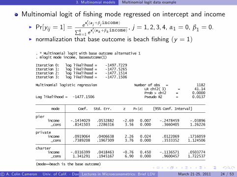
Multinomial logit of �shing mode regressed on intercept and income

I Pr[yij = 1] =ex0i (αj+βjincome)

∑4k=1 ex0i (αk+βkincome)

, j = 1, 2, 3, 4, α1 = 0, β1 = 0.

I normalization that base outcome is beach �shing (y = 1)

(mode==beach is the base outcome)

_cons 1.341291 .1945167 6.90 0.000 .9600457 1.722537 income -.0316399 .0418463 -0.76 0.450 -.1136571 .0503774charter

_cons .7389208 .1967309 3.76 0.000 .3533352 1.124506 income .0919064 .0406638 2.26 0.024 .0122069 .1716059private

_cons .8141503 .2286316 3.56 0.000 .3660405 1.26226 income -.1434029 .0532882 -2.69 0.007 -.2478459 -.03896pier

mode Coef. Std. Err. z P>|z| [95% Conf. Interval]

Log likelihood = -1477.1506 Pseudo R2 = 0.0137Prob > chi2 = 0.0000LR chi2( 3) = 41.14

Multinomial logistic regression Number of obs = 1182

Iteration 3: log likelihood = -1477.1506Iteration 2: log likelihood = -1477.1514Iteration 1: log likelihood = -1477.5265Iteration 0: log likelihood = -1497.7229

. mlogit mode income, baseoutcome(1)

. * Multinomial logit with base outcome alternative 1



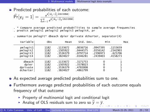
Predicted probabilities of each outcome:bPr[yij = 1] = ex0i (bαj+bβjincome)

∑4k=1 e

x0i (bαk+bβkincome)

dcharter 1182 .3824027 .4861799 0 1dprivate 1182 .3536379 .4783008 0 1

dpier 1182 .1505922 .3578023 0 1 dbeach 1182 .1133672 .3171753 0 1

pmlogit4 1182 .3824027 .0346281 .2439403 .4158273pmlogit3 1182 .3536379 .0797714 .2396973 .625706pmlogit2 1182 .1505922 .0444575 .0356142 .2342903

pmlogit1 1182 .1133672 .0036716 .0947395 .1153659


. summarize pmlogit* dbeach dpier dprivate dcharter, separator(4)

. predict pmlogit1 pmlogit2 pmlogit3 pmlogit4, pr

. * Compare average predicted probabilities to sample average frequencies

As expected average predicted probabilities sum to one.

Furthermore average predicted probabilities of each outcome equalsfrequency of that outcome

I Property of multinomial logit and conditional logitI Analog of OLS residuals sum to zero so by = y .



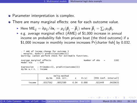
Parameter interpretation is complex.

There are many marginal e¤ects: one for each outcome value.I Here MEij = ∂pij/∂xi = pij (βj � βi ) where βi = ∑l pilβl .I e.g. average marginal e¤ect (AME) of $1,000 increase in annualincome on probability �sh from private boat (the third outcome) if a$1,000 increase in monthly income increases Pr[charter �sh] by 0.032.

income .0317562 .0052589 6.04 0.000 .021449 .0420633

dy/dx Std. Err. z P>|z| [95% Conf. Interval]Delta-method

dy/dx w.r.t. : incomeExpression : Pr(mode==3), predict(outcome(3))

Model VCE : OIMAverage marginal effects Number of obs = 1182

Warning: cannot perform check for estimable functions.. margins, dydx(*) predict(outcome(3)). * AME of income change for outcome 3


3. Multinomial models Further detail

Further details

bβ is consistently asymptotically normal by the usual asymptotictheory if the d.g.p. is correctly speci�ed.

I The distribution is necessarily multinomial.I So key is correct speci�cation of pij = Fj (xi , β).I And no need to use vce(robust) option if independent data.

Distinguish between two di¤erent types of regressors.I Alternative-speci�c or case-speci�c or alternative-invariant regressorsdo not vary across alternatives.

F e.g. income (in our example), gender.

I Alternative-varying regressors may vary across alternatives.

F e.g. price.

I Multinomial logit: all regressors are individual-speci�c.I Conditional logit: same as multinomial logit regressors are alternativevarying.


3. Multinomial models Unordered models

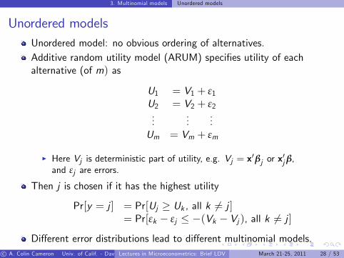
Unordered modelsUnordered model: no obvious ordering of alternatives.Additive random utility model (ARUM) speci�es utility of eachalternative (of m) as

U1 = V1 + ε1U2 = V2 + ε2...

......

Um = Vm + εm

I Here Vj is deterministic part of utility, e.g. Vj = x0βj or x0jβ,

and εj are errors.

Then j is chosen if it has the highest utility

Pr[y = j ] = Pr[Uj � Uk , all k 6= j ]= Pr[εk � εj � �(Vk � Vj ), all k 6= j ]

Di¤erent error distributions lead to di¤erent multinomial models.c A. Colin Cameron Univ. of Calif. - Davis (Frontiers in Econometrics Bavarian Graduate Program in Economics . Based on A. Colin Cameron and Pravin K. Trivedi (2005), Microeconometrics: Methods and Applications (MMA), C.U.P. A. Colin Cameron and Pravin K. Trivedi (2009, 2010), Microeconometrics using Stata (MUS), Stata Press.)Lectures in Microeconometrics: Brief LDV March 21-25, 2011 28 / 53

3. Multinomial models Examples of Unordered models

Examples of unordered Models

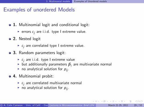
1. Multinomial logit and conditional logit:I errors εj are i.i.d. type I extreme value.

2. Nested logitI εj are correlated type I extreme value.

3. Random parameters logit:I εj are i.i.d. type I extreme valueI but additionally parameters βi are multivariate normalI no analytical solution for pij .

4. Multinomial probit:I εj are correlated multivariate normalI no analytical solution for pij .


3. Multinomial models Examples of Unordered models

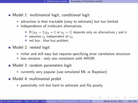
Model 1: multinomial logit, conditional logitI attraction is that tractable (easy to estimate) but too limitedI independence of irrelevant alternatives

F Pr[yik = 1jyik = 1 or yij = 1] depends only on alternatives j and kF assumes εij independent of εikF red bus - blue bus problem.

Model 2: nested logitI richer and still easy but requires specifying error correlation structureI two versions - only one consistent with ARUM

Model 3: random parameters logitI currently very popular (use simulated ML or Bayesian)

Model 4: multinomial probitI potentially rich but hard to estimate and �ts poorly.


3. Multinomial models Ordered models

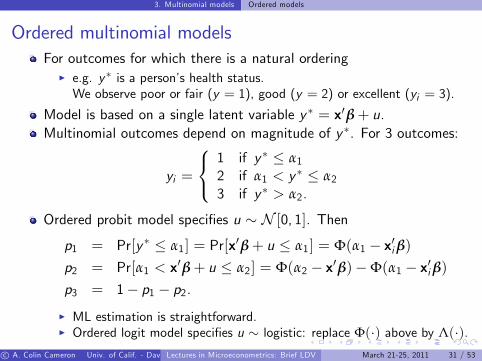
Ordered multinomial modelsFor outcomes for which there is a natural ordering

I e.g. y� is a person�s health status.We observe poor or fair (y = 1), good (y = 2) or excellent (yi = 3).

Model is based on a single latent variable y � = x0β+ u.Multinomial outcomes depend on magnitude of y �. For 3 outcomes:

yi =

8<:1 if y � � α12 if α1 < y � � α23 if y � > α2.

Ordered probit model speci�es u � N [0, 1]. Thenp1 = Pr[y � � α1] = Pr[x0β+ u � α1] = Φ(α1 � x0iβ)p2 = Pr[α1 < x0β+ u � α2] = Φ(α2 � x0β)�Φ(α1 � x0iβ)p3 = 1� p1 � p2.I ML estimation is straightforward.I Ordered logit model speci�es u � logistic: replace Φ(�) above by Λ(�).


3. Multinomial models Stata commands

Stata commands

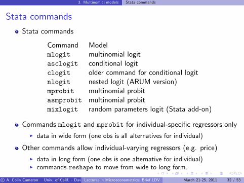
Stata commands

Command Modelmlogit multinomial logitasclogit conditional logitclogit older command for conditional logitnlogit nested logit (ARUM version)mprobit multinomial probitasmprobit multinomial probitmixlogit random parameters logit (Stata add-on)

Commands mlogit and mprobit for individual-speci�c regressors onlyI data in wide form (one obs is all alternatives for individual)

Other commands allow individual-varying regressors (e.g. price)I data in long form (one obs is one alternative for individual)I commands reshape to move from wide to long form.


4. Censored and Truncated data Tobit

4. Censored data: Tobit

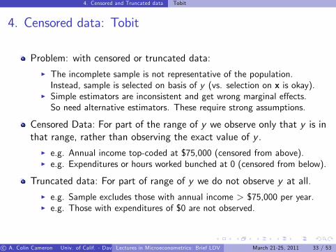
Problem: with censored or truncated data:I The incomplete sample is not representative of the population.Instead, sample is selected on basis of y (vs. selection on x is okay).

I Simple estimators are inconsistent and get wrong marginal e¤ects.So need alternative estimators. These require strong assumptions.

Censored Data: For part of the range of y we observe only that y is inthat range, rather than observing the exact value of y .

I e.g. Annual income top-coded at $75,000 (censored from above).I e.g. Expenditures or hours worked bunched at 0 (censored from below).

Truncated data: For part of range of y we do not observe y at all.I e.g. Sample excludes those with annual income > $75,000 per year.I e.g. Those with expenditures of $0 are not observed.


4. Censored and Truncated data De�nition

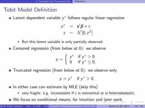
Tobit Model De�nitionLatent dependent variable y � follows regular linear regression

y � = x0β+ ε

ε � N [0, σ2]

I But this latent variable is only partially observed.

Censored regression (from below at 0): we observe

y =�y � if y � > 00 if y � � 0.

Truncated regression (from below at 0): we observe only

y = y � if y � > 0.

In either case can estimate by MLE (skip this)I very fragile: e.g. inconsistent if ε is nonnormal or is heteroskedastic.

We focus on conditional means, for intuition and later work.c A. Colin Cameron Univ. of Calif. - Davis (Frontiers in Econometrics Bavarian Graduate Program in Economics . Based on A. Colin Cameron and Pravin K. Trivedi (2005), Microeconometrics: Methods and Applications (MMA), C.U.P. A. Colin Cameron and Pravin K. Trivedi (2009, 2010), Microeconometrics using Stata (MUS), Stata Press.)Lectures in Microeconometrics: Brief LDV March 21-25, 2011 34 / 53

4. Censored and Truncated data Tobit example with simulated data

Tobit example with Simulated Data

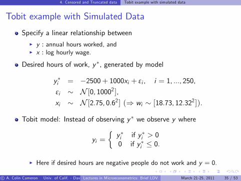
Specify a linear relationship betweenI y : annual hours worked, andI x : log hourly wage.

Desired hours of work, y �, generated by model

y �i = �2500+ 1000xi + εi , i = 1, ..., 250,

εi � N [0, 10002],xi � N [2.75, 0.62] () wi � [18.73, 12.322]).

Tobit model: Instead of observing y � we observe y where

yi =�y �i if y �i > 00 if y �i � 0.

I Here if desired hours are negative people do not work and y = 0.


4. Censored and Truncated data Tobit example with simulated data

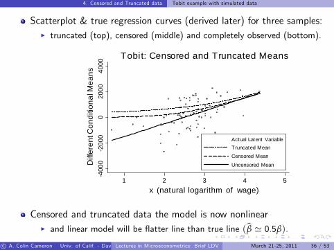
Scatterplot & true regression curves (derived later) for three samples:I truncated (top), censored (middle) and completely observed (bottom).

-400

0-2

000

020

0040

00D

iffer

ent C

ondi

tiona

l Mea

ns

1 2 3 4 5x (natural logarithm of wage)

Actual Latent VariableTruncated MeanCensored Mean

Uncensored Mean

Tobit: Censored and Truncated Means

Censored and truncated data the model is now nonlinearI and linear model will be �atter line than true line (bβ ' 0.5β).


4. Censored and Truncated data Truncated mean in Tobit model

Truncated Mean in Tobit model

Truncated mean: We observe y only when y > 0.

The truncated conditional mean (suppressing conditioning on x) is

E[y jy > 0]= E [x0β+ εjx0β+ ε > 0] as y = x0β+ ε= x0β+ E [εjε > �x0β] as x and ε independent

= x0β+ σEh

εσ j

εσ >

�x0βσ

itransform to ε/σ � N [0, 1]

= x0β+ σλ�x0βσ

�using next slide: key result for N [0, 1].

I where λ(z) = φ(z)/Φ(z) is called the inverse Mills ratio.

The regression function is not just x0β (and is nonlinear).I OLS of y on x is inconsistent for βI Need NLS or MLE for consistent estimates.


4. Censored and Truncated data Truncated mean for standard normal

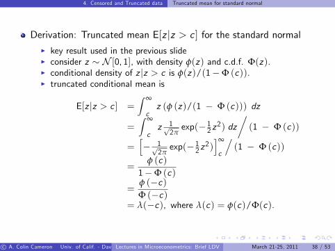
Derivation: Truncated mean E[z jz > c ] for the standard normalI key result used in the previous slideI consider z � N [0, 1], with density φ(z) and c.d.f. Φ(z).I conditional density of z jz > c is φ(z)/(1�Φ (c)).I truncated conditional mean is

E[z jz > c ] =Z ∞

cz (φ (z)/(1 � Φ (c))) dz

=Z ∞

cz 1p

2πexp(� 12 z2) dz

�(1 � Φ (c))

=h� 1p

2πexp(� 12 z2)

i∞

c

.(1 � Φ (c))

=φ (c)

1�Φ (c)

=φ (�c)Φ (�c)

= λ(�c), where λ(c) = φ(c)/Φ(c).


4. Censored and Truncated data Censored mean

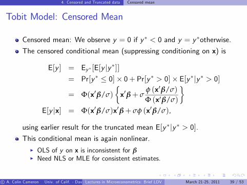
Tobit Model: Censored Mean

Censored mean: We observe y = 0 if y � < 0 and y = y �otherwise.

The censored conditional mean (suppressing conditioning on x) is

E[y ] = Ey � [E[y jy �]]= Pr[y � � 0]� 0+ Pr[y � > 0]� E[y �jy � > 0]

= Φ(x0β/σ)

�x0β+ σ

φ (x0β/σ)

Φ (x0β/σ)

�E[y jx] = Φ(x0β/σ)x0β+ σφ (x0β/σ),

using earlier result for the truncated mean E[y �jy � > 0].This conditional mean is again nonlinear.

I OLS of y on x is inconsistent for βI Need NLS or MLE for consistent estimates.


4. Censored and Truncated data Data Example

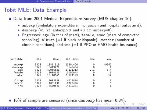
Tobit MLE: Data ExampleData from 2001 Medical Expenditure Survey (MUS chapter 16).

I ambexp (ambulatory expenditure = physician and hospital outpatient).I dambexp (=1 if ambexp>0 and =0 if ambexp=0).I Regressors: age (in tens of years), female, educ (years of completedschooling), blhisp (=1 if black or hispanic) , totchr (number ofchronic conditions), and ins (=1 if PPO or HMO health insurance).

ins 3328 .3650841 .4815261 0 1totchr 3328 .4831731 .7720426 0 5blhisp 3328 .3085938 .4619824 0 1

educ 3328 13.40565 2.574199 0 17female 3328 .5084135 .5000043 0 1

age 3328 4.056881 1.121212 2.1 6.4dambexp 3328 .8419471 .3648454 0 1ambexp 3328 1386.519 2530.406 0 49960


16% of sample are censored (since dambexp has mean 0.84).


4. Censored and Truncated data Data Example

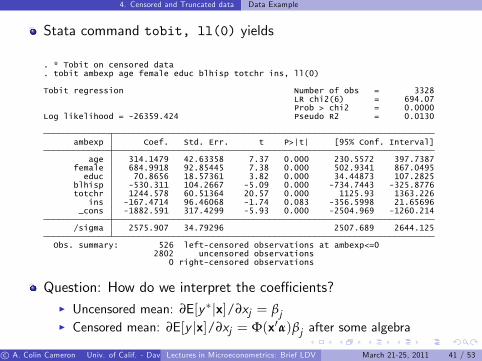
Stata command tobit, ll(0) yields

0 right-censored observations2802 uncensored observations

Obs. summary: 526 left-censored observations at ambexp<=0

/sigma 2575.907 34.79296 2507.689 2644.125

_cons -1882.591 317.4299 -5.93 0.000 -2504.969 -1260.214ins -167.4714 96.46068 -1.74 0.083 -356.5998 21.65696

totchr 1244.578 60.51364 20.57 0.000 1125.93 1363.226blhisp -530.311 104.2667 -5.09 0.000 -734.7443 -325.8776

educ 70.8656 18.57361 3.82 0.000 34.44873 107.2825female 684.9918 92.85445 7.38 0.000 502.9341 867.0495

age 314.1479 42.63358 7.37 0.000 230.5572 397.7387

ambexp Coef. Std. Err. t P>|t| [95% Conf. Interval]


Tobit regression Number of obs = 3328

. tobit ambexp age female educ blhisp totchr ins, ll(0)

. * Tobit on censored data

Question: How do we interpret the coe¢ cients?I Uncensored mean: ∂E[y�jx]/∂xj = βjI Censored mean: ∂E[y jx]/∂xj = Φ(x0α)βj after some algebra


4. Censored and Truncated data Limitations

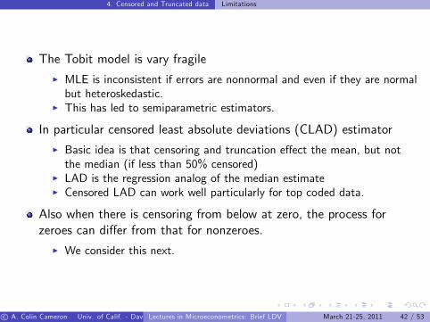
The Tobit model is vary fragileI MLE is inconsistent if errors are nonnormal and even if they are normalbut heteroskedastic.

I This has led to semiparametric estimators.

In particular censored least absolute deviations (CLAD) estimatorI Basic idea is that censoring and truncation e¤ect the mean, but notthe median (if less than 50% censored)

I LAD is the regression analog of the median estimateI Censored LAD can work well particularly for top coded data.

Also when there is censoring from below at zero, the process forzeroes can di¤er from that for nonzeroes.

I We consider this next.


5. Sample Selection Models Overview

5. Sample Selection Model: Overview

There are many generalizations of standard Tobit, often involvingsample selection or self-selection.

We consider the most common, Heckman�s sample selection modelI Also called type 2 Tobit, Tobit with stochastic threshold, Tobit withprobit selection.

I For censoring below this is often more realistic than standard Tobit,as it allows di¤erent equations for participation and the outcome.


5. Sample Selection Models De�nition

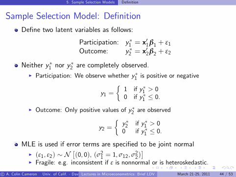
Sample Selection Model: De�nitionDe�ne two latent variables as follows:

Participation: y �1 = x01β1 + ε1

Outcome: y �2 = x02β2 + ε2

Neither y �1 nor y�2 are completely observed.

I Participation: We observe whether y�1 is positive or negative

y1 =�1 if y�1 > 00 if y�1 � 0.

I Outcome: Only positive values of y�2 are observed

y2 =�y�2 if y�1 > 00 if y�1 � 0.

MLE is used if error terms are speci�ed to be joint normalI (ε1, ε2) � N

�(0, 0), (σ21 = 1, σ12, σ

22)�

I Fragile: e.g. inconsistent if ε is nonnormal or is heteroskedastic.


5. Sample Selection Models Heckman 2-step estimator

Sample Selection Model: Heckman 2-step estimator

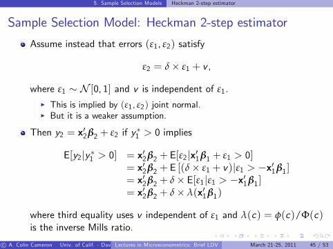
Assume instead that errors (ε1, ε2) satisfy

ε2 = δ� ε1 + v ,

where ε1 � N [0, 1] and v is independent of ε1.I This is implied by (ε1, ε2) joint normal.I But it is a weaker assumption.

Then y2 = x02β2 + ε2 if y �1 > 0 implies

E[y2jy �1 > 0] = x02β2 + E[ε2jx01β1 + ε1 > 0]= x02β2 + E [(δ� ε1 + v)jε1 > �x01β1]= x02β2 + δ� E[ε1jε1 > �x01β1]= x02β2 + δ� λ(x01β1)

where third equality uses v independent of ε1 and λ(c) = φ(c)/Φ(c)is the inverse Mills ratio.



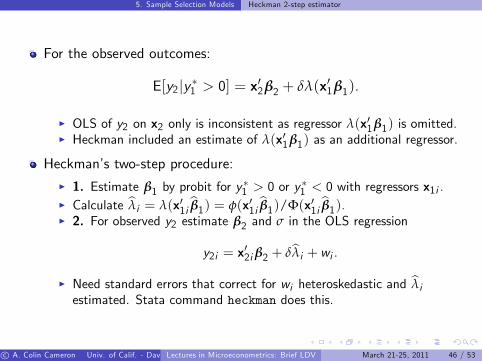
For the observed outcomes:

E[y2jy �1 > 0] = x02β2 + δλ(x01β1).

I OLS of y2 on x2 only is inconsistent as regressor λ(x01β1) is omitted.I Heckman included an estimate of λ(x01β1) as an additional regressor.

Heckman�s two-step procedure:I 1. Estimate β1 by probit for y

�1 > 0 or y

�1 < 0 with regressors x1i .

I Calculate bλi = λ(x01i bβ1) = φ(x01i bβ1)/Φ(x01i bβ1).I 2. For observed y2 estimate β2 and σ in the OLS regression

y2i = x02i β2 + δbλi + wi .I Need standard errors that correct for wi heteroskedastic and bλiestimated. Stata command heckman does this.



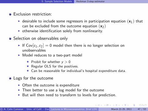
Exclusion restriction:I desirable to include some regressors in participation equation (x1) thatcan be excluded from the outcome equation (x2)

I otherwise identi�cation solely from nonlinearity.

Selection on observables onlyI If Cov[ε1, ε2 ] = 0 model then there is no longer selection onunobservables

I Model reduces to a two-part model

F Probit for whether y > 0F Regular OLS for the positives.F Can be reasonable for individual�s hospital expenditure data.

Logs for the outcomeI Often the outcome is expenditureI Then better to use a log model for the outcomeI But will then need to transform to levels for prediction.



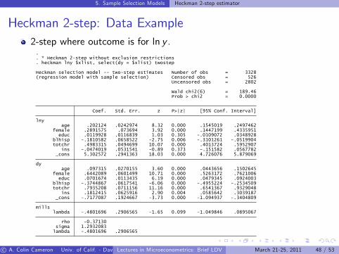
Heckman 2-step: Data Example2-step where outcome is for ln y .

lambda -.4801696 .2906565sigma 1.2932083

rho -0.37130

lambda -.4801696 .2906565 -1.65 0.099 -1.049846 .0895067mills

_cons -.7177087 .1924667 -3.73 0.000 -1.094937 -.3404809ins .1812415 .0625916 2.90 0.004 .0585642 .3039187

totchr .7935208 .0711156 11.16 0.000 .6541367 .9329048blhisp -.3744867 .0617541 -6.06 0.000 -.4955224 -.2534509

educ .0701674 .0113435 6.19 0.000 .0479345 .0924003female .6442089 .0601499 10.71 0.000 .5263172 .7621006

age .097315 .0270155 3.60 0.000 .0443656 .1502645dy

_cons 5.302572 .2941363 18.03 0.000 4.726076 5.879069ins -.0474019 .0531541 -0.89 0.373 -.151582 .0567782

totchr .4983315 .0494699 10.07 0.000 .4013724 .5952907blhisp -.1810582 .0658522 -2.75 0.006 -.3101261 -.0519904

educ .0119928 .0116839 1.03 0.305 -.0109072 .0348928female .2891575 .073694 3.92 0.000 .1447199 .4335951

age .202124 .0242974 8.32 0.000 .1545019 .2497462lny

Coef. Std. Err. z P>|z| [95% Conf. Interval]

Prob > chi2 = 0.0000Wald chi2(6) = 189.46

Uncensored obs = 2802(regression model with sample selection) Censored obs = 526Heckman selection model -- two-step estimates Number of obs = 3328

. heckman lny $xlist, select(dy = $xlist) twostep

. * Heckman 2-step without exclusion restrictions

.


5. Sample Selection Models Stata commands

Stata commands

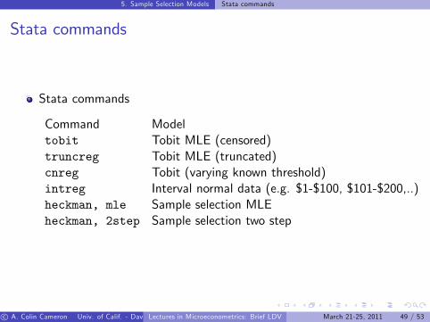
Stata commands

Command Modeltobit Tobit MLE (censored)truncreg Tobit MLE (truncated)cnreg Tobit (varying known threshold)intreg Interval normal data (e.g. $1-$100, $101-$200,..)heckman, mle Sample selection MLEheckman, 2step Sample selection two step


6. Treatment e¤ects models Treatment e¤ects problem

6. Treatment e¤ects models

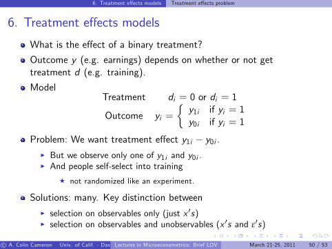
What is the e¤ect of a binary treatment?

Outcome y (e.g. earnings) depends on whether or not gettreatment d (e.g. training).

ModelTreatment di = 0 or di = 1

Outcome yi =�y1i if yi = 1y0i if yi = 1

Problem: We want treatment e¤ect y1i � y0i .I But we observe only one of y1i and y0i .I And people self-select into training

F not randomized like an experiment.

Solutions: many. Key distinction betweenI selection on observables only (just x 0s)I selection on observables and unobservables (x 0s and ε0s)


6. Treatment e¤ects models Selection on Observables Only

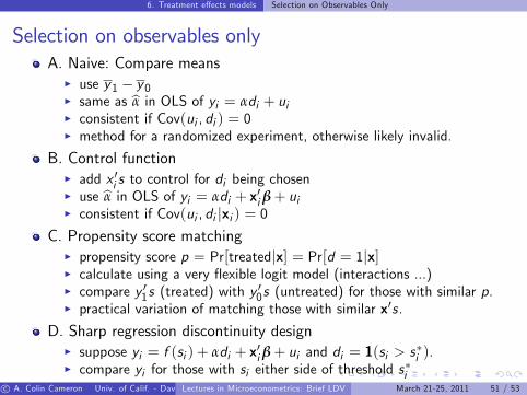
Selection on observables onlyA. Naive: Compare means

I use y1 � y0I same as bα in OLS of yi = αdi + uiI consistent if Cov(ui , di ) = 0I method for a randomized experiment, otherwise likely invalid.

B. Control functionI add x 0i s to control for di being chosenI use bα in OLS of yi = αdi + x0i β+ uiI consistent if Cov(ui , di jxi ) = 0

C. Propensity score matchingI propensity score p = Pr[treatedjx] = Pr[d = 1jx]I calculate using a very �exible logit model (interactions ...)I compare y 01s (treated) with y

00s (untreated) for those with similar p.

I practical variation of matching those with similar x0s.

D. Sharp regression discontinuity designI suppose yi = f (si ) + αdi + x0i β+ ui and di = 1(si > s

�i ).

I compare yi for those with si either side of threshold s�ic A. Colin Cameron Univ. of Calif. - Davis (Frontiers in Econometrics Bavarian Graduate Program in Economics . Based on A. Colin Cameron and Pravin K. Trivedi (2005), Microeconometrics: Methods and Applications (MMA), C.U.P. A. Colin Cameron and Pravin K. Trivedi (2009, 2010), Microeconometrics using Stata (MUS), Stata Press.)Lectures in Microeconometrics: Brief LDV March 21-25, 2011 51 / 53

6. Treatment e¤ects models Selection on Observables and Unobservables

Selection on observables and unobservables

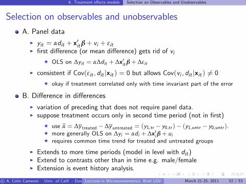
A. Panel dataI yit = αdit + x0itβ+ vi + εitI �rst di¤erence (or mean di¤erence) gets rid of vi

F OLS on ∆yit = α∆dit + ∆x0itβ+ ∆εit

I consistent if Cov(εit , dit jxit ) = 0 but allows Cov(vi , dit jxit ) 6= 0F okay if treatment correlated only with time invariant part of the error

B. Di¤erence in di¤erencesI variation of preceding that does not require panel data.I suppose treatment occurs only in second time period (not in �rst)

F use bα = ∆y treated � ∆y untreated = (y1,tr � y0,tr)� (y1,untr � y0,untr).F more generally OLS on ∆yi = αdi + ∆x0i β+ uiF requires common time trend for treated and untreated groups

I Extends to more time periods (model in level with dit )I Extend to contrasts other than in time e.g. male/femaleI Extension is event history analysis.


6. Treatment e¤ects models Selection on Observables and Unobservables

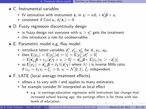
C. Instrumental variablesI IV estimation with instrument zi in yi = αdi + x0i β+ uiI consistent if Cov(ui , di jxi ) = 0

D. Fuzzy regression discontinuity designI in fuzzy design not everyone with si > s�i gets the treatment.I this introduces a role for unobservables.

E. Parametric model e,g, Roy model:I introduce latent variables d�i , y

�1i , y

�0i for di , y1i , y0i .

I then E[y1i ] = E[y�1i jdi = 1] = E[y�1i jd�i > 0]= E[x01i β+ ε1i jz0iγ+ vi > 0] = x01i β+ E[ε1i jvi > �z0iγ]

I so E[y1i ] = x01i β+ δ1λ(z0iγ) where λ(�) is inverse Mills ratioif ε1i = δ1vi + ξ i > 0, vi � N [0, 1], ξ i independent.

F. LATE (local average treatment e¤ects)I allows α to vary with i and applies to many estimators.I for example consider IV interpreted as local e¤ect

F e.g. in earnings-education regression with instrument law change thatincreased school leaving age, the earnings e¤ect is for those with lowlevels of education.


Documents

Day 5 Limited Dependent Variable Models (Brief) Binary ...cameron.econ.ucdavis.edu/bgpe2011/bgpev2_ldv.pdf · Day 5 Limited Dependent Variable Models (Brief) Binary, multinomial,