Embed Size (px)
Citation preview

DC Mach ines
p c machines are characterized by their versatility. By means of various com- binations of shunt-, series-, and separately-excited field windings they can be designed to display a wide variety of volt-ampere or speed-torque character-
istics for both dynamic and steady-state operation. Because of the ease with which they can be controlled, systems of dc machines have been frequently used in appli- cations requiring a wide range of motor speeds or precise control of motor output. In recent years, solid-state ac drive system technology has developed sufficiently that these systems are replacing dc machines in applications previously associated almost exclusively with dc machines. However, the versatility of dc machines in combination with the relative simplicity of their drive systems will insure their continued use in a wide variety of applications.
7.1 I N T R O D U C T I O N The essential features of a dc machine are shown schematically in Fig. 7.1. The stator has salient poles and is excited by one or more field coils. The air-gap flux distribution created by the field windings is symmetric about the center line of the field poles. This axis is called the field axis or direct axis.
As discussed in Section 4.6.2, the ac voltage generated in each rotating arma- ture coil is converted to dc in the external armature terminals by means of a rotating commutator and stationary brushes to which the armature leads are connected. The commutator-brush combination forms a mechanical rectifier, resulting in a dc arma- ture voltage as well as an armature-mmf wave which is fixed in space. Commutator action is discussed in detail in Section 7.2.
The brushes are located so that commutation occurs when the coil sides are in the neutral zone, midway between the field poles. The axis of the armature-mmf wave then is 90 electrical degrees from the axis of the field poles, i.e., in the quadrature axis. In the schematic representation of Fig. 7.1 a, the brushes are shown in the quadrature axis
357

358 CHAPTER 7 DC Machines
Onnclrnhlro
Direct
Brushes axis Field
ield oil
Armature
coils
(a) (b)
Figure 7.1 Schematic representations of a dc machine.
because this is the position of the coils to which they are connected. The armature-mmf wave then is along the brush axis, as shown. (The geometric position of the brushes in an actual machine is approximately 90 electrical degrees from their position in the schematic diagram because of the shape of the end connections to the commutator. For example, see Fig. 7.7.) For simplicity, the circuit representation usually will be drawn as in Fig. 7.1 b.
Although the magnetic torque and the speed voltage appearing at the brushes are somewhat dependent on the spatial waveform of the flux distribution, for convenience we continue to assume a sinusoidal flux-density wave in the air gap as was done in Chapter 4. The torque can then be found from the magnetic field viewpoint of Section 4.7.2.
The electromagnetic torque Tmech can be expressed in terms of the interaction of the direct-axis air-gap flux per pole ~d and the space-fundamental component Fal of the armature-mmf wave, in a form similar to Eq. 4.81. With the brushes in the quadrature axis, the angle between these fields is 90 electrical degrees, and its sine equals unity. Substitution in Eq. 4.81 then gives
7r ( p ° l e s ) 2 Tmech -- ~- 2 ~d Fal (7.1)
in which the minus sign has been dropped because the positive direction of the torque can be determined from physical reasoning. The peak value of the sawtooth armature- mmf wave is given by Eq. 4.9, and its space fundamental Fal is 8/zr 2 times its peak. Substitution in Eq. 7.1 then gives
Tmech'-(p°lesCa) ~dia-Kadpdia2rrm (7.2)

7.1 Introduction 359
Brush voltage e a
X ~ ) Rectified coilvoltages
t
Figure 7 .2 Rectified coil voltages and resultant voltage between brushes in a dc machine.
where
and
ia -- current in external armature circuit
Ca "-" total number of conductors in armature winding
m - number of parallel paths through winding
poles Ca ga = (7.3)
27rm
is a constant determined by the design of the winding. The rectified voltage generated in the armature has already been found in Sec-
tion 4.6.2 for an elementary single-coil armature, and its waveform is shown in Fig. 4.33. The effect of distributing the winding in several slots is shown in Fig. 7.2, in which each of the rectified sine waves is the voltage generated in one of the coils, with commutation taking place at the moment when the coil sides are in the neutral zone.
The generated voltage as observed from the brushes is the sum of the rectified voltages of all the coils in series between brushes and is shown by the rippling line labeled ea in Fig. 7.2. With a dozen or so commutator segments per pole, the ripple becomes very small and the average generated voltage observed from the brushes equals the sum of the average values of the rectified coil voltages. From Eq. 4.53 the rectified voltage ea between brushes, known also as the speed voltage, is
(p° les Ca) ~dC0m -- Ka~dC0 m (7.4) ea -- 2zrm
where Ka is the winding constant defined in Eq. 7.3. The rectified voltage of a dis- tributed winding has the same average value as that of a concentrated coil. The difference is that the ripple is greatly reduced.
From Eqs. 7.2 and 7.4, with all variables expressed in SI units,
eaia-- TmechO)m (7.5)
Noting that the product of torque and mechanical speed is the mechanical power, this equation simply says that the instantaneous electric power associated with the speed voltage equals the instantaneous mechanical power associated with the magnetic
360 CHAPTER 7 DC Machines
~d
Air-gap -,~--'
ZNfif
ea0
Air-gap - ~ / / f
Speed -- Ogmo
ENfif
(a) (b)
ea0
// Air-gap - - - - ~ / Y
Speed = O)m0
r
tf
(c)
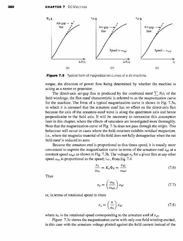
Figure 7.3 Typical form of magnetization curves of a dc machine.
torque, the direction of power flow being determined by whether the machine is acting as a motor or generator.
The direct-axis air-gap flux is produced by the combined mmf ~ Nfif of the field windings; the flux-mmf characteristic is referred to as the magnetization curve for the machine. The form of a typical magnetization curve is shown in Fig. 7.3a, in which it is assumed that the armature mmf has no effect on the direct-axis flux because the axis of the armature-mmf wave is along the quadrature axis and hence perpendicular to the field axis. It will be necessary to reexamine this assumption later in this chapter, where the effects of saturation are investigated more thoroughly. Note that the magnetization curve of Fig. 7.3a does not pass through the origin. This behaviour will occur in cases where the field structure exhibits residual magnetism, i.e., where the magnetic material of the field does not fully demagnetize when the net field mmf is reduced to zero.
Because the armature emf is proportional to flux times speed, it is usually more convenient to express the magnetization curve in terms of the armature emf ea0 at a constant speed Wm0 as shown in Fig. 7.3b. The voltage ea for a given flux at any other speed O-)m is proportional to the speed; i.e., from Eq. 7.4
ea ea0 - - K a ~ d - - (7.6)
O)m Ogm0
Thus
e a - - - - ea0 (7.7) O)m0
or, in terms of rotational speed in r/min
(n) ea - - - - eao
n o (7.8)
where no is the rotational speed corresponding to the armature emf of ea0.
Figure 7.3c shows the magnetization curve with only one field winding excited, in this case with the armature voltage plotted against the field current instead of the

7.1 Introduction 361
field ampere-turns. This curve can easily be obtained by test methods; since the field current can be measured directly, no knowledge of any design details is required.
Over a fairly wide range of excitation the reluctance of the electrical steel in the machine is negligible compared with that of the air gap. In this region the flux is linearly proportional to the total mmf of the field windings, the constant of propor- tionality being the direct-axis permeance/gd; thus
fYPd --- ~')d Z Nfif (7.9)
The dashed straight line through the origin coinciding with the straight portion of the magnetization curves in Fig. 7.3 is called the air-gap line. This nomenclature refers to the fact that this linear magnetizing characteristic would be found if the reluctance of the magnetic material portion of the flux path remained negligible compared to that of the air gap, independent of the degree of magnetic saturation of the motor steel.
The outstanding advantages of dc machines arise from the wide variety of oper- ating characteristics which can be obtained by selection of the method of excitation of the field windings. Various connection diagrams are shown in Fig. 7.4. The method of excitation profoundly influences both the steady-state characteristics and the dynamic behavior of the machine in control systems.
Consider first dc generators. The connection diagram of a separately-excited generator is given in Fig. 7.4a. The required field current is a very small fraction of the rated armature current; on the order of 1 to 3 percent in the average generator. A small amount of power in the field circuit may control a relatively large amount of power in the armature circuit; i.e., the generator is a power amplifier. Separately- excited generators are often used in feedback control systems when control of the armature voltage over a wide range is required.
The field windings of self-excited generators may be supplied in three different ways. The field may be connected in series with the armature (Fig. 7.4b), resulting in
o
Field Armature
o source
o
(a) (b)
Field Field ~ ~ o rheostat rheostat
field ~ Sf~e~dt Sf~il7 .. O
(c ) (d )
Figure 7.4 Field-circuit connections of dc machines: (a) separate excitation, (b) series, (c) shunt, (d) compound.

3 6 2 C H A P T E R 7 DC Machines
0 100
o 75
~ 50
~b
N 25
t Shunt
S e p a r a t e l ~ ....-- - - = - " - - - - - - - - - - . . . . . . . . .
m •
i
i i
- / I
I I
/ I I I I r
0 25 50 75 100
Load current in percent of rating
Figure 7.5 Volt-ampere characteristics of dc generators.
a series generator. The field may be connected in shunt with the armature (Fig. 7.4c), resulting in a shunt generator, or the field may be in two sections (Fig. 7.4d), one of which is connected in series and the other in shunt with the armature, resulting in a compound generator. With self-excited generators, residual magnetism must be present in the machine iron to get the self-excitation process started. The effects of residual magnetism can be clearly seen in Fig. 7.3, where the flux and voltage are seen to have nonzero values when the field current is zero.
Typical steady-state volt-ampere characteristics of dc generators are shown in Fig. 7.5, constant-speed operation being assumed. The relation between the steady- state generated emf Ea and the armature terminal voltage Va is
Va - E a - taRa (7 .10)
where la is the armature current output and Ra is the armature circuit resistance. In a generator, Ea is larger than Va, and the electromagnetic torque Tmech is a countertorque opposing rotation.
The terminal voltage of a separately-excited generator decreases slightly with an increase in the load current, principally because of the voltage drop in the armature resistance. The field current of a series generator is the same as the load current, so that the air-gap flux and hence the voltage vary widely with load. As a consequence, series generators are not often used. The voltage of shunt generators drops off somewhat with load, but not in a manner that is objectionable for many purposes. Compound generators are normally connected so that the mmf of the series winding aids that of the shunt winding. The advantage is that through the action of the series winding the flux per pole can increase with load, resulting in a voltage output which is nearly constant or which even rises somewhat as load increases. The shunt winding usually contains many turns of relatively small wire. The series winding, wound on the outside, consists of a few turns of comparatively heavy conductor because it must carry the full armature current of the machine. The voltage of both shunt and compound

7.1 Introduction 3 6 3
%-.
o 100
75
~ 5 o -
~ 2 5 -
OUnc 1
Shunt ~ -
_ ~ " ~
% %
%,
0 I I I I 0 25 50 75 100
Load torque in percent of rating
Figure 7.6 Speed-torque characteristics of dc motors.
generators can be controlled over reasonable limits by means of rheostats in the shunt field.
Any of the methods of excitation used for generators can also be used for motors. Typical steady-state dc-motor speed-torque characteristics are shown in Fig. 7.6, in which it is assumed that the motor terminals are supplied from a constant-voltage source. In a motor the relation between the emf Ea generated in the armature and the armature terminal voltage Va is
Va = Ea + IaR. (7.11)
or Va m Ea
Ia - (7.12) Ra
where Ia is now the armature-current input to the machine. The generated emf Ea is now smaller than the terminal voltage Va, the armature current is in the opposite direction to that in a generator, and the electromagnetic torque is in the direction to sustain rotation of the armature.
In shunt- and separately-excited motors, the field flux is nearly constant. Conse- quently, increased torque must be accompanied by a very nearly proportional increase in armature current and hence by a small decrease in counter emf Ea to allow this increased current through the small armature resistance. Since counter emf is deter- mined by flux and speed (Eq. 7.4), the speed must drop slightly. Like the squirrel-cage induction motor, the shunt motor is substantially a constant-speed motor having about 6 percent drop in speed from no load to full load. A typical speed-torque characteris- tic is shown by the solid curve in Fig. 7.6. Starting torque and maximum torque are limited by the armature current that can be successfully commutated.
An outstanding advantage of the shunt motor is ease of speed control. With a rheostat in the shunt-field circuit, the field current and flux per pole can be varied at will, and variation of flux causes the inverse variation of speed to maintain counter

3 6 4 C H A P T E R 7 DC Machines
emf approximately equal to the impressed terminal voltage. A maximum speed range of about 4 or 6 to 1 can be obtained by this method, the limitation again being commutating conditions. By variation of the impressed armature voltage, very wide speed ranges can be obtained.
In the series motor, increase in load is accompanied by increases in the arma- ture current and mmf and the stator field flux (provided the iron is not completely saturated). Because flux increases with load, speed must drop in order to maintain the balance between impressed voltage and counter emf; moreover, the increase in armature current caused by increased torque is smaller than in the shunt motor be- cause of the increased flux. The series motor is therefore a varying-speed motor with a markedly drooping speed-torque characteristic of the type shown in Fig. 7.6. For applications requiting heavy torque overloads, this characteristic is particularly ad- vantageous because the corresponding power overloads are held to more reasonable values by the associated speed drops. Very favorable starting characteristics also result from the increase in flux with increased armature current.
In the compound motor, the series field may be connected either cumulatively, so that its mmf adds to that of the shunt field, or differentially, so that it opposes. The differential connection is rarely used. As shown by the broken-dash curve in Fig. 7.6, a cumulatively-compounded motor has speed-load characteristics intermediate be- tween those of a shunt and a series motor, with the drop of speed with load depending on the relative number of ampere-tums in the shunt and series fields. It does not have the disadvantage of very high light-load speed associated with a series motor, but it retains to a considerable degree the advantages of series excitation.
The application advantages of dc machines lie in the variety of performance characteristics offered by the possibilities of shunt, series, and compound excitation. Some of these characteristics have been touched upon briefly in this section. Still greater possibilities exist if additional sets of brushes are added so that other voltages can be obtained from the commutator. Thus the versatility of dc-machine systems and their adaptability to control, both manual and automatic, are their outstanding features.
7.2 C O M M U T A T O R A C T I O N The dc machine differs in several respects from the ideal model of Section 4.2.2. Although the basic concepts of Section 4.2.2 are still valid, a reexamination of the assumptions and a modification of the model are desirable. The crux of the matter is the effect of the commutator shown in Figs. 4.2 and 4.16.
Figure 7.7 shows diagrammatically the armature winding of Figs. 4.22 and 4.23a with the addition of the commutator, brushes, and connections of the coils to the commutator segments. The commutator is represented by the ring of segments in the center of the figure. The segments are insulated from each other and from the shaft. Two stationary brushes are shown by the black rectangles inside the commutator. Actually the brushes usually contact the outer surface, as shown in Fig. 4.16. The coil sides in the slots are shown in cross section by the small circles with dots and crosses in them, indicating currents toward and away from the reader, respectively, as in Fig. 4.22. The connections of the coils to the commutator segments are shown by
7.2 Commutator Action 365
V1
~!ii!!~i~i!~i!~!iii!iii~iiiiiii!!!i~iiii~iJiiJJ~i!iiiii!~ii~i~i~ii~ii~i~iii~ii~i~i~i~i~iJi~iiJ .... / V ~!~i~i~i~i~i~i!ii!!i~iii!i~}ii!iii!i~ii}i~}~!ii!iii~iiiii!ii~i~i~iii~i~!i!i~i~ii~ ~̧ / i iiji:i Yli}iiiii:'i}i}iiiiiiiii/!i!}!iii}iiiii}i}i}ii}ii i: 10 /
f / iiii!iiiii::i!iiiii;iliiii!!ii!iiiilililiiiiiiiiii ;;ill i!il iiiiiii iiiiiiiiiiii!!!i!iiiiiiiiiii!iiiiiii I
i..i iiiii!i!iiiiiii!ii ii!ii 9,,
NI
i Magnetic axis of armature
12..__ ___.... 1 i
11 ¢--' ~ NN2 / .).
7 "'6 (a)
\ \
Field coil
NI
V1
NI
T / / / \ \
/
i\ IQ® ~'. ~b l l - > - / a ~ X A
(b)
j j /
/ /
FI
IE]
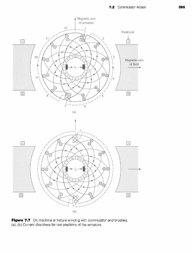
Figure 7.7 Dc machine armature winding with commutator and brushes. (a), (b) Current directions for two positions of the armature.

366 CHAPTER 7 DC Machines
the circular arcs. The end connections at the back of the armature are shown dashed for the two coils in slots 1 and 7, and the connections of these coils to adjacent commutator segments are shown by the heavy arcs. All coils are identical. The back end connections of the other coils have been omitted to avoid complicating the figure, but they can easily be traced by remembering that each coil has one side in the top of a slot and the other side in the bottom of the diametrically-opposite slot.
In Fig. 7.7a the brushes are in contact with commutator segments 1 and 7. Current entering the fight-hand brush divides equally between two parallel paths through the winding. The first path leads to the inner coil side in slot 1 and finally ends at the brush on segment 7. The second path leads to the outer coil side in slot 6 and also finally ends at the brush on segment 7. The current directions in Fig. 7.7a can readily be verified by tracing these two paths. They are the same as in Fig. 4.22. The effect is identical to that of a coil wrapped around the armature with its magnetic axis vertical, and a clockwise magnetic torque is exerted on the armature, tending to align its magnetic field with that of the field winding.
Now suppose the machine is acting as a generator driven in the counterclockwise direction by an applied mechanical torque. Figure 7.7b shows the situation after the armature has rotated through the angle subtended by half a commutator segment. The right-hand brush is now in contact with both segments 1 and 2, and the left-hand brush is in contact with both segments 7 and 8. The coils in slots 1 and 7 are now short-circuited by the brushes. The currents in the other coils are shown by the dots and crosses, and they produce a magnetic field whose axis again is vertical.
After further rotation, the brushes will be in contact with segments 2 and 8, and slots 1 and 7 will have rotated into the positions which were previously occupied by slots 12 and 6 in Fig. 7.7a. The current directions will be similar to those of Fig. 7.7a except that the currents in the coils in slots 1 and 7 will have reversed. The magnetic axis of the armature is still vertical.
During the time when the brushes are simultaneously in contact with two ad- jacent commutator segments, the coils connected to these segments are temporarily removed from the main circuit comprising the armature winding, short-circuited by the brushes, and the currents in them are reversed. Ideally, the current in the coils being commutated should reverse linearly with time, a condition referred to as linear commutation. Serious departure from linear commutation will result in sparking at the brushes. Means for obtaining sparkless commutation are discussed in Section 7.9. With linear commutation the waveform of the current in any coil as a function of time is trapezoidal, as shown in Fig. 7.8.
Commutation , ~ , l
i | Coil current
Figure 7.8 Waveform of current in an armature coil with linear commutation.

7.3 Effect of Armature MMF 367
The winding of Fig. 7.7 is simpler than that used in most dc machines. Ordi- narily more slots and commutator segments would be used, and except in small ma- chines, more than two poles are common. Nevertheless, the simple winding of Fig. 7.7 includes the essential features of more complicated windings.
7.3 EFFECT OF A R M A T U R E MMF Armature mmf has definite effects on both the space distribution of the air-gap flux and the magnitude of the net flux per pole. The effect on flux distribution is important because the limits of successful commutation are directly influenced; the effect on flux magnitude is important because both the generated voltage and the torque per unit of armature current are influenced thereby. These effects and the problems arising from them are described in this section.
It was shown in Section 4.3.2 and Fig. 4.23 that the armature-mmf wave can be closely approximated by a sawtooth, corresponding to the wave produced by a finely-distributed armature winding or current sheet. For a machine with brushes in the neutral position, the idealized mmf wave is again shown by the dashed sawtooth in Fig. 7.9, in which a positive mmf ordinate denotes flux lines leaving the armature surface. Current directions in all windings other than the main field are indicated by black and cross-hatched bands. Because of the salient-pole field structure found in almost all dc machines, the associated space distribution of flux will not be triangular. The distribution of air-gap flux density with only the armature excited is given by the solid curve of Fig. 7.9. As can readily be seen, it is appreciably decreased by the long air path in the interpolar space.
%%%%%
i
I II Field coi
Finely distributed ' Finely distributed I~) conductors (~ conductors
on armature on armature S ' '% S %
Motor s S r o t a ~
S s S Armature-mmf
S ," distribution
% ",, Generator
~ ~ ' ~ ~ a t i o n
Flux-density "" ~ ~ ~ " ' ~ ' ~ % s
' distribution with " , , ' s S % s
only the armature ",, s 'excited
F igu re 7.9 Armature-mmf and flux-density distribution with brushes on neutral and only the armature excited.

368 CHAPTER 7 DC Machines
Field iron
Armature iron
Figure 7.10 Flux with only the armature excited and brushes on neutral.
The axis of the armature mmf is fixed at 90 electrical degrees from the main- field axis by the brush position. The corresponding flux follows the paths shown in Fig. 7.10. The effect of the armature mmf is seen to be that of creating flux crossing the pole faces; thus its path in the pole shoes crosses the path of the main-field flux. For this reason, armature reaction of this type is called cross-magnetizing armature reaction. It evidently causes a decrease in the resultant air-gap flux density under one half of the pole and an increase under the other half.
When the armature and field windings are both excited, the resultant air-gap flux- density distribution is of the form given by the solid curve of Fig. 7.11. Superimposed on this figure are the flux distributions with only the armature excited (long-dash curve) and only the field excited (short-dash curve). The effect of cross-magnetizing armature reaction in decreasing the flux under one pole tip and increasing it under the other can be seen by comparing the solid and short-dash curves. In general, the solid curve is not the algebraic sum of the two dashed curves because of the nonlinearity of the iron magnetic circuit. Because of saturation of the iron, the flux density is decreased by a greater amount under one pole tip than it is increased under the other. Accordingly, the resultant flux per pole is lower than would be produced by the field winding alone, a consequence known as the demagnetizing effect of cross-magnetizing armature reaction. Since it is caused by saturation, its magnitude is a nonlinear function of both the field current and the armature current. For normal machine operation at the flux densities used commercially, the effect is usually significant, especially at heavy loads, and must often be taken into account in analyses of performance.
The distortion of the flux distribution caused by cross-magnetizing armature reaction may have a detrimental influence on the commutation of the armature current, especially if the distortion becomes excessive. In fact, this distortion is usually an important factor limiting the short-time overload capability of a dc machine. Tendency toward distortion of the flux distribution is most pronounced in a machine, such as a shunt motor, where the field excitation remains substantially constant while the armature mmf may reach very significant proportions at heavy loads. The tendency is least pronounced in a series-excited machine, such as the series motor, for both the field and armature mmf increase with load.
The effect of cross-magnetizing armature reaction can be limited in the design and construction of the machine. The mmf of the main field should exert predominating

7.3 Effect of Armature MMF 3 6 9
l l l l ~ ; l f f U l b L I I t ) U L ~ U l ' l l l l ; l J U I ~ t l I U U L ~ U i,
I (~) conductors ~) conductors on armature on armature '
i i Go.or.torr t.t,o° i / f t, ki Motor rotation , I , , I
I Flux-density distribution I l l \ ;/ I , armature alone , i ~ . ff I i i
Flux-density distribution " g main field alone Resultant flux-density
distribution
Figure 7.11 Armature, main-field, and resultant flux-density distributions with brushes on neutral.
control on the air-gap flux, so that the condition of weak field mmf and strong armature mmf should be avoided. The reluctance of the cross-flux path (essentially the armature teeth, pole shoes, and the air gap, especially at the pole tips) can be increased by increasing the degree of saturation in the teeth and pole faces, by avoiding too small an air gap, and by using a chamfered or eccentric pole face, which increases the air gap at the pole tips. These expedients affect the path of the main flux as well, but the influence on the cross flux is much greater. The best, but also the most expensive, curative measure is to compensate the armature mmfby means of a winding embedded in the pole faces, a measure discussed in Section 7.9.
If the brushes are not in the neutral position, the axis of the armature mmf wave is not 90 ° from the main-field axis. The armature mmf then produces not only cross magnetization but also a direct-axis demagnetizing or magnetizing effect, depending on the direction of brush shift. Shifting of the brushes from the neutral position is usually inadvertent due to incorrect positioning of the brushes or a poor brush fit. Before the invention of interpoles, however, shifting the brushes was a common method of securing satisfactory commutation, the direction of the shift being such that demagnetizing action was produced. It can be shown that brush shift in the direction of rotation in a generator or against rotation in a motor produces a direct-axis demagnetizing mmf which may result in unstable operation of a motor or excessive
3 7 0 C H A P T E R 7 DC Machines
drop in voltage of a generator. Incorrectly placed brushes can be detected by a load test. If the brushes are on neutral, the terminal voltage of a generator or the speed of a motor should be the same for identical conditions of field excitation and armature current when the direction of rotation is reversed.
7.4 A N A L Y T I C A L F U N D A M E N T A L S : ELECTRIC-C IRCUIT ASPECTS
From Eqs. 7.1 and 7.4, the electromagnetic torque and generated voltage of a dc machine are, respectively,
and
where
T m e c h - - Ka~dla (7.13)
Ea = Ka ~dCOm (7.14)
poles C a Ka = (7.15)
2n'm
Here the capital-letter symbols Ea for generated voltage and Ia for armature current are used to emphasize that we are primarily concerned with steady-state considerations in this chapter. The remaining symbols are as defined in Section 7.1. Equations 7.13 through 7.15 are basic equations for analysis of the machine. The quantity Eala is frequently referred to as the e l e c t r o m a g n e t i c p o w e r ; from Eqs. 7.13 and 7.14 it is related to electromagnetic torque by
Eala Tmech = -- Ka~dla (7.16)
O)m
The electromagnetic power differs from the mechanical power at the machine shaft by the rotational losses and differs from the electric power at the machine terminals by the shunt-field and armature 12 R losses. Once the electromagnetic power Eala has been determined, numerical addition of the rotational losses for generators and subtraction for motors yields the mechanical power at the shaft.
The interrelations between voltage and current are immediately evident from the connection diagram of Fig. 7.12. Thus,
and
Va -- E a -at- l a R a
Vt -- Ea -4-/a(Ra -k- Rs)
(7.17)
(7.18)
IL = la q'- If (7.19)
where the plus sign is used for a motor and the minus sign for a generator and Ra and Rs are the resistances of the armature and series field, respectively. Here, the voltage Va

7.4 Analytical Fundamentals: Electric-Circuit Aspects 371
I a (motor)
I a (generator)
Armature i a Se!ieSfield
/L (motor)
I L (generator)
T r e elsaatl i'-
Figure 7 .12 Motor or generator connection diagram with current directions.
refers to the terminal voltage of the armature winding and Vt refers to the terminal voltage of the dc machine, including the voltage drop across the series-connected field winding; they are equal if there is no series field winding.
Some of the terms in Eqs. 7.17 to 7.19 are omitted when the machine connections are simpler than those shown in Fig. 7.12. The resistance Ra is to be interpreted as that of the armature plus brushes unless specifically stated otherwise. Sometimes Ra is taken as the resistance of the armature winding alone and the brush-contact voltage drop is accounted for separately, usually assumed to be two volts.
A 25-kW 125-V separately-excited dc machine is operated at a constant speed of 3000 r/min
with a constant field current such that the open-circuit armature voltage is 125 V. The armature resistance is 0.02 f2.
Compute the armature current, terminal power, and electromagnetic power and torque when the terminal voltage is (a) 128 V and (b) 124 V.
II S o l u t i o n a. From Eq. 7.17, with Vt = 128 V and Ea = 125 V, the armature current is
V t - Ea 1 2 8 - 125 Ia -- = = 150A
Ra 0.02
in the motor direction, and the power input at the motor terminal is
Vtla = 128 × 150 = 19.20 kW
The electromagnetic power is given by
Eala = 125 x 150 = 18.75 kW
In this case, the dc machine is operating as a motor and the electromagnetic power is hence smaller than the motor input power by the power dissipated in the armature resistance.
E X A M P L E 7.1

372 CHAPTER 7 DC Machines
Finally, the electromagnetic torque is given by Eq. 7.16:
EaIa 18.75 × 10³ T m e c h = - - ~ - 59.7 N . m
O ) m 100zr
b. In this case, Ea is larger than Vt and hence armature current will flow out of the machine,
and thus the machine is operating as a generator. Hence
and the terminal power is
The electromagnetic power is
E a - Vt 1 2 5 - 124 Ia = = = 5 0 A
Ra 0.02
Vt la = 124 × 50 = 6.20 kW
Eala = 125 x 50 = 6.25 kW
and the electromagnetic torque is
6.25 x 10³ Tmech = = 19.9 N" m
lOOn"
The speed of the separately-excited dc machine of Example 7.1 is observed to be 2950 r/min
with the field current at the same value as in Example 7.1. For a terminal voltage of 125 V,
calculate the terminal current and power and the electromagnetic power for the machine. Is it
acting as a motor or a generator?
S o l u t i o n
Terminal current: la = 104 A
Terminal power: Vt la = 13.0 kW
Electromechanical power: E a l a - - 12.8 kW
The machine is acting as a motor.
EXAMPLE 7."
Consider again the separately-excited dc machine of Example 7.1 with the field-current main-
tained constant at the value that would produce a terminal voltage of 125 V at a speed of
3000 r/min. The machine is observed to be operating as a motor with a terminal voltage of
123 V and with a terminal power of 21.9 kW. Calculate the speed of the motor.
I I S o l u t i o n
The terminal current can be found from the terminal voltage and power as
Input power 21.9 x 10³ Ia = = = 178A
V~ ]23

7.4 Analytical Fundamentals: Electric-Circuit Aspects 373
Thus the generated voltage is
Ea = V t - / a R a = 119.4 V
From Eq. 7.8, the rotational speed can be found as
( E a ) (119.4) =2866r/mi n n = n 0 ~ =3000 125
Practice P r o b l e m 7.:
Repeat Example 7.2 if the machine is observed to be operating as a generator with a terminal voltage of 124 V and a terminal power of 24 kW.
Solut ion
3069 r/min
For compound machines, another variation may occur. Figure 7.12 shows a long- shunt connection in that the shunt field is connected directly across the line terminals with the series field between it and the armature. An alternative possibility is the short-shunt connection, illustrated in Fig. 7.13, with the shunt field directly across the armature and the series field between it and the line terminals. The series-field current is then IL instead of la, and the voltage equations are modified accordingly. There is so little practical difference between these two connections that the distinction can usually be ignored: unless otherwise stated, compound machines will be treated as though they were long-shunt connected.
Although the difference between terminal voltage Vt and armature generated voltage Ea is comparatively small for normal operation, it has a definite bearing on performance characteristics. This voltage difference divided by the armature re- sistance determines the value of armature current Ia and hence the strength of the armature flux. Complete determination of machine behavior requires a similar inves- tigation of factors influencing the direct-axis flux or, more particularly, the net flux per pole @d.
/a /L
Figure 7 .13 Short-shunt compound- generator connections.

374 CHAPTER 7 DC Machines
7.5 A N A L Y T I C A L F U N D A M E N T A L S : M A G N E T I C - C I R C U I T ASPECTS
The net flux per pole is that resulting from the combined mmf's of the field and armature windings. Although in a idealized, shunt- or separately-excited dc machine the armature mmf produces magnetic flux only along the quadrature axis, in a practical device the armature current produces flux along the direct axis, either directly as produced, for example, by a series field winding or indirectly through saturation effects as discussed in Section 7.3. The interdependence of the generated armature voltage Ea and magnetic circuit conditions in the machine is accordingly a function of the sum of all the mmf's on the polar- or direct-axis flux path. First we consider the mmf intentionally placed on the stator main poles to create the working flux, i.e., the main-field mmf, and then we include armature-reaction effects.
7 . 5 . 1 A r m a t u r e R e a c t i o n N e g l e c t e d
With no load on the machine or with armature-reaction effects ignored, the resultant mmf is the algebraic sum of the mmf's acting on the main or direct axis. For the usual compound generator or motor having Nf shunt-field turns per pole and Ns series-field turns per pole,
Main-field mmf = Nf lf + Ns Is (7.20)
Note that the mmf of the series field can either add to or subtract from that of the shunt field; the sign convention of Eq. 7.20 is such that the mmf's add. For example, in the long-shunt connection of Fig. 7.12, this would correspond to the cumulative series-field connection in which Is = Ia. If the connection of this series field-winding were to be reversed such that Is = - Ia , forming a differential series-field connection, then the mmf of the series field would subtract from that of the shunt field.
Additional terms will appear in Eq. 7.20 when there are additional field windings on the main poles and when, unlike the compensating windings of Section 7.9, they are wound concentric with the normal field windings to permit specialized control. When either the series or the shunt field is absent, the corresponding term in Eq. 7.20 naturally is omitted.
Equation 7.20 thus sums up in ampere-turns per pole the gross mmf of the main- field windings acting on the main magnetic circuit. The magnetization curve for a dc machine is generally given in terms of current in only the principal field winding, which is almost invariably the shunt-field winding when one is present. The mmf units of such a magnetization curve and of Eq. 7.20 can be made the same by one of two rather obvious steps. The field current on the magnetization curve can be multiplied by the turns per pole in that winding, giving a curve in terms of ampere-turns per pole; or both sides of Eq. 7.20 can be divided by Nf, converting the units to the equivalent current in the Nf coil alone which produces the same mmf. Thus
Gross m m f - If + ~ Is equivalent shunt-field amperes (7.21)

7.5 Analytical Fundamentals: Magnetic-Circuit Aspects 375
Mmf or shunt-field current, per unit
0 0.2 0.4 0.6 0.8 1.0 1.2 1.4 1.6 1.8
320 ..... i ! ~ ...... i l l l [ [ , l i j a : = o [ ] _ , ~
280 [:~ii :[[i ....... . [ . f i l l ( ! . ~ ' I [ ....... ' ' b / 4 ....... .... .......... ::: i ''4..i . . . . . . . . . . ' |i--{[ ...... :' ~"~ ~ 5 f [ [ : ~ : [ [ " ~ : ~ ~ "~- " ] "- ~ :-+~" 'a -- 600 - -
:: !::i 240 [[[[[[i
220 ........ i ........ ~ .... i J
> 200 e~o
180
> 160
140
120
100
80
60
40
20
1.2
i i / l ........... [ ............... i ........ i i i i ~ ~ ~ ~ ~ 2 I a = 400 ........ ]. 1.0 [ [ ~ [[[][ ...... /~;....7__j a- - 00 [ '[[.[][- i
........ - ~ / . . T 7 ..... l ' ~ , " I J, , , ~ 2 7
. ................ , ................ . . . . . . . . . . . . . . . . . . : . :
~ ~ ~.o~ [...ii • ....... k :2.~_4_:ii[._i Speed for'ail curves : 'i200 rPm [-T-- 0.6
I 0 I b ~ ..................... i I i I I I i I I I i I l 0.4
, d~ ,~ { ....... [[[[[ Scale for mmf in A . turns per - [ [ [ [ [ i .......... pole based on 1000 shunt-field .............. i
i e , ..................... t .............. . . . . . t , ~ > t [7 ; [ ~ ! i i [ ~ _ ~ ~ [ turns per pole i [ ~ i ~ ~ .... T .............. - ' 0.2
t i i ......... I ..... i o 0 1.0 2.0 7.0 8.0 9.0 3.0 4.0 5.0 6.0
Shunt-field current, A
0 1,000 2,000 3,000 4,000 5,000 6,000 7,000 8,000 9,000 Mmf, A • turn/pole
Figure 7 . 1 4 Magnetization curves for a 250-V 1200-r/min dc machine. Also shown are f ield-resistance lines for the discussion of self-excitation in
Section 7.6.1.
This latter procedure is often the more convenient and the one more commonly adopted. As discussed in conjunction with Eq. 7.20, the connection of the series field winding will determine whether or not the series-field mmf adds to or subtracts from that of the main field winding.
An example of a no-load magnetization characteristic is given by the curve for Ia = 0 in Fig. 7.14, with values representative of those for a 100-kW, 250-V, 1200-r/min generator. Note that the mmf scale is given in both shunt-field current and ampere-turns per pole, the latter being derived from the former on the basis of a 1000 turns-per-pole shunt field. The characteristic can also be presented in normalized, or per-unit, form, as shown by the upper mmf and fight-hand voltage scales. On these scales, 1.0 per-unit field current or mmf is that required to produce rated voltage at rated speed when the machine is unloaded; similarly, 1.0 per-unit voltage equals rated voltage.
Use of the magnetization curve with generated voltage, rather than flux, plotted on the vertical axis may be somewhat complicated by the fact that the speed of a

376 CHAPTER 7 DC Machines
dc machine need not remain constant and that speed enters into the relation between flux and generated voltage. Hence, generated voltage ordinates correspond to a unique machine speed. The generated voltage Ea at any speed O)m is given by Eqs. 7.7 and 7.8, repeated here in terms of the steady-state values of generated voltage.
Ea=(Wrn) EaOogmO (7.22)
or, in terms of rotational speed in r/min,
(no) Ea = Ea0 (7.23)
In these equations, O)m0 and no are the magnetizing-curve speed in rad/sec and r/min respectively and Ea0 is the corresponding generated voltage.
- X A M P L E 7.:
A 100-kW, 250-V, 400-A, long-shunt compound generator has an armature resistance (including brushes) of 0.025 g2, a series-field resistance of 0.005 ~, and the magnetization curve of Fig. 7.14. There are 1000 shunt-field turns per pole and three series-field turns per pole. The series field is connected in such a fashion that positive armature current produces direct-axis mmf which adds to that of the shunt field.
Compute the terminal voltage at rated terminal current when the shunt-field current is 4.7 A and the speed is 1150 r/min. Neglect the effects of armature reaction.
I I S o l u t i o n
As is shown in Fig. 7.12, for a long-shunt connection the armature and series field-currents are equal. Thus
Is = la = IL + If = 4 0 0 + 4 . 7 = 405 A
From Eq. 7.21 the main-field gross mmf is
Gross mmf = If + ( - ~ ) Is
= 4.7 + ( 1 0 - ~ ) 405 = 5.9 equivalent shunt-field amperes
By examining the la = 0 curve of Fig. 7.14 at this equivalent shunt-field current, one reads a generated voltage of 274 V. Accordingly, the actual emf at a speed of 1150 r/min can be found from Eq. 7.23
( n ) ( 1 1 5 0 ) Ea = b Ea0 = 274 = 263 V
no
Then
Vt = E a - la(ga + Rs) = 263 -405(0.025 + 0.005) = 251V

7.5 Analytical Fundamentals: Magnetic-Circuit Aspects 377
Repeat Example 7.3 for a terminal current of 375 A and a speed of 1190 r/min.
Solution
257 V
7 . 5 . 2 E f f e c t s o f A r m a t u r e R e a c t i o n I n c l u d e d
As described in Section 7.3, current in the armature winding gives rise to a demagne- tizing effect caused by a cross-magnetizing armature reaction. Analytical inclusion of this effect is not straightforward because of the nonlinearities involved. One common approach is to base analyses on the measured performance of the machine in question or for one of similar design and frame size. Data are taken with both the field and armature excited, and the tests are conducted so that the effects on generated emf of varying both the main-field excitation and the armature mmf can be noted.
One form of summarizing and correlating the results is illustrated in Fig. 7.14. Curves are plotted not only for the no-load characteristic (I~ -- 0) but also for a family of values of Ia. In the analysis of machine performance, the inclusion of armature reaction then becomes simply a matter of using the magnetization curve corresponding to the armature current involved. Note that the ordinates of all these curves give values of armature-generated voltage Ea, not terminal voltage under load. Note also that all the curves tend to merge with the air-gap line as the saturation of the iron decreases.
The load-saturation curves are displaced to the right of the no-load curve by an amount which is a function of I~. The effect of armature reaction then is approximately the same as a demagnetizing mmf Far acting on the main-field axis. This additional term can then be included in Eq. 7.20, with the result that the net direct-axis mmf can
be assumed to be
Net mmf = gross m m f - F a r - - Nfl f -Jr- N s l s - A R (7.24)
The no-load magnetization curve can then be used as the relation between gen- erated emf and net excitation under load with the armature reaction accounted for as a demagnetizing mmf. Over the normal operating range (about 240 to about 300 V for the machine of Fig. 7.14), the demagnetizing effect of armature reaction may be assumed to be approximately proportional to the armature current.
The reader should be aware that the amount of armature reaction present in Fig. 7.14 is chosen so that some of its disadvantageous effects will appear in a pro- nounced form in subsequent numerical examples and problems illustrating generator and motor performance features. It is definitely more than one would expect to find in a normal, well-designed machine operating at normal currents.
Consider again the long-shunt compound dc generator of Example 7.3. As in Example 7.3, compute the terminal voltage at rated terminal current when the shunt-field current is 4.7 A and the speed is 1150 r/min. In this case however, include the effects of armature reaction.
EXAMPLE 7.4

378 CHAPTER 7 DC Machines
II S o l u t i o n As calculated in Example 7.3, Is = la = 400 A and the gross mmf is equal to 5.9 equivalent
shunt-field amperes. From the curve labeled Ia = 400 in Fig. 7.14 (based upon a rated terminal
current of 400 A), the corresponding generated emf is found to be 261 V (as compared to 274 V
with armature reaction neglected). Thus from Eq. 7.23, the actual generated voltage at a speed
of 1150 r/min is equal to
( n ) ( 1 1 5 0 ) E a - - - - Ea0 = 261 = 250 V
no ~ ]
Then
Vt - - E a - l a ( R a + Rs) = 250 - 405(0.025 + 0.005) = 238 V
- X A M P L E 7.!
To counter the effects of armature reaction, a fourth turn is added to the series field winding
of the dc generator of Examples 7.3 and 7.4, increasing its resistance to 0.007 g2. Repeat the
terminal-voltage calculation of Example 7.4.
n S o l u t i o n
As in Examples 7.3 and 7.4, Is = la = 405 A. The main-field mmf can then be calculated as
( ~ f f ) ( 4 ) Gross mmf = If -+- N s /~ = 4.7 + ~ 405
= 6.3 equivalent shunt-field amperes
From the la = 400 curve of Fig. 7.14 with an equivalent shunt-field current of 6.3 A, one
reads a generated voltage 269 V which corresponds to an emf at 1150 r/min of
1150) Ea = ~ 269 = 258 V
The terminal voltage can now be calculated as
Vt = Ea - la (Ra + Rs) = 258 - 405(0.025 + 0.007) -- 245 V
Repeat Example 7.5 assuming that a fifth turn is added to the series field winding, bringing its
total resistance to 0.009 if2.
S o l u t i o n
250 V

7.6 Analysis of Steady-State Performance 379
7.6 ANALYSIS OF STEADY-STATE P E R F O R M A N C E
Although exactly the same principles apply to the analysis of a dc machine acting as a generator as to one acting as a motor, the general nature of the problems ordinarily encountered is somewhat different for the two methods of operation. For a generator, the speed is usually fixed by the prime mover, and problems often encountered are to determine the terminal voltage corresponding to a specified load and excitation or to find the excitation required for a specified load and terminal voltage. For a motor, however, problems frequently encountered are to determine the speed corresponding to a specific load and excitation or to find the excitation required for specified load and speed conditions; terminal voltage is often fixed at the value of the available source. The routine techniques of applying the common basic principles therefore differ to the extent that the problems differ.
7.6.1 Generator Analysis
Since the main-field current is independent of the generator voltage, separately-excited generators are the simplest to analyze. For a given load, the equivalent main-field excitation is given by Eq. 7.21 and the associated armature-generated voltage Ea is determined by the appropriate magnetization curve. This voltage, together with Eq. 7.17 or 7.18, fixes the terminal voltage.
Shunt-excited generators will be found to self-excite under properly chosen oper- ating conditions. Under these conditions, the generated voltage will build up sponta- neously (typically initiated by the presence of a small amount of residual magnetism in the field structure) to a value ultimately limited by magnetic saturation. In self- excited generators, the shunt-field excitation depends on the terminal voltage and the series-field excitation depends on the armature current. Dependence of shunt-field current on terminal voltage can be incorporated graphically in an analysis by drawing the field-resistance line, the line 0a in Fig. 7.14, on the magnetization curve. The field-resistance line 0a is simply a graphical representation of Ohm's law applied to the shunt field. It is the locus of the terminal voltage versus shunt-field-current operating point. Thus, the line 0a is drawn for Rf -- 50 ~ and hence passes through the origin and the point (1.0 A, 50 V).
The tendency of a shunt-connected generator to self-excite can be seen by exam- ining the buildup of voltage for an unloaded shunt generator. When the field circuit is closed, the small voltage from residual magnetism (the 6-V intercept of the mag- netization curve, Fig. 7.14) causes a small field current. If the flux produced by the resulting ampere-turns adds to the residual flux, progressively greater voltages and field currents are obtained. If the field ampere-turns opposes the residual magnetism, the shunt-field terminals must be reversed to obtain buildup.
This process can be seen with the aid of Fig. 7.15. In Fig. 7.15, the generated voltage ea is shown in series with the armature inductance La and resistance Ra. The shunt-field winding, shown connected across the armature terminals, is represented by its inductance Lf and resistance Rf. Recognizing that since there is no load current

380 C H A P T E R 7 DC Machines
Z a
f " V " V " V ~
R a i a - - 0
)~rif 4- ) ) Lf
Shunt ) field vt
.~ Rf
F i g u r e 7.15 Equivalent circuit for analysis of voltage buildup in a self-excited dc generator.
on the generator (iL - - 0) , ia - - if and thus the differential equation describing the buildup of the field current if is
dif (La -q- Lf) --7- -- ea - (ga -+- Rf)if (7.25)
dt
From this equation it is clear that as long as the net voltage across the winding inductances ea - - i f ( R a q- Rf) is positive, the field current and the corresponding generated voltage will increase. Buildup continues until the volt-ampere relations represented by the magnetization curve and the field-resistance line are simultaneously satisfied, which occurs at their intersection ea - (Ra -k- Rf) if; in this case at ea - 250 V for the line 0a in Fig. 7.14. From Eq. 7.25, it is clear that the field resistance line should also include the armature resistance. However, this resistance is in general much less than the field and is typically neglected.
Notice that if the field resistance is too high, as shown by line 0b for Re -- 100 in Fig. 7.14, the intersection is at very low voltage and buildup is not obtained. Notice also that if the field-resistance line is essentially tangent to the lower part of the magnetization curve, corresponding to a field resistance of 57 f2 in Fig. 7.14, the intersection may be anywhere from about 60 to 170 V, resulting in very unstable conditions. The corresponding resistance is the critical field resistance, above which buildup will not be obtained. The same buildup process and the same conclusions apply to compound generators; in a long-shunt compound generator, the series-field mmf created by the shunt-field current is entirely negligible.
For a shunt generator, the magnetization curve for the appropriate value of Ia is the locus of Ea versus If. The field-resistance line is the locus Vt versus If. Under steady-state operating conditions, at any value of If, the vertical distance between the line and the curve must be the la Ra drop at the load corresponding to that condition. Determination of the terminal voltage for a specified armature current is then simply a matter of finding where the line and curve are separated vertically by the proper amount; the ordinate of the field-resistance line at that field current is then the terminal voltage. For a compound generator, however, the series-field mmf causes correspond- ing points on the line and curve to be displaced horizontally as well as vertically. The horizontal displacement equals the series-field mmf measured in equivalent shunt- field amperes, and the vertical displacement is still the la Ra drop.

7.6 Analysis of Steady-State Performance 381
Great precis ion is evident ly not obta ined f rom the foregoing computa t iona l pro-
cess. The uncerta int ies caused by magnet ic hysteresis in dc mach ines make high
precis ion unat ta inable in any event. In general , the magnet iza t ion curve on which the
mach ine operates on any given occasion may range f rom the rising to the fall ing part
of the rather fat hysteresis loop for the magnet ic circuit of the machine , depending
essent ia l ly on the magnet ic history of the iron. The curve used for analysis is usual ly
the mean magne t iza t ion curve, and thus the results obta ined are substant ial ly correct
on the average. Significant departures f rom the average may be encounte red in the
pe r fo rmance of any dc mach ine at a par t icular t ime, however.
A 100-kW, 250-V, 400-A, 1200-r/min dc shunt generator has the magnetization curves (includ-
ing armature-reaction effects) of Fig. 7.14. The armature-circuit resistance, including brushes,
is 0.025 ~2. The generator is driven at a constant speed of 1200 r/min, and the excitation is
adjusted (by varying the shunt-field rheostat) to give rated voltage at no load.
(a) Determine the terminal voltage at an armature current of 400 A. (b) A series field of
four turns per pole having a resistance of 0.005 ~ is to be added. There are 1000 turns per
pole in the shunt field. The generator is to be flat-compounded so that the full-load voltage
is 250 V when the shunt-field rheostat is adjusted to give a no-load voltage of 250 V. Show
how a resistance across the series field (referred to as a series-field diverter) can be adjusted to
produce the desired performance.
I I S o l u t i o n
a. The 50 ~ field-resistance line 0a (Fig. 7.14) passes through the 250-V, 5.0-A point of the
no-load magnetization curve. At Ia = 400 A
IaR, = 400 x 0.025 = 10 V
Thus the operating point under this condition corresponds to a condition for which the
terminal voltage Vt (and hence the shunt-field voltage) is 10 V less than the generated
voltage Ea.
A vertical distance of 10 V exists between the magnetization curve for I~ = 400 A
and the field-resistance line at a field current of 4.1 A, corresponding to Vt = 205 V. The
associated line current is
IL = / ~ - If = 4 0 0 - - 4 = 396A
Note that a vertical distance of 10 V also exists at a field current of 1.2 A,
corresponding to Vt -- 60 V. The voltage-load curve is accordingly double-valued in this
region. It can be shown that this operating point is unstable and that the point for which
Vt = 205 V is the normal operating point.
b. For the no-load voltage to be 250 V, the shunt-field resistance must be 50 fl and the
field-resistance line is 0a (Fig. 7.14). At full load, If = 5.0 A because Vt = 250 V. Then
/~ = 400 + 5.0 = 405 A
and
E, = Vt +/~(Ra + Rp) = 250 + 405(0.025 + Rp)
E X A M P L E 7 .6

382 CHAPTER 7 DC Machines
where Rp is the parallel combination of the series-field resistance R~ = 0.005 fl and the diverter resistance Rd
RsRd Rp -- (Rs + Rd)
The series field and the diverter resistor are in parallel, and thus the shunt-field current can be calculated as
( R d ) = 4 0 5 ( R p ) I s = 4 0 5 R , + R d -~s
and the equivalent shunt-field amperes can be calculated from Eq. 7.21 as
4 4 /net -- I f + 1 - ~ I ~ = 5 .0+ 1--6-0-6/s
= 5.0 + 1.62 (RRss)
This equation can be solved for Rp which can be, in turn, substituted (along with Rs = 0.005 f2) in the equation for Ea to yield
Ea -- 253.9 + 1.251net
This can be plotted on Fig. 7.14 (Ea on the vertical axis and/net on the horizontal axis). Its intersection with the magnetization characteristic for/a -- 400 A (strictly
speaking, of course, a curve for/a -- 405 A should be used, but such a small distinction is obviously meaningless here) gives/net = 6.0 A.
Thus
Rs(Inet- 5.0) Rp = 1.62 = 0.0031 f2
and
Rd = 0.0082 f2
Repeat part (b) of Example 7.6, calculating the diverter resistance which would give a full-load voltage of 240-V if the excitation is adjusted for a no-load voltage of 250-V.
S o l u t i o n
Rd = 1.9 mr2
7.6.2 Motor Analysis
The terminal voltage of a motor is usually held substantially constant or controlled
to a specific value. Hence, motor analysis most nearly resembles that for separately- excited generators, although speed is now an important variable and often the one

7.6 Analysis of Steady-State Performance 383
whose value is to be found. Analytical essentials include Eqs. 7.17 and 7.18 relating terminal voltage and generated voltage (counter emf); Eq. 7.21 for the main-field excitation; the magnetization curve for the appropriate armature current as the graph- ical relation between counter emf and excitation; Eq. 7.13 showing the dependence of electromagnetic torque on flux and armature current; and Eq. 7.14 relating counter emf to flux and speed. The last two relations are particularly significant in motor analysis. The former is pertinent because the interdependence of torque and the sta- tor and rotor field strengths must often be examined. The latter is the usual medium for determining motor speed from other specified operating conditions.
Motor speed corresponding to a given armature current la can be found by first computing the actual generated voltage Ea from Eq. 7.17 or 7.18. Next the main-field excitation can be obtained from Eq. 7.21. Since the magnetization curve will be plotted for a constant speed corn0, which in general will be different from the actual motor speed tom, the generated voltage read from the magnetization curve at the foregoing main-field excitation will correspond to the correct flux conditions but to speed tom0. Substitution in Eq. 7.22 then yields the actual motor speed.
Note that knowledge of the armature current is postulated at the start of this process. When, as is frequently the case, the speed at a stated shaft power or torque output is to be found, an iterative procedure based on assumed values of Ia usually forms the basis for finding the solution.
A 100-hp, 250-V dc shunt motor has the magnetization curves (including armature-reaction effects) of Fig. 7.14. The armature circuit resistance, including brushes, is 0.025 ~2. No-load rotational losses are 2000 W and the stray-load losses equal 1.0% of the output. The field rheostat is adjusted for a no-load speed of 1100 r/min.
a. As an example of computing points on the speed-load characteristic, determine the speed in r/min and output in horsepower (1 hp = 746 W) corresponding to an armature current of 400 A.
b. Because the speed-load characteristic observed to in part (a) is considered undesirable, a stabilizing winding consisting of 1-1/2 cumulative series turns per pole is to be added. The resistance of this winding is assumed negligible. There are 1000 turns per pole in the shunt field. Compute the speed corresponding to an armature current of 400 A.
I I Solu t ion a. At no load, Ea -- 250 V. The corresponding point on the 1200-r/min no-load saturation
curve is
( 1 2 0 0 ) Ea0 = 250 1 - ~ =- 273 V
for which If = 5.90 A. The field current remains constant at this value. At Ia = 400 A, the actual counter emf is
Ea = 2 5 0 - 400 × 0.025 = 240 V
E X A M P L E 7.7

384 CHAPTER 7 DC Machines
From Fig. 7.14 with la = 400 and If = 5.90, the value of Ea would be 261 V if the speed
were 1200 r/min. The actual speed is then found from Eq. 7.23
n = 1200 \ 261 = 1100 r/min
The electromagnetic power is
E, Ia = 240 x 400 = 96 kW
Deduction of the rotational losses leaves 94 kW. With stray load losses accounted for, the
power output P0 is given by
94 kW - 0.01 P0 = P0
o r
Po = 93.1 kW = 124.8 hp
Note that the speed at this load is the same as at no load, indicating that armature-
reaction effects have caused an essentially fiat speed-load curve.
b. With If = 5.90 A and Is = la = 400 A, the main-field mmf in equivalent shunt-field
amperes is
( 1.5 ) 5.90 + k, 400 = 6.50 A
From Fig. 7.14 the corresponding value of Ea at 1200 r/min would be 271 V. Accordingly,
the speed is now
/ n = 1 2 0 0 \ ~ = 1 0 6 3 r / m i n
The power output is the same as in part (a). The speed-load curve is now drooping, due to
the effect of the stabilizing winding.
Repeat Example 7.7 for an armature current of la = 200 A.
S o l u t i o n
a. Speed = 1097 r/min and P0 = 46.5 kW = 62.4 hp
b. Speed = 1085 r/min
7.7 P E R M A N E N T - M A G N E T DC M A C H I N E S P e r m a n e n t - m a g n e t dc machines are widely found in a wide variety of low-power
applications. The field winding is replaced by a pe rmanen t magnet , result ing in
s impler construct ion. Pe rmanen t magnets offer a n u m b e r of useful benefits in these

7.7 Permanent-Magnet DC Machines 385
applications. Chief among these is that they do not require external excitation and its associated power dissipation to create magnetic fields in the machine. The space re- quired for the permanent magnets may be less than that required for the field winding, and thus permanent-magnet machines may be smaller, and in some cases cheaper, than their externally-excited counterparts.
Alternatively, permanent-magnet dc machines are subject to limitations imposed by the permanent magnets themselves. These include the risk of demagnetization due to excessive currents in the motor windings or due to overheating of the magnet. In addition, permanent magnets are somewhat limited in the magnitude of air-gap flux density that they can produce. However, with the development of new magnetic materials such as samarium-cobalt and neodymium-iron-boron (Section 1.6), these characteristics are becoming less and less restrictive for permanent-magnet machine design.
Figure 7.16 shows a disassembled view of a small permanent-magnet dc mo- tor. Notice that the rotor of this motor consists of a conventional dc armature with commutator segments and brushes. There is also a small permanent magnet on one end which constitutes the field of an ac tachometer which can be used in applications where precise speed control is required.
Unlike the salient-pole field structure characteristic of a dc machine with external field excitation (see Fig. 7.23), permanent-magnet motors such as that of Fig. 7.16 typically have a smooth stator structure consisting of a cylindrical shell (or fraction thereof) of uniform thickness permanent-magnet material magnetized in the radial direction. Such a structure is illustrated in Fig. 7.17, where the arrows indicate the
Figure 7.16 Disassembled permanent-magnet dc motor. A permanent-magnet ac tachometer is also included in the same housing for speed control. (Buehler Products Inc.)

386 CHAPTER 7 DC Machines
Radially magnetized permanent magnets (arrows indicate direction of magnetization)
Figure 7.17 Cross section of a typical permanent-magnet motor. Arrows indicate the direction of magnetization in the permanent magnets.
direct ion of magnet iza t ion . The rotor of Fig. 7.17 has winding slots and has a com-
muta tor and brushes, as in all dc machines . Not ice also that the outer shell in these
motors serves a dual purpose: it is made up of a magnet ic material and thus serves as
a return path for magnet ic flux as well as a support for the magnets .
E X A M P L E 7 . 8
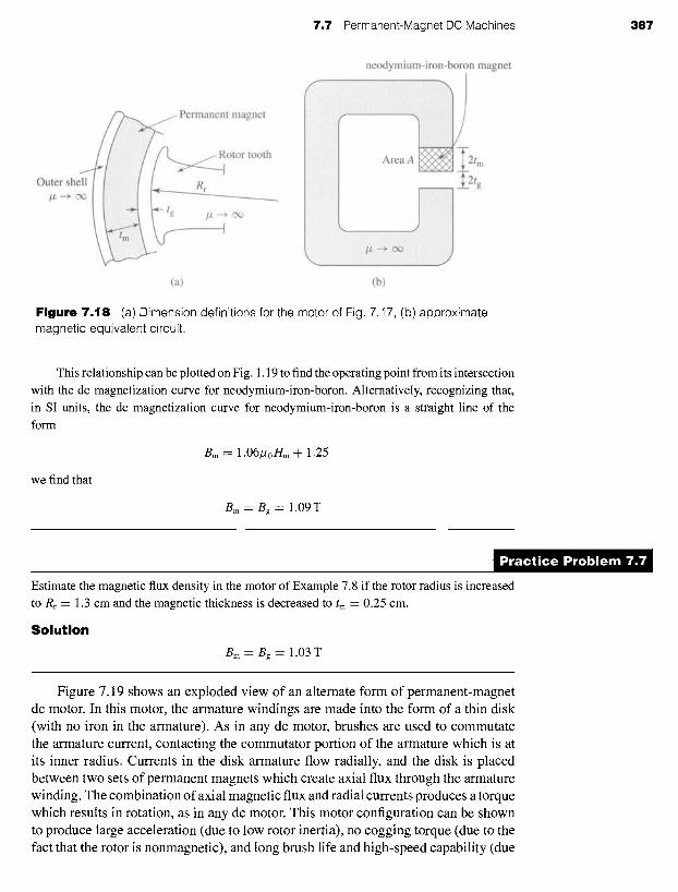
Figure 7.18a defines the dimensions of a permanent-magnet dc motor similar to that of Fig. 7.17.
Assume the following values:
Rotor radius Rr -- 1.2 cm
Gap length tg = 0.05 cm
Magnet thickness tm = 0.35 cm
Also assume that both the rotor and outer shell are made of infinitely permeable magnetic
material (# ~ c¢) and that the magnet is neodymium-iron-boron (see Fig. 1.19).
Ignoring the effects of rotor slots, estimate the magnetic flux density B in the air gap of
this motor.
I I S o l u t i o n Because the rotor and outer shell are assumed to be made of material with infinite magnetic
permeability, the motor can be represented by a magnetic equivalent circuit consisting of an
air gap of length 2tg in series with a section of neodymium-iron-boron of length 2tm (see
Fig. 7.18b). Note that this equivalent circuit is approximate because the cross-sectional area of
the flux path in the motor increases with increasing radius, whereas it is assumed to be constant
in the equivalent circuit.
The solution can be written down by direct analogy with Example 1.9. Replacing the
air-gap length g with 2tg and the magnet length lm with 2tm, the equation for the load line can
be written as
Bm -- -/z0 n m = - 7 # 0 n m
7.7 Permanent-Magnet DC Machines 387
neodymium-iron-boron magnet
t magnet
Outer she /z --+ c
otor tooth
~CX~
2tm
2tg
(a) (b)
Figure 7.18 (a) Dimension definitions for the motor of Fig. 7.17, (b) approximate magnetic equivalent circuit.
This relationship can be plotted on Fig. 1.19 to find the operating point from its intersection
with the dc magnetization curve for neodymium-iron-boron. Alternatively, recognizing that,
in SI units, the dc magnetization curve for neodymium-iron-boron is a straight line of the form
Bm = 1.06#oHm + 1.25
we find that
Bm= Bg -- 1.09 T
) rac t ice Problem 7 .
Estimate the magnetic flux density in the motor of Example 7.8 if the rotor radius is increased
to Rr -- 1.3 cm and the magnetic thickness is decreased to tm = 0.25 cm.
Solut ion
Bm = Bg ----- 1.03 T
Figure 7.19 shows an exploded view of an alternate form of permanent-magnet dc motor. In this motor, the armature windings are made into the form of a thin disk
(with no iron in the armature). As in any dc motor, brushes are used to commutate
the armature current, contacting the commutator portion of the armature which is at
its inner radius. Currents in the disk armature flow radially, and the disk is placed between two sets of permanent magnets which create axial flux through the armature winding. The combination of axial magnetic flux and radial currents produces a torque
which results in rotation, as in any dc motor. This motor configuration can be shown
to produce large acceleration (due to low rotor inertia), no cogging torque (due to the
fact that the rotor is nonmagnetic), and long brush life and high-speed capability (due
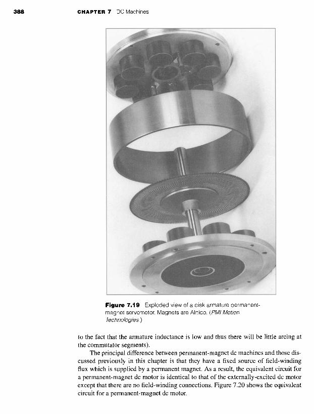
388 CHAPTER 7 DC Machines
F igure 7.19 Exploded view of a disk armature permanent- magnet servomotor. Magnets are Alnico. (PMI Motion Technologies.)
to the fact that the armature inductance is low and thus there will be little arcing at the commutator segments).
The principal difference between permanent-magnet dc machines and those dis- cussed previously in this chapter is that they have a fixed source of field-winding flux which is supplied by a permanent magnet. As a result, the equivalent circuit for a permanent-magnet dc motor is identical to that of the externally-excited dc motor except that there are no field-winding connections. Figure 7.20 shows the equivalent circuit for a permanent-magnet dc motor.

7.7 Permanent-Magnet DC Machines 389
Ia R a
o------~ , V ~ +
V t Ea = Kmogm
0
Figure 7 .20 Equivalent circuit of a permanent-magnet dc motor.
From Eq. 7.14, the speed-voltage term for a dc motor can be written in the form Ea = Ka~dCOm where ~a is the net flux along the field-winding axis and Ka is a geometric constant. In a permanent-magnet dc machine, ~a is constant and thus Eq. 7.14 can be reduced to
E a - - Kmogm (7.26)
where
Km = Ka~d (7.27)
is known as the torque constant of the motor and is a function of motor geometry and magnet properties.
Finally the torque of the machine can be easily found from Eq. 7.16 as
Eala Tmech- = Kmla (7.28)
O)m
In other words, the torque of a permanent magnet motor is given by the product of the torque constant and the armature current.
" X A M P L E 7.!
A permanent-magnet dc motor is known to have an armature resistance of 1.03 g2. When operated at no load from a dc source of 50 V, it is observed to operate at a speed of 2100 r/min and to draw a current of 1.25 A. Find (a) the torque constant Km, (b) the no-load rotational losses of the motor and (c) the power output of the motor when it is operating at 1700 r/min from a 48-V source.
I I S o l u t i o n a. From the equivalent circuit of Fig. 7.20, the generated voltage Ea can be found as
Ea = V t - I a R a
= 5 0 - 1.25 × 1.03 = 48.7 V
At a speed of 2100 r/min,
( 2 1 0 0 r ) ( 2 r r r a d ) ( 1 man) 09 m - " X X
min 60 s
= 220 rad/sec

390 CHAPTER 7 DC Machines
Therefore, from Eq. 7.26,
Ea 48.7 Km = - - = 0 . 2 2 V/(rad/sec)
O) m 2 2 0
b. At no load, all the power supplied to the generated voltage Ea is used to supply rotational
losses. Therefore
Rotational losses = Eala "-- 48.7 x 1.25 = 61 W
c. At 1700 r/min,
O.) m = 1700 = 178 rad/sec
and
Ea = Km(.Om = 0.22 x 178 = 39.2 V
The input current can now be found as
Vt - Ea 4 8 - 3 9 . 2 / a = - -
Ra 1.03 = 8.54 A
The electromagnetic power can be calculated as
Pmech =-- Eala -- 39.2 X 8.54 = 335 W
Assuming the rotational losses to be constant at their no-load value (certainly an
approximation), the output shaft power can be calculated:
P s h a f t - - P m e c h - - rotational losses = 274 W
The armature resistance of a small dc motor is measured to be 178 mr2. With an applied voltage
of 9 V, the motor is observed to operate at a no-load speed of 14,600 r/min while drawing a
current of 437 mA. Calculate (a) the rotational loss and (b) the motor torque constant Kin.
S o l u t i o n
a. Rotational loss = 3.90 W
b. Km = 5.84 x 10 .3 V/(rad/sec)
7.8 C O M M U T A T I O N A N D I N T E R P O L E S One of the most important l imiting factors on the sat isfactory operat ion of a dc machine
is the ability to t ransfer the necessary armature current through the brush contact at the
commuta to r wi thout sparking and wi thout excess ive local losses and heating of the
brushes and commutator . Sparking causes destruct ive blackening, pitting, and wear
of both the commuta to r and the brushes, condi t ions which rapidly become worse
and burn away the copper and carbon. Sparking may be caused by faulty mechanical
7,8 Commutation and Interpoles 39t
conditions, such as chattering of the brushes or a rough, unevenly worn commutator, or, as in any switching problem, by electrical conditions. The latter conditions are seriously influenced by the armature mmf and the resultant flux wave.
As indicated in Section 7.2, a coil undergoing commutation is in transition be- tween two groups of armature coils: at the end of the commutation period, the coil cur- rent must be equal but opposite to that at the beginning. Figure 7.7b shows the armature in an intermediate position during which the coils in slots 1 and 7 are being commu- tated. The commutated coils are short-circuited by the brushes. During this period the brushes must continue to conduct the armature current Ia from the armature winding to the external circuit. The short-circuited coil constitutes an inductive circuit with time- varying resistances at the brush contact, with rotational voltages induced in the coil, and with both conductive and inductive coupling to the rest of the armature winding.
The attainment of good commutation is more an empirical art than a quantitative science. The principal obstacle to quantitative analysis lies in the electrical behavior of the carbon-copper (brush-commutator) contact film. Its resistance is nonlinear and is a function of current density, current direction, temperature, brush material, moisture, and atmospheric pressure. Its behavior in some respects is like that of an ionized gas or plasma. The most significant fact is that an unduly high current density in a portion of the brush surface (and hence an unduly high energy density in that part of the contact film) results in sparking and a breakdown of the film at that point. The boundary film also plays an important part in the mechanical behavior of the rubbing surfaces. At high altitudes, definite steps must be taken to preserve it, or extremely-rapid brush wear takes place.
The empirical basis of securing sparkless commutation, then, is to avoid excessive current densities at any point in the copper-carbon contact. This basis, combined with the principle of utilizing all material to the fullest extent, indicates that optimum conditions are obtained when the current density is uniform over the brush surface during the entire commutation period. A linear change of current with time in the commutated coil, corresponding to linear commutation as shown in Fig. 7.8, brings about this condition and is accordingly the optimum.
The principal factors tending to produce linear commutation are changes in brush- contact resistance resulting from the linear decrease in area at the trailing brush edge and linear increase in area at the leading edge. Several electrical factors mitigate against linearity. Resistance in the commutated coil is one example. Usually, however, the voltage drop at the brush contacts is sufficiently large (of the order of 1.0 V) in comparison with the resistance drop in a single armature coil to permit the latter to be ignored. Coil inductance is a much more serious factor. Both the voltage of self-induction in the commutated coil and the voltage of mutual-induction from other coils (particularly those in the same slot) undergoing commutation at the same time oppose changes in current in the commutated coil. The sum of these two voltages is often referred to as the reactance voltage. Its result is that current values in the short- circuited coil lag in time the values dictated by linear commutation. This condition is known as undercommutation or delayed commutation.
Armature inductance thus tends to produce high losses and sparking at the trailing brush tip. For best commutation, inductance must be held to a minimum by using the fewest possible number of turns per armature coil and by using a multipolar design

392 CHAPTER 7 DC Machines
with a short armature. The effect of a given reactance voltage in delaying commutation is minimized when the resistive brush-contact voltage drop is significant compared with it. This fact is one of the main reasons for the use of carbon brushes with their appreciable contact drop. When good commutation is secured by virtue of resistance drops, the process is referred to as resistance commutation. It is typically used as the exclusive means only in fractional-horsepower machines.
Another important factor in the commutation process is the rotational voltage in- duced in the short-circuited coil. Depending on its sign, this voltage may hinder or aid commutation. In Fig. 7.11, for example, cross-magnetizing armature reaction creates a definite flux in the interpolar region. The direction of the corresponding rotational voltage in the commutated coil is the same as the current under the immediately pre- ceding pole face. This voltage then encourages the continuance of current in the old direction and, like the resistance voltage, opposes its reversal. To aid commutation, the rotational voltage must oppose the reactance voltage. The general principle is to produce in the coil undergoing commutation a rotational voltage which approxi- mately compensates for the reactance voltage, a principle called voltage commutation. Voltage commutation is used in almost all modern integral-horsepower commutating machines. The appropriate flux density is introduced in the commutating zone by means of small, narrow poles located between the main poles. These auxiliary poles are called interpoles or commutating poles.
The general appearance of interpoles and an approximate map of the flux pro- duced when they alone are excited are shown in Fig. 7.21. The interpoles are the smaller poles between the larger main poles in the dc-motor section shown in Fig. 7.23. The polarity of a commutating pole must be that of the main pole just ahead of it, i.e., in the direction of rotation for a generator, and just behind it for a motor. The interpole mmf must be sufficient to neutralize the cross-magnetizing armature mmf in the in- terpolar region and enough more to furnish the flux density required for the rotational voltage in the short-circuited armature coil to cancel the reactance voltage. Since both the armature mmf and the reactance voltage are proportional to the armature current, the commutating winding must be connected in series with the armature. To preserve the desired linearity, the commutating pole should operate at a relatively low flux level. By the use of commutating fields sparkless commutation can be obtained over a wide range in large dc machines. In accordance with the performance standards
Interpole { leakage flux
Effect ive(~/ \ interpole flux
............................................................... Field ~ I ) iron
i Commutating or : i ~ Field interpole winding
j ~ii~ pole ~ . £ Z ~ ' !i~ii!i!iiiil iliii
" .....E-, Commutating ~, pole or interpole
Armature iron
Figure 7 . 2 1 Interpoles and their assoc ia ted c o m p o n e n t flux.

7.9 Compensating Windings 393
of NEMA, 1 general-purpose dc machines must be capable of carrying for one minute, with successful commutation, loads of 150 percent of the current corresponding to their continuous rating when operating with a field current equal to their rated-load excitation.
7.9 C O M P E N S A T I N G W I N D I N G S For machines subjected to heavy overloads, rapidly changing loads, or operation with a weak main field, there is the possibility of trouble other than simply sparking at the brushes. At the instant when an armature coil is located at the peak of a badly distorted flux wave, the coil voltage may be high enough to break down the air between the adjacent segments to which the coil is connected and result in flashover, or arcing, between segments. The breakdown voltage here is not high, because the air near the commutator is in a condition favorable to breakdown, due to the presence of the plasma carrying the armature current between the brushes and the commutator. The maximum allowable voltage between segments is of the order of 30 to 40 V, a fact which limits the average voltage between segments to lower values and thus determines the minimum number of segments which can be used in a proposed design. Under transient conditions, high voltages between segments may result from the induced voltages associated with growth and decay of armature flux. Inspection of Fig. 7.10, for instance, may enable one to visualize very appreciable voltages of this nature being induced in a coil under the pole centers by the growth or decay of the armature flux shown in the sketch. Consideration of the sign of this induced voltage will show that it adds to the normal rotational emf when load is dropped from a generator or added to a motor. Flashing between segments may quickly spread around the entire commutator and, in addition to its possibly destructive effects on the commutator, constitutes a direct short circuit on the line. Even with interpoles present, therefore, armature reaction under the poles definitely limits the conditions under which a machine can operate.
These limitations can be considerably extended by compensating or neutralizing the armature mmf under the pole faces. Such compensation can be achieved by means of a compensating or pole-face winding (Fig. 7.22) embedded in slots in the pole face and having a polarity opposite to that of the adjoining armature winding. The physical appearance of such a winding can be seen in the stator section of Fig. 7.23. Since the axis of the compensating winding is the same as that of the armature, it will almost completely neutralize the armature reaction of the armature conductors under the pole faces when it is given the proper number of turns. It must be connected in series with the armature in order to carry a proportional current. The net effect of the main field, armature, commutating winding, and compensating winding on the air-gap flux is that, except for the commutation zone, the resultant flux-density distribution is substantially the same as that produced by the main field alone (Fig. 7.11). Furthermore, the addition
1 NEMA Standards Publication No. MG1-1998, Motors and Generators, Sections 23 and 24, National Electrical Manufactures Association, 300 North 17th Street, Suite 1847, Rosslyn, Virginia, 22209.

394 CHAPTER 7 DC Machines
Commutating field or interpole
Figure 7 .22 Section of dc machine showing compensating winding.
of a compensating winding improves the speed of response of the machine because it reduces the armature-circuit time constant.
The main disadvantage of pole-face windings is their expense. They are used in machines designed for heavy overloads or rapidly-changing loads (steel-mill motors are a good example of machines subjected to severe duty cycles) or in motors intended to operate over wide speed ranges by shunt-field control. By way of a schematic summary, Fig. 7.24 shows the circuit diagram of a compound machine with a com- pensating winding. The relative position of the coils in this diagram indicates that the commutating and compensating fields act along the armature axis, and the shunt and
:~:i:, :ii~iiiii~!ii::i~i;ii~;i!ii ~ ,hi~i~i:i~i:i~!~:i,i~:i~i
:~:ii~? : ~ ....... :::iiiiiiiiiiiiiiiiiiiiiiiiiiii Yi~ii!ii~!iiiiiiililiiiiiiiiiii!~i~:i :~ii,iiii~iii!i!i!iiG,i:!::,: ~
~:!!i!i~iii~ii!i!~i,~'i! ~I~ ~I:II~! ;~:~,:~::,,:U:::::~,;; L: ~
~ ~:i ~?iiiiii!ii~ i ~ i~:i:~: ,~
~ii!~!i ~!~ii~!~:ilil ~II!?~: YI,~I ~:' ~(i :~ , i "
..... ~!!~::i ~ _?~:
Figure 7 .23 Section of a dc motor stator showing shunt and series coils, interpoles and pole-face compensating winding. (Westinghouse Electric Company.)

7.10 Series Universal Motors 395
o Tshunt / field t_00_0 ,
Field ~
o rheostat ~
&9.L Series field
Commutating winding
( ~ Armature
o Compensating o winding
Figure 7.24 Schematic connection diagram of a dc machine.
series fields act along the axis of the main poles. Rather complete control of air-gap flux around the entire armature periphery is thus achieved.
7 .10 SERIES U N I V E R S A L M O T O R S Figure 7.25 shows a dc machine connection with a series-connected field winding. For this connection the direct-axis flux @d is proportional to the armature current. Hence from Eq. 7.14, the generated voltage Ea is proportional to the product of the armature current and the motor speed, and from Eq. 7.16 we see that the torque will be proportional to the square of the armature current.
The dashed line in Fig. 7.26 shows a typical speed-torque characteristic for such a series-connected motor under dc operating conditions. Note that because the torque is proportional to the square of the armature current, the torque depends only upon the magnitude of the armature voltage and not its polarity; reversing the polarity of the applied voltage will not change the magnitude or direction of the applied torque.
If the rotor and stator structures of a series connected motor are properly laminated to reduce ac eddy-current losses, the resultant motor is referred to as a series universal
motor. The series universal motor has the convenient ability to run on either alternating or direct current and with similar characteristics. Such a single-phase series motor therefore is commonly called a universal motor. The torque angle is fixed by the brush position and is normally at its optimum value of 90 ° . If alternating current is supplied to a series universal motor, the torque will always be in the same direction, although it will pulsate in magnitude at twice line frequency. Average torque will be produced, and the performance of the motor will be generally similar to that with direct current.
Series Ia field
>
+
Va Ea
O
Armature
Figure 7.25 Series-connected universal machine.

396 CHAPTER 7 DC Machines
400
300
E o : 200 ~9
100
\ . i
60 Hz i J
J i
20 40
\ dc
" " ' 4
60 80 1 O0 Percent rated speed
Figure 7.26 Typical torque-speed characteristics of a series universal motor.
Small universal motors are used where light weight is important, as in vac- uum cleaners, kitchen appliances, and portable tools, and usually operate at high speeds (1500 to 15,000 r/min). Typical characteristics are shown in Fig. 7.26. The ac and dc characteristics differ somewhat for two reasons: (1) With alternating current, reactance-voltage drops in the field and armature absorb part of the applied voltage; therefore for a specified current and torque the rotational counter emf generated in the armature is less than with direct current, and the speed tends to be lower. (2) With alternating current, the magnetic circuit may be appreciably saturated at the peaks of the current wave. Thus the rms value of the flux may be appreciably less with alternat- ing current than with the same rms value of direct current. The torque therefore tends to be less with alternating than with direct current. The universal motor provides the highest horsepower per dollar in the fractional-horsepower range, at the expense of noise, relatively short life, and high speed.
To obtain control of the speed and torque of a series universal motor, the applied ac voltage may be varied by the use of a Triac, such as is discussed in Chapter 10. The firing angle of the Triac can be manually adjusted, as in a trigger-controlled electric drill, or it can be controlled by a speed control circuit, as in some portable tools and appliances. The combination of a series motor and a solid-state device provides an economical, controllable motor package.
7.11 S U M M A R Y This chapter has discussed the significant operating characteristics of dc machines. In general, the outstanding advantage of dc machines lies in their flexibility and versatility. Before the widespread availability of ac motor drives, dc machines were essentially the only choice available for many applications which required a high degree of control. Their principal disadvantages stem from the complexity associated with the armature winding and the commutator/brush system. Not only does this additional complexity increase the cost over competing ac machines, it also increases the need for maintenance and reduces the potential reliability of these machines. Yet the advantages of dc motors remain, and they continue to retain a strong competitive position in both large sizes for industrial applications and in smaller sizes for a wide variety of applications.
7.12 Problems 397
Dc generators are a simple solution to the problem of converting mechanical energy to electric energy in dc form, although ac generators feeding rectifier systems are certainly an option which must be considered. Among dc generators themselves, separately-excited and cumulatively-compounded, self-excited machines are the most common. Separately-excited generators have the advantage of permitting a wide range of output voltages, whereas self-excited machines may produce unstable voltages at lower output voltages where the field-resistance line becomes essentially tangent to the magnetization curve. Cumulatively-compounded generators may produce a substantially flat voltage characteristic or one which rises with load, whereas shunt- or separately-excited generators may produce a drooping voltage characteristic unless external regulating means (such as a series field winding) are added.
Among dc motors, the outstanding characteristics of each type are as follows. The series motor operates with a decidedly drooping speed as load is added, the no-load speed usually being prohibitively high; the torque is proportional to almost the square of the current at low flux levels and to some power between 1 and 2 as saturation increases. The shunt motor at constant field current operates at a slightly drooping but almost constant speed as load is added, the torque being almost proportional to armature current; equally important, however, is the fact that its speed can be controlled over wide ranges by shunt-field control, armature-voltage control, or a combination of both. Depending on the relative strengths of the shunt and series field, the cumulatively-compounded motor is intermediate between the other two and may be given essentially the advantages of one or the other.
In a wide variety of low-power applications in systems which are run from a dc source (automotive applications, portable electronics, etc.), dc machines are the most cost-effective choice. These dc machines are constructed in a wide-range of configurations, and many of them are based upon permanent-magnet excitation. In spite of the wide variety of dc machines which can be found in these various applica- tions, their performance can readily be determined using the models and techniques presented in this chapter.
7 .12 P R O B L E M S 7.1 Consider a separately-excited dc motor. Describe the speed variation of the
motor operating unloaded under the following conditions:
a. The armature terminal voltage is varied while the field current is held constant.
b. The field current is varied while the armature terminal voltage is held constant.
c. The field winding is connected in shunt directly to the armature terminals, and the armature terminal voltage is then varied.
7.2 A dc shunt motor operating at an armature terminal voltage of 125 V is observed to be operating at a speed of 1180 r/min. When the motor is operated unloaded at the same armature terminal voltage but with an additional resistance of 5 f2 in series with the shunt field, the motor speed is observed to be 1250 r/min.

3 9 8 C H A P T E R 7 DC Mach ines
a. Calculate the resistance of the series field.
b. Calculate the motor speed which will result if the series resistance is increased from 5 f2 to 15 f2.
7.3 For each of the following changes in operating condition for a dc shunt motor, describe how the armature current and speed will vary:
a. Halving the armature terminal voltage while the field flux and load torque remain constant.
b. Halving the armature terminal voltage while the field current and load power remain constant.
c. Doubling the field flux while the armature terminal voltage and load torque remain constant.
d. Halving both the field flux and armature terminal voltage while the load power remains constant.
e. Halving the armature terminal voltage while the field flux remains constant and the load torque varies as the square of the speed.
Only brief quantitative statements describing the general nature of the effect are required, for example, "speed approximately doubled."
7.4 The constant-speed magnetization curve for a 25-kW, 250-V dc machine at a speed of 1200 r/min is shown in Fig. 7.27. This machine is separately excited and has an armature resistance of 0.14 f2. This machine is to be operated as a dc generator while driven from a synchronous motor at constant
speed.
a. What is the rated armature current of this machine?
b. With the generator speed held at 1200 r/min and if the armature current is limited to its rated value, calculate the maximum power output of the
300
250
> 200
E ~D
150 ~D
100 r~
50
0 0
. . . . . . . . . . . . . . . . . . . . . . . . . . . . . . . . . . . . . . . . . . . . . . . . . . . . . . . . . . . . . . . . . . . . . . . . . . . . . . . . . . . . . . . . . . . . .
........................ I I
0.5 1.0 1.5 2.0 2.5 Field current, A
F i g u r e 7.27 1200 r/min magnetization curve for the dc generator of Problem 7.4.
7,12 Problems 399
generator and the corresponding armature voltage for constant field currents of (i) 1.0 A, (ii) 2.0 A and (iii) 2.5 A.
c. Repeat part (b) if the speed of the synchronous generator is reduced to 900 r/min.
7.5 The dc generator of Problem 7.4 is to be operated at a constant speed of 1200 r/min into a load resistance of 2.5 f2.
a. Using the "spline0" function of MATLAB and the points of the magnetization curve of Fig. 7.27 at 0, 0.5, 1.0, 1.5, 2.0, and 2.5 A, create a MATLAB plot of the magnetization curve of Fig. 7.27.
b. Using the "spline0" function as in part (a), use MATLAB to plot (i) the terminal voltage and (ii) the power delivered to the load as the generator field current is varied from 0 to 2.5 A.
7.6 The dc machine of Problem 7.4 is to be operated as a motor supplied by a constant armature terminal voltage of 250 V. If saturation effects are ignored, the magnetization curve of Fig. 7.27 becomes a straight line with a constant slope of 150 volts per ampere of field current. For the purposes of this problem, you may assume that saturation effects can be neglected.
a. Assuming that the field current is held constant at 1.67 A, plot the motor speed as a function of motor shaft power as the shaft power varies from 0 to 25 kW.
b. Now assuming that the field current can be adjusted in order to maintain the motor speed constant at 1200 r/min, plot the required field current as a function of motor shaft power as the shaft power varies from 0 to 25 kW.
7.7 Repeat Problem 7.6 including the saturation effects represented by the saturation curve of Fig. 7.27. For part (a), set the field current equal to the value required to produce an open-circuit armature terminal voltage of 250 V at 1200 r/min. (Hint: This problem is most easily solved using MATLAB and its "spline0" function as in Problem 7.5.)
7.8 A 15-kW, 250-V, 1150 r/min shunt generator is driven by a prime mover whose speed is 1195 r/min when the generator delivers no load. The speed falls to 1140 r/min when the generator delivers 15 kW and may be assumed to decrease in proportion to the generator output. The generator is to be changed into a short-shunt compound generator by equipping it with a series field winding which will cause its voltage to rise from 230 V at no load to 250 V for a load of 61.5 A. It is estimated that the series field winding will have a resistance of 0.065 S2. The armature resistance (including brushes) is 0.175 f2. The shunt field winding has 500 turns per pole.
To determine the necessary series-field turns, the machine is run as a separately-excited generator and the following load data are obtained:
Armature terminal voltage = 254 V
Armature current = 62.7 A

4 0 0 C H A P T E R 7 DC Machines
Field current = 1.95 A
Speed = 1140 r/min
The magnetization curve at 1195 r/min is as follows:
Ea, V 230 240 250 260 270 280
Ir, A 1.05 1.13 1.25 1.44 1.65 1.91
Determine
a. the armature reaction in equivalent demagnetizing ampere-turns per pole for Ia = 62.7 A and
b. the necessary number of series-field turns per pole.
(Hint: This problem can be solved either graphically or by use of the MATLAB "spline()" function to represent the magnetization curve.)
7.9 When operated from a 230-V dc supply, a dc series motor operates at 975 r/min with a line current of 90 A. Its armature-circuit resistance is 0.11 f2 and its series-field resistance is 0.08 f2. Due to saturation effects, the flux produced by an armature current of 30 A is 48 percent of that at an armature current of 90 A. Find the motor speed when the armature voltage is 230 V and the armature current is 30 A.
7.10 Consider the long-shunt, 250-V, 100-kW dc machine of Example 7.3. Assuming the machine is operated as a motor at a constant supply voltage of 250-V with a constant shunt-field current of 5.0 A, use MATLAB to plot the motor speed as a function of load. Use the MATLAB "spline()" function to represent the magnetization curve of Fig. 7.14. Neglect armature-reaction effects. Include two plots, one for the case where the series-field ampere-turns add to those of the shunt field and the second for the case where the series-field ampere-turns oppose those of the shunt field.
7.11 A 250-V dc shunt-wound motor is used as an adjustable-speed drive over the range from 0 to 2000 r/min. Speeds from 0 to 1200 r/min are obtained by adjusting the armature terminal voltage from 0 to 250 V with the field current kept constant. Speeds from 1200 r/min to 2000 r/min are obtained by decreasing the field current with the armature terminal voltage remaining at 250 V. Over the entire speed range, the torque required by the load remains constant.
a. Sketch the general form of the curve of armature current versus speed over the entire range. Ignore machine losses and armature-reaction effects.
b. Suppose that, instead of operating with constant torque, the load torque at any given speed is adjusted to maintain the armature current at its rated value. Sketch the general form of the allowable torque as a function of speed assuming the motor is controlled as described above.
7.12 Two adjustable-speed dc shunt motors have maximum speeds of 1800 r/min and minimum speeds of 500 r/min. Speed adjustment is obtained by
7.12 Problems 401
field-rheostat control. Motor A drives a load requiring constant power over the speed range; motor B drives one requiring constant torque. All losses and armature reaction may be neglected.
a. If the power outputs of the two motors are equal at 1800 r/min and the armature currents are each 125 A, what will the armature currents be at 500 r/min?
b. If the power outputs of the two motors are equal at 500 r/min and the armature currents are each 125 A, what will the armature current be at 1800 r/min?
c. Answer parts (a) and (b) with speed adjustment by armature-voltage control with conditions otherwise the same.
7.13 Consider a dc shunt motor connected to a constant-voltage source and driving a load requiring constant electromagnetic torque. Show that if Ea > 0.5Vt (the normal situation), increasing the resultant air-gap flux decreases the speed, whereas if Ea < 0.5 Vt (as might be brought about by inserting a relatively high resistance in series with the armature), increasing the resultant air-gap flux increases the speed.
7.14 A separately-excited dc motor is mechanically coupled to a three-phase, four-pole, 30-kVA, 460-V, cylindrical-pole synchronous generator. The dc motor is connected to a constant 230-V dc supply, and the ac generator is connected to a 460-V, fixed-voltage, fixed-frequency, three-phase supply. The synchronous reactance of the synchronous generator is 5.13 f2/phase. The armature resistance of the dc motor is 30 mA. The four-pole dc machine is rated 30 kW at 230 V. All unspecified losses are to be neglected.
a. If the two machines act as a motor-generator set receiving power from the dc source and delivering power to the ac supply, what is the excitation voltage of the ac machine in volts per phase (line-to-neutral) when it delivers 30 kW at unity power factor? What is the internal voltage of the dc motor?
b. Leaving the field current of the ac machine at the value corresponding to the condition of part (a), what adjustment can be made to reduce the power transfer between the two machines to zero? Under this condition of zero power transfer, what is the armature current of the dc machine? What is the armature current of the ac machine?
c. Leaving the field current of the ac machine as in parts (a) and (b), what adjustment can be made to cause the transfer of 30 kW from the ac source to the dc source? Under these conditions what are the armature current and internal voltage of the dc machine? What will be the magnitude and phase of the current of the ac machine?
7.15 A 150-kW, 600-V, 600 r/min dc series-wound railway motor has a combined field and armature resistance (including brushes) of 0.125 f2. The full-load current at rated voltage and speed is 250 A. The magnetization curve at 400 r/min is as follows:
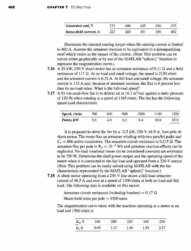
4 0 2 C H A P T E R 7 DC Machines
Generated emf, V 375 400 425 450 475
Series-field current, A 227 260 301 350 402
Determine the internal starting torque when the starting current is limited to 460 A. Assume the armature reaction to be equivalent to a demagnetizing mmf which varies as the square of the current. (Hint: This problem can be solved either graphically or by use of the MATLAB "spline0" function to represent the magnetization curve.)
7.16 A 25-kW, 230-V shunt motor has an armature resistance of 0.11 ~2 and a field resistance of 117 ~. At no load and rated voltage, the speed is 2150 r/min and the armature current is 6.35 A. At full load and rated voltage, the armature current is 115 A and, because of armature reaction, the flux is 6 percent less than its no-load value. What is the full-load speed?
7.17 A 91-cm axial-flow fan is to deliver air at 16.1 m3/sec against a static pressure of 120 Pa when rotating at a speed of 1165 r/min. The fan has the following speed-load characteristic
Speed, r/rain 700 800 900 1000 1100 1200
Power, kW 3.6 4.9 6.5 8.4 10.8 13.9
It is proposed to drive the fan by a 12.5 kW, 230-V, 46.9-A, four-pole dc shunt motor. The motor has an armature winding with two parallel paths and Ca = 666 active conductors. The armature-circuit resistance is 0.215 ~. The armature flux per pole is ~d = 10 -2 Wb and armature reaction effects can be neglected. No-load rotational losses (to be considered constant) are estimated to be 750 W. Determine the shaft power output and the operating speed of the motor when it is connected to the fan load and operated from a 230-V source. (Hint: This problem can be easily solved using MATLAB with the fan characteristic represented by the MATLAB "spline()" function.)
7.18 A shunt motor operating from a 230-V line draws a full-load armature current of 46.5 A and runs at a speed of 1300 r/min at both no load and full load. The following data is available on this motor:
Armature-circuit resistance (including brushes) = 0.17 f2
Shunt-field turns per pole -- 1500 turns
The magnetization curve taken with the machine operating as a motor at no load and 1300 r/min is
E,, V 180 200 220 240 250
It., A 0.98 1.15 1.46 1.93 2.27

7.12 Problems 403
a. Determine the shunt-field current of this motor at no load and 1300 r/min when connected to a 230-V line. Assume negligible armature-circuit resistance and armature reaction at no load.
b. Determine the effective armature reaction at full load in ampere-turns per pole.
c. How many series-field turns should be added to make this machine into a long-shunt cumulatively compounded motor whose speed will be 1210 r/min when the armature current is 46.5 A and the applied voltage is 230 V? Assume that the series field has a resistance of 0.038 f2.
d. If a series-field winding having 20 turns per pole and a resistance of 0.038 f2 is installed, determine the speed when the armature current is 46.5 A and the applied voltage is 230 V.
(Hint: This problem can be solved either graphically or by use of the MATLAB "spline0" function to represent the magnetization curve.)
7.19 A 7.5-kW, 230-V shunt motor has 2000 shunt-field turns per pole, an armature resistance (including brushes) of 0.21 f2, and a commutating-field resistance of 0.035 f2. The shunt-field resistance (exclusive of rheostat) is 310 f2. When the motor is operated at no load with rated terminal voltage and varying shunt-field resistance, the following data are obtained:
Speed, r/min 1110 1130 1160 1200 1240
if, A 0.672 0.634 0.598 0.554 0.522
The no-load armature current is negligible. When the motor is operating at full load and rated terminal voltage with a field current of 0.554 A, the armature current is 35.2 A and the speed is 1185 r/min.
a. Calculate the full-load armature reaction in equivalent demagnetizating ampere-turns per pole.
b. Calculate the full-load electromagnetic torque at this operating condition.
c. What starting torque will the motor produce with maximum field current if the starting armature current is limited to 65 A? Assume that the armature reaction under these conditions is equal to 160 ampere-turns per pole.
d. Design a series field winding to give a speed of 1050 r/min when the motor is loaded to an armature current of 35.2 A and when the shunt field current is adjusted to give a no-load speed of 1200 r/min. Assume the series field will have a resistance of 0.05 f2.
(Hint: This problem can be solved either graphically or by use of the MATLAB "spline0" function to represent the magnetization curve.)
7.20 When operated at rated voltage, a 230-V shunt motor runs at 1750 r/min at full load and at no load. The full-load armature current is 70.8 A. The shunt field winding has 2000 turns per pole. The resistance of the armature circuit

4 0 4 CHAPTER 7 DC Machines
(including brushes and interpoles) is 0.15 f2. The magnetization curve at 1750 r/min is
E,, V 200 210 220 230 240 250
It,, A 0.40 0.44 0.49 0.55 0.61 0.71
a. Compute the demagnetizing effect of the armature reaction at full load.
b. A long-shunt cumulative series field winding having four turns per pole and a resistance of 0.038 f2 is added to the machine. Compute the speed at full-load current and rated voltage. The shunt field current will remain equal to that of part (a).
c. With the series-field winding of part (b) installed, compute the internal starting torque in N. m if the starting armature current is limited to 125 A. Assume that the corresponding demagnetizating effect of armature reaction is 230 ampere-turns per pole.
(Hint: This problem can be solved either graphically or by use of the MATLAB "spline0" function to represent the magnetization curve.)
7.21 A 230-V dc shunt motor has an armature-circuit resistance of 0.23 f2. When operating from a 230-V supply and driving a constant-torque load, the motor is observed to be drawing an armature current of 60 A. An external resistance of 1.0 f2 is now inserted in series with the armature while the shunt field current is unchanged. Neglecting the effects of rotational losses and armature reaction, calculate
a. the resultant armature current and
b. the fractional speed change of the motor.
7.22 A common industrial application of dc series motors is in crane and hoist drives. This problem relates to the computation of selected motor performance characterstics for such a drive. The specific motor concerned is a series-wound, 230-V, totally-enclosed motor having a 1/2-hour crane rating of 100 kW with a 75°C temperature rise. The performance characteristics
T a b l e 7.1 Motor characteristics for Problem 7.22.
Line current Shaft torque Speed A N. m r/min
100 217 940 200 570 630 300 1030 530 400 1480 475 500 1980 438 600 2470 407 700 3000 385 800 3430 370

7.12 Problems 405
Series R2 Field
(a) (b)
Figure 7.28 Series crane motor (Problem 7.22): (a) hoisting connection and (b) lowering connection.
of the motor alone at 230 V as found in the manufacturer's catalog are listed in Table 7.1. The resistance of the armature (including brushes) plus commutating winding is 0.065 ~ and that of the series field winding is 0.027 ~. Armature reaction effects can be ignored.
The motor is to be connected as in Fig. 7.28a for hoisting and Fig. 7.28b for lowering. The former connection consists simply of series-resistance control. The latter connection provides dynamic breaking with the field reconnected in shunt with the addition of an adjustable series resistance.
You will use MATLAB to plot some sample speed-torque curves (speed as a function of torque) to determine the suitability of the motor and control for the specified application. Plot all of the curves on a single set of axes coveting roughly the torque-magnitude range found in Table 7.1. Provide for both positive and negative values of speed, corresponding respectively to hoisting and lowering, as well as for both positive and negative values of torque, corresponding respectively to torque in the direction of raising the load and torque in the direction of lowering the load.
a. For the hoisting connection, plot speed-torque curves for the control resistor Rc set at 0, 0.3 and 0.6 f2. If any of these curves extend into the fourth quadrant within the range of torques covered, interpret physically what operation in that regime means.
b. For the lowering connection, plot a speed-torque curve for R1 = 0.3 f2 and R2 = 0.3 f2. The most important portion of this curve is in the fourth quadrant, but if it extends into the third quadrant, that region should also be plotted and interpreted physically.
c. In part (b), what is the lowering speed corresponding to a torque of 1500 N. m? (Hint: This can be found easily using the MATLAB "spline0" function.)
7.23 A 25-kW, 230-V shunt motor has an armature resistance of 0.064 f2 and a field-circuit resistance of 95 f2. The motor delivers rated output power at rated voltage when its armature current is 122 A. When the motor is operating at rated voltage, the speed is observed to be 1150 r/min when the machine is loaded such that the armature current is 69.5 A.

4 0 6 C H A P T E R 7 DC Machines
a. Calculate the rated-load speed of this motor.
In order to protect both the motor and the dc supply under starting conditions, an external resistance will be connected in series with the armature winding (with the field winding remaining directly across the 230-V supply). The resistance will then be automatically adjusted in steps so that the armature current does not exceed 200 percent of rated current. The step size will be determined such that, until all the extemal resistance is switched out, the armature current will not be permitted to drop below rated value. In other words, the machine is to start with 200 percent of rated armature current and as soon as the current falls to rated value, sufficient series resistance is to be cut out to restore the current to 200 percent. This process will be repeated until all of the series resistance has been eliminated.
b. Find the maximum value of the series resistance.
c. How much resistance should be cut out at each step in the starting operation and at what speed should each step change occur?
7.24 The manufacturer's data sheet for a permanent-magnet dc motor indicates that it has a torque constant Km = 0.21 V/(rad/sec) and an armature resistance of 1.9 f2. For a constant applied armature voltage of 85 V dc, calculate
a. the no-load speed of the motor in r/min and
b. its stall (zero-speed) current and torque (in N. m).
c. Plot the motor torque as a function of speed.
7.25 Measurements on a small permanent-magnet dc motor indicate that it has an armature resistance of 4.6 f2. With an applied armature voltage of 5 V, the motor is observed to achieve a no-load speed of 11,210 r/min while drawing an armature current of 12.5 mA.
a. Calculate the motor torque constant Km in V/(rad/sec).
b. Calculate the no-load rotational losses in mW.
Assume the motor to be operating from an applied armature voltage of 5V.
c. Find the stall current and torque of the motor.
d. At what speeds will the motor achieve an output power of 1 W? Estimate the motor efficiency under these operating conditions. Assume that the rotational loss varies as the cube of the speed.
7.26 Write a MATLAB script to calculate the parameters of a dc motor. The inputs will be the armature resistance and the no-load armature voltage, speed, and armature current. The output should be the no-load rotational loss and the torque constant Km.
7.27 The dc motor of Problem 7.25 will be used to drive a load which requires a power of 0.75 W at a speed of 8750 r/min. Calculate the armature voltage which must be applied to achieve this operating condition.