Published in Image Processing On Line on 2011–10–24.Submitted on 2011–00–00, accepted on 2011–00–00.ISSN 2105–1232 c© 2011 IPOL & the authors CC–BY–NC–SAThis article is available online with supplementary materials,software, datasets and online demo athttp://dx.doi.org/10.5201/ipol.2011.ys-dct

2014/07/01

v0.5

IPOL

article

class

DCT Image Denoising: a Simple and Effective Image

Denoising Algorithm

Guoshen Yu1, Guillermo Sapiro2

1 CMAP, Ecole Polytechnique, France (yu@cmap.polytechnique.fr)2 Department of Electrical and Computer Engineering University of Minnesota, USA (guille@umn.edu)

Abstract

This work presents a simple but effective denoising algorithm using a local DCT thresholding.This thresholding is applied separately to each color channel after decorrelation. Due to itssimplicity and excellent performance, this contribution can be considered as a baseline forcomparison and lower bound of performance for newly developed techniques.

Source Code

The source code (ANSI C), its documentation, and the online demo are accessible at the IPOLweb page of this article1.

Keywords: denoising; DCT; color decorrelation

1 Introduction

Digital images are often contaminated by noise during the acquisition. Image denoising aims atattenuating the noise while retaining the image content. The topic has been intensively studiedduring the last two decades and numerous algorithms have been proposed and lead to brilliantsuccess.

This work presents an image denoising algorithm, arguably the simplest among all the counter-parts, but surprisingly effective. The algorithm exploits the image pixel correlation in the spacialdimension as well as in the color dimension. The color channels of an image are first decorrelatedwith a 3-point orthogonal transform. Each decorrelated channel is then denoised separately via localDCT (discrete cosine transform) thresholding: a channel is decomposed into sliding local patches,which are denoised by thresholding in the DCT domain, and then averaged and aggregated to re-construct the channel. The denoised image is obtained from the denoised decorrelated channels byinverting the 3-point orthogonal transform.

This simple, robust and fast algorithm leads to image denoising results in the same ballpark asthe state-of-the-arts. Due to its simplicity and excellent performance, this contribution can be con-sidered in addition as a baseline for comparison and lower bound of performance for newly developedtechniques.

1http://dx.doi.org/10.5201/ipol.2011.ys-dct

Guoshen Yu, Guillermo Sapiro, DCT Image Denoising: a Simple and Effective Image Denoising Algorithm, Image Processing On Line, 1(2011), pp. 292–296. http://dx.doi.org/10.5201/ipol.2011.ys-dct

DCT Image Denoising: a Simple and Effective Image Denoising Algorithm

2 Algorithm

2.1 Threshold Estimation and Sparse Signal Representation

A signal f ∈ RN is contaminated by a noise w ∈ RN that is often modeled as a zero-mean Gaussianprocess independent of f

y = f + w,

where y ∈ RN is the observed noisy signal. Signal denoising aims at estimating f from y.Let B = {φn}1≤n≤N be an orthonormal basis, whose vectors φn ∈ CN satisfy

〈φm, φn〉 =

{1, if n = m

0, otherwise.

A thresholding estimator projects the noisy signal to the basis, and reconstructs the denoisedsignal with the transform coefficients larger than the threshold T

f =N∑n=1

ρT (〈y, φn〉)φn,

where

ρT (x) =

{x, if |x| > T

0, otherwise,

is a thresholding operator.The mean square error (MSE) of the thresholding estimate can be written as

E[‖f − f‖2] =∑

n:|〈y,φn〉|≤T

|〈f , φn〉|2 +∑

n:|〈y,φn〉|>T

σ2n,

where σ2 = E[|〈w, φn〉|2]. The first and second terms are respectively the bias and variance of theestimate. When the noise is Gaussian white of variance σ2 , it follows directly that

E[‖f − f‖2] =∑

n:|〈y,φn〉|≤T

|〈f , φn〉|2 + σ2|{n : |〈y, φn〉| > T}|,

where |{·}| denotes the cardinal of the set {·} .Donoho and Jonestone have shown that, with a threshold equal to σ

√2 loge2 N , the MSE of the

thresholding estimate is close to that of an oracle projector [1].An orthonormal basis {φn}1≤n≤N gives a sparse signal representation of a signal f if the signal

energy after the basis change is concentrated in a few transformed coefficients, while the rest of thecoefficients are zero, i.e., |{n : |〈f , φn〉| 6= 0}| � N .

Thresholding in a sparse representation reduces the variance of the estimate without increasingthe bias, therefore resulting in small MSE and better denoising estimate.

2.2 DCT Local Patch Denoising

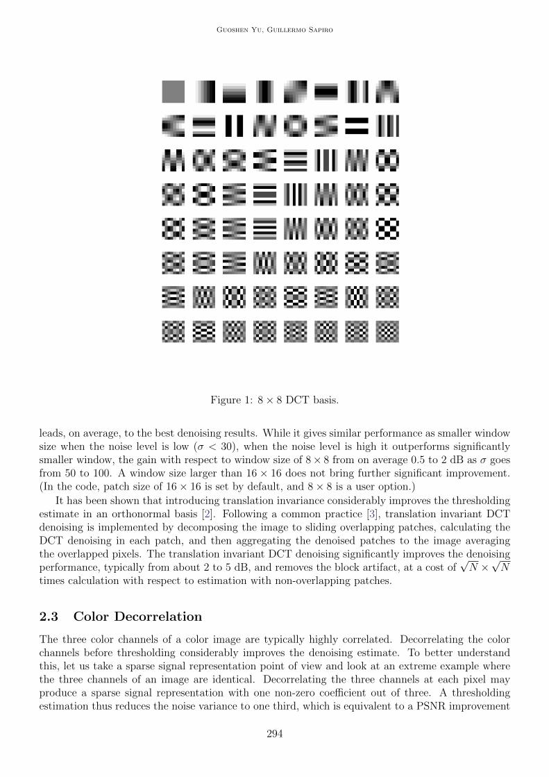
It is well known that local Discrete Cosine Transform (DCT) basis, applied in the most popularimage compression standard JPEG, gives sparse representations of local image patches. Figure 1illustrates an 8× 8 DCT basis.

The proposed denoising algorithm decomposes the image into local patches of size√N = 16×16,

and denoises the patches with thresholding estimate in the DCT domain. The 16× 16 DCT window

293

Guoshen Yu, Guillermo Sapiro

Figure 1: 8× 8 DCT basis.

leads, on average, to the best denoising results. While it gives similar performance as smaller windowsize when the noise level is low (σ < 30), when the noise level is high it outperforms significantlysmaller window, the gain with respect to window size of 8× 8 from on average 0.5 to 2 dB as σ goesfrom 50 to 100. A window size larger than 16 × 16 does not bring further significant improvement.(In the code, patch size of 16× 16 is set by default, and 8× 8 is a user option.)

It has been shown that introducing translation invariance considerably improves the thresholdingestimate in an orthonormal basis [2]. Following a common practice [3], translation invariant DCTdenoising is implemented by decomposing the image to sliding overlapping patches, calculating theDCT denoising in each patch, and then aggregating the denoised patches to the image averagingthe overlapped pixels. The translation invariant DCT denoising significantly improves the denoisingperformance, typically from about 2 to 5 dB, and removes the block artifact, at a cost of

√N ×

√N

times calculation with respect to estimation with non-overlapping patches.

2.3 Color Decorrelation

The three color channels of a color image are typically highly correlated. Decorrelating the colorchannels before thresholding considerably improves the denoising estimate. To better understandthis, let us take a sparse signal representation point of view and look at an extreme example wherethe three channels of an image are identical. Decorrelating the three channels at each pixel mayproduce a sparse signal representation with one non-zero coefficient out of three. A thresholdingestimation thus reduces the noise variance to one third, which is equivalent to a PSNR improvement

294

DCT Image Denoising: a Simple and Effective Image Denoising Algorithm

as high as 10 log10(3) ≈ 4.7dB, orders of magnitude larger than some gain that most denoisingalgorithms struggle to achieve in a single image channel.

An orthonormal basis

{[1/√

3, 1/√

3, 1/√

3]T , [1/√

2, 0, − 1/√

2]T , [1/√

6, − 2/√

6, 1/√

6]T}

is used for color decorrelation. (Note that this is a 3-point DCT basis.) Each decorrelated colorchannel is then denoised separately by the DCT denoising algorithm described above. Comparingwith standard color transformation such as the one from RGB to YUV, the orthonormal colordecomposition slightly improves the denoising performance thanks to its orthogonality. The colordecorrelation typically brings a PSNR improvement from about 1 to 3 dB.

2.4 Computational Complexity

The computational complexity of the DCT image denoising algorithm described above is dominatedby that of the DCT transform of the patches.

A DCT transform of a one-dimensional signal of size N can be implemented with a complexityO(N logN). A two-dimensional DCT transform on an image patch of size

√N ×

√N can be

implemented in a separable way with a complexity O(N log√N) . An image of size S × C, where

S is the number of pixels in each color channel and C , typically equal to 3, is the number of colorchannels, contains S×C sliding patches (slightly less than that in practice due to the border effect).The overall complexity is therefore O(SCN log

√N).

The DCT on different patches can be implemented in parallel, which may significantly reduce thecomputation time.

3 Implementation

The following algorithm (Algorithm 1) is implemented in the C++ source file DCTdenoising.cpp.

Algorithm 1: DCT denoising algorithm.

Input : Noisy image, Gaussian white noise standard deviation σOutput: Denoised imageif image is colored then

decorrelate the color channels of the noisy image (C++ routine: ColorTransform)

Decompose each color channel to sliding patches (C++ routine: Image2Patches)for each image patch do

Calculate 2D-DCT transform of the patch (C++ routine: DCT2D)Threshold the DCT coefficients, with a threshold equal to 3σCalculate inverse 2D-DCT transform of the patch (C++ routine: DCT2D)

Average and aggregate the patches to reconstruct each denoised channel (C++ routine:Patches2Image)

if image is colored thenreverse the color decorrelation to obtain the denoised image from the denoised channels(C++ routine: ColorTransform)

elsethe denoised channel gives the denoised gray-level image

295

Guoshen Yu, Guillermo Sapiro

4 Examples

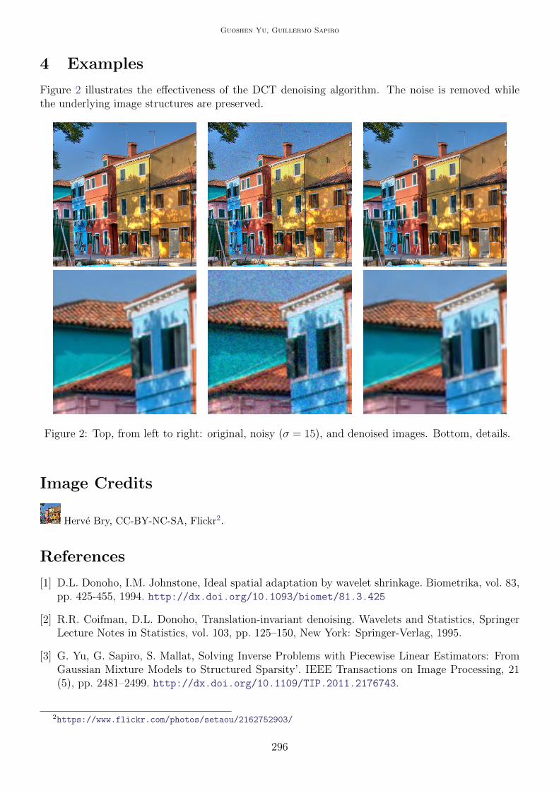
Figure 2 illustrates the effectiveness of the DCT denoising algorithm. The noise is removed whilethe underlying image structures are preserved.

Figure 2: Top, from left to right: original, noisy (σ = 15), and denoised images. Bottom, details.

Image Credits

Herve Bry, CC-BY-NC-SA, Flickr2.

References

[1] D.L. Donoho, I.M. Johnstone, Ideal spatial adaptation by wavelet shrinkage. Biometrika, vol. 83,pp. 425-455, 1994. http://dx.doi.org/10.1093/biomet/81.3.425

[2] R.R. Coifman, D.L. Donoho, Translation-invariant denoising. Wavelets and Statistics, SpringerLecture Notes in Statistics, vol. 103, pp. 125–150, New York: Springer-Verlag, 1995.

[3] G. Yu, G. Sapiro, S. Mallat, Solving Inverse Problems with Piecewise Linear Estimators: FromGaussian Mixture Models to Structured Sparsity’. IEEE Transactions on Image Processing, 21(5), pp. 2481–2499. http://dx.doi.org/10.1109/TIP.2011.2176743.

2https://www.flickr.com/photos/setaou/2162752903/

296