Vol.:(0123456789)1 3

Clim Dyn (2018) 50:2687–2703 DOI 10.1007/s00382-017-3764-0

Decadal-scale teleconnection between South Atlantic SST and southeast Australia surface air temperature in austral summer

Jiaqing Xue1,2 · Jianping Li3,4  · Cheng Sun3 · Sen Zhao5,6 · Jiangyu Mao1 · Di Dong1,2 · Yanjie Li1 · Juan Feng3 

Received: 17 January 2017 / Accepted: 9 June 2017 / Published online: 16 June 2017 © The Author(s) 2017. This article is an open access publication

pathway and spatial scale of the observed SAA wave train are further explained by the Rossby wave ray tracing analysis in non-uniform basic flow. The SAA wave train forced by southwest South Atlantic warming is character-ized by an anomalous anticyclone off the eastern coast of the Australia. Temperature diagnostic analyses based on the thermodynamic equation suggest anomalous northerly flows on western flank of this anticyclone can induce low-level warm advection anomaly over SEA, which thus lead to the warming of surface air temperature there. Finally, SST-forced atmospheric general circulation model ensem-ble experiments also demonstrate that SST forcing in the South Atlantic is associated with the SAA teleconnection wave train in austral summer, this wave train then modulate surface air temperature over SEA on decadal timescales. Hence, observations combined with numerical simulations consistently demonstrate the decadal-scale teleconnection between South Atlantic SST and summertime surface air temperature over SEA.

Keywords South Atlantic decadal variability · South Atlantic–Australia wave train · Southeast Australia · Surface air temperature decadal variability

1 Introduction

Southeast Australia (SEA; south of 30°S and east of 140°E), a highly populated area, is a major center of Aus-tralia’s agriculture, industry and economy. As in many other places of the word, surface air temperature over SEA experienced significant warming during the twentieth cen-tury (Stocker et  al. 2014). Accompanied by accelerated warming over SEA since the 1950s (Murphy and Timbal 2008; Ashcroft et  al. 2012; Fierro and Leslie 2014), high

Abstract Austral summer (December–February) sur-face air temperature over southeast Australia (SEA) is found to be remotely influenced by sea surface tempera-ture (SST) in the South Atlantic at decadal time scales. In austral summer, warm SST anomalies in the southwest South Atlantic induce concurrent above-normal surface air temperature over SEA. This decadal-scale teleconnec-tion occurs through the eastward propagating South Atlan-tic–Australia (SAA) wave train triggered by SST anoma-lies in the southwest South Atlantic. The excitation of the SAA wave train is verified by forcing experiments based on both linear barotropic and baroclinic models, propagation

* Jianping Li ljp@bnu.edu.cn

* Cheng Sun scheng@bnu.edu.cn

1 State Key Laboratory of Numerical Modeling for Atmospheric Sciences and Geophysical Fluid Dynamics, Institute of Atmospheric Physics, Chinese Academy of Sciences, Beijing 100029, China

2 College of Earth Science, University of Chinese Academy of Sciences, Beijing 100049, China

3 State Key Laboratory of Earth Surface Processes and Resource Ecology and College of Global Change and Earth System Science, Beijing Normal University, Beijing 100875, China

4 Laboratory for Regional Oceanography and Numerical Modeling, Qingdao National Laboratory for Marine Science and Technology, Qingdao 266237, China

5 Key Laboratory of Meteorological Disaster of Ministry of Education, and College of Atmospheric Science, Nanjing University of Information Science and Technology, Nanjing 210044, China

6 Department of Atmospheric Sciences, University of Hawai‘i at Mānoa, Honolulu, HI 96822, USA

2688 J. Xue et al.

1 3

temperature extremes are becoming more and more fre-quent over SEA (Alexander et al. 2006; Perkins et al. 2012; Lewis and Karoly 2013; Morak et  al. 2013), posing an increasing threat to human health and property (Hansen et  al. 2008; Karoly 2009). The accelerated warming over SEA since the 1950s may be caused by a combination of large-scale anthropogenic warming and natural decadal variability at regional scale. As such, investigation of the drivers and processes responsible for surface air tempera-ture decadal variability over SEA is very important.

Many previous studies have linked Australian climate to various large-scale remote climate drivers (Risbey et al. 2009; Ummenhofer et al. 2011; Hunter and Binyamin 2012; Fierro and Leslie 2014), and most of these studies focused on rainfall variability. The El Niño–Southern Oscillation (ENSO) (Taschetto and England 2009; Cai et  al. 2011; Ummenhofer et  al. 2011), Indian Ocean Dipole (IOD) (Risbey et al. 2009; Cai et al. 2011), Southern Hemisphere annular mode (SAM) (Hendon et  al. 2007; Meneghini et al. 2007; Risbey et al. 2009; Feng et al. 2010a), sea sur-face temperature (SST) in the Wharton Basin (Li et  al. 2012a) and monsoon-like Southwest Australian circulation (SWAC) (Feng et  al. 2010b, 2015; Li et  al. 2011) are all reported to modulate Australian rainfall on interannual time scales. On decadal time scales, positive (negative) phases of the Interdecadal Pacific Oscillation (IPO) can induce reduced (increased) rainfall in eastern Australia (Verdon et  al. 2004; Dong and Dai 2015). Moreover, the North Atlantic Oscillation (NAO) was also shown to be able to influence subtropical eastern Australia rainfall through the delayed adjustment of the Atlantic meridional overturning circulation (AMOC) (Sun et al. 2015a).

As for Australian surface air temperature variability, the mean surface air temperature and maximum surface air temperature over Australia are shown to be connected to ENSO on interannual timescales. El Niño events are associ-ated with increased surface air temperature, while La Niña events commonly induce decreased air temperature (Power et al. 1998, 1999; Jones and Trewin 2000; Fierro and Leslie 2014). However, the air temperature–ENSO relationship is unstable, with a weak relation during IPO positive phases, but a stronger relation when the IPO cools the tropical Pacific Ocean (Power et al. 1999; Ashcroft et al. 2012). The out-of-phase variation between the SAM index and surface air temperature over SEA was also noted in some previ-ous studies (Gillett et  al. 2006; Hendon et  al. 2007; Wat-terson 2009). On decadal time scales, Dong and Dai (2015) documented a positive correlation between the IPO index and annual-mean surface air temperature over central and northern Australia, and this relationship is further found to be strongest in austral summer. However, the IPO can-not explain the decadal change of surface air temperature over SEA, thus the possible climate drivers for surface air

temperature decadal change over SEA remain unclear. Our preliminary analysis finds summertime surface air temper-ature decadal variation over SEA has a close relationship with South Atlantic SST, which may therefore be a plausi-ble driver.

The South Atlantic plays a unique role in global energy balance by transporting energy towards the equator as a part of global conveyor (Gordon 1986). The South Atlan-tic decadal variability has received less attention compared with the well observed North Atlantic historically, however there has been an increasing effort of the climate research community to elucidate South Atlantic decadal variability and corresponding climate impacts in recent years (Sterl and Hazeleger 2003; Haarsma et  al. 2005; Lopez et  al. 2016a, b; Nnamchi et  al. 2016). Based on the empirical orthogonal function (EOF) analysis of global SST anoma-lies, several studies have identified a decadal-scale inter-hemispheric SST dipole mode, which is mainly character-ized by SST anomalies of opposing sign between the North and South Atlantic (Parker et  al. 2007; Dima and Lohm-ann 2010; Sun et al. 2013). This decadal-scale dipole mode was shown to be associated with the fluctuation of AMOC (Vellinga and Wood 2002; Wang et  al. 2014; Sun et  al. 2015b; Lopez et al. 2016b), and can be used to indicate the strength of the AMOC (Latif et al. 2006). Some other stud-ies highlighted the role of local air–sea coupling confined to the South Atlantic in the decadal variability of the South Atlantic (Venegas et  al. 1997; Wainer and Venegas 2002; Nnamchi et  al. 2016). In addition, IPO forcing was also documented to be able to cause SST decadal change in the South Atlantic through the teleconnection wave train ema-nating from tropical Pacific to the South Atlantic. Though various mechanisms have been proposed to explain the decadal variability of the South Atlantic in previous stud-ies, few attention has been paid to explore the possible cli-mate impacts of the South Atlantic on decadal timescales (Wainer and Soares 1997; Robertson et  al. 2003; Lopez et al. 2016b). Recent study found anomalous South Atlantic meridional heat transport can cause lagged SST anomalies in the South Atlantic due to convergence/divergence of heat on decadal timescales, these SST anomalies can then force anomalous Hadley circulation and modulate the strength of monsoon (Lopez et al. 2016b). Overall, our understanding of the decadal climate impacts of the South Atlantic is still very limited, further investigation into this topic is needed.

This study will focus on the decadal-scale teleconnec-tion between South Atlantic SST and austral summer sur-face air temperature over SEA, as well as the underlying mechanism for this teleconnection. The remainder of this paper is organized as follows. Datasets and methods used in this study are described in Sect.  2. Section 3 reveals a decadal-scale covariability between South Atlantic SST and summertime surface air temperature over Australia.

2689Decadal-scale teleconnection between South Atlantic SST and southeast Australia surface…

1 3

Section  4 provides possible physical explanations for this decadal-scale teleconnection. SST-forced atmospheric gen-eral circulation model (AGCM) ensemble simulations are further utilized in Sect. 5 to verify the existence of the dec-adal-scale teleconnection. Section  6 contains a summary and discussion.

2 Datasets and methods

2.1 Datasets

Gridded monthly mean land surface air temperature used in this study is UDEL dataset version 4.01, which is obtained from the University of Delaware spanning the period 1900–2010 on a 0.5°  ×  0.5° grid (Legates and Willmott 1990). The relatively high resolution of this dataset makes it particularly suitable for climate research at regional scale. Rainfall for the Australian continent is provided by the Bureau of Meteorology (BoM) on a 0.25° × 0.25° grid for the period 1900–2010 (Jones et al. 2009).

The gridded SST dataset is the monthly extended recon-structed sea surface temperature version 4 (ERSSTv4), which adopts new bias adjustments, quality control proce-dures and analysis methods compared to the older version 3b (Huang et al. 2015). It covers the period from 1854 to the present on a 2°  ×  2° latitude–longitude grid. In addi-tion, HadISST version 2.1 (obtained as the 10-member ensemble mean from European Center for Medium-Range Weather Forecasts (ECMWF) atmospheric model integra-tions (ERA-20CM)) is also used to examine the reliability of the results (Rayner et al. 2013, in preparation; Hersbach et  al. 2015). Atmospheric reanalysis data including wind, geopotential height and air temperature are taken from the ECMWF atmospheric reanalysis of the twentieth century (ERA-20C) (Poli et al. 2016). This reanalysis dataset cov-ers a period of 1900–2010 with horizontal resolution of approximately 125 km and vertical coverage from 1000 to 1 hPa. The ERA-20C reanalysis is produced using the Inte-grated Forecasting System (IFS) model in a 4-D Var sys-tem to assimilate surface pressure as well as ocean surface wind with sea-ice and SST from HadISST2.1 as boundary forcing.

Atmosphere-only model simulations used in this study are derived from the ERA-20CM dataset, which is an

Atmospheric Model Intercomparison Project (AMIP)-style experiment including an ensemble of 10 IFS atmospheric simulations integrated by the ECMWF, covering the period 1899–2010 (Hersbach et al. 2015). The IFS model adopts T159 spectral resolution in the horizontal and includes 91 vertical levels. The ten simulations are generated using ten realizations of slightly different boundary HadISST2.1 and sea-ice cover to overcome uncertainties in observational sources. All ten ensemble members use exactly the same radiative forcing suggested by the fifth phase of the Cou-pled Model Intercomparison Project (CMIP5). The results derived from ERA-20CM will be referred to as the AMIP-style ensemble in the remainder of this paper.

Due to relatively large uncertainties in surface observa-tions before 1900, all the analyses in the present study are restricted to the period 1900–2010. Because our particular interest is in the climate impacts of the South Atlantic on decadal time scales, all the variables are linearly detrended first, and then processed with an 11-year running mean to highlight decadal signals. Summer in this study refers to the austral season and is defined as December, January and February (DJF). Anomalies are obtained with respect to the 1900–2000 climatology.

2.2 Statistical methods

The tests of statistical significance for linear correlation and regression between two auto-correlated time series are based on Student’s t test using an effective number of degrees of freedom Neff derived from the following approximation:

where N represents the sample size, and �XX(j) and �YY (j) denote the autocorrelations of time series X and Y at time lag j, respectively (Li et al. 2012b, 2013).

2.3 Wave activity flux

A phase-independent wave activity flux formulated by Takaya and Nakamura (2001) is used to diagnose the prop-agation of stationary Rossby wave. The horizoantal compo-nent of the wave activity flux can be expressed as follows:

(1)1

Neff≈

1

N+

2

N

N∑j=1

N − j

N�XX(j)�YY (j),

(2)W =p cos�

2�U�

⎛⎜⎜⎜⎜⎜⎝

u

a2cos2�

���� �

��

�2

− � � �2� �

��2

�+

v

a2 cos�

��� �

��

�� �

��− � � �

2� �

����

�

u

a2 cos�

��� �

��

�� �

��− � � �

2� �

����

�+

v

a2

���� �

��

�2

− � � �2� �

��2

�

⎞⎟⎟⎟⎟⎟⎠

,

2690 J. Xue et al.

1 3

where � ′ is perturbation geostrophic streamfunction, U = (u, v) denotes horizontal basic flow, p is pressure nor-malized by 1000 hPa.

2.4 Theoretical models

The linear barotropic model in a steady state can be expressed in the form of the vorticity equation:

where J denotes a Jacobian operator, �̄� and � ′ stand for basic state and perturbation streamfunctions, f represents the Coriolis parameter and S′ is the anomalous vorticity forcing associated with divergent wind. The biharmonic diffusion coefficient v is set to a damping time scale of l day for the smallest wave while the Rayleigh friction coefficient � has a damping time scale of 10 days. The model is solved using a spherical harmonic expansion with T42 truncation (Watanabe 2004).

The linear baroclinic model (LBM) employed in this study is constructed by linearizing the primitive equa-tions about a 3D climatological basic state. This model has a T42 horizontal spectral resolution and 20 vertical levels on a sigma coordinate with vorticity, divergence, temperature and the logarithm of surface pressure as model variables. Details of the model formulation can be found in Watanabe and Kimoto (2000). Horizontal and vertical diffusion, Newtonian damping and Rayleigh friction are all included in the model. The biharmonic horizontal diffusion is set with a damping time scale of

(3)J(�̄� ,∇2𝜓 �) + J(𝜓 �,∇2�̄� + f ) + 𝜈∇6𝜓 � + 𝛼∇2𝜓 � = S�,

1 day for the smallest wave. Weak vertical diffusion with a damping time scale of 1000  days is adopted to sup-press vertical computational noise. Newtonian damping and Rayleigh friction represented as linear drag have a time scale of 0.2  days in the lower boundary layer and 30  days at mid-levels. With the above dissipation set-tings, the model takes about 25 days to achieve a steady state. As such, the average for days 31–35 is presented as the steady response.

2.5 Thermodynamic equation

The thermodynamic equation is used for diagnostic analy-sis of the air temperature over SEA, and is briefly intro-duced as follows:

where T is temperature, u and v represent zonal and meridi-onal wind respectively, and � is the vertical velocity in pressure coordinates. Sp is the static stability parameter specified as Sp =

RT

cpp−

�T

�p, where R is the gas constant for

dry air and cp is the specific heat at constant pressure. Here also J is the rate of heating per unit mass due to diabatic processes. The terms on the right-hand side of the thermo-dynamic equation, from left to right, characterize zonal advection, meridional advection, adiabatic heating and dia-batic heating.

(4)�T

�t= −u

�T

�x− v

�T

�y+ Sp� +

J

cp,

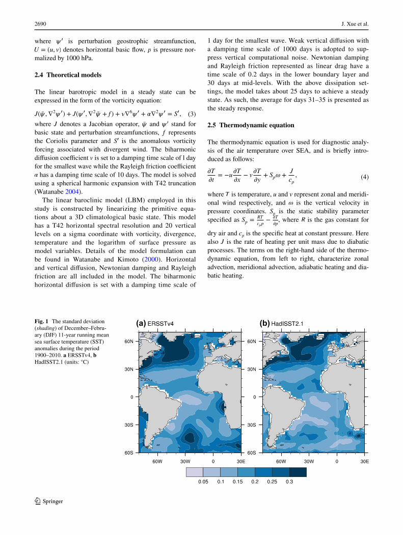
Fig. 1 The standard deviation (shading) of December–Febru-ary (DJF) 11-year running mean sea surface temperature (SST) anomalies during the period 1900–2010. a ERSSTv4, b HadISST2.1 (units: °C)

(a) (b)

2691Decadal-scale teleconnection between South Atlantic SST and southeast Australia surface…

1 3

3 Decadal-scale covariability between South Atlantic SST and surface air temperature over Australia in austral summer

Figure 1a shows the standard deviation of DJF 11-year run-ning mean SST anomalies based on dataset ERSSTv4 to measure the strength of Atlantic decadal variability, there are several areas stand out as having noticeable SST vari-ability at decadal time scales. The most prominent area in this map is the North Atlantic, which manifests the SST variability connected to the Atlantic Multidecadal Variabil-ity (AMV). In addition to the North Atlantic, the standard deviation map also indicates remarkable SST decadal vari-ability in southwest South Atlantic, primarily confined to the domain 25°–50°S, 50°–10°W, where the magnitude of decadal SST variability is comparable to that in the North Atlantic. The standard deviation map calculated from another dataset HadISST2.1 (Fig.  1b) exhibits almost the same pattern as that in Fig. 1a, also with a notable center in the southwest South Atlantic. Two independent sets of SST data consistently indicate prominent decadal change in the southwest South Atlantic, thus similar to the North Atlan-tic, the strong decadal variability in South Atlantic may also have widespread climate impacts.

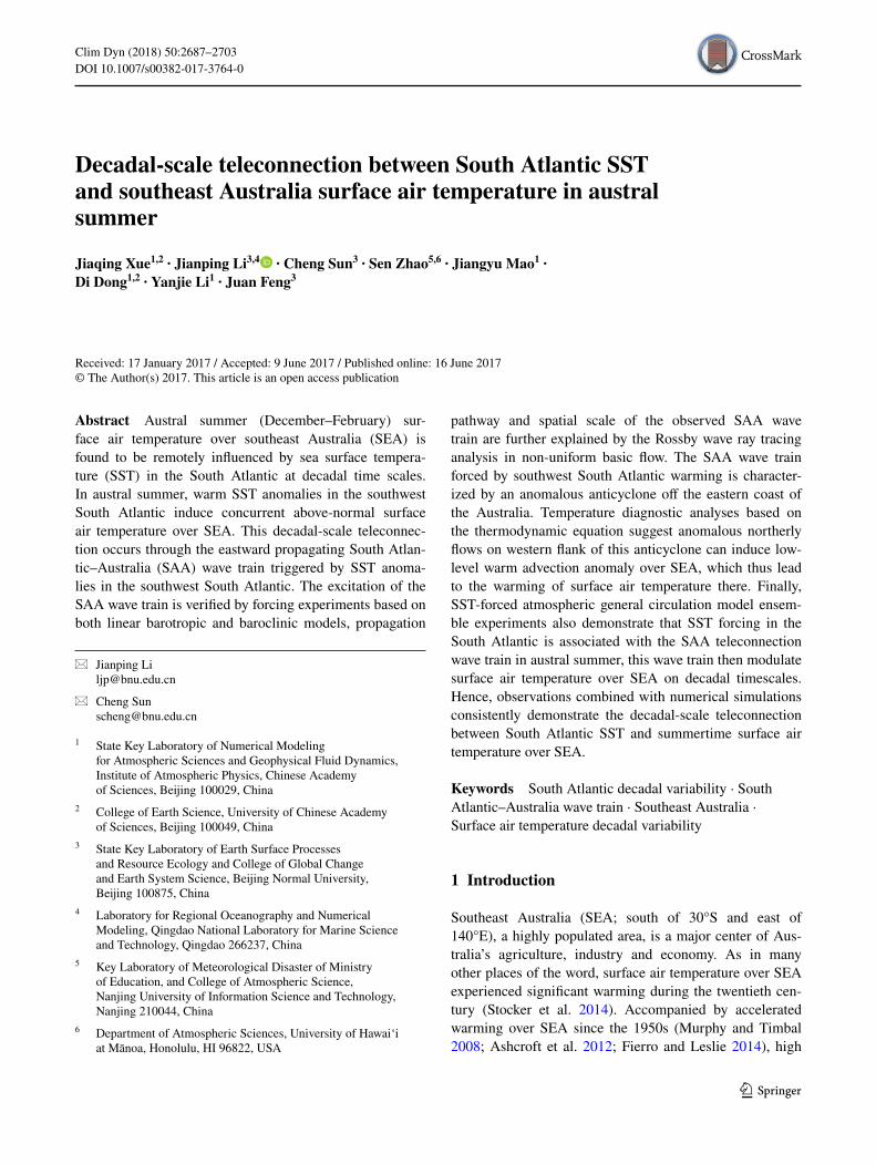
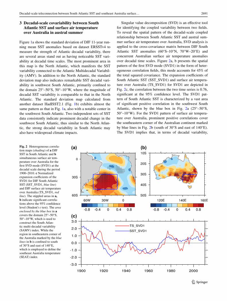
Singular value decomposition (SVD) is an effective tool for identifying the coupled variability between two fields. To reveal the spatial pattern of the decadal-scale coupled relationship between South Atlantic SST and austral sum-mer surface air temperature over Australia, SVD analysis is applied to the cross-covariance matrix between DJF South Atlantic SST anomalies (60°S–10°N, 70°W–20°E) and concurrent Australian surface air temperature anomalies over decadal time scales. Figure 2a, b presents the spatial pattern of the first SVD mode (SVD1) in the form of heter-ogeneous correlation fields, this mode accounts for 45% of the total squared covariance. The expansion coefficients of South Atlantic SST (SST_SVD1) and surface air tempera-ture over Australia (TS_SVD1) for SVD1 are depicted in Fig. 2c, the correlation between the two time series is 0.76, significant at the 95% confidence level. The SVD1 pat-tern of South Atlantic SST is characterized by a vast area of significant positive correlation in the southwest South Atlantic, shown by the blue box in Fig.  2a (25°–50°S, 50°–10°W). For the SVD1 pattern of surface air tempera-ture over Australia, prominent positive correlations cover the southeastern corner of the Australian continent marked by blue lines in Fig. 2b (south of 30°S and east of 140°E). The SVD1 implies that, in terms of decadal variability,

Fig. 2 Heterogeneous correla-tion maps (shading) of a DJF SST in South Atlantic and b simultaneous surface air tem-perature over Australia for the first SVD mode (SVD1) at the decadal scale during the period 1900–2010. c Normalized expansion coefficients of the SVD1 for DJF South Atlantic SST (SST_SVD1, blue line) and DJF surface air temperature over Australia (TS_SVD1, red line). The stippled areas in a, b indicate significant correla-tions above the 95% confidence level (Student’s t test). The area enclosed by the blue box in a covers the domain 25°–50°S, 50°–10°W, which is used to construct the South Atlan-tic multi-decadal variability (SAMV) index. While the region in southeastern corner of the Australia marked by the blue lines in b is confined to south of 30°S and east of 140°E, which is employed to define the southeast Australia temperature (SEAT) index

(a) (b)

(c)

2692 J. Xue et al.

1 3

when SST is above normal in the southwest South Atlantic, SEA tends to experience a warmer climate during the aus-tral summer season.

Based on the key areas identified in SVD analysis, we constructed the South Atlantic multidecadal variability (SAMV) index, which is defined as the domain-averaged DJF SST anomalies over the region 25°–50°S, 50°–10°W in the South Atlantic (blue box in Fig.  2a). Latif et  al. (2006) used a box in southwest South Atlantic (40°–60°S, 50°W–0°) to measure the multidecadal variability of the South Atlantic. However, standard deviation of SST shown in Fig.  1 displays the strongest decadal change over the region (25°–50°S, 50°–10°W), which is a little bit north to the box used in Latif et al. (2006). Thus, to better char-acterize the decadal change in South Atlantic, we define the SAMV index over the region (25°–50°S, 50°–10°W) in southwest South Atlantic, similar to the location of south-west pole of the interannual South Atlantic Ocean dipole (SAOD) (Morioka et  al. 2011; Nnamchi et  al. 2011). Because the SAMV indices defined based on datasets

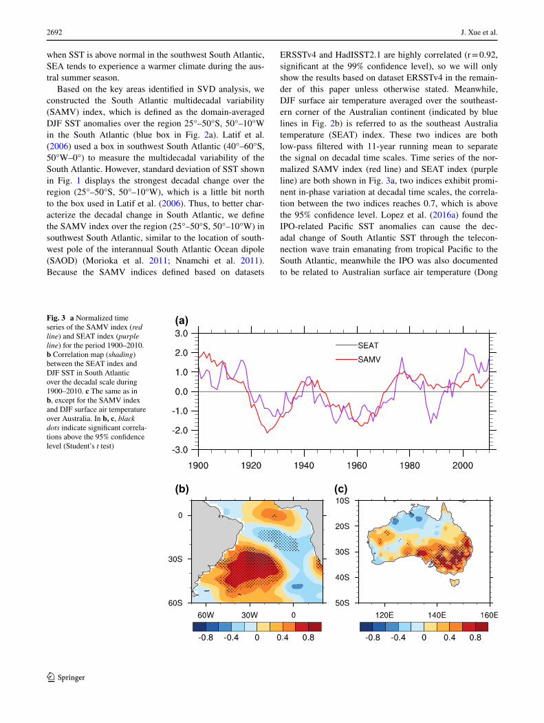
ERSSTv4 and HadISST2.1 are highly correlated (r = 0.92, significant at the 99% confidence level), so we will only show the results based on dataset ERSSTv4 in the remain-der of this paper unless otherwise stated. Meanwhile, DJF surface air temperature averaged over the southeast-ern corner of the Australian continent (indicated by blue lines in Fig.  2b) is referred to as the southeast Australia temperature (SEAT) index. These two indices are both low-pass filtered with 11-year running mean to separate the signal on decadal time scales. Time series of the nor-malized SAMV index (red line) and SEAT index (purple line) are both shown in Fig. 3a, two indices exhibit promi-nent in-phase variation at decadal time scales, the correla-tion between the two indices reaches 0.7, which is above the 95% confidence level. Lopez et  al. (2016a) found the IPO-related Pacific SST anomalies can cause the dec-adal change of South Atlantic SST through the telecon-nection wave train emanating from tropical Pacific to the South Atlantic, meanwhile the IPO was also documented to be related to Australian surface air temperature (Dong

Fig. 3 a Normalized time series of the SAMV index (red line) and SEAT index (purple line) for the period 1900–2010. b Correlation map (shading) between the SEAT index and DJF SST in South Atlantic over the decadal scale during 1900–2010. c The same as in b, except for the SAMV index and DJF surface air temperature over Australia. In b, c, black dots indicate significant correla-tions above the 95% confidence level (Student’s t test)

(a)

(b) (c)

2693Decadal-scale teleconnection between South Atlantic SST and southeast Australia surface…

1 3

and Dai 2015). To investigate whether the decadal-scale covariability between South Atlantic SST and summertime surface air temperature over SEA is independent of IPO, we further calculate the correlation between SAMV index and SEAT index with the IPO signal linearly removed. After removing IPO, the correlation coefficient reaches 0.6, which is still significant at the 95% confidence level, this means the decadal-scale covariability is independent of IPO.

Cross-correlation analyses are further conducted to ascertain the covariability between southwest South Atlan-tic SST and summertime surface air temperature over SEA. Figure  3b gives the correlation map between the SEAT index and DJF SST anomalies in the South Atlan-tic at decadal time scales, this pattern projects strongly onto Fig.  2a with significant positive correlation in the southwest South Atlantic. In addition, the correlation field between the SAMV index and DJF surface air tem-perature over Australia shown in Fig. 3c also agrees well with Fig.  2b, both with significant positive correlation over SEA. By comparing Fig.  3b, c with Fig.  2a, b, it is found that the decadal-scale coupled mode between South Atlantic SST and surface air temperature over SEA identi-fied by SVD analysis can be closely reproduced by sim-ple cross-correlations with defined indices, which further demonstrates this decadal-scale covariability is dominant and robust.

4 Possible mechanism for the decadal-scale teleconnection

4.1 Teleconnection wave train bridging the South Atlantic and SEA

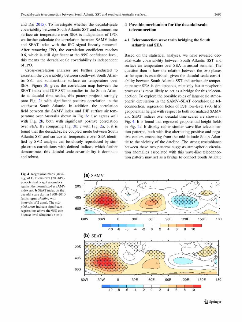
Based on the statistical analyses, we have revealed dec-adal-scale covariability between South Atlantic SST and surface air temperature over SEA in austral summer. The question then is how the relation between the two places so far apart is established, given the decadal-scale covari-ability between South Atlantic SST and surface air temper-ature over SEA is simultaneous, relatively fast atmospheric processes is most likely to act as a bridge for this telecon-nection. To explore the possible roles of large-scale atmos-pheric circulation in the SAMV–SEAT decadal-scale tel-econnection, regression fields of DJF low-level (700  hPa) geopotential height with respect to both normalized SAMV and SEAT indices over decadal time scales are shown in Fig. 4. It is found that regressed geopotential height fields in Fig.  4a, b display rather similar wave-like teleconnec-tion patterns, both with five alternating positive and nega-tive centers emanating from the mid-latitude South Atlan-tic to the vicinity of the dateline. The strong resemblance between these two patterns suggests atmospheric circula-tion anomalies associated with this wave-like teleconnec-tion pattern may act as a bridge to connect South Atlantic

Fig. 4 Regression maps (shad-ing) of DJF low-level (700 hPa) geopotential height anomalies against the normalized a SAMV index and b SEAT index on the decadal scale during 1900–2010 (units: gpm, shading with intervals of 2 gpm). The stip-pled areas indicate significant regressions above the 95% con-fidence level (Student’s t test)

(a)

(b)

2694 J. Xue et al.

1 3

SST anomalies and downstream climate variability in Australia.

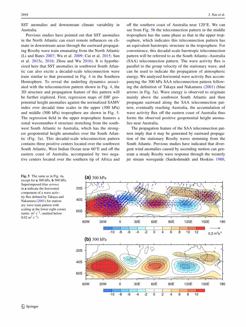
Previous studies have pointed out that SST anomalies in the North Atlantic can exert remote influences on cli-mate in downstream areas through the eastward propagat-ing Rossby wave train emanating from the North Atlantic (Li and Bates 2007; Wu et al. 2009; Cui et al. 2015; Sun et  al. 2015c, 2016; Zhou and Wu 2016). It is hypothe-sized here that SST anomalies in southwest South Atlan-tic can also excite a decadal-scale teleconnection wave train similar to that presented in Fig.  4 in the Southern Hemisphere. To reveal the underling dynamics associ-ated with the teleconnection pattern shown in Fig. 4, the 3D structure and propagation feature of this pattern will be further explored. First, regression maps of DJF geo-potential height anomalies against the normalized SAMV index over decadal time scales in the upper (300  hPa) and middle (500  hPa) troposphere are shown in Fig.  5. The regression field in the upper troposphere features a zonal wavenumber-4 structure stretching from the south-west South Atlantic to Australia, which has the strong-est geopotential height anomalies over the South Atlan-tic (Fig.  5a). This decadal-scale teleconnection pattern contains three positive centers located over the southwest South Atlantic, West Indian Ocean near 60°E and off the eastern coast of Australia, accompanied by two nega-tive centers located over the southern tip of Africa and

off the southern coast of Australia near 120°E. We can see from Fig. 5b the teleconnection pattern in the middle troposphere has the same phase as that in the upper trop-osphere, which indicates this teleconnection pattern has an equivalent barotropic structure in the troposphere. For convenience, this decadal-scale barotropic teleconnection pattern will be referred to as the South Atlantic–Australia (SAA) teleconnection pattern. The wave activity flux is parallel to the group velocity of the stationary wave, and can be used to indicate the propagation of atmospheric energy. We analyzed horizontal wave activity flux accom-panying the 300 hPa SAA teleconnection pattern follow-ing the definition of Takaya and Nakamura (2001) (blue arrows in Fig. 5a). Wave energy is observed to originate mainly above the southwest South Atlantic and then propagate eastward along the SAA teleconnection pat-tern, eventually reaching Australia, the accumulation of wave activity flux off the eastern coast of Australia thus forms the observed positive geopotential height anoma-lies near Australia.

The propagation feature of the SAA teleconnection pat-tern imply that it may be generated by eastward propaga-tion of the stationary Rossby waves stemming from the South Atlantic. Previous studies have indicated that diver-gent wind anomalies caused by ascending motion can gen-erate a steady Rossby wave response through the westerly jet stream waveguide (Sardeshmukh and Hoskins 1988;

Fig. 5 The same as in Fig. 4a, except for a 300 hPa, b 500 hPa. Superimposed blue arrows in a indicate the horizontal component of a wave activ-ity flux defined by Takaya and Nakamura (2001) for station-ary wave train pattern with scaling at the lower right corner (units: m2 s−2, omitted below 0.02 m2 s−2)

(a)

(b)

2695Decadal-scale teleconnection between South Atlantic SST and southeast Australia surface…

1 3

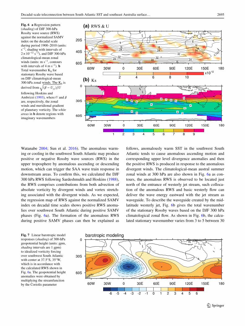
Watanabe 2004; Sun et  al. 2016). The anomalous warm-ing or cooling in the southwest South Atlantic may produce positive or negative Rossby wave sources (RWS) in the upper troposphere by anomalous ascending or descending motion, which can trigger the SAA wave train response in downstream areas. To confirm this, we calculated the DJF 300 hPa RWS following Sardeshmukh and Hoskins (1988), the RWS comprises contributions from both advection of absolute vorticity by divergent winds and vortex stretch-ing associated with the divergent winds. As we expected, the regression map of RWS against the normalized SAMV index on decadal time scales shows positive RWS anoma-lies over southwest South Atlantic during positive SAMV phases (Fig.  6a). The formation of the anomalous RWS during positive SAMV phases can then be explained as

follows, anomalously warm SST in the southwest South Atlantic tends to cause anomalous ascending motion and corresponding upper level divergence anomalies and then the positive RWS is produced in response to the anomalous divergent winds. The climatological-mean austral summer zonal winds at 300 hPa are also shown in Fig. 6a as con-tours, the anomalous RWS is observed to be located just north of the entrance of westerly jet stream, such colloca-tion of the anomalous RWS and basic westerly flow can deliver the wave energy eastward with the jet stream as waveguide. To describe the waveguide created by the mid-latitude westerly jet, Fig.  6b gives the total wavenumber of the stationary Rossby waves based on the DJF 300 hPa climatological zonal flow. As shown in Fig. 6b, the calcu-lated stationary wavenumber varies from 3 to 5 between 30

Fig. 6 a Regression pattern (shading) of DJF 300-hPa Rossby wave source (RWS) against the normalized SAMV index on the decadal scale during period 1900–2010 (units: s−2, shading with intervals of 2 × 10−12 s−2), and DJF 300-hPa climatological-mean zonal winds (units: m s−1, contours with intervals of 4 m s−1). b Total wavenumber KS for stationary Rossby wave based on DJF climatological-mean 300-hPa zonal winds. The KS is derived from

√(� − Uyy)∕U

following Hoskins and Ambrizzi (1993), where U and � are, respectively, the zonal winds and meridional gradient of planetary vorticity. The white areas in b denote regions with imaginary wavenumbers

(a)

(b)

Fig. 7 Linear barotropic model responses (shading) of 300-hPa geopotential height (units: gpm, shading intervals are 1 gpm) to idealized vorticity forcing over southwest South Atlantic with center at 37.5°S, 35°W, which is in accordance with the calculated RWS shown in Fig. 6a. The geopotential height anomalies were obtained by multiplying the streamfunction by the Coriolis parameter

2696 J. Xue et al.

1 3

and 60°S, which is in agreement with the observed zonal wavenumber-4 structure of the SAA teleconnection pattern. Therefore, the mechanism for the observed SAA telecon-nection pattern may be attributed to the stationary Rossby wave train response to the anomalous RWS caused by SAMV.

To check whether the anomalous RWS forcing over the South Atlantic can induce the observed SAA teleconnec-tion pattern, an idealized RWS over the South Atlantic similar to that shown in Fig.  6a is used to force a linear barotropic model with climatological DJF 300 hPa stream function as background field. The steady response of the geopotential height field to this anomalous RWS is depicted in Fig.  7, which features a clear wave train pattern origi-nating from the South Atlantic to Australia with alternate positive and negative centers. This five-center wave train response comprises three positive centers and two negative centers in between, broadly consistent with the distribution of the SAA teleconnection pattern, signifying that Rossby wave dynamics captures the essential mechanism responsi-ble for the SAA teleconnection pattern.

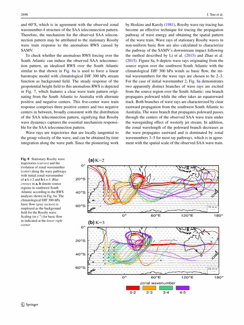
Wave rays are trajectories that are locally tangential to the group velocity of the wave, and can be obtained by time integration along the wave path. Since the pioneering work

by Hoskins and Karoly (1981), Rossby wave ray tracing has become an effective technique for tracing the propagation pathway of wave energy and obtaining the spatial pattern of the wave train. Wave rays of stationary Rossby waves in non-uniform basic flow are also calculated to characterize the pathway of the SAMV’s downstream impact following the method described by Li et  al. (2015) and Zhao et  al. (2015). Figure 8a, b depicts wave rays originating from the source region over the southwest South Atlantic with the climatological DJF 300  hPa winds as basic flow, the ini-tial wavenumbers for the wave rays are chosen to be 2–3. For the case of initial wavenumber 2, Fig. 8a demonstrates two apparently distinct branches of wave rays are excited from the source region over the South Atlantic: one branch propagates poleward while the other takes an equatorward track. Both branches of wave rays are characterized by clear eastward propagation from the southwest South Atlantic to Australia. The wave branch that propagates poleward passes through the centers of the observed SAA wave train under the waveguiding effect of westerly jet stream. In addition, the zonal wavelength of the poleward branch decreases as the wave propagates eastward and is dominated by zonal wavenumbers 3–5 for most ray pathways, which is in agree-ment with the spatial scale of the observed SAA wave train.

Fig. 8 Stationary Rossby wave trajectories (curves) and the evolution of zonal wavenumber (color) along the wave pathways with initial zonal wavenumber of a k = 2 and b k = 3. Blue crosses in a, b denote source regions in southwest South Atlantic according to the RWS analyses shown in Fig. 6a. The climatological DJF 300-hPa basic flow (gray vectors) is employed as the background field for the Rossby wave. Scaling (m s−1) for basic flow in indicated at the lower right corner

(a)

(b)

2697Decadal-scale teleconnection between South Atlantic SST and southeast Australia surface…

1 3

For the wavenumber-3 scenario in Fig. 8b, most wave rays are trapped over the southern tip of the African continent, and only a few of them can extend eastward to the Aus-tralia. Therefore, the wavenumber-2 scenario dominates the eastward transport of wave energy from the source region over the South Atlantic to Australia. These results of the wave ray tracing analysis help to further explain the path-way and spatial scale of the observed SAA wave train.

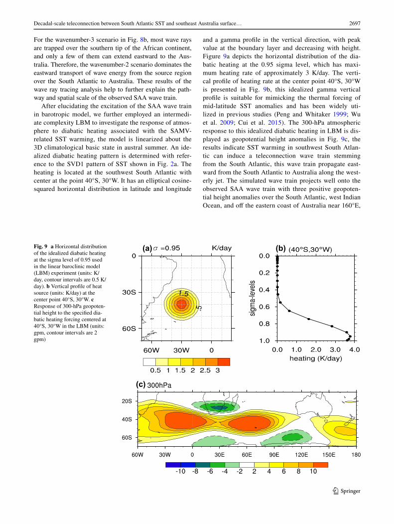
After elucidating the excitation of the SAA wave train in barotropic model, we further employed an intermedi-ate complexity LBM to investigate the response of atmos-phere to diabatic heating associated with the SAMV-related SST warming, the model is linearized about the 3D climatological basic state in austral summer. An ide-alized diabatic heating pattern is determined with refer-ence to the SVD1 pattern of SST shown in Fig. 2a. The heating is located at the southwest South Atlantic with center at the point 40°S, 30°W. It has an elliptical cosine-squared horizontal distribution in latitude and longitude

and a gamma profile in the vertical direction, with peak value at the boundary layer and decreasing with height. Figure  9a depicts the horizontal distribution of the dia-batic heating at the 0.95 sigma level, which has maxi-mum heating rate of approximately 3  K/day. The verti-cal profile of heating rate at the center point 40°S, 30°W is presented in Fig.  9b, this idealized gamma vertical profile is suitable for mimicking the thermal forcing of mid-latitude SST anomalies and has been widely uti-lized in previous studies (Peng and Whitaker 1999; Wu et  al. 2009; Cui et  al. 2015). The 300-hPa atmospheric response to this idealized diabatic heating in LBM is dis-played as geopotential height anomalies in Fig.  9c, the results indicate SST warming in southwest South Atlan-tic can induce a teleconnection wave train stemming from the South Atlantic, this wave train propagate east-ward from the South Atlantic to Australia along the west-erly jet. The simulated wave train projects well onto the observed SAA wave train with three positive geopoten-tial height anomalies over the South Atlantic, west Indian Ocean, and off the eastern coast of Australia near 160°E,

Fig. 9 a Horizontal distribution of the idealized diabatic heating at the sigma level of 0.95 used in the linear baroclinic model (LBM) experiment (units: K/day, contour intervals are 0.5 K/day). b Vertical profile of heat source (units: K/day) at the center point 40°S, 30°W. c Response of 300-hPa geopoten-tial height to the specified dia-batic heating forcing centered at 40°S, 30°W in the LBM (units: gpm, contour intervals are 2 gpm)

(a) (b)

(c)

2698 J. Xue et al.

1 3

and two negative centers located over the southern tip of Africa and off the southern coast of Australia at longi-tude 110°E. We can see the geopotential height anoma-lies near the Australia in LBM is farther to the south compared with the observation, however this bias does not appear in the AGCM experiments, which will be dis-cussed in Sect.  5. Different from AGCM, complex non-linear interactions cannot be described by LBM, which may be the cause of this southward shift of geopotential height anomalies near Australia.

The above forcing experiments with SAMV-related vorticity forcing in barotropic model and diabatic heating forcing in LBM consistently demonstrate the fundamen-tal roles of the southwest South Atlantic SST anomalies in the generation of the observed decadal-scale SAA tel-econnection wave train.

4.2 Temperature diagnostic analysis over Australia based on the thermodynamic equation

We have revealed the Rossby wave dynamics of the dec-adal-scale SAA teleconnection pattern, which plays an

important role in transmitting the influence of South Atlan-tic SST onto the downstream areas. During positive SAMV phases, the SAA wave train exhibits a significant baro-tropic ridge off the eastern coast of the Australia, allow-ing the SAMV to exert a remote influence on surface air temperature over SEA through the anomalous anticyclone. According to the thermodynamic equation, surface air tem-perature variability is regulated by several factors, includ-ing sustained atmospheric circulation anomalies, precipita-tion and radiation anomalies as well as anomalous vertical motion of the atmosphere. In order to clarify the dominant thermodynamic processes through which the anticyclone modulates surface air temperature over Australia, diag-nostic analyses based on the atmospheric thermodynamic equation is provided as follows.

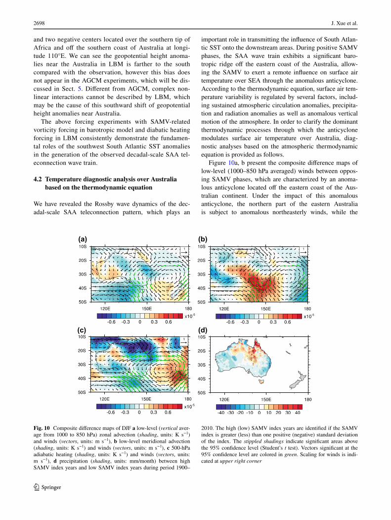
Figure 10a, b present the composite difference maps of low-level (1000–850 hPa averaged) winds between oppos-ing SAMV phases, which are characterized by an anoma-lous anticyclone located off the eastern coast of the Aus-tralian continent. Under the impact of this anomalous anticyclone, the northern part of the eastern Australia is subject to anomalous northeasterly winds, while the

(a) (b)

(c) (d)

Fig. 10 Composite difference maps of DJF a low-level (vertical aver-age from 1000 to 850  hPa) zonal advection (shading, units: K  s−1) and winds (vectors, units: m  s−1), b low-level meridional advection (shading, units: K s−1) and winds (vectors, units: m s−1), c 500-hPa adiabatic heating (shading, units: K  s−1) and winds (vectors, units: m  s−1), d precipitation (shading, units: mm/month) between high SAMV index years and low SAMV index years during period 1900–

2010. The high (low) SAMV index years are identified if the SAMV index is greater (less) than one positive (negative) standard deviation of the index. The stippled shadings indicate significant areas above the 95% confidence level (Student’s t test). Vectors significant at the 95% confidence level are colored in green. Scaling for winds is indi-cated at upper right corner

2699Decadal-scale teleconnection between South Atlantic SST and southeast Australia surface…

1 3

southern region of eastern Australia is influenced by north-westerly wind anomalies. To quantify the relative contribu-tion of each thermodynamic process associated with this anticyclone to the warming of surface air temperature over SEA during positive SAMV phases, composite analyses of terms on right-hand side of the thermodynamic equation between high SAMV index years and low SAMV index years are thus presented in Fig. 10. The composite differ-ence of low-level zonal advection shown in Fig.  10a pre-sents anomalous cold advection off the southern coast of the Australia, thus the zonal advection cannot explain the increased surface air temperature over SEA. For the com-posite difference map of low-level meridional advection term, significant warm advection anomaly is observed to be over SEA, which can be used to explain the increased surface air temperature over SEA during positive SAMV phases. These anomalous warm advection is associated with northwesterly winds prevailing over SEA, which can bring warmer air from the tropics to SEA. The third term on right hand side of the thermodynamic equation repre-sents adiabatic compression or expansion associated with the vertical motion of the atmosphere. Composite dif-ference map of the adiabatic heating term at 500  hPa is depicted in Fig. 10c, prominent adiabatic warming anomaly appears over areas covered by the anomalous anticyclone, this is because anticyclone is commonly accompanied with downward motion of air. The diabatic process can also play an important role in controlling surface air temperature. For example, precipitation anomalies can strongly modulate air temperature by modifying cloud cover and surface evapora-tion, the relationship between rainfall and air temperature over Australia has been noted in previous studies (Hendon et al. 2007; Power et al. 1998). Due to the lack of long-term reliable diabatic heating data, and in view of the important role of precipitation in diabatic processes, composite differ-ence of rainfall is employed to provide clues to difference in diabatic processes between opposing SAMV phases. We can see from Fig.  10d that composite difference map for summertime rainfall only shows small positive rain-fall anomaly in north-central Australia, and no significant rainfall difference between contrasting SAMV phases is observed in SEA.

Based on the above diagnostic analyses, we found the warming of surface air temperature over SEA during posi-tive SAMV phases is mainly caused by the anomalous meridional warm advection anomalies associated with the anomalous anticyclone near Australia. Therefore, the full physical image for the decadal-scale teleconnection between South Atlantic SST and summertime surface air temperature over SEA can be summarized as follows. Posi-tive SST anomalies in southwest South Atlantic can trigger the SAA teleconnection wave train, this wave train is char-acterized by an anomalous anticyclone over Australia, this

anticyclone can advect warm air from the tropics to SEA, and thus lead to the warming of surface air temperature there.

5 Decadal-scale teleconnection in SST-forced AGCM simulations

In preceding section, we have elucidated the Rossby wave dynamics for the generation of the decadal-scale SAA teleconnection pattern with simplified linear models and revealed the thermodynamics of how the SAA wave train can impact surface air temperature over SEA based on temperature diagnostics. To confirm the teleconnection mechanism, we still need to examine the decadal-scale tel-econnection between South Atlantic SST and summertime surface air temperature over SEA in more comprehensive AGCM experiments, which can include both the above dynamic and thermodynamic processes. Thus, a set of AMIP-style ensemble experiments carried out on the IFS AGCM with specified SST and sea–ice from HadISST2.1 is employed here to verify the decadal-scale teleconnection. Unlike individual model simulation that contains internal variability of the atmosphere, ensemble mean of a set of AGCM runs can be utilized to eliminate internal variability and highlight the SST-forced response of the atmosphere.

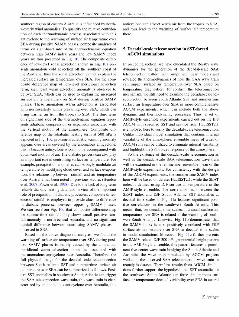
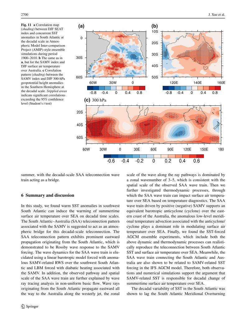
So the existence of the decadal-scale teleconnection as well as the decadal-scale SAA teleconnection wave train will be examined in the ten-member ensemble mean of the AMIP-style experiments. For consistency with the design of the AGCM experiments, the summertime SAMV index here will be based on dataset HadISST2.1, while the SEAT index is defined using DJF surface air temperature in the AMIP-style ensemble. The correlation map between the SEAT index and DJF South Atlantic SST anomalies at decadal time scales in Fig.  11a features significant posi-tive correlations in the southwest South Atlantic. This means that, on decadal time scales, increased surface air temperature over SEA is related to the warming of south-west South Atlantic. Likewise, Fig. 11b demonstrates that the SAMV index is also positively correlated with DJF surface air temperature over SEA at decadal time scales in model simulations. Moreover, Fig. 11c further presents the SAMV-related DJF 300-hPa geopotential height pattern in the AMIP-style ensemble, this pattern features a promi-nent five-center wave train bridging the South Atlantic and Australia, the wave train simulated by AGCM projects well onto the observed SAA teleconnection wave train in reanalysis dataset. Therefore, results from AGCM simula-tions further support the hypothesis that SST anomalies in the southwest South Atlantic can force simultaneous sur-face air temperature decadal variability over SEA in austral

2700 J. Xue et al.

1 3

summer, with the decadal-scale SAA teleconnection wave train acting as a bridge.

6 Summary and discussion

In this study, we found warm SST anomalies in southwest South Atlantic can induce the warming of summertime surface air temperature over SEA on decadal time scales. The South Atlantic–Australia (SAA) teleconnection pattern associated with the SAMV is suggested to act as an atmos-pheric bridge for this decadal-scale teleconnection. The SAA teleconnection pattern exhibits prominent eastward propagation originating from the South Atlantic, which is demonstrated to be Rossby wave response to the SAMV forcing. The wave dynamics for the SAA wave train is elu-cidated using a linear barotropic model forced with anoma-lous SAMV-related RWS over the southwest South Atlan-tic and LBM forced with diabatic heating associated with the SAMV. In addition, the observed pathway and spatial scale of the SAA wave train are further explained by wave ray tracing analysis in non-uniform basic flow. Wave rays originating from the South Atlantic propagate eastward all the way to the Australia along the westerly jet, the zonal

scale of the wave along the ray pathways is dominated by a zonal wavenumber of 3–5, which is consistent with the spatial scale of the observed SAA wave train. Then we further investigated thermodynamic processes, through which the SAA wave train can impact surface air tempera-ture over SEA based on temperature diagnostics. The SAA wave train driven by positive (negative) SAMV supports an equivalent barotropic anticyclone (cyclone) over the east-ern coast of the Australia, the anomalous low-level meridi-onal temperature advection associated with the anticyclone/cyclone plays a dominant role in modulating surface air temperature over SEA. Finally, we found the SST-forced AGCM ensemble experiments, which include both the above dynamic and thermodynamic processes can realisti-cally reproduce the teleconnection between South Atlantic SST and surface air temperature over SEA. Meanwhile, the SAA wave train connecting the South Atlantic and Aus-tralia are also shown to be related to SAMV-related SST forcing in the IFS AGCM model. Therefore, both observa-tions and numerical simulations support the argument that SAMV-related SST is responsible for decadal change of summertime surface air temperature over SEA.

The decadal variability of SST in the South Atlantic was shown to lag the South Atlantic Meridional Overturning

Fig. 11 a Correlation map (shading) between DJF SEAT index and concurrent SST anomalies in South Atlantic at the decadal scale in Atmos-pheric Model Inter-comparison Project (AMIP)-style ensemble simulations during period 1900–2010. b The same as in a, but for the SAMV index and DJF surface air temperature over Australia. c Correlation pattern (shading) between the SAMV index and DJF 300-hPa geopotential height anomalies in the Southern Hemisphere at the decadal scale. Stippled areas indicate significant correlations exceeding the 95% confidence level (Student’s t test)

(a) (b)

(c)

2701Decadal-scale teleconnection between South Atlantic SST and southeast Australia surface…

1 3

Circulation (SAMOC) by about 15–20  years (Lopez et  al. 2016b). In addition, expendable bathythermograph (XBT) transects between Cape Town and South America have been able to provide time series of the SAMOC for the first time since 2002 (Dong et  al. 2009; Garzoli et  al. 2013). When we accumulate sufficiently long time series of the SAMOC in the future, we may be able to predict the decadal-scale SST variation in the South Atlantic about 20 years in advance. And in view of the decadal-scale tel-econnection between South Atlantic SST and summertime surface air temperature over SEA revealed in this study, the SAMOC can be used to provide predictability for decadal variability of summertime surface air temperature over SEA.

Because SEA are suffering from the impacts of more and more frequent heat wave events under global warm-ing, heat extremes over Australia has received considerable attention from the climate research community (Alexan-der et al. 2006; Perkins et al. 2012). The mean-state tem-perature provides background for extreme events, and has a close relationship with the frequency of extremes (Purich et al. 2014). In this study, we have demonstrated that SST in South Atlantic can have a remote impact on the decadal change of seasonal mean surface air temperature over SEA in austral summer through the SAA wave train. A natural question is whether the variability of the South Atlantic can have a modulating effect on the heat wave events over SEA on decadal timescales by influencing mean-state surface air temperature. Thus, further analysis is needed to explore the possible impacts of South Atlantic on heat wave events over Australia in both historical observations and state-of-the-art coupled ocean–atmosphere general circulation models.

Acknowledgements The authors wish to thank Prof. Masahiro Watanabe for helpful suggestions in running the linear baroclinic model and anonymous reviewers for their constructive comments that significantly improved the quality of this paper. This work was jointly sponsored by MOST Key Project (2016YFA0601801) and SOA Inter-national Cooperation Program on Global Change and Air–Sea Inter-actions (GASI-IPOVAI-03, GASI-IPOVAI-06).

Open Access This article is distributed under the terms of the Creative Commons Attribution 4.0 International License (http://creativecommons.org/licenses/by/4.0/), which permits unrestricted use, distribution, and reproduction in any medium, provided you give appropriate credit to the original author(s) and the source, provide a link to the Creative Commons license, and indicate if changes were made.

References

Alexander L, Zhang X, Peterson T, Caesar J, Gleason B, Tank AK, Haylock M, Collins D, Trewin B, Rahimzadeh F, Tagipour A, Kumar K, Revadekar J, Griffiths G, Vincent L, Stephen-son D, Burn J, Aguilar E, Brunet M, Taylor M, New M, Zhai

P, Rusticucci M, Vazquez-Aguirre J (2006) Global observed changes in daily climate extremes of temperature and precipita-tion. J Geophys Res 111:D05109. doi:10.1029/2005JD006290

Ashcroft L, Karoly D, Gergis J (2012) Temperature variations of southeastern Australia, 1860–2011. Aust Meteorol Oceanogr J 62:227–245

Cai W, Rensch P, Cowan T, Hendon HH (2011) Teleconnection path-ways for ENSO and the IOD and the mechanism for impacts on Australian rainfall. J Clim 24:3910–3923. doi:10.1175/2011JCLI4129.1

Cui YF, Duan AM, Liu YM, Wu GX (2015) Interannual variability of the spring atmospheric heat source over the Tibetan Plateau forced by the North Atlantic SSTA. Clim Dyn 45:1617–1634. doi:10.1007/s00382-014-2417-9

Dima M, Lohmann G (2010) Evidence for two distinct modes of large-scale ocean circulation changes over the last century. J Clim 23:5–16. doi:10.1175/2009JCLI2867.1

Dong B, Dai A (2015) The influence of the Interdecadal Pacific Oscil-lation on temperature and precipitation over the globe. Clim Dyn 45:2667–2681. doi:10.1007/s00382-015-2500-x

Dong S, Garzoli S, Baringer M, Meinen C, Goni G (2009) Interan-nual variations in the Atlantic meridional overturning circu-lation and its relationship with the net northward heat trans-port in the South Atlantic. Geophys Res Lett 36:L20606. doi:10.1029/2009GL039356

Feng J, Li JP, Li Y (2010a) Is there a relationship between the SAM and southwest Western Australian winter rainfall? J Clim 23:6082–6089. doi:10.1175/2010JCLI3667.1

Feng J, Li JP, Li Y (2010b) A monsoon-like southwest Australian cir-culation and its relation with rainfall in southwest Western Aus-tralia. J Clim 23:1334–1353. doi:10.1175/2009JCLI2837.1

Feng J, Li JP, Li Y, Zhu JL, Xie F (2015) Relationships among the Monsoon-like Southwest Australian circulation, the south-ern annular mode, and winter rainfall over southwest West-ern Australia. Adv Atmos Sci 32:1063–1076. doi:10.1007/s00376-014-4142-z

Fierro AO, Leslie LM (2014) Relationships between southeast Aus-tralian temperature anomalies and large-scale climate drivers. J Clim 27:1395–1412. doi:10.1175/JCLI-D-13-00229.1

Garzoli SL, Baringer MO, Dong S, Perez RC, Yao Q (2013) South Atlantic meridional fluxes. Deep Sea Res Part I 71:21–32. doi:10.1016/j.dsr.2012.09.003

Gillett NP, Kell TD, Jones PD (2006) Regional climate impacts of the southern annular mode. Geophys Res Lett 33:L23704. doi:10.1029/2006GL027721

Gordon AL (1986) Interocean exchange of thermocline water. J Geo-phys Res 91(C4):50375046

Haarsma RJ, Campos EJD, Hazeleger W, Severijns C, Piola AR, Molteni F (2005) Dominant modes of variability in the South Atlantic: a study with a hierarchy of ocean–atmosphere models. J Clim 18:1719–1735. doi:10.1175/JCLI3370.1

Hansen AL, Bi P, Ryan P, Nitschke M, Pisaniello D, Tucker G (2008) The effect of heat waves on hospital admissions for renal disease in a temperate city of Australia. Int J Epidemiol 37:1359–1365

Hendon HH, Thompson DWJ, Wheeler MC (2007) Australian rainfall and surface temperature variations associated with the southern annular mode. J Clim 20:2452–2467. doi:10.1175/JCLI4134.1

Hersbach H, Peubey C, Simmons A et al (2015) ERA-20CM: a twen-tieth century atmospheric model ensemble. Q J R Meteorol Soc. doi:10.1002/qj.2

Hoskins BJ, Karoly DJ (1981) The steady linear response of a spheri-cal atmosphere to thermal and orographic forcing. J Atmos Sci 38:1179–1196

Hoskins BJ, Ambrizzi T (1993) Rossby-wave propagation on a real-istic longitudinally varying flow. J Atmos Sci 50(12):1661–1671

2702 J. Xue et al.

1 3

Huang B, Banzon VF, Freeman E, Lawrimore J, Liu W, Peter-son TC, Smith TM, Thorne PW, Woodruff SD, Zhang H-M (2015) Extended reconstructed sea surface temperature version 4 (ERSST.v4). Part I: upgrades and intercomparisons. J Clim 28:911–930. doi:10.1175/JCLI-D-14-00006.1

Hunter C, Binyamin J (2012) The impact of climate modes on sum-mer temperature and precipitation of Darwin, Australia, 1870–2011. Atmos Clim Sci 2:562–567. doi:10.4236/acs.2012.24051

Jones D, Trewin B (2000) On the relationships between the El Niño–Southern Oscillation and Australian land surface temperature. Int J Clim 20:697–719

Jones D, Wang W, Fawcett R (2009) High-quality spatial climate data-sets for Australia. Aust Meteorol Mag 58:233–248

Karoly D (2009) The recent bushfires and extreme heat wave in south-east Australia. Bull Aust Meteorol Oceanogr Soc 22:10–13

Latif M, Boning C, Willebrand J, Biastoch A, Dengg J, Keenlyside N, Schweckendiek U, Madec G (2006) Is the thermohaline circula-tion changing? J Clim 19:4631–4637

Legates DR, Willmott CJ (1990) Mean seasonal and spatial variability in global surface air temperature. Theor Appl Climatol 41:11–21. doi:10.1007/BF00866198

Lewis SC, Karoly DJ (2013) Anthropogenic contributions to Aus-tralia’s record summer temperatures of 2013. Geophys Res Lett 40:3705–3709. doi:10.1002/grl.50673

Li S, Bates GT (2007) Influence of the Atlantic multidecadal oscil-lation on the winter climate of East China. Adv Atmos Sci 24:126–135. doi:10.1007/s00376-007-0126-6

Li JP, Li Y, Feng J (2011) The characteristics of atmospheric cir-culation associated with austral winter rainfall in southwest Western Australia. Chin J Atmos Sci 35(5):801–817

Li JP, Feng J, Li Y (2012a) A possible cause of decreasing summer rainfall in northeast Australia. Int J Climatol 32:995–1005. doi:10.1002/joc.2328

Li Y, Li JP, Feng J (2012b) A teleconnection between the reduction of rainfall in southwest Western Australia and North China. J Clim 25:8444–8461

Li JP, Sun C, Jin FF (2013) NAO implicated as a predictor of North-ern Hemisphere mean temperature multidecadal variability. Geophys Res Lett 40:5497–5502. doi:10.1002/2013GL057877

Li Y, Li JP, Jin FF, Zhao S (2015) Interhemispheric propaga-tion of stationary rossby waves in a horizontally nonuniform background flow. J Atmos Sci 72:3233–3256. doi:10.1175/JAS-D-14-0239.1

Lopez H, Dong S, Lee SK, Campos E (2016a) Remote influence of Interdecadal Pacific Oscillation on the South Atlantic meridi-onal overturning circulation variability. Geophys Res Lett 43:8250–8258

Lopez H, Dong S, Lee SK, Goni G (2016b) Decadal modulations of interhemispheric global atmospheric circulations and monsoons by the South Atlantic meridional overturning circulation. J Clim 29:1831–1851. doi:10.1175/JCLI-D-15-0491.1

Meneghini B, Simmonds I, Smith IN (2007) Association between Australian rainfall and the southern annular mode. Int J Climatol 27:109–121. doi:10.1002/joc.1370

Morak S, Hegerl GC, Christidis N (2013) Detectable changes in the frequency of temperature extremes. J Clim 26:1561–1574. doi:10.1175/JCLI-D-11-00678.1

Morioka Y, Tozuka T, Yamagata Y (2011) On the growth and decay if the subtropical dipole mode in the South Atlantic. J Clim. doi:10.1175/2011JCLI4010.1

Murphy B, Timbal B (2008) A review of recent climate variability and climate change in southeastern Australia. Int J Climatol 28:859–879. doi:10.1002/joc.1627

Nnamchi HC, Li J, Anyadike RNC (2011) Does a dipole mode really exist in the South Atlantic Ocean? J Geophys Res 116:D15104. doi:10.1029/2010JD015579

Nnamchi HC, Li J, Kucharski F et al (2016) An equatorial–extratropi-cal dipole structure of the Atlantic Niño. J Clim 29:7295–7311. doi:10.1175/JCLI-D-15-0894.1

Parker D, Folland C, Scaife A, Knight J, Colman A, Baines P, Dong B (2007) Decadal to multidecadal variability and the climate change background. J Geophys Res 112:D18115. doi:10.1029/2007jd008411

Peng S, Whitaker JS (1999) Mechanisms determining the atmospheric response to midlatitude SST anomalies. J Clim 12:1393–1408

Perkins SE, Alexander LV, Nairn JR (2012) Increasing frequency, intensity and duration of observed heatwaves and warm spells. Geophys Res Lett 39:L20714. doi:10.1029/2012GL053361

Poli P, Hersbach H, Dee DP (2016) ERA-20C: an atmospheric reanal-ysis of the twentieth century. J Clim 29:4083–4097. doi:10.1175/JCLI-D-15-0556.1

Power S, Tseitkin F, Torok SJ, Lavery B, Dahni R, McAveny B (1998) Australian temperature, Australian rainfall and the Southern Oscillation, 1910–1992: coherent variability and recent changes. Aust Meteorol Mag 47:85–101

Power S, Casey T, Folland C, Colman A, Mehta V (1999) Interdec-adal modulation of the impact of ENSO on Australia. Clim Dyn 15:219–324

Purich A, Cowan T, Cai W, van Rensch P, Uotila P, Pezza A, Boschat G, Perkins S (2014) Atmospheric and oceanic conditions associ-ated with Southern Australian heat waves: a CMIP5 analysis. J Clim 27(20):7807–7829. doi:10.1175/JCLI-D-14-00098.1

Rayner NA et  al (2013) The Met Office Hadley Centre sea ice and sea-surface temperature data set, version 2, part 3: the combined analysis (in preparation)

Risbey JS, Pook MJ, McIntosh PC, Wheeler MC, Hendon HH (2009) On the remote drivers of rainfall variability in Australia. Mon Weather Rev 137:3233–3253. doi:10.1175/2009MWR2861.1

Robertson AW, Farrara JD, Mechoso CR (2003) Simulations of the atmospheric response to South Atlantic sea surface temperature anomalies. J Clim 16:2540–2551

Sardeshmukh PD, Hoskins BJ (1988) The generation of global rota-tional flow by steady idealized tropical divergence. J Atmos Sci 45:1228–1251

Sterl A, Hazeleger W (2003) Coupled variability and air–sea interac-tion in the South Atlantic Ocean. Clim Dyn 21:559–571

Stocker T, Qin D, Plattner G-K, Tignor M, Allen SK, Boschung J, Nauels A, Xia Y, Bex V, Midgley PM (2014) Climate change 2013: the physical science basis. Cambridge University Press, Cambridge

Sun C, Li JP, Jin FF, Ding QR (2013) Sea surface temperature inter-hemispheric dipole and its relation to tropical precipitation. Environ Res Lett. doi:10.1088/1748-9326/8/4/044006

Sun C, Li JP, Feng J, Xie F (2015a) A decadal-scale teleconnection between the North Atlantic Oscillation and subtropical east-ern Australian rainfall. J Clim 28:1074–1092. doi:10.1175/JCLI-D-14-00372.1

Sun C, Li JP, Jin FF (2015b) A delayed oscillator model for the quasi-periodic multidecadal variability of the NAO. Clim Dyn. doi:10.1007/s00382-014-2459-z

Sun C, Li JP, Zhao S (2015c) Remote influence of Atlantic multidec-adal variability on Siberian warm season precipitation. Sci Rep. doi:10.1038/srep16853

Sun C, Li JP, Ding RQ, Jin Z (2016) Cold season Africa-Asia multidecadal teleconnection pattern and its relation to the Atlantic multidecadal variability. Clim Dyn. doi:10.1007/s00382-016-3309-y

Takaya K, Nakamura H (2001) A formulation of a phase-independent wave-activity flux for stationary and migratory quasigeostrophic eddies on a zonally varying basic flow. J Atmos Sci 58:608–627

2703Decadal-scale teleconnection between South Atlantic SST and southeast Australia surface…

1 3

Taschetto AS, England MH (2009) El Niño Modoki impacts on Australian Rainfall. J Clim 22:3167–3174. doi:10.1175/2008jcli2589.1

Ummenhofer CC et al (2011) Indian and Pacific Ocean influences on southeast Australian drought and soil moisture. J Clim 24:1313–1336. doi:10.1175/2010JCLI3475.1

Vellinga M, Wood RA (2002) Global climatic impacts of a collapse of the Atlantic thermohaline circulation. Clim Change 54:251–267

Venegas SA, Mysak LA, Straub DN (1997) Atmosphere–ocean cou-pled variability in the South Atlantic. J Clim 10:2904–2920

Verdon DC, Wyatt AM, Kiem AS, Franks SW (2004) Multidecadal variability of rainfall and streamflow: Eastern Australia. Water Resour Res 40:W10201. doi:10.1029/2004WR003234

Wainer I, Soares J (1997) North-northeast Brazil rainfall and its dec-adal-scale relationship to wind stress and sea surface tempera-ture. Geophys Res Lett 24:277–280

Wainer I, Venegas SA (2002) South Atlantic multidecadal variability in the climate system model. J Clim 15:1408–1420

Wang C, Zhang L, Lee S-K et  al (2014) A global perspective on CMIP5 climate model biases. Nat Clim Change 4:201–205. doi:10.1038/nclimate2118

Watanabe M (2004) Asian jet waveguide and a downstream extension of the North Atlantic Oscillation. J Clim 17:4674–4691

Watanabe M, Kimoto M (2000) Atmosphere–ocean thermal coupling in the North Atlantic: a positive feedback. Q J R Meteorol Soc 126:3343–3369

Watterson IG (2009) Components of precipitation and temperature anomalies and change associated with modes of the Southern Hemisphere. Int J Climatol 29:809–826. doi:10.1002/joc.1772

Wu Z, Wang B, Li J, Jin F-F (2009) An empirical seasonal predic-tion model of the East Asian summer monsoon using ENSO and NAO. J Geophys Res 114:D18120. doi:10.1029/2009JD011733

Zhao S, Li JP, Li Y (2015) Dynamics of an interhemispheric tel-econnection across the critical latitude through a southerly duct during boreal winter. J Clim 28:7437–7456. doi:10.1175/JCLI-D-14-00425.1

Zhou YF, Wu ZW (2016) Possible impacts of mega-El Niño/Southern oscillation and Atlantic multidecadal oscillation on Eurasian heat wave frequency variability. Q J R Meteorol Soc 142:1647–1661. doi:10.1002/qj.2759