___________________________________________________________________________

2008/SOM3/ISTWG/SYM/004 Agenda Item: 1-01

How Well Are Southern Hemisphere Teleconnection Patterns Predicted by Seasonal Climate Models?

Submitted by: University of São Paulo

APEC Climate SymposiumLima, Peru

19-21 August 2008

19 August, 2008 APEC Climate Symposium, 2008

Abstract 1-01

How well are Southern Hemisphere teleconnection patterns predicted by seasonal climate models?

Tércio Ambrizzi

Department of Atmospheric Sciences University of São Paulo - Brazil

The identification of teleconnection patterns and the analysis of their effect on the horizontal

structure of the atmospheric circulation can be very useful to understand anomalous events in many

regions of the world. Local forcing in specific places can influence remote regions through organized

structures in form of waves. One way to analyze this wave propagation is using the stationary Rossby

wave linear theory in a barotropic atmosphere. Previous studies on atmospheric teleconnection

patterns have shown that linear wave theory may explain some of the observed low-frequency

variability. Using a climatological December-January-February (DJF) basic flow and a simple

barotropic model, it is possible to examine the preferred trajectories followed by Rossby waves

around the globe. For instance, through the analysis of climatological stationary wavenumber fields

(Ks) it can be demonstrated that the upper level tropospheric jets can act as waveguides in the

atmosphere. In particular, during the Southern Hemisphere winter (June-July-August – JJA), some

studies have numerically demonstrated, using a barotropic model, that the subtropical and polar jets

have such characteristic. One can suggest that the atmospheric dynamics at large scales can be

qualitatively interpreted through the linear wave theory.

The teleconnection analyses described above were applied to 10 years of ECMWF ensemble

forecasts. The basic theory related to dynamical systems can give an insight into the predictability of

large events and could be used to improve the seasonal forecasting. Preliminary results have

identified a large variability among the ensemble members to represent the circulation patterns in a

three month forecast. This research is part of a multi-institutional collaboration proposal called

EUROBRISA which one of its objectives is to provide not only the Brazilian government but also other

South American local governments improved and well-calibrated seasonal forecasts.

1

How well are Southern Hemisphere teleconnection patterns predicted

by seasonal climate models?

Tércio AmbrizziDepartment of Atmospheric Science - USP

APEC Climate Symposium Lima/2008

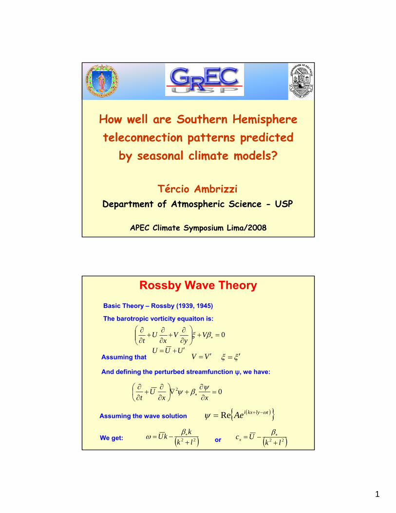
Rossby Wave Theory

The barotropic vorticity equaiton is:

0=+⎟⎟⎠

⎞⎜⎜⎝

⎛∂∂

+∂∂

+∂∂

∗βξ Vy

Vx

Ut

UUU ′+=VV ′= ξξ ′=

02 =∂∂

+∇⎟⎠⎞

⎜⎝⎛

∂∂

+∂∂

∗ xxU

tψβψ

( ){ }tlykxiAe ωψ −+= Re

( )22 lkkkU+

−= ∗βω ( )22 lkUcx +

−= ∗β

Basic Theory – Rossby (1939, 1945)

Assuming that

And defining the perturbed streamfunction ψ, we have:

Assuming the wave solution

We get: or

2

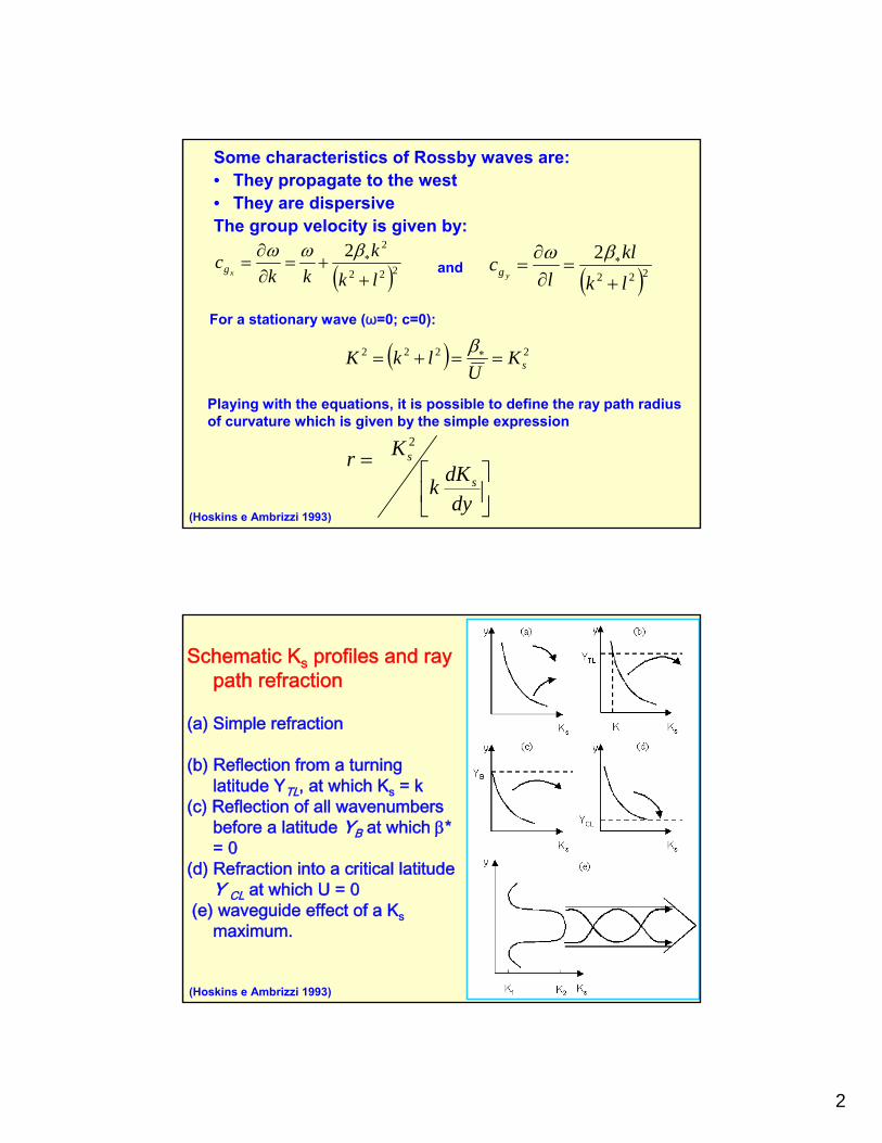
Some characteristics of Rossby waves are:• They propagate to the west• They are dispersiveThe group velocity is given by:

( )222

22lkk

kkc

xg+

+=∂∂

= ∗βωω

( )222

2lkkl

lc

yg+

=∂∂

= ∗βω

For a stationary wave (ω=0; c=0):

( ) 2222sK

UlkK ==+= ∗β

⎥⎦

⎤⎢⎣

⎡=

dydKk

Krs

s2

and

Playing with the equations, it is possible to define the ray path radius of curvature which is given by the simple expression

(Hoskins e Ambrizzi 1993)

Schematic Ks profiles and ray path refraction

(a) Simple refraction

(b) Reflection from a turning latitude YTL, at which Ks = k

(c) Reflection of all wavenumbersbefore a latitude YB at which β* = 0

(d) Refraction into a critical latitude Y CL at which U = 0

(e) waveguide effect of a Ksmaximum.

(Hoskins e Ambrizzi 1993)

3

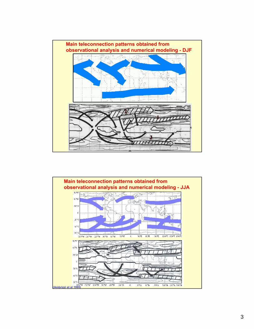
Main teleconnection patterns obtained from observational analysis and numerical modeling - DJF

Main teleconnection patterns obtained fromobservational analysis and numerical modeling - JJA

(Ambrizzi et al 1995)

4

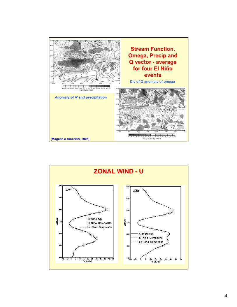
Stream Function, Omega, Precip and Q vector - average

for four El Niño events

Anomaly of Ψ and precipitation

Div of Q anomaly of omega

(Magaña e Ambrizzi, 2005)

ZONAL WIND - U

5

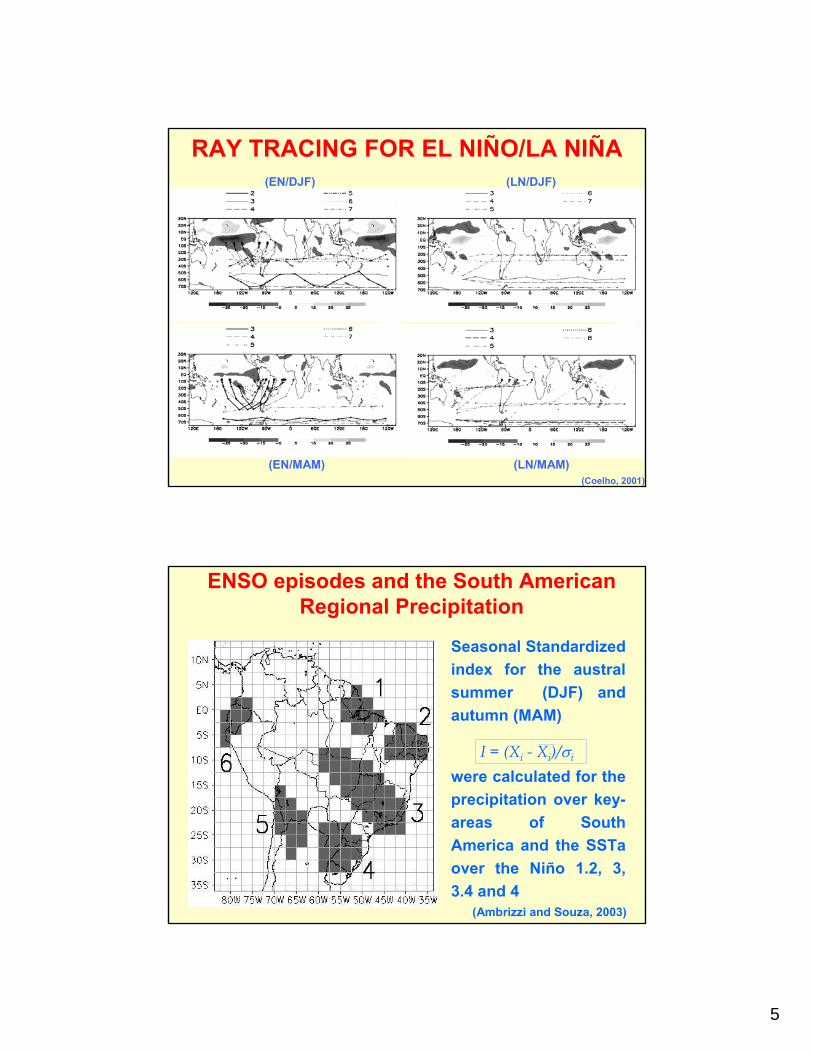
RAY TRACING FOR EL NIÑO/LA NIÑA(EN/DJF) (LN/DJF)

(EN/MAM) (LN/MAM)(Coelho, 2001)

I = (Xi - Xi)/σi

ENSO episodes and the South American Regional Precipitation

Seasonal Standardized index for the austral summer (DJF) and autumn (MAM)

were calculated for the precipitation over key-areas of South America and the SSTa over the Niño 1.2, 3, 3.4 and 4

(Ambrizzi and Souza, 2003)

6

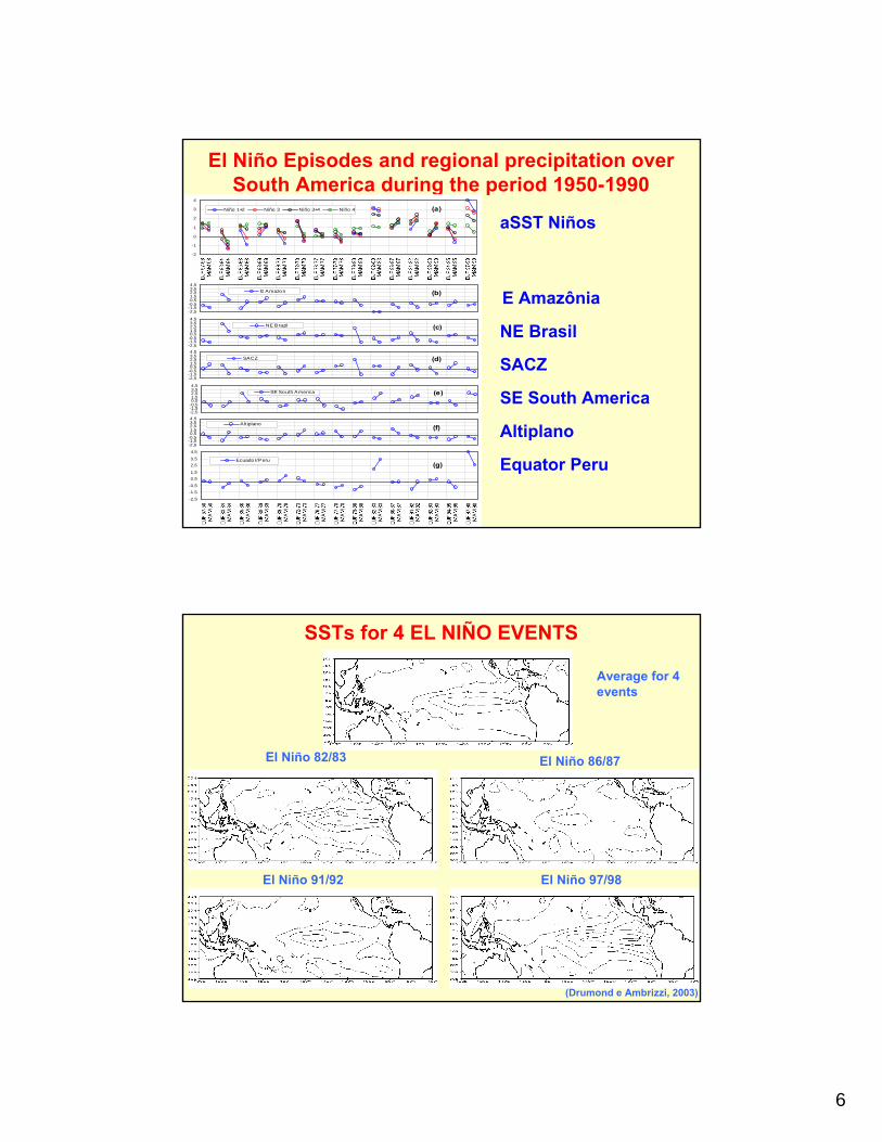
El Niño Episodes and regional precipitation over South America during the period 1950-1990

(g)

-2,5

-1,5-0,5

0,51,5

2,53,5

4,5

Ecuador/Peru

(f)

-2,5-1,5-0,50,51,52,53,54,5

Altiplano

(e)

-2,5-1,5-0,50,51,52,53,54,5

SE South America

(d)

-2,5-1,5-0,50,51,52,53,54,5

SACZ

(c)

-2,5-1,5-0,50,51,52,53,54,5

NE Brazil

(b)

-2,5-1,5-0,50,51,52,53,54,5

E Amazon

(a)

-2

-1

0

1

2

3

4

Niño 1+2 Niño 3 Niño 3+4 Niño 4

aSST Niños

E Amazônia

NE Brasil

SACZ

SE South America

Altiplano

Equator Peru

SSTs for 4 EL NIÑO EVENTS

El Niño 82/83 El Niño 86/87

El Niño 91/92 El Niño 97/98

Average for 4 events

(Drumond e Ambrizzi, 2003)

7

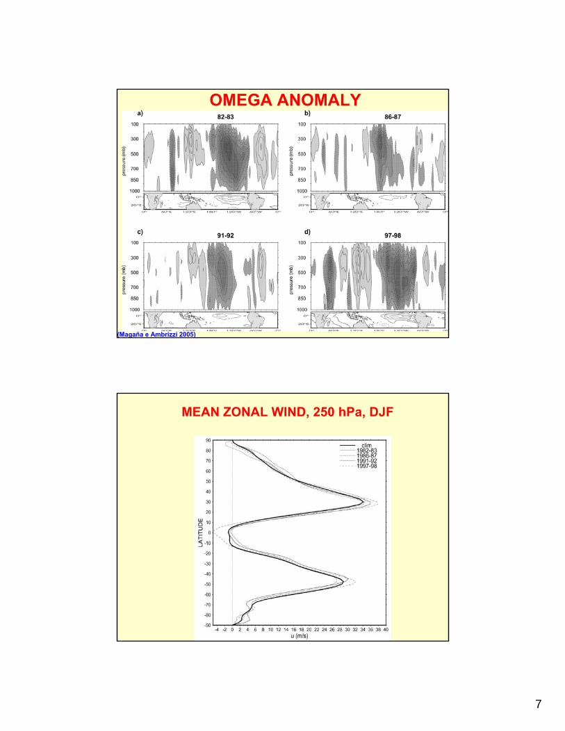
OMEGA ANOMALY

(Magaña e Ambrizzi 2005)

MEAN ZONAL WIND, 250 hPa, DJF

8

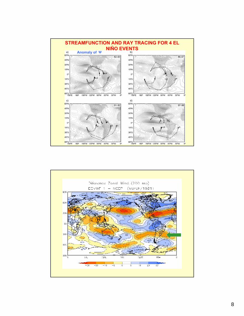
STREAMFUNCTION AND RAY TRACING FOR 4 EL NIÑO EVENTS

Anomaly of Ψ

9

NCEP

NCEP

NCEP

NCEP

10

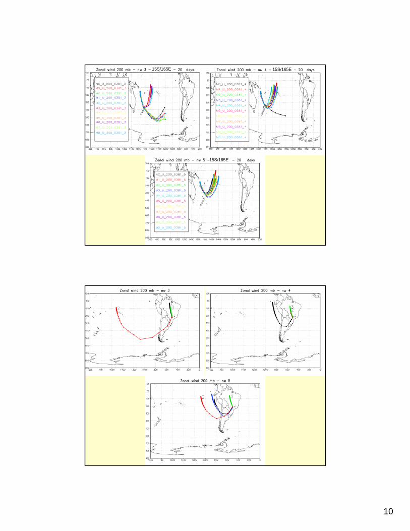
15S/165E

15S/165E 15S/165E

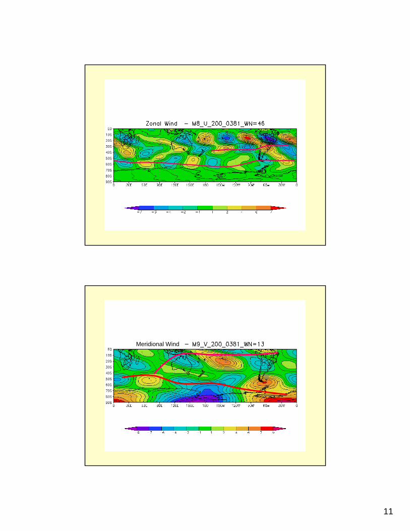
11

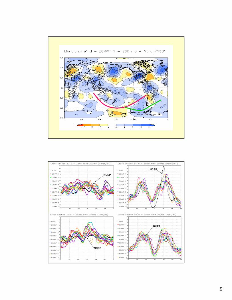
Meridional Wind

12

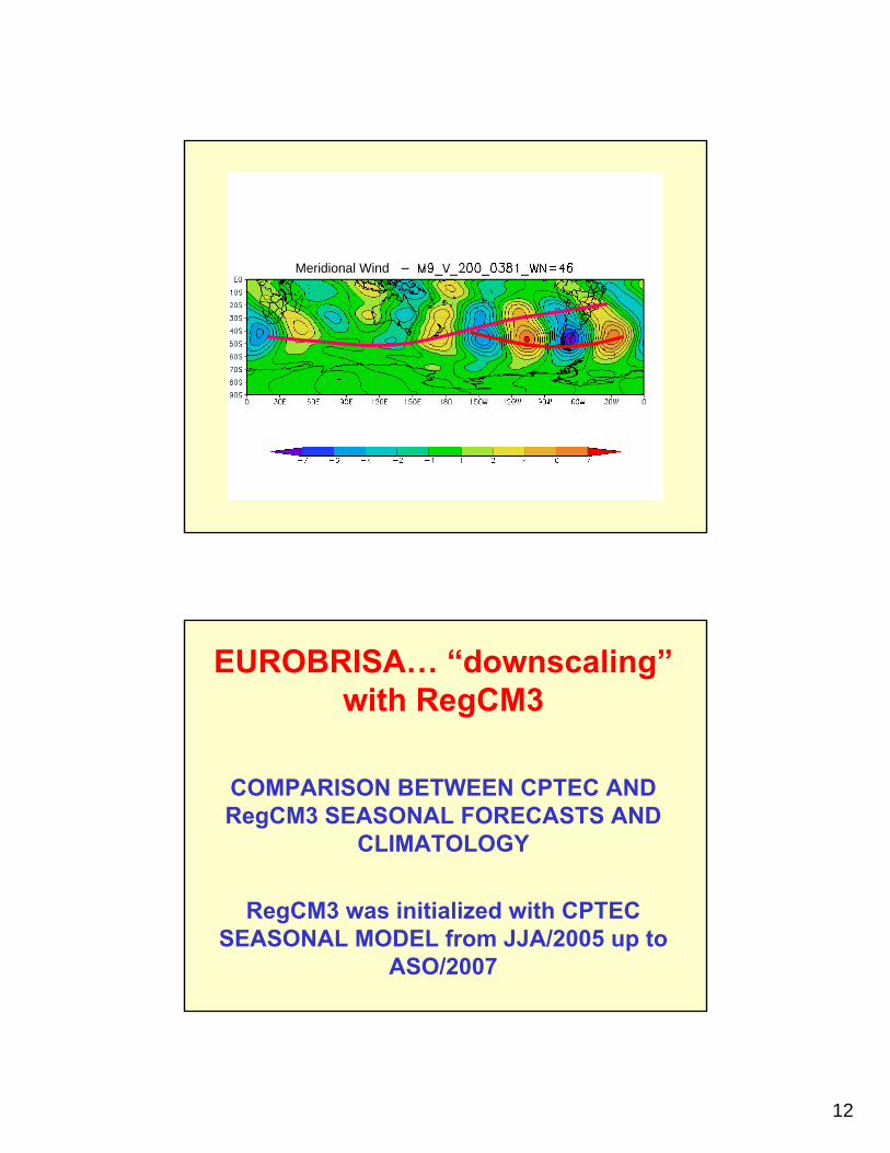
Meridional Wind

EUROBRISA… “downscaling”with RegCM3

COMPARISON BETWEEN CPTEC AND RegCM3 SEASONAL FORECASTS AND

CLIMATOLOGY

RegCM3 was initialized with CPTEC SEASONAL MODEL from JJA/2005 up to

ASO/2007

13

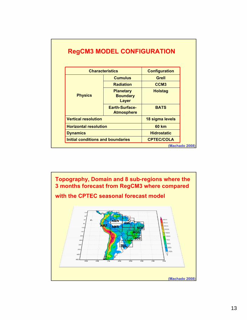
CPTEC/COLAInitial conditions and boundariesHidrostaticDynamics

60 kmHorizontal resolution

18 sigma levelsVertical resolution

BATSEarth-Surface-Atmosphere

HolstagPlanetary Boundary

Layer

CCM3RadiationGrellCumulus

Physics

ConfigurationCharacteristics

RegCM3 MODEL CONFIGURATION

(Machado 2008)

AMZNDE

SDE

SUL

AMN

AMSAML

MGS

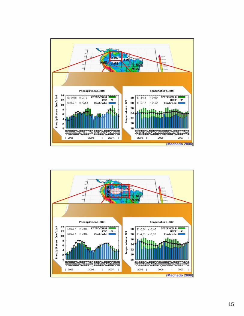
Topography, Domain and 8 sub-regions where the 3 months forecast from RegCM3 where compared

with the CPTEC seasonal forecast model

(Machado 2008)

14

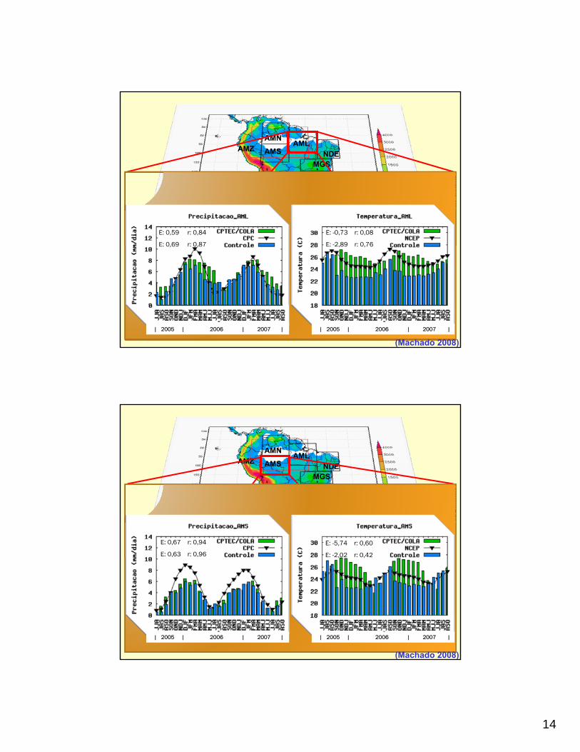
AMZNDE

SDE

SUL

AMN

AMSAML

MGS

E: -0,73 r: 0,08

E: -2,89 r: 0,76

| 2005 | 2006 | 2007 |

E: 0,59 r: 0,84

E: 0,69 r: 0,87

| 2005 | 2006 | 2007 |

(Machado 2008)

AMZNDE

SDE

SUL

AMN

AMSAML

MGS

E: 0,67 r: 0,94

E: 0,63 r: 0,96

E: -5,74 r: 0,60

E: -2,02 r: 0,42

| 2005 | 2006 | 2007 | | 2005 | 2006 | 2007 |

(Machado 2008)

15

AMZNDE

SDE

SUL

AMN

AMSAML

MGS

E: -0,05 r: 0,73

E: 0,27 r: 0,53

E: -14,8 r: 0,69

E: -27,7 r: 0,10

| 2005 | 2006 | 2007 | | 2005 | 2006 | 2007 |

(Machado 2008)

NDE

SDE

SUL

MGS

E: 0,77 r: 0,91

E: 0,77 r: 0,91

E: -6,5 r: 0,46

E: -7,7 r: 0,55

| 2005 | 2006 | 2007 | | 2005 | 2006 | 2007 |

(Machado 2008)

16

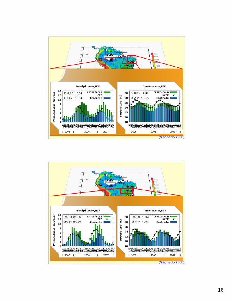
AMZNDE

SDE

SUL

AMN

AMSAML

MGS

E: -1,86 r: 0,64

E: 0,62 r: 0,84

E: -0,05 r: 0,30

E: -2,14 r: 0,90

| 2005 | 2006 | 2007 | | 2005 | 2006 | 2007 |

(Machado 2008)

AMZNDE

SDE

SUL

AMN

AMSAML

MGS

E: 0,33 r: 0,85

E: 0,56 r: 0,80

E: 0,08 r: 0,67

E: -0,44 r: 0,64

| 2005 | 2006 | 2007 | | 2005 | 2006 | 2007 |

(Machado 2008)

17

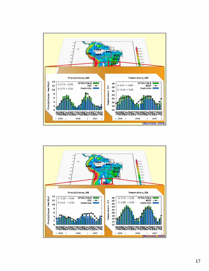
AMZNDE

SDE

SUL

AMN

AMSAML

MGS

E: 0,74 r: 0,92

E: 0,75 r: 0,91E: 0,57 r: 0,89

E: -0,10 r: 0,85

| 2005 | 2006 | 2007 | | 2005 | 2006 | 2007 |

(Machado 2008)

AMZNDE

SDE

SUL

AMN

AMSAML

MGS

| 2005 | 2006 | 2007 | | 2005 | 2006 | 2007 |

E: -0,26 r: 0,64

E: 0,13 r: 0,63

E: 0,74 r: 0,95

E: 0,86 r: 0,94

(Machado 2008)

18

Thanks to Dr. Thanks to Dr. SajiSaji N. N. HameedHameed and the APEC Climate and the APEC Climate

Center for the invitation.Center for the invitation.

GRUPO DE ESTUDOS CLIMÁTICOS

THANK YOU FOR YOUR ATTENTIONTHANK YOU FOR YOUR ATTENTION

GRACIAS POR SU ATENCIGRACIAS POR SU ATENCIÓÓNN

CLIMATE STUDIES GROUP