Decadal Variability in Coupled Sea-Ice–Thermohaline ...research.atmos.ucla.edu/csi/REF/pdfs/newice.pdftem. Since the THC involves long timescales, it is po-tentially a rich source

DECEMBER 1997 3059Y A N G A N D N E E L I N

q 1997 American Meteorological Society

Decadal Variability in Coupled Sea-Ice–Thermohaline Circulation Systems*

JIAYAN YANG

Department of Physical Oceanography, Woods Hole Oceanographic Institution, Woods Hole, Massachusetts

J. DAVID NEELIN

Department of Atmospheric Sciences and Institute of Geophysics and Planetary Physics, University of California,Los Angeles, Los Angeles, California

(Manuscript received 27 September 1996, in final form 10 March 1997)

ABSTRACT

An interdecadal oscillation in a coupled ocean–ice system was identified in a previous study. This paperextends that study to further examine the stability of the oscillation and the sensitivity of its frequency to variousparameters and forcing fields. Three models are used: (i) an analytical box model; (ii) a two-dimensional modelfor the ocean thermohaline circulation (THC) coupled to a thermodynamic ice model, as in the authors’ previousstudy; (iii) a three-dimensional ocean general circulation model (OGCM) coupled to a similar ice model. Thebox model is used to elucidate the essential feedbacks that give rise to this oscillation and to identify the mostimportant parameters and processes that determine the period. Numerical experiments in the 2D THC–ice modelshow that the model stability is sensitive to the ocean–ice coupling coefficient, the eddy diffusivity, and thestrength of the thermohaline-circulation feedback per unit surface-polar density perturbation. The coupled modelbecomes more stable toward low coupling, greater diffusion, and weaker THC feedback. The period of theoscillation is less sensitive to these parameters. Nonlinear effects in the sea-ice model become important in thehigher ocean–ice coupling regime where the effective sea-ice damping associated with this nonlinearity stabilizesthe model. Surface Newtonian damping is also tested. The 3D OGCM, which includes both wind stress andbuoyancy forcings, is used to test this coupled ocean–ice mechanism in a more realistic model setting. Thismodel generates an interdecadal oscillation whose characteristics and phase relations among the model variablesare similar to the oscillation obtained in the 2D models. The major difference is that the oscillation frequencyis considerably lower. This difference can be explained in terms of the analytical box model solution in whichthe period of the oscillation depends on the rate of anomalous density production by melting/cooling of sea iceper SST anomaly, times the rate of warming/cooling by anomalous THC heat advection per change in densityanomaly. The 3D model has a smaller THC response to high-latitude density perturbations than in the 2D model,and anomalous velocities in the 3D case tend to follow the mean isotherms so the anomalous heat advection isreduced. This slows the ocean–ice feedback process, leading to the longer oscillation period.

1. Introduction

Interdecadal variations of oceanic temperature andsalinity, and sea-ice extent in the North Atlantic Oceanare major signals in the marine climate system (Dicksonet al. 1988; Mysak et al. 1990; Walsh and Chapman1990). Notable variations include the Great SalinityAnomaly (GSA) in the North Atlantic Ocean in the1970s (Mysak et al. 1990; Dickson et al. 1988). Recentanalyses also reveal apparent quasi-oscillatory modes

* Woods Hole Oceanographic Institution Contribution Number9409.

Corresponding author address: Dr. Jiayan Yang, Dept. of PhysicalOceanography, Woods Hole Oceanographic Institution, Woods Hole,MA 02543.E-mail: [email protected]

with interdecadal timescales in the North Atlantic(Kushnir 1994; Deser and Blackmon 1993) and globally(Ghil and Vautard 1991). Numerical models have sug-gested potential mechanisms for decadal oscillations as-sociated with the thermohaline circulation (THC) (e.g.,Weaver et al. 1991; Winton and Sarachik 1993; Del-worth et al. 1993; Huang 1993, 1994; Chen and Ghil1995). Such climate variations may result from inter-actions among different components of the climate sys-tem. Since the THC involves long timescales, it is po-tentially a rich source for such low-frequency variations.The THC variability is primarily controlled by thosephysical processes that determine the sea surface tem-perature (SST) and salinity (SSS) at the subpolar NorthAtlantic Ocean where deep water is formed. The pres-ence of sea ice not only changes the surface heat fluxbut also modifies the surface freshwater flux. Sea ice isthus postulated to play an important role in the THC-related climate variations. The objective of this paper

3060 VOLUME 10J O U R N A L O F C L I M A T E

is to explore important feedbacks in the THC–sea-icecoupled system by using a hierarchy of models.

In a previous study, we suggested that a mechanismthat involves active ocean–ice interaction may contrib-ute to such variability (Yang and Neelin 1993, hereafterYN93). This paper extends the study of YN93 to ex-amine this oscillation over a broad range of parametersand forcing fields, and to test it in a more realistic three-dimensional primitive equation model. This paper alsopresents an analytical solution to elucidate the essentialphysics of the oscillation. The effect of nonlinearity ofthe sea-ice model will also be discussed.

In the next section, models used in this study, in-cluding a two-dimensional THC model, a three-dimen-sional ocean general circulation model, and a thermo-dynamic sea-ice model, will be introduced. The solutionof an analytical box model will be studied in section 3to highlight the essential feedbacks that give rise to thistype of oscillation. The sensitivity of this model to var-ious physical parameters and forcings will be discussedin section 4 by using the same two-dimensional modelas that in YN93. Results from the three-dimensionalmodel will be discussed in section 5.

2. Models

a. A two-dimensional THC model

The zonally averaged THC model of YN93 is usedto calculate the oceanic temperature, salinity, and ve-locity. The overturning circulation is driven by the me-ridional density gradient, that is,

4 4] c ] c g ]rA 1 A 5 , (1)V H4 2 2]z ]y ]z r ]y0

where c is the streamfunction; AV and AH are the verticaland horizontal eddy viscosities, respectively; r is thewater density; and g is the gravitational accelerationrate.

The temperature and salinity are determined by ad-vection and mixing:

2 2]T ](yT) ](wT) ] T ] T1 1 5 k 1 k (2)H V2 2]t ]y ]z ]y ]z

2 2]S ](yS) ](wS) ] S ] S1 1 5 k 1 k , (3)H V2 2]t ]y ]z ]y ]z

where kH and kV are horizontal and vertical diffusioncoefficients. The model domain extends from 708S to708N with a constant depth of 4000 m. The model res-olution is 28 in the horizontal and 200 m in the vertical.Equations (1)–(3) are solved numerically, using bound-ary conditions of no-normal flow and no-normal flux atall rigid walls. No wind stress is applied at the surface.The so-called mixed boundary condition is used at thesurface, in which the SST is dampened toward a pre-scribed equilibrium state while a virtual salt flux is ap-plied to approximate the freshwater flux:

]T k (T 2 T) if d 5 0aw erC k 5 (4)p V 5]z k (T 2 T) if d . 0iw f

]S ]dk 5 F(y) 1 S , (5)V 01 2]z ]t

where Te is a prescribed equilibrium temperature for theair–sea heat flux, which decreases sinusoidally from278C at the equator to the seawater freezing temperatureT f 5 228C at the ice edge; kaw is the air–sea heat fluxcoefficient; and kiw is the water–ice heat flux coefficient,which is usually smaller than kaw; F( y) is specified asan approximation to the evaporation-minus-precipita-tion rate; d is the ice thickness; and S0 is the meansurface salinity.

YN93 used a linear equation of state, that is, r 5r0(1 2 aT 1 bS) with a 5 2 3 1024 8C21 and b 5 83 1024 psu21. The real equation of state is highly non-linear in temperature. For example, the United NationsEducational, Scientific, and Cultural Organization(UNESCO) equation of state (Gill 1982) estimates that]r/]T varies from 20.3 kg 8C21 at 258C to 20.026 kg8C21 at 228 for S 5 35 psu. Therefore, we include anonlinear equation of state in this study. Following Win-ton and Sarachik (1993) we use a third-order polynomialapproximation to the UNESCO equation:

2r(T, S) 5 0.7968S 2 0.0559T 2 0.0063T25 31 3.7315 3 10 T . (6)

One of the most noticeable differences in using (6),as opposed to the linear equation in YN93, is that theoverall THC strength is considerably weaker under thesame forcing. The overturning cell is dominated by thethermal mode, and thus its strength is controlled to alarge extent by the meridional density contrast contrib-uted by temperature gradient. The use of (6) greatlyreduces that temperature contribution to r in cold water.We adjust the values of AV and AH such that the modelproduces about 15 sverdrups (106 m3 s21) of deep water.

Like many other THC models, the ocean model (1)–(3) with boundary conditions (4) and (5) produces mul-tiple equilibria under hemispherically symmetric forc-ings. The symmetric two-cell circulation is unstable tofinite-amplitude perturbations and can be shifted to amore stable one-cell circulation, such as Fig. 1 shownin YN93, with sinking near the northern boundary andupwelling elsewhere.

b. The three-dimensional model

The three-dimensional ocean model used in this studyis the Geophysical Fluid Dynamics Laboratory (GFDL)Modular Ocean Model (MOM) (Pacanowski et al.1993). The model physics, as described by Bryan(1969), uses the hydrostatic and Boussinesq approxi-mations and a nonlinear equation of state. The numericalschemes are discussed in detail in Pacanowski et al.


FIG. 1. Schematic of the box model.

(1993). In our application, a mixed boundary conditionis used, in which the SST is relaxed toward the zonallyaveraged SST climatology of Levitus (1982), and thevirtual salt flux is diagnosed from a steady state obtainedby restoring the SSS to Levitus’s salinity climatology.The model domain extends from 108 to 758N. As wewill discuss later in section 4, the coupled ocean–iceoscillation arising from using a half-basin model is quitesimilar to that using a full-basin model. Thus, the resultsfrom this half-basin model can be extended to a largerdomain. Because long simulations are needed for eachrun, we decided to use a rather coarse resolution of 483 48 in the horizontal. A vertical depth of 4500 m isdivided into 15 levels in thickness increments from 30m at the surface to 630 m at the bottom. The relaxationtime for the surface heat flux is 30 days.

c. A thermodynamic sea-ice model

The sea-ice model used in this study is the same asthat used by Yang and Neelin (1996) and Zhang et al.(1995). This model, originally constructed by Welander(1977), is similar to that of Maykut and Untersteiner(1971). YN93 used this model to derive the linearizedice model used there. The detailed derivation can befound in these previous papers. Here we present only abrief description of how changes in the heat budget leadto freezing and melting.

Major heat fluxes at the upper surface of sea ice in-clude solar radiation (Fr); longwave radiation from theatmosphere (FL); reflected solar radiation (aFr), wherea is the surface albedo; outgoing radiation («Ls ),4T s

where «L is the longwave emissivity, s is the Stefan–Boltzmann constant, and Ts is the surface temperatureof sea ice; and heat conduction [2Ki(dT/dz)z50], whereKi is the thermal conductivity. In addition, there areseveral smaller fluxes, such as sensible heat flux (Fs),latent heat flux (Fl), and the penetrating radiative fluxthrough the surface (I0). Since the seasonal cycle is ex-cluded in our model, we assume that the upper surfacetemperature of sea ice is always below the freezing pointand no melting occurs at the upper surface. As discussedin Maykut and Untersteiner (1971) and in Thorndike

(1992), a balance of the major heat fluxes at the uppersurface takes the form

dT4(1 2 a)F 2 I 1 F 2 « sT 1 K 5 0. (7)T 0 L L s i1 2dz

z50

We now linearize the longwave radiation from the icesurface at the freezing temperature Tf , that is,

4 4 3« sT ø « sT 1 (4« sT )(T 2 T ), (8)L s L f L f s f

and substitute it into (7):

dTK 5 k (T 2 T ), (9)i ai a s1 2dz

z50

where kai 5 4«Ls and Ta 5 (1 2 a)Fr 2 I0 1 FL 13T f

3«Ls /kai, with Ta the equilibrium temperature for the4T f

surface heat flux that would be the sea-ice surface tem-perature if there were not upward heat conduction, andkai the surface heat flux coefficient. Thorndike (1992)estimated that the value for kai is about 4.6 W m22 8C21

for «L 5 1, s 5 5.7 3 1028 J m22 s21 K24, and T f 5271.2 K. In this paper we will use kai 5 5.0 W m22

8C21.At the bottom of the sea ice, the growth rate of sea

ice is determined by the difference of upward heat con-duction and heat flux from the ocean Fw, that is,

]d dTr L 5 K 2 F , (10)i f i w1 2]t dz

z52d

where ri is the density of sea ice and L f is the latentheat of fusion.

We further assume that the sea-ice temperature profileis linear in the vertical, with uniform upward heat con-duction:

K (T 2 T )dT dT i s fK 5 K 5 . (11)i i1 2 1 2dz dz dz52d z50

The heat flux from ocean to sea ice, Fw, is poorly es-timated. A linear Newtonian relaxation form is oftenused in which Fw is related to the difference betweenthe freezing temperature that applies in a thin boundarylayer at the ice’s lower surface, and the ocean temper-ature T |z50 below this layer:

Fw(T) 5 kiw(T 2 T f), (12)

where kiw is the water–ice heat flux coefficient. Notethat T is the ocean temperature for the surface layer justbelow an assumed thin wall layer at the water–ice in-terface where the temperature transitions to the freezingtemperature, T f. The water–ice heat exchange coeffi-cient, kiw, characterizes the bulk exchange across thislayer, just as kaw characterizes the exchange in openocean regions according to (4). There is considerablevariation in the value and interpretation of kiw in theliterature. For instance, Houssais and Hibler (1993) takethe ocean temperature immediately below the ice to beat freezing. Although this would appear similar to spe-


cifiying a large value of kiw in (12), it in fact assumesthat the ocean model can resolve the thin transition layer.Under finite differencing, this is equivalent to havingkiw set by the ocean surface diffusivity and resolution.Our usage assumes a bulk parameterization for the walllayer and is consistent with Willmott and Mysak (1989).The heat diffusion into the thin mixed layer is estimatedto be rCpkV (T 2 T f)/Dz, where Cp is the specific heatof seawater and kV is the vertical diffusivity. For Dz 5200 m, r 5 1000 kg m23, and Cp 5 4000 J kg21, theheat flux coefficient kiw 5 rCpkV /Dz ranges from 1 to10 W m22 8C21 for kV varying from 0.5 3 1024 m2 s21

to 5 3 1024 m2 s21. This is considerably smaller thankaw, which is determined by linearizing the total air–seaheat flux (Haney 1971). In an equilibrium state, all heatthat enters into the thin mixed layer beneath the sea icemust be diffused through the ice. If sea ice has an in-sulating effect, then kiw must be less than kaw.

Combining (10)–(12) yields the one-layer thermo-dynamic sea-ice model

]d k K (T 2 T )ai i f ar L 5 2 k (T | 2 T ). (13)i f iw z50 f]t K 1 dki ai

The coupling between the ocean and sea ice is throughthe surface freshwater flux term in the upper boundarycondition (4) for the salinity and the water–ice heat fluxterm in (13).

The linearized version of this thermodynamic sea-icemodel used in YN93 was

]d9 k «iw iw5 2 T9 2 d9, (14)

]t r L r Li f i f

where d9 and T9 are anomalous ice thickness and SST,respectively, and ei 5 kiw /riL f is an effective dampingcoefficient resulting from the dependence of heat con-duction on ice thickness. When sea ice is thicker, theheat flux from ocean to atmosphere through the upwardheat conduction inside sea ice becomes less efficient,and therefore, ice tends to melt at the water–ice inter-face. This process provides a restoring of sea ice towardan equilibrium thickness d0. The damping coefficient,determined by linearization of the nonlinear sea-icemodel about the equilibrium state, is given by

2K k (T 2 T )i ai f ae 5 . (15)i 2(K 1 k d ) r Li ai 0 i f

Within the reasonable range of parameters, ei variesfrom (5 yr)21 to (15 yr)21.

Coupling the THC model to the nonlinear sea-icemodel with freely varying ice edge will be discussed insection 4f. The linearized version will be used for mostruns of the two-dimensional model and for the analyticalbox model. Coupling of the nonlinear ice model to theOGCM is discussed in section 5.

3. Sea-ice–THC interaction on interdecadal timescales—A box model

A remaining important issue regarding the YN93 sea-ice–THC oscillation mechanism is what sets the periodof the oscillation. The primary purpose of this sectionis to elucidate such parameter dependences by using abox model. Such a box model has proven useful in arecent study on feedbacks of sea ice on the THC stabilityin response to long-term climatic forcings (Yang andNeelin 1996). This model consists of four boxes, twoin the upper layer to represent the high- and low-latitudesurface regions, respectively, and another two to dividethe deep ocean (Fig. 1). The THC variations of interestare localized near the deep convection region in YN93.Furthermore, they occur as variations about a state thatalways has a mean poleward flow at the surface andpolar sinking. Using upstream differencing between theboxes, variations in the deep polar box do not affect thesurface polar box. If we neglect variations in the low-latitude boxes relative to the surface polar box, the sur-face polar T, S equations decouple from the other boxes.This reduction is not suitable for THC multiple equi-libria, but it captures the essential oscillation mechanismof interest here. The linearized equations for surfacepolar temperature and salinity anomalies, determined bythe advection and the surface fluxes, are

]T9 V DT k0 0 iw1 T9 2 y9 1 T9 5 0 (16)]t L L rC Dp

]S9 V DS S ]d90 0 01 S9 2 y9 2 5 0, (17)]t L L D ]t

where V0 and y9 are the mean and the anomalous me-ridional velocities, respectively; DT0 and DS0 the dif-ferences of the mean surface temperature and salinitybetween the low- and high-latitude boxes; L and D arethe meridional extent and the depth of the surface polarbox; and kiw is the heat flux coefficient between sea iceand the ocean.

For the temperature equation (16), the main contri-bution to the temperature change comes from the surfacedamping and the anomalous heat transport. The contri-bution of mean flow, which is usually smaller than otherterms, acts as a damping, and its effect can be combinedinto the surface Newtonian cooling term. Like most boxmodels, the meridional velocities are proportional to thedensity differences between the two surface boxes, thatis,

y9 5 g(2aT9 1 bS9). (18)

Due to a strong surface damping on SST, the first termon the right-hand side of (18) is small, and it only con-tributes a small additional damping to SST when (18)is substituted into (16). Therefore, we may assume thatthe anomalous circulation is driven by the anomaloussalinity alone. This simplification is strongly supportedby the numerical model of YN93. The salinity change


FIG. 2. The oscillation period as a function of ice–water couplingcoefficient as determined by a solution [(22)] to the analytical boxmodel.

is totally dominated by the freshwater flux associatedwith the ice freezing and melting. The small dampingeffect of the mean flow is negligible, and the anomaloussalinity advection is small since the mean gradient ofsalinity is quite small. As such, (16)–(18) can be sim-plified to

]T9 DT k0 iw2 y9 1 T9 5 0 (19)]t L rC Dp

]S9 S ]d902 5 0. (20)]t D ]t

y9 5 gbS9. (21)

The linearized thermodynamic sea-ice model (14) isused here. At decadal timescales, the anomalous sea-ice growth rate is approximately determined by theanomalous heat flux from the ocean, that is, the firstterm on the rhs of (14). For simplicity, we can drop thesecond term on the rhs of (14). The eigenvalue of (18)–(21), plus (14) with this approximation, for time de-pendence exp(vt), is

kiw

v 5 2 2rC Dp| |

|}}}}R4

1/22 DT S k k0 0 iw iwgb 6 i 2 . (22)1 2L Dr L 2rC D i f p| | | | | | | |

| | | |22 }} }}}} }2}}2} R R R R1 2 3 4

As (22) shows, the frequency is not determined by anyone oceanic or ice process alone, but rather by a com-bination of parameters from both, namely the circulationchange per unit salinity change (R1), the mean meridi-onal temperature gradient leading to rate of SST changeby anomalous advection (R2), and the rate of fresheningby ice melt per SST anomaly (R3). The square root ofthe product of these gives the essence of the frequency.A modification to this frequency, plus a damping effect,is provided by the strength of surface damping on SST(R4). Unfortunately, (22) does not provide an explana-tion for the growth of the oscillation in the more com-plex models, only for the period. Using the fuller boxmodel equations (16)–(17), and the full ice equation(14), yields additional small damping terms, plus oneterm from (2DS0y9/L) that tends to oppose damping butis too small to explain growth.

The interdecadal period is very robust in (22). Forexample, Fig. 2 shows the period 2p/Im(v) as a functionof kiw (the main tunable parameter in this box model)for the following values of parameters: DS0 5 2 psu,DT0 5 158C, L 5 1000 km, D 5 1000 m, S0 5 35 psu,a 5 1.5 3 1024 C21, b 5 8 3 1024 psu21; g 5 DV0 /(2aDT0 1 bDS0) is chosen such that the mean deepwater formation rate DV0 is 15 Sv. As Fig. 2 shows, theperiod approaches infinity when the coupling coefficient

kiw approaches 0 (approaching the uncoupled regime).As kiw increases, the feedback process accelerates andthe period of the oscillation shortens. Except for a smallparameter regime for weak coupling, the period of theoscillation is at interdecadal timescales between 10 and15 yr.

4. Ocean–ice interaction and interdecadaloscillations in the two-dimensional model

The analytical solution presented in the previous sec-tion suggests that the oscillation and its frequency aredependent on various parameters and processes, such asthe water–ice heat flux coefficient kiw, which controlsboth sea-ice growth rate and the damping by surfacefluxes on SST variation in the ice-covered areas, thedynamical response of the circulation to the densitychange, eddy diffusivity, and the freshwater flux asso-ciated with sea-ice melting/freezing, etc. We investigatesensitivity to such parameters in the two-dimensionalice–THC model in this section.

a. Sensitivity to the coupling coefficient kiw

The most important parameter in this system is prob-ably the water–ice heat flux coefficient kiw. The couplingbetween the THC and sea ice is essentially through theheat flux between water and ice, which in turn controlsthe temporal change of sea-ice thickness. This heat fluxplays both stabilizing and destabilizing roles. A strongerheat flux coefficient results in greater Newtonian damp-ing on the SST variation in the ice-covered area, pro-viding a negative feedback to the system. The devel-opment of the coupled oscillation, however, relies onthe same heat flux coupling, as measured by this co-efficient, to melt ice.

The model produces oscillations in almost the entirerange of kiw, although it is stable at the low couplinglimit. The values of other physical parameters chosenin this section are kV 5 5 3 1025 m2 s21, kH 5 1 3102 m2 s21, ei 5 (15 yr)21, while AV 5 60 m2 s21 andAH 5 6 3 107 m2 s21 are chosen such that the THCtransport is 15 Sv for a basin width of 6000 km. The


FIG. 3. Time series of anomalous THC overturning strength, definedas the maximum anomalous streamfunction times a zonal width of6000 km, in the 2D coupled ocean–ice model between 668 and 708Nat 1000 m in depth for kiw 5 1 W m22 8C21 (solid line), 15 W m22

C21 (dashed line), 50 W m22 8C21 (dotted line), and 150 W m22 8C21

(dashed–dotted line). Unit: Sv (106 m3 s21).

value of kaw is chosen to give a 1-yr relaxation timescalefor SST, kaw /(rCpD) 5 (1/yr)21, in the upper 200 m;F(y) is diagnosed from a steady state, which is achievedby strongly constraining the SSS toward the Levitus(1982) climatology; S0 5 35 psu; T f 5 228C is thefreezing temperature.

Figure 3 shows a 50-yr time series of anomalous THCoverturning for various values of kiw. The anomalousTHC is defined in this 2D model as the maximum anom-alous streamfunction times a zonal width of 6000 km.The solid line is in the very low coupling regime, kiw

5 1 W m22 8C21. At such weak coupling, the model isstable and produces a damped oscillation with a periodof about 12 yr. As discussed in the next section, theoscillation can be sustained by stochastic forcing. In themoderate coupling regime (kiw 5 15 W m22 8C21;dashed line), the oscillation is self-sustaining with aperiod of about 10 yr. If we further increase the couplingto kiw 5 50 W m22 8C21, the period is shortened to about9 yr (dotted line). At a very strong coupling (kiw 5 150W m22 8C21), the period is shortened to about 8.2 yr(the dashed–dotted line). This agrees with our analyticalsolution (22), which suggests that the period is longerat weaker coupling. The period is fairly insensitive tothis coupling coefficient since it only changes from 12to 8.2 yr as coupling is changed by more than two ordersof magnitude. The reasons for this small sensitivity canbe understood by reference to the box model (22). Thereare two terms in (22) that can affect the oscillation fre-quency v. First, the main oscillation term—the productR1 R2 R3—depends on kiw via R3, the freshwater feedbackfrom sea-ice. Second, R4 from damping on SST varia-tions also has a kiw dependence. A greater kiw acceleratesthe ocean–ice feedback loop and tends to shorten theoscillation period (R3). It also dampens T9, increasingR4, and thus tends to slow the feedback. These twoeffects cancel each other to a certain extent and reducethe overall sensitivity of v in (22) to kiw. The amplitudeof THC variation is about 1 Sv for most cases exceptthe very small coupling case (kiw 5 1 W m22 8C21). Theanomalous SSS and ice thickness in these cases vary

around 0.1 psu and 0.25 m. The anomalous SST variesfrom about 0.258C at low coupling to less than 0.058Cat high coupling.

The critical value of kiw for sustained oscillation isabout 15 W m22 8C21 for the chosen parameter values.As we shall see later, this critical coupling coefficientbecomes smaller for smaller diffusivities. For instance,Fig. 4 shows the anomalous THC for kiw varying from5 to 15 W m22 8C21 when kV and kH are reduced to 13 1025 and 1 3 106 m2 s21, respectively. The oscillationcan be sustained at about kiw 5 12 W m22 8C21 for thissmaller diffusion regime.

The intrinsic physics of the oscillation is explainedby the feedback loop of YN93. For example, Fig. 5shows four model variables at 678N for kiw 5 25 W m22

8C21. The anomalous circulation (solid line) is drivenby the salinity anomaly (dashed line), and therefore theformer lags the latter by about a quarter cycle. Thesalinity rate of change is dictated by the sea-ice rate ofchange (dashed–dotted line) and so they are almost inphase. The sea ice is controlled by the SST anomaly(dotted line). As shown in YN93, the surface salinityanomaly (Fig. 6b) is strongly localized in the area ofsea-ice variation (Fig. 6d). The temperature (Fig. 6a)and circulation (Fig. 6c) vary over broader areas.

b. Stochastic forcing in a weak coupling regime

In the previous section, we discussed the model sen-sitivity to the coupling coefficient kiw. We found thatthe oscillation period is fairly insensitive to this param-eter, but the model is stable at a lower coupling regime.In this section, we will show that even without insta-bility at this regime, the oscillation can be forced byrandom noise. In the real climate system both the oceanand the atmosphere are constantly subject to differenttemporal- and spatial-scale forcings. There has been in-creasing interest in the role of stochastic forcing in gen-erating low frequency climate variability. Hasselmann(1976) noted that the heat capacity of the upper oceancan act as an integrator for random heat fluxes from theatmosphere and yield a red noise response. Mikolajew-icz and Maier-Reimer (1990) applied stochastic forcingsto an OGCM and found significant model variability oninterdecadal to centennial timescales. Attempts havebeen made to explain such variability in terms of Has-selmann’s stochastic model. But it remains unclear whatdetermines the intrinsic frequencies, if any, in oceanmodels. In our model, we know that a clear decadalperiod is determined by the THC–sea-ice feedback. Weare interested in the effect of stochastic forcing on thisoscillation when it is stable. For the same parametersetting as in section 4a, Fig. 7 displays two examplesof stochastically forced runs. In these two cases, a tem-porally white but spatially correlated noise is applied tothe equilibrium temperature for heat flux for a particularlatitude band. The spatial dependence is a half-sinusoi-dal curve from 608 to 708N with an amplitude of 28C.


FIG. 4. Time series of anomalous THC strength (Sv; defined as in Fig. 3) in the weak diffusionregime of the 2D model at kV 5 1 3 1025 m2 s21 for (a) weak coupling at kiw 5 5 W m22

8C21, (b) moderate coupling at kiw 5 10 W m22 8C21, and (c) stronger coupling at kiw 5 15 Wm22 8C21.

FIG. 5. A 30-yr segment for anomalies of streamfunction (solid),temperature (dotted), salinity (dashed), and ice thickness (dashed–dotted) taken at the surface at 678N near the northern boundary ofthe 2D model. Units: m2 s21 for streamfunction, 8C for temperature,psu for salinity, and m for ice thickness.

This is multiplied by a random variable from a uniformdistribution. For kiw 5 1 W m22 8C21 (Fig. 7a), theunforced coupled model produces a damped oscillation(solid line) while the oscillation is sustained by the ran-dom forcing. Figure 7b shows the case when the samestochastic forcing is applied to the model at kiw 5 5 Wm22 8C21. The amplitude of the noise-forced oscillationincreases with coupling since the decay rate is smaller.In both cases, the decadal timescale can be clearly seendespite the aperiodicity introduced by noise. In an un-coupled run, no decadal period is found and the am-plitude of the response is much smaller (Fig. 8). Withoutthe sea-ice feedback, the SST (Fig. 8a) varies withouta clearly defined frequency, a typical result for a system

that integrates the white random forcings to yield a redspectrum response (Hasselmann 1976). Since the salin-ity is no longer connected with temperature variationsvia sea ice, its response is very small (Fig. 8b), whichleads to a very weak response in the THC as well (Fig.8c).

c. Sensitivity to the eddy diffusivity

Parameter settings are as in section 4a, with strongercoupling kiw 5 25 W m22 8C21. Here we vary the dif-fusivity kV of both salinity and temperature, whilechanging the lateral diffusivity kH proportionately. Fig-ure 9a shows the anomalous THC overturning for kV 51 3 1024 m2 s21. With this high diffusivity, the oscil-lation is slowly decaying (Fig. 9a), although essentiallywith the same period and characteristics discussed forthe case with lower diffusivity and coupling in section4a. As the diffusivity is reduced, for kV 5 5 3 1025 m2

s21, instability of this oscillation gives rise to a limitcycle solution to the coupled system (Fig. 9b). As thediffusivity is decreased to kV 5 1 3 1025 m2 s21, asecond bifurcation occurs and the model generates boththe decadal oscillation and longer timescale variations.In this case, the amplitude of the decadal oscillationslowly increases with time until the excursions becomecomparable to the magnitude of the mean overturning.Eventually, the reduced overturning phase shuts downthe circulation to the point where it can no longer sustainthe decadal oscillation, which then builds up again fromlow amplitude. This behavior is very similar to that of


FIG. 6. Latitude–time plots for anomalies of (a) temperature, (b)salinity, (c) streamfunction, and (d) sea-ice thickness. Contour in-tervals: 0.058C, 0.025 psu, 0.05 m2 s21, and 0.05 m.

FIG. 7. Anomalous THC strength (as in Fig. 3) in the weak couplingregime of the 2D model, (a) for kiw 5 1 W m22 8C21 and (b) for kiw

5 5 W m22 8C21. In both panels, the dashed–dotted line shows a runwith stochastic forcing, while the solid line shows a run evolvingwithout stochastic forcing from an initial anomaly.

FIG. 8. Anomalies of (a) temperature (8C), (b) salinity (psu), and(c) THC overturning strength (Sv) of the 2D ocean-only model withstochastic forcing.

the Rossler attractor (e.g., Nayfeh and Balachandran1995; Strogatz 1994), which fundamentally involvesthree directions in the phase space: a spiral out from anunstable stationary point and reinjection into the vicinityof this point by nonlinear terms, via a third direction.The resulting motions may be chaotic. While this be-havior is very interesting, it is not clear whether it isrelevant to the observed ocean–ice system. An overallconclusion is that although the variation of the eddydiffusivity changes the model stability, the period of thedecadal oscillation remains essentially unchanged.

d. Model sensitivity to the THC feedback

One crucial part of the feedback loop is the THCchange per density change. In the box model, the periodhas roughly a square root dependence on this parameter.In the 2D model, this is harder to directly control withthe available physical parameters. As a test, we intro-duce a control parameter m such that

c ( y, z, t) 5 c0( y, z) 1 mc9( y, z, t), (23)

where c is the total streamfunction, c0 is the meanstreamfunction from the THC climatology, and c9 is the

deviation of c from its mean and is driven by the densityanomaly according to the momentum equation (1). Byvarying the parameter m, we can change the THC re-sponse to a density anomaly without altering the meanfield. Based on a limited number of runs (not shown),the period indeed appears to roughly follow a m1/2 de-pendence. When m increases, it accelerates the feedbackloop linking the surface freshwater flux to the THC heattransport and therefore shortens the period of the os-cillation, supporting the analytical result (22).

e. Newtonian damping on the SST variation

The Newtonian relaxation form for the surface heatflux provides an effective damping on the SST variation


FIG. 9. Time series of anomalous THC strength (as in Fig. 3) for different diffusivities: (a)strong diffusion, (b) moderate diffusion, and (c) weak diffusion. Unit: Sv.

FIG. 10. Anomalous THC strength (as in Fig. 3) for a case with weaker Newtonian damping[y 5 0.5 in (24)]. Unit: Sv.

and provides a negative feedback to the decadal oscil-lation. To examine the impact of this on the oscillationwithout change of the model climatology, we modifythe damping on the anomalous SST only. A controlparameter n is introduced so that the surface condition(5) can be written as

]TrC k 5 k (T 2 T) 2 nk T9, (24)p V iw f iw]z

where T is the mean SST. In this experiment, we alsoassume that the enhanced surface damping on the SSTdoes not affect the ocean–ice coupling coefficient in thesea-ice equation [i.e., n is only applied to (24)].

Parameter settings are as in section 4a, with kiw 5 25W m22 8C21. For stronger damping at n 5 2, the os-cillation is stable. For n 5 1 the oscillation is sustainedas shown before. When n is decreased to 0.5, a 19-yrperiod oscillation arises (Fig. 10) due to period doublingof the decadal oscillation. For even smaller damping,the model generates chaotic oscillations (not shown).

f. The nonlinearity of the sea-ice model

The nonlinearity of the sea-ice model comes from theheat conduction term, that is, the first term on the right-hand side of (13). In this section, we use the same THCmodel and couple it to the fully nonlinear ice model(13). At a steady state, the mean sea-ice thickness isdetermined

K (T 2 T ) Ki f a id 5 2 , (25)k (T 2 T ) kiw f ai

by where d and T are the mean ice thickness and SST,respectively. For smaller kiw, the mean ice thickness dis greater. For thinner mean ice, the effective dampingon sea-ice variability is greater according to (15).

Figure 11 shows the anomalous THC overturning forvarious values of the coupling coefficient kiw, with otherparameters as in section 4a. For weak coupling at kiw

5 2.5 W m22 8C21, the oscillation is in the decayingregime in the nonlinear coupled model (Fig. 11a). For


FIG. 11. Anomalous THC strength (as in Fig. 3) from coupling to the nonlinear version ofthe sea-ice model with freely varying ice edge (a) kiw 5 2.5 W m22 8C21; (b) kiw 5 5 W m22

8C21; (c) kiw 5 10 W m22 8C21; and (d) kiw 5 15 W m22 8C21.

greater coupling coefficient, kiw 5 5 W m22 8C21 (Fig.11b) and kiw 5 10 W m22 8C21 (Fig. 11c), the oscillationslowly decays from its initial amplitude and equilibratesto an oscillation with smaller amplitude, about 0.5 and0.6 Sv in these two cases, respectively. However, if kiw

is further increased to 15 W m22 8C21, the oscillationagain decays relatively quickly. The period of the os-cillation for these four different parameter values variesfrom 11 to 9 yr, with a longer period in the low couplingregime. Therefore, the nonlinearity does not signifi-cantly affect the frequency. The major change in com-paring with cases that use the linearized sea-ice modelis the loss of instability in the large coupling regime.This is because the ice thickness is very thin accordingto (25) when a greater kiw is used. For example, theaverage mean ice thickness ranges from 0.9 m at kiw 515 W m22 8C21 to 2.5 m at kiw 5 5 W m22 8C21. Forthicker sea ice, the effective damping is greater. Thisexplains why the nonlinear sea-ice model does not havesustained oscillation in the high coupling regime.

Figure 12 shows a case for a weaker diffusion regime,kV 5 1 3 1025 m2 s21 for the same values of kiw as inFig. 11. Again, the solution is stable for a weaker cou-pling (Fig. 12a for kiw 5 2.5 W m22 8C21). The oscil-lation grows initially before it reaches another stationarypoint for kiw 5 5 W m22 8C21. When kiw is furtherincreased to 10 W m22 8C21, the decadal oscillation issustained with an amplitude of about 10 Sv (Fig. 12c),much greater than that in the stronger diffusion regime.The model is stable for an even greater kiw (Fig. 12d)for the same reason as explained above. Like the pre-vious case, the frequency is fairly insensitive to thecoupling coefficient kiw. Figure 13 shows snapshots of

anomalous model conditions when the THC is at itspeak for the case of kiw 5 10 W m22 8C21. The upperlayer is warmer (Fig. 13a) due to poleward heat trans-port, which melts sea ice and results in lower surfacesalinity (Fig. 13b) and density (Fig. 13c). This is con-sistent with the physical explanation of YN93.

g. Equivalence of the interdecadal ice–THCoscillation in one-cell and two-cell cases

Most THC models, including the zonally averagedmodel used in this study, possess multiple equilibriumstates for given parameters (Bryan 1986; Marotzke etal. 1988; Welander 1986). Like our previous study(YN93), most results have been presented for a decadaloscillation about a pole-to-pole one-cell THC climatol-ogy. In order to produce such an oscillation, the im-portant property is that the THC responds positively(negatively) to a positive (negative) density anomaly athigh latitudes. Therefore, the model is not sensitive towhich THC is used as the model climatology as longas there is polar sinking and the model parameters arekept unchanged. The only noticeable difference is thatthe two-cell THC overturning is somewhat weaker incomparison with the one-cell state. Therefore, the damp-ing associated with the mean flow on the temperatureanomaly is smaller. When comparing results using thesetwo climatologies, we found that the periods are essen-tially unchanged but the amplitude of the oscillation isgreater for the two-cell case (not shown). This holdsdespite differences between the mean surface T–S fieldsin these two climatologies. The Northern Hemisphereis saltier and warmer in the one-cell case due to the


FIG. 12. As in Fig. 11 but with a smaller eddy diffusivity, kV 5 1 3 1025 m2 s21.

FIG. 13. Snapshot of the model condition at a time of peak cir-culation: (a) temperature anomaly (8C), (b) salinity anomaly (psu),(c) density anomaly (kg m23), and (d) anomalous THC strength (Sv;as in Fig. 3). Contour intervals: 0.018C, 0.01 psu, 0.005 kg m23, and0.1 Sv.

across-equator transports. The change in the mean sa-linity has little effect on the oscillation since the salinityanomaly is dominated by sea-ice melting and freezing.The temperature gradient could potentially have a strongeffect on the oscillation since it directly affects anom-alous heat advection, but the difference in the mean ]T0 /]y between these two climatologies is small because of

the strong Newtonian relaxation. In conclusion, the de-cadal oscillation remains virtually the same when a two-cell symmetric THC climatology is used.

h. Use of a sponge layer in a smaller model domain

Although the two-dimensional ice–THC model is use-ful for diagnosing the physical mechanism, our ultimategoal is to study the ice–THC oscillation in a three di-mensional OGCM. Such a task requires a tremendousamount of computing resources for the timescale of in-terest. As shown in that of YN93, the ice–THC oscil-lation is confined to a relatively small area in the vicinityof the sea ice. It should thus be possible to simulate itusing a relatively small portion of the ocean basin, usinga sponge layer to mimic an open-boundary condition.We test this in the two-dimensional model as an aid inpreparing GCM experiments. In the sponge layer, thetemperature and salinity are damped toward their cli-matological values. To make our point that a small oceandomain can be successfully used, we truncate the south-ern portion rather severely, placing the sponge layer at508N. The coupling coefficient is fixed at 25 W m22

8C21 and other parameters are as shown in section 4aand Fig. 5. Figure 14 shows the anomalous THC over-turning strength for this sponge layer case (solid line)and a full-basin model (dashed line). The periods oftheir oscillations are exactly the same. The amplitudeof the sponge layer is somewhat greater, perhaps due toincreases in anomalous circulation per density anomalyin the severely truncated basin. These results suggestthat it is very reasonable to use a regional North AtlanticOGCM with a sponge layer at the southern boundaryto capture this oscillation.


FIG. 14. Comparison of anomalous THC strength (as in Fig. 3)obtained from a full-basin 2D model solution (dashed–dotted line)to a solution from a model version with a sponge layer at 508N model(solid line). Unit: Sv.

FIG. 15. Time series of the zonally averaged (a) SST and (b) SSSat 688N over a 5000-yr spinup process in the 3D OGCM. Units: 8Cand psu.

FIG. 16. The zonally averaged (a) temperature and (b) salinity atthe equilibrium state of the 3D OGCM after the spinup run (contourintervals: 18C and 0.1 psu).

5. Coupled ocean–ice oscillation in athree-dimensional model

In previous sections, the role of ocean–ice interactionin forcing a type of interdecadal oscillations is examinedin simple models, including an analytical box modeland a zonally averaged two-dimensional model. Themechanism of this oscillation needs to be tested in aprimitive equation model before it can be extended toexplain interdecadal oscillations either from a GCMsimulation or from an observation. In this section, wepresent results from a coupled ocean–ice model thatconsists of the GFDL OGCM MOM and a nonlinearthermodynamic sea-ice model (13). The model domain,resolution, and forcing fields are described in section2b. We first run the OGCM for 5000 yr to an approx-imately steady state and then diagnose the virtual saltflux from this state. The surface salinity condition isthen switched from Newtonian restoring to flux form.The model is restarted and run for another 5000 yr toget the new quasi-steady state under the mixed boundarycondition. To show this spinup process, we plot timeevolution of the zonally averaged SST (Fig. 15a) andSSS (Fig. 15b) between 668N and 708N from the second5000-yr run using the mixed boundary condition. Themodel fluctuates after switching to the new boundarycondition but reaches a steady state after about 3000 yr.Figure 16 shows the zonally averaged distributions of(a) temperature and (b) salinity. The maximum tem-perature is about 258C, located in the surface near thesouthern boundary. The maximum salinity occurs in thesubtropics. The model does not include the seasonalcycle, and thus nonlinear subharmonic variations (e.g.,Yang and Huang 1996; Yang and Honjo 1996) are ex-cluded.

The active coupling with the sea-ice model (13) isturned on at the end of this second 5000-year run. Wechose the equilibrium temperature (Ta) to vary sinuso-idally from 258C at 408N to 2358C at the northernboundary and set kai 5 5 W m22 8C21. This form of Ta

is specified roughly according to the winter air tem-perature in the ice-covered region in the subpolar NorthAtlantic (Oort 1983). This produces a sea-ice cover

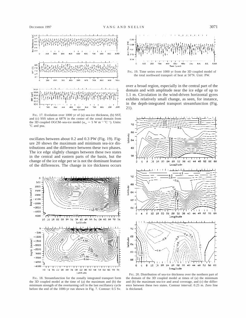
north of 528N for the standard run, using kiw 5 5 Wm22 8C21. The model oscillates when ice interaction isincluded. Figure 17 shows a 1000-yr evolution of sea-ice thickness, SST, and SSS taken at 688N in midbasin.The period of the oscillation is about 25 yr. The mech-anism for this oscillation is essentially the same as thatexplained in the previous section. A careful examinationshows that the sea-ice variation lags that of SST by one-quarter of a cycle, while the peak of sea-ice variationleads the trough of SSS variation by a quarter cycle.This phase relation is very similar to that found in theYN93’s coupled ocean–ice oscillation. The overturningcirculation also oscillates with the same frequency. Fig-ure 18 shows the overturning cell at maximum and min-imum strength during one oscillatory cycle. The THCvaries from about 13 to about 7.5 Sv in this run. Becauseof this oscillation, the northward transport of heat alsooscillates. The total northward transport of heat at 508N


FIG. 17. Evolution over 1000 yr of (a) sea-ice thickness, (b) SST,and (c) SSS taken at 688N in the center of the zonal domain fromthe 3D coupled OGCM–sea-ice model (kiw 5 5 W m22 8C21). Units:8C and psu.

FIG. 19. Time series over 1000 yr from the 3D coupled model ofthe total northward transport of heat at 508N. Unit: PW.

FIG. 20. Distribution of sea-ice thickness over the northern part ofthe domain of the 3D coupled model at times of (a) the minimumand (b) the maximum sea-ice and areal coverage, and (c) the differ-ence between these two states. Contour interval: 0.25 m. Zero lineis thickened.

FIG. 18. Streamfunction for the zonally integrated transport formthe 3D coupled model at the time of (a) the maximum and (b) theminimum strength of the overturning cell in the last oscillatory cyclebefore the end of the 1000-yr run shown in Fig. 7. Contour: 0.5 Sv.

oscillates between about 0.2 and 0.3 PW (Fig. 19). Fig-ure 20 shows the maximum and minimum sea-ice dis-tributions and the difference between these two phases.The ice edge slightly changes between these two statesin the central and eastern parts of the basin, but thechange of the ice edge per se is not the dominant featureof the differences. The change in ice thickness occurs

over a broad region, especially in the central part of thedomain and with amplitude near the ice edge of up to1.1 m. Circulation in the wind-driven horizontal gyresexhibits relatively small change, as seen, for instance,in the depth-integrated transport streamfunction (Fig.21).


FIG. 21. The barotropic transport streamfunction in the 3D model.Unit: Sv.

FIG. 22. Snapshots of anomalous zonally averaged temperature from the 3D model distributionat (a) a warm state and (b) a cold state. Both states were taken during the last oscillatory cyclebefore the end of the 1000-yr run shown in Fig. 7. Contour interval: 0.058C.

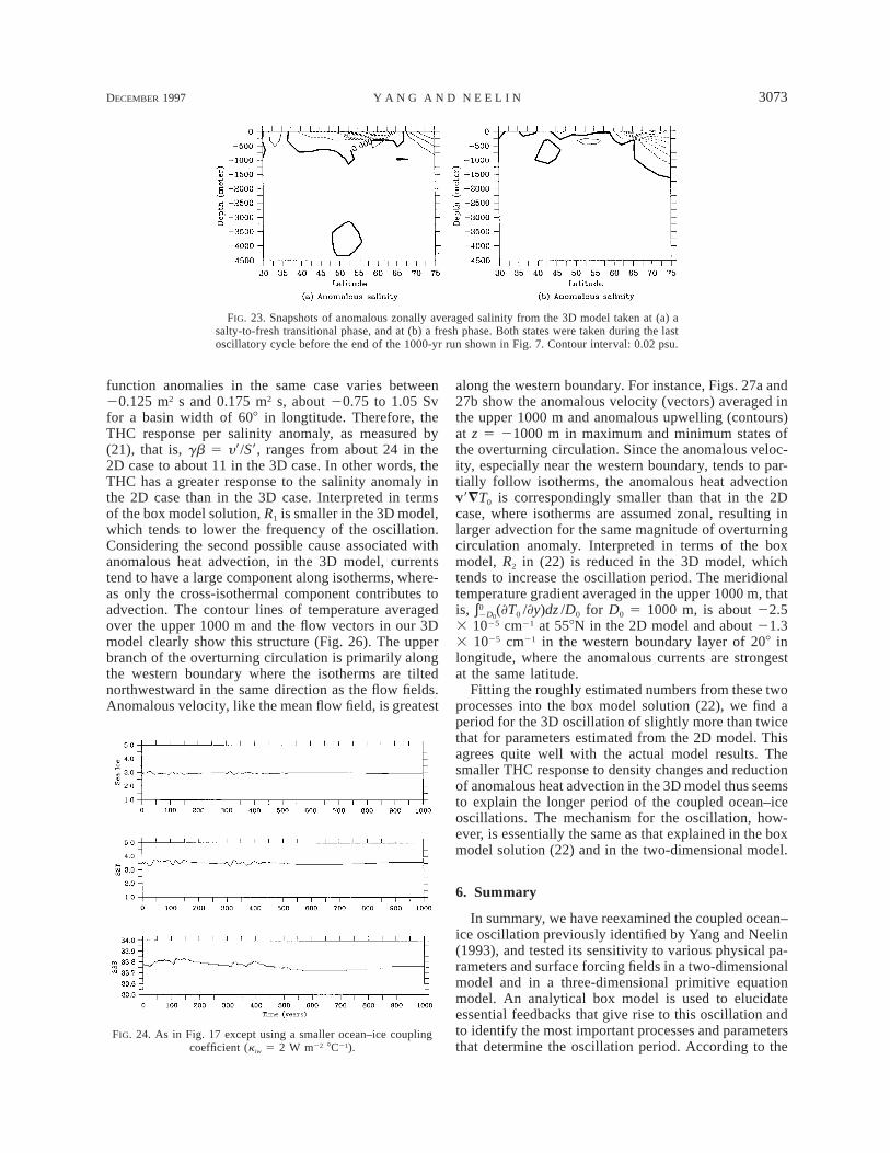
The anomalous temperature distributions at warm(Fig. 22a) and cold (Fig. 22b) phases show that themaximum variations occur in the upper 1000 m over aregion about 208 latitude wide near the northern bound-ary. The salinity variations (Fig. 23) are likewise trappedin the upper 1000 m. They are more localized near thenorthern boundary in the ice region during fresh or saltyphases. During transition phases, additional salinityanomalies due to advection may be noted south of theice region.

The oscillation characteristics are consistent with theYN93 results. It is worth underlining that this oscillationis not the same as the heat–ice oscillation identified byWelander (1977) and recently examined by Zhang et al.(1995) in a 3D model. The heat–ice oscillation discussedin those two papers arises due to change of sea-ice extentand the associated change in thermal insulation effectand salinity does not play a significant role. Welander’s(1977) model did not include salinity and a similar fresh-water conceptual model was used by Zhang et al. (1995)to explain their model oscillations. In contrast, salinityplays a leading role in our model oscillation. Turning

off the salinity feedback from sea-ice melting and freez-ing stabilizes the model state and the oscillation dis-appears. In addition, the heat–ice oscillation of Welan-der (1977) and Zhang et al. (1995) should become morerobust when a smaller ocean–ice heat flux coefficientkiw is used since it amplifies the effect of thermal in-sulation. As shown in the following sensitivity test, os-cillations are damped when a smaller kiw is used in ourmodel.

Figures 24 and 25 show the sensitivity to the ocean–ice coupling coefficient, kiw. When the value of thisparameter is reduced from 5 to 2 W m22 8C21, the modelbecomes stable and no oscillation is generated (Fig. 24).The model produces chaotic variations when kiw is in-creased to 30 W m22 8C21 (Fig. 25). These are quali-tatively consistent with the two-dimensional model’s re-sults shown in section 4a. Additional experiments alsoshow that the model stabilizes in a more diffusive re-gime.

The most significant difference between the oscilla-tion in the two dimensional model and the oscillationin the three-dimensional model is that the period is con-siderably longer in the latter. Since the same sea-icemodel is used in both 2D and 3D cases, the differencesare due to the model representations of oceanic pro-cesses. As explained in the simple box model (22), theoscillation period is controlled by a number of pro-cesses, labeled R1, R2, R3, and R4. Both R4, which mea-sures the ocean–ice coupling and the surface Newtoniandamping on SST in ice-covered areas, and R3, whichmeasures the freezing/melting rate in response to an SSTanomaly, remain unchanged since the same ice modelis used. The cause for the longer oscillation period inthe 3D model is most likely due either to the differencein the circulation response to density anomalies, that is,R1 in (22), or to the differences in anomalous heat ad-vection [R2 in (22)] when the flow has a three-dimen-sional structure. In the 3D case, the change of salinity,as shown in Fig. 17c, is about 0.5 psu, and the corre-sponding change of the THC is about 5.5 Sv (Fig. 18).However, in the 2D case, the surface salinity oscillateswithin 0.075 psu (dashed line in Fig. 5). The stream-


FIG. 23. Snapshots of anomalous zonally averaged salinity from the 3D model taken at (a) asalty-to-fresh transitional phase, and at (b) a fresh phase. Both states were taken during the lastoscillatory cycle before the end of the 1000-yr run shown in Fig. 7. Contour interval: 0.02 psu.

FIG. 24. As in Fig. 17 except using a smaller ocean–ice couplingcoefficient (kiw 5 2 W m22 8C21).

function anomalies in the same case varies between20.125 m2 s and 0.175 m2 s, about 20.75 to 1.05 Svfor a basin width of 608 in longtitude. Therefore, theTHC response per salinity anomaly, as measured by(21), that is, gb 5 y9/S9, ranges from about 24 in the2D case to about 11 in the 3D case. In other words, theTHC has a greater response to the salinity anomaly inthe 2D case than in the 3D case. Interpreted in termsof the box model solution, R1 is smaller in the 3D model,which tends to lower the frequency of the oscillation.Considering the second possible cause associated withanomalous heat advection, in the 3D model, currentstend to have a large component along isotherms, where-as only the cross-isothermal component contributes toadvection. The contour lines of temperature averagedover the upper 1000 m and the flow vectors in our 3Dmodel clearly show this structure (Fig. 26). The upperbranch of the overturning circulation is primarily alongthe western boundary where the isotherms are tiltednorthwestward in the same direction as the flow fields.Anomalous velocity, like the mean flow field, is greatest

along the western boundary. For instance, Figs. 27a and27b show the anomalous velocity (vectors) averaged inthe upper 1000 m and anomalous upwelling (contours)at z 5 21000 m in maximum and minimum states ofthe overturning circulation. Since the anomalous veloc-ity, especially near the western boundary, tends to par-tially follow isotherms, the anomalous heat advectionv9=T0 is correspondingly smaller than that in the 2Dcase, where isotherms are assumed zonal, resulting inlarger advection for the same magnitude of overturningcirculation anomaly. Interpreted in terms of the boxmodel, R2 in (22) is reduced in the 3D model, whichtends to increase the oscillation period. The meridionaltemperature gradient averaged in the upper 1000 m, thatis, (]T0 /]y)dz /D0 for D0 5 1000 m, is about 22.50∫2D0

3 1025 cm21 at 558N in the 2D model and about 21.33 1025 cm21 in the western boundary layer of 208 inlongitude, where the anomalous currents are strongestat the same latitude.

Fitting the roughly estimated numbers from these twoprocesses into the box model solution (22), we find aperiod for the 3D oscillation of slightly more than twicethat for parameters estimated from the 2D model. Thisagrees quite well with the actual model results. Thesmaller THC response to density changes and reductionof anomalous heat advection in the 3D model thus seemsto explain the longer period of the coupled ocean–iceoscillations. The mechanism for the oscillation, how-ever, is essentially the same as that explained in the boxmodel solution (22) and in the two-dimensional model.

6. Summary

In summary, we have reexamined the coupled ocean–ice oscillation previously identified by Yang and Neelin(1993), and tested its sensitivity to various physical pa-rameters and surface forcing fields in a two-dimensionalmodel and in a three-dimensional primitive equationmodel. An analytical box model is used to elucidateessential feedbacks that give rise to this oscillation andto identify the most important processes and parametersthat determine the oscillation period. According to the


FIG. 25. As in Fig. 17 except using a greater ocean–ice coupling coefficient (kiw 5 30 W m22

8C21).

FIG. 26. Mean temperature contours and mean current fields (vec-tors) from the 3D model, both averaged in the upper 1000 m, for thecase shown in Fig. 18.

box model, the oscillation mechanism can be summa-rized (dropping some quantitatively important but no-nessential terms) by

frequency 5 [R1R2R3]1/2,

where

R 5 (THC velocity anomaly per salinity anomaly),1

R 5 (temperature gradient), and2

R 5 (rate of freshening by ice melt per SST anomaly).3

A salinity increase in the sinking region causes an in-crease in the surface velocity of the overturning cir-culation (R1; m s21 psu21). This advects warm temper-atures into the sinking region due to the temperaturegradient between the sinking region and the regionwhere the inflow comes from (R2; K m21). The warmingmelts ice, which gives a freshening tendency that leadsto the opposite phase of the cycle (R3; psu s21 K 21).This makes clear that the oscillation timescale is trulya characteristic of the coupled system, depending on acombination of factors from both the ocean and the ice.None of these factors is a timescale characteristic of theindividual systems.

When coupled with a linearized version of the sea-ice model, the 2D model becomes stable in the weakcoupling regime and generates self-sustained oscilla-tions as the ocean–ice coupling coefficient increases.


FIG. 27. Anomalous velocities (vector) averaged over the upper1000 m and upwelling field (contour lines in m day21) at the depthof 1000 m (a) at a state of maximum THC overturning and (b) at astate of minimum THC overturning.

The oscillation period is quite insensitive to the intensityof this coupling. The model becomes more stable whengreater diffusivity is used. In the stable parameter re-gime, interdecadal oscillations can be sustained by sto-chastic forcing. The coupled instability is sensitive tothe amplitude of THC feedbacks, as determined by vis-cosities AV and AH in the 2D model equation (1) or gin the box model solution (22). The model becomesmore unstable and its oscillation period shortens towardgreater THC feedback. We have also examined the caseof using a nonlinear sea-ice model. The model behavessimilarly as in the linear case when a small or an in-termediate ocean–ice coupling coefficient is used, butbecomes stable in high coupling regime. This can beexplained in terms of the change of the effective damp-ing on sea ice associated with the change of sea-icethickness. The period of the oscillation in the nonlinearsea-ice case is also robust. Chaotic behavior of the os-cillation was found in some parametric regimes. Inser-tion of a sponge layer in the 2D model is used to showthat the essential variability is rather localized and thusa regional model can be used for studies with the 3Dmodel. An additional experiment was run to show thatthe oscillation is also robust when a two-cell THC cli-matology is used.

Results from using the GFDL OGCM MOM coupledwith the nonlinear sea-ice model are also presented. This3D model also produces an interdecadal coupled ocean–ice oscillation. The mechanism is the same as that iden-tified in the 2D model and explained in the box model.The major difference is that the period of oscillationbecomes considerably longer, roughly 26 yr. The longerperiod is mainly due to a smaller THC response to sa-linity anomalies and to smaller poleward heat advectionby anomalous flow fields in the 3D model compared tothe 2D model. The box model explains the reduction infrequency as a reduction in both R1 and R2 (above). Interms of making a case for this oscillation mechanismbeing likely to occur in the observed ocean–ice system,some caveats on the 3D model are the lack of realisticgeography, the relatively coarse resolution, the lack ofice advection, and the simple atmospheric boundaryconditions. Nonetheless, the robustness of the oscilla-tion in the two dimensional THC–ice model where itwas first predicted, and the new demonstration of itsexistence in the three-dimensional model are encour-aging. It suggests that this physical mechanism is worthseeking in data and in coupled ocean–atmosphere–iceGCMs.

Acknowledgments. This work was supported byNOAA Atlantic Climate Change Program GrantNA56GP0209 (JY), National Science FoundationGrants ATM-9158294 and ATM-9521389 (JDN andJY), a grant from the National Institute for Global En-vironmental Change (JDN and JY), and a Mellon In-dependent Study Award from the Woods Hole Ocean-ographic Institution (JY). We benefited from conver-


sations with Drs. R. X. Huang, J. Marotzke, P. Stone,and J. Walsh. We thank Dr. A. Weaver and Mr. E. Wiebefor helpful comments, and welcome the news that thisoscillation occurs in their ocean–atmosphere model (A.Weaver and E. Wiebe 1996, personal communication).

REFERENCES

Bryan, F. O., 1986: High-latitude salinity effects and interhemisphericthermohaline circulation. Nature, 323, 301–304.

Bryan, K., 1969: A numerical method for the study of the circulationof the world ocean. J. Comput. Phys., 4, 347–376.

Chen, F., and M. Ghil, 1995: Interdecadal variability of the ther-mohaline circulation and high-latitude surface fluxes. J. Phys.Oceanogr., 25, 2547–2568.

Delworth, T., S. Manabe, and R. J. Stouffer, 1993: Interdecadal vari-ations of the thermohaline circulation in a coupled ocean–at-mosphere model. J. Climate, 6, 1993–2011.

Deser, C., and M. L. Blackmon, 1993: Surface climate variations overthe North Atlantic Ocean during winter: 1900–1989. J. Climate,6, 1743–1753.

Dickson, R. R., J. Meincke, S. A. Malmberg, and A. J. Lee, 1988:The ‘‘great salinity anomaly’’ in the northern North Atlantic1968–1982. Progress in Oceanography, Vol. 20, PergamonPress, 103–151.

Ghil, M., and R. Vautard, 1991: Interdecadal oscillations and thewarming trend in global temperature time series. Nature, 350,324–327.

Gill, A. E., 1982: Atmosphere–Ocean Dynamics. Academic Press,662 pp.

Haney, R. L., 1971: Surface thermal boundary conditions for oceangeneral circulation models. J. Phys. Oceanogr., 1, 241–248.

Hasselmann, K., 1976: Stochastic climate models. Tellus, 28, 473–485.

Houssais, M. N., and W. D. Hibler III, 1993: Importance of convectivemixing in seasonal ice margin simulations. J. Geophys. Res., 98,16 427–16 448.

Huang, R. X., 1993: Real freshwater flux as a natural boundary con-dition for salinity balance and thermohaline circulation forcedby evaporation and precipitation. J. Phys. Oceanogr., 23, 2428–2446., 1994: Thermohaline circulation: Energetics and variability ina single hemisphere basin model. J. Geophys. Res., 99, 12 471–12 485.

Kushnir, Y., 1994: Interdecadal variations in North Atlantic sea sur-face temperature and associated atmospheric conditions. J. Cli-mate, 7, 141–157.

Levitus, S., 1982. Climatological atlas of the world ocean. NOAAProf. Paper 13, U.S. Government Printing Office, Washington,DC, 173 pp. [Available from U.S. Government Printing Office,Washington, DC 20402.]

Marotzke, J., P. Welander, and J. Willebrand, 1988: Instability andmultiple steady states in a meridional plane model of the ther-mohaline circulation. Tellus, 40A, 162–172.

Maykut, G. A., and N. Untersteiner, 1971: Some results from a time-

dependent, thermodynamic model of sea-ice. J. Geophys. Res.,76, 1550–1575.

Mikolajewicz, U., and E. Maier-Reimer, 1990: Internal secular vari-ability in an ocean general circulation model. Climate Dyn., 4,145–156.

Mysak, L. A., D. K. Manak, and R. F. Marsden, 1990: Sea-ice anom-alies observed in the Greenland and Labrador Seas during 1901–1984 and their relation to an interdecadal Arctic climate cycle.Climate Dyn., 5, 111–133.

Nayfeh, A. H., and B. Balachandran, 1995: Applied Nonlinear Dy-namics, Analytical, Computational, and Experimental Methods.John Wiley and Sons, 685 pp.

Oort, A., 1983: Global atmospheric circulation statistics 1958–1973.NOAA Prof. Paper 14, U.S. Government Printing Office, Wash-ington, DC, 174 pp. [Available from U.S. Government PrintingOffice, Washington, DC 20402.]

Pacanowski, R. C., K. Dixon, and A. Rosati, 1993: The GFDL mod-ular ocean model users guide. GFDL Ocean Group Tech. Rep.,232 pp. [Available from U.S. Government Printing Office, Wash-ington, DC 20402.]

Strogatz, S. H., 1994: Nonlinear Dynamics and Chaos. Addison-Wesley Publishing, 498 pp.

Thorndike, A. S., 1992: A toy model of sea ice growth. Modelingthe Earth System, D. Ojima, Ed., UCAR/Office for Interdisci-plinary Earth Studies, 225–238.

Walsh, J. E., and W. L. Chapman, 1990: Arctic contribution to upper-ocean variability in the North Atlantic J. Climate, 3, 1462–1473.

Weaver, A. J., E. S. Sarachik, and J. Marotzke, 1991: Freshwater fluxforcing of decadal and interdecadal oceanic variability. Nature,353, 836–838.

Welander, P., 1977: Thermal oscillations in a fluid heated from belowand cooled to freezing from above. Dyn. Atmos. Oceans, 1, 215–223., 1986: Thermohaline effects in the ocean circulation and relatedsimple models. Large-Scale Transport Processes in Oceans andAtmosphere, J. Willebrand and D. L. T. Anderson, Eds., D. Rei-del, 163–200.

Willmott, A. J., and L. A. Mysak, 1989: A simple steady-state coupledice–ocean model, with application to the Greenland–NorwegianSea. J. Phys. Oceanogr., 19, 501–518.

Winton, M., and E. S. Sarachik, 1993: Thermohaline oscillation in-duced by strong steady state forcing of ocean general circulationmodels. J. Phys. Oceanogr., 23, 1389–1410.

Yang, J., and J. D. Neelin, 1993: Sea-ice interaction with the ther-mohaline circulation. Geophys. Res. Lett., 20, 217–220., and S. Honjo, 1996: Modeling the near-freezing dichothermallayer of the Sea of Okhotsk. J. Geophys. Res., 101 (C7), 16 421–16 433., and R. X. Huang, 1996: The annual cycle and its role in gen-erating interannual and decadal variations at high-latitudeoceans. Geophys. Res. Lett., 23, 269–272., and J. D. Neelin, 1996: Sea-ice interaction and the stability ofthe thermohaline circulation in response to long-term climatechange. Atmos.–Ocean, in press.

Zhang, S., C. A. Lin, and R. J. Greatbatch, 1995: A decadal oscillationdue to the coupling between an ocean circulation model and athermodynamic sea-ice model. J. Mar. Res., 53, 79–106.

Documents

Decadal Variability in Coupled Sea-Ice–Thermohaline ...research.atmos.ucla.edu/csi/REF/pdfs/newice.pdftem. Since the THC involves long timescales, it is po-tentially a rich source