Embed Size (px)
Citation preview
3596 VOLUME 32J O U R N A L O F P H Y S I C A L O C E A N O G R A P H Y
q 2002 American Meteorological Society
Japan Sea Thermohaline Structure and Circulation.Part III: Autocorrelation Functions
PETER C. CHU
Naval Ocean Analysis and Prediction Laboratory, Department of Oceanography, Naval Postgraduate School, Monterey, California
WANG GUIHUA
Laboratory of Ocean Dynamic Processes and Satellite Oceanography, Second Institute of Oceanography,State Oceanic Administration, Hangzhou, China
YUCHUN CHEN
Cold and Arid Regions Environmental and Engineering, Research Institute, Lanzhou, China
(Manuscript received 29 January 2001, in final form 17 June 2002)
ABSTRACT
The autocorrelation functions of temperature and salinity in the three basins (Ulleung, Japan, and YamatoBasins) of the Japan/East Sea are computed using the U.S. Navy’s Master Oceanographic Observational Datasetfor 1930–97. After quality control the dataset consists of 93 810 temperature and 50 349 salinity profiles. Thedecorrelation scales of both temperature and salinity were obtained through fitting the autocorrelation functioninto the Gaussian function. The signal-to-noise ratios of temperature and salinity for the three basins are usuallylarger than 2. The signal-to-noise ratio of temperature is greater in summer than in winter. There is more noisein salinity than in temperature. This might be caused by fewer salinity than temperature observations. Theautocorrelation functions of temperature for the three basins have evident seasonal variability at the surface:less spatial variability in the summer than in the winter. The temporal (spatial) decorrelation scale is shorter(longer) in the summer than in the winter. Such a strong seasonal variability at the surface may be caused bythe seasonal variability of the net surface heat flux. The autocorrelation functions of salinity have weaker seasonalvariability than those of the temperature field. The temporal and horizontal decorrelation scales obtained in thisstudy are useful for designing an optimal observational network.
1. Introduction
The Japan/East Sea, hereafter referred to as JES, isa semienclosed ocean basin covering an area of 106 km2
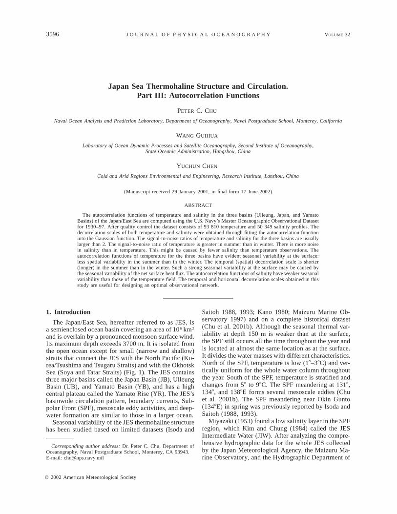
and is overlain by a pronounced monsoon surface wind.Its maximum depth exceeds 3700 m. It is isolated fromthe open ocean except for small (narrow and shallow)straits that connect the JES with the North Pacific (Ko-rea/Tsushima and Tsugaru Straits) and with the OkhotskSea (Soya and Tatar Straits) (Fig. 1). The JES containsthree major basins called the Japan Basin (JB), UlleungBasin (UB), and Yamato Basin (YB), and has a highcentral plateau called the Yamato Rise (YR). The JES’sbasinwide circulation pattern, boundary currents, Sub-polar Front (SPF), mesoscale eddy activities, and deep-water formation are similar to those in a larger ocean.
Seasonal variability of the JES thermohaline structurehas been studied based on limited datasets (Isoda and
Corresponding author address: Dr. Peter C. Chu, Department ofOceanography, Naval Postgraduate School, Monterey, CA 93943.E-mail: [email protected]
Saitoh 1988, 1993; Kano 1980; Maizuru Marine Ob-servatory 1997) and on a complete historical dataset(Chu et al. 2001b). Although the seasonal thermal var-iability at depth 150 m is weaker than at the surface,the SPF still occurs all the time throughout the year andis located at almost the same location as at the surface.It divides the water masses with different characteristics.North of the SPF, temperature is low (18–38C) and ver-tically uniform for the whole water column throughoutthe year. South of the SPF, temperature is stratified andchanges from 58 to 98C. The SPF meandering at 1318,1348, and 1388E forms several mesoscale eddies (Chuet al. 2001b). The SPF meandering near Okin Gunto(1348E) in spring was previously reported by Isoda andSaitoh (1988, 1993).
Miyazaki (1953) found a low salinity layer in the SPFregion, which Kim and Chung (1984) called the JESIntermediate Water (JIW). After analyzing the compre-hensive hydrographic data for the whole JES collectedby the Japan Meteorological Agency, the Maizuru Ma-rine Observatory, and the Hydrographic Department of
DECEMBER 2002 3597C H U E T A L .
FIG. 1. Geography and isobaths showing the bottom topography of the Japan/East Sea (JES).Nonuniform contour intervals are used.
the Japan Maritime Safety Agency, Senjyu (1999)shows the existence of a salinity minimum (SMIN) layer(i.e., JIW) between the surface water and the JES ‘‘Prop-er Water.’’
With the hydrographic data collected from an inter-national program, Circulation Research of the EastAsian Marginal Seas (CREAMS) 1993–96, Kim andKim (1999) found high salinity water with high oxygenin the eastern JB (i.e., north of SPF) which they calledthe ‘‘High Salinity Intermediate Water’’ (HSIW). Kimet al. (1999) found that the upper warm water is mostsaline in the UB and YB, that salinity of the intermediatewater is the highest in the eastern JB, and that the deepcold water has highest salinity in the JB. This indicatesthat the three basins have different thermohaline struc-tures.
In the first two parts of this paper, Chu et al. (2001a,b)reported the seasonal variation of the thermohalinestructure and calculated currents from the navy’s un-classified Generalized Digital Environmental Model(GDEM; Teague et al. 1990) temperature and salinitydata on a 109 3 109 grid. The GDEM for the JES is
built on historical profiles. A three-dimensional estimateof the absolute geostrophic velocity field was obtainedfrom the GDEM temperature and salinity fields usingthe P-vector method (Chu 1995). The climatologicalmean and seasonal variabilities of the thermohalinestructure and the calculated currents such as the SPF,the Tsushima Warm Current (TWC), and its bifurcationwere identified.
The thermohaline variabilities of these basins can bedetermined through computing the autocorrelation func-tions (ACF) of temperature and salinity at depth (z)using historical data. The ACF for temperature or sa-linity is given by (Chu et al. 1997b)
L1h(l, z) 5 c9(l , z)c9(l 1 l, z) dl , (1)E 0 0 02s
where c9 is the anomaly (relative to the climatologicalmean values), l0 denotes the independent space/timevectors defining the location of points in a samplingspace L, l is the space/time lag, and s2 the variance; his computed by paring the anomalies into bins depend-
3598 VOLUME 32J O U R N A L O F P H Y S I C A L O C E A N O G R A P H Y
ing upon their separation in space/time, l. The valuesof h are obtained from calculating the correlation co-efficient for all the anomaly pairs in each bin constructedfor the combination of different lags.
Temporal and horizontal decorrelation scales of theJES thermohaline fields have not been calculated before.The U.S. Navy’s Master Oceanographic ObservationalData Set (MOODS) contains (93 810) temperature and(50 349) salinity profiles (unclassified) for JES during1930–97 (Fig. 2). This provides the opportunity to com-pute the thermohaline ACFs.
The outline of this paper is as follows: Section 2 isbackground on the JES current systems and the divisionof data on the basis of the hydrographic properties. Sec-tion 3 discusses the irregularity of the navy’s MOODSdata. Sections 4 and 5 depict space/time sorting andACF calculation. The seasonal variabilities of the de-correlation scales and their application are discussed insections 6 and 7. In section 8 we present our conclu-sions.
2. JES current systems and geographic regions
The JES has subtropical and subpolar circulationsseparated by SPF. Most of the nearly homogeneous wa-ter in the deep part of the basin is called the ‘‘JapanSea Proper Water’’ (Moriyasu 1972) and is of low tem-perature and low salinity. Above the Proper Water, theTWC, dominating the surface layer, flows in from theEast China Sea through the Korea/Tsushima Strait andcarries warm, salty Kuroshio water from the south. TheLiman Cold Current (LC) carries cold fresh surface wa-ter from the north and northeast. The properties of thissurface water are generally believed to be determinedby the strong wintertime cooling coupled with fresh-water input from the Amur River and the melting seaice in Tatar Strait (Martin and Kawase 1998). The LCflows southward along the Russian coast, beginning ata latitude slightly north of Soya Strait, terminating offVladivostok, and becoming the North Korean Cold Cur-rent (NKCC) after reaching the North Korean coast(Yoon 1982).
The TWC separates into two branches, which flowthrough the western and eastern channels of the Korea/Tsushima Strait (Kawabe 1982a,b; Hase et al. 1999).The flow through the eastern channel closely followsthe Japanese coast and is called the ‘‘Nearshore Branch’’(Yoon 1982) or the first branch of TWC (FBTWC: Haseet al. 1999). The flow through the western channel iscalled the East Korean Warm Current (EKWC), whichclosely follows the Korean coast until it separates near378N into two subbranches. The western subbranchmoves northward and forms a cyclonic eddy over UBoff the eastern Korean coast. The eastern subbranchflows eastward to the western coast of Hokkaido Island,and becomes the second branch of the TWC (SBTWC;Hong and Cho 1983). However, the SBTWC may notexist all year and cannot always be found around the
shelf because its path is influenced by the developmentof eddies (Hase et al. 1999).
The NKCC meets the EKWC at about 388N. Afterseparation from the coast, the NKCC and the EKWCconverge and form a strong front that stretches in thezonal direction across the basin. The NKCC makes acyclonic recirculation gyre in the north but most of theEKWC flows out through Tsugaru and Soya Straits (Uda1934). The formation of NKCC and separation ofEKWC are due to local forcing by wind and buoyancyflux (Seung 1994). Large meanders develop along thefront and are associated with warm and cool eddies.
The ACF depends on water mass properties. Differentthermohaline characteristics are found north and southof the SPF, which is located about 408N. The upperwarm water is more saline south of the SPF, while theintermediate and deep cold water is more saline northof the SPF (Kim et al. 1999). South of the SPF, differentthermohaline characteristics are found west and east of1328E. The southwestern JES west of 1328E is the up-stream region of the JIW (Senjyu 1999). The lowestsalinity and the highest oxygen concentration are foundin the 388–408N areas west of 1328E. The JIW takestwo flow paths: an eastward flow along the SPF and asouthward flow parallel with the Korean coast in theregion west of 1328E. The circulation pattern west andeast of 1328E is also different: dual eddies (cyclone inthe north and anticyclone in the south) occur west of1328E, while there are two branches of TWC east of1328E (Senjyu 1999). Thus, 408N latitude and 1328Elongitude are used here to divide the JES into three parts(Fig. 1) with different water mass characteristics.
The Korean/Tsushima Strait is a major continentalshelf with many observations. However, the water masson the shelf, largely affected by the atmospheric forcing,is different from the water mass of the JES basin andtherefore should be deleted for the computation. Twoapproaches are used: (i) a southern boundary is set upat 35.58N and (ii) profiles in water depth shallower than100 m are excluded.
Thus, the ACF is separately computed for the threeparts of JES: north of 408N (represented by JB), westof 1328E between 35.58 and 408N (represented by UB),and east of 1328E between 35.58 and 408N (representedby YB). The partition into JB, UB, and YB here is basedon water mass characteristics and may not be exactlythe same as the geographic definitions.
3. Irregularity of the MOODS
To investigate the seasonal variation of the temporaland spatial scales for the three basins, the MOODS wasbinned into four seasons. The seasons were defined ac-cording to the convention of the Naval OceanographicOffice for the JES: January–March constitute winter;April–June, spring; July–September, summer; and Oc-tober–December, fall.
The main limitation of the dataset is its irregular dis-
DECEMBER 2002 3599C H U E T A L .
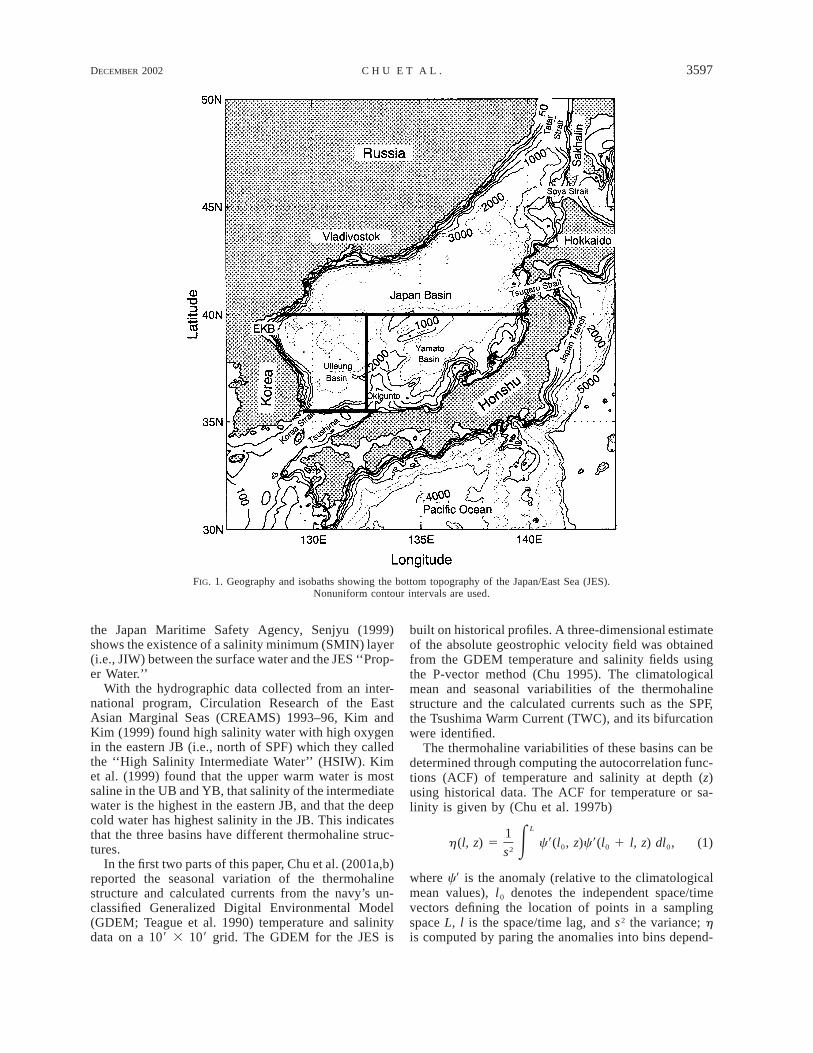
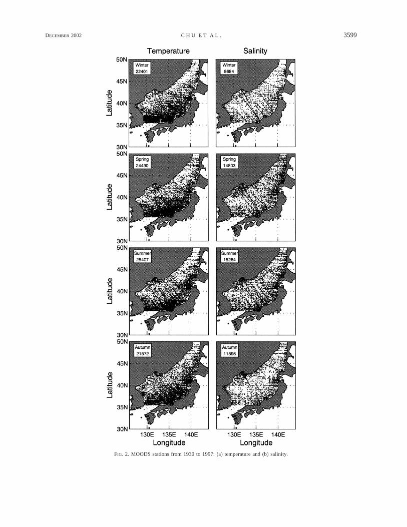
FIG. 2. MOODS stations from 1930 to 1997: (a) temperature and (b) salinity.
3600 VOLUME 32J O U R N A L O F P H Y S I C A L O C E A N O G R A P H Y
TABLE 1. Number of temperature profiles in the database for eachbasin and each season.
JB UB YB
WinterSpringSummerFall
5203770481637012
4612416047394503
12 58612 56612 50510 057
tribution in time and space. Certain periods and areasare oversampled while others lack enough observationsto gain any meaningful insights (Chu et al. 1997a). Thevertical extent of the observations and data quality arealso highly variable. The eastern coastal region of NorthKorea is a data sparse area. Horizontal (Fig. 2) andtemporal irregularities along with the lack of data incertain regions must be carefully weighted in order toavoid statistically induced variability. Analysis wasdone on a mean seasonal basis using the data for allyears.
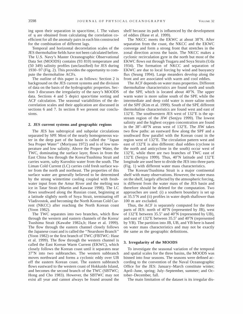
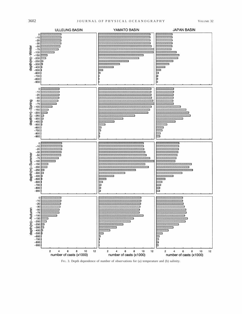
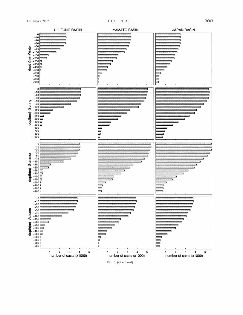
The number of temperature and salinity (Fig. 2) ob-servations differs drastically from basin to basin (Tables1 and 2). The YB has the most temperature observationsin the four seasons. However, JB has the most salinityobservations in spring and summer. Salinity profiles arefewer than temperature profiles in all seasons and forall basins. The number of observations vary with depth(Fig. 3). Many temperature and salinity samples werecollected above depth 100 m. The vertical variation ofsampling changes from basin to basin. For example, inUB, the number of T, S samples decreases rapidly withdepth below 75 m. In JB, the number of temperaturesamples reaches a maximum at depth 200–250 m inspring and summer.
4. ACF computation
The three basins (JB, UB, YB) may be treated asquasi-isolated systems. Therefore, it is assumed that theACF for each basin depends only on the distance be-tween two locations in order to reduce the number ofbins. Without this assumption, the number of bins isvery large—for example, 27 000 if each of the temporaland spatial (x and y) lags has 30 bins.
For each observation at depth z (c represents T,(z)c o
S), the closest grid point climatological value (fromGDEM) is found and the anomaly, 5 2
(z)(z) (z)c c 9 cl o o
is computed. GDEM is the navy’s global climato-(z)
c l
logical monthly mean temperature and salinity dataset(0.58 3 0.58) from the surface to bottom. The currentversion of the GDEM climatology was based on thenavy’s MOODS (Teague et al. 1991).
The ACF is calculated (see appendix A) for eachspatial lag bin (with increment Dr 5 10 km) and tem-poral lag bin (with increment Dt 5 1 day). For eachindividual anomaly, , all the other data points,(z)c 9o
are sorted into different spatial and temporal bins(z)c 9o
within the four seasons. If the lags between and(z)c 9o
(called a data pair) are within Dr0 (5 km) and Dt0(z)c 9o
(0.5 day), the corresponding pair is placed into bin (0,0). If the horizontal lag is between mDr 2 Dr0 and mDr1 Dr0, and the temporal lag between nDt 2 Dt0 andnDt 1 Dt0, the pair is placed into the bin (m, n).
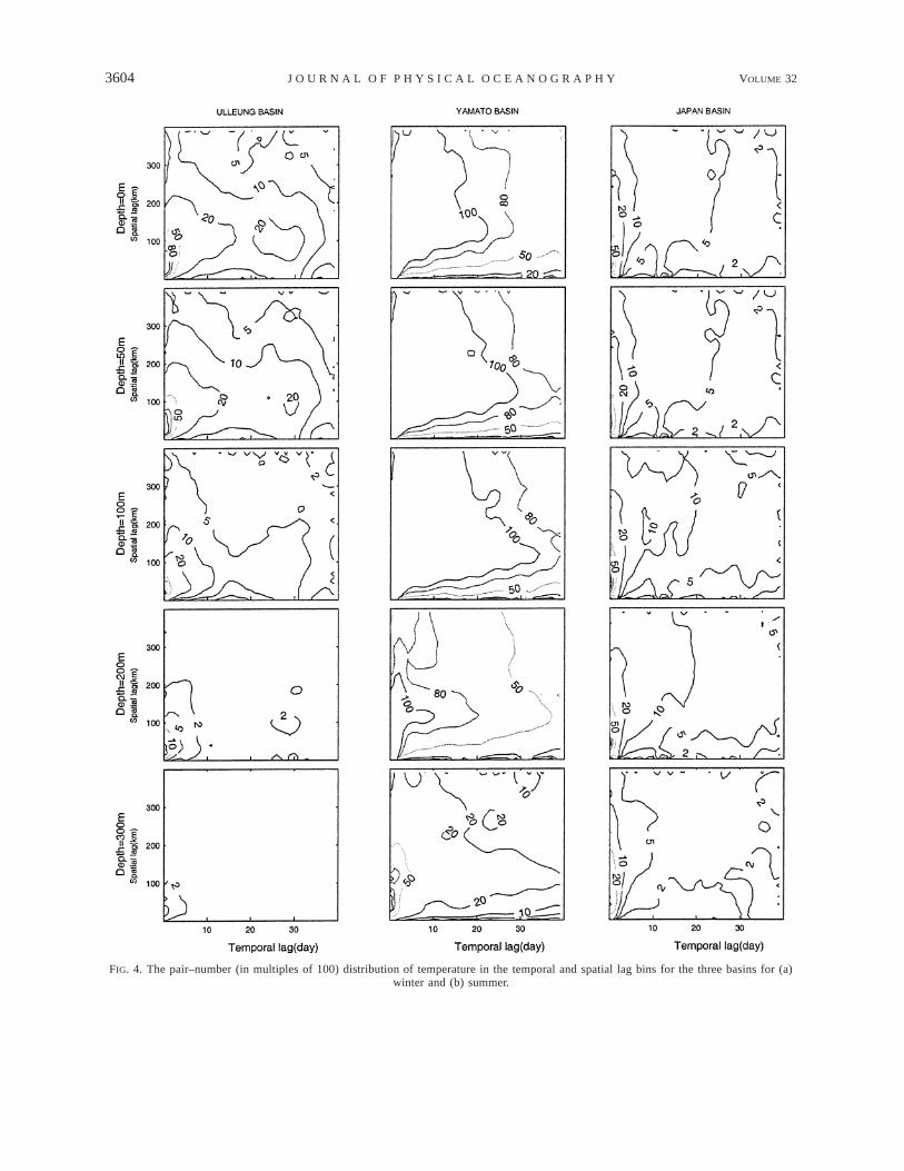
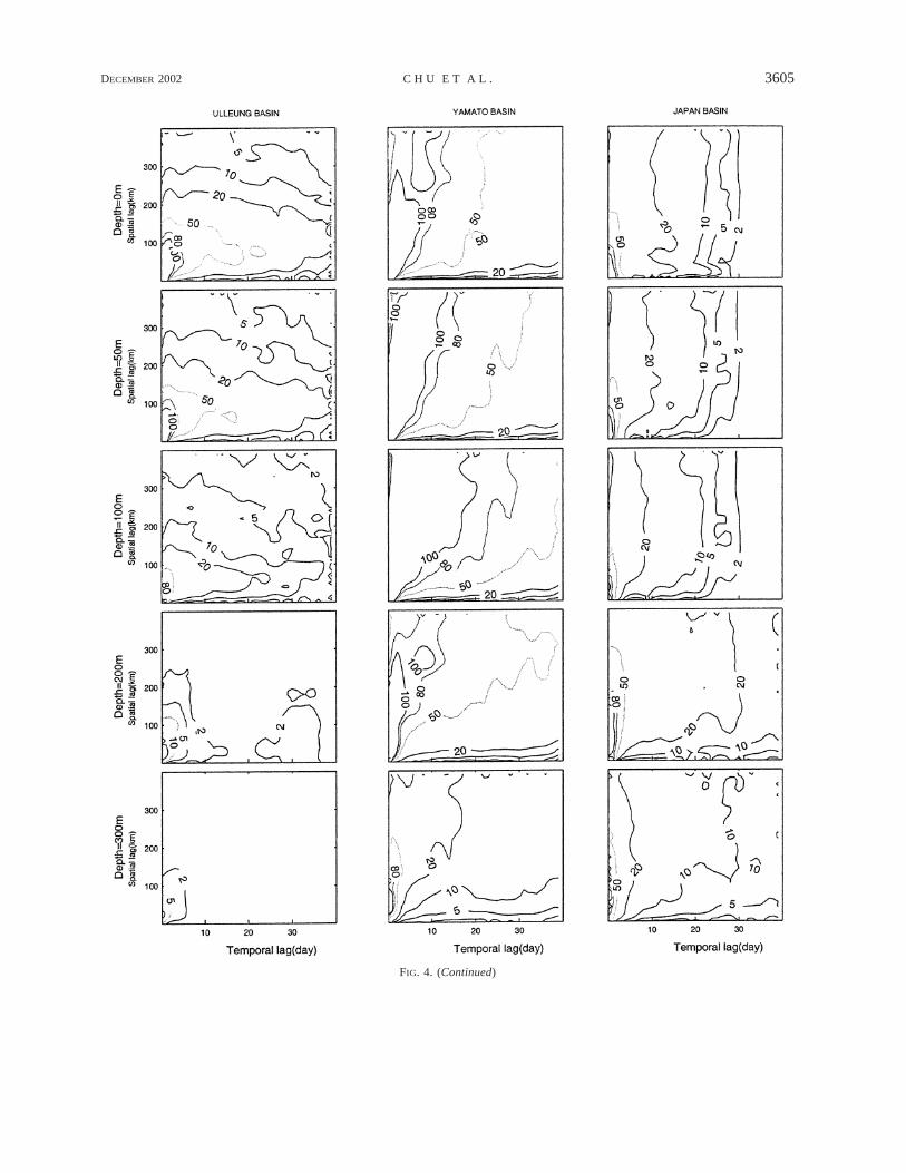
The pair–number distributions, P(m, n), of tempera-ture and salinity for winter and summer are illustratedin Figs. 4 and 5. We see uneven distribution in thetemporal and spatial bins, however, the seasonal vari-ation of P(m, n) is weaker than the vertical variation.The ACF is not computed if the number of pairs is lessthan 200 in most bins.
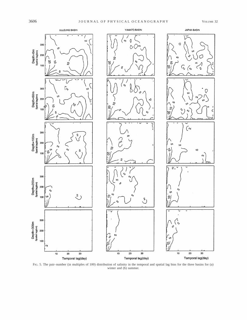
Taking the YB as an example, P(m, n) of surfacetemperature is greater than 2000 in most bins in winter(Fig. 4a) and summer (Fig. 5a). The maximum P(m, n)is located in bins near temporal lags 1–2 day and spatiallags 80–120 km for temperature (Figs. 4a and 5a), and1–2 day and 20–80 km for salinity (Figs. 4b and 5b);P(m, n) usually decreases with depth. Its values at depth300 m are about half of those at the surface. Further-more, in UB below 100 m, P(m, n) is too small (200in most bins) to perform the ACF computation.
5. ACFs of the JES thermohaline fields
a. Temperature
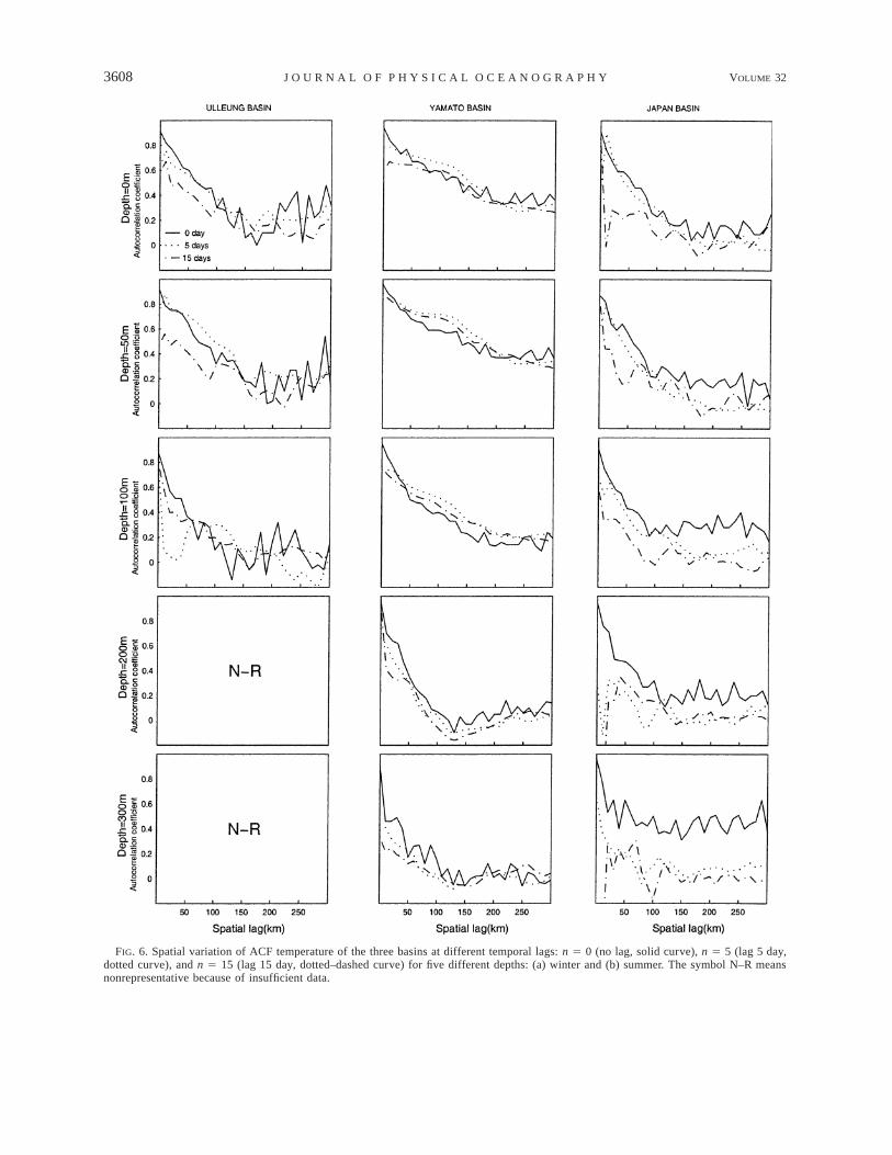
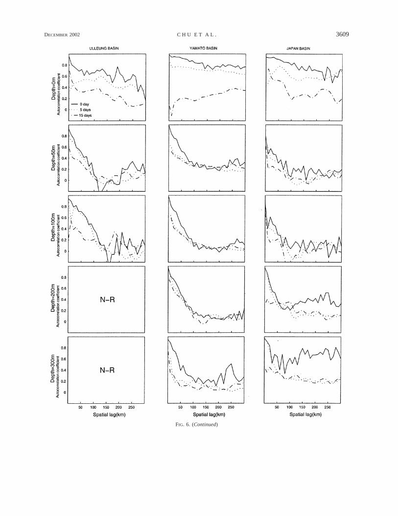
The spatial dependence of ACF temperature, h(z)(t, r),is obtained at several different temporal lags: t 5 0 (‘‘nolag’’), 5, and 15 days. The ACFs are plotted for differentseasons and five depths (z 5 0, 50, 100, 200, and 300m) in order to see the seasonal and vertical variations(Fig. 6). The depths are divided into three groups: surface(0 m), subsurface (50–200 m), and deep (300 m andbelow). A given depth is used only if the number ofobservations at that depth is greater than 3000.
The ACF temperature for the three basins has thefollowing features: 1) Its values are larger with no tem-poral lag (solid curves in Fig. 6) than with temporallags (dotted and dashed–dotted curves in Fig. 6); 2) Itdecreases with the spatial lag r for all seasons and forall depths except in UB, where it increases with r whenr . 150 km; 3) At the surface, the decrease of the ACFwith spatial lag r is moderate, indicating less spatialvariability; and 4) The ACF decreases faster with spatiallag r in the subsurface layers for all seasons.
1) JAPAN BASIN
The number of temperature observations is greaterthan 4000 from the surface to depth 300 m and muchless than 4000 below 300 m (Fig. 3a). Thus, it is rea-sonable to present the ACF temperature from the surfaceto 300 m. The ACF temperature (Fig. 6) has the fol-lowing features.
(i) Seasonal variability at the surface. At the surface,decrease of ACF temperature with the spatial lag r isslower in the summer than in the winter. For example,
DECEMBER 2002 3601C H U E T A L .
TABLE 2. Number of salinity profiles in the database for eachbasin and each season.
JB UB YB
WinterSpringSummerFall
2551545957183820
2706421240983836
3427513254483942
h (0)(0, r) decreases from 0.95 (r 5 0) to 0.78 (r 5 200km) in the summer (only 0.17 reduction), and from 0.9(r 5 0) to 0.10 (r 5 200 km) in the winter (0.8 reduc-tion). This indicates that SST has less spatial variabilityin the summer than in the winter.
(ii) Weak vertical variability from the surface to thesubsurface in the winter. The ACF temperature variesslightly from the surface to 200-m depth (Fig. 6a), in-dicating a relatively uniform thermal structure in ver-tical. However, in the summer, the ACF temperaturechanges drastically from the surface from the subsurface(50–200-m depth; Fig. 6b).
(iii) High spatial coherence in the deep layer. Forboth summer and winter, h (0)(0, r) at 300 m is greaterthan 0.4 for all r and is usually larger than that at theother depths except at the surface in the summer. Thisindicates that the spatial coherence is higher at 300 mthan at the other depths. The high spatial coherence inthe deep layer is consistent with the concept of JESProper Water proposed by Moriyasu (1972).
2) ULLEUNG BASIN
The number of temperature observations is greaterthan 3000 from the surface to 100-m depth, and muchless than 3000 below 100-m depth (Fig. 3a). Thus, it isreasonable to present the ACF temperature from thesurface to 100 m. The ACF temperature (Fig. 6) has thefollowing features.
(i) Seasonal variability at the surface. At the surface,there is less spatial variability in the summer than inthe winter. For example, h (0)(0, r) decreases from 0.95(r 5 0) to 0.47 (r 5 170 km) in the summer (0.48reduction), and decreases from 0.9 (r 5 0) to nearly 0(r 5 170 km) in the winter (0.9 reduction).
(ii) Less vertical variability from the surface to sub-surface in the winter. The ACF temperature variesslightly from the surface to 100-m depth (Fig. 6a), in-dicating a relatively uniform thermal structure in ver-tical. However, in the summer, the ACF temperaturechanges drastically from the surface to the subsurface(depth 50–100 m; Fig. 6b).
3) YAMATO BASIN
The number of temperature observations is greaterthan 4000 from the surface to 300-m depth, and muchless than 4000 below 300-m depth (Fig. 3a). Thus, it isreasonable to present the ACF-temperature from the sur-
face to 300 m. The ACF temperature (Fig. 6) has thefollowing features.
(i) Seasonal variability at the surface. As in the JBand UB, there is less spatial variability in the summerthan in the winter. For example, h (0)(0, r) is greater than0.7 for all r in the summer, and decreases from 0.95 (r5 0) to 0.3 (r 5 200 km) in the winter.
(ii) Reduction of spatial coherence with depth. Unlikein the JB, the ACF temperature generally decreases withdepth, and does not reveal high values at 300-m depth.This reflects the greatest depth of the JES Proper Waterin the YB than in the JB.
b. Salinity
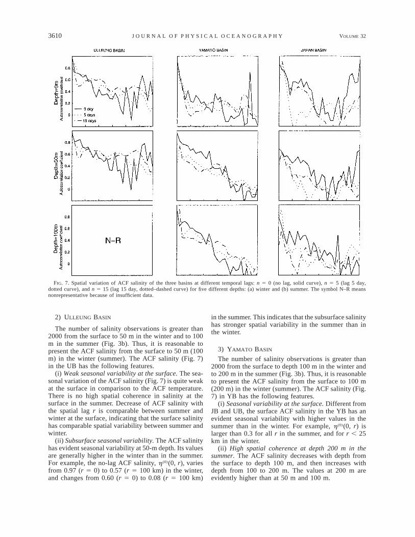
The estimate of ACF salinity is not as good as theestimate of ACF temperature because the number ofsalinity observations is less than the number of tem-perature observations (cf. Fig. 3b to Fig. 3a). The spatialdependence of ACF salinity, h (z)(t, r) is obtained for 0,5, and 15 day lags. The ACFs are plotted for differentseasons and five depths (z 5 0, 50, 100, 200, and 300m; Fig. 7). The depth is picked up only if the numberof observations at that depth larger than 2000. The ACFsalinity for the three basins is similar to the ACF tem-perature.
1) JAPAN BASIN
The number of salinity observations is greater than2000 from the surface to 100 m depth in the winter andto 300 m in the summer (Fig. 3b). Thus, it is reasonableto present the ACF salinity from the surface to 100 m(300 m) depth in the winter (summer).
(i) Weak seasonal variability. The seasonal variationof the ACF salinity (Fig. 7) is quite weak at all depthsin comparison to the ACF temperature. There is no highspatial coherence in salinity at the surface in the summer.Decrease of ACF salinity with the spatial lag r is com-parable between summer and winter at all depths. Forexample, h (0)(0, r) at the surface decreases from 0.90(r 5 0) to 0.18 (r 5 150 km) in the summer (0.72reduction), and decreases from 0.82 (r 5 0) to 0.04 (r5 150 km) in the winter (0.78 reduction). This indicatesthat SST has comparable spatial variability in summerand winter.
(ii) Weak vertical variability. The ACF salinity variesslightly with depth (Fig. 7), indicating a relatively uni-form haline structure in the vertical.
(iii) High spatial coherence at deep layer. Due to thedata sparseness, the ACF salinity estimate at 300-mdepth may be representative only in the summer (Fig.7b). Its values at 300-m depth are greater than 0.4 forr , 220 km, indicating high spatial coherence. Thisfeature is similar to the ACF temperature in JB.
3602 VOLUME 32J O U R N A L O F P H Y S I C A L O C E A N O G R A P H Y
FIG. 3. Depth dependence of number of observations for (a) temperature and (b) salinity.
DECEMBER 2002 3603C H U E T A L .
FIG. 3. (Continued)
3604 VOLUME 32J O U R N A L O F P H Y S I C A L O C E A N O G R A P H Y
FIG. 4. The pair–number (in multiples of 100) distribution of temperature in the temporal and spatial lag bins for the three basins for (a)winter and (b) summer.
DECEMBER 2002 3605C H U E T A L .
FIG. 4. (Continued)
3606 VOLUME 32J O U R N A L O F P H Y S I C A L O C E A N O G R A P H Y
FIG. 5. The pair–number (in multiples of 100) distribution of salinity in the temporal and spatial lag bins for the three basins for (a)winter and (b) summer.
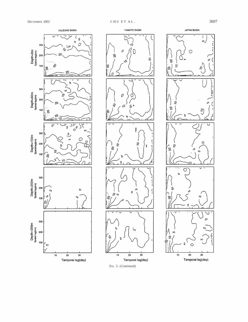
DECEMBER 2002 3607C H U E T A L .
FIG. 5. (Continued)
3608 VOLUME 32J O U R N A L O F P H Y S I C A L O C E A N O G R A P H Y
FIG. 6. Spatial variation of ACF temperature of the three basins at different temporal lags: n 5 0 (no lag, solid curve), n 5 5 (lag 5 day,dotted curve), and n 5 15 (lag 15 day, dotted–dashed curve) for five different depths: (a) winter and (b) summer. The symbol N–R meansnonrepresentative because of insufficient data.
DECEMBER 2002 3609C H U E T A L .
FIG. 6. (Continued)
3610 VOLUME 32J O U R N A L O F P H Y S I C A L O C E A N O G R A P H Y
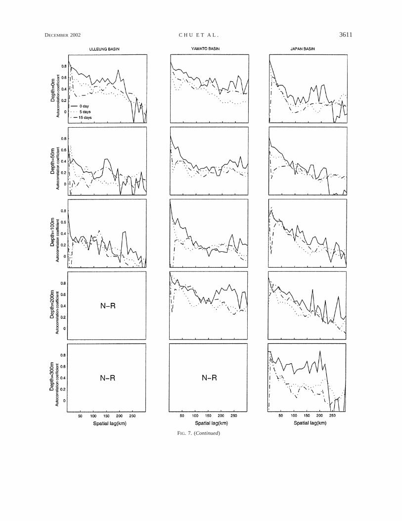
FIG. 7. Spatial variation of ACF salinity of the three basins at different temporal lags: n 5 0 (no lag, solid curve), n 5 5 (lag 5 day,dotted curve), and n 5 15 (lag 15 day, dotted–dashed curve) for five different depths: (a) winter and (b) summer. The symbol N–R meansnonrepresentative because of insufficient data.
2) ULLEUNG BASIN
The number of salinity observations is greater than2000 from the surface to 50 m in the winter and to 100m in the summer (Fig. 3b). Thus, it is reasonable topresent the ACF salinity from the surface to 50 m (100m) in the winter (summer). The ACF salinity (Fig. 7)in the UB has the following features.
(i) Weak seasonal variability at the surface. The sea-sonal variation of the ACF salinity (Fig. 7) is quite weakat the surface in comparison to the ACF temperature.There is no high spatial coherence in salinity at thesurface in the summer. Decrease of ACF salinity withthe spatial lag r is comparable between summer andwinter at the surface, indicating that the surface salinityhas comparable spatial variability between summer andwinter.
(ii) Subsurface seasonal variability. The ACF salinityhas evident seasonal variability at 50-m depth. Its valuesare generally higher in the winter than in the summer.For example, the no-lag ACF salinity, h (0)(0, r), variesfrom 0.97 (r 5 0) to 0.57 (r 5 100 km) in the winter,and changes from 0.60 (r 5 0) to 0.08 (r 5 100 km)
in the summer. This indicates that the subsurface salinityhas stronger spatial variability in the summer than inthe winter.
3) YAMATO BASIN
The number of salinity observations is greater than2000 from the surface to depth 100 m in the winter andto 200 m in the summer (Fig. 3b). Thus, it is reasonableto present the ACF salinity from the surface to 100 m(200 m) in the winter (summer). The ACF salinity (Fig.7) in YB has the following features.
(i) Seasonal variability at the surface. Different fromJB and UB, the surface ACF salinity in the YB has anevident seasonal variability with higher values in thesummer than in the winter. For example, h (0)(0, r) islarger than 0.3 for all r in the summer, and for r , 25km in the winter.
(ii) High spatial coherence at depth 200 m in thesummer. The ACF salinity decreases with depth fromthe surface to depth 100 m, and then increases withdepth from 100 to 200 m. The values at 200 m areevidently higher than at 50 m and 100 m.
DECEMBER 2002 3611C H U E T A L .
FIG. 7. (Continued)
3612 VOLUME 32J O U R N A L O F P H Y S I C A L O C E A N O G R A P H Y
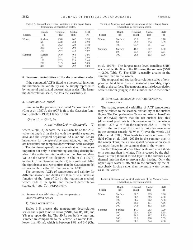
TABLE 3. Seasonal and vertical variations of the Japan Basintemperature decorrelation scales.
SeasonDepth
(m)Temporal
(day)Spatial(km)
SNR(l)
Winter Surface50100200300
23.024.026.224.226.4
242228220204222
3.182.593.183.964.90
Summer Surface50100200300
16.024.127.531.536.2
464238223248292
3.962.002.485.695.69
TABLE 4. Seasonal and vertical variations of the Ulleung Basintemperature decorrelation scales.
SeasonDepth
(m)Temporal
(day)Spatial(km)
SNR(l)
Winter Surface50100
23.825.127.4
251254211
3.183.392.71
Summer Surface50100
18.131.428.6
307247213
4.903.643.96
TABLE 5. Seasonal and vertical variations of the Yamato Basintemperature decorrelation scales.
SeasonDepth
(m)Temporal
(day)Spatial(km)
SNR(l)
Winter Surface50100200300
30.536.936.230.024.5
309315262191192
3.964.904.364.363.18
Summer Surface50100200300
14.725.429.031.030.3
963276187200324
7.009.959.955.694.36
6. Seasonal variabilities of the decorrelation scales
If the computed ACF is fitted to a theoretical function,the thermohaline variability can be simply representedby temporal and spatial decorrelation scales. The largerthe decorrelation scale, the less the variability is.
a. Gaussian ACF model
Similar to the previous calculated Yellow Sea ACF(Chu et al. 1997b), the ACF is fit to the Gaussian func-tion (Phoebus 1988; Clancy 1983):
(z) (z)h (m, n) 5 h (0, 0)2 2 2 23 exp[2A (mDr) 2 C (nDt) ], (2)z z
where (z)(m, n) denotes the Gaussian fit of the ACFhvalue (at depth z) in the bin with the spatial separationmDr and the temporal separation nDt. Dr and Dt areincrements for the space/time separation; and21 21A Cz z
are horizontal and temporal decorrelation scales at depthz. The dominant space/time scales obtained from h areimportant not only in determining sampling density butalso in the optimum interpolation of the observed data.We use the same F test depicted in Chu et al. (1997b)to check if the Gaussian model (2) is significant. Afterthe significance test, we confirm that the Gaussian modelis reasonable for the JES thermohaline ACF.
The computed ACFs of temperature and salinity fordifferent seasons and depths are then fit to a Gaussianfunction of the form of (2) by the regression method,which leads to the spatial and temporal decorrelationscales, and , respectively.21 21A Cz z
b. Seasonal variabilities of the temperaturedecorrelation scales
1) CHARACTERISTICS
Tables 3–5 present the temperature decorrelationscales and signal to noise ratios (SNRs) for JB, UB, andYB (see appendix B). The SNRs for both winter andsummer are comparable to the Yellow Sea waters (shal-lower than 80 m), which is between 1.88 and 3.0 (Chu
et al. 1997b). The largest noise level (smallest SNR)occurs at depth 50 m in the JB during the summer (SNR5 2.00, Table 3). The SNR is usually greater in thesummer than in the winter.
The temporal and spatial decorrelation scales of tem-perature field have evident seasonal variability, espe-cially at the surface. The temporal (spatial) decorrelationscale is shorter (longer) in the summer than in the winter.
2) PHYSICAL MECHANISM FOR THE SEASONAL
VARIABILITY
The strong seasonal variability of ACF temperaturemay be related to the seasonal variability of the surfacefluxes. The Comprehensive Ocean and Atmosphere DataSet (COADS) shows that the net surface heat flux(downward positive) is inhomogeneous in the winter(from 2275 W m22 in the southeast JES to 2150 Wm22 in the northwest JES), and is quite homogeneousin the summer (nearly 75 W m22) over the whole JES(Slutz et al. 1985). This leads to a more uniform SSTfield (Chu et al. 1998, 2001b) in the summer than inthe winter. Thus, the surface spatial decorrelation scalesare much larger in the summer than in the winter.
Surface temporal decorrelation scales are much short-er in summer than in winter. This is caused by the shal-lower surface thermal mixed layer in the summer (lessthermal inertia) due to strong solar heating. Only theupper-layer water is affected in the summer by the at-mospheric forcing rather than the entire water columnas in the winter.
DECEMBER 2002 3613C H U E T A L .
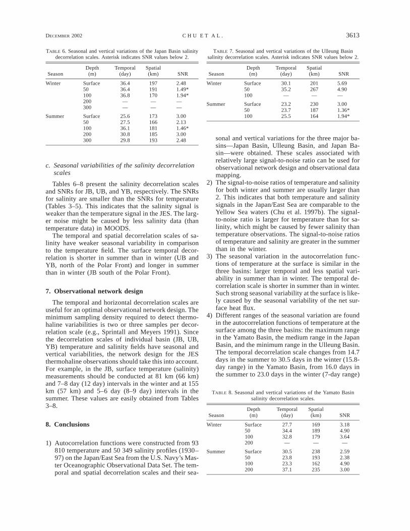
TABLE 6. Seasonal and vertical variations of the Japan Basin salinitydecorrelation scales. Asterisk indicates SNR values below 2.
SeasonDepth
(m)Temporal
(day)Spatial(km) SNR
Winter Surface50100200300
36.436.436.8——
197191170——
2.481.49*1.94*——
Summer Surface50100200300
25.627.536.130.829.8
173166181185193
3.002.131.46*3.002.48
TABLE 7. Seasonal and vertical variations of the Ulleung Basinsalinity decorrelation scales. Asterisk indicates SNR values below 2.
SeasonDepth
(m)Temporal
(day)Spatial(km) SNR
Winter Surface50100
30.135.2—
201267—
5.694.90—
Summer Surface50100
23.223.725.5
230187164
3.001.36*1.94*
TABLE 8. Seasonal and vertical variations of the Yamato Basinsalinity decorrelation scales.
SeasonDepth
(m)Temporal
(day)Spatial(km) SNR
Winter Surface50100200
27.734.432.8—
169189179—
3.184.903.64—
Summer Surface50100200
30.523.823.337.1
238193162235
2.592.384.903.00
c. Seasonal variabilities of the salinity decorrelationscales
Tables 6–8 present the salinity decorrelation scalesand SNRs for JB, UB, and YB, respectively. The SNRsfor salinity are smaller than the SNRs for temperature(Tables 3–5). This indicates that the salinity signal isweaker than the temperature signal in the JES. The larg-er noise might be caused by less salinity data (thantemperature data) in MOODS.
The temporal and spatial decorrelation scales of sa-linity have weaker seasonal variability in comparisonto the temperature field. The surface temporal decor-relation is shorter in summer than in winter (UB andYB, north of the Polar Front) and longer in summerthan in winter (JB south of the Polar Front).
7. Observational network design
The temporal and horizontal decorrelation scales areuseful for an optimal observational network design. Theminimum sampling density required to detect thermo-haline variabilities is two or three samples per decor-relation scale (e.g., Sprintall and Meyers 1991). Sincethe decorrelation scales of individual basin (JB, UB,YB) temperature and salinity fields have seasonal andvertical variabilities, the network design for the JESthermohaline observations should take this into account.For example, in the JB, surface temperature (salinity)measurements should be conducted at 81 km (66 km)and 7–8 day (12 day) intervals in the winter and at 155km (57 km) and 5–6 day (8–9 day) intervals in thesummer. These values are easily obtained from Tables3–8.
8. Conclusions
1) Autocorrelation functions were constructed from 93810 temperature and 50 349 salinity profiles (1930–97) on the Japan/East Sea from the U.S. Navy’s Mas-ter Oceanographic Observational Data Set. The tem-poral and spatial decorrelation scales and their sea-
sonal and vertical variations for the three major ba-sins—Japan Basin, Ulleung Basin, and Japan Ba-sin—were obtained. These scales associated withrelatively large signal-to-noise ratio can be used forobservational network design and observational datamapping.
2) The signal-to-noise ratios of temperature and salinityfor both winter and summer are usually larger than2. This indicates that both temperature and salinitysignals in the Japan/East Sea are comparable to theYellow Sea waters (Chu et al. 1997b). The signal-to-noise ratio is larger for temperature than for sa-linity, which might be caused by fewer salinity thantemperature observations. The signal-to-noise ratiosof temperature and salinity are greater in the summerthan in the winter.
3) The seasonal variation in the autocorrelation func-tions of temperature at the surface is similar in thethree basins: larger temporal and less spatial vari-ability in summer than in winter. The temporal de-correlation scale is shorter in summer than in winter.Such strong seasonal variability at the surface is like-ly caused by the seasonal variability of the net sur-face heat flux.
4) Different ranges of the seasonal variation are foundin the autocorrelation functions of temperature at thesurface among the three basins: the maximum rangein the Yamato Basin, the medium range in the JapanBasin, and the minimum range in the Ulleung Basin.The temporal decorrelation scale changes from 14.7days in the summer to 30.5 days in the winter (15.8-day range) in the Yamato Basin, from 16.0 days inthe summer to 23.0 days in the winter (7-day range)
3614 VOLUME 32J O U R N A L O F P H Y S I C A L O C E A N O G R A P H Y
in the Japan Basin, and from 18.1 days in the summerto 23.8 days in the winter (5.7-day range) in theUlleung Basin. The spatial decorrelation scalechanges from 963 km in the summer to 309 km inthe winter (654-km range) in the Yamato Basin, from464 km in the summer to 242 km in the winter (222km range) in the Japan Basin, and from 307 km inthe summer to 251 km in the winter (56-km range)in the Ulleung Basin.
5) Among the three basins, the spatial thermal vari-ability is weakest in the Yamato Basin (spatial de-correlation scale ranging from 309 to 963 km) forall seasons, strongest in the Ulleung Basin in thesummer (spatial decorrelation scale around 307 km),and strongest in the Japan Basin in the winter (spatialdecorrelation scale around 242 km). In the winter,the temporal thermal variability is weaker in the Ya-mato Basin (temporal decorrelation scale around30.5 days) than in the Japan and Ulleung Basins(temporal decorrelation scale around 23–24 days).In the summer, the temporal thermal variability isweaker in the Ulleung Basin (temporal decorrelationscale around 18.1 days) than in the Japan Basin (16days) and Yamato Basins (14.7 days).
6) The autocorrelation functions of salinity for the threebasins have weaker seasonal variability in compar-ison to that of the temperature field. The surfacetemporal decorrelation has different seasonal varia-tions among the three basins: shorter in summer(23.2 days in Ulleung Basin and 16.0 days in JapanBasin) and longer in winter (30.1 days in UlleungBasin and 23.0 days in Japan Basin), except in theYamato Basin, where it is longer in the summer (30.5days) and shorter in the winter (27.7 days). The sur-face spatial decorrelation scales are 173 (197), 230(201), and 238 (169) km in the Japan, Ulleung, andYamato Basins during the summer (winter).
7) In the Japan Basin, high spatial coherence is foundin the deep layer (300 m) for temperature and salin-ity, consistent with the concept of JES Proper Waterproposed by Moriyasu (1972). In the Yamato Basin,high spatial coherence of salinity is found at depth200 m in the summer.
8) The temporal and horizontal decorrelation scales areuseful for designing an optimal observational net-work. Since the decorrelation scales of the temper-ature and salinity fields have an evident layered char-acteristics (larger values in the upper layer and small-er values in the intermediate layer), we should usedifferent sampling densities. The minimum samplingdensity to detect temperature and salinity variabili-ties (one-third of the decorrelation scales) for eachbasin can be obtained from Tables 3–8.
Acknowledgments. The authors are grateful to LynneTalley (the editor) for suggestions and two anonymousreviewers for comments on the preliminary draft. This
work was funded by the Naval Oceanographic Office,the Office of Naval Research, and the Naval Postgrad-uate School, Wang Guihua also wishes to acknowledgethe support by the key project, No. G1999043805, fromChina.
APPENDIX A
ACF Estimation
The ACF value for each bin (t, r) is estimated by(z) (z)c 9c 9O o o
bin (t,r)(z)h (t, r) 5 , (A1)(z) 2[c 9]O o
bin(t,r)
which varies with the spatial and temporal lags (t, r)and depth z. Whether the computed h (z)(t, r) is statis-tically significant should be tested by
ta(z)h (t, r) [ (A2)a(z) 2ÏP (t, r) 2 2 1 ta
with the significance level of a and the t distribution of[P (z)(t, r) 2 2] degrees of freedom (Chu et al. 1997b).When h (z)(t, r) . ha, the estimated ACF is significanton the level of a. Since both h (z)(t, r) and (t, r) have(z)ha
seasonal variations, the significance of the ACF esti-mation should also change with seasons. SignificantACF estimation (a 5 0.10) is limited to the areas onthe (t, r) plane with positive values of
(z) (z)Dh 5 h (t, r) 2 h (t, r)a (A3)
and is not significant for areas with negative values.
APPENDIX B
Signal-to-Noise Ratio (SNR)
The measured variance s2 of the thermal fields is sep-arated into signal and noise, whereby
2 2 2s 5 s 1 s .s n
The noise variance has two sources, geophysical andinstrumentation errors. Here, the geophysical error isunresolved thermal variability with scales smaller thanthe typical time and space scales between two temper-ature profiles. In this study the unresolved scales are 0.5day and 5 km. The ACF value in the first bin (0, 0)does not represent the correlation between profilespaired by themselves, and therefore does not equal 1.Following Sprintall and Meyers (1991) the signal-to-noise ratio is computed by
s h(0, 0)sl [ 5 . (B1)!s 1 2 h(0, 0)n
The larger the l, the smaller the geophysical error. Ifh(0, 0) 5 1, there is no noise and l 5 `. If h(0, 0) 50, there is no signal. If l . 2, the ratio of the signal
DECEMBER 2002 3615C H U E T A L .
variance, , to the noise variance, , is greater than 4,2 2s ss n
which was considered quite good by White et al. (1982)and Sprintall and Meyers (1991).
REFERENCES
Chu, P. C., 1995: P-vector method for determining absolute velocityfrom hydrographic data. Mar. Technol. Soc. J., 29 (3), 3–14.
——, H.-C. Tseng, C. P. Chang, and J. M. Chen, 1997a: South ChinaSea warm pool detected in spring from the Navy’s Master Ocean-ographic Observational Data Set (MOODS). J. Geophys. Res.,102, 15 761–15 771.
——, S. K. Wells, S. D. Haeger, C. Szczechowski, and M. Carron,1997b: Temporal and spatial scales of the Yellow Sea thermalvariability. J. Geophys. Res., 102, 5655–5668.
——, Y. C. Chen, and S. H. Lu, 1998: Temporal and spatial vari-abilities of Japan Sea surface temperature and atmospheric forc-ing. J. Oceanogr., 54, 273–284.
——, J. Lan, and C. W. Fan, 2001a: Japan/East Sea circulation andthermohaline structure. Part II: A variational P-vector method.J. Phys. Oceanogr., 31, 2886–2902.
——, ——, and ——, 2001b: Japan Sea circulation and thermohalinestructure. Part I: Climatology. J. Phys. Oceanogr., 31, 244–271.
Clancy, R. M., 1983: The effect of observational error correlationson objective analysis of ocean thermal structure. Deep-Sea Res.,30, 985–1002.
Hase, H., J.-H. Yoon, and W. Koterayama, 1999: The current structureof the Tsushima Warm Current along the Japanese coast. J.Oceanogr., 55, 217–235.
Hong, C. H., K. D. Cho, and S. K. Yang, 1984: On the abnormalcooling phenomenon in the coastal areas of East Sea of Koreain the summer 1981. J. Oceanol. Soc. Korea, 19, 11–17.
Isoda, Y., and S. Saitoh, 1988: Variability of the sea surface tem-perature obtained by the statistical analysis of AVHRR imag-ery—A case study of the south Japan Sea. J. Oceanogr. Soc.Japan, 44, 52–59.
——, and ——, 1993: The northward intruding eddy along the eastcoast of Korea. J. Oceanogr., 49, 443–458.
Kano, Y., 1980: The annual variation of the temperature, salinity andoxygen contents in the Japan Sea. Oceanogr. Mag., 31, 15–26.
Kawabe, M., 1982a: Branching of the Tsushima Current in the JapanSea, Part I: Data analysis. J. Oceanogr. Soc. Japan, 38, 95–107.
——, 1982b: Branching of the Tsushima Current in the Japan Sea,Part II: Numerical experiment. J. Oceanogr. Soc. Japan, 38,183–192.
Kim, K., and J. Y. Chung, 1984: On the salinity-minimum and dis-solved oxygen-maximum layer in the East Sea (Sea of Japan).Ocean Hydrodynamics of the Japan and East China Seas, T.Ichiye, Ed., Elsevier Science, 55–65.
——, Y.-G. Kim, Y.-K. Cho, M. Takematsu, and Y. Volkov, 1999:Basin-to-basin and year-to-year variation of temperature and sa-linity characteristics in the East Sea (Sea of Japan). J. Oceanogr.,55, 103–109.
Kim, Y.-G., and K. Kim, 1999: Intermediate Waters in the East/JapanSea. J. Oceanogr., 55, 123–132.
Maizuru Marine Observatory, 1997: Climate chart of the Japan Sea.Maizuru, Japan.
Martin, S., and M. Kawase, 1998: The southern flux of sea ice in theTatarskiy Strait, Japan Sea and the generation of the Liman Cur-rent. J. Mar. Res., 56, 141–155.
Miyazaki, M., 1953: On the water masses of the Japan Sea (in Jap-anese with English abstract). Bull. Hokkaido Reg. Fish. Res.Lab., 7, 1–65.
Moriyasu, S., 1972: The Tsushima current. Kuroshio, Its PhysicalAspects, H. M. Stommel and K. Yoshida, Eds., University ofTokyo Press, 353–369.
Phoebus, P. A., 1988: Improvements to the data selection algorithmsin the Optimum Thermal Interpolation System (OTIS). NavalOcean Research and Development Activity Rep. 239, 18 pp.
Senjyu, T., 1999: The Japan Sea Intermediate Water: Its characteristicsand circulation. J. Oceanogr., 55, 111–122.
Seung, Y.-H., 1994: The separation of the East Korean Warm Currentand the mechanism for the formation of the North Korean ColdCurrent (in Japanese). Kaiyo Mon., 9, 758–765.
Slutz, R. J., S. J. Lubker, J. D. Hiscox, S. D. Woodruff, R. L. Jenne,D. H. Joseph, P. M. Steurer, and J. D. Elms, 1985: ComprehensiveOcean–Atmosphere Data Set. CIRES/ERL/NCAR/NCDC, 268pp.
Sprintall, J., and G. Meyers, 1991: An optimal XBT sampling networkfor the eastern Pacific Ocean. J. Geophys. Res., 96, 10 539–10 552.
Teague, W. J., M. J. Carron, and P. J. Hogan, 1990: A comparisonbetween the Generalized Digital Environmental Model and Lev-itus climatologies. J. Geophys. Res., 95, 7167–7183.
Uda, M., 1934: The results of simultaneous oceanographic investi-gations in the Japan Sea and its adjacent waters in May and June,1932 (in Japanese). J. Imp. Fish. Exp. Stn., 5, 57–190.
White, W. B., G. Meyers, and K. Hasunuma, 1982: Space/time sta-tistics of short-term climatic variability in the western NorthPacific. J. Geophys. Res., 87, 1979–1989.
Yoon, J.-H., 1982: Numerical experiment on the circulation in theJapan Sea, Part I. Formation of the East Korean Warm Current.J. Oceanogr. Soc. Japan, 38, 43–51.