Embed Size (px)
Citation preview
DECENTRALIZED CONTROL OF NETWORKS OF UNCERTAIN DYNAMICALSYSTEMS
By
JUSTIN RICHARD KLOTZ
A DISSERTATION PRESENTED TO THE GRADUATE SCHOOLOF THE UNIVERSITY OF FLORIDA IN PARTIAL FULFILLMENT
OF THE REQUIREMENTS FOR THE DEGREE OFDOCTOR OF PHILOSOPHY
UNIVERSITY OF FLORIDA
2015

c© 2015 Justin Richard Klotz
2

To my parents, Rick and Karen, my sister, Heather, and my friends, for their boundlesssupport and encouragement
3

ACKNOWLEDGMENTS
I would like to express my sincere gratitude to Dr. Warren E. Dixon, whose advice
and motivation were essential to my academic success. As my advisor, he has guided
my research and encouraged the creativity that helped shape this dissertation. As a
mentor, he has helped me choose the direction of my career and develop professionally.
I would also like to extend gratitude to my committee members Dr. Prabir Barooah, Dr.
Carl Crane, and Dr. John Shea for their valuable recommendations and insights. I am
also thankful to my family and friends for their enduring support and to my coworkers in
the Nonlinear Controls and Robotics laboratory for our fruitful collaboration.
4
TABLE OF CONTENTS
page
ACKNOWLEDGMENTS . . . . . . . . . . . . . . . . . . . . . . . . . . . . . . . . . . 4
LIST OF TABLES . . . . . . . . . . . . . . . . . . . . . . . . . . . . . . . . . . . . . . 8
LIST OF FIGURES . . . . . . . . . . . . . . . . . . . . . . . . . . . . . . . . . . . . . 9
LIST OF ABBREVIATIONS . . . . . . . . . . . . . . . . . . . . . . . . . . . . . . . . 11
ABSTRACT . . . . . . . . . . . . . . . . . . . . . . . . . . . . . . . . . . . . . . . . . 12
CHAPTER
1 INTRODUCTION . . . . . . . . . . . . . . . . . . . . . . . . . . . . . . . . . . . 14
1.1 Motivation . . . . . . . . . . . . . . . . . . . . . . . . . . . . . . . . . . . . 141.2 Literature Review . . . . . . . . . . . . . . . . . . . . . . . . . . . . . . . . 181.3 Contributions . . . . . . . . . . . . . . . . . . . . . . . . . . . . . . . . . . 221.4 Preliminaries . . . . . . . . . . . . . . . . . . . . . . . . . . . . . . . . . . 25
2 ASYMPTOTIC SYNCHRONIZATION OF A LEADER-FOLLOWER NETWORKSUBJECT TO UNCERTAIN DISTURBANCES . . . . . . . . . . . . . . . . . . . 26
2.1 Problem Formulation . . . . . . . . . . . . . . . . . . . . . . . . . . . . . . 262.1.1 Dynamic Models and Properties . . . . . . . . . . . . . . . . . . . . 262.1.2 Control Objective . . . . . . . . . . . . . . . . . . . . . . . . . . . . 28
2.2 Controller Development . . . . . . . . . . . . . . . . . . . . . . . . . . . . 302.3 Convergence Analysis . . . . . . . . . . . . . . . . . . . . . . . . . . . . . 332.4 Simulation . . . . . . . . . . . . . . . . . . . . . . . . . . . . . . . . . . . . 382.5 Extension to Formation Control . . . . . . . . . . . . . . . . . . . . . . . . 43
2.5.1 Modified Error Signal . . . . . . . . . . . . . . . . . . . . . . . . . . 432.5.2 Simulation . . . . . . . . . . . . . . . . . . . . . . . . . . . . . . . . 44
2.6 Concluding Remarks . . . . . . . . . . . . . . . . . . . . . . . . . . . . . . 49
3 ROBUST CONTAINMENT CONTROL IN A LEADER-FOLLOWER NETWORKOF UNCERTAIN EULER-LAGRANGE SYSTEMS . . . . . . . . . . . . . . . . 50
3.1 Problem Formulation . . . . . . . . . . . . . . . . . . . . . . . . . . . . . . 503.1.1 Notation for a Multi-Leader Network . . . . . . . . . . . . . . . . . . 503.1.2 Dynamic Models and Properties . . . . . . . . . . . . . . . . . . . . 513.1.3 Control Objective . . . . . . . . . . . . . . . . . . . . . . . . . . . . 53
3.2 Controller Development . . . . . . . . . . . . . . . . . . . . . . . . . . . . 543.3 Convergence Analysis . . . . . . . . . . . . . . . . . . . . . . . . . . . . . 583.4 Simulation . . . . . . . . . . . . . . . . . . . . . . . . . . . . . . . . . . . . 633.5 Concluding Remarks . . . . . . . . . . . . . . . . . . . . . . . . . . . . . . 67
5
4 SYNCHRONIZATION OF UNCERTAIN EULER-LAGRANGE SYSTEMS WITHUNCERTAIN TIME-VARYING COMMUNICATION DELAYS . . . . . . . . . . . 68
4.1 Problem Formulation . . . . . . . . . . . . . . . . . . . . . . . . . . . . . . 694.1.1 Dynamic Models and Properties . . . . . . . . . . . . . . . . . . . . 694.1.2 Control Objective . . . . . . . . . . . . . . . . . . . . . . . . . . . . 71
4.2 Controller Development . . . . . . . . . . . . . . . . . . . . . . . . . . . . 714.2.1 Communication-Delayed Control . . . . . . . . . . . . . . . . . . . 714.2.2 Motivating Example . . . . . . . . . . . . . . . . . . . . . . . . . . . 73
4.3 Closed-loop Error System . . . . . . . . . . . . . . . . . . . . . . . . . . . 754.4 Convergence Analysis . . . . . . . . . . . . . . . . . . . . . . . . . . . . . 784.5 Simulation . . . . . . . . . . . . . . . . . . . . . . . . . . . . . . . . . . . . 914.6 Concluding Remarks . . . . . . . . . . . . . . . . . . . . . . . . . . . . . . 96
5 DECENTRALIZED SYNCHRONIZATION OF UNCERTAIN NONLINEAR SYS-TEMS WITH A REPUTATION ALGORITHM . . . . . . . . . . . . . . . . . . . . 98
5.1 Problem Formulation . . . . . . . . . . . . . . . . . . . . . . . . . . . . . . 985.1.1 Network Properties . . . . . . . . . . . . . . . . . . . . . . . . . . . 985.1.2 Dynamic Models and Properties . . . . . . . . . . . . . . . . . . . . 995.1.3 Neighbor Communication and Sensing . . . . . . . . . . . . . . . . 1005.1.4 Control Objective . . . . . . . . . . . . . . . . . . . . . . . . . . . . 101
5.2 Controller Development . . . . . . . . . . . . . . . . . . . . . . . . . . . . 1015.2.1 Error System . . . . . . . . . . . . . . . . . . . . . . . . . . . . . . 1015.2.2 Decentralized Controller . . . . . . . . . . . . . . . . . . . . . . . . 1025.2.3 Reputation Algorithm . . . . . . . . . . . . . . . . . . . . . . . . . . 1025.2.4 Edge Weight Updates . . . . . . . . . . . . . . . . . . . . . . . . . 104
5.3 Closed-loop Error System . . . . . . . . . . . . . . . . . . . . . . . . . . . 1055.4 Convergence Analysis . . . . . . . . . . . . . . . . . . . . . . . . . . . . . 1075.5 Satisfaction of Sufficient Conditions . . . . . . . . . . . . . . . . . . . . . . 112
5.5.1 A Lower Bound on the Solution of the CALE . . . . . . . . . . . . . 1125.5.2 An Upper Bound on the Solution of the CALE . . . . . . . . . . . . 1135.5.3 Computation of Sufficient Conditions . . . . . . . . . . . . . . . . . 115
5.6 Simulation . . . . . . . . . . . . . . . . . . . . . . . . . . . . . . . . . . . . 1165.7 Concluding Remarks . . . . . . . . . . . . . . . . . . . . . . . . . . . . . . 122
6 CONCLUSIONS AND FUTURE WORK . . . . . . . . . . . . . . . . . . . . . . 124
6.1 Conclusions . . . . . . . . . . . . . . . . . . . . . . . . . . . . . . . . . . . 1246.2 Future Work . . . . . . . . . . . . . . . . . . . . . . . . . . . . . . . . . . . 127
APPENDIX
A Proof that P is Nonnegative (CH 2) . . . . . . . . . . . . . . . . . . . . . . . . . 129
B Proof of Supporting Lemma (CH 3) . . . . . . . . . . . . . . . . . . . . . . . . . 131
C Demonstration of Supporting Inequality (CH 4) . . . . . . . . . . . . . . . . . . 132
6
D Demonstration of Reputation Bound (CH 5) . . . . . . . . . . . . . . . . . . . . 134
E Proof of Supporting Lemma (CH 5) . . . . . . . . . . . . . . . . . . . . . . . . . 135
F Proof of Supporting Lemma (CH 5) . . . . . . . . . . . . . . . . . . . . . . . . . 137
REFERENCES . . . . . . . . . . . . . . . . . . . . . . . . . . . . . . . . . . . . . . . 138
BIOGRAPHICAL SKETCH . . . . . . . . . . . . . . . . . . . . . . . . . . . . . . . . 145
7

LIST OF TABLES
Table page
2-1 Simulation parameters. . . . . . . . . . . . . . . . . . . . . . . . . . . . . . . . 41
2-2 Controller performance comparison. . . . . . . . . . . . . . . . . . . . . . . . . 43
2-3 Disturbance and formation position parameters. . . . . . . . . . . . . . . . . . . 48
3-1 Leader initial positions in surge (x), sway (y), and heave (z). . . . . . . . . . . . 64
3-2 Follower initial positions in surge (x), sway (y), and heave (z). . . . . . . . . . . 65
4-1 Disturbance parameters. . . . . . . . . . . . . . . . . . . . . . . . . . . . . . . . 92
4-2 Communication delay and delay estimate parameters for each communica-tion link. . . . . . . . . . . . . . . . . . . . . . . . . . . . . . . . . . . . . . . . . 93
4-3 Tuned gains and associated costs for (a) feedback without self-delay, (b) onlyfeedback with self-delay, and (c) a mixture of feedback with self-delay andwithout self-delay. . . . . . . . . . . . . . . . . . . . . . . . . . . . . . . . . . . 94
5-1 Parameters in dynamics. . . . . . . . . . . . . . . . . . . . . . . . . . . . . . . . 119
5-2 Steady-state RMS leader-tracking performance. . . . . . . . . . . . . . . . . . 119
8
LIST OF FIGURES
Figure page
2-1 Network communication topology. . . . . . . . . . . . . . . . . . . . . . . . . . 40
2-2 Joint 1 leader-tracking error using (a) [1], (b) [2, Section IV], and (c) the pro-posed controller. . . . . . . . . . . . . . . . . . . . . . . . . . . . . . . . . . . . 41
2-3 Joint 2 leader-tracking error using (a) [1], (b) [2, Section IV], and (c) the pro-posed controller. . . . . . . . . . . . . . . . . . . . . . . . . . . . . . . . . . . . 42
2-4 Joint 1 control effort using (a) [1], (b) [2, Section IV], and (c) the proposed con-troller. . . . . . . . . . . . . . . . . . . . . . . . . . . . . . . . . . . . . . . . . . 42
2-5 Joint 2 control effort using (a) [1], (b) [2, Section IV], and (c) the proposed con-troller. . . . . . . . . . . . . . . . . . . . . . . . . . . . . . . . . . . . . . . . . . 43
2-6 Network communication topology. . . . . . . . . . . . . . . . . . . . . . . . . . 47
2-7 Agent trajectories in surge and sway. . . . . . . . . . . . . . . . . . . . . . . . . 48
2-8 Error in convergence to the formation positions in the dimensions surge, swayand yaw. . . . . . . . . . . . . . . . . . . . . . . . . . . . . . . . . . . . . . . . . 49
3-1 Network communication topology of leader (“L”) and follower (“F”) AUVs. . . . . 64
3-2 [Top view] Follower AUV trajectories in the surge (x) and sway (y) dimensions. 65
3-3 [Front view] Follower AUV trajectories in the surge (x) and heave (z) dimen-sions. . . . . . . . . . . . . . . . . . . . . . . . . . . . . . . . . . . . . . . . . . 66
3-4 Euclidean norms of the follower AUV control efforts. . . . . . . . . . . . . . . . 66
4-1 Network communication topology. . . . . . . . . . . . . . . . . . . . . . . . . . 74
4-2 Leader-tracking error under communication-delayed control using (a) onlyfeedback without self-delay, (b) only feedback with exact self-delay, and (c)only feedback with inexact self-delay. . . . . . . . . . . . . . . . . . . . . . . . . 75
4-3 Network communication topology. . . . . . . . . . . . . . . . . . . . . . . . . . 92
4-4 Leader-tracking error under communication-delayed closed-loop control usingonly feedback without self-delay (κ1 = 1, κ2 = 0). . . . . . . . . . . . . . . . . . 95
4-5 Leader-tracking error under communication-delayed closed-loop control usingonly feedback with self-delay (κ1 = 0, κ2 = 1). . . . . . . . . . . . . . . . . . . . 95
4-6 Leader-tracking error under communication-delayed closed-loop control usinga mixture of feedback without self-delay and feedback with inexact self-delay(κ1 = 0.69, κ2 = 0.31). . . . . . . . . . . . . . . . . . . . . . . . . . . . . . . . . 96
9
5-1 Network communication topology. . . . . . . . . . . . . . . . . . . . . . . . . . 119
5-2 Leader-tracking error. . . . . . . . . . . . . . . . . . . . . . . . . . . . . . . . . 120
5-3 Trust measurements. . . . . . . . . . . . . . . . . . . . . . . . . . . . . . . . . . 120
5-4 Neighbor reputations. . . . . . . . . . . . . . . . . . . . . . . . . . . . . . . . . 121
5-5 Dynamically updated consensus (adjacency) weights. . . . . . . . . . . . . . . 121
5-6 Neighbor reputations produced by the alternative reputation algorithm in (5–21).122
10

LIST OF ABBREVIATIONS
a.e. almost everywhere
AUV autonomous underwater vehicle
CALE continuous algebraic Lyapunov Equation
IMU inertial measurement unit
LK Lyapunov-Krasovskii
LOS line-of-sight
PD proportional-derivative
RHS right-hand side
RISE Robust Integral of the Sign of the Error
RMS root-mean-square
SLAM simultaneous localization and mapping
UAV unmanned aerial vehicle
UUB uniformly ultimately bounded
11

Abstract of Dissertation Presented to the Graduate Schoolof the University of Florida in Partial Fulfillment of theRequirements for the Degree of Doctor of Philosophy
DECENTRALIZED CONTROL OF NETWORKS OF UNCERTAIN DYNAMICALSYSTEMS
By
Justin Richard Klotz
May 2015
Chair: Warren E. DixonMajor: Mechanical Engineering
Multi-agent networks, such as teams of robotic systems, benefit from the ability
to interact and sense the environment in a collaborative manner. Networks containing
agents operating under decentralized control policies, wherein only information from
neighboring agents is used to internally make decisions, benefit from autonomy:
each agent is encoded with a local objective and has no need to maintain contact
with a network coordinator. Such an interaction structure reduces the communication
bandwidth and the associated computational requirements in comparison to centralized
control schemes, wherein a single network coordinator computes a control policy
for each agent based on communicated information. However, the development of
decentralized control policies should address the deleterious effects accompanied by
the decentralized network structure, such as cascading effects caused by exogenous
disturbances, model uncertainty, communication delays, and reduced situational
awareness.
Chapter 1 motivates the current challenges in the field of decentralized control,
provides a comprehensive review of relevant literature, and discusses the contributions
of this dissertation. Chapter 2 details the development of a novel, decentralized control
policy which provides asymptotic convergence of the states of a leader-follower network
of autonomous agents despite the effects of uncertain nonlinear dynamics and unknown
12
exogenous disturbances. This robust control structure is extended in Chapter 3 for con-
tainment control, a strategy which uses multiple leaders to guide a group of autonomous
agents. Chapter 4 investigates the effects of communication delay in the decentralized
leader-follower framework and develops a novel decentralized controller which uses
estimates of the heterogeneous, time-varying communication delays to mitigate the
effects of the delay and provide more robust stability criteria. Chapter 5 investigates the
issue of reduced situational awareness by considering a scenario in which communica-
tion is unreliable. A novel, reputation-based decentralized controller is developed which
prioritizes feedback from network neighbors based on past communication integrity.
Sufficient conditions for the successful completion of the control objective are given in
each chapter to facilitate the implementation of the developed control strategies.
13
CHAPTER 1INTRODUCTION
1.1 Motivation
Decentralized control refers to the cooperation of multiple agents in a network
to accomplish a collective task. Instead of a single control system performing a task,
multiple potentially lower cost systems can be coordinated to achieve a network-wide
goal. The networked agents generally represent autonomous robotic systems, such
as mobile ground robots, unmanned aerial vehicles (UAVs), autonomous underwater
vehicles (AUVs), and spacecraft, and interact via communication and/or sensing.
Some applications of decentralized control are cooperative target tracking, cooperative
surveillance, search-and-rescue missions, collective satellite interferometry, coordinated
control of infrastructure systems, industrial process control, highway automation, and
flying in formation to reduce drag (cf. [3–6]).
Compared to centralized control, in which a central agent communicates with all
other systems to compute control policies, decentralized control is characterized by
local interactions, in which agents autonomously coordinate with only a subset of the
network to accomplish a network-wide task. The distribution of control policy generation
yields the benefits of mitigated computational and bandwidth demand, robustness
to communication link failure, greater flexibility, and robustness to unexpected agent
failure. However, decentralized control suffers from a greater vulnerability to deleterious
phenomena, such as disturbances in agent dynamics, communication delay, and
imperfect communication, the effects of which can cascade through a network and
cause mission performance degradation or failure. In addition, as opposed to centralized
control, in which a central agent can vet any agent in comparison with the rest of the
network, decentralized control exhibits less situational awareness in the sense that an
agent is only exposed to the actions of its neighbors. Thus, there are fewer ways to
vet communicated information in a decentralized control framework, which motivates
14
the development of decentralized methods which evaluate a level of trust for network
neighbors. The focus of this work is the development of controllers which demonstrate
robustness to phenomena such as disturbances, communication delay, and imperfect
communication.
A common framework for decentralized control is synchronization, wherein agents
cooperate to drive their states towards that of a network leader which has a time-varying
trajectory (cf. [1–3, 7–17]). The network leader can be a preset time-varying trajectory,
called a virtual leader, or a physical system which the “follower” systems interact with
via sensing or communication. For example, a task which requires an expensive sensor
in a search and rescue mission can be accomplished by endowing just one system
with the expensive sensor and instructing the other systems to cooperatively interact
with the autonomous “leader.” Alternatively, a team of autonomous vehicles performing
reconnaissance can be directed by a “leader” vehicle piloted by a human and thereby
assist the pilot in mission completion. This control objective is made more practical by
limiting interaction with the leader to only a subset of the follower systems; e.g., it may
be the case that only a few follower UAVs in the front of a flying formation may see the
leader vehicle.
Synchronization is typically achieved using a composite error system that penalizes
both state dissimilarity between neighbors and the dissimilarity between a follower agent
and the leader, if that connection exists, so that neighbors are cooperatively driven
towards the state of the leader. However, the ability to achieve synchronization may be
affected by exogenous disturbances in the agents’ dynamics. For example, a gust of
wind may throw a UAV off course, which may consequently cause a wave of disruption
to percolate through the network. Additionally, synchronization of physical systems leads
to additional challenges in the sense that the trajectories of neighboring agents are
less predictable due to heterogeneity and parametric uncertainty. Thus, decentralized
control designers should consider the possibility of unmodeled disturbances and model
15

uncertainty during the design of robust controllers so that mission completion can
still be achieved. Chapter 2 uses this leader-follower framework to develop a novel
decentralized controller which achieves network synchronization despite the presence of
unmodeled, exogenous input disturbances in the follower agents’ dynamics and model
uncertainty. An extension to the synchronization framework is also provided in Chapter
2 for the similar task of formation control, which is a convenient control approach when
spatial distribution of the follower agents is necessary. Specifically, formation control
entails the convergence of follower agents’ states to a geometric configuration specified
with respect to the leader state while only communicating in a decentralized manner.
Containment control (cf. [18–27]) is another common framework for decentralized
control and represents a generalization of the synchronization problem that allows
for a collection of leaders. For example, containment control is useful in applications
where a team of autonomous vehicles is directed by multiple pilots or for networks of
autonomous systems where only a subset of the systems is equipped with expensive
sensing hardware. The typical objective in the containment control framework is to
regulate the states of the networked systems to the convex hull spanned by the leaders’
states, where the convex hull is used because it facilitates a convenient description of
the demarcation of where the follower systems should be with respect to the leaders.
By using an error signal which augments the one typically used for synchronization to
include the contributions from other leaders, it can be shown that regulation of that error
signal implies convergence to a trajectory which is a linear combination of the leaders’
trajectories that depends on follower connections, leader connections, and the relative
weighting of network connections. The developments in Chapter 2 are extended for
the containment control framework in Chapter 3 to develop a controller which provides
disturbance rejection for the setting of decentralized control with multiple leaders.
Communication delay, also known as broadcast, coupling or transmission delay, is
a phenomenon in which inter-agent interaction is delayed during information exchange.
16
Even a small communication delay, such as that caused by information processing or a
communication protocol, can cause networked autonomous systems to become unsta-
ble (cf. [4]): analysis is motivated to ensure stability. Furthermore, synchronization with
a time-varying leader trajectory and limited leader connectivity presents a challenging
issue: if an agent is not aware of the leader’s state, it must depend on the delayed state
of neighboring follower agent(s) between itself and the leader, i.e., the effect of a change
in the leader’s state may not affect a follower agent until the time duration of multiple
communication delays has passed.
Chapter 4 presents the development of a novel controller which mitigates the effects
of communication delay by combining two types of delay-affected feedback. The delayed
version of the typical neighborhood error signal is augmented with feedback terms which
compare a neighbor’s delayed state with the agent’s own state manually delayed by an
estimate of the delay duration. This approach is demonstrated in simulation to provide
improved tracking performance and less sensitive stability criteria compared to other
contemporary decentralized control types.
There are multiple methods for an autonomous vehicle to determine its position,
orientation, and velocity, including using GPS, an inertial measurement unit (IMU),
and simultaneous localization and mapping (SLAM). However, self-localization may
produce inaccurate results. For example, a UAV might poorly estimate its own state as
a result of corruption of an IMU, GPS spoofing, GPS jamming (and subsequent use of
a less accurate IMU), inaccurate onboard SLAM due to a lack of landscape features, or
IMU/GPS/SLAM measurement noise. In addition, heterogeneity in the hardware of the
robotic platforms can naturally lead to disparity in the accuracy of agents’ estimates of
their own states. Thus, if communication is used in a team of autonomous systems to
share state information, care should be taken when using a neighbor’s communicated
state in a control policy, especially in the context of decentralized interactions.
17
Another method to obtain information about agents in the network is neighbor
sensing, e.g., use of a camera or radar. Neighbor sensing can provide the relative po-
sition of neighboring vehicles; however, it is very reliant on a direct line-of-sight (LOS)
between the vehicles. For example, ground vehicles may temporarily lose LOS when
navigating around buildings or other obstructions. In addition, agents may need to
distribute neighbor sensing time between multiple neighbors. For example, if a ground
vehicle can observe two neighboring vehicles in dissimilar locations with a camera but
cannot observe both neighbors at the same time due to a narrow camera field of view,
the camera may need to rotate continuously to share observation time between the
two neighbors. Chapter 5 considers a decentralized network control scenario in which
agents use both communication and neighbor sensing to interact. Communication is
assumed to be continuously available, but have possible inaccuracies due to poor self
localization. The sensor measurements are assumed to provide accurate relative posi-
tion information, but only occur intermittently. Because the sensor measurements are
modeled as intermittent, and therefore may not be frequent enough to be implemented
in closed-loop control, they are used to vet communicated information so that an agent
can rely more on information from more reliable neighbors. A trust algorithm is devel-
oped in which each agent quantitatively evaluates the trust of each neighbor based on
the discrepancy between communicated and sensed information. The trust values are
used in a reputation algorithm, in which agents communicate about a mutually shared
neighbor to collaboratively obtain a reputation. Each agent’s contribution to the reputa-
tion algorithm is weighted by that neighbor’s own reputation. The result of the reputation
algorithm is used to update consensus weights which affect the relative weighting in use
of a neighbor’s communicated information compared to other neighbors’, if an agent has
multiple neighbors.
1.2 Literature Review
A review of relevant literature is provided in the following.
18
Chapter 2: Asymptotic Synchronization of a Leader-Follower Network Subject
to Uncertain Disturbances: Results such as [3, 8, 10–12, 16] achieve decentralized
synchronization; however, all the agents are able to communicate with the network
leader so that the developed controllers for each agent exploit explicit knowledge of
the desired goal. This communication framework lacks the flexibility associated with
general leader-follower networks. Synchronization results which model the leader
connectivity as limited to a subset of follower agents have typically focused on networks
of linear dynamical systems (cf. [7, 15]); however, these results are limited by the strict
assumption of linear dynamics. Recent results such as [9] and [14] investigate the
more general problem where agents’ trajectories are described by nonlinear dynamics;
specifically, the results in [9] and [14] focus on Euler-Lagrange systems, where Euler-
Lagrange dynamics are used for the broad applicability to many engineering systems.
However, both [9] and [14] develop controllers which assume exact knowledge of the
agent dynamics so that a feedback linearization approach can be used to compensate
for the nonlinear dynamics. Motivated to improve robustness, results such as [1, 2, 28]
consider uncertainty in the nonlinear agent dynamics. In [28], a continuous controller is
proposed to yield asymptotic synchronization in the presence of parametric uncertainty.
In addition to parametric uncertainty, the results in [1, 2] also consider exogenous
disturbances. The result in [1] uses a neural network-based adaptive synchronization
method and the result in [2] exploits a sliding mode-based approach. The continuous
controller in [1] yields a uniformly ultimately bounded (UUB) result, whereas [2] achieves
exponential synchronization through the use of a discontinuous controller.
Chapter 3: Robust Containment Control in a Leader-Follower Network of
Uncertain Euler-Lagrange Systems: Containment control is investigated in [18]
and [20] for static leaders and in [19] for a combination of static and dynamic leaders.
Containment controllers for dynamic leaders and followers with linear dynamics are
developed in [21–24]. A controller designed for the containment of social networks
19
with linear opinion dynamics represented with fractional order calculus is developed
in [25]. Results in [26] and [27] develop a model knowledge-dependent and model-free
containment controller, respectively, for the case of dynamic leaders and Euler-Lagrange
dynamics. However, none of the previous results analyze the case where follower
systems are affected by an exogenous, unknown disturbance, which has the capability
of cascading and disrupting the performance of the entire network from a single source.
Chapter 4: Synchronization of Uncertain Euler-Lagrange Systems with
Uncertain Time-Varying Communication Delays: Controllers developed in [29–
38] are designed to provide convergence for a network of communication-delayed
autonomous synchronizing agents without the presence of a network leader. As
demonstrated in [29], asymptotic convergence towards a fixed consensus point is
achievable, despite the effects of the communication delay, for synchronization without a
leader. The communication-delayed synchronization problem is generalized in [3,39–41]
to include a network leader, wherein every follower agent interacts with the leader
agent. As illustrated in [3], asymptotic convergence towards the leader trajectory is
achievable for synchronizing agents with full leader connectivity, despite the effects of
communication delay. The controllers in [42–44] are developed to address the more
challenging problem of communication-delayed synchronization with limited leader
connectivity. The work in [42] is developed for follower agents with single integrator
dynamics, undelayed state communication and uniformly delayed communication of
control effort. The controller in [43] is designed for follower agents with single integrator
dynamics and uniformly delayed state communication. However, an analysis which
considers single integrator dynamics does not account for the potentially destabilizing
state drift that can be caused by drift dynamics, which are present in many engineering
systems, during the period of communication delay. Synchronization with uniformly
delayed state communication is investigated in [44] for follower agents with nonlinear
dynamics; however, the development assumes that the follower agents’ dynamics are
20
globally Lipschitz, which is restrictive and excludes many physical systems. Because
globally Lipschitz nonlinear dynamics can be uniformly upper-bounded by a linear
expression, the result in [44] develops a convergence analysis which does not account
for general nonlinearities. Hence, the developments in [42–44] do not directly apply
to networks with agents which have general nonlinear dynamics. A new strategy is
required for demonstrating convergence in synchronization of a network of agents
with general nonlinear dynamics, delayed communication, and limited connectivity to a
time-varying leader trajectory.
Chapter 5: Decentralized Synchronization of Uncertain Nonlinear Systems
with a Reputation Algorithm: The recent results in [45–47] propose reputation algo-
rithms for networked agents performing decentralized control; however, no convergence
analysis is given to guarantee achievement of the control objective with regard to the
physical states of the networked systems. One of the difficulties in performing a con-
vergence analysis for a reputation algorithm combined with a decentralized controller is
that consensus weight updates can cause discontinuities in the control policy, making
the network a switched system, and requiring a dwell-time between updates to the con-
sensus weights (cf. [48]). Furthermore, because consensus weights generally take any
value between 0 and 1, there are an infinite number of possible consensus weight com-
binations in the network, which makes a switched system-based approach difficult: a
common Lyapunov function or bounds on a candidate switched Lyapunov function may
be difficult to obtain. The insightful work in [48] develops conditions for convergence for
a network of agents with single integrator dynamics performing decentralized control
with a reputation algorithm. However, the reputation algorithm in [48] inherently requires
the control objective to be convergence of all agents’ states to a fixed point, which is
more restrictive than the general leader-synchronization problem. Additionally, the work
in [48] relies on the existence of a dwell-time between consensus weight updates, but an
approach to compute a sufficient dwell-time is not discussed. The development in [49]
21
avoids the effects of discontinuities by updating consensus weights smoothly in time
based on continuously updated trust values in a network of agents with single integrator
dynamics. However, the effects on the performance of the dynamical systems due to
varying the consensus weights in time is not addressed. Additionally, the controller
in [49] only provides network convergence of the agents’ states to a single point, which
is a function of the trust values, initial conditions of the agents’ states, and the network
configuration.
1.3 Contributions
The contributions of the developments in this work are described below.
Chapter 2: Asymptotic Synchronization of a Leader-Follower Network Subject
to Uncertain Disturbances: This chapter investigates the synchronization of networked
systems consisting of a single leader and an arbitrary number of followers, where at
least one follower is connected to the leader. The networked systems are modeled
by nonlinear, heterogeneous, and uncertain Euler-Lagrange dynamics which are
affected by additive unmodeled disturbances. Notions from the Robust Integral of the
Sign of the Error (RISE) controller are used to develop a novel, robust decentralized
controller based on state feedback from neighbors. The most comparable results to the
current result are [1] and [2]. In contrast to the discontinuous result in [2], the developed
decentralized controller is continuous and still obtains asymptotic synchronization
despite the effects of uncertain dynamics and exogenous disturbances. In contrast
to the result in [1], the developed approach yields asymptotic synchronization with
neighboring states and the time-varying state of the leader, despite the effects of
uncertain dynamics and exogenous disturbances. A Lyapunov-based analysis is
provided that proves asymptotic synchronization of each agent’s state. A simulation of
a network of second order Euler-Lagrange systems is provided that demonstrates the
practical implications of achieving an asymptotic result using a continuous controller in
comparison with the results in [1] and [2, Section IV].
22
Chapter 3: Robust Containment Control in a Leader-Follower Network of
Uncertain Euler-Lagrange Systems: Compared to the most similar work in [27], the
development in this chapter does not require communication of an acceleration signal
from leader agents and demonstrates compensation of unknown input disturbances.
Furthermore, whereas the convergence analysis in [27] is temporally divided into an es-
timation segment and a subsequent Lyapunov-based convergence analysis for showing
network containment, which relies on the assumption of boundedness of the dynam-
ics until estimate equivalence is reached, the present work yields asymptotic network
containment throughout the entire state trajectory. The contribution of this chapter is
the development of a continuous, decentralized controller which provides asymptotic
containment control in a network of dynamic leaders and followers with uncertain non-
linear Euler-Lagrange dynamics, despite the effects of exogenous disturbances, where
at least one of the followers interacts with at least one leader and the follower network is
connected.
Chapter 4: Synchronization of Uncertain Euler-Lagrange Systems with
Uncertain Time-Varying Communication Delays: This chapter considers the problem
of synchronization of a leader-follower network of agents with heterogeneous dynamics
described by nonlinear Euler-Lagrange equations of motion affected by an unknown,
time-varying, exogenous input disturbance. The leader agent has a time-varying
trajectory and is assumed to interact with at least one follower agent. The agents are
delayed in communicating state information and do not communicate control effort
information. The communication delay is assumed to be uncertain, heterogeneous,
time-varying and bounded. Motivated by recent results (cf. [35, 50]) which demonstrate
that approximate knowledge of delay can be incorporated into a controller for improved
performance, an estimate of the communication delay is used to provide feedback of
an estimated recent tracking error in a novel controller. A detailed Lyapunov-based
convergence analysis using Lyapunov-Krasovskii (LK) functionals is provided to develop
23
sufficient conditions for uniformly ultimately bounded convergence to the leader state for
each follower agent. Simulation results are provided to demonstrate the performance
of the developed controller compared to other delay-affected decentralized control
techniques.
Chapter 5: Decentralized Synchronization of Uncertain Nonlinear Systems
with a Reputation Algorithm: This chapter develops novel decentralized trust, reputa-
tion and control algorithms for synchronization to a time-varying leader trajectory for a
network of autonomous agents with nonlinear second-order dynamics. The networked
agents are modeled to interact via communication and sensing in a directed topology,
where communication of state information is continuously available, but possibly inac-
curate, and sensing is intermittent, but provides accurate relative state information. The
collaborative reputation algorithm is updated using trust measurements and is used to
update consensus weights which provide relative importance in the use of a neighbor’s
communicated information compared to other neighbors’, if an agent has multiple neigh-
bors. An associated convergence analysis and sufficient gain conditions are provided
for the developed trust, reputation and control algorithms. Based on the convergence
analysis, this work discusses a novel method to compute a sufficient minimum dwell-
time for the switched network system. The sufficient minimum dwell-time is developed
by bounding eigenvalues of the solution to the continuous algebraic Lyapunov Equation
(CALE) over a bounded, but uncountably infinite set of Hurwitz matrices. To the author’s
knowledge, the development of a dwell-time for a network of autonomous agents with
an infinite possible number of feedback structures (i.e., consensus weight combina-
tions) has not been addressed. Simulation results are provided to demonstrate the
performance of the developed trust, reputation, and control algorithms and network
topology-dependent dwell-time.
24
1.4 Preliminaries
Graph theory is used to describe the information exchange between agents in
a network. Consider a network consisting of a single leader and F ∈ Z>0 follower
agents. The communication topology of the followers is characterized by a fixed graph,
GF = {VF , EF}, which has a non-empty finite set of nodes VF = {1, . . . ,F} and a set of
edges EF ⊆ VF × VF . An edge (j, i) ∈ EF exists if agent i ∈ VF receives information from
agent j ∈ VF . The set of neighboring follower agents which provide information to agent
i ∈ VF is defined as NFi , {j ∈ VF | (j, i) ∈ EF}. An adjacency matrix A = [aij] ∈ RF×F
weights the network connections and is defined such that aij > 0 if (j, i) ∈ EF and aij = 0
otherwise. It is assumed that the graph is simple, i.e., (i, i) /∈ EF , and thus aii = 0 for
all i ∈ VF . The Laplacian matrix LF ∈ RF×F of graph GF is defined as LF , D − A,
where D , diag {D1, . . . , DF} ∈ RF×F is the degree matrix with Di ,∑
j∈NFi aij. The
graph which includes a single leader agent is constructed as G = {VF ∪ {L} , EF ∪ EL},
where L denotes the leader agent and the edge (L, i) belongs to EL if the follower agent
i ∈ VF receives information from the leader. The leader-included neighbor set is defined
as NFi , {j ∈ VF ∪ {L} | (j, i) ∈ EF ∪ EL}. The leader-connectivity (i.e., pinning) matrix
B ∈ RF×F is defined as the diagonal matrix B , diag {b1, . . . , bF}, where bi > 0 if
(L, i) ∈ EL and bi = 0 otherwise.
Throughout the following developments, the notations |·|, ‖·‖, ‖·‖∞ and ‖·‖F are
used to denote set cardinality for a set argument, the Euclidean norm, the infinity norm,
and the Frobenius norm, respectively. Additionally, Π is used to denote the Cartesian
product; for example, Π3k=1R denotes R × R × R. The operators λ (·) and λ (·) are used
to denote the minimum and maximum eigenvalues, respectively. The operator ⊗ is used
to denote the Kronecker product. Finally, the symbols 0 and 1 are used to respectively
denote a vector of zeros or ones of the indicated dimension, and I denotes the identity
matrix of the indicated dimension.
25

CHAPTER 2ASYMPTOTIC SYNCHRONIZATION OF A LEADER-FOLLOWER NETWORK
SUBJECT TO UNCERTAIN DISTURBANCES
This chapter investigates the synchronization of a network of Euler-Lagrange
systems with leader tracking. The Euler-Lagrange systems are heterogeneous and
uncertain and contain bounded, exogenous disturbances. The network leader has a
time-varying trajectory which is known to only a subset of the follower agents. Concepts
from the Robust Integral Sign of the Error (RISE) control method are used to develop a
novel, decentralized control policy which guarantees semi-global asymptotic synchro-
nization. The contribution to the current literature is the development of a continuous,
decentralized controller which achieves asymptotic synchronization of a leader-follower
network of agents with uncertain dynamics affected by exogenous disturbances. To
the author’s knowledge, prior to this development, this had only been accomplished
with a discontinuous decentralized controller. Notions from nonsmooth analysis and a
Lyapunov-based convergence analysis are used to demonstrate the theoretical result.
An extension to the developed control algorithm is given for the problem of decentral-
ized formation control, wherein follower agents converge to a geometric configuration
specified with respect to the leader.
2.1 Problem Formulation
2.1.1 Dynamic Models and Properties
Consider a network of one leader and F follower agents which have dynamics
described by the heterogeneous Euler-Lagrange equations of motion
ML (qL) qL + CL (qL, qL) qL + FL (qL) +GL (qL) = uL (2–1)
Mi (qi) qi + Ci (qi, qi) qi + Fi (qi) +Gi (qi) + di (t) = ui, i ∈ VF . (2–2)
The terms in (2–1) and (2–2) are defined such that qj ∈ Rm (j ∈ VF ∪ {L}) is the
generalized configuration coordinate, Mj : Rm → Rm×m is the inertia matrix, Cj :
26
Rm × Rm → Rm×m is the Coriolis/centrifugal matrix, Fj : Rm → Rm is the friction term,
Gj : Rm → Rm is the vector of gravitational torques, uj ∈ Rm is the vector of control
inputs, di : R≥0 → Rm (i ∈ VF) is a time-varying nonlinear exogenous disturbance, and
t ∈ R≥0 is the elapsed time.
The following assumptions are used in the subsequent analysis.
Assumption 2.1. The inertia matrix Mj is symmetric, positive definite, and satisfies
mj ‖ξ‖2 ≤ ξTMj (ψ) ξ ≤ mj ‖ξ‖2 for all ξ, ψ ∈ Rm and j ∈ VF ∪ {L}, where mj, mj ∈ R are
positive known constants [51].
Assumption 2.2. The functions Mj, Cj, Fj, Gj are second-order differentiable for all
j ∈ VF ∪ {L} such that their second derivatives are bounded if q(k)j ∈ L∞, k = 0, 1, 2, 3
[52].
Assumption 2.3. [51] For each follower agent i ∈ VF , the time-varing disturbance term
is sufficiently smooth such that it and its first two time derivatives, di, di, di, are bounded
by known1 constants.
Assumption 2.4. The leader configuration coordinate, qL, is sufficiently smooth such
that qL ∈ C2; additionally, the leader configuration coordinate and its first two time
derivatives are bounded such that qL, qL, qL ∈ L∞.
Assumption 2.5. The follower graph GF is undirected and connected and at least one
follower agent is connected to the leader.
The equation of motion for the follower agents may be written as
MQF + CQF + F +G+ d = u, (2–3)
1 Following the developments in [53] and [54], Assumption 2.3 can be relaxed suchthat the bounding constants can be unknown.
27
where
QF ,[qT1 , . . . , q
TF]T ∈ RFm
M , diag {M1, . . . ,MF} ∈ RFm×Fm
C , diag {C1, . . . , CF} ∈ RFm×Fm
F ,[F T
1 , . . . , FTF]T ∈ RFm
G ,[GT
1 , . . . , GTF]T ∈ RFm
d ,[dT1 , . . . , d
TF]T ∈ RFm
u ,[uT1 , . . . , u
TF]T ∈ RFm.
For convenience in the subsequent analysis, the leader dynamics are represented as
MØQL + CØQL + FØ +GØ = uØ, (2–4)
where QL , 1F ⊗ qL ∈ RFm, MØ , IF ⊗ML ∈ RFm×Fm, CØ , IF ⊗ CL ∈ RFm×Fm,
FØ , 1F ⊗ FL ∈ RFm, GØ , 1F ⊗GL ∈ RFm, and uØ , 1F ⊗ uL ∈ RFm.
Note that because the graph GF is undirected and connected and at least one
follower agent is connected to the leader by Assumption 2.5, the matrix LF + B is
positive definite and symmetric [55]. The customarily used Laplacian matrix is positive
semi-definite for a connected undirected graph; however, the matrix LF , also known as
the “Dirichlet” or “Grounded” Laplacian matrix, is designed such that LF + B is positive
definite given Assumption 2.5 [55].
2.1.2 Control Objective
The objective is to design a continuous controller which ensures that all follower
agents asymptotically track the state of the leader agent with only neighbor feedback
such that lim supt→∞ ‖qL − qi‖ = 0 for all i ∈ VF , despite model uncertainties and
bounded exogenous system disturbances. Moreover, the subsequent control design is
28

based on the constraint that only the generalized configuration coordinate and its first
derivative are measurable.
To quantify the control objective, a local neighborhood position tracking error,
e1,i ∈ Rm, is defined as [9]
e1,i ,∑j∈NFi
aij (qj − qi) + bi (qL − qi) . (2–5)
The error signal in (2–5) includes the summation∑
j∈NFi aij (qj − qi) to penalize state
dissimilarity between neighbors and the proportional term bi (qL − qi) to penalize state
dissimilarity between a follower agent and the leader, if that connection exists. The
ability to emphasize either follower agent synchronization or leader tracking is rendered
by assigning aij = ka if (j, i) ∈ EF and bi = kb if (L, i) ∈ EF , where ka, kb ∈ R are constant
positive gains. Thus, if a control application dictates the need for close similarity in
follower agents’ states while approaching the leader trajectory, the gain ka may be
selected such that ka � kb. Alternatively, the gain kb may be selected such that kb � ka
if quick convergence to the leader state is desired and similarity in follower agents’
states is not as important.
An auxiliary tracking error, denoted by e2,i ∈ Rm, is defined as
e2,i , e1,i + α1,ie1,i, (2–6)
where α1,i ∈ R denotes a constant positive gain. The error systems in (2–5) and (2–6)
may be represented as
E1 = ((LF +B)⊗ Im) (QL −QF) , (2–7)
E2 = E1 + Λ1E1, (2–8)
where E1 ,[eT1,1, . . . , e
T1,F]T ∈ RFm, E2 ,
[eT2,1, . . . , e
T2,F]T ∈ RFm, and Λ1 ,
diag (α1,1, . . . , α1,F) ⊗ Im ∈ RFm×Fm. Another auxiliary error signal, R ∈ RFm, is
29

defined as
R ,((LF +B)−1 ⊗ Im
) (E2 + Λ2E2
), (2–9)
where Λ2 , diag (α2,1, . . . , α2,F)⊗ Im ∈ RFm×Fm and α2,i ∈ R is a constant positive gain.
The introduction of R facilitates the subsequent convergence analysis; however, it is not
measurable because it depends on the second derivative of the generalized configura-
tion coordinate, and hence, is not used in the subsequently developed controller.
2.2 Controller Development
The open-loop tracking error system is developed by multiplying (2–9) by M and
utilizing (2–3), (2–4) and (2–7)-(2–9) to obtain
MR = −u+ d+ S1 + S2, (2–10)
where the auxiliary functions S1 : Π6k=1RFm → RFm and S2 : RFm × RFm → RFm are
defined as
S1 , M (QF)M−1ØuØ −M (QL)M−1
ØuØ −M (QF) fL
(QL, QL
)+M (QL) fL
(QL, QL
)+f(QF , QF
)− f
(QL, QL
)+M (QF)
((LF +B)−1 ⊗ Im
) (−Λ2
1E1 + (Λ1 + Λ2)E2
),
S2 ,M (QL)M−1ØuØ −M (QL) fL
(QL, QL
)+ f
(QL, QL
),
where the functional dependency of M is given for clarity, and the auxiliary functions
fL : RFm × RFm → RFm and f : RFm × RFm → RFm are defined as
fL ,M−1Ø
(CØQL + FØ +GØ
), (2–11)
f , CQF + F +G. (2–12)
The RISE-based (cf. [56], [57]) control input is designed for agent i ∈ VF as
ui , (ki + 1) (e2,i − e2,i (0)) + νi, (2–13)
30

where νi ∈ Rm is the generalized solution to the differential equation
νi = (ki + 1)α2,ie2,i + biχi sgn (e2,i)
+∑j∈NFi
aij (χi sgn (e2,i)− χj sgn (e2,j)) ,
νi (0) = νiO, (2–14)
where νiO ∈ Rm is an initial condition, ki, χi ∈ R are constant positive gains, and sgn (·) is
defined ∀ξ =
[ξ1 ξ2 . . . ξl
]T∈ Rl as sgn (ξ) ,
[sgn (ξ1) sgn (ξ2) . . . sgn (ξl)
]T.
Note that the continuous controller in (2–13) is decentralized: only local communication
is required to compute the controller. The following development exploits the fact that
the time derivative of (2–13) is
ui = (ki + 1) (e2,i + α2,ie2,i) + biχi sgn (e2,i)
+∑j∈NFi
aij (χi sgn (e2,i)− χj sgn (e2,j)) , (2–15)
which allows the sgn (·) terms to cancel disturbance terms in the Lyapunov-based
convergence analysis that have a linear state bound, similar to sliding mode-based
results.
After substituting (2–15) into (2–10), the closed-loop error system can be expressed
as
MR =− 1
2MR + N +
((LF +B)T ⊗ Im
)Nd −
((LF +B)T ⊗ Im
)E2
− ((LF +B)⊗ Im) β sgn (E2)− (Ks + IFm)(E2 + Λ2E2
), (2–16)
where (2–15) is expressed in block form as
u = (Ks + IFm)(E2 + Λ2E2
)+ ((LF +B)⊗ Im) β sgn (E2) ,
31

with Ks , diag (k1, . . . , kF) ⊗ Im and β , diag (χ1, . . . , χF) ⊗ Im. In (2–16), the
unmeasurable/uncertain auxiliary functions N and Nd are defined as
N , −1
2MR + S1 +
((LF +B)T ⊗ Im
)E2, (2–17)
Nd ,(
(LF +B)−T ⊗ Im)(
d+ S2
). (2–18)
The auxiliary terms in (2–17) and (2–18) are segregated such that after utilizing
(2–7)-(2–9), Properties 2.1-2.2, Assumptions 2.3-2.4, the Mean Value Theorem,
and the relations QL − QF =((LF +B)−1 ⊗ Im
)E1, E1 = E2 − Λ1E1, and
E2 = ((LF +B)⊗ Im)R− Λ2E2, the following upper bounds are satisfied∥∥∥N∥∥∥ ≤ ρ (‖Z‖) ‖Z‖ , (2–19)
supt∈[0,∞)
|Ndl | ≤ ζal , l = 1, 2, . . . ,Fm, (2–20)
supt∈[0,∞)
∣∣∣Ndl
∣∣∣ ≤ ζbl , l = 1, 2, . . . ,Fm, (2–21)
where ρ : R≥0 → R is a strictly increasing, radially unbounded function (cf. [58, Lemma
3]); Ndl and Ndl denote the lth element of Nd and Nd, respectively, the elements of
ζa ∈ RFm and ζb ∈ RFm denote some known upper bounds on the corresponding
elements in Nd and Nd, respectively, and Z ∈ R3Fm is the composite error vector
Z ,
[ET
1 ET2 RT
]T. (2–22)
Thus, the terms which arise from the exogenous disturbance and dynamics are seg-
regated by those which can be upper-bounded by a function of the state (after use of
the Mean Value Theorem) and those which can be upper-bounded by a constant. This
separation clarifies how these different terms are handled robustly by the different feed-
back terms in the controller. Specifically, compensation for the terms in N is achieved
by using the proportional and derivative feedback terms and compensation for the terms
in Nd is achieved by using the RISE-based feedback terms. The terms Nd and Nd do
32
not need to be known exactly to determine the corresponding sufficient upper bounds
in ζa and ζb; however, obtaining numerical values for ζa and ζb involves a priori upper
bounds related to the leader trajectory, the leader and followers’ dynamics, and the
exogenous disturbances. For example, a leader’s future trajectory may be unknown, but
practical limitations on leader behavior can guide in selecting appropriate upper bounds.
Additionally, developing upper bounds for the parametrically uncertain dynamics is
straightforward since the uncertain coefficients (e.g. mass and friction coefficients) can
easily be upper-bounded. See results such as [53] and [54] for an extension to the con-
troller for systems where the sufficient bounding constants in (2–20) and (2–21) cannot
be determined.
For clarity in the definitions of the sufficient gain conditions in the following con-
vergence analysis, let the constant vectors ςai, ςbi ∈ Rm, i ∈ VF , be defined such that
ζa =
[ςTa1 ςTa2 . . . ςTaF
]Tand ζb =
[ςTb1 ςTb2 . . . ςTbF
]T. Furthermore, let the auxiliary
bounding constant ψ ∈ R be defined as
ψ , min
{λ (Λ1)− 1
2, λ (Λ2)− 1
2, λ (LF +B)
}.
2.3 Convergence Analysis
To simplify the development of the subsequent theorem statement and associated
proof, various expressions and upper bounds are presented.
An auxiliary function P ∈ R is used in the following convergence analysis as a
means to develop sufficient gain conditions that enable the controller to compensate
for the disturbance terms given in Nd; P is defined as the generalized solution to the
differential equation
P = −(E2 + Λ2E2
)T(Nd − β sgn (E2)) , (2–23)
P (0) =Fm∑l=1
βl,l |E2l (0)| − ET2 (0)Nd (0) ,
33
where βl,l denotes the lth diagonal element of β and E2l denotes the lth element of
the vector E2. Provided the sufficient conditions in (2–29) are satisfied, then P ≥ 0
(see Appendix A), and can be included in the subsequently defined positive definite
function VL. The inclusion of P enables the development of sufficient gain conditions
that ensure asymptotic tracking by the continuous controller, despite the effects of
additive exogenous disturbances.
Remark 2.1. Because the derivative of the closed-loop tracking error system in
(2–16) is discontinuous, the existence of Filippov solutions to the developed differ-
ential equations is established. Let the composite vector w ∈ R4Fm+1 be defined as
w ,
[ZT νT
√P
]T, where ν ,
[νT1 νT2 . . . νTF
]T. The existence of Filippov
solutions can be established for the closed-loop dynamical system w = K [h1] (w, t),
where h1 : R4Fm+1 × R≥0 → R4Fm+1 is defined as the right-hand side (RHS) of w and
K [h1] (σ, t) , ∩δ>0 ∩µ(Sm)=0 coh1 (Bδ (σ) \ Sm, t), where δ ∈ R, ∩µ(Sm)=0 denotes an
intersection over sets Sm of Lebesgue measure zero, co denotes convex closure, and
Bδ (σ) ,{% ∈ R4Fm+1 | ‖σ − %‖ < δ
}[59–61].
Let VL : D → R be a continuously differentiable, positive definite function defined as
VL (y, t) ,1
2ET
1 E1 +1
2ET
2 E2 +1
2RTMR + P, (2–24)
where y ∈ R3Fm+1 is defined as
y ,
[ZT
√P
]T, (2–25)
and the domain D is the open and connected set D ,{% ∈ R3Fm+1| ‖%‖ <
inf(ρ−1
([2√ψ λ (Ks ((LF +B)⊗ Im)),∞
)))}. The expression in (2–24) satisfies
the inequalities
λ1 ‖y‖2 ≤ VL (y, t) ≤ λ2 ‖y‖2 , (2–26)
34
where λ1 , 12
min
{1,min
i∈VF(mi)
}, and λ2 , max
{1, 1
2
∑i∈VF mi
}. Let the set of stabilizing
initial conditions SD ⊂ D be defined as
SD ,
{% ∈ D| ‖%‖ <
√λ1
λ2
inf(ρ−1
([2√ψ λ (Ks ((LF +B)⊗ Im)),∞
)))}. (2–27)
Theorem 2.1. For each follower agent i ∈ VF , the controller given in (2–13) and (2–14)
ensures that all system signals are bounded under closed-loop operation and that the
position tracking error is semi-globally regulated in the sense that
‖qL − qi‖ → 0 as t→∞ ∀i ∈ VF
(and thus ‖qi − qj‖ → 0 ∀i, j ∈ VF , i 6= j), provided that ki introduced in (2–13) is
selected sufficiently large such that y (0) ∈ SD, Assumptions 2.1-2.5 are satisfied, and
the parameters α1,i, α2,i, χi are selected according to the sufficient conditions
α1,i >1
2, α2,i >
1
2, (2–28)
χi > ‖ςai‖∞ +1
α2,i
‖ςbi‖∞ , (2–29)
where χi was introduced in (2–14).
Proof. Under Filippov’s framework, a Filippov solution y can be established for the
closed-loop system y = h2 (y, t) if y (0) ∈ SD, where h2 : R3Fm+1 × R≥0 → R3Fm+1
denotes the RHS of the closed-loop error signals. The time derivative of (2–24) exists
almost everywhere (a.e.), i.e., for almost all t ∈ [0,∞), and VLa.e.∈ ˙VL where
˙VL =⋂
ξ∈∂VL(y,t)
ξTK
[ET
1 ET2 RT 1
2P−
12 P 1
]T,
where ∂VL is the generalized gradient of VL [62]. Because VL is continuously differen-
tiable,˙VL ⊆ ∇VLK
[ET
1 ET2 RT 1
2P−
12 P 1
]T, (2–30)
35

where
∇VL ,
[ET
1 ET2 RTM 2P
12
12RTMR
].
Using the calculus for K [·] from [60], substituting (2–8), (2–9), (2–16), and (2–23)
into (2–30), using the fact that the matrix LF + B is symmetric, and canceling common
terms yields
˙VL ⊆ ET1 (E2 − Λ1E1) + ET
2 (((LF +B)⊗ Im)R− Λ2E2)
+RT(N +
((LF +B)T ⊗ Im
)Nd −
((LF +B)T ⊗ Im
)E2
)+RT (− (Ks + IFm) ((LF +B)⊗ Im)R− ((LF +B)⊗ Im) βK [sgn (E2)])
−(E2 + Λ2E2
)T(Nd − βK [sgn (E2)]) , (2–31)
where K [sgn(E2)] = SGN (E2) such that SGN (E2i) = 1 if E2i > 0, SGN (E2i) = −1 if
E2i < 0, and SGN (E2i) = [−1, 1] if E2i = 0 [60]. Using the upper bound in (2–19) and
applying the Raleigh-Ritz theorem, (2–31) can be upper-bounded as
VLa.e.
≤ ‖E1‖ ‖E2‖ − λ (Λ1) ‖E1‖2 − λ (Λ2) ‖E2‖2 + ‖R‖ ρ (‖Z‖) ‖Z‖
−λ (LF +B) ‖R‖2 − λ (Ks ((LF +B)⊗ Im)) ‖R‖2 , (2–32)
where the set in (2–31) reduces to the scalar inequality in (2–32) since the RHS is
continuous a.e.; i.e., the RHS is continuous except for the Lebesgue negligible set of
times when RT ((LF +B)⊗ Im) βK [sgn (E2)]−RT ((LF +B)⊗ Im) βK [sgn (E2)] 6= {0}.2
2 The set of times Γ ,{t ∈ R≥0 | RT ((LF +B)⊗ Im) βK [sgn (E2)] −
RT ((LF +B)⊗ Im) βK [sgn (E2)] 6= {0}}
is equal to the set of times Φ = ∪l=1,2,...FmΦl,
where Φl , {t ∈ R≥0 | E2l = 0 ∧Rl 6= 0}. Due to the structure of R in (2–9), Φl may bereexpressed as Φl =
{t ∈ R≥0 | E2l = 0 ∧ E2l 6= 0
}. Since E2 : R≥0 → RFm is contin-
uously differentiable, it can be shown that Φl is Lebesgue measure zero [58]. Becausea finite union of sets of Lebesgue measure zero is itself Lebesgue measure zero, Φ hasLebesgue measure zero. Hence, Γ is Lebesgue negligible.
36
Young’s inequality gives ‖E1‖ ‖E2‖ ≤ 12‖E1‖2 + 1
2‖E2‖2, which allows for (2–32) to be
upper-bounded as
VLa.e.
≤ 1
2‖E1‖2 +
1
2‖E2‖2 − λ (Λ1) ‖E1‖2 − λ (Λ2) ‖E2‖2 + ‖R‖ ρ (‖Z‖) ‖Z‖
−λ (LF +B) ‖R‖2 − λ (Ks ((LF +B)⊗ Im)) ‖R‖2 . (2–33)
Using the gain condition in (2–28), (2–33) is upper-bounded by
VLa.e.
≤ −ψ ‖Z‖2 − λ (Ks ((LF +B)⊗ Im)) ‖R‖2 + ρ (‖Z‖) ‖R‖ ‖Z‖ . (2–34)
Completing the squares for terms in (2–34) yields
VLa.e.
≤ −(ψ − ρ2 (‖Z‖)
4λ (Ks ((LF +B)⊗ Im))
)‖Z‖2 . (2–35)
Provided the control gains ki are selected sufficiently large such that y (0) ∈ SD, the
expression in (2–35) can be further upper-bounded by
VLa.e.
≤ −c ‖Z‖2 (2–36)
for all y ∈ D, for some positive constant c ∈ R.
The inequalities in (2–26) and (2–36) can be used to show that VL ∈ L∞. Thus,
E1, E2, R ∈ L∞. The closed-loop error system can be used to conclude that the
remaining signals are bounded. From (2–36), [61, Corollary 1] can be invoked to
show that c ‖Z‖2 → 0 as t → ∞ ∀y (0) ∈ SD. Based on the definition of Z in (2–22),
‖E1‖ → 0 as t → ∞ ∀y (0) ∈ SD. Noting the definition of E1 in (2–7) and the fact
that ((L+B)⊗ Im) is full rank, it is clear that ‖QL −QF‖ → 0 as t → ∞ if and only if
‖E1‖ → 0 as t → ∞. Thus, ‖qL − qi‖ → 0 as t → ∞ ∀i ∈ VF , ∀y (0) ∈ SD. It logically
follows that ‖qi − qj‖ → 0 as t→∞ ∀i, j ∈ VF , i 6= j, ∀y (0) ∈ SD.
Note that the region of attraction in (2–27) can be made arbitrarily large to include
any initial conditions by adjusting the control gains ki (i.e., a semi-global result). The
decentralized controller shown in (2–13) and (2–14) is decentralized in the sense that
37
only local feedback is necessary to compute the controller. However, because the
constant gain ki must be selected based on sufficient conditions involving the matrix
LF +B, which contains information regarding the configuration of the entire network, this
gain is selected in a centralized manner before the control law is implemented.
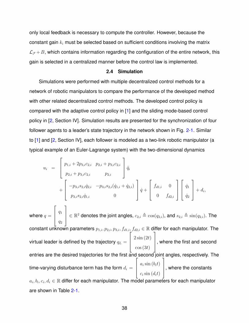
2.4 Simulation
Simulations were performed with multiple decentralized control methods for a
network of robotic manipulators to compare the performance of the developed method
with other related decentralized control methods. The developed control policy is
compared with the adaptive control policy in [1] and the sliding mode-based control
policy in [2, Section IV]. Simulation results are presented for the synchronization of four
follower agents to a leader’s state trajectory in the network shown in Fig. 2-1. Similar
to [1] and [2, Section IV], each follower is modeled as a two-link robotic manipulator (a
typical example of an Euler-Lagrange system) with the two-dimensional dynamics
ui =
p1,i + 2p3,ic2,i p2,i + p3,ic2,i
p2,i + p3,ic2,i p2,i
qi+
−p3,is2,iq2,i −p3,is2,i(q1,i + q2,i)
p3,is2,iq1,i 0
q +
fd1,i 0
0 fd2,i
q1
q2
+ di,
where q =
q1
q2
∈ R2 denotes the joint angles, c2,i , cos(q2,i), and s2,i , sin(q2,i). The
constant unknown parameters p1,i, p2,i, p3,i, fd1,i, fd2,i ∈ R differ for each manipulator. The
virtual leader is defined by the trajectory qL =
2 sin (2t)
cos (3t)
, where the first and second
entries are the desired trajectories for the first and second joint angles, respectively. The
time-varying disturbance term has the form di =
ai sin (bit)
ci sin (dit)
, where the constants
ai, bi, ci, di ∈ R differ for each manipulator. The model parameters for each manipulator
are shown in Table 2-1.
38
The control gains for each method were selected based on convergence rate,
residual error, and magnitude of control authority. The gains were obtained for each
controller by qualitatively determining an appropriate range for each gain and then
running 10,000 simulations with random gain sampling within those ranges in attempt to
minimize
J =4∑i=1
2∑j=1
rms[2,10] (qL,j − qi,j) (2–37)
(with aij = 1 if (j, i) ∈ EF and bi = 4 if (L, i) ∈ EL) while satisfying bounds on the control
input such that the entry-wise inequality uk (t) ≤
500
150
, k = 1, 2, 3, 4, ∀t ∈ [0.2, 10]
is satisfied, where rms[2,10] (·) denotes the root-mean-square (RMS) of the argument’s
sampled trajectory over the time interval [2, 10]. Beginning the RMS error at two seconds
encourages high convergence rate and low residual error, while monitoring the control
input only after 0.2 seconds accommodates for a possibly high initial control input. The
cost function in (2–37) was chosen based on the synchronization goal that ‖qL − qi‖
goes to zero.
Fig. 2-2 and 2-3 demonstrate that asymptotic synchronization of the follower
agents and tracking of the leader trajectory are qualitatively achieved for the developed
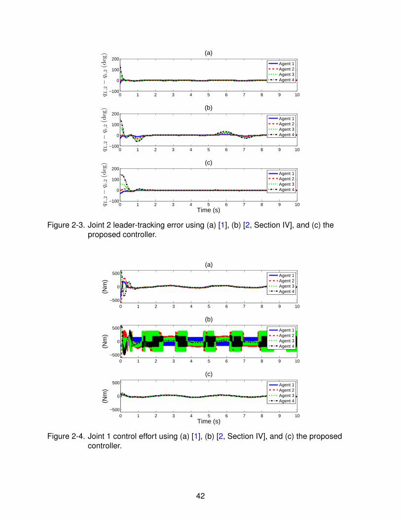
controller, despite the exogenous disturbances. Fig. 2-4 and 2-5 illustrate the effects
of the control methods used to obtain synchronization: the controller in [2, Section IV]
utilizes a high frequency, discontinuous, sliding-mode based control signal, whereas the
developed controller is continuous and exhibits lower frequency content.
As shown in Fig. 2-2 and 2-3, asymptotic synchronization is qualitatively achieved
more slowly for the control method in [2, Section IV], despite the fact that it is based on
sliding-mode control concepts. This is due to the magnitude of the control signal being
produced and the way the simulation trials are vetted. Observe from Fig. 2-4 that the
control effort for [2, Section IV] is near to violating the entry-wise inequality uk (t) ≤
39
500
150
; larger gains lead the control signal to violating this condition. In conclusion, it
qualitatively appears that the control method in [2, Section IV] needs a higher control
magnitude in addition to its high frequency content to achieve synchronization at a
similar rate compared to the developed control method.
As shown in Fig. 2-2 - 2-5, the neural network-based adaptive controller given in [1]
stabilizes the system using a continuous controller which produces a control signal
of moderate magnitude, but maintains a residual error. This behavior agrees with the
theoretical result in [1]: the controller achieves bounded convergence.
Table 2-2 provides a quantitative comparison of the controllers, where J is intro-
duced in (2–37). Compared to the methods in [1] and [2, Section IV], the proposed
controller provides significantly improved tracking performance with a continuous control
signal of a relatively low magnitude.
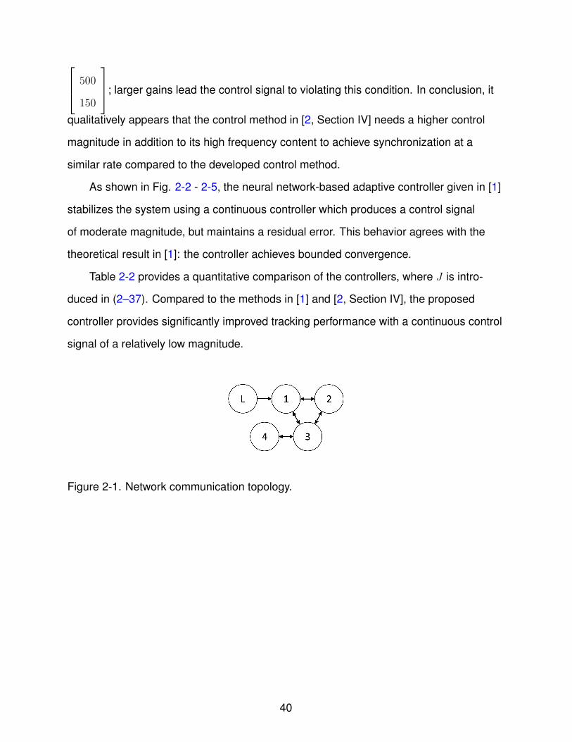
Figure 2-1. Network communication topology.
40
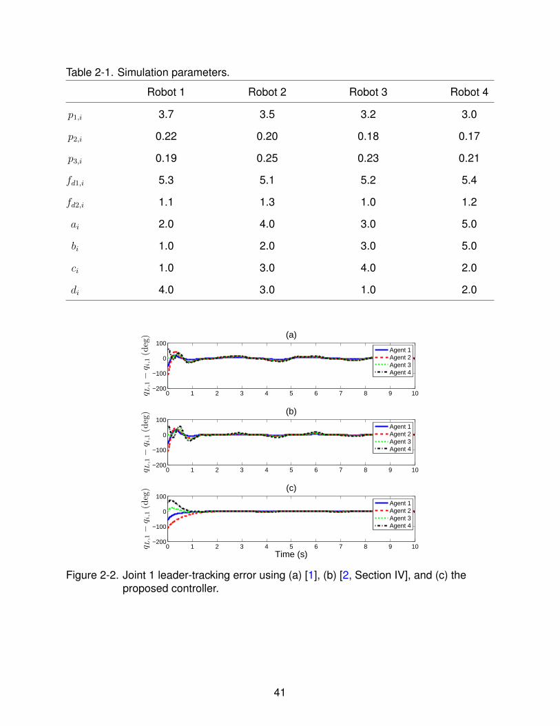
Table 2-1. Simulation parameters.
Robot 1 Robot 2 Robot 3 Robot 4
p1,i 3.7 3.5 3.2 3.0
p2,i 0.22 0.20 0.18 0.17
p3,i 0.19 0.25 0.23 0.21
fd1,i 5.3 5.1 5.2 5.4
fd2,i 1.1 1.3 1.0 1.2
ai 2.0 4.0 3.0 5.0
bi 1.0 2.0 3.0 5.0
ci 1.0 3.0 4.0 2.0
di 4.0 3.0 1.0 2.0
0 1 2 3 4 5 6 7 8 9 10−200
−100
0
100(a)
q L,1−
q i,1(deg)
Agent 1Agent 2Agent 3Agent 4
0 1 2 3 4 5 6 7 8 9 10−200
−100
0
100(b)
q L,1−
q i,1(deg)
Agent 1Agent 2Agent 3Agent 4
0 1 2 3 4 5 6 7 8 9 10−200
−100
0
100(c)
Time (s)
q L,1−
q i,1(deg)
Agent 1Agent 2Agent 3Agent 4
Figure 2-2. Joint 1 leader-tracking error using (a) [1], (b) [2, Section IV], and (c) theproposed controller.
41
0 1 2 3 4 5 6 7 8 9 10−100
0
100
200(a)
q L,2−
q i,2(deg)
Agent 1Agent 2Agent 3Agent 4
0 1 2 3 4 5 6 7 8 9 10−100
0
100
200(b)
q L,2−
q i,2(deg)
Agent 1Agent 2Agent 3Agent 4
0 1 2 3 4 5 6 7 8 9 10−100
0
100
200(c)
Time (s)
q L,2−
q i,2(deg)
Agent 1Agent 2Agent 3Agent 4
Figure 2-3. Joint 2 leader-tracking error using (a) [1], (b) [2, Section IV], and (c) theproposed controller.
0 1 2 3 4 5 6 7 8 9 10−500
0
500
(a)
(Nm
)
Agent 1Agent 2Agent 3Agent 4
0 1 2 3 4 5 6 7 8 9 10−500
0
500
(b)
(Nm
)
Agent 1Agent 2Agent 3Agent 4
0 1 2 3 4 5 6 7 8 9 10−500
0
500
(c)
Time (s)
(Nm
)
Agent 1Agent 2Agent 3Agent 4
Figure 2-4. Joint 1 control effort using (a) [1], (b) [2, Section IV], and (c) the proposedcontroller.
42

0 1 2 3 4 5 6 7 8 9 10
−100
0
100
(a)
(Nm
)
Agent 1Agent 2Agent 3Agent 4
0 1 2 3 4 5 6 7 8 9 10
−100
0
100
(b)(N
m)
Agent 1Agent 2Agent 3Agent 4
0 1 2 3 4 5 6 7 8 9 10
−100
0
100
(c)
Time (s)
(Nm
)
Agent 1Agent 2Agent 3Agent 4
Figure 2-5. Joint 2 control effort using (a) [1], (b) [2, Section IV], and (c) the proposedcontroller.
Table 2-2. Controller performance comparison.
Method maxt∈[0.2,10] maxi∈VF ‖ui‖ (Nm) J
[1] 352 0.638
[2, Section IV] 500 0.569
Proposed 73.4 0.0863
2.5 Extension to Formation Control
2.5.1 Modified Error Signal
Driving the neighborhood-based error signal in (2–5) to zero for each follower
agent provides network synchronization such that the state of every agent converges
to the state of the leader; for example, power networks supported by generators need
to maintain synchronization of the generator phase angles to avoid damage of the
electrical infrastructure system. However, for some applications, it may be desirable to
drive the states of the follower agents to a configuration that is spatially oriented with
43
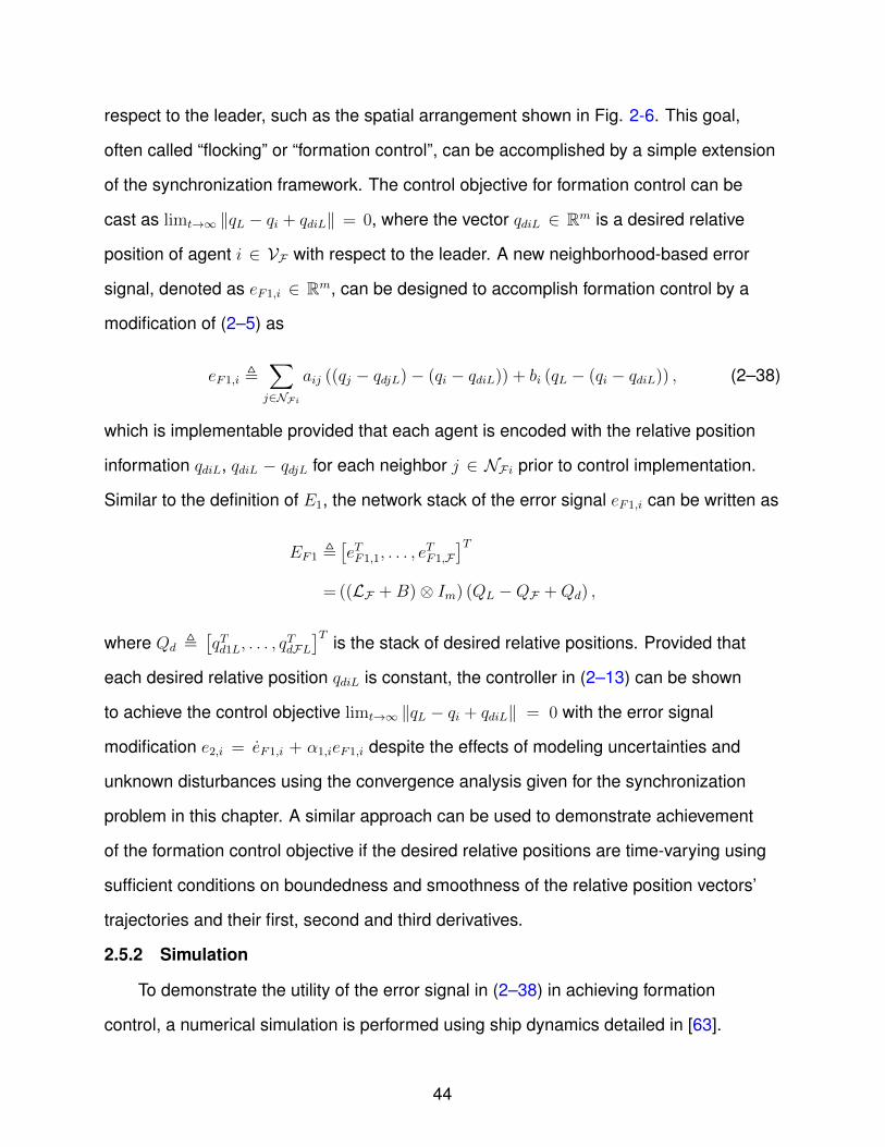
respect to the leader, such as the spatial arrangement shown in Fig. 2-6. This goal,
often called “flocking” or “formation control”, can be accomplished by a simple extension
of the synchronization framework. The control objective for formation control can be
cast as limt→∞ ‖qL − qi + qdiL‖ = 0, where the vector qdiL ∈ Rm is a desired relative
position of agent i ∈ VF with respect to the leader. A new neighborhood-based error
signal, denoted as eF1,i ∈ Rm, can be designed to accomplish formation control by a
modification of (2–5) as
eF1,i ,∑j∈NFi
aij ((qj − qdjL)− (qi − qdiL)) + bi (qL − (qi − qdiL)) , (2–38)
which is implementable provided that each agent is encoded with the relative position
information qdiL, qdiL − qdjL for each neighbor j ∈ NFi prior to control implementation.
Similar to the definition of E1, the network stack of the error signal eF1,i can be written as
EF1 ,[eTF1,1, . . . , e
TF1,F
]T= ((LF +B)⊗ Im) (QL −QF +Qd) ,
where Qd ,[qTd1L, . . . , q
TdFL]T is the stack of desired relative positions. Provided that
each desired relative position qdiL is constant, the controller in (2–13) can be shown
to achieve the control objective limt→∞ ‖qL − qi + qdiL‖ = 0 with the error signal
modification e2,i = eF1,i + α1,ieF1,i despite the effects of modeling uncertainties and
unknown disturbances using the convergence analysis given for the synchronization
problem in this chapter. A similar approach can be used to demonstrate achievement
of the formation control objective if the desired relative positions are time-varying using
sufficient conditions on boundedness and smoothness of the relative position vectors’
trajectories and their first, second and third derivatives.
2.5.2 Simulation
To demonstrate the utility of the error signal in (2–38) in achieving formation
control, a numerical simulation is performed using ship dynamics detailed in [63].
44
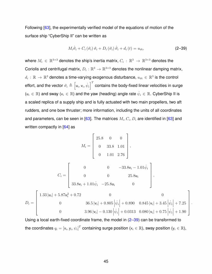
Following [63], the experimentally verified model of the equations of motion of the
surface ship “CyberShip II” can be written as
Miϑi + Ci (ϑi)ϑi +Di (ϑi) ϑi + di (t) = uϑi, (2–39)
where Mi ∈ R3×3 denotes the ship’s inertia matrix, Ci : R3 → R3×3 denotes the
Coriolis and centrifugal matrix, Di : R3 → R3×3 denotes the nonlinear damping matrix,
di : R → R3 denotes a time-varying exogenous disturbance, uϑi ∈ R3 is the control
effort, and the vector ϑi ,[ui, vi, ψi
]Tcontains the body-fixed linear velocities in surge
(ui ∈ R) and sway (vi ∈ R) and the yaw (heading) angle rate ψi ∈ R. CyberShip II is
a scaled replica of a supply ship and is fully actuated with two main propellers, two aft
rudders, and one bow thruster; more information, including the units of all coordinates
and parameters, can be seen in [63]. The matrices Mi, Ci, Di are identified in [63] and
written compactly in [64] as
Mi =
25.8 0 0
0 33.8 1.01
0 1.01 2.76
,
Ci =
0 0 −33.8vi − 1.01ψi
0 0 25.8ui
33.8vi + 1.01ψi −25.8ui 0
,
Di =
1.33 |ui|+ 5.87u2
i + 0.72 0 0
0 36.5 |vi|+ 0.805∣∣∣ψi∣∣∣+ 0.890 0.845 |vi|+ 3.45
∣∣∣ψi∣∣∣+ 7.25
0 3.96 |vi| − 0.130∣∣∣ψi∣∣∣+ 0.0313 0.080 |vi|+ 0.75
∣∣∣ψi∣∣∣+ 1.90
.Using a local earth-fixed coordinate frame, the model in (2–39) can be transformed to
the coordinates qi = [xi, yi, ψi]T containing surge position (xi ∈ R), sway position (yi ∈ R),
45

and yaw angle ψi as
M ′ (qi) q + C ′i (qi, qi) qi +D′i (qi, qi) qi + d′i = u′i (2–40)
with the kinematic transformations
M ′i =J−Ti MiJ
−Ti
C ′i =J−Ti
[Ci −MiJ
−1i Ji
]J−1i
D′i =J−Ti DiJ−1i
d′i =J−Ti di
where u′i ∈ R3 and the rotation matrix J provides the kinematic relationship qi = Ji (qi)ϑi
as
Ji =
cos (ψi) − sin (ψi) 0
sin (ψi) cos (ψi) 0
0 0 1
.Thus, the ship’s dynamics can be transformed to a model with the same structure
as (2–2), where u′i is used to command the formation control in terms of surge, sway
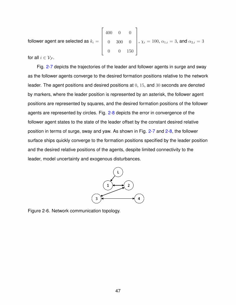
and yaw. The simulation is performed with four follower agents in the communication
topology shown in Fig. 2-6, where each follower agent is modeled with the dynamics
for the ship CyberShip II given in (2–40). Each surface ship is affected by disturbances
(e.g., waves) as d′i = [a1,i sin (t) , a2,i sin (t) , 0]T , where the constants a1, a2 ∈ R are
shown in Table 2-3. The desired formation of the surface ships with respect to the
leader is encoded with the constant vectors qdiL, which are given in Table 2-3. The initial
positions of the follower agents are not coincident with the initial desired positions and
are described in Table 2-3. The initial velocities for each follower agent i ∈ VF are
set as qi (0) = [0, 0, 0]T . The leader trajectory traces an ellipse with the trajectories
uL = 10 cos(
140
(2πt)), vL = 5 sin
(140
(2πt)), ψL = tan−1
(vLuL
). The control gains for each
46
follower agent are selected as ki =
400 0 0
0 300 0
0 0 150
, χi = 100, α1,i = 3, and α2,i = 3
for all i ∈ VF .
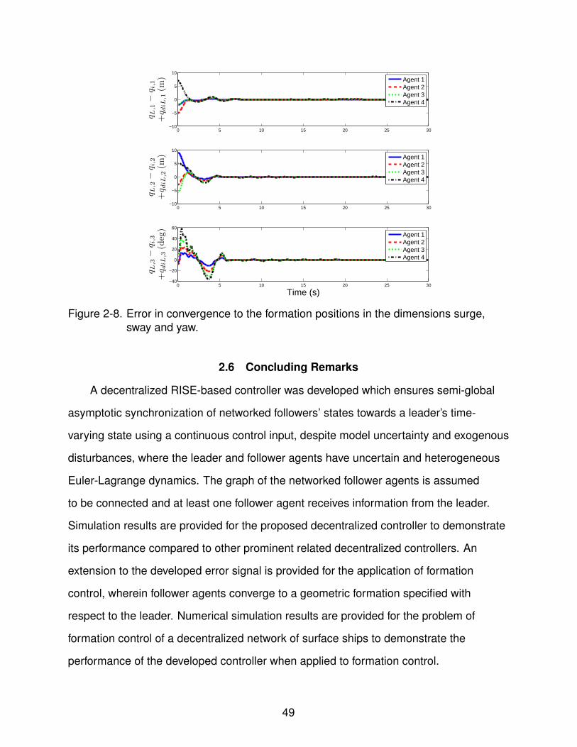
Fig. 2-7 depicts the trajectories of the leader and follower agents in surge and sway
as the follower agents converge to the desired formation positions relative to the network
leader. The agent positions and desired positions at 0, 15, and 30 seconds are denoted
by markers, where the leader position is represented by an asterisk, the follower agent
positions are represented by squares, and the desired formation positions of the follower
agents are represented by circles. Fig. 2-8 depicts the error in convergence of the
follower agent states to the state of the leader offset by the constant desired relative
position in terms of surge, sway and yaw. As shown in Fig. 2-7 and 2-8, the follower
surface ships quickly converge to the formation positions specified by the leader position
and the desired relative positions of the agents, despite limited connectivity to the
leader, model uncertainty and exogenous disturbances.
Figure 2-6. Network communication topology.
47

Table 2-3. Disturbance and formation position parameters.
Robot 1 Robot 2 Robot 3 Robot 4
a1,i 0.5 1.1 0.7 0.2
a2,i 0.9 −0.5 −0.8 0.4
qdiL
−2
−2
0
2
−2
0
−4
−4
0
4
−4
0
qi (0)
10
−11
5.7
17
1
8.6
8
2
−5.7
7
−9
−11
−20 −15 −10 −5 0 5 10 15 20
−15
−10
−5
0
5
10
Surge (m)
Sw
ay (
m)
LeaderRobot 1Robot 2Robot 3Robot 4
Figure 2-7. Agent trajectories in surge and sway.
48
0 5 10 15 20 25 30−10
−5
0
5
10
q L,1−
q i,1
+q d
iL,1(m
)
Agent 1Agent 2Agent 3Agent 4
0 5 10 15 20 25 30−10
−5
0
5
10q L
,2−
q i,2
+q d
iL,2(m
)
Agent 1Agent 2Agent 3Agent 4
0 5 10 15 20 25 30−40
−20
0
20
40
60
Time (s)
q L,3−
q i,3
+q d
iL,3(deg)
Agent 1Agent 2Agent 3Agent 4
Figure 2-8. Error in convergence to the formation positions in the dimensions surge,sway and yaw.
2.6 Concluding Remarks
A decentralized RISE-based controller was developed which ensures semi-global
asymptotic synchronization of networked followers’ states towards a leader’s time-
varying state using a continuous control input, despite model uncertainty and exogenous
disturbances, where the leader and follower agents have uncertain and heterogeneous
Euler-Lagrange dynamics. The graph of the networked follower agents is assumed
to be connected and at least one follower agent receives information from the leader.
Simulation results are provided for the proposed decentralized controller to demonstrate
its performance compared to other prominent related decentralized controllers. An
extension to the developed error signal is provided for the application of formation
control, wherein follower agents converge to a geometric formation specified with
respect to the leader. Numerical simulation results are provided for the problem of
formation control of a decentralized network of surface ships to demonstrate the
performance of the developed controller when applied to formation control.
49
CHAPTER 3ROBUST CONTAINMENT CONTROL IN A LEADER-FOLLOWER NETWORK OF
UNCERTAIN EULER-LAGRANGE SYSTEMS
The previous chapter presented a controller development for the asymptotic
synchronization of a network of follower agents to the trajectory of a single leader.
This chapter extends the decentralized controller for single-leader synchronization to
the problem of tracking multiple leaders by a network of follower agents. Tracking of
multiple leaders is generally referred to as containment control, wherein follower agents
can communicate with multiple leaders; for example, containment control is useful in
applications where a team of autonomous vehicles is directed by multiple pilots or for
networks of autonomous systems where only a subset of the systems is equipped with
expensive sensing hardware. The typical objective of containment control is to drive
the states of the follower agents to the convex hull of the leaders’ states, where each
follower agents’ trajectory converges to a linear combination of the leaders’ trajectories
which depends on the structure of the follower network, leader connections, and the
weights in the decentralized error signals. This result is facilitated by a lemma which
relates a neighborhood-based error signal to containment of the follower agents within
the dynamic convex hull spanned by the leaders’ states.
3.1 Problem Formulation
3.1.1 Notation for a Multi-Leader Network
Some additional notation is introduced to facilitate the description of multiple
leaders’ interaction within a network. Consider a network of L ∈ Z>0 leader agents
and F ∈ Z>0 follower agents. Communication of the follower agents is described with
a fixed undirected graph, GF = {VF , EF}, where VF , {L+ 1, . . . , L+ F} is the set of
follower nodes and EF ⊆ VF × VF is the corresponding edge set. An undirected edge
(j, i) (and also (i, j)) is an element of EF if agents i, j ∈ VF communicate information
with each other; without loss of generality, the graph is considered to be simple, i.e.,
(i, i) /∈ EF ∀i ∈ VF . The follower agent neighbor set NFi , {j ∈ VF | (j, i) ∈ EF} is the
50
set of follower agents that transmit information to agent i. The connections in GF are
succinctly described with the adjacency matrix AF = [aij] ∈ RF×F , where aij > 0 if
(j, i) ∈ EF and aij = 0 otherwise. The Laplacian matrix LF = [pij] ∈ RF×F associated
with graph GF is constructed such that pii =∑
j∈NFi aij and pij = −aij if i 6= j. The
directed graph G = {VF ∪ VL, EF ∪ EL} containing both the leader and follower agents is
a supergraph of GF constructed by appending an edge (l, i) ∈ EL to GF if leader agent
l ∈ VL communicates information to follower agent i ∈ VF , where VL , {1, . . . , L} is the
leader node set and EL ⊆ VL × VF is the set of leader-follower edges. The adjacency
matrix A = [aij] ∈ R(L+F)×(L+F) for graph G is similarly defined such that aij > 0 if
(j, i) ∈ EF ∪ EL and aij = 0 otherwise. Let the diagonal leader-connectivity matrix
B = [bij] ∈ RF×F be defined such that bii =∑
l∈VL ail. The Laplacian matrix for graph G
can be constructed similarly to LF and can be represented as L =
0L×L 0L×F
LL LF +B
,
where LL ∈ RF×L.
3.1.2 Dynamic Models and Properties
The dynamics of each follower agent i ∈ VF are described by the nonidentical
Euler-Lagrange equations of motion
Mi (qi) qi + Ci (qi, qi) qi + Fi (qi) +Gi (qi) + di = ui, (3–1)
where qi ∈ Rm is the generalized configuration coordinate, Mi : Rm → Rm×m is the
inertia matrix, Ci : Rm × Rm → Rm×m is the Coriolis/centrifugal matrix, Fi : Rm → Rm
represents friction, Gi : Rm → Rm represents gravitational effects, ui ∈ Rm represents
the vector of control inputs, and di : R≥0 → Rm is a time-varying nonlinear exogenous
disturbance. Functional dependency will be omitted in the remainder of the chapter
where the meaning is clear from context. The following assumption is characteristic of
physical systems with dynamics described by Euler-Lagrange equations of motion.
51
Assumption 3.1. For each follower agent i ∈ VF , the inertia matrix is positive definite
and symmetric, and there exist positive constants m, m ∈ R such that the inertia matrix
satisfies the inequalities m ‖ξ‖2 ≤ ξTMi (ψ) ξ ≤ m ‖ξ‖2 for all ξ, ψ ∈ Rm and i ∈ VF .
The following assumptions concerning the smoothness of dynamics and network
connectivity are used in the subsequent controller performance analysis.
Assumption 3.2. [52] For each follower agent i ∈ VF , the functions Mi, Ci, Fi, Gi are
second order differentiable such that the second time derivative is bounded provided
q(k)i ∈ L∞, k = 0, . . . , 3.
Assumption 3.3. [51] For each follower agent i ∈ VF , the time-varing disturbance term
is sufficiently smooth such that it and its first two time derivatives, di, di, di, are bounded
by known1 constants.
Assumption 3.4. Each time-varying leader configuration coordinate, ql : R≥0 → Rm
(l ∈ VL), is sufficiently smooth such that ql ∈ C2; additionally, each leader configuration
coordinate and its first two time derivatives are bounded such that ql, ql, ql ∈ L∞.
Assumption 3.5. For each follower agent i ∈ VF , there exists a directed path from a
leader l ∈ VL to i.
Note that, similar to Chapter 2, the matrix LF + B is positive definite by Assumption
3.5 and [18, Lemma 4.1]. For convenience, the follower agents’ dynamics are stacked
as
MQF + CQF + F +G+ d = u, (3–2)
where M , diag (ML+1, . . . ,ML+F) ∈ RFm×Fm, QF ,
[qTL+1, . . . , qTL+F
]T∈
RFm, C , diag (CL+1, . . . , CL+F) ∈ RFm×Fm, F ,
[F TL+1, . . . , F T
L+F
]T∈ RFm,
1 Following the developments in [53] and [54], Assumption 3.3 can be relaxed suchthat the bounding constants can be unknown.
52
G ,
[GTL+1, . . . , GT
L+F
]T∈ RFm, d ,
[dTL+1, . . . , dTL+F
]T∈ RFm, and
u ,
[uTL+1, . . . , uTL+F
]T∈ RFm.
3.1.3 Control Objective
The objective is to design a continuous controller for the follower agent dynamics in
(3–1) which drives the states of all follower agents to the (possibly time-varying) convex
hull spanned by the leader agents’ states despite exogenous input disturbances and
modeling uncertainties. Furthermore, only the configuration coordinate and its first time
derivative are assumed to be measurable for the leader and follower agents. An error
signal, e1,i ∈ Rm (i ∈ VF), is developed to quantify the neighborhood tracking error as
e1,i ,∑
j∈VF∪VL
aij (qi − qj) , (3–3)
which includes the state difference between neighboring follower agents and neighbor-
ing leader agents, if those connections exist. Note that there is no restriction on an edge
weight aij for an existing connection (j, i) ∈ E other than that the weight is positive and
aij = aji ∀i, j ∈ VF . Therefore, the control can emphasize a connection (j, i) by increas-
ing aij if it is desired for agent i ∈ VF to maintain close similarity to agent j ∈ VF ∪ VL .
An auxiliary tracking error, e2,i ∈ Rm, is designed as
e2,i , e1,i + α1,ie1,i,
where α1,i ∈ R>0 is a constant gain. By stacking the follower agents’ error signals e1,i
and e2,i as E1 ,[eT1,L+1, . . . , e
T1,L+F
]T ∈ RFm and E2 ,[eT2,L+1, . . . , e
T2,L+F
]T ∈ RFm, the
network error dynamics can be written as
E1 = ((LF +B)⊗ Im)QF + (LL ⊗ Im)QL, (3–4)
E2 = E1 + Λ1E1, (3–5)
53

where QL ,
[qT1 , . . . , qTL
]T∈ RLm is the stack of leader agent states, and
Λ1 , diag (α1,L+1, . . . , α1,L+F) ⊗ Im ∈ RFm×Fm is a diagonal matrix of gains. An auxiliary
error signal, R ∈ RFm, is designed as
R ,((LF +B)−1 ⊗ Im
) (E2 + Λ2E2
), (3–6)
where Λ2 , diag (α2,L+1, . . . , α2,L+F) ⊗ Im ∈ RFm×Fm is a diagonal matrix containing the
gains α2,i ∈ R>0. The auxiliary error signal R is not used in the subsequently designed
controller since it depends on the second derivative of the configuration coordinate and
is only introduced to facilitate an expression for the closed-loop error system.
Similar to [24], the error system in (3–3) is designed such that ‖E1‖ → 0 implies
that the Euclidean distance from qi to the convex hull formed by the leader agents also
asymptotically converges to zero for all i ∈ VF . This implication is stated in the following
lemma, which is used in the subsequent development.
Lemma 3.1. If Assumption 3.5 is satisfied, then ‖E1‖ → 0 implies that
d (qi,Conv {ql | l ∈ VL})→ 0 ∀i ∈ VF ,
where Conv {·} denotes the convex hull of the set of points in its argument and the
distance d (p, S) between a point p and a set S is defined as infs∈S ‖p− s‖ for all p ∈ Rn
and S ⊂ Rn.
Proof. See Appendix B.
3.2 Controller Development
An open-loop error system is designed by pre-multiplying the auxiliary tracking error
R in (3–6) by M and using (3–2), (3–4) and (3–5) as
MR = u− d+ S1 + S2, (3–7)
54

where the functions S1 : Π7k=1RFm → RFm and S2Π3
k=1RFm → RFm are defined as
S1 ,M (QF)((LF +B)−1 ⊗ Im
) ((Λ1 + Λ2)E2 − Λ2
1E1
)− C
(QF , QF
)QF
− F(QF
)−G (QF) +M (QF)
((LF +B)−1 LL ⊗ Im
)QL
+ F(((
(LF +B)−1 LL)⊗ Im
)QL
)+G
((((LF +B)−1 LL
)⊗ Im
)QL
)+ C
((((LF +B)−1 LL
)⊗ Im
)QL,
(((LF +B)−1 LL
)⊗ Im
)QL
)·((
(LF +B)−1 LL)⊗ Im
)QL
−M(((
(LF +B)−1 LL)⊗ Im
)QL
) ((LF +B)−1 LL ⊗ Im
)QL,
S2 ,− C(((
(LF +B)−1 LL)⊗ Im
)QL,
(((LF +B)−1 LL
)⊗ Im
)QL
)×((
(LF +B)−1 LL)⊗ Im
)QL − F
((((LF +B)−1 LL
)⊗ Im
)QL
)−G
((((LF +B)−1 LL
)⊗ Im
)QL
)+M
((((LF +B)−1 LL
)⊗ Im
)QL
) ((LF +B)−1 LL ⊗ Im
)QL.
Terms in (3–7) are organized so that, after a Mean Value Theorem-based approach
(cf. [58, Lemma 5]), ‖S1‖ can be upper-bounded by a function of the errors sig-
nals E1, E2, R and ‖S2‖ can be upper-bounded by a constant. Note that the term
M (QF)((LF +B)−1 ⊗ Im
)((Λ1 + Λ2)E2 − Λ2
1E1) can be upper-bounded by a function
of the error signals using a Mean Value Theorem-based approach after adding and
subtracting the term
M(((
(LF +B)−1 LL)⊗ Im
)QL
) ((LF +B)−1 ⊗ Im
) ((Λ1 + Λ2)E2 − Λ2
1E1
)within S1.
The developed robust decentralized controller for follower agent i ∈ VF is designed
as
ui =∑j∈NFi
aij ((ks,j + Im) e2,j − (ks,i + Im) e2,i)− bii (ks,i + Im) e2,i + νi, (3–8)
55
where the function νi : Π|NFi|+1j=1 Rm → Rm is the generalized solution to the differential
equation
νi ,∑j∈NFi
aij ((ks,j + Im)α2,je2,j − (ks,i + Im)α2,ie2,i)
+∑j∈NFi
aij (χj sgn (e2,j)− χi sgn (e2,i))− (ks,i + Im) biiα2,ie2,i − biiχi sgn (e2,i) (3–9)
with νi (0) = νi0 ∈ Rm as a user-specified initial condition, where ks,i ∈ Rm×m is a
constant positive definite gain matrix, χi ∈ Rm×m is a constant diagonal positive definite
gain matrix, and the function sgn (·) is defined for all ξ =
[ξ1, . . . , ξv
]T∈ Rv as
sgn (ξ) ,
[sgn (ξ1) , . . . , sgn (ξv)
]T. Note that the controller in (3–8) is continuous,
only relies on the configuration coordinate and its first derivative, and is decentralized in
communication: agent i requires its own error signal and the error signals of neighbors
j ∈ NFi. The use of neighbors’ error signals in the control law provides cooperation
among the follower agents. Assuming that a neighbor’s state can be sensed, then
only one-hop communication is necessary to compute the control authority in (3–8). In
(3–8) and (3–9), the terms multiplied by the gain ks,i provide proportional and derivative
feedback and the terms multiplied by the gain χi provide robust feedback which is used
to reject the unknown time-varying disturbances, as shown in the following convergence
analysis. Note that a strategy involving additive gradient-based control terms, such as
that in [65], can be used if collision avoidance is necessary for the control objective.
After taking the time-derivative of (3–7), the closed-loop error system can be
represented as
MR =− ((LF +B)⊗ Im) (Ks + IFm)(E2 + Λ2E2
)− ((LF +B)⊗ Im) β sgn (E2)
+ N + ((LF +B)⊗ Im)Nd − ((LF +B)⊗ Im)E2 −1
2MR, (3–10)
56
where the first two terms are contributions from the derivative of the stack of follower
agents’ control inputs
u = ((LF +B)⊗ Im) (Ks + IFm)(E2 + Λ2E2
)− ((LF +B)⊗ Im) β sgn (E2) ,
Ks , diag (ks,L+1, . . . , ks,L+F) ∈ RFm×Fm is a block diagonal gain matrix, β ,
diag (χL+1, . . . , χL+F) ∈ RFm×Fm is a diagonal gain matrix, and the unknown auxil-
iary functions N and Nd are defined as
N , S1 + ((LF +B)⊗ Im)E2 −1
2MR, (3–11)
Nd ,((LF +B)−1 ⊗ Im
) (d+ S2
). (3–12)
Terms in N are segregated such that after taking advantage of the expressions QF =((LF +B)−1 ⊗ Im
)E1 −
((LF +B)−1 ⊗ Im
)(LL ⊗ Im)QL, E1 = E2 − Λ1E1, and
E2 = ((LF +B)⊗ Im)R − Λ2E2, Assumptions 3.2 and 3.4, and a Mean Value Theorem-
based approach (cf. [58, Lemma 5]), (3–11) can be upper-bounded by∥∥∥N∥∥∥ ≤ ρ (‖Z‖) ‖Z‖ , (3–13)
where Z ∈ R3Fm is the composite error vector defined as Z ,
[ET
1 ET2 RT
]T, and
ρ : R≥0 → R≥0 is a strictly increasing, radially unbounded function. Moreover, other
terms in (3–10) are segregated in the function Nd such that it and its first derivative can
be upper-bounded such that, for all k ∈ {1, . . . ,Fm},
supt∈[0,∞)
|Nd|k ≤ δa,k,
supt∈[0,∞)
∣∣∣Nd
∣∣∣k≤ δb,k,
after using Assumptions 3.3 and 3.4, where |·|k denotes the absolute value of the
kth component of the vector argument, and δa,k, δb,k ∈ R>0 are constant bounds. In
the subsequent convergence analysis, the terms in Nd and Nd are compensated by
57
using the signum feedback terms in (3–9). For clarity in the following section, let the
vectors ∆a,i,∆b,i ∈ Rm be defined such that ∆a,i ,
[δa,m(i−1)+1 . . . , δa,m(i−1)+m
]Tand ∆b,i ,
[δb,m(i−1)+1 . . . , δb,m(i−1)+m
]T, which represent the contribution of the
disturbance terms for each agent.
3.3 Convergence Analysis
An auxiliary function P : RFm × RFm × R≥0 → R is included in the subsequently
defined candidate Lyapunov function so that sufficient gain conditions may be obtained
for the compensation of the bounded disturbance terms in Nd. Let P be defined as the
generalized solution to the differential equation
P = −(E2 + Λ2E2
)T(Nd − β sgn (E2)) ,
P (0) =Fm∑k=1
βk,k |E2 (0)|k − ET2 (0)Nd (0) , (3–14)
where βk,k denotes the kth diagonal entry of the diagonal gain matrix β. Provided the
sufficient gain condition in (3–18) is satisfied, then P ≥ 0 for all t ∈ [0,∞) (see Appendix
A).
Remark 3.1. Because the closed-loop error system in (3–10) and the derivative of the
signal P in (3–14) are discontinuous, the existence of Filippov solutions in the given
differential equations is addressed before the Lyapunov-based convergence analysis
is presented. Consider the composite vector η ,
[ZT , νTL+1, . . . , νTL+F ,
√P
]T∈
R4Fm+1, composed of the stacked error signals, the signal contributing discontinuities
to the derivative of the developed controller, and the aforementioned auxiliary signal P .
Existence of Filippov solutions for the closed-loop dynamical system η = K [h1] (η, t) can
be established, where h1 : R4Fm+1 × R≥0 → R4Fm+1 is a function defined as the RHS of
η and K [h1] (%, t) , ∩δ>0 ∩µ(Sm)=0 coh1 (Bδ (%) \ Sm, t), where δ ∈ R, ∩µ(Sm)=0 denotes
the intersection over the sets Sm of Lebesgue measure zero, co denotes convex closure,
58
and Bδ (%) ,{σ ∈ R4Fm+1 | ‖%− σ‖ < δ
}, where σ, % ∈ R4Fm+1 are used as dummy
variables [59–61].
Let the auxiliary gain constant Φ ∈ R be defined as
Φ , min
{mini∈VF
α1,i −1
2,mini∈VF
α2,i −1
2, λ((LF +B)2)} .
A continuously differentiable, positive definite candidate Lyapunov function VL : D → R is
defined as
VL (y, t) ,1
2ET
1 E1 +1
2ET
2 E2 +1
2RTM (t)R + P, (3–15)
where the composite vector y ∈ R3Fm+1 is defined as y ,
[ZT
√P
]T, D is defined as
the open and connected set
D ,{σ ∈ R3Fm+1 | ‖σ‖
< inf(ρ−1
([2√
Φλ (((LF +B)⊗ Im)Ks ((LF +B)⊗ Im))),∞))}
,
and ρ−1 (·) denotes the inverse mapping of a set argument. To facilitate the description
of the semi-global property of the following Lyapunov-based convergence analysis, the
set of stabilizing initial conditions SD ⊂ D is defined as
SD ,
{σ ∈ D | ‖σ‖
<
√λ1
λ2
inf(ρ−1([
2√
Φλ (((LF +B)⊗ Im)Ks ((LF +B)⊗ Im))),∞))}
.
Due to the construction of VL in (3–15), VL satisfies the inequalities
λ1 ‖y‖2 ≤ VL (y, t) ≤ λ2 ‖y‖2 ∀t ∈ [0,∞) (3–16)
via Assumption 3.1, where λ1, λ2 ∈ R>0 are constants defined as λ1 , 12
min{
1,minj∈VF mj
}and λ2 , max
{1, 1
2maxj∈VF mj
}. The following theorem describes the performance of
the networked dynamical systems through the use of the Lyapunov function candidate in
(3–15).
59

Theorem 3.1. For every follower agent i ∈ VF , the decentralized controller in (3–8)
guarantees that all signals are bounded under closed-loop control and that containment
control is semi-globally achieved in the sense that d (qi,Conv {ql | l ∈ VL}) → 0 as
t → ∞, provided that the gains ks,i are selected sufficiently large such that the initial
condition y (0) lies within the set of stabilizing initial conditions SD, Assumptions 3.1-
3.5 are satisfied, and the gains α1,i, α2,i, χi are selected according to the sufficient
conditions
α1,i >1
2, α2,i >
1
2, (3–17)
λ (χi) > ‖∆a,i‖∞ +1
α2,i
‖∆b,i‖∞ (3–18)
for all i ∈ VF .
Proof. Using Filippov’s framework, a Filippov solution can be established for the closed-
loop system y = h2 (y, t), where h2 : R3Fm+1 × R≥0 → R3Fm+1 denotes the RHS of
the derivative of the closed-loop error signals and P . Accordingly, the time derivative of
(3–15) exists a.e. on the time domain [0,∞) and VLa.e.∈ ˙VL, where
˙VL = ∩ξ∈∂VL(y,t)ξTK[ET
1 ET2 RT 1
2P−
12 P 1
]T, (3–19)
where ∂VL is the generalized gradient of VL and the entry 1 in (3–19) accommodates
for the expression of M as time-dependent in (3–15). Because VL (y, t) is continuously
differentiable,˙VL ⊆ ∇VLK
[ET
1 ET2 RT 1
2P−
12 P 1
]T, (3–20)
where ∇VL ,
[ET
1 ET2 RTM 2P
12
12RTM (t)R
]. After using the calculus for K [·]
from [60] and substituting expressions from (3–5), (3–6), (3–10) and (3–14), (3–20) may
60
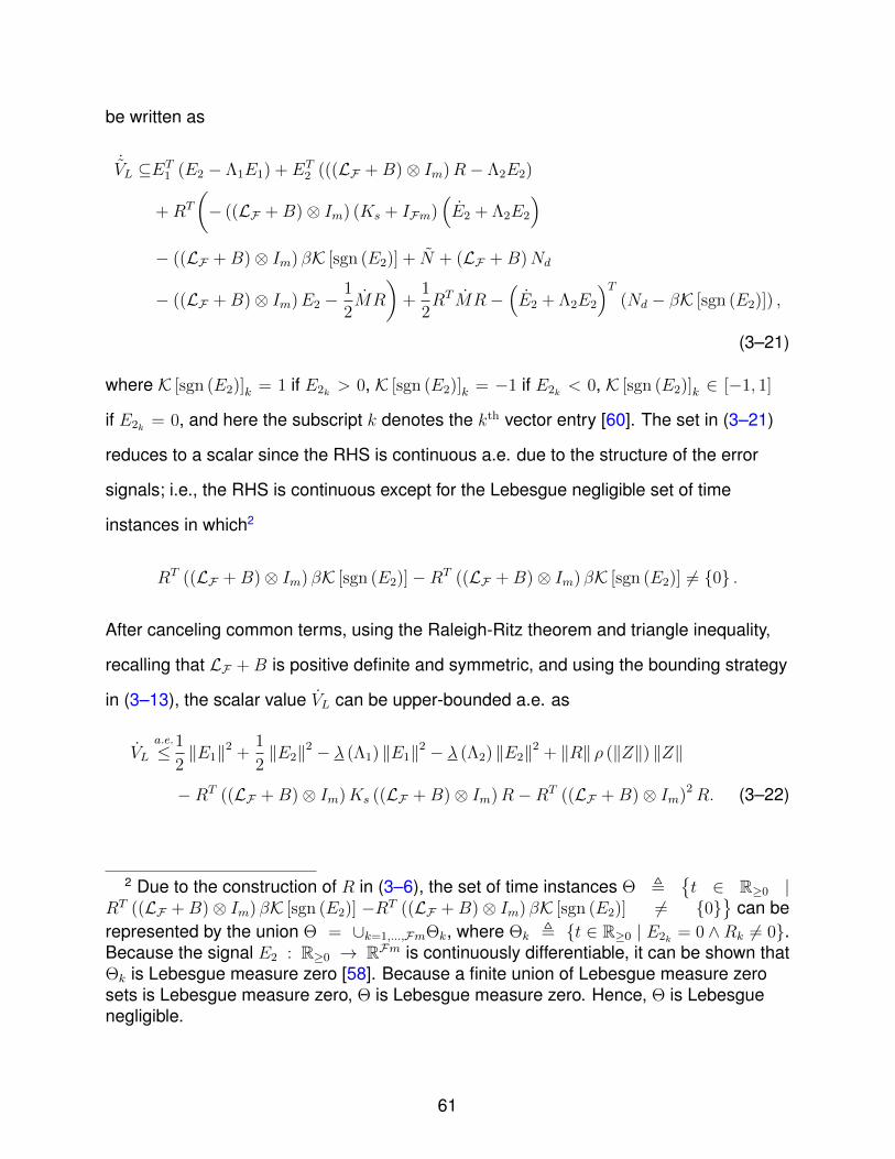
be written as
˙VL ⊆ET1 (E2 − Λ1E1) + ET
2 (((LF +B)⊗ Im)R− Λ2E2)
+RT
(− ((LF +B)⊗ Im) (Ks + IFm)
(E2 + Λ2E2
)− ((LF +B)⊗ Im) βK [sgn (E2)] + N + (LF +B)Nd
− ((LF +B)⊗ Im)E2 −1
2MR
)+
1
2RTMR−
(E2 + Λ2E2
)T(Nd − βK [sgn (E2)]) ,
(3–21)
where K [sgn (E2)]k = 1 if E2k > 0, K [sgn (E2)]k = −1 if E2k < 0, K [sgn (E2)]k ∈ [−1, 1]
if E2k = 0, and here the subscript k denotes the kth vector entry [60]. The set in (3–21)
reduces to a scalar since the RHS is continuous a.e. due to the structure of the error
signals; i.e., the RHS is continuous except for the Lebesgue negligible set of time
instances in which2
RT ((LF +B)⊗ Im) βK [sgn (E2)]−RT ((LF +B)⊗ Im) βK [sgn (E2)] 6= {0} .
After canceling common terms, using the Raleigh-Ritz theorem and triangle inequality,
recalling that LF + B is positive definite and symmetric, and using the bounding strategy
in (3–13), the scalar value VL can be upper-bounded a.e. as
VLa.e.
≤ 1
2‖E1‖2 +
1
2‖E2‖2 − λ (Λ1) ‖E1‖2 − λ (Λ2) ‖E2‖2 + ‖R‖ ρ (‖Z‖) ‖Z‖
−RT ((LF +B)⊗ Im)Ks ((LF +B)⊗ Im)R−RT ((LF +B)⊗ Im)2R. (3–22)
2 Due to the construction of R in (3–6), the set of time instances Θ ,{t ∈ R≥0 |
RT ((LF +B)⊗ Im) βK [sgn (E2)] −RT ((LF +B)⊗ Im) βK [sgn (E2)] 6= {0}}
can berepresented by the union Θ = ∪k=1,...,FmΘk, where Θk , {t ∈ R≥0 | E2k = 0 ∧Rk 6= 0}.Because the signal E2 : R≥0 → RFm is continuously differentiable, it can be shown thatΘk is Lebesgue measure zero [58]. Because a finite union of Lebesgue measure zerosets is Lebesgue measure zero, Θ is Lebesgue measure zero. Hence, Θ is Lebesguenegligible.
61

Using the definition of the auxiliary gain constant Φ, which is positive given the sufficient
gain conditions in (3–17) and the positive definite property of LF + B (note that the
product ((LF +B)⊗ Im)2 is positive definite since LF + B is positive definite and
symmetric), (3–22) is rewritten as
VLa.e.
≤ −Φ ‖Z‖2 − λ (((LF +B)⊗ Im)Ks ((LF +B)⊗ Im)) ‖R‖2 + ‖R‖ ρ (‖Z‖) ‖Z‖ ,
where the product ((LF +B)⊗ Im)Ks ((LF +B)⊗ Im) is positive definite since Ks is
positive definite and LF + B is positive definite and symmetric. After completing the
squares, VL is again upper-bounded a.e. by
VLa.e.
≤ −(
Φ− ρ2 (‖Z‖)4λ (((LF +B)⊗ Im)Ks ((LF +B)⊗ Im))
)‖Z‖2 .
Provided the gains ks,i are selected such that the respective minimum eigenvalues are
sufficiently large such that y (0) ∈ SD, there exists a constant c ∈ R>0 such that
VLa.e.
≤ −c ‖Z‖2 (3–23)
for all y ∈ D. Thus, the inequalities in (3–16) and (3–23) show that VL ∈ L∞ and
therefore E1, E2, R ∈ L∞. A simple analysis of the closed-loop error system shows that
the remaining signals are also bounded. Furthermore, from (3–23), [61, Corollary 1] can
be used to show c ‖Z‖2 → 0 as t → ∞ for all y (0) ∈ SD. Because the vector Z contains
the vector E1, ‖E1‖ → 0 as t → 0. By Lemma 3.1, d (qi,Conv {ql | l ∈ VL}) → 0 ∀i ∈ VF ,
i.e., each follower agent’s state converges to the convex hull spanned by the leaders’
states.
Note that the controller in (3–8) is decentralized in communication; however,
because the stabilizing set of initial conditions SD depends on the graph dependent
matrix LF + B, the gains ks,i must be selected in a centralized manner before execution
of the control. However, the set SD can be made arbitrarily large to include any initial
62

condition y (0) by increasing the minimum eigenvalues of the gains ks,i to increase the
minimum eigenvalue of the matrix ((LF +B)⊗ Im)Ks ((LF +B)⊗ Im).
3.4 Simulation
To demonstrate the robustness of the developed approach in performing con-
tainment control of follower agents with respect to a set of leader agents, numerical
simulations are performed for a group of AUVs conducting surveillance. Each follower
agent is modeled as a conventional, slender-bodied, fully actuated AUV with nonlinear
dynamics as described in [66] (see [67] for more information on AUV dynamics). The
state of each AUV is composed of surge (x), sway (y), heave (z), roll (φ), pitch (θ), and
yaw (ψ). Actuation of the AUV is modeled by three independent forces acting at the
center of mass of the vehicle and three independent moments which can be produced
with a given thruster configuration and an appropriate thruster mapping algorithm, such
as that described in [68].
Four leader agents are used to direct five follower agents such that the fol-
lower agents’ states converge to the convex hull formed by the leaders’ time-varying
states, which have initial positions shown in Table 3-1, identical initial velocities of
[0.2 m/s, 0 m/s, 0.05 m/s, 0 rad/s, 0 rad/s,−0.1 rad/s]T , and identical accelerations of
[−0.02 sin (0.1t) ,−0.02 cos (0.1t) , 0]T m/s2 in surge, sway and heave, respectively,
such that the leaders form an inclined rectangle which translates in a helical trajec-
tory. The follower AUVs have initial positions shown in Table 3-2 and identical initial
velocities of [2 m/s, 0 m/s, 0 m/s, 0 rad/s, 0 rad/s, 0 rad/s]T . All leader and follower
agents have initial roll, pitch and yaw of 0 rad. The network topology is shown in
Fig. 3-1. As in [69], the external disturbances for the follower AUVs are modeled as
[ui sin (0.5t) , 0.5vi sin (2.5t) , 0.2wi rand]T N in surge, sway and heave, respectively, and
0 Nm in roll, pitch and yaw, where ui, vi, wi ∈ R represent the linear velocities in surge,
sway and heave, respectively, of the ith follower agent, and rand ∈ [−1, 1] is a uniformly
63
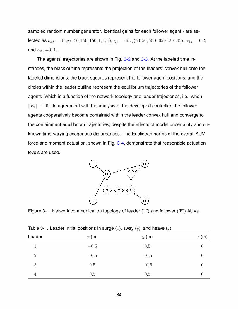
sampled random number generator. Identical gains for each follower agent i are se-
lected as ks,i = diag (150, 150, 150, 1, 1, 1), χi = diag (50, 50, 50, 0.05, 0.2, 0.05), α1,i = 0.2,
and α2,i = 0.1.
The agents’ trajectories are shown in Fig. 3-2 and 3-3. At the labeled time in-
stances, the black outline represents the projection of the leaders’ convex hull onto the
labeled dimensions, the black squares represent the follower agent positions, and the
circles within the leader outline represent the equilibrium trajectories of the follower
agents (which is a function of the network topology and leader trajectories, i.e., when
‖E1‖ ≡ 0). In agreement with the analysis of the developed controller, the follower
agents cooperatively become contained within the leader convex hull and converge to
the containment equilibrium trajectories, despite the effects of model uncertainty and un-
known time-varying exogenous disturbances. The Euclidean norms of the overall AUV
force and moment actuation, shown in Fig. 3-4, demonstrate that reasonable actuation
levels are used.
Figure 3-1. Network communication topology of leader (“L”) and follower (“F”) AUVs.
Table 3-1. Leader initial positions in surge (x), sway (y), and heave (z).
Leader x (m) y (m) z (m)
1 −0.5 0.5 0
2 −0.5 −0.5 0
3 0.5 −0.5 0
4 0.5 0.5 0
64
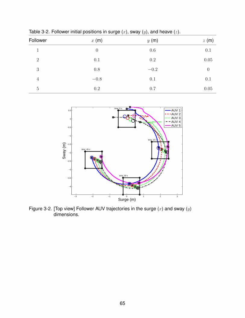
Table 3-2. Follower initial positions in surge (x), sway (y), and heave (z).
Follower x (m) y (m) z (m)
1 0 0.6 0.1
2 0.1 0.2 0.05
3 0.8 −0.2 0
4 −0.8 0.1 0.1
5 0.2 0.7 0.05
−3 −2 −1 0 1 2 3
−4
−3.5
−3
−2.5
−2
−1.5
−1
−0.5
0
0.5time: 0 s
time: 15 s
time: 30 s
time: 45 s
Surge (m)
Sw
ay (
m)
AUV 1AUV 2AUV 3AUV 4AUV 5
Figure 3-2. [Top view] Follower AUV trajectories in the surge (x) and sway (y)dimensions.
65

−2 −1.5 −1 −0.5 0 0.5 1 1.5 2
0
0.5
1
1.5
2
2.5
3
3.5
time: 0 s
time: 15 s
time: 30 s
time: 45 s
Surge (m)
Hea
ve (
m)
AUV 1AUV 2AUV 3AUV 4AUV 5
Figure 3-3. [Front view] Follower AUV trajectories in the surge (x) and heave (z)dimensions.
0 5 10 15 20 25 30 35 40 450
20
40
60
80
100
Time (s)
Ove
rall
forc
e no
rm (
N)
AUV 1AUV 2AUV 3AUV 4AUV 5
0 5 10 15 20 25 30 35 40 450
1
2
3
4
5
Time (s)Ove
rall
mom
ent n
orm
(N
m)
AUV 1AUV 2AUV 3AUV 4AUV 5
Figure 3-4. Euclidean norms of the follower AUV control efforts.
66
3.5 Concluding Remarks
A decentralized controller was developed for cooperative containment control
of autonomous networked follower agents with a set of network leaders, which is a
generalization of the popular single leader-follower network. The developed continuous
controller provides robustness to input disturbances and uncertain, nonlinear Euler-
Lagrange dynamics such that the state of each follower agent asymptotically converges
to the convex hull spanned by the leaders’ time-varying states for an arbitrary number
of leaders. Some notable assumptions are that the agents’ dynamics and disturbances
are smooth, the graph containing the follower agents is connected and at least one
follower agent is connected to at least one leader. Simulation results are provided to
demonstrate the disturbance rejection capability of the developed controller.
67
CHAPTER 4SYNCHRONIZATION OF UNCERTAIN EULER-LAGRANGE SYSTEMS WITH
UNCERTAIN TIME-VARYING COMMUNICATION DELAYS
The work in the previous chapters is developed using a model which assumes that
network neighbors communicate instantaneously. Efforts in this chapter investigate the
effects of communication delay within a network of autonomous agents in addition to a
method for mitigating the effects of communication delay. Dissimilar from effects such
as state delay or input delay (cf. [70, 71]), communication delay makes the design of
a reliable controller more difficult by imposing a lack of knowledge of recent informa-
tion: a neighbor’s current state is unknown until a period of delay has elapsed. This
phenomenon can be present in a communication network due to lengthy information
processing or a specific communication protocol, and can cause devastating effects,
such as instability, on the performance of the network. Effects of communication delay
on a general leader-follower network are exacerbated by the fact that, depending on the
structure of the leader-follower network, a change in the leader’s state may not affect a
follower agent until multiple periods of delay have passed.
In this chapter, a novel decentralized controller is presented along with suffi-
cient conditions for approximate convergence in leader-based synchronization of
communication-delayed networked agents. The agents have heterogeneous dynam-
ics modeled by uncertain, nonlinear Euler-Lagrange equations of motion affected by
heterogeneous, unknown, exogenous disturbances. The developed controller requires
only one-hop (delayed) communication from network neighbors and the communication
delays are assumed to be heterogeneous, uncertain and time-varying. Each agent
uses an estimate of the communication delay to provide feedback of estimated recent
tracking error. The presented approach uses a Lyapunov-based convergence analysis
in conjunction with Lyapunov-Krasovskii (LK) functionals to provide sufficient conditions
which depend on the upper bound of the heterogeneous delays, feedback gains, and
68
network connectivity, among other factors. The novelty of the developed controller orig-
inates from the notion that the delayed version of a typical neighborhood error signal
can be combined with an error signal which compares a neighbor’s state with an agent’s
own state manually delayed by an estimate of the delay duration to achieve improved
tracking performance and less sensitive stability criteria.
4.1 Problem Formulation
4.1.1 Dynamic Models and Properties
Let the dynamics of follower agent i ∈ VF be represented by Euler-Lagrange
equations of motion of the form
Mi (qi) qi + Ci (qi, qi) qi + Fi (qi) +Gi (qi) = ui + di (t) , (4–1)
where qi ∈ Rm is the generalized configuration coordinate, Mi : Rm → Rm×m is the
inertia matrix, Ci : Rm × Rm → Rm×m is the Coriolis/centrifugal matrix, Fi : Rm → Rm
represents the effects of friction, Gi : Rm → Rm represents gravitational torques, ui ∈ Rm
is the vector of control inputs, and di : R→ Rm is the time-varying, unknown, exogenous
input disturbance. The time-varying state of the leader is denoted by qL : R → Rm. To
facilitate subsequent analysis, the following assumptions are used concerning the Euler-
Lagrange dynamics, external disturbance, leader trajectory, and network connectivity.
Assumption 4.1. For each follower agent i ∈ VF , the inertia matrix is positive definite
and symmetric, and there exist positive constants m, m ∈ R such that the inertia matrix
satisfies the inequalities m ‖ξ‖2 ≤ ξTMi (ψ) ξ ≤ m ‖ξ‖2 for all ξ, ψ ∈ Rm and i ∈ VF .
Assumption 4.2. For each follower agent i ∈ VF , the dynamics are sufficiently smooth
such that the functions Mi, Ci, Fi, Gi are first-order differentiable, i.e., the first-order
derivative is bounded if qi, qi, qi ∈ L∞.
Assumption 4.3. For each follower agent i ∈ VF , the vector of time-varying input
disturbances is continuous and bounded such that supt∈R ‖di (t)‖ ≤ d for some known
positive constant d ∈ R.
69

Assumption 4.4. The leader state is bounded and sufficiently smooth such that
qL, qL, qL ∈ L∞.
Assumption 4.5. The follower graph GF is undirected and connected and at least one
follower agent is connected to the leader.
The communication delay between agents is modeled such that, at time t, agent i ∈
VF is unaware of the set of recent states {qj (σ) | t− τji (t) < σ ≤ t} of a neighbor j ∈
NFi (i 6= j), where τji : R → R≥0 is the positive, time-varying, uncertain communication
delay. The communication delays in the network need not be homogenous, i.e., the
communication delays may be different for each interaction link. The communication
delay may even differ between an interacting pair of agents, i.e., it may be that τij (t) 6=
τji (t) for i, j ∈ VF . The following assumption specifies the class of delays considered in
this chapter.
Assumption 4.6. The uncertain, time-varying delay τji is bounded above by a known
constant τ ∈ R>0 such that supt∈R τji (t) < τ , τji is differentiable, and τji changes
sufficiently slowly such that supt∈R |τji (t)| < 1, for each (j, i) ∈ EF ∪ EL. There is no delay
in agent i ∈ VF knowing its own state, qi.
Each agent maintains an estimate of the duration of the communication delay for all
incoming communication, i.e., agent i ∈ VF estimates τji with τji : R → R>0 for every
neighbor j ∈ NFi, where τji is upper-bounded by the known constant ¯τ ∈ R>0 for each
communication channel (j, i) ∈ EF ∪ EL.
Assumption 4.7. The difference between the communication delay τji and delay esti-
mate τji is upper-bounded by a known constant ¯τ ∈ R>0 such that supt∈R |τji (t)− τji (t)| <¯τ , τji is differentiable, and τji changes sufficiently slowly such that supt∈R
∣∣∣ ˙τji (t)∣∣∣ < 1, for
each (j, i) ∈ EF ∪ EL.
There are multiple ways to obtain an estimate of communication delay, and the
specific application may dictate the methodology used (cf. [35, 41, 72–75]). In this work,
a specific method of estimating communication delay is not considered.
70

For implementation purposes, it is also assumed that for every agent i ∈ VF , the
delayed state qj (t− τji (t)) has been communicated to agent i from every neighbor
j ∈ NFi for at least τ + ¯τ seconds before control implementation. Note that this approach
does not omit the case in which some communication channels may have no delay.
4.1.2 Control Objective
The network-wide objective is to cooperatively drive the states of the networked
agents towards the state of the network leader such that ‖qi (t)− qL (t)‖ → 0 as t → ∞
for all i ∈ VF using one-hop communication, despite the effects of modeling uncertain-
ties; exogenous disturbances; uncertain, heterogeneous, time-varying communication
delays between neighbors; and only a subset of the follower agents interacting with the
leader.
4.2 Controller Development
Throughout the rest of the chapter, functional dependency is omitted where the
meaning is clear.
4.2.1 Communication-Delayed Control
Error signals used for feedback controllers in network synchronization typically
take the form ei ,∑
j∈NFi aij (qj (t)− qi (t)) + bi (qL (t)− qi (t)) (cf. [3, 7, 8, 17]).
However, because communication is delayed in the network, the error signal ei is
not implementable in this scenario. Alternatively, a new feedback signal eτi ∈ Rm is
developed to implement the delay estimates τji as
eτi ,κ1
|NFi|∑j∈NFi
aij (qj (t− τji (t))− qi (t)) + κ1bi (qL (t− τLi (t))− qi (t))
+κ2
|NFi|∑j∈NFi
aij (qj (t− τji (t))− qi (t− τji (t))) + κ2bi (qL (t− τLi (t))− qi (t− τLi (t))) ,
(4–2)
71
and an auxiliary delayed error signal rτi ∈ Rm is analogously defined as
rτi ,κ1
|NFi|∑j∈NFi
aij (qj (t− τji (t))− qi (t)) + κ1bi (qL (t− τLi (t))− qi (t))
+κ2
|NFi|∑j∈NFi
aij (qj (t− τji (t))− qi (t− τji (t))) + κ2bi (qL (t− τLi (t))− qi (t− τLi (t)))
+ λeτi, (4–3)
where λ ∈ R>0 is a constant control gain and κ1 ∈ R≥0, κ2 ∈ R≥0 are constant
weighting parameters selected such that κ1 + κ2 = 1. Thus, neighbors’ delayed state
and state derivative are to be used for control purposes with the implementable error
signals eτi and rτi.1 There are two unique types of feedback in eτi. The first line of
(4–2) provides the difference between a neighbor’s delayed state and an agent’s own
current state and is normalized by the number of neighbors. This term helps provide
overall stability of the networked systems and will be referred to as feedback without
self-delay, as in [33]. The second line of (4–2) provides the normalized difference
between a neighbor’s delayed state and an agent’s own state manually delayed by an
estimate of the delay corresponding to that communication channel. As motivated in the
following example, this term can improve performance in synchronization by correcting
for estimated tracking errors in the recent history of the agents’ trajectories. This type
of feedback will be referred to as feedback with inexact self-delay if τji 6= τji for some
t ∈ R and feedback with exact self-delay if τji ≡ τji. The tuning parameters aij and bi
may be adjusted to emphasize either leader tracking or (follower) neighbor tracking in
closed-loop performance.
1 It is assumed that a neighbor’s delayed state derivative is communicated, not com-puted; i.e., agent j obtains and then communicates qj (t) and qj (t) to a neighbor iwith a communication delay τji (t). In other words, this approach does not solve thecommunication-delayed output feedback problem: numerical computation of the delayedstate derivative may be skewed by effects of the time-varying delay.
72
A communication-delayed proportional-derivative (PD) controller, based on one-hop
neighbor feedback, is designed for agent i ∈ VF as
ui = krτi, (4–4)
where k ∈ R>0 is a constant control gain. Note that, as opposed to the controller in [43],
it is not assumed that the communication delay duration is exactly known.
4.2.2 Motivating Example
Consider a simple network with the topology depicted in Fig. 4-1 and double
integrator agent dynamics modeled as
m1q1 = u1,
m2q2 = u2,
with initial conditions q1 (0) = 1, q1 (0) = 0, q2 (0) = 2, q2 (0) = −3. Let the control
gains be selected as k = 10, λ = 1, the network weight parameters be selected as
a12 = a21 = b1 = 1, the leader trajectory be designed as qL = t, and the network be
affected by communication delay such that τL1 = 0 and τ21 = τ12 = 0.2.
Fig. 4-2 depicts the network performance under the control policy in (4–4) using
(a) only feedback without self-delay (κ1 = 1, κ2 = 0), (b) only feedback with exact
self-delay (κ1 = 0, κ2 = 1, τ21 = τ12 = τ21 = τ12), and (c) only feedback with inexact
self-delay (κ1 = 0, κ2 = 1, τ21 = τ12 = 0.25). As shown in Fig. 4-2a, bounded
convergence is obtained toward the leader state using only feedback without self-delay.
Considerably better, asymptotic performance is obtained when only feedback with
exact self-delay is used, as depicted in Fig. 4-2b. Even though the policy in (c) uses a
communication delay estimate that is 25% away from the actual delay for feedback with
inexact self-delay only, considerably better network performance is obtained compared
to (a), as depicted in Fig. 4-2c. The policies in (b) and (c) obtain superior performance
by regulating an error signal that better compares neighbors’ state trajectories in
73
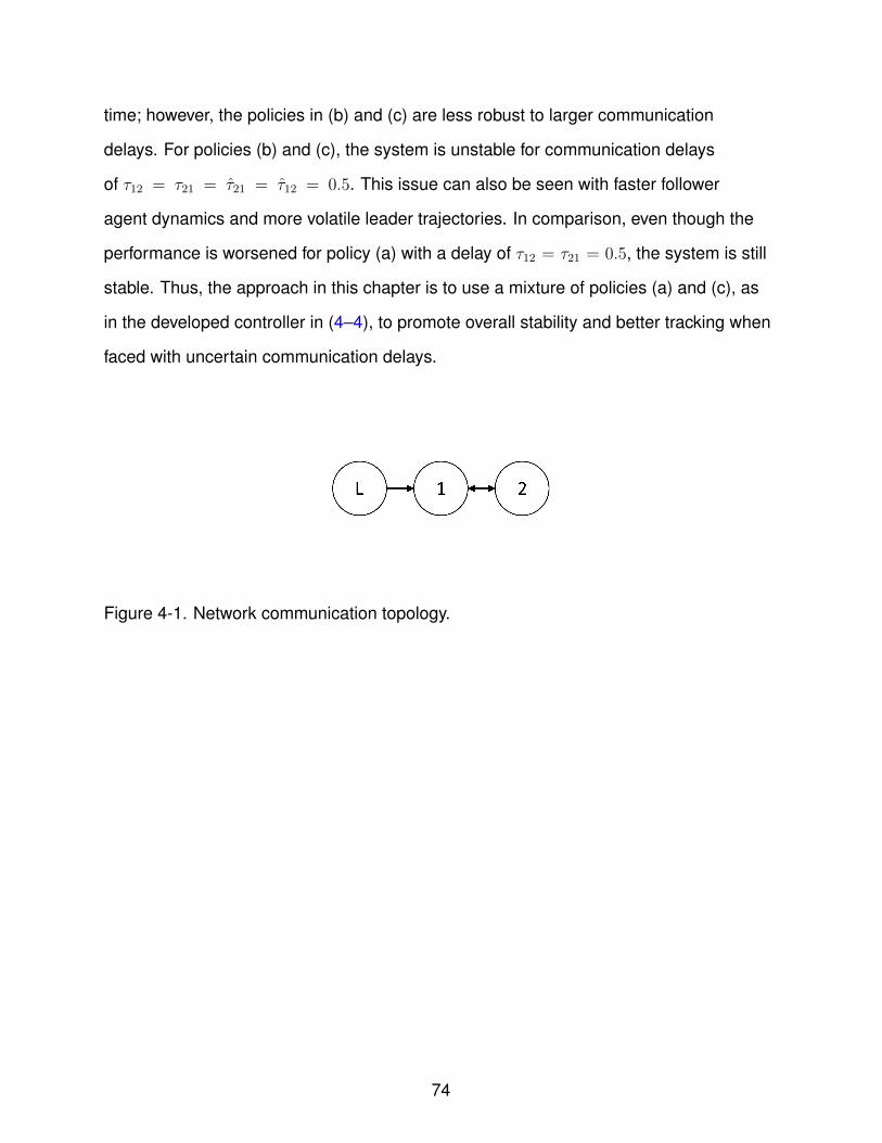
time; however, the policies in (b) and (c) are less robust to larger communication
delays. For policies (b) and (c), the system is unstable for communication delays
of τ12 = τ21 = τ21 = τ12 = 0.5. This issue can also be seen with faster follower
agent dynamics and more volatile leader trajectories. In comparison, even though the
performance is worsened for policy (a) with a delay of τ12 = τ21 = 0.5, the system is still
stable. Thus, the approach in this chapter is to use a mixture of policies (a) and (c), as
in the developed controller in (4–4), to promote overall stability and better tracking when
faced with uncertain communication delays.
Figure 4-1. Network communication topology.
74
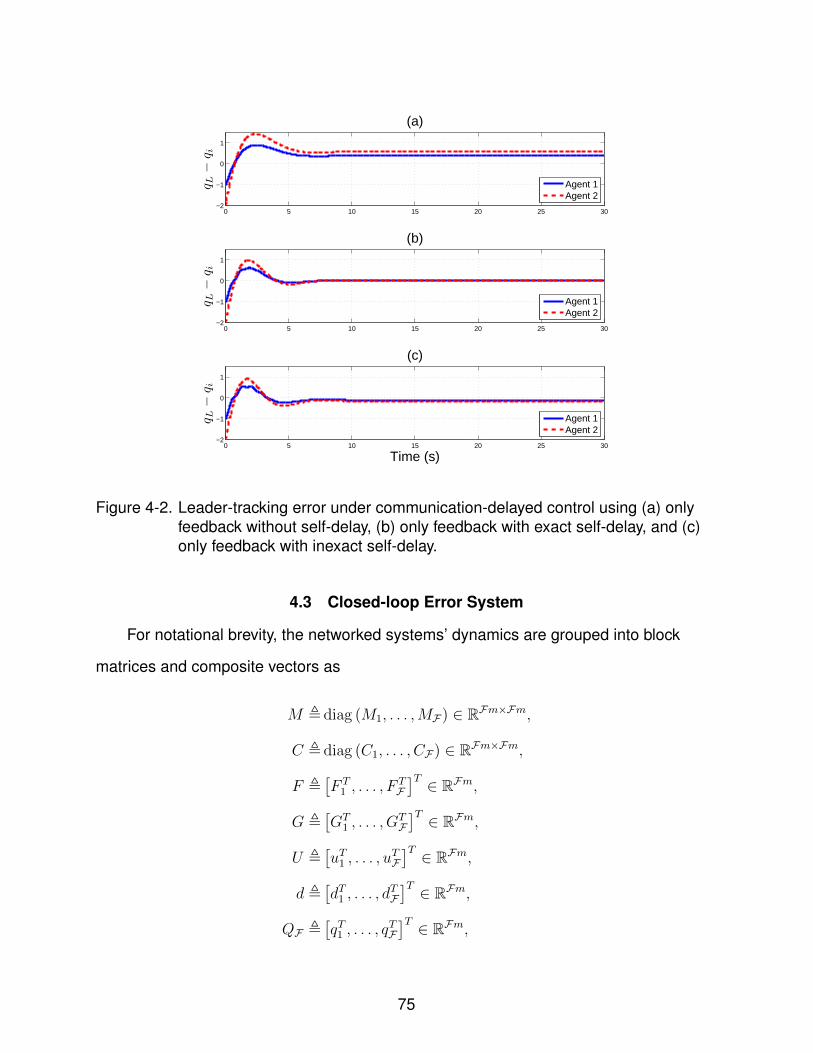
0 5 10 15 20 25 30−2
−1
0
1
q L−
q i
(a)
Agent 1Agent 2
0 5 10 15 20 25 30−2
−1
0
1
q L−
q i
(b)
Agent 1Agent 2
0 5 10 15 20 25 30−2
−1
0
1
Time (s)
q L−
q i
(c)
Agent 1Agent 2
Figure 4-2. Leader-tracking error under communication-delayed control using (a) onlyfeedback without self-delay, (b) only feedback with exact self-delay, and (c)only feedback with inexact self-delay.
4.3 Closed-loop Error System
For notational brevity, the networked systems’ dynamics are grouped into block
matrices and composite vectors as
M , diag (M1, . . . ,MF) ∈ RFm×Fm,
C , diag (C1, . . . , CF) ∈ RFm×Fm,
F ,[F T
1 , . . . , FTF]T ∈ RFm,
G ,[GT
1 , . . . , GTF]T ∈ RFm,
U ,[uT1 , . . . , u
TF]T ∈ RFm,
d ,[dT1 , . . . , d
TF]T ∈ RFm,
QF ,[qT1 , . . . , q
TF]T ∈ RFm,
75
such that
M (QF) QF + C(QF , QF
)QF + F
(QF
)+G (QF) = U + d (t) . (4–5)
Non-implemented error signals E , QL − QF ∈ RFm and R , E + λE ∈ RFm are
introduced to develop a network-wide closed-loop error system, where QL , 1F ⊗ qL.
Clearly, if ‖E‖ → 0, then the control objective is achieved.
To facilitate the description of the normalized neighbor feedback, let the matrix
A ∈ RF×F be defined as A , [aij], where aij , aij|NFi|
. Additionally, let the matrix
D ∈ RF×F be defined as D , diag {d1, . . . , dF}, where di ,∑
j∈NFi aij. For convenience
in describing the effects of the heterogeneous communication delays individually in
the closed-loop system, let the constant matrix Aij ∈ RFm×Fm be defined as Aij ,
(A ◦ 1ij) ⊗ Im, where ◦ denotes the Hadamard product and 1ij ∈ RF×F denotes
an indicator matrix, which has all zero entries except for the ith row and jth column,
which has a value of 1. Similarly, let the constant matrix Dij ∈ RFm×Fm be defined
as Dij , aij 1ii⊗Im. Note that∑
(j,i)∈EF Aij = A ⊗ Im and∑
(j,i)∈EF Dij = D ⊗ Im.
Also, let Bi ∈ RF×F be defined as Bi , B ◦ 1ii; note that∑
(L,i)∈EL Bi = B. Finally,
let the vectors Qτji , Qτji , QLτLi : R → RFm be defined as Qτji (t) , QF (t− τji (t)),
Qτji (t) , QF (t− τji (t)), QLτLi (t) , QL (t− τLi (t)).
By taking the time-derivative of R and premultiplying by the block inertia matrix M ,
the closed-loop error system is represented using (4–4) and (4–5) as
MR = CQF + F +G− d+MQL + λME − kRτ , (4–6)
76

where
Rτ ,[rTτ1, . . . , r
Tτm
]T= (κ1 + κ2)
∑(j,i)∈EF
Aij(Qτji + λQτji
)− κ1 (D ⊗ Im)
(QF + λQF
)− κ2
∑(j,i)∈EF
Dij(Qτji + λQτji
)+ (κ1 + κ2)
∑(L,i)∈EL
(Bi ⊗ Im)(QLτLi + λQLτLi
)− κ1 (B ⊗ Im)
(QF + λQF
)− κ2
∑(L,i)∈EL
(Bi ⊗ Im)(QτLi + λQτLi
).
After using the Fundamental Theorem of Calculus, the fact that(QL + λQL
)∈
Null (LF ⊗ Im) due to the structure of the Laplacian matrix, and adding and subtracting
the terms
k∑
(j,i)∈EF
(κ1Aij − κ2Lij)ˆ t
t−τji
(QL (s) + λQL (s)
)ds,
kκ2
∑(j,i)∈EF
Dijˆ t−τji
t−τji
(QL (s) + λQL (s)
)ds,
kκ2
∑(L,i)∈EL
(Bi ⊗ Im)
ˆ t−τLi
t−τLi
(QL (s) + λQL (s)
)ds,
(4–6) may be re-expressed as
77
MR =CQF + F +G− d+MQL + λME − kLBR
+ k∑
(j,i)∈EF
[(κ1Aij − κ2Lij)
ˆ t
t−τjiR (σ) dσ − κ2Dij
ˆ t−τji
t−τjiR (σ) dσ
]
− k∑
(j,i)∈EF
(κ1Aij − κ2Lij)ˆ t
t−τji
(QL (σ) + λQL (σ)
)dσ
+ kκ2
∑(j,i)∈EF
Dijˆ t−τji
t−τji
(QL (σ) + λQL (σ)
)dσ
− kκ2
∑(L,i)∈EL
(Bi ⊗ Im)
ˆ t
t−τLiR (σ) dσ
− kκ1
∑(L,i)∈EL
(Bi ⊗ Im)
ˆ t
t−τLi
(QL (σ) + λQL (σ)
)dσ
+ kκ2
∑(L,i)∈EL
(Bi ⊗ Im)
ˆ t−τLi
t−τLi
(QL (σ) + λQL (σ)
)dσ, (4–7)
where Lij , Dij − Aij ∈ RFm×Fm, and LB , (B + D −A ) ⊗ Im ∈ RFm×Fm,
which is symmetric and positive definite by Assumption 4.5 and [55]. The terms
CQF , F,G, d,MQL, λME in (4–7) can be compensated using traditional robust con-
trol methods; however, compensating for the terms which contain´ tt−τji R (σ) dσ,
´ t−τjit−τji R (σ) dσ, and
´ tt−τLi
R (σ) dσ is difficult due to the delayed state feedback and
amplification by the gain k. The following sections demonstrate that the decentralized
controller in (4–4) yields convergence to a neighborhood around the leader state for
each follower agent despite these delay-contributing terms for small enough time-
varying heterogeneous network delays and accurate enough delay estimates.
4.4 Convergence Analysis
Some constants, functions, and sets are introduced to facilitate the convergence
analysis. Let c, φ ∈ R>0 denote tunable constant parameters and let the constant c ∈ R
be defined as c , c(λ− 1
2
). Let the auxiliary constants k, η, θ ∈ R be defined as
k , k
(λ (LB)− (τ+¯τ)k3
2φ− ι1k
)− c
2, η , min
{c2, k
6
}, and θ , 1
2min
{2η, 1
τ+¯τ, ω, ω
τ, ω, ω¯τ
},
78
where the unknown constants ω, ω ∈ R are defined as ω , 1 − supt∈R,(j,i)∈EF τji and
ω , 1 − supt∈R,(j,i)∈EF∪EL˙τji, which are positive by Assumptions 4.6 and 4.7, and the
auxiliary constant ι1 ∈ R≥0 is defined as
ι1 ,(
¯QL + λ ¯QL
)τ ∑(j,i)∈EF
‖κ1Aij − κ2Lij‖+ κ2¯τ∑
(j,i)∈EF
‖Dij‖+ (κ1τ + κ2¯τ)
∑(L,i)∈EL
‖Bi‖
,
where the constant upper bounds ¯QL,¯QL ∈ R≥0 are defined such that supt∈R
∥∥∥QL (t)∥∥∥ ≤
¯QL and supt∈R
∥∥∥QL (t)∥∥∥ ≤ ¯QL.
The convergence analysis is constructed with the state y ∈ R2Fm+6 defined as
the composite vector2 y ,[ZT ,Ψ
121a,Ψ
121b,Ψ
122a,Ψ
122b,Ψ
123a,Ψ
123b
]T, where Z ∈ R2Fm is the
composite error vector Z ,
[ET RT
]T, and Ψ1a,Ψ1b,Ψ2a,Ψ2b,Ψ3a,Ψ3b denote LK
functionals defined as
Ψ1a ,φι2 |EF |k2
ˆ t
t−τ
ˆ t
s
∥∥∥R (σ)∥∥∥2
dσds, (4–8)
Ψ1b ,φ (ι3 |EF |+ ι4 |EL|)
k2
ˆ t
t−τ−¯τ
ˆ t
s
∥∥∥R (σ)∥∥∥2
dσds, (4–9)
Ψ2a ,2φ |EF | (τ ι2 |EF |+ (τ + ¯τ) (ι3 |EF |+ ι4 |EL|))
ωm2
·∑
(j,i)∈EF
ˆ t
t−τji
(‖(κ1Aij − κ2Lij)R (σ)‖2 + κ2
2 ‖DijR (σ)‖2)dσ, (4–10)
Ψ2b ,2φκ2
2 |EF | (τ ι2 |EF |+ (τ + ¯τ) (ι3 |EF |+ ι4 |EL|))ωm2
·ˆ t
t−τji
|EF | ∑(j,i)∈EF
‖DijR (σ)‖2 + |EL|∑
(L,i)∈EL
‖(Bi ⊗ Im)R (σ)‖2
dσ, (4–11)
2 The LK functionals are interpreted as time-varying signals and are incorporated intothe overall system state to facilitate the convergence analysis.
79

Ψ3a ,2φ |EF | (τ ι2 |EF |+ (τ + ¯τ) (ι3 |EF |+ ι4 |EL|))
ωm2
∑(j,i)∈EF
ˆ t
t−τji
ˆ t
s
(‖(κ1Aij − κ2Lij)R (σ)‖2
+ κ22 ‖DijR (σ)‖2
)dσds, (4–12)
Ψ3b ,2φκ2
2 |EF | (τ ι2 |EF |+ (τ + ¯τ) (ι3 |EF |+ ι4 |EL|))ωm2
·ˆ t
t−τji
ˆ t
s
|EF | ∑(j,i)∈EF
‖DijR (σ)‖2 + |EL|∑
(L,i)∈EL
‖(Bi ⊗ Im)R (σ)‖2
dσds, (4–13)
where the constants ι2, ι3, ι4 ∈ R>0 are defined as
ι2 , λ
∑(j,i)∈EF
(κ1Aij − κ2Lij) (κ1Aij − κ2Lij)T ,
ι3 , κ22 λ
∑(j,i)∈EF
D2ij
, ι4 , κ22 λ
∑(L,i)∈EL
B2i
.
To facilitate the description of the stability result in the following convergence analysis,
the constant parameters Nd0, Nd1, Nd2 ∈ R≥0 are defined as
Nd0 , d+ m ¯QL + supt∈R
S0
(QL, QL
), (4–14)
Nd1 ,2
m‖LB‖
(d
km+
¯QL
k+ι1m
)+ sup
t∈RS1
(QL, QL
), (4–15)
Nd2 ,4d2
k2m2+
2d
m
(¯QL
k2+
ι1km
)+ 4
(¯QL
k+ι1m
)2
+ supt∈R
S2
(QL, QL
), (4–16)
and the functions N0, N1, N2 : Π6p=1RFm → R are defined as
N0 , S0
(QF , QF
)− S0
(QL, QL
)+ f0
(E,R,QF , QF
), (4–17)
N1 , S1
(QF , QF
)− S1
(QL, QL
)+ f1 (E,R) , (4–18)
N2 , S2
(QF , QF
)− S2
(QL, QL
)+ f2
(E,R,QF , QF
), (4–19)
80

where the auxiliary functions S0, S1, S2 : RFm × RFm → R, f0 : Π4p=1RFm → R,
f1 : RFm × RFm → R, f2 : Π4p=1RFm → R, are defined as
S0 ,∥∥∥CQF + F +G
∥∥∥, S1 ,2
km2‖LB‖S0,
S2 ,4
k2m2S2
0 +2
m
(d
k2m+
¯QL
k2+
ι1km
)S0,
f0 , λm ‖R− λE‖+1
2
∥∥∥MR∥∥∥ ,
f1 ,4
m2‖LB‖2 ‖R‖+
2λ
km‖LB‖ ‖R− λE‖+
2
m2
∥∥∥∥∥∥∑
(j,i)∈EF
(κ1Aij − κ2Lij)
∥∥∥∥∥∥2
‖R‖
+2κ2
2 |EL|m2
∑(L,i)∈EL
‖Bi‖2 ‖R‖
+2 |EF | (1 + τ)
ωm2
∑(j,i)∈EF
(‖κ1Aij − κ2Lij‖2 + κ2
2 ‖Dij‖2) ‖R‖+
2κ22 |EF |2
(1 + ¯τ
)ωm2
∑(j,i)∈EF
‖Dij‖2 ‖R‖+2κ2
2 |EF | |EL|(1 + ¯τ
)ωm2
∑(L,i)∈EL
‖Bi‖2 ‖R‖ ,
f2 ,2λ
k2mS0 ‖R− λE‖+ 2λ
(d
k2m+
¯QL
k2+
ι1km
)‖R− λE‖+
4λ2
k2‖R− λE‖2 .
The functions N0, N1, N2 contain terms which can be upper-bounded by a function of
the error signals E and R. By [58, Lemma 5], there exist strictly increasing, radially
unbounded functions ρ0, ρ1, ρ2 : R≥0 → R≥0 which upper-bound N0, N1, N2 as3
∣∣∣N0
∣∣∣ ≤ ρ0 (‖Z‖) ‖Z‖ ,∣∣∣N1
∣∣∣ ≤ ρ1 (‖Z‖) ‖Z‖ ,∣∣∣N2
∣∣∣ ≤ ρ2 (‖Z‖) ‖Z‖ , (4–20)
3 While the smallest upper-bounding functions of the dynamics in N0, N1, N2 may notbe known, the bounding functions ρ0, ρ1, ρ2 may feasibly be constructed; for example, afriction coefficient may be unknown, but a sufficient upper bound can easily be deter-mined.
81
where the bounds for∣∣∣N0
∣∣∣ and∣∣∣N2
∣∣∣ are facilitated by adding and subtracting the expres-
sion f0
(E,R,QL, QL
)in N0 and the expression f2
(E,R,QL, QL
)in N2.
The set D ⊂ R2Fm+6 is defined as
D ,
{ξ ∈ R2Fm+6 | ‖ξ‖ < inf
{ρ−1
([√η,∞
))}},
where ρ : R≥0 → R≥0 is a strictly increasing, radially unbounded function defined as
ρ (‖Z‖) ,(
3ρ20 (‖Z‖)2k
+3φ2ρ2
1 (‖Z‖)2k
(τ ι2 |EF |+ (τ + ¯τ) (ι3 |EF |+ ι4 |EL|))2
+ φ (τ ι2 |EF |+ (τ + ¯τ) (ι3 |EF |+ ι4 |EL|)) ρ22 (‖Z‖)
) 12
, (4–21)
where the inverse image ρ−1 (Θ) ⊂ R for a set Θ ⊂ R is defined as ρ−1 (Θ) ,
{ξ ∈ R | ρ (ξ) ∈ Θ}. The stabilizing set of initial conditions, SD, is defined as
SD ,
{ξ ∈ D | ‖ξ‖ <
√min
{c2, m
2, 1}
max{c2, m
2, 1} inf
{ρ−1
([√η,∞
))}}. (4–22)
The following assumption provides a sufficient condition for the subsequent conver-
gence analysis by describing how small the network communication delays and delay
estimate errors should be to ensure convergence for a given network configuration.
Assumption 4.8. For a given network graph G and leader trajectory qL, the communica-
tion delay upper bound τ > 0 and delay estimate error upper bound ¯τ > 0 are sufficiently
small such that there exists a selection for the gain k and tuning parameter φ such that
λ (LB)− (τ + ¯τ) k3
2φ− ι1k > 0, (4–23)
82

inf
{ρ−1
([√η,∞
))}>
√2 max
{c2, m
2, 1}
θmin{c2, m
2, 1}
·(
3(N2d0 + φ2N2
d1 (τ ι2 |EF |+ (τ + ¯τ) (ι3 |EF |+ ι4 |EL|))2)
2k
+ φ (τ ι2 |EF |+ (τ + ¯τ) (ι3 |EF |+ ι4 |EL|))(
1
4+Nd2
)+ι14
) 12
. (4–24)
Remark 4.1. Assumption 4.8 ensures that there exists a selection for c such that k > 0.
Accordingly, let the value for c be assigned such that
0 < c < 2k
(λ (LB)− (τ + ˜τ)
2φk3 − ι1k
).
Assumption 4.8 also ensures that there exist stabilizing initial conditions and that the
ultimate bound on the convergence of each agent toward the leader state is within the
considered domain D.
Remark 4.2. Due to the presence of k, τ , and ¯τ in (4–21), there exist sufficiently small
values for τ and ¯τ such that there exists a value for the gain k such that (4–23) is
satisfied and inf
{ρ−1
([√η,∞
))}> δ for any δ ∈ R>0, i.e., the set SD can contain any
initial condition for a small enough τ and ¯τ . The tuning parameter φ is included to more
easily see the effect of communication delay on system convergence: the inequality
in (4–23) may be satisfied for large delay and delay estimate error upper bounds by
increasing φ, but doing so may result in a smaller set of stabilizing initial conditions SDand cause the sufficient condition in (4–24) to be unsatisfied. Thus, if the leader has
a trajectory with low acceleration and the follower agents have less volatile dynamics
and small disturbances, the conditions in Assumption 4.8 can be more easily satisfied
for larger delay and delay estimate error upper bounds by increasing φ, as seen in the
effects of (4–15), (4–16), (4–18), and (4–19) on (4–22) and (4–24).
The following theorem describes the convergence provided by the controller in
(4–4) for the synchronization of a network of agents with uncertain nonlinear dynamics
83
given by (4–1) which are affected by heterogeneous uncertain time-varying delays and
input disturbances.
Theorem 4.1. The communication-delayed controller in (4–4) provides UUB syn-
chronization for a network of agents with dynamics given by (4–1) in the sense that
lim supt→∞ ‖qi (t)− qL (t)‖ < ε for some ε ∈ R>0 and every follower agent i ∈ VF for all
initial conditions y (0) ∈ SD, provided that Assumptions 4.1-4.8 are satisfied and the gain
λ satisfies
λ >1
2. (4–25)
Proof. Consider the candidate Lyapunov function VL : D× R→ R≥0 defined as
VL ,c
2ETE +
1
2RTMR + Ψ1a + Ψ1b + Ψ2a + Ψ2b + Ψ3a + Ψ3b, (4–26)
which satisfies the inequalities
min{ c
2,m
2, 1}‖y‖2 ≤ VL (y, t) ≤ max
{ c2,m
2, 1}‖y‖2
for all y ∈ R2Fm+6 and t ∈ R, where the block inertia matrix M is interpreted as
a function of time, and the LK functionals Ψ1a, Ψ1b, Ψ2a, Ψ2b, Ψ3a, Ψ3b are defined in
(4–8)-(4–13).
By using the Leibniz rule and the definitions of τ , ¯τ, ω, ω, the time derivatives of
LK functionals Ψ1a,Ψ1b and upper bounds of the time derivatives of LK functionals
Ψ2a,Ψ2b,Ψ3a,Ψ3b are determined as
Ψ1a =φι2 |EF |k2
(τ∥∥∥R∥∥∥2
−ˆ t
t−τ
∥∥∥R (σ)∥∥∥2
dσ
), (4–27)
Ψ1b =φ (ι3 |EF |+ ι4 |EL|)
k2
((τ + ¯τ)
∥∥∥R∥∥∥2
−ˆ t
t−τ−¯τ
∥∥∥R (σ)∥∥∥2
dσ
), (4–28)
84
Ψ2a ≤2φ |EF | (τ ι2 |EF |+ (τ + ¯τ) (ι3 |EF |+ ι4 |EL|))
m2
·∑
(j,i)∈EF
(1
ω
(‖(κ1Aij − κ2Lij)R‖2 + κ2
2 ‖DijR‖2)−(‖(κ1Aij − κ2Lij)R (t− τji)‖2 + κ2
2 ‖DijR (t− τji)‖2
)), (4–29)
Ψ2b ≤2φκ2
2 |EF | (τ ι2 |EF |+ (τ + ¯τ) (ι3 |EF |+ ι4 |EL|))m2
·(|EF |ω
∑(j,i)∈EF
‖DijR‖2 +|EL|ω
∑(L,i)∈EL
‖(Bi ⊗ Im)R‖2
− |EF |∑
(j,i)∈EF
‖DijR (t− τji)‖2 − |EL|∑
(L,i)∈EL
‖(Bi ⊗ Im)R (t− τji)‖2
), (4–30)
Ψ3a ≤2φ |EF | (τ ι2 |EF |+ (τ + ¯τ) (ι3 |EF |+ ι4 |EL|))
m2
·∑
(j,i)∈EF
(−ˆ t
t−τji
(‖(κ1Aij − κ2Lij)R (σ)‖2 + κ2
2 ‖DijR (σ)‖2) dσ+τ
ω
(‖(κ1Aij − κ2Lij)R‖2 + κ2
2 ‖DijR‖2)), (4–31)
Ψ3b ≤2φκ2
2 |EF | (τ ι2 |EF |+ (τ + ¯τ) (ι3 |EF |+ ι4 |EL|))m2
·(−ˆ t
t−τji
|EF | ∑(j,i)∈EF
‖DijR (σ)‖2 + |EL|∑
(L,i)∈EL
‖(Bi ⊗ Im)R (σ)‖2
dσ
+¯τ |EF |ω
∑(j,i)∈EF
‖DijR‖2 +¯τ |EL|ω
∑(L,i)∈EL
‖(Bi ⊗ Im)R‖2
)(4–32)
Based on (4–8)-(4–13), feedback of the LK functionals in the state y of the Lyapunov
function VL is facilitated by developing the inequalities
Ψ1a
τ≤ φι2 |EF |
k2
ˆ t
t−τ
∥∥∥R (σ)∥∥∥2
dσ, (4–33)
Ψ1b
(τ + ¯τ)≤ φ (ι3 |EF |+ ι4 |EL|)
k2
ˆ t
t−τ−¯τ
∥∥∥R (σ)∥∥∥2
dσ, (4–34)
85
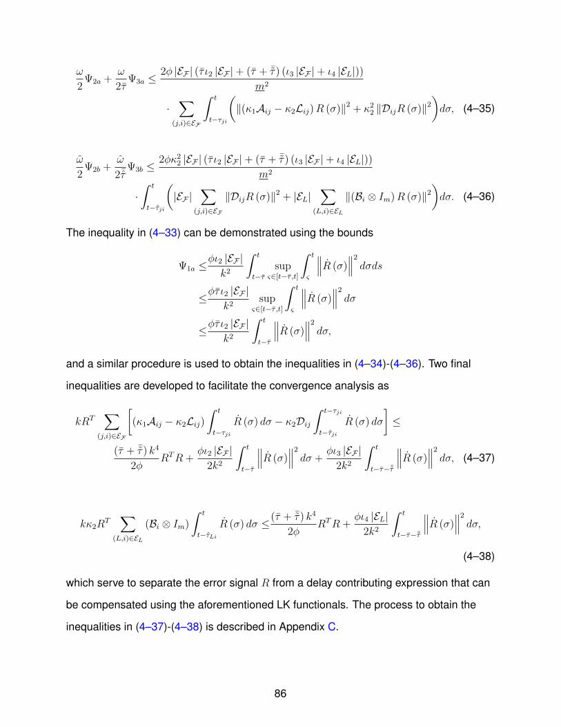
ω
2Ψ2a +
ω
2τΨ3a ≤
2φ |EF | (τ ι2 |EF |+ (τ + ¯τ) (ι3 |EF |+ ι4 |EL|))m2
·∑
(j,i)∈EF
ˆ t
t−τji
(‖(κ1Aij − κ2Lij)R (σ)‖2 + κ2
2 ‖DijR (σ)‖2
)dσ, (4–35)
ω
2Ψ2b +
ω
2¯τΨ3b ≤
2φκ22 |EF | (τ ι2 |EF |+ (τ + ¯τ) (ι3 |EF |+ ι4 |EL|))
m2
·ˆ t
t−τji
(|EF |
∑(j,i)∈EF
‖DijR (σ)‖2 + |EL|∑
(L,i)∈EL
‖(Bi ⊗ Im)R (σ)‖2
)dσ. (4–36)
The inequality in (4–33) can be demonstrated using the bounds
Ψ1a ≤φι2 |EF |k2
ˆ t
t−τsup
ς∈[t−τ ,t]
ˆ t
ς
∥∥∥R (σ)∥∥∥2
dσds
≤φτ ι2 |EF |k2
supς∈[t−τ ,t]
ˆ t
ς
∥∥∥R (σ)∥∥∥2
dσ
≤φτ ι2 |EF |k2
ˆ t
t−τ
∥∥∥R (σ)∥∥∥2
dσ,
and a similar procedure is used to obtain the inequalities in (4–34)-(4–36). Two final
inequalities are developed to facilitate the convergence analysis as
kRT∑
(j,i)∈EF
[(κ1Aij − κ2Lij)
ˆ t
t−τjiR (σ) dσ − κ2Dij
ˆ t−τji
t−τjiR (σ) dσ
]≤
(τ + ¯τ) k4
2φRTR +
φι2 |EF |2k2
ˆ t
t−τ
∥∥∥R (σ)∥∥∥2
dσ +φι3 |EF |
2k2
ˆ t
t−τ−¯τ
∥∥∥R (σ)∥∥∥2
dσ, (4–37)
kκ2RT∑
(L,i)∈EL
(Bi ⊗ Im)
ˆ t
t−τLiR (σ) dσ ≤(τ + ¯τ) k4
2φRTR +
φι4 |EL|2k2
ˆ t
t−τ−¯τ
∥∥∥R (σ)∥∥∥2
dσ,
(4–38)
which serve to separate the error signal R from a delay contributing expression that can
be compensated using the aforementioned LK functionals. The process to obtain the
inequalities in (4–37)-(4–38) is described in Appendix C.
86

By using the closed-loop error system in (4–7), the time derivative of (4–26) can be
expressed as
VL =cET (R− λE) +RT(CQF + F +G− d+MQL + λME − kLBR
)+
1
2RTMR
+ kRT∑
(j,i)∈EF
[(κ1Aij − κ2Lij)
ˆ t
t−τjiR (σ) dσ − κ2Dij
ˆ t−τji
t−τjiR (σ) dσ
]
− kRT∑
(j,i)∈EF
(κ1Aij − κ2Lij)ˆ t
t−τji
(QL (σ) + λQL (σ)
)dσ
+ kκ2RT∑
(j,i)∈EF
Dijˆ t−τji
t−τji
(QL (σ) + λQL (σ)
)dσ
− kκ2RT∑
(L,i)∈EL
(Bi ⊗ Im)
ˆ t
t−τLiR (σ) dσ
+ kRT
(−κ1
∑(L,i)∈EL
(Bi ⊗ Im)
ˆ t
t−τLi
(QL (σ) + λQL (σ)
)dσ
+ κ2
∑(L,i)∈EL
(Bi ⊗ Im)
ˆ t−τLi
t−τLi
(QL (σ) + λQL (σ)
)dσ
)+ Ψ1a + Ψ1b + Ψ2a + Ψ2b + Ψ3a + Ψ3b. (4–39)
After using the expressions in (4–27)-(4–32), the inequalities in (4–33)-(4–38), and
canceling terms, (4–39) can be upper-bounded as
87

VL =cET (R− λE) +1
2RTMR +
(τ + ¯τ) k4
φRTR
− Ψ1a
2τ− Ψ1b
2 (τ + ¯τ)− ω
2Ψ2a −
ω
2Ψ2b −
ω
2τΨ3a −
ω
2¯τΨ3b
+RT(CQF + F +G− d+MQL + λME − kLBR
)+ kι1 ‖R‖
+φτ ι2 |EF |+ φ (τ + ¯τ) (ι3 |EF |+ ι4 |EL|)
k2
∥∥∥R∥∥∥2
+2φ |EF | (τ ι2 |EF |+ (τ + ¯τ) (ι3 |EF |+ ι4 |EL|))
m2
((1 + τ)
ω
∑(j,i)∈EF
(‖(κ1Aij − κ2Lij)R‖2 + κ2
2 ‖DijR‖2)+κ2
2 |EF |(1 + ¯τ
)ω
∑(j,i)∈EF
‖DijR‖2 +κ2
2 |EL|(1 + ¯τ
)ω
∑(L,i)∈EL
‖(Bi ⊗ Im)R‖2
−∑
(j,i)∈EF
(‖(κ1Aij − κ2Lij)R (t− τji)‖2 + κ2
2 ‖DijR (t− τji)‖2
)
− κ22 |EF |
∑(j,i)∈EF
‖DijR (t− τji)‖2 − κ22 |EL|
∑(L,i)∈EL
‖(Bi ⊗ Im)R (t− τji)‖2
).
After expanding the term∥∥∥R∥∥∥2
using the closed-loop error system in (4–7), evaluat-
ing the resulting integrals, using Young’s inequality and the inequality ‖∑ni=1 ξ‖
2 ≤
n∑n
i=1 ‖ξ‖2 for ξ ∈ RFm, canceling terms, and using the bounding expressions in
(4–14)-(4–19), VL can be further upper-bounded as
VL ≤− c(λ− 1
2
)‖E‖2 − k
(λ (LB)− (τ + ¯τ) k3
φ− c
2k
)‖R‖2
− Ψ1a
2τ− Ψ1b
2 (τ + ¯τ)− ω
2Ψ2a −
ω
2Ψ2b −
ω
2τΨ3a −
ω
2¯τΨ3b
+(Nd0 + N0
)‖R‖+ φ (τ ι2 |EF |+ (τ + ¯τ) (ι3 |EF |+ ι4 |EL|))
·((Nd1 + N1
)‖R‖+Nd2 + N2
)+ kι1 ‖R‖ , (4–40)
88

where λ− 12
is positive by (4–25). After using the inequality kι1 ‖R‖ ≤ k2ι1 ‖R‖2 + ι14
, the
definitions for c and k, and the expressions in (4–20), (4–40) can be upper-bounded as
VL ≤− c ‖E‖2 − k ‖R‖2 − Ψ1a
2τ− Ψ1b
2 (τ + ¯τ)− ω
2Ψ2a −
ω
2Ψ2b −
ω
2τΨ3a −
ω
2¯τΨ3b
+(Nd0 + ρ0 (‖Z‖) ‖Z‖+ φ (τ ι2 |EF |+ (τ + ¯τ) (ι3 |EF |+ ι4 |EL|))
· (Nd1 + ρ1 (‖Z‖) ‖Z‖))‖R‖
+ φ (τ ι2 |EF |+ (τ + ¯τ) (ι3 |EF |+ ι4 |EL|)) (Nd2 + ρ2 (‖Z‖) ‖Z‖) +ι14. (4–41)
By using a fraction of the feedback −k ‖R‖2 to perform nonlinear damping on the other
terms multiplied by ‖R‖, and using the inequality ρ2 (‖Z‖) ‖Z‖ ≤ ρ22 (‖Z‖) ‖Z‖2 + 1
4,
(4–41) can be upper-bounded as
VL ≤− η ‖Z‖2 − Ψ1a
2τ− Ψ1b
2 (τ + ¯τ)− ω
2Ψ2a −
ω
2Ψ2b −
ω
2τΨ3a −
ω
2¯τΨ3b
−(η − 3ρ2
0 (‖Z‖)2k
− 3φ2ρ21 (‖Z‖)2k
(τ ι2 |EF |+ (τ + ¯τ) (ι3 |EF |+ ι4 |EL|))2
− φ (τ ι2 |EF |+ (τ + ¯τ) (ι3 |EF |+ ι4 |EL|)) ρ22 (‖Z‖)
)‖Z‖2
+3N2
d0
2k+
3φ2N2d1
2k(τ ι2 |EF |+ (τ + ¯τ) (ι3 |EF |+ ι4 |EL|))2
+ φ (τ ι2 |EF |+ (τ + ¯τ) (ι3 |EF |+ ι4 |EL|))(
1
4+Nd2
)+ι14. (4–42)
Provided Assumption 4.8 is satisfied, (4–42) can be upper-bounded as
VL ≤− θ ‖y‖2 +3N2
d0
2k+
3φ2N2d1
2k(τ ι2 |EF |+ (τ + ¯τ) (ι3 |EF |+ ι4 |EL|))2
+ φ (τ ι2 |EF |+ (τ + ¯τ) (ι3 |EF |+ ι4 |EL|))(
1
4+Nd2
)+ι14
for all y ∈ D, and thus,
VL ≤ −θ
2‖y‖2 ∀ ‖y‖ ≥
√2
θ
(3N2
d0
2k+
3φ2N2d1
2k(τ ι2 |EF |+ (τ + ¯τ) (ι3 |EF |+ ι4 |EL|))2
+ φ (τ ι2 |EF |+ (τ + ¯τ) (ι3 |EF |+ ι4 |EL|))(
1
4+Nd2
)+ι14
) 12
. (4–43)
89
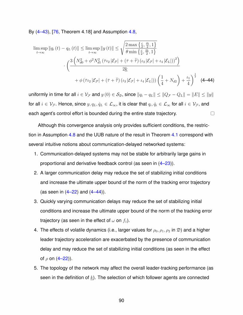
By (4–43), [76, Theorem 4.18] and Assumption 4.8,
lim supt→∞
‖qi (t)− qL (t)‖ ≤ lim supt→∞
‖y (t)‖ ≤√
2 max{c2, m
2, 1}
θmin{c2, m
2, 1}
·(3(N2d0 + φ2N2
d1 (τ ι2 |EF |+ (τ + ¯τ) (ι3 |EF |+ ι4 |EL|))2)
2k
+ φ (τ ι2 |EF |+ (τ + ¯τ) (ι3 |EF |+ ι4 |EL|))(
1
4+Nd2
)+ι14
) 12
(4–44)
uniformly in time for all i ∈ VF and y (0) ∈ SD, since ‖qi − qL‖ ≤ ‖QF −QL‖ = ‖E‖ ≤ ‖y‖
for all i ∈ VF . Hence, since y, qL, qL ∈ L∞, it is clear that qi, qi ∈ L∞ for all i ∈ VF , and
each agent’s control effort is bounded during the entire state trajectory.
Although this convergence analysis only provides sufficient conditions, the restric-
tion in Assumption 4.8 and the UUB nature of the result in Theorem 4.1 correspond with
several intuitive notions about communication-delayed networked systems:
1. Communication-delayed systems may not be stable for arbitrarily large gains in
proportional and derivative feedback control (as seen in (4–23)).
2. A larger communication delay may reduce the set of stabilizing initial conditions
and increase the ultimate upper bound of the norm of the tracking error trajectory
(as seen in (4–22) and (4–44)).
3. Quickly varying communication delays may reduce the set of stabilizing initial
conditions and increase the ultimate upper bound of the norm of the tracking error
trajectory (as seen in the effect of ω on f1).
4. The effects of volatile dynamics (i.e., larger values for ρ0, ρ1, ρ2 in D) and a higher
leader trajectory acceleration are exacerbated by the presence of communication
delay and may reduce the set of stabilizing initial conditions (as seen in the effect
of ρ on (4–22)).
5. The topology of the network may affect the overall leader-tracking performance (as
seen in the definition of k). The selection of which follower agents are connected
90
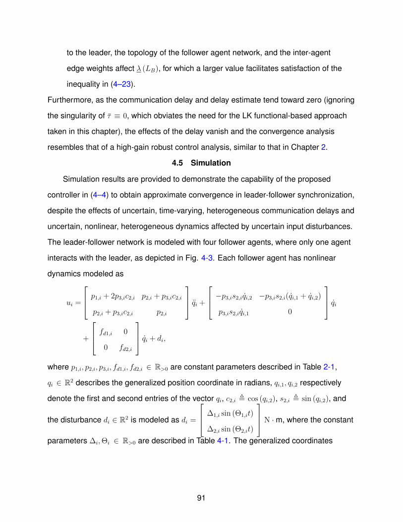
to the leader, the topology of the follower agent network, and the inter-agent
edge weights affect λ (LB), for which a larger value facilitates satisfaction of the
inequality in (4–23).
Furthermore, as the communication delay and delay estimate tend toward zero (ignoring
the singularity of τ ≡ 0, which obviates the need for the LK functional-based approach
taken in this chapter), the effects of the delay vanish and the convergence analysis
resembles that of a high-gain robust control analysis, similar to that in Chapter 2.
4.5 Simulation
Simulation results are provided to demonstrate the capability of the proposed
controller in (4–4) to obtain approximate convergence in leader-follower synchronization,
despite the effects of uncertain, time-varying, heterogeneous communication delays and
uncertain, nonlinear, heterogeneous dynamics affected by uncertain input disturbances.
The leader-follower network is modeled with four follower agents, where only one agent
interacts with the leader, as depicted in Fig. 4-3. Each follower agent has nonlinear
dynamics modeled as
ui =
p1,i + 2p3,ic2,i p2,i + p3,ic2,i
p2,i + p3,ic2,i p2,i
qi +
−p3,is2,iqi,2 −p3,is2,i(qi,1 + qi,2)
p3,is2,iqi,1 0
qi+
fd1,i 0
0 fd2,i
qi + di,
where p1,i, p2,i, p3,i, fd1,i, fd2,i ∈ R>0 are constant parameters described in Table 2-1,
qi ∈ R2 describes the generalized position coordinate in radians, qi,1, qi,2 respectively
denote the first and second entries of the vector qi, c2,i , cos (qi,2), s2,i , sin (qi,2), and
the disturbance di ∈ R2 is modeled as di =
∆1,i sin (Θ1,it)
∆2,i sin (Θ2,it)
N ·m, where the constant
parameters ∆i,Θi ∈ R>0 are described in Table 4-1. The generalized coordinates
91
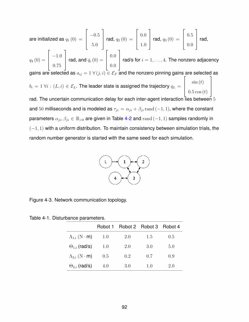
are initialized as q1 (0) =
−0.5
5.0
rad, q2 (0) =
0.0
1.0
rad, q3 (0) =
0.5
0.0
rad,
q4 (0) =
−1.0
0.75
rad, and qi (0) =
0.0
0.0
rad/s for i = 1, . . . , 4. The nonzero adjacency
gains are selected as aij = 1 ∀ (j, i) ∈ EF and the nonzero pinning gains are selected as
bi = 1 ∀i : (L, i) ∈ EL. The leader state is assigned the trajectory qL =
sin (t)
0.5 cos (t)
rad. The uncertain communication delay for each inter-agent interaction lies between 5
and 50 milliseconds and is modeled as τji = αji + βji rand (−1, 1), where the constant
parameters αji, βji ∈ R>0 are given in Table 4-2 and rand (−1, 1) samples randomly in
(−1, 1) with a uniform distribution. To maintain consistency between simulation trials, the
random number generator is started with the same seed for each simulation.
Figure 4-3. Network communication topology.
Table 4-1. Disturbance parameters.
Robot 1 Robot 2 Robot 3 Robot 4
Λ1,i (N ·m) 1.0 2.0 1.5 0.5
Θ1,i (rad/s) 1.0 2.0 3.0 5.0
Λ2,i (N ·m) 0.5 0.2 0.7 0.9
Θ2,i (rad/s) 4.0 3.0 1.0 2.0
92
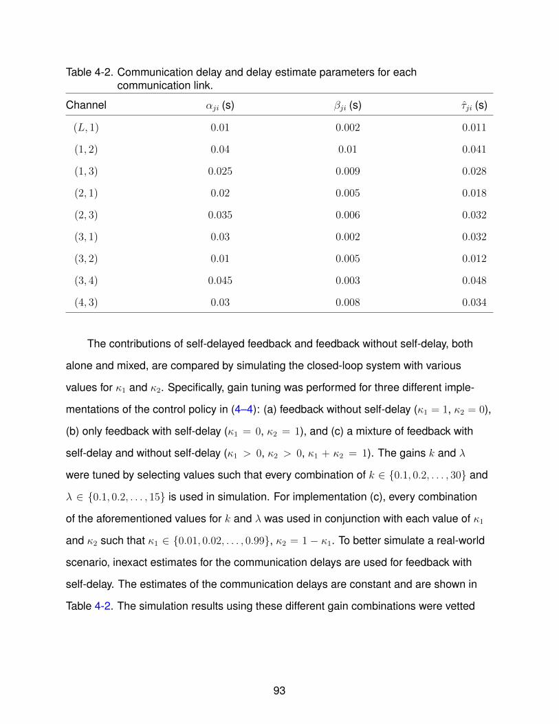
Table 4-2. Communication delay and delay estimate parameters for eachcommunication link.
Channel αji (s) βji (s) τji (s)
(L, 1) 0.01 0.002 0.011
(1, 2) 0.04 0.01 0.041
(1, 3) 0.025 0.009 0.028
(2, 1) 0.02 0.005 0.018
(2, 3) 0.035 0.006 0.032
(3, 1) 0.03 0.002 0.032
(3, 2) 0.01 0.005 0.012
(3, 4) 0.045 0.003 0.048
(4, 3) 0.03 0.008 0.034
The contributions of self-delayed feedback and feedback without self-delay, both
alone and mixed, are compared by simulating the closed-loop system with various
values for κ1 and κ2. Specifically, gain tuning was performed for three different imple-
mentations of the control policy in (4–4): (a) feedback without self-delay (κ1 = 1, κ2 = 0),
(b) only feedback with self-delay (κ1 = 0, κ2 = 1), and (c) a mixture of feedback with
self-delay and without self-delay (κ1 > 0, κ2 > 0, κ1 + κ2 = 1). The gains k and λ
were tuned by selecting values such that every combination of k ∈ {0.1, 0.2, . . . , 30} and
λ ∈ {0.1, 0.2, . . . , 15} is used in simulation. For implementation (c), every combination
of the aforementioned values for k and λ was used in conjunction with each value of κ1
and κ2 such that κ1 ∈ {0.01, 0.02, . . . , 0.99}, κ2 = 1 − κ1. To better simulate a real-world
scenario, inexact estimates for the communication delays are used for feedback with
self-delay. The estimates of the communication delays are constant and are shown in
Table 4-2. The simulation results using these different gain combinations were vetted
93

using the leader tracking-based cost function
J ,4∑i=1
2∑j=1
rms (qL,j − qi,j) ,
where rms (·) denotes the RMS of the argument’s sampled trajectory between 0 and
20 seconds, qL,j denotes the jth entry of the vector qL, and qi,j denotes the jth entry
of the vector qi. The gain combinations which produced the lowest cost for the three
different control implementations and the associated costs are shown in Table 4-3, and
the according simulation results are shown in Fig. 4-4 - 4-6.
As seen in Table 4-3, for the given simulation setting, control implementation (c)
(mixture of feedback without self-delay and feedback with self-delay) gives a 12.5%
performance increase over implementation (a) (no self-delayed feedback) and a 58.8%
performance increase over implementation (b) (only self-delayed feedback). Whereas
implementation (a) remains stable for a selection of the gain k up to 30, implementation
(b) produces an unstable closed-loop system if k ≥ 3.6 and λ = 15, which demonstrates
the sensitivity of only using feedback with self-delay. Implementation (c) produces the
best leader-tracking performance by combining feedback without self-delay, which is
helpful in stabilization, and feedback with self-delay, which can provide better tracking
performance by comparing signals closer in time.
Table 4-3. Tuned gains and associated costs for (a) feedback without self-delay, (b) onlyfeedback with self-delay, and (c) a mixture of feedback with self-delay andwithout self-delay.
k λ κ1 κ2 J
(a) 30 15 1 0 52.2
(b) 3.5 15 0 1 111
(c) 30 15 0.71 0.29 45.7
94
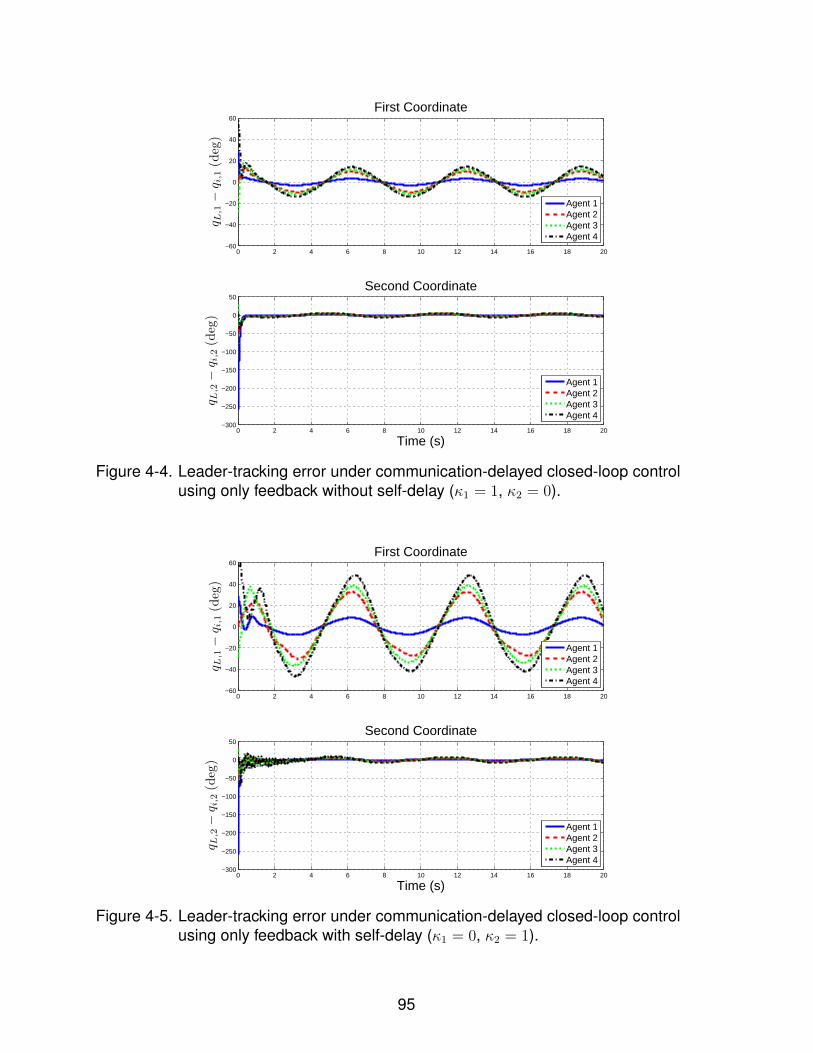
0 2 4 6 8 10 12 14 16 18 20−60
−40
−20
0
20
40
60
q L,1−
q i,1(deg)
First Coordinate
Agent 1Agent 2Agent 3Agent 4
0 2 4 6 8 10 12 14 16 18 20−300
−250
−200
−150
−100
−50
0
50
Time (s)
q L,2−
q i,2(deg)
Second Coordinate
Agent 1Agent 2Agent 3Agent 4
Figure 4-4. Leader-tracking error under communication-delayed closed-loop controlusing only feedback without self-delay (κ1 = 1, κ2 = 0).
0 2 4 6 8 10 12 14 16 18 20−60
−40
−20
0
20
40
60
q L,1−
q i,1(deg)
First Coordinate
Agent 1Agent 2Agent 3Agent 4
0 2 4 6 8 10 12 14 16 18 20−300
−250
−200
−150
−100
−50
0
50
Time (s)
q L,2−
q i,2(deg)
Second Coordinate
Agent 1Agent 2Agent 3Agent 4
Figure 4-5. Leader-tracking error under communication-delayed closed-loop controlusing only feedback with self-delay (κ1 = 0, κ2 = 1).
95
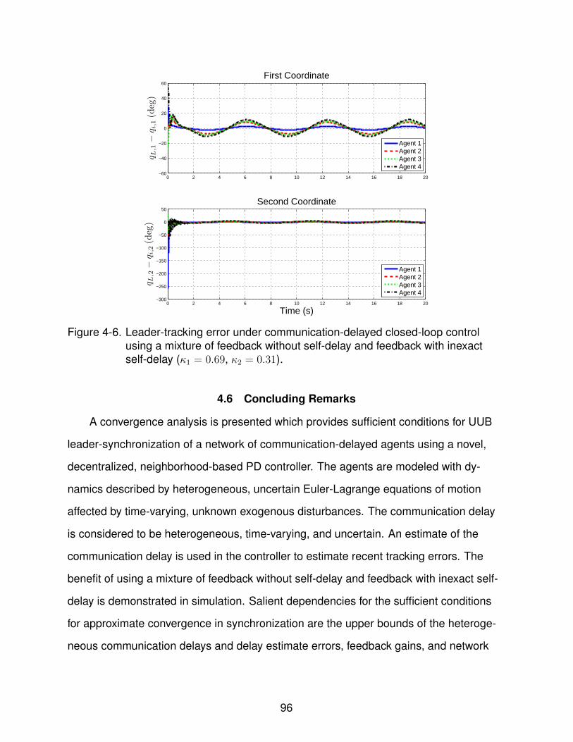
0 2 4 6 8 10 12 14 16 18 20−60
−40
−20
0
20
40
60
q L,1−
q i,1(deg)
First Coordinate
Agent 1Agent 2Agent 3Agent 4
0 2 4 6 8 10 12 14 16 18 20−300
−250
−200
−150
−100
−50
0
50
Time (s)
q L,2−
q i,2(deg)
Second Coordinate
Agent 1Agent 2Agent 3Agent 4
Figure 4-6. Leader-tracking error under communication-delayed closed-loop controlusing a mixture of feedback without self-delay and feedback with inexactself-delay (κ1 = 0.69, κ2 = 0.31).
4.6 Concluding Remarks
A convergence analysis is presented which provides sufficient conditions for UUB
leader-synchronization of a network of communication-delayed agents using a novel,
decentralized, neighborhood-based PD controller. The agents are modeled with dy-
namics described by heterogeneous, uncertain Euler-Lagrange equations of motion
affected by time-varying, unknown exogenous disturbances. The communication delay
is considered to be heterogeneous, time-varying, and uncertain. An estimate of the
communication delay is used in the controller to estimate recent tracking errors. The
benefit of using a mixture of feedback without self-delay and feedback with inexact self-
delay is demonstrated in simulation. Salient dependencies for the sufficient conditions
for approximate convergence in synchronization are the upper bounds of the heteroge-
neous communication delays and delay estimate errors, feedback gains, and network
96
connectivity. Some prominent assumptions are that the follower communication network
is undirected and at least one follower agent receives information from the leader.
The approach in this chapter provides a framework for exploring other methods to
improve the performance of decentralized control in networks affected by communica-
tion delay. For example, the controller in (4–4) may be improved by the development of
a decentralized algorithm which changes edge weights or the neighbor set based on
local network structure and estimates of neighbors’ communication delays; customiza-
tion of κ1 and κ2 for each neighbor based on the delay estimates; and decentralized
communication-based algorithms which allow each agent to predict the leader trajectory,
similar to that in [43], thereby reducing the impact of the propagation of communication
delays through agents’ dynamics.
97
CHAPTER 5DECENTRALIZED SYNCHRONIZATION OF UNCERTAIN NONLINEAR SYSTEMS
WITH A REPUTATION ALGORITHM
This chapter considers a decentralized network control scenario in which agents
use both communication and sensing to interact. The communication is assumed to
be continuously available, but have possible inaccuracies due to poor self localization.
The neighbor sensor measurements are assumed to provide accurate relative position
information, but only occur intermittently. Because the sensor measurements are
modeled as intermittent, and therefore may not be frequent enough to be implemented
in closed-loop control, they are used to vet communicated information so that an agent
can rely more on information from more reliable neighbors. A reputation algorithm
is developed in which each agent quantitatively evaluates the trust of each neighbor
based on the discrepancy between communicated and sensed information. The
trust values are then used in the reputation algorithm so that agents communicate
about a mutually shared neighbor to collaboratively obtain a reputation. Each agent’s
contribution to the reputation algorithm is weighted by that neighbor’s own reputation.
The result of the reputation algorithm is used to update consensus weights which
affect the relative weighting in the decentralized control policy’s use of a neighbor’s
communicated information compared to other neighbors’, if an agent has multiple
neighbors. However, the consensus weight updates alter the feedback structure of and
introduce discontinuities into the network-wide closed-loop system. Concepts from
switching theory and the sensitivity of the solution to the Lyapunov Equation are used to
address the effects of asymmetric consensus weight updates and develop a dwell-time
that must elapse between successive updates in the network.
5.1 Problem Formulation
5.1.1 Network Properties
Similar to the previous chapters, the follower graph is modeled such that the
network topology is static, i.e., VF and EF do not vary in time. However, dissimilar
98
to the previous chapters, the edge weights are modeled as time-varying such that
aij : R → R>0 if (j, i) ∈ EF and aij = 0 otherwise for every follower-to-follower edge
(j, i) ∈ EF . Furthermore, this chapter considers the more general directed graph to
describe the network topology, i.e., interaction links may not necessarily be bidirectional.
The following assumption specifies the class of networks considered in the following
analysis, where the term “strongly-connected” indicates that there exists a sequence of
directed edges between any two nodes.
Assumption 5.1. The graph GF is strongly-connected and at least one agent is con-
nected to the leader.
5.1.2 Dynamic Models and Properties
Let the dynamics of each follower agent i ∈ VF be modeled with uncertain second-
order nonlinear dynamics as
xi = fi (xi, xi) + ui, (5–1)
where xi ∈ Rm is the state, fi : Rm × Rm → Rm denotes the uncertain nonlinear drift
dynamics, and ui ∈ Rm is the control input to be designed. The time-varying trajectory
of the leader state is denoted by xL : R → Rm, which is known by at least one of the
follower agents. The following assumptions concerning the follower agents’ dynamics
and the leader trajectory are made to simplify the analysis.
Assumption 5.2. The drift dynamics, fi, are first-order differentiable, i.e., the first-order
derivative exists and is bounded if xi, xi, xi are bounded, for every follower agent i ∈ VF .
Assumption 5.3. The leader state trajectory is sufficiently smooth such that xL, xL, xL
are bounded.
Note that the dynamics in (5–1) can be represented in Euler-Lagrange form if the
inertia matrix is known and used in the controller. The inertia matrix is omitted from the
dynamics to simplify the subsequent analysis.
99
5.1.3 Neighbor Communication and Sensing
Neighboring follower agents use both communication and sensing to interact with
each other. Communication of continuous estimates of the state information (xj, xj) of
agent j ∈ VF is available to its neighbor i ∈ NFj at all times; however, the communicated
information may be inaccurate due to imperfect knowledge of the agent’s own state
in the global coordinate system. For example, a UAV in a network may transmit an
inaccurate estimate of its own position. However, intermittent neighbor sensing of an
agent j ∈ VF by a neighbor i ∈ NFj provides accurate relative position information
(xj − xi) at isolated points in time. For example, an agent may be able to observe
neighbors using a camera, but may only determine the relative position intermittently
due to occlusions, low hardware refresh rates, etc. As a consequence, neighbor sensing
may not be frequent enough for stability in a control algorithm which uses neighbor
sensing alone. Thus, each agent must use both continuous, possibly inaccurate
neighbor communication and accurate, intermittent neighbor sensing to accomplish
a control objective. Because the intermittent neighbor sensing is accurate, it may be
used to vet and intelligently use the communicated state information. Let xi, ˙xi denote
the estimates of xi, xi computed by agent i ∈ VF . The following assumptions concerning
the communicated state information are made to facilitate the following analysis.
Assumption 5.4. The difference between the estimated state information xi, ˙xi and the
actual state information xi, xi is bounded for each follower agent i ∈ VF , i.e., there exist
known positive constants x, ¯x ∈ R such that ‖xi − xi‖ ≤ x and∥∥∥ ˙xi − xi
∥∥∥ ≤ ¯x for each
i ∈ VF and all time.
Assumption 5.5. Information communicated from the leader agent is accurate.
As seen in the following section, Assumption 5.5 is critical to achieving close
synchronization with the leader. Whereas it may be difficult to guarantee perfect
state communication for each agent, it is plausible to guarantee Assumption 5.5 by
100
outfitting only the leader agent with more robust localization equipment or monitoring by
personnel.
5.1.4 Control Objective
Similar to traditional synchronization approaches (cf. [3, 7, 8, 77]), the objective is to
drive the states of the networked agents towards the state of the network leader such
that lim supt→∞ ‖xi (t)− xL (t)‖ ≤ ε with a small ε through advantageous use of the
communicated and sensed information.
5.2 Controller Development
5.2.1 Error System
The error signal in decentralized control traditionally has the form∑
j∈NFi aij (xj − xi)+
bi (xL − xi). However, since accurate state information is not always available to each
agent, a decentralized neighbor-based error signal is developed based on communi-
cated information as
ei ,∑j∈NFi
aij (xj − xi) + bi (xL − xi) . (5–2)
In (5–2), the first term provides communication-based feedback for comparison to
neighboring follower agents and the second term provides communication-based
feedback for comparison to the leader agent, if that connection exists. Hence, instead of
imposing discontinuities on the error signal by using the accurate sensed relative state
whenever a sensor measurement is available, the strategy is to use the communicated
information for feedback and update the edge weights aij based on the discrepancy
between the communicated and sensed information, as demonstrated in Section 5.2.3.
These edge weights will be updated so that neighbors which seem to provide more
accurate information have a greater impact on the synchronization performance.
An auxiliary error signal is analogously defined as
ri ,∑j∈NFi
aij
(˙xj − ˙xi
)+ bi
(xL − ˙xi
)+ λei, (5–3)
where λ ∈ R is a positive constant tuning parameter.
101
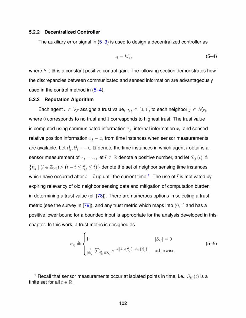
5.2.2 Decentralized Controller
The auxiliary error signal in (5–3) is used to design a decentralized controller as
ui = kri, (5–4)
where k ∈ R is a constant positive control gain. The following section demonstrates how
the discrepancies between communicated and sensed information are advantageously
used in the control method in (5–4).
5.2.3 Reputation Algorithm
Each agent i ∈ VF assigns a trust value, σij ∈ [0, 1], to each neighbor j ∈ NFi,
where 0 corresponds to no trust and 1 corresponds to highest trust. The trust value
is computed using communicated information xj, internal information xi, and sensed
relative position information xj − xi from time instances when sensor measurements
are available. Let t1ij, t2ij, . . . ∈ R denote the time instances in which agent i obtains a
sensor measurement of xj − xi, let t ∈ R denote a positive number, and let Sij (t) ,{tlij | (l ∈ Z>0) ∧
(t− t ≤ tlij ≤ t
)}denote the set of neighbor sensing time instances
which have occurred after t − t up until the current time.1 The use of t is motivated by
expiring relevancy of old neighbor sensing data and mitigation of computation burden
in determining a trust value (cf. [78]). There are numerous options in selecting a trust
metric (see the survey in [79]), and any trust metric which maps into (0, 1] and has a
positive lower bound for a bounded input is appropriate for the analysis developed in this
chapter. In this work, a trust metric is designed as
σij ,
1 |Sij| = 0
1|Sij |
∑tlij∈Sij
e−s‖xij(tlij)−ˆxij(tlij)‖ otherwise,
(5–5)
1 Recall that sensor measurements occur at isolated points in time, i.e., Sij (t) is afinite set for all t ∈ R.
102

where s ∈ R is a positive tuning parameter, xij , xj − xi is the relative position
obtained via neighbor sensing, and ˆxij , xj − xi is the relative position obtained via
communication of the state estimate xj and the internal position estimate xi maintained
by agent i.2 In (5–5), a trust value of 1 is computed if there are no recent sensor
measurements (i.e., Sij (t) is an empty set). If there are recent sensor measurements,
the term e−s‖xij(tlij)−ˆxij(tlij)‖ maps the discrepancy between the estimated relative
position and the actual relative position to (0, 1]. The result is then averaged with the
corresponding values for the other sensor measurements to obtain the overall trust
value. Note that xij and ˆxij may differ due to an inaccurate estimate of xi, i.e., an agent’s
trust of a neighbor may be affected by an inaccurate estimate of its own state. However,
because xi is necessary to provide a continuous comparison to neighbors’ states,
there is no utility in determining a trust value for an agent’s own state. Future work
may investigate methods to better estimate an agent’s own state based on neighbor
feedback.
Each follower agent i ∈ VF maintains a reputation value ζij : Π2|NFi∩NFj|+2
l=1 R→ R for
every neighbor j ∈ NFi based on recommendations from mutual neighbors, where the
reputation is updated using trust values as
ζij =∑
n∈NFi∩NFj
ηζiζin (ζnj − ζij) + ησi (σij − ζij) (5–6)
with the initial condition ζij (0) = 1, where a higher reputation corresponds to higher
reliability and ηζi, ησi ∈ R>0 are tunable gains that weigh how much recommended
information is relied upon compared to directly observed information. Similar to [49],
the first term in (5–6) contributes towards the reputation update by agent i of agent j
based on the reputation of j held by mutual neighbors n ∈ NFi∩NFj via communication.
2 Similar to [78], the summation in (5–5) can be weighted by how much time haselapsed since the measurements took place, if relevant for the intended application.
103

Dissimilar to [49], the contribution of a mutual neighbor to the reputation update is
weighted by the reputation of that agent, as seen in the multiplication by ζin. Thus, an
agent which has a low reputation has less significant impact in recommendation of a
reputation value. The second term in (5–6) directly uses the observation-based trust
value to update reputation. As shown in Appendix D, for each connection (j, i) ∈ EF ,
the reputation value ζij is bounded such that ζij ∈ [σ∗, 1] for all t ∈ R, where σ∗ ∈ R is a
bounding constant such that σij ≥ σ∗ for all t ∈ R, and σ∗ > 0 by Assumption 5.4.
5.2.4 Edge Weight Updates
The reputation values, ζij, are used to update the edge weight values, aij, which
quantify how much influence a neighbor has in the decentralized control policy in
(5–4). However, changes to the edge weight values affect the feedback in (5–4), which
affects the response of the closed-loop system. To control the effects of the edge
weight updates on the systems’ feedback structure, and based on the subsequent
convergence analysis, the edge weights are updated at discrete times in predefined
time intervals. Thus, the adjacency matrix A and the Laplacian matrix LF are functions
of time, i.e., A : R → RF×F and LF : R → RF×F , where the adjacency matrix is
initialized such that aij (0) = 1|NFi|
if (j, i) ∈ EF , i.e., all follower-to-follower connections
are equally weighted at t = 0. However, if the edge weights are updated too rapidly,
then the resulting frequent discontinuities in the switched closed-loop system may cause
instability (cf. [80, Chapter 2]). Thus, a dwell-time (cf. [80, Chapter 3]), τd ∈ R>0, is
developed to describe the minimum amount of time that must elapse before an agent
i ∈ VF can update its edge weight values, {aij | j ∈ NFi}, since its last update (or the
initial time), and is computed before the control implementation. Implementation of the
dwell-time is decentralized in the sense that an agent may update its edge weights at
different times from other neighbors as long as the elapsed time between successive
updates is not shorter than the dwell-time. The network topology-dependent minimum
dwell-time is given in Section 5.5 and is based on the subsequent convergence analysis.
104
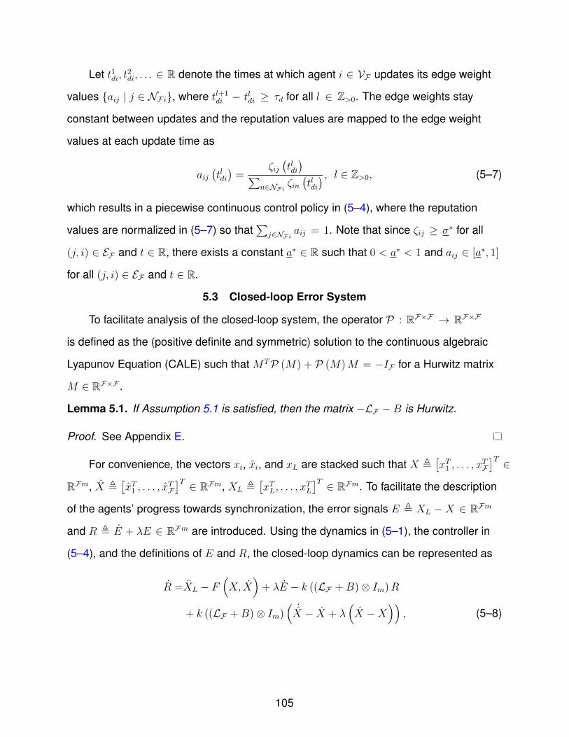
Let t1di, t2di, . . . ∈ R denote the times at which agent i ∈ VF updates its edge weight
values {aij | j ∈ NFi}, where tl+1di − tldi ≥ τd for all l ∈ Z>0. The edge weights stay
constant between updates and the reputation values are mapped to the edge weight
values at each update time as
aij(tldi)
=ζij(tldi)∑
n∈NFi ζin(tldi) , l ∈ Z>0, (5–7)
which results in a piecewise continuous control policy in (5–4), where the reputation
values are normalized in (5–7) so that∑
j∈NFi aij = 1. Note that since ζij ≥ σ∗ for all
(j, i) ∈ EF and t ∈ R, there exists a constant a∗ ∈ R such that 0 < a∗ < 1 and aij ∈ [a∗, 1]
for all (j, i) ∈ EF and t ∈ R.
5.3 Closed-loop Error System
To facilitate analysis of the closed-loop system, the operator P : RF×F → RF×F
is defined as the (positive definite and symmetric) solution to the continuous algebraic
Lyapunov Equation (CALE) such that MTP (M) + P (M)M = −IF for a Hurwitz matrix
M ∈ RF×F .
Lemma 5.1. If Assumption 5.1 is satisfied, then the matrix −LF −B is Hurwitz.
Proof. See Appendix E.
For convenience, the vectors xi, xi, and xL are stacked such that X ,[xT1 , . . . , x
TF]T ∈
RFm, X ,[xT1 , . . . , x
TF]T ∈ RFm, XL ,
[xTL, . . . , x
TL
]T ∈ RFm. To facilitate the description
of the agents’ progress towards synchronization, the error signals E , XL − X ∈ RFm
and R , E + λE ∈ RFm are introduced. Using the dynamics in (5–1), the controller in
(5–4), and the definitions of E and R, the closed-loop dynamics can be represented as
R =XL − F(X, X
)+ λE − k ((LF +B)⊗ Im)R
+ k ((LF +B)⊗ Im)(
˙X − X + λ
(X −X
)), (5–8)
105
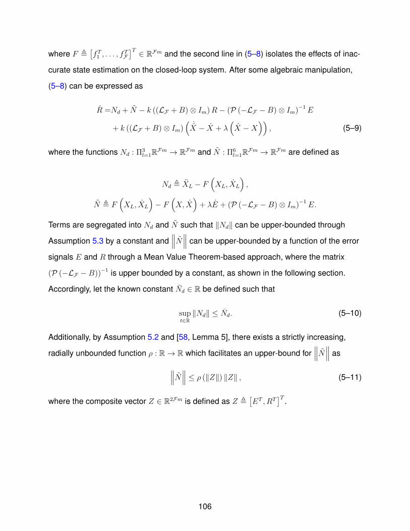
where F ,[fT1 , . . . , f
TF]T ∈ RFm and the second line in (5–8) isolates the effects of inac-
curate state estimation on the closed-loop system. After some algebraic manipulation,
(5–8) can be expressed as
R =Nd + N − k ((LF +B)⊗ Im)R− (P (−LF −B)⊗ Im)−1E
+ k ((LF +B)⊗ Im)(
˙X − X + λ
(X −X
)), (5–9)
where the functions Nd : Π3l=1RFm → RFm and N : Π6
l=1RFm → RFm are defined as
Nd , XL − F(XL, XL
),
N , F(XL, XL
)− F
(X, X
)+ λE + (P (−LF −B)⊗ Im)−1E.
Terms are segregated into Nd and N such that ‖Nd‖ can be upper-bounded through
Assumption 5.3 by a constant and∥∥∥N∥∥∥ can be upper-bounded by a function of the error
signals E and R through a Mean Value Theorem-based approach, where the matrix
(P (−LF −B))−1 is upper bounded by a constant, as shown in the following section.
Accordingly, let the known constant Nd ∈ R be defined such that
supt∈R‖Nd‖ ≤ Nd. (5–10)
Additionally, by Assumption 5.2 and [58, Lemma 5], there exists a strictly increasing,
radially unbounded function ρ : R→ R which facilitates an upper-bound for∥∥∥N∥∥∥ as∥∥∥N∥∥∥ ≤ ρ (‖Z‖) ‖Z‖ , (5–11)
where the composite vector Z ∈ R2Fm is defined as Z ,[ET , RT
]T .
106
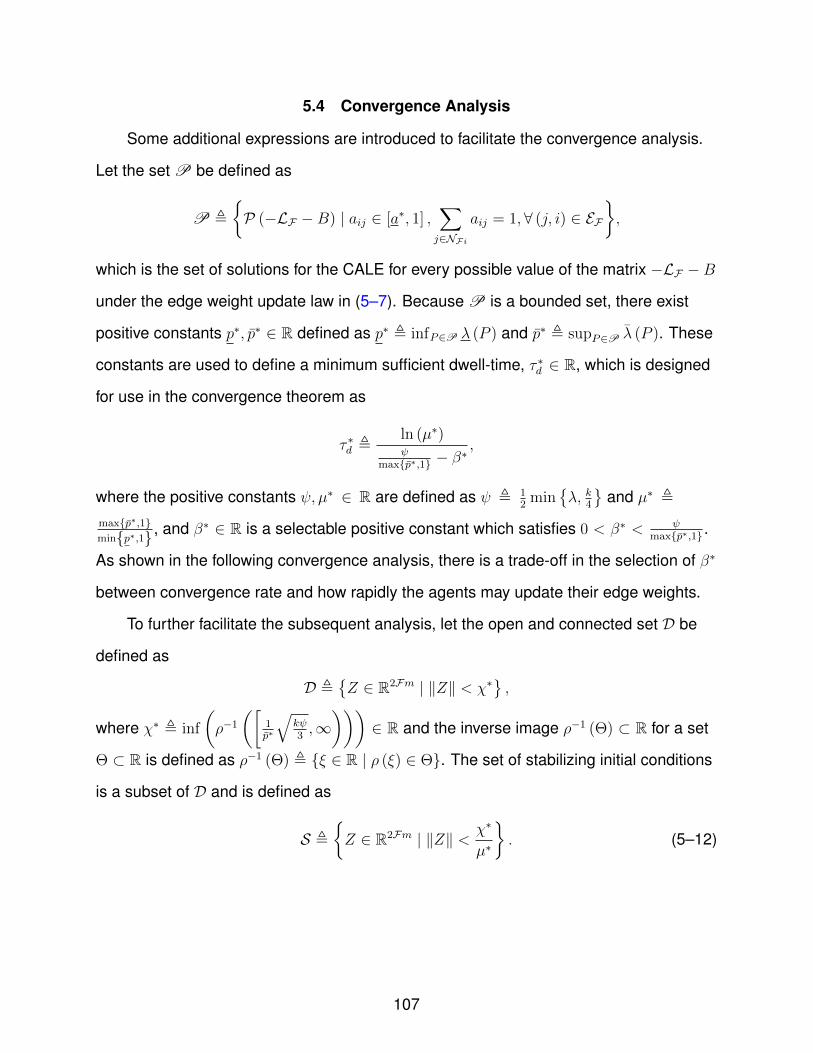
5.4 Convergence Analysis
Some additional expressions are introduced to facilitate the convergence analysis.
Let the set P be defined as
P ,
{P (−LF −B) | aij ∈ [a∗, 1] ,
∑j∈NFi
aij = 1, ∀ (j, i) ∈ EF},
which is the set of solutions for the CALE for every possible value of the matrix −LF − B
under the edge weight update law in (5–7). Because P is a bounded set, there exist
positive constants p∗, p∗ ∈ R defined as p∗ , infP∈P λ (P ) and p∗ , supP∈P λ (P ). These
constants are used to define a minimum sufficient dwell-time, τ ∗d ∈ R, which is designed
for use in the convergence theorem as
τ ∗d ,ln (µ∗)ψ
max{p∗,1} − β∗,
where the positive constants ψ, µ∗ ∈ R are defined as ψ , 12
min{λ, k
4
}and µ∗ ,
max{p∗,1}min{p∗,1} , and β∗ ∈ R is a selectable positive constant which satisfies 0 < β∗ < ψ
max{p∗,1} .
As shown in the following convergence analysis, there is a trade-off in the selection of β∗
between convergence rate and how rapidly the agents may update their edge weights.
To further facilitate the subsequent analysis, let the open and connected set D be
defined as
D ,{Z ∈ R2Fm | ‖Z‖ < χ∗
},
where χ∗ , inf
(ρ−1
([1p∗
√kψ3,∞)))
∈ R and the inverse image ρ−1 (Θ) ⊂ R for a set
Θ ⊂ R is defined as ρ−1 (Θ) , {ξ ∈ R | ρ (ξ) ∈ Θ}. The set of stabilizing initial conditions
is a subset of D and is defined as
S ,
{Z ∈ R2Fm | ‖Z‖ < χ∗
µ∗
}. (5–12)
107
Finally, the constant parameter LB ∈ R is defined as LB ,√|EF |+ F +
∑i∈VF b
2i , which
upper-bounds supt∈R ‖LF (t) +B‖ since ‖LF (t) +B‖ ≤ ‖LF (t) +B‖F ≤ LB for all t ∈ R
by the triangle inequality and the fact that 0 < aij ≤ 1, aii = 0 for all i, j ∈ VF .
The following theorem describes sufficient conditions for the approximate conver-
gence of the follower agents’ states towards the leader’s state under the decentralized
control policy in (5–4).
Theorem 5.1. The decentralized controller in (5–4) along with the edge weight update
policy in (5–7) provide UUB leader synchronization for a network of agents with nonlin-
ear dynamics described in (5–1) and neighbor communication and sensing feedback
described in Section 5.1.3 in the sense that lim supt→∞ ‖xi (t)− xL (t)‖ ≤ ε for some
ε ∈ R>0 and every follower agent i ∈ VF for all initial conditions Z (0) ∈ S, provided
that Assumptions 5.1-5.5 are satisfied, the dwell-time τd satisfies τd ≥ τ ∗d , and the state
estimate errors are sufficiently small such that there exists a selection for the gain k
which satisfies the inequality
3(p∗Nd
)2
k+ 3k
(p∗FLB (¯x+ λx)
)2<
ψχ∗
µ∗max {p∗, 1} . (5–13)
Remark 5.1. The inequality in (5–13) can be satisfied for sufficiently small estimate
error upper bounds x, ¯x; however, as intuition would indicate, stability is not guaranteed
for arbitrarily large estimate error upper bounds. Future research may overcome this
restriction by developing an algorithm which severs neighbor connections if the apparent
error in the communicated state estimates exceeds a threshold, i.e., aij 6= 0 if and only if
(j, i) ∈ EF and σij > σT , where σT ∈ (0, 1) is a threshold parameter.
Proof. Let the set {t0d, t1d, . . .} be defined as the union of the switching instances by each
agent, including the initial time, such that tl+1d > tld for all l ∈ Z≥0. Additionally, let the
mapping Λ : [0,∞)→ Z≥0 be defined such that Λ (t) is the number of switches that have
occurred until time t, i.e., Λ (t) , arg minl∈Z≥0
{t− tld | t− tld ≥ 0
}. A candidate multiple
108
Lyapunov function, VL : D × R→ R, is defined as
VL (Z, t) , WΛ(t) (Z) ,
where the function Wl : D → R belongs to a family of Lyapunov-like functions
{Wl | l ∈ Z≥0} defined as
Wl (Z) ,1
2ETE +
1
2RT(P(−LF
(tld)−B
)⊗ Im
)R,
which satisfies the inequalities
1
2min
{p∗, 1
}‖Z‖2 ≤ Wl (Z) ≤ 1
2max {p∗, 1} ‖Z‖2 (5–14)
for all Z ∈ R2Fm and l ∈ Z≥0. Using the closed-loop error system in (5–9), the derivative
of VL can be expressed as
VL =ET (R− λE) +RT(P(−LF
(tΛ(t)d
)−B
)⊗ Im
)·(Nd + N −
(P(−LF
(tΛ(t)d
)−B
)⊗ Im
)−1
E + k((−LF
(tΛ(t)d
)−B
)⊗ Im
)R
+ k((LF(tΛ(t)d
)+B
)⊗ Im
)(˙X − X + λ
(X −X
)))for all t ∈
[tld, t
l+1d
). After using the definitions of p∗, p∗, and LB, the relation
kRT ((P (−LF −B) (−LF −B))⊗ Im)R =k
2RT[(P (−LF −B) (−LF −B))⊗ Im
+(
(−LF −B)T P (−LF −B))⊗ Im
]R = −k
2‖R‖2 ,
the bounding expressions in (5–10) and (5–11), and canceling terms, VL can be upper-
bounded as
VL ≤− λ ‖E‖2 − k
2‖R‖2 + p∗Nd ‖R‖+ p∗ρ (‖Z‖) ‖Z‖ ‖R‖
+ kp∗LB∥∥∥ ˙X − X + λ
(X −X
)∥∥∥ ‖R‖
109
for all t ∈[tld, t
l+1d
). After some algebraic manipulation, VL can be upper-bounded as
VL ≤− λ ‖E‖2 − k
4‖R‖2 +
3(p∗Nd
)2
k+
3 (p∗ρ (‖Z‖) ‖Z‖)2
k
+ 3k(p∗LB
∥∥∥ ˙X − X + λ
(X −X
)∥∥∥)2
for all t ∈[tld, t
l+1d
). By using the definition of the auxiliary constant ψ, Assumption 5.4,
and the triangle inequality, VL is then upper-bounded as
VL ≤ −ψ ‖Z‖2 −(ψ − 3 (p∗ρ (‖Z‖))2
k
)‖Z‖2 + ε1
for all t ∈[tld, t
l+1d
), where the constant ε1 ∈ R is defined as ε1 ,
3(p∗Nd)2
k+
3k(p∗FLB (¯x+ λx)
)2. Provided the initial condition satisfies Z (0) ∈ S, then
VL ≤ −ψ ‖Z‖2 + ε1
for all t ∈[tld, t
l+1d
). By using the right-side inequality in (5–14), the upper bound of VL
can be expressed as
VL ≤−ψ
max {p∗, 1}VL −(
ψ
max {p∗, 1}VL − ε1
)≤− ψ
max {p∗, 1}VL ∀VL ≥max {p∗, 1}
ψε1 (5–15)
for all t ∈[tld, t
l+1d
). Using the comparison lemma (cf. [76, Lemma 3.4]) with the
inequality in (5–15), VL can be shown to be upper-bounded as
VL (Z, t) ≤ max
{e−
ψmax{p∗,1}(t−tld)VL
(Z(tld), tld),max {p∗, 1}
ψε1
}(5–16)
for all t ∈[tld, t
l+1d
). By using (5–16), the ultimate bound of the trajectory of VL can be
determined by considering the following three cases, where the constant ε2 ∈ R is
defined as ε2 , max{p∗,1}ψ
ε1 and Br ⊂ R2Fm denotes a closed ball of radius r ∈ R>0
centered about the origin.
Case 1: The trajectory of VL has not entered Bε2.
110
Consider that at time t′ ∈[tld, t
l+1d
), {VL (Z, t) | t ≤ t′} ∩ Bε2 = ∅. The inequality in
(5–16) can be conservatively upper-bounded to account for the effects of switches as
VL (Z (t′) , t′) ≤e−ψ(t′−tld)max{p∗,1}µ∗Wl−1
(Z(tld))
≤e−ψ(t′−tld)max{p∗,1}µ∗e−
ψ(tld−tl−1d )
max{p∗,1} Wl−1
(Z(tl−1d
))≤ · · ·
≤e−ψt′
max{p∗,1} (µ∗)lW0 (Z (0)) . (5–17)
By use of a minimum dwell-time, (5–17) may be upper-bounded as
VL (Z (t′) , t′) ≤ e−β∗t′W0 (Z (0)) (5–18)
if the dwell-time between switching events is greater than or equal to τ ∗d . Given (5–16)
and (5–18), it is clear that use of a dwell-time τd ≥ τ ∗d guarantees that VL is upper-
bounded by an exponential decay from the initial condition VL (Z (0) , 0) towards Bε2 for
any t′ ∈[tld, t
l+1d
)such that {VL (Z, t) | t ≤ t′} ∩Bε2 = ∅.
Case 2: The trajectory of VL has reached, or started in, the ball Bε2, and no switch has
occurred since entering Bε2.
Consider that VL (Z (t′) , t′) ∈ Bε2 at a time t′ ∈[tld, t
l+1d
). Then by (5–16), VL (Z, t) ∈
Bε2 for all t ∈[tld, t
l+1d
).
Case 3: The trajectory of VL was in the ball Bε2, and then a switch occurred.
Consider that the trajectory of VL was inside the ball Bε2 the instant before a
switch occurred at time tld. The Lyapunov function VL can only increase so much such
that VL(Z(tld), tld)∈ Bµ∗ε2 by the definition of µ∗, i.e.,
Wl(Z(tld),tld)Wl−1(Z(tld),tld)
≤ µ∗. Using the
definition of the dwell-time τ ∗d , it can be shown that Wl
(Z(tld + τ ∗d
), tld + τ ∗d
)≤ ε2, i.e., the
trajectory of VL re-enters the ball Bε2 before the next switching instance.
Thus, Cases 1-3 together imply that lim supt→∞ VL (Z, t) ≤ µ∗ε2, where the in-
equality in (5–13) guarantees that Bµ∗ε2 is contained within the set D. Therefore,
111
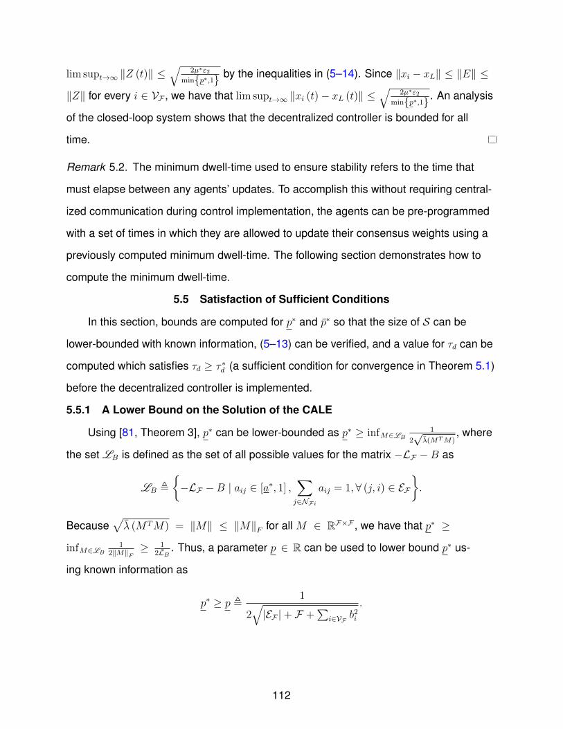
lim supt→∞ ‖Z (t)‖ ≤√
2µ∗ε2min{p∗,1} by the inequalities in (5–14). Since ‖xi − xL‖ ≤ ‖E‖ ≤
‖Z‖ for every i ∈ VF , we have that lim supt→∞ ‖xi (t)− xL (t)‖ ≤√
2µ∗ε2min{p∗,1} . An analysis
of the closed-loop system shows that the decentralized controller is bounded for all
time.
Remark 5.2. The minimum dwell-time used to ensure stability refers to the time that
must elapse between any agents’ updates. To accomplish this without requiring central-
ized communication during control implementation, the agents can be pre-programmed
with a set of times in which they are allowed to update their consensus weights using a
previously computed minimum dwell-time. The following section demonstrates how to
compute the minimum dwell-time.
5.5 Satisfaction of Sufficient Conditions
In this section, bounds are computed for p∗ and p∗ so that the size of S can be
lower-bounded with known information, (5–13) can be verified, and a value for τd can be
computed which satisfies τd ≥ τ ∗d (a sufficient condition for convergence in Theorem 5.1)
before the decentralized controller is implemented.
5.5.1 A Lower Bound on the Solution of the CALE
Using [81, Theorem 3], p∗ can be lower-bounded as p∗ ≥ infM∈LB
1
2√λ(MTM)
, where
the set LB is defined as the set of all possible values for the matrix −LF −B as
LB ,
{−LF −B | aij ∈ [a∗, 1] ,
∑j∈NFi
aij = 1,∀ (j, i) ∈ EF}.
Because√λ (MTM) = ‖M‖ ≤ ‖M‖F for all M ∈ RF×F , we have that p∗ ≥
infM∈LB
12‖M‖F
≥ 12LB
. Thus, a parameter p ∈ R can be used to lower bound p∗ us-
ing known information as
p∗ ≥ p ,1
2√|EF |+ F +
∑i∈VF b
2i
.
112
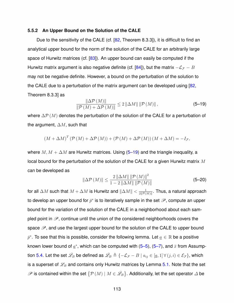
5.5.2 An Upper Bound on the Solution of the CALE
Due to the sensitivity of the CALE (cf. [82, Theorem 8.3.3]), it is difficult to find an
analytical upper bound for the norm of the solution of the CALE for an arbitrarily large
space of Hurwitz matrices (cf. [83]). An upper bound can easily be computed if the
Hurwitz matrix argument is also negative definite (cf. [84]), but the matrix −LF − B
may not be negative definite. However, a bound on the perturbation of the solution to
the CALE due to a perturbation of the matrix argument can be developed using [82,
Theorem 8.3.3] as‖∆P (M)‖
‖P (M) + ∆P (M)‖ ≤ 2 ‖∆M‖ ‖P (M)‖ , (5–19)
where ∆P (M) denotes the perturbation of the solution of the CALE for a perturbation of
the argument, ∆M , such that
(M + ∆M)T (P (M) + ∆P (M)) + (P (M) + ∆P (M)) (M + ∆M) = −IF ,
where M,M + ∆M are Hurwitz matrices. Using (5–19) and the triangle inequality, a
local bound for the perturbation of the solution of the CALE for a given Hurwitz matrix M
can be developed as
‖∆P (M)‖ ≤ 2 ‖∆M‖ ‖P (M)‖2
1− 2 ‖∆M‖ ‖P (M)‖ (5–20)
for all ∆M such that M + ∆M is Hurwitz and ‖∆M‖ < 12‖P(M)‖ . Thus, a natural approach
to develop an upper bound for p∗ is to iteratively sample in the set P, compute an upper
bound for the variation of the solution of the CALE in a neighborhood about each sam-
pled point in P, continue until the union of the considered neighborhoods covers the
space P, and use the largest upper bound for the solution of the CALE to upper bound
p∗. To see that this is possible, consider the following lemma. Let a ∈ R be a positive
known lower bound of a∗, which can be computed with (5–5), (5–7), and x from Assump-
tion 5.4. Let the set LB be defined as LB , {−LF −B | aij ∈ [a, 1]∀ (j, i) ∈ EF}, which
is a superset of LB and contains only Hurwitz matrices by Lemma 5.1. Note that the set
P is contained within the set{P (M) |M ∈ LB
}. Additionally, let the set operator ∆ be
113
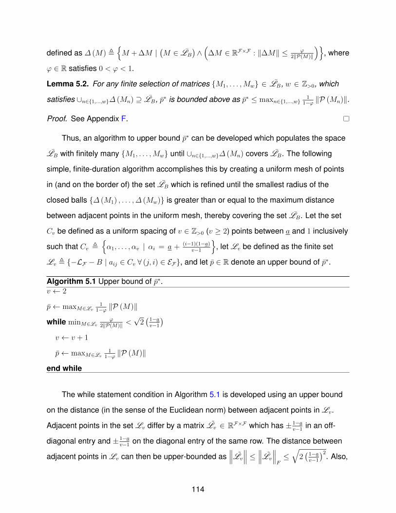
defined as ∆ (M) ,{M + ∆M |
(M ∈ LB
)∧(
∆M ∈ RF×F : ‖∆M‖ ≤ ϕ2‖P(M)‖
)}, where
ϕ ∈ R satisfies 0 < ϕ < 1.
Lemma 5.2. For any finite selection of matrices {M1, . . . ,Mw} ∈ LB, w ∈ Z>0, which
satisfies ∪n∈{1,...,w}∆ (Mn) ⊇ LB, p∗ is bounded above as p∗ ≤ maxn∈{1,...,w}1
1−ϕ ‖P (Mn)‖.
Proof. See Appendix F.
Thus, an algorithm to upper bound p∗ can be developed which populates the space
LB with finitely many {M1, . . . ,Mw} until ∪n∈{1,...,w}∆ (Mn) covers LB. The following
simple, finite-duration algorithm accomplishes this by creating a uniform mesh of points
in (and on the border of) the set LB which is refined until the smallest radius of the
closed balls {∆ (M1) , . . . , ∆ (Mw)} is greater than or equal to the maximum distance
between adjacent points in the uniform mesh, thereby covering the set LB. Let the set
Cv be defined as a uniform spacing of v ∈ Z>0 (v ≥ 2) points between a and 1 inclusively
such that Cv ,{α1, . . . , αv | αi = a + (i−1)(1−a)
v−1
}, let Lv be defined as the finite set
Lv , {−LF −B | aij ∈ Cv ∀ (j, i) ∈ EF}, and let p ∈ R denote an upper bound of p∗.
Algorithm 5.1 Upper bound of p∗.v ← 2
p← maxM∈Lv
11−ϕ ‖P (M)‖
while minM∈Lv
ϕ2‖P(M)‖ <
√2(
1−av−1
)v ← v + 1
p← maxM∈Lv
11−ϕ ‖P (M)‖
end while
The while statement condition in Algorithm 5.1 is developed using an upper bound
on the distance (in the sense of the Euclidean norm) between adjacent points in Lv.
Adjacent points in the set Lv differ by a matrix Lv ∈ RF×F which has ±1−av−1
in an off-
diagonal entry and ±1−av−1
on the diagonal entry of the same row. The distance between
adjacent points in Lv can then be upper-bounded as∥∥∥Lv
∥∥∥ ≤ ∥∥∥Lv
∥∥∥F≤√
2(
1−av−1
)2. Also,
114

note that a larger selection of the parameter ϕ can decrease the number of iterations in
Algorithm 5.1, but this may result in a more conservative upper bound for p∗. While this
algorithm theoretically terminates in finite operations, it may require too many operations
to be feasibly run for a large-sized network. Algorithm 5.1 is only shown for proof of
concept; for actual implementation, a more sophisticated optimization routine may be
developed from Algorithm 5.1, or a more traditional optimization technique can be used
to approximate p∗ or max{P (M) |M ∈ LB
}.
5.5.3 Computation of Sufficient Conditions
With the bounding constants p and p that satisfy p ≤ p∗ and p ≥ p∗, the size of the
set of stabilizing initial conditions S can be lower bounded and satisfaction of (5–13)
and τd ≥ τ ∗d can be guaranteed. Specifically, a conservative estimate S ⊆ S can be
computed as
S ,
{Z ∈ R2Fm | ‖Z‖ < χ
µ
},
where the constants χ, µ ∈ R are defined as χ , inf
(ρ−1
([1p
√kψ3,∞)))
∈ R and
µ , max{p,1}min{p,1} . Additionally, (5–13) is satisfied if the following computable condition is
satisfied
3(pNd
)2
k+ 3k
(pFLB (¯x+ λx)
)2<
ψχ
µmax {p, 1} .
Finally, τd can be selected such that
τd =ln (µ)ψ
max{p,1} − β,
where the tuning parameter β ∈ R is selected such that 0 < β < ψmax{p,1} . The inequality
τd ≥ τ ∗d is clearly satisfied if β∗ is assigned as β∗ = β. As with β∗, the selection of β
involves a trade-off between convergence rate and the frequency of an agent’s edge
weight updates.
115

Note that the methods used to compute the bounds p and p in Sections 5.5.1 and
5.5.2 produce conservative estimates. More sophisticated optimization approaches may
yield less conservative bounds and take less computational resources.
5.6 Simulation
The performance of the consensus weight update law given in (5–5)-(5–7) with the
controller in (5–4) is demonstrated using the four-agent network depicted if Fig. 5-1 and
the heterogeneous nonlinear dynamics
xi =
κi sin (xi,2) xi,2 κi sin (xi,2) (xi,1 + xi,2)
−κi sin (xi,2) xi,1 0
xi − υ1,i 0
0 υ2,i
xi + ui,
where the constant parameters κi, υ1,i, υ2,i ∈ R are described in Table 5-1 and x1,i, x2,i
respectively denote the first and second entries of the vector xi. The only nonzero
pinning gain is selected as b1 = 3 and the control gains are selected as k = 60, λ = 20.
The tuning parameter s and constant t, used in the trust metric in (5–5), are selected as
s = 1 and t = 10 s. The gains used in the reputation algorithm in (5–6) are selected as
ηζi = 10, ησi = 0.1 for all i ∈ VF . The simulation is meant to model a real-world scenario
in that it is anticipated that the trust values will be lower-bounded as σij ≥ 0.2 for all
i ∈ VF , j ∈ NFi, which, as previously mentioned, implies that ζij ≥ 0.2 for all i ∈ VF ,
j ∈ NFi. The MATLAB optimization routine fmincon is executed to obtain estimates of
p∗ and p∗ using the gains k and λ, the network topology depicted in Fig. 5-1, the pinning
gain b1, and the bounds 0.2 ≤ ζij ≤ 1, resulting in the estimates p = 0.119 and p = 8.28.
The dwell-time for the consensus weight updates is then computed as τd = 2.4 s using
the assignment β = 0.001 2ψmax{p,1} . The agents’ onboard sensor equipment is modeled
to have a frequency of 20 Hz, where at each sensor measurement an agent has a 50%
chance of sensing a neighbor. Only one neighbor can be observed in a single sensor
measurement, and the neighbor seen is a random selection, where each neighbor is
equally likely to be seen. The onboard position estimates are modeled to be affected by
116

an offset such that xi = xi+ ∆xi, where ∆x1 =
1
1
, ∆x2 =
−1
−1
, ∆x3 =
0.5
sin (t)
,
and
∆x4 =
−0.5
−0.5
if t < 60
(90 + 30 sin (7t))
1
1
if t ≥ 60.
Thus, agents 1-4 have very accurate (but not perfect) estimates of their position from
0− 60 s. After 60 s, the position estimate maintained by agent 4 becomes very inaccurate,
which may be due to onboard localization sensor failure, for example. The onboard
velocity estimates are similarly affected as ˙xi = xi +ddt
(∆xi). The network-wide objective
is to track the leader state trajectory, which evolves as xL =
sin (t)
0.5 cos (t)
.
To demonstrate the benefit of updating the consensus weights based on reputation,
consensus weights are updated after the closed-loop system has come to steady-
state. The first update occurs at 120 s and the agents’ updates are staggered in time in
intervals of τd. The benefit of the consensus weight updates is shown in the plot of the
leader-tracking error in Fig. 5-2, where the leader-tracking error of agent 4 is high due to
its very inaccurate state estimate, and is therefore omitted. The tracking error of agent 1
is less affected by the inaccurate position and velocity estimates of agent 4 since agent
1 is directly connected to the leader; however, the effects of agent 4 percolate through
the network and severely worsen the tracking performance of agents 2 and 3, as shown
in Fig. 5-2. The deleterious effects of agent 4 are mitigated by the trust measurements,
neighbor reputations, and consensus weight updates, shown in Fig. 5-3 - 5-5. Upon
achieving steady-state using consensus weight updates, the leader-tracking errors
return to values similar to those obtained when agent 4 had very accurate position
estimates. The RMS leader-tracking performance for agents 1 − 3 is quantified in
117
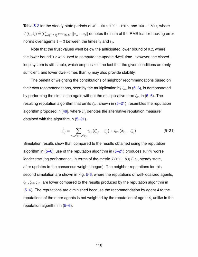
Table 5-2 for the steady-state periods of 40 − 60 s, 100 − 120 s, and 160 − 180 s, where
J (t1, t2) ,∑
i∈{1,2,3} rms[t1,t2] ‖xL − xi‖ denotes the sum of the RMS leader-tracking error
norms over agents 1− 3 between the times t1 and t2.
Note that the trust values went below the anticipated lower bound of 0.2, where
the lower bound 0.2 was used to compute the update dwell-time. However, the closed-
loop system is still stable, which emphasizes the fact that the given conditions are only
sufficient, and lower dwell-times than τd may also provide stability.
The benefit of weighting the contributions of neighbor recommendations based on
their own recommendations, seen by the multiplication by ζin in (5–6), is demonstrated
by performing the simulation again without the multiplicative term ζin in (5–6). The
resulting reputation algorithm that omits ζin, shown in (5–21), resembles the reputation
algorithm proposed in [49], where ζ ′ij denotes the alternative reputation measure
obtained with the algorithm in (5–21).
ζ ′ij =∑
n∈NFi∩NFj
ηζi(ζ ′nj − ζ ′ij
)+ ησi
(σij − ζ ′ij
)(5–21)
Simulation results show that, compared to the results obtained using the reputation
algorithm in (5–6), use of the reputation algorithm in (5–21) produces 10.7% worse
leader-tracking performance, in terms of the metric J (160, 180) (i.e., steady state,
after updates to the consensus weights began). The neighbor reputations for this
second simulation are shown in Fig. 5-6, where the reputations of well-localized agents,
ζ21, ζ32, ζ13, are lower compared to the results produced by the reputation algorithm in
(5–6). The reputations are diminished because the recommendation by agent 4 to the
reputations of the other agents is not weighted by the reputation of agent 4, unlike in the
reputation algorithm in (5–6).
118

Figure 5-1. Network communication topology.
Agent 1 2 3 4
κi 0.3 0.7 0.5 0.9
υ1,i 5.0 5.5 4.5 4.0
υ2,i 1.0 0.5 0.7 1.2
Table 5-1. Parameters in dynamics.
J (40, 60) 4.64
J (100, 120) 8.68
J (160, 180) 4.30
Table 5-2. Steady-state RMS leader-tracking performance.
119
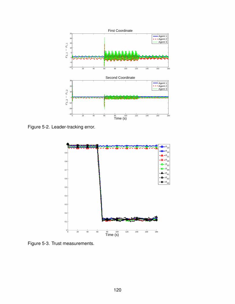
0 20 40 60 80 100 120 140 160 180−10
−5
0
5
10
15
20
25
xL,1−
xi,1
First Coordinate
Agent 1Agent 2Agent 3
0 20 40 60 80 100 120 140 160 180−30
−20
−10
0
10
20
30
Time (s)
xL,2−
xi,2
Second Coordinate
Agent 1Agent 2Agent 3
Figure 5-2. Leader-tracking error.
0 20 40 60 80 100 120 140 160 1800
0.1
0.2
0.3
0.4
0.5
0.6
0.7
0.8
0.9
1
Time (s)
σ
13
σ14
σ21
σ24
σ32
σ34
σ41
σ42
σ43
Figure 5-3. Trust measurements.
120
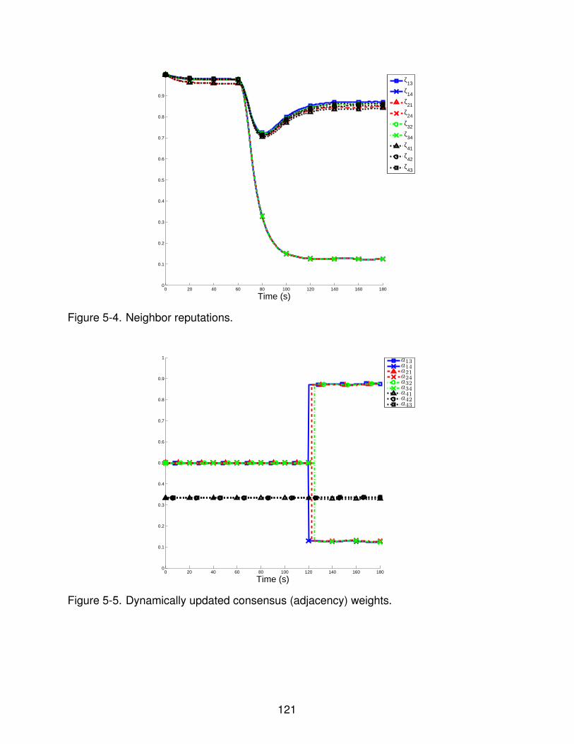
0 20 40 60 80 100 120 140 160 1800
0.1
0.2
0.3
0.4
0.5
0.6
0.7
0.8
0.9
1
Time (s)
ζ
13
ζ14
ζ21
ζ24
ζ32
ζ34
ζ41
ζ42
ζ43
Figure 5-4. Neighbor reputations.
0 20 40 60 80 100 120 140 160 1800
0.1
0.2
0.3
0.4
0.5
0.6
0.7
0.8
0.9
1
Time (s)
a13a14a21a24a32a34a41a42a43
Figure 5-5. Dynamically updated consensus (adjacency) weights.
121
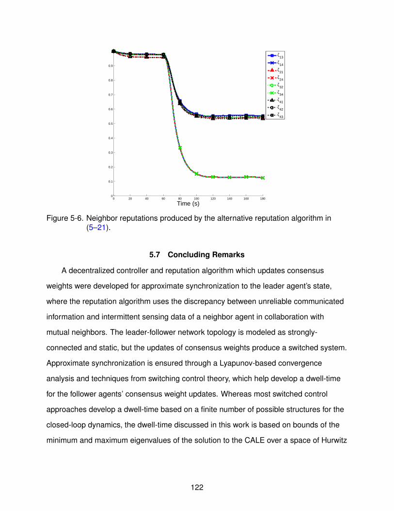
0 20 40 60 80 100 120 140 160 1800
0.1
0.2
0.3
0.4
0.5
0.6
0.7
0.8
0.9
1
Time (s)
ζ
13
ζ14
ζ21
ζ24
ζ32
ζ34
ζ41
ζ42
ζ43
Figure 5-6. Neighbor reputations produced by the alternative reputation algorithm in(5–21).
5.7 Concluding Remarks
A decentralized controller and reputation algorithm which updates consensus
weights were developed for approximate synchronization to the leader agent’s state,
where the reputation algorithm uses the discrepancy between unreliable communicated
information and intermittent sensing data of a neighbor agent in collaboration with
mutual neighbors. The leader-follower network topology is modeled as strongly-
connected and static, but the updates of consensus weights produce a switched system.
Approximate synchronization is ensured through a Lyapunov-based convergence
analysis and techniques from switching control theory, which help develop a dwell-time
for the follower agents’ consensus weight updates. Whereas most switched control
approaches develop a dwell-time based on a finite number of possible structures for the
closed-loop dynamics, the dwell-time discussed in this work is based on bounds of the
minimum and maximum eigenvalues of the solution to the CALE over a space of Hurwitz
122

matrices due to the infinite number of possible combinations of the network consensus
weights.
123
CHAPTER 6CONCLUSIONS AND FUTURE WORK
6.1 Conclusions
Decentralized control is a powerful control technique which provides a means
for accomplishing an objective using a disaggregated, cooperating collection of au-
tonomous agents, such as teams of UAVs or AUVs performing reconnaissance, satel-
lites performing collective interferometry, and platoons of ground robots. Delegating a
collective task to multiple systems provides benefits in terms of lower communication
bandwidth, robustness to hardware failure, increased strategic flexibility, and spatial dis-
tribution. However, the benefits of the distribution of mission planning and execution to
individual autonomous systems are accompanied by the disadvantage of less situational
awareness: the networked systems are only aware of the status of network neighbors
in a decentralized communication architecture. Among other consequences, this phe-
nomena makes decentralized multi-agent networks more susceptible to cascading,
destabilizing effects caused by exogenous disturbances on an agent’s plant or control
system, communication delay between network neighbors, and reduced ability to vet the
accuracy of communicated information. This dissertation addresses these challenges
through the development of novel decentralized control techniques that restrict the
propagation of these deleterious effects through the network of autonomous systems.
Chapter 2 details the development of a novel decentralized controller which ad-
dresses the challenge of mitigating the effects of exogenous disturbances in a network
of autonomous systems while performing synchronization, wherein agents share in-
formation with network neighbors in an attempt to collectively drive all agents’ states
towards that of a network leader. The exogenous disturbances are assumed to be
unknown and represent the effects of unmodeled dynamics and external force effects on
an agent’s dynamics (e.g., a gust of wind causes undesired movement of a UAV). The
agents’ dynamics are modeled with heterogeneous Euler-Lagrange equations of motion
124

due to broad applicability to physical systems. Concepts from the RISE control tech-
nique and graph theory are leveraged in the development of the decentralized controller
and the proof of asymptotic convergence of the agent’s states to that of the network
leader’s. In the proof of convergence, it is demonstrated that the developed controller
compensates for the effects of the disturbances of all agents using only relative state
information. Simulation results are given which demonstrate the enhanced performance
of the developed controller compared to other prominent decentralized controllers.
The developed controller is then extended from the synchronization framework to the
formation control framework, wherein the agents converge to a geometric configuration
specified by desired relative positions between the agents.
The decentralized control technique in Chapter 2 is generalized in Chapter 3 for
the objective of containment control. As opposed to synchronization, in which a single
leader interacts with the follower agents, the objective of containment control is to
have the autonomous follower agents cooperatively interact with multiple leaders and
converge to a reasonable linear combination of the leaders’ states. For example, a flock
of autonomous UAVs may be guided by multiple remotely piloted UAVs in performing
a search mission. Specifically, containment control specifies that the follower agents’
states converge to the convex hull demarcated by the states of the leaders. Again,
concepts from the RISE control technique and graph theory are used to demonstrate
convergence of the follower agents’ states to the convex hull of the leaders’ dynamic
states despite the effects of modeling uncertainty and exogenous disturbances.
The developments in Chapter 4 address compensation for the effects of commu-
nication delay in a decentralized network in which the agents have heterogeneous, un-
certain Euler-Lagrange dynamics and heterogeneous, uncertain communication delays.
Communication delay drastically affects performance in accomplishing a network-wide
objective, such as synchronization, since the effect of a change in a network leader’s
state may not impact a follower agent until multiple periods of delay have passed as
125
the change percolates through the network. In Chapter 4, the notions of self-delayed
feedback and feedback without self-delay are introduced: self-delayed feedback signifies
the comparison of a neighbor’s delayed state with an agent’s own manually delayed
state, and feedback without self delay signifies the comparison of a neighbor’s delayed
state with an agent’s own current state. The advantages and disadvantages of both
feedback types are exemplified in a simulation and a novel decentralized controller is
developed which uses both of these types of feedback and estimates of what neighbors’
communication delay durations are. A numerical simulation demonstrates that a mixture
of these two types of feedback can provide enhanced stability criteria and improved
leader-tracking for the synchronization framework.
Chapter 5 addresses the issue of diminished situational awareness in a decen-
tralized interaction environment by developing a control architecture to enhance the
robustness of decentralized control to the communication of inaccurate state informa-
tion. Assuming that communicated information is continuously available, but possibly
inaccurate, and that neighbor sensing is intermittent, yet accurate, a trust metric is
developed that quantifies the accuracy and reliability of a neighbor’s communication.
Trust values are shared via a neighborhood-based reputation algorithm, wherein agents
collaborate to develop a reputation of a mutual neighbor and reputation recommen-
dations are weighted by the reputation of the recommender. Neighbor reputations are
used to weigh the communicated feedback from neighbors in a decentralized control
policy by adjusting consensus weights as a function of neighbors’ reputations. Although
the network connections are modeled as static, updates to the consensus weights
introduce discontinuities into the closed-loop system. Notions from switching control
theory and the sensitivity of the CALE are used to develop a dwell-time for the follower
agents’ consensus weight updates through a Lyapunov-based convergence analy-
sis. Simulation results demonstrate that intermittent neighbor sensing can be used
126
to augment a communication-based control policy by vetting network neighbors in a
recommendation-based approach.
6.2 Future Work
The developments given in this dissertation have been shown to theoretically satisfy
control objectives and provide comparatively improved performance via Lyapunov-based
convergence analyses and numerical simulations. Justifications of these claims could
be further established if physical experiments were performed to demonstrate the real-
world applicability of the developed techniques. Ground vehicles or quadcopters may be
used in the future to demonstrate the efficacy of the control techniques detailed in this
dissertation.
Chapters 2-4 assume that the communication topology of the follower agents is
undirected. One avenue for extending this work would be to consider a communication
topology which is directed, i.e., not all communication links may be bidirectional. An
approach similar to that used in Chapter 5 may be used to approach this problem,
wherein the sum of the Laplacian matrix corresponding to the follower agent topology
and the leader-pinning matrix is used as an input to the Lyapunov equation, the solution
of which is a matrix that can be used to generate a candidate Lyapunov function.
However, this approach is complicated if considering Euler-Lagrange dynamics, which
cause an inertia matrix to be multiplied by the matrix solution of the Lyapunov equation
in the feedback expressions of the derivative of the candidate Lyapunov function.
Even though the matrix solution of the Lyapunov equation and the inertia matrix are
positive definite, it is not necessarily the case that the matrix product is positive definite,
which causes the feedback in the derivative of the candidate Lyapunov function to
be sign indefinite, and causes analysis with the candidate Lyapunov function to be
fruitless. This technical challenge could possibly be addressed by using the inertia
matrix in a controller to cancel the respective effects, but such a controller requires exact
127
model knowledge of the inertia matrix. Further research may provide insight in how to
guarantee compensation of dynamics’ inertia in general directed networks.
The decentralized controller developed in Chapter 4 addresses compensation
of the effects of communication delay by weighting the contributions of self-delayed
feedback and feedback without self-delay. This control technique may be enhanced by
additions such as developing time-varying feedback weights based on estimates of the
current communication delay, weighting feedback more for neighbors which have less
communication delay, a protocol which severs a neighbor connection if that neighbor’s
large communication delay makes its feedback only deleterious, and developing a
decentralized estimator of the network leader’s state so that the cascading effect of
communication delay has less impact.
Some exciting results may be extended from the developments in Chapter 5. In
particular, these developments can be extended to devise more sophisticated context-
dependent reputation algorithms, an augmentation to the decentralized controller which
decides when to sever neighbor connections, and an observer which determines a more
accurate estimate of neighbors’ states given unreliable communication and intermittent
sensing.
128

APPENDIX APROOF THAT P IS NONNEGATIVE (CH 2)
Lemma A.1. Given the differential equation in (2–23), P ≥ 0 if, for all i ∈ VF , χi satisfies
χi > ‖ςai‖∞ +1
α2,i
‖ςbi‖∞ . (A–1)
Proof. For notational brevity, let an auxiliary signal σ ∈ R be the negative of the integral
of P in (2–23) as
σ =
tˆ
0
ET2 (ε) Λ2 (Nd (ε)− β sgn (E2 (ε))) dε+
tˆ
0
∂ET2 (ε)
∂εNd (ε) dε
−tˆ
0
∂ET2 (ε)
∂εβ sgn (E2 (ε)) dε. (A–2)
Integrating the last two terms in (A–2) yields [58, Lemma 1]
σ =
tˆ
0
ET2 (ε) Λ2 (Nd (ε)− β sgn (E2 (ε))) dε+
Fm∑l=1
E2l (t)Ndl (t)− ET2 (0)Nd (0)
−tˆ
0
ET2 (ε)
∂Nd (ε)
∂εdε−
Fm∑l=1
|E2l (t)| βl,l +Fm∑l=1
|E2l (0)| βl,l. (A–3)
The expression in (A–3) may then be expressed as
σ =
tˆ
0
(Fm∑l=1
E2l (ε) Λ2l,lNdl (ε)
)dε−
tˆ
0
(Fm∑l=1
|E2l (ε)|Λ2l,lβl,l
)dε
−tˆ
0
(Fm∑l=1
E2l (ε) Ndl (ε)
)dε+
Fm∑l=1
E2l (t)Ndl (t)− ET2 (0)Nd (0)
−Fm∑l=1
|E2l (t)| βl,l +Fm∑l=1
|E2l (0)| βl,l. (A–4)
129
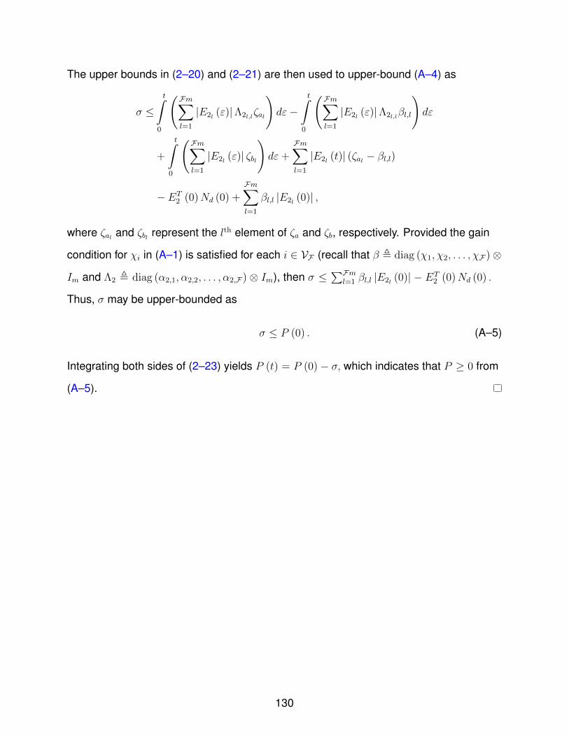
The upper bounds in (2–20) and (2–21) are then used to upper-bound (A–4) as
σ ≤tˆ
0
(Fm∑l=1
|E2l (ε)|Λ2l,lζal
)dε−
tˆ
0
(Fm∑l=1
|E2l (ε)|Λ2l,lβl,l
)dε
+
tˆ
0
(Fm∑l=1
|E2l (ε)| ζbl
)dε+
Fm∑l=1
|E2l (t)| (ζal − βl,l)
− ET2 (0)Nd (0) +
Fm∑l=1
βl,l |E2l (0)| ,
where ζal and ζbl represent the lth element of ζa and ζb, respectively. Provided the gain
condition for χi in (A–1) is satisfied for each i ∈ VF (recall that β , diag (χ1, χ2, . . . , χF)⊗
Im and Λ2 , diag (α2,1, α2,2, . . . , α2,F) ⊗ Im), then σ ≤ ∑Fml=1 βl,l |E2l (0)| − ET2 (0)Nd (0) .
Thus, σ may be upper-bounded as
σ ≤ P (0) . (A–5)
Integrating both sides of (2–23) yields P (t) = P (0)− σ, which indicates that P ≥ 0 from
(A–5).
130
APPENDIX BPROOF OF SUPPORTING LEMMA (CH 3)
Proof of Lemma 3.1. Because the eigenvalues of LF + B are positive by
Assumption 3.5 and [18, Lemma 4.1], the diagonal entries are positive, and the
off-diagonal entries are nonpositive, all entries of the matrix (LF +B)−1 are non-
negative [85, Theorem 2.3]. Due to the structure of the Laplacian matrix L, we
have that L1F+L = 0F+L, which implies (LF +B)1F + LL1L = 0L. Because
LF + B is invertible, 1F = − (LF +B)−1 LL1L, which implies that row sums of
− (LF +B)−1 LL add to one, where each entry of the matrix − (LF +B)−1 LL is
nonnegative since (LF +B)−1 has only nonnegative entries and LL has only non-
positive entries. Thus, the product −((
(LF +B)−1 LL)⊗ Im
)QL can be represented
as[qTd1, . . . , qTdF
]T= −
(((LF +B)−1 LL
)⊗ Im
)QL ∈ RFm, where qdi ∈ Rm
such that qdi =∑
l∈{1,...,L}[− (LF +B)−1 LL
]ilql ∀i ∈ {1, . . . ,F}, where [·]ij denotes
the matrix entry of the ith row and jth column,∑
l∈{1,...,L}[− (LF +B)−1 LL
]il
= 1
∀i ∈ {1, . . . ,F}, and[− (LF +B)−1 LL
]il≥ 0 ∀i ∈ {1, . . . ,F} ,∀l ∈ {1, . . . , L} by
the above conclusions. Because the convex hull for the set S , {ql | l ∈ VL} is de-
fined as Conv {S} ,{∑
l∈VL αlql | (∀l : R 3 αl ≥ 0) ∧∑l∈VL αl = 1}
[86], we have
that qdi ∈ Conv {ql | l ∈ VL} ∀i ∈ {1, . . . ,F}; in other words, the vectors stacked in
the product −((
(LF +B)−1 LL)⊗ Im
)QL are within the convex hull formed with the
leader agents’ states. Suppose that ‖E1‖ → 0. Then∥∥((LF +B)⊗ Im)−1E1
∥∥ → 0,
which implies that∥∥QF +
(((LF +B)−1 LL
)⊗ Im
)QL
∥∥ → 0 by (3–4), and thus
QF =
[qTL+1, . . . , qTL+F
]T→ −
(((LF +B)−1 LL
)⊗ Im
)QL =
[qTd1, . . . , qTdF
]T.
Hence, d (qi,Conv {ql | l ∈ VL})→ 0 ∀i ∈ VF .
131

APPENDIX CDEMONSTRATION OF SUPPORTING INEQUALITY (CH 4)
Consider the inequality aT b ≤ 12ΦaTa + Φ
2bT b for any vectors a, b ∈ RFm and any
positive scalar Φ ∈ R>0. After setting aT = kRT (κ1Aij − κ2Lij), b =´ tt−τji R (σ) dσ, and
Φ = φ ι2τk2 , the scalar RTk
∑(j,i)∈EF (κ1Aij − κ2Lij)
´ tt−τji R (σ) dσ can be upper-bounded
as1
∑(j,i)∈EF
kRT (κ1Aij − κ2Lij)ˆ t
t−τjiR (σ) dσ ≤
∑(j,i)∈EF
(τ k2
2φι2k2RT (κ1Aij − κ2Lij) (κ1Aij − κ2Lij)T R
+φι2
2τ k2
(ˆ t
t−τjiRT (σ) dσ
)ˆ t
t−τjiR (σ) dσ
). (C–1)
By using the Raleigh-Ritz Theorem, (C–1) can be upper-bounded as
∑(j,i)∈EF
kRT (κ1Aij − κ2Lij)ˆ t
t−τjiR (σ) dσ ≤ τ k4
2φRTR
+φι2
2τ k2
∑(j,i)∈EF
(ˆ t
t−τjiRT (σ) dσ
)ˆ t
t−τjiR (σ) dσ. (C–2)
After using Assumption 4.6 and the inequality(´ b
0a (s) ds
)T (´ b0a (s) ds
)≤ b´ b
0aT (s) a (s) ds
for a ∈ RFm and b ∈ R>0, (C–2) can be upper-bounded as
∑(j,i)∈EF
kRT (κ1Aij − κ2Lij)ˆ t
t−τjiR (σ) dσ ≤ τ k4
2φRTR +
φι2 |EF |2k2
ˆ t
t−τ
∥∥∥R (σ)∥∥∥2
dσ.
1 Because any matrix product of the form ΞΞT is positive semi-definite for a squarereal matrix Ξ, the symmetric matrix
∑(j,i)∈EF (κ1Aij − κ2Lij) (κ1Aij − κ2Lij)T is positive
semi-definite. Additionally, since κ1Aij − κ2Lij has at least one nonzero entry for every(j, i) ∈ EF ,
∑(j,i)∈EF (κ1Aij − κ2Lij) (κ1Aij − κ2Lij)T does not have all zero entries. Since∑
(j,i)∈EF (κ1Aij − κ2Lij) (κ1Aij − κ2Lij)T is symmetric, positive semi-definite and not thezero matrix, we have that ι2 > 0.
132

The procedure for developing the remaining upper bounds given in (4–37) and (4–38) is
similar, and therefore omitted.
133

APPENDIX DDEMONSTRATION OF REPUTATION BOUND (CH 5)
Let the function ζ : R→ R be defined as
ζ (t) , min {ζij (t) | (j, i) ∈ EF} .
Suppose that (−∞, σ∗] ∩ {ζij (t) | t ≥ 0} 6= ∅ for some (j, i) ∈ EF , i.e., a repu-
tation value becomes less than or equal to σ∗ at some time. By continuity of ζij,
there exists some time T ∈ R>0 such that ζ (T ) = σ∗ > 0. Let Tσ be defined as
Tσ , min{t ∈ R | ζ (t) = σ∗
}. For any (h, g) ∈ EF such that ζgh (Tσ) = σ∗, we have that
ζgh (Tσ) =∑
n∈NFg∩NFh
ηζgζgn(ζnh − ζ
)+ ησg (σgh − σ∗) .
By the definition of ζ, we know that∑
n∈NFg∩NFh ηζgζgn(ζnh − ζ
)≥ 0. Additionally, by
the definition of σ∗, we know that ησg (σgh − σ∗) ≥ 0. Therefore, ζgh (Tσ) ≥ 0 and thus
ζgh (T+σ ) ≥ σ∗. By induction, ζij (t) ≥ σ∗ for all (j, i) ∈ EF and t ∈ R.
A similar argument shows that ζij (t) ≤ 1 for all (j, i) ∈ EF and t ∈ R based on the
facts that ζij (0) = 1 for all (j, i) ∈ EF and σij ≤ 1 for all (j, i) ∈ EF and t ∈ R.
134
APPENDIX EPROOF OF SUPPORTING LEMMA (CH 5)
Proof of Lemma 5.1. By Assumption 5.1 and [87, Lemma 4.6], the left eigenvector
p = [p1, . . . , pF ]T ∈ RF of LF associated with the (simple) zero eigenvalue has all
positive entries. Let ξ = [ξ1, . . . , ξF ]T ∈ RF \ {0F}. Because pTLF = 0F , we have that
pidi =∑F
j=1 pjaji, and hence∑F
j=1 piaij =∑F
j=1 pjaji for all i ∈ VF , which gives the
relation
F∑i=1
F∑j=1
piaijξi (ξi − ξj) =F∑i=1
F∑j=1
piaijξ2i −
F∑i=1
F∑j=1
piaijξiξj
=F∑i=1
F∑j=1
pjajiξ2i −
F∑i=1
F∑j=1
piaijξiξj
=F∑i=1
F∑j=1
piaijξ2j −
F∑i=1
F∑j=1
piaijξiξj
=F∑i=1
F∑j=1
piaijξj (ξj − ξi) . (E–1)
Let Q ∈ RF×F be defined as Q , P (LF +B)+(LF +B)T P , where P , diag {p1, . . . , pF} ∈
RF×F . The relation in (E–1) facilitates the expression of the product ξTQξ as
ξTQξ =ξTPLFξ + ξTLTFPξ + ξTPBξ + ξTBPξ
=2ξTPLFξ + 2ξTPBξ
=2F∑i=1
F∑j=1
piξiaij (ξi − ξj) + 2F∑i=1
pibiξ2i
=F∑i=1
F∑j=1
piaijξi (ξi − ξj) +F∑i=1
F∑j=1
piaijξj (ξj − ξi) + 2F∑i=1
pibiξ2i
=F∑i=1
F∑j=1
piaij (ξj − ξi)2 + 2F∑i=1
pibiξ2i .
Clearly, ξTQξ ≥ 0. Suppose that ξTQξ = 0 for some ξ ∈ RF \ {0F}, which requires
that∑F
i=1
∑Fj=1 piaij (ξj − ξi)2 = 0 and
∑Fi=1 pibiξ
2i = 0. Because GF is connected
and ξ ∈ RF \ {0F},∑F
i=1
∑Fj=1 piaij (ξj − ξi)2 = 0 if and only if ξ = α1F , where
135
α ∈ R \ {0}. However, if at least one follower agent is connected to the leader, then∑Fi=1 pibiξ
2i > 0 for all ξ ∈ span {1F} \ {0F}, which is a contradiction. Hence, ξTQξ > 0
for all ξ ∈ RF \ {0F}, i.e., Q is positive definite. Therefore, because P is positive definite
and symmetric and the matrix P (−LF −B) + (−LF −B)T P is negative definite by the
definition of Q, we have by [88, Theorem 8.2] that −LF −B is Hurwitz.
136
APPENDIX FPROOF OF SUPPORTING LEMMA (CH 5)
Proof of Lemma 5.2. Because sup{‖P (M)‖ |M ∈ LB
}is bounded, the ball ∆ (M)
is non-vanishing for any M ∈ LB. Additionally, because sup{‖P (M)‖ |M ∈ LB
}is
bounded, P is continuous in the non-vanishing neighborhood ∆ (M) ∩ LB for every
M ∈ LB by (5–20), which implies that P is continuous over LB. Hence, because P is
continuous over LB and LB is compact, the set{P (M) |M ∈ LB
}is compact, and
therefore there exists a matrix M0 ∈ LB such that ‖P (M)‖ ≤ ‖P (M0)‖ for every
M ∈ LB. Thus, for any finite selection of matrices {M1, . . . ,Mw} ∈ LB which satisfy
∪n∈{1,...,w}∆ (Mn) ⊇ LB, we have that
p∗ ≤‖P (M0)‖
≤ maxn∈{1,...,w}
max∆M∈∆(Mn)
(‖P (Mn + ∆M)‖)
= maxn∈{1,...,w}
max∆M∈∆(Mn)
(‖P (Mn) + ∆P (Mn)‖)
≤ maxn∈{1,...,w}
1
1− ϕ ‖P (Mn)‖
by the fact that P ⊂{P (M) |M ∈ LB
}, the definition of ∆ (·), the upper bound in
(5–20), and the triangle inequality. Note that ‖∆P (Mn)‖ is kept bounded by introducing
ϕ in the definition of ∆ to keep the denominator in (5–20) from being arbitrarily close to
zero.
137

REFERENCES
[1] G. Chen and F. L. Lewis, “Distributed adaptive tracking control for synchronizationof unknown networked Lagrangian systems,” IEEE Trans. Syst. Man Cybern.,vol. 41, no. 3, pp. 805–816, 2011.
[2] J. Mei and W. Ren, “Distributed coordinated tracking with a dynamic leader formultiple Euler-Lagrange systems,” IEEE Trans. Autom. Control, vol. 56, no. 6, pp.1415–1421, 2011.
[3] E. Nuno, R. Ortega, L. Basanez, and D. Hill, “Synchronization of networks of non-identical Euler-Lagrange systems with uncertian parameters and communicationdelays,” IEEE Trans. Autom. Control, vol. 56, no. 4, pp. 935–941, 2011.
[4] R. Olfati-Saber, J. A. Fax, and R. M. Murray, “Consensus problems in networksof agents with switching topology and time-delays,” IEEE Trans. Autom. Control,vol. 49, no. 9, pp. 1520–1533, 2004.
[5] E. Lavretsky, “F/A-18 autonomous formation flight control system design,” in AIAAConf. Guid., Navig., Control, 2002.
[6] J. Ploeg, A. F. Serrarens, and G. J. Heijenk, “Connect & drive: design and eval-uation of cooperative adaptive cruise control for congestion reduction,” J. Mod.Transp., vol. 19, no. 3, pp. 207–213, 2011.
[7] W. Ren, “Multi-vehicle consensus with a time-varying reference state,” Syst. ControlLett., vol. 56, pp. 474–483, 2007.
[8] A. Rodriguez-Angeles and H. Nijmeijer, “Mutual synchronization of robots viaestimated state feedback: A cooperative approach,” IEEE Trans. Control Syst.Technol., vol. 12, no. 4, pp. 542–554, 2004.
[9] S. Khoo and L. Xie, “Robust finite-time consensus tracking algorithm for multirobotsystems,” IEEE/ASME Trans. Mechatron., vol. 14, no. 2, pp. 219–228, 2009.
[10] S.-J. Chung and J.-J. E. Slotine, “Cooperative robot control and concurrent syn-chronization of Lagrangian systems,” IEEE Trans. on Robot., vol. 25, no. 3, pp.686–700, 2009.
[11] Y. Hong, J. Hu, and L. Gao, “Tracking control for multi-agent consensus with anactive leader and variable topology,” Automatica, vol. 42, no. 7, pp. 1177–1182,2006.
[12] Y. Hong, G. R. Chen, and L. Bushnell, “Distributed observers design for leaderfollowing control of multi-agent networks,” Automatica, vol. 44, no. 3, pp. 846–850,2008.
138
[13] D. V. Dimarogonas and K. H. Johansson, “Stability analysis for multi-agent systemsusing the incidence matrix: Quantized communication and formation control,”Automatica, vol. 46, no. 4, pp. 695–700, 2010.
[14] A. Abdessameud, I. G. Polushin, and A. Tayebi, “Synchronization of multiple Euler-Lagrange systems with communication delays,” in Proc. Am. Control Conf., June2012, pp. 3748–3753.
[15] Z. Li, W. Ren, X. Liu, and L. Xie, “Distributed consensus of linear multi-agentsystems with adaptive dynamic protocols,” Automatica, vol. 49, no. 7, pp. 1986–1995, 2013.
[16] H. Wang, “Passivity based synchronization for networked robotic systems withuncertain kinematics and dynamics,” Automatica, vol. 49, no. 3, pp. 755–761, 2013.
[17] J. Klotz, Z. Kan, J. M. Shea, E. L. Pasiliao, and W. E. Dixon, “Asymptotic synchro-nization of leader-follower networks of uncertain Euler-Lagrange systems,” in Proc.IEEE Conf. Decis. Control, Florence, IT, Dec. 2013, pp. 6536–6541.
[18] G. Notarstefano, M. Egerstedt, and M. Haque, “Containment in leader-followernetworks with switching communication topologies,” Automatica, vol. 47, no. 5, pp.1035–1040, 2011.
[19] D. V. Dimarogonas, P. Tsiotras, and K. J. Kyriakopoulos, “Leader-follower coop-erative attitude control of multiple rigid bodies,” Syst. Control Lett., vol. 58, pp.429–435, 2009.
[20] J. Mei, W. Ren, J. Chen, and G. Ma, “Distributed adaptive coordination for multipleLagrangian systems under a directed graph without using neighbors’ velocityinformation,” Automatica, vol. 49, no. 6, pp. 1723–1731, 2013.
[21] M. Ji, G. Ferrari-Trecate, M. Egerstedt, and A. Buffa, “Containment control in mobilenetworks,” IEEE Trans. Autom. Control, vol. 53, no. 8, pp. 1972–1975, 2008.
[22] Y. Cao, D. Stuart, W. Ren, and Z. Meng, “Distributed containment control formultiple autonomous vehicles with double-integrator dynamics: Algorithms andexperiments,” IEEE Trans. Control Syst. Technol., vol. 19, no. 4, pp. 929–938, 2011.
[23] J. Li, W. Ren, and S. Xu, “Distributed containment control with multiple dynamicleaders for double-integrator dynamics using only position measurements,” IEEETrans. Autom. Control, vol. 57, no. 6, pp. 1553–1559, 2012.
[24] Y. Cao, W. Ren, and M. Egerstedt, “Distributed containment control with multiplestationary or dynamic leaders in fixed and switching directed networks,” Automat-ica, vol. 48, pp. 1586–1597, 2012.
[25] Z. Kan, J. Klotz, E. L. Pasiliao, and W. E. Dixon, “Containment control for a directedsocial network with state-dependent connectivity,” in Proc. Am. Control Conf.,Washington DC, June 2013, pp. 1953–1958.
139
[26] Z. Meng, W. Ren, and Z. You, “Distributed finite-time attitude containment controlfor multiple rigid bodies,” Automatica, vol. 46, no. 12, pp. 2092–2099, 2010.
[27] J. Mei, W. Ren, and G. Ma, “Distributed containment control for Lagrangiannetworks with parametric uncertainties under a directed graph,” Automatica, vol. 48,no. 4, pp. 653–659, 2012.
[28] Z. Meng, D. V. Dimarogonas, and K. H. Johansson, “Zero-error coordinatedtracking of multiple Lagrange systems using continuous control,” in Proc. IEEEConf. Decis. Control, 2013, pp. 6712–6717.
[29] A. Abdessameud, I. G. Polushin, and A. Tayebi, “Synchronization of Lagrangiansystems with irregular communication delays,” IEEE Trans. Autom. Control, vol. 59,no. 1, pp. 187–193, 2014.
[30] A. Abdessameud and A. Tayebi, “Formation control of VTOL unmanned aerialvehicles with communication delays,” Automatica, vol. 47, pp. 2383–2394, 2011.
[31] N. Chopra, “Output synchronization on strongly connected graphs,” IEEE Trans.Autom. Control, vol. 57, no. 11, pp. 2896–2901, 2012.
[32] H. Li and Y. Shi, “Distributed receding horizon control of large-scale nonlinearsystems: Handling communication delays and disturbances,” Automatica, vol. 50,pp. 1264–1271, 2014.
[33] U. Munz, A. Papachristodoulou, and F. Allgower, “Delay robustness in non-identicalmulti-agent systems,” IEEE Trans. Autom. Control, vol. 57, no. 6, pp. 1597–1603,2012.
[34] Y.-P. Tian and C.-L. Liu, “Consensus of multi-agent systems with diverse input andcommunication delays,” IEEE Trans. Autom. Control, vol. 53, no. 9, pp. 2122–2128,2008.
[35] Y.-P. Tian and Y. Zhang, “High-order consensus of heterogeneous multi-agentsystems with unknown communication delays,” Automatica, vol. 48, pp. 1205–1212,2012.
[36] X. Wang, A. Saberi, A. A. Stoorvogel, H. F. Grip, and T. Yang, “Consensus in thenetwork with uniform constant communication delay,” Automatica, vol. 49, pp.2461–2467, 2013.
[37] H. Wang, “Consensus of networked mechanical systems with communicationdelays: A unified framework,” IEEE Trans. Autom. Control, vol. 59, no. 6, pp.1571–1576, 2014.
[38] B. Zhou and Z. Lin, “Consensus of high-order multi-agent systems with large inputand communication delays,” Automatica, vol. 50, pp. 452–464, 2014.
140
[39] Y.-C. Liu and N. Chopra, “Synchronization of networked mechanical systems withcommunication delays and human input,” ASME J. Dyn. Syst., Meas., and Control,vol. 135, no. 4, 2013.
[40] A. A. Peters, R. H. Middleton, and O. Mason, “Leader tracking in homogeneousvehicle platoons with broadcast delays,” Automatica, vol. 50, pp. 64–74, 2014.
[41] W. Zhu, “Consensus of multiagent systems with switching jointly reachable in-terconnection and time delays,” IEEE Trans. Syst., Man, Cybern. A, Syst., Hum.,vol. 42, no. 2, pp. 348–358, 2012.
[42] S. Liu, L. Xie, and F. L. Lewis, “Synchronization of multi-agent systems with delayedcontrol input information from neighbors,” Automatica, vol. 47, pp. 2152–2164,2011.
[43] K. Peng and Y. Yang, “Leader-following consensus problem with a varying-velocityleader and time-varying delays,” Physica A, vol. 388, pp. 193–208, 2009.
[44] Q. Jia, W. K. S. Tang, and W. A. Halang, “Leader following of nonlinear agents withswitching connective network and coupling delay,” IEEE Trans. Circuits Syst. I, Reg.Pap., vol. 58, no. 10, pp. 2508–2519, 2011.
[45] X. Liu and J. S. Baras, “Using trust in distributed consensus with adversaries insensor and other networks",” in Proc. IEEE 17th Int. Conf. Inf. Fusion, July 2014,pp. 1–7.
[46] D. G. Mikulski, F. L. Lewis, E. Y. Gu, and G. R. Hudas, “Trust method for multi-agentconsensus,” in Proc. SPIE, vol. 8387, May 2012.
[47] P. Ballal, F. L. Lewis, and G. R. Hudas, Recent Advances in Nonlinear Dynamicsand Synchronization. Springer, 2009, ch. Trust-based collaborative control forteams in communication networks, pp. 347–363.
[48] H. LeBlanc, H. Zhang, S. Sundaram, and X. Koutsoukos, “Consensus of multi-agent networks in the presence of adversaries using only local information,” inProc. 1st Int. Conf. High Confid. Netw. Syst., New York, NY, USA, 2012, pp. 1–10.
[49] T. Haus, I. Palunko, D. Tolic, S. Bogdan, and F. L. Lewis, “Decentralized trust-basedself-organizing cooperative control,” in Proc. IEEE Eur. Control Conf., Strasbourg,France, 2014, pp. 1205–1210.
[50] N. Sharma, S. Bhasin, Q. Wang, and W. E. Dixon, “Predictor-based control for anuncertain Euler-Lagrange system with input delay,” in Proc. Am. Control Conf.,2010, pp. 1422–1427.
[51] P. Patre, W. Mackunis, K. Dupree, and W. E. Dixon, “Modular adaptive control ofuncertain Euler-Lagrange systems with additive disturbances,” IEEE Trans. Autom.Control, vol. 56, no. 1, pp. 155–160, 2011.
141
[52] C. Makkar, G. Hu, W. G. Sawyer, and W. E. Dixon, “Lyapunov-based tracking controlin the presence of uncertain nonlinear parameterizable friction,” IEEE Trans. Autom.Control, vol. 52, pp. 1988–1994, 2007.
[53] V. Stepanyan and A. Kurdila, “Asymptotic tracking of uncertain systems withcontinuous control using adaptive bounding,” IEEE Trans. Neur. Netw., vol. 20, no. 8,pp. 1320–1329, 2009.
[54] B. Bidikli, E. Tatlicioglu, A. Bayrak, and E. Zergeroglu, “A new Robust ’Integral ofSign of Error’ feedback controller with adaptive compensation gain,” in Proc. IEEEConf. Decis. Control, 2013, pp. 3782–3787.
[55] P. Barooah and J. Hespanha, “Graph effective resistance and distributed control:Spectral properties and applications,” in Proc. IEEE Conf. Decis. Control, 2006, pp.3479–3485.
[56] P. M. Patre, W. Mackunis, C. Makkar, and W. E. Dixon, “Asymptotic tracking forsystems with structured and unstructured uncertainties,” IEEE Trans. Control Syst.Technol., vol. 16, pp. 373–379, 2008.
[57] B. Xian, D. M. Dawson, M. S. de Queiroz, and J. Chen, “A continuous asymptotictracking control strategy for uncertain nonlinear systems,” IEEE Trans. Autom.Control, vol. 49, no. 7, pp. 1206–1211, 2004.
[58] R. Kamalapurkar, J. A. Rosenfeld, J. Klotz, R. J. Downey, and W. E. Dixon. (2014)Supporting lemmas for RISE-based control methods. arXiv:1306.3432v3.
[59] D. Shevitz and B. Paden, “Lyapunov stability theory of nonsmooth systems,” IEEETrans. Autom. Control, vol. 39 no. 9, pp. 1910–1914, 1994.
[60] B. E. Paden and S. S. Sastry, “A calculus for computing Filippov’s differentialinclusion with application to the variable structure control of robot manipulators,”IEEE Trans. Circuits Syst., vol. 34, no. 1, pp. 73–82, January 1987.
[61] N. Fischer, R. Kamalapurkar, and W. E. Dixon, “LaSalle-Yoshizawa corollaries fornonsmooth systems,” IEEE Trans. Autom. Control, vol. 58, no. 9, pp. 2333–2338,2013.
[62] F. H. Clarke, Optimization and nonsmooth analysis. SIAM, 1990.
[63] R. Skjetne, Øyvind Smogeli, and T. I. Fossen, “Modeling, identification, and adaptivemaneuvering of Cybership II: A complete design with experiments,” in Proc. IFACConf. Control Appl. Marine Syst., 2004.
[64] E. Kyrkjebø and K. Y. Pettersen, “Output synchronization control of Euler-Lagrangesystems with nonlinear damping terms,” in Jt. 44th Proc. IEEE Conf. Decis. Controland Eur. Control Conf., 2005, pp. 4951–4957.
142
[65] N. Chopra, D. M. Stipanovic, and M. W. Spong, “On synchronization andcollision avoidance for mechanical systems,” in Proc. Am. Control Conf., 2008, pp.3713–3718.
[66] T. Prestero, “Verification of a six-degree of freedom simulation model for the REMUSautonomous underwater vehicle,” Master’s thesis, University of California at Davis,1994.
[67] T. I. Fossen, Handbook of Marine Craft Hydrodynamics and Motion Control. Wiley,2011.
[68] A. Hanai, H. T. Choi, S. K. Choi, and J. Yuh, “Experimental study on fine motioncontrol of underwater robots,” Adv. Robot., vol. 18, no. 10, pp. 963–978, 2004.
[69] N. Fischer, S. Bhasin, and W. E. Dixon, “Nonlinear control of an autonomousunderwater vehicle: A RISE-based approach,” in Proc. Am. Control Conf., SanFrancisco, CA, 2011, pp. 3972–3977.
[70] N. Fischer, A. Dani, N. Sharma, and W. E. Dixon, “Saturated control of an uncertainnonlinear system with input delay,” Automatica, vol. 49, no. 6, pp. 1741–1747, 2013.
[71] N. Fischer, R. Kamalapurkar, N. Sharma, and W. E. Dixon, “RISE-based control ofan uncertain nonlinear system with time-varying state delays,” in Proc. IEEE Conf.Decis. Control, Maui, HI, Dec. 2012, pp. 3502–3507.
[72] R. L. Cruz, “A calculus for network delay, part I: Network elements in isolation,” IEEETrans. Inf. Theory, vol. 37, no. 1, pp. 114–131, 1991.
[73] ——, “A calculus for network delay, part II: Network analysis,” IEEE Trans. Inf.Theory, vol. 37, no. 1, pp. 132–141, 1991.
[74] ——, “Quality of service guarantees in virtual circuit switched networks,” IEEE J.Sel. Areas Commun., vol. 13, no. 6, pp. 1048–1056, 1995.
[75] D. Stiliadis and A. Varma, “Latency-rate servers: A general model for analysis oftraffic scheduling algorithms,” IEEE/ACM Trans. Netw., vol. 6, no. 5, pp. 611–624,1998.
[76] H. K. Khalil, Nonlinear Systems, 3rd ed. Upper Saddle River, NJ, USA: PrenticeHall, 2002.
[77] J. R. Klotz, Z. Kan, J. M. Shea, E. L. Pasiliao, and W. E. Dixon, “Asymptoticsynchronization of a leader-follower network of uncertain Euler-Lagrange systems,”IEEE Trans. Control Netw. Syst., to appear.
[78] B. Khosravifar, M. Gomrokchi, and J. Bentahar, “Maintenance-based trust formulti-agent systems,” in Proc. 8th Int. Jt. Conf. Auton. Agents Multiagent Syst.,vol. 2, Budapest, Hungary, 2009, pp. 1017–1024.
143

[79] K. Govindan and P. Mohapatra, “Trust computations and trust dynamics in mobileadhoc networks: A survey,” IEEE Commun. Surv. Tutor., vol. 14, no. 2, pp. 279–298,2012.
[80] D. Liberzon, Switching in Systems and Control. Birkhauser, 2003.
[81] J. J. Montemayor and B. F. Womack, “Comments on "On the Lyapunov MatrixEquation",” IEEE Trans. Autom. Control, vol. 20, no. 6, pp. 814–815, 1975.
[82] B. N. Datta, Numerical Methods for Linear Control Systems: Design and Analysis.London, UK: Elsevier Academic Press, 2004.
[83] M. Konstantinov, D.-W. Gu, V. Mehrmann, and P. Petkov, Perturbation Theory forMatrix Equations, ser. Studies in Computational Mathematics, C. K. Chui, P. Mond,and L. Wuytack, Eds. Elsevier, 2003, vol. 9.
[84] S.-D. Wang, T.-S. Kuo, and C.-F. Hsu, “Trace bounds on the solution of the algebraicmatrix Riccati and Lyapunov equation,” IEEE Trans. Autom. Control, vol. 31, no. 7,pp. 654–656, 1986.
[85] A. Berman and R. J. Plemmons, Nonnegative Matrices in the MathematicalSciences, ser. Computer Science and Applied Mathematics. Academic Press,1979.
[86] S. Boyd and L. Vandenberghe, Convex Optimization. New York, NY, USA:Cambridge University Press, 2004.
[87] E. Semsar-Kazerooni and K. Khorasani, Team Cooperation in a Network of Multi-Vehicle Unmanned Systems: Synthesis of Consensus Algorithms. Springer NewYork, 2013.
[88] J. P. Hespanha, Linear Systems Theory. Princeton University Press, 2009.
144
BIOGRAPHICAL SKETCH
Justin Richard Klotz was born in West Palm Beach, Florida. He received the Bach-
elor of Science degree in mechanical engineering from the University of Florida in 2011.
Justin subsequently joined the Nonlinear Controls and Robotics (NCR) research group
at the University of Florida in August of 2011 in the pursuit of a Ph.D. under the advise-
ment of Dr. Warren E. Dixon. Funded by the University of Florida’s Graduate Student
Fellowship, he began research into novel control techniques for networked dynamical
systems. Justin was a visiting researcher for the Air Force Research Laboratory at Eglin
Air Force Base during the summers of 2012 and 2013, where he collaborated to develop
control algorithms for emerging autonomous vehicle applications. He earned a Master
of Science degree in mechanical engineering with a focus on dynamics, systems, and
control in May of 2013, and was later awarded the Science, Mathematics and Research
for Transformation (SMART) Scholarship, sponsored by the Department of Defense, in
August of 2013. Justin continued his research with the NCR research group until com-
pleting his Ph.D. in mechanical engineering in May of 2015. Justin’s research interests
include Lyapunov-based nonlinear control, decentralized control, delay-affected control,
and reinforcement learning-based control.
145