Embed Size (px)
Citation preview

University of Central Florida University of Central Florida
STARS STARS
Electronic Theses and Dissertations, 2004-2019
2014
Decentralized Power Management in Microgrids Decentralized Power Management in Microgrids
Amit Bhattacharjee University of Central Florida
Part of the Mechanical Engineering Commons
Find similar works at: https://stars.library.ucf.edu/etd
University of Central Florida Libraries http://library.ucf.edu
This Masters Thesis (Open Access) is brought to you for free and open access by STARS. It has been accepted for
inclusion in Electronic Theses and Dissertations, 2004-2019 by an authorized administrator of STARS. For more
information, please contact [email protected].
STARS Citation STARS Citation Bhattacharjee, Amit, "Decentralized Power Management in Microgrids" (2014). Electronic Theses and Dissertations, 2004-2019. 4591. https://stars.library.ucf.edu/etd/4591

DECENTRALIZED POWER MANAGEMENT IN MICROGRIDS
by
AMIT KUMAR BHATTACHARJEEB.E. Jadavpur University, 2008
A thesis submitted in partial fulfilment of the requirementsfor the degree of Master of Science
in the Department of Mechanical and Aerospace Engineeringin the College of Engineering and Computer Science
at the University of Central FloridaOrlando, Florida
Fall Term2014
Major Professor: Tuhin K Das

© 2014 Amit Kumar Bhattacharjee
ii

ABSTRACT
A large number of power sources, operational in a microgrid, optimum power sharing and
accordingly controlling the power sources along with scheduling loads are the biggest chal-
lenges in modern power system. In the era of smart grid, the solution is certainly not simple
paralleling. Hence it is required to develop a control scheme that delivers the overall power
requirements while also adhering to the power limitations of each source. As the penetration
of distributed generators increase and are diversified, the choice of decentralized control be-
comes preferable. In this work, a decentralized control framework is conceived. The primary
approach is taken where a small hybrid system is investigated and decentralized control
schemes were developed and subsequently tested in a hardware in the loop in conjunction
with the hybrid power system setup developed at the laboratory. The control design ap-
proach is based on the energy conservation principle. However, considering the vastness of
the real power network and its complexity of operation along with the growing demand of
smarter grid operations, called for a revamp in the control framework design. Hence, in the
later phase of this work, a novel framework is developed based on the coupled dynamical
system theory, where each control node corresponds to one distributed generator connected
to the microgrid. The coupling topology and coupling strengths of individual nodes are
designed to be adjustable. The layer is modeled as a set of coupled differential equations
of pre-assigned order. The control scheme adjusts the coupling weights so that steady state
constraints are met at the system level, while allowing flexibility to explore the solution
space. Additionally, the approach guarantees stable equilibria during power redistribution.
The theoretical development is verified using simulations in matlab simulink environment.
iii

TABLE OF CONTENTS
LIST OF FIGURES . . . . . . . . . . . . . . . . . . . . . . . . . . . . . . . . . . . . viii
LIST OF TABLES . . . . . . . . . . . . . . . . . . . . . . . . . . . . . . . . . . . . . x
CHAPTER 1: INTRODUCTION . . . . . . . . . . . . . . . . . . . . . . . . . . . . 1
CHAPTER 2: BACKGROUND AND RELATED WORKS . . . . . . . . . . . . . . 5
2.1 Classical Active and Reactive Power Control in Power System . . . . . . . . 6
2.2 Speed Droop and Active Power Management [33] . . . . . . . . . . . . . . . 8
2.3 Voltage Droop and Reactive Power Management [33] . . . . . . . . . . . . . 10
2.4 Voltage Source Inverters and Their Application on Microgrids . . . . . . . . 12
2.5 Distributed Generators and Impact on Microgrids . . . . . . . . . . . . . . . 14
CHAPTER 3: PRIOR WORK ON DECENTRALIZED POWER MANAGEMENT
OF HYBRID NETWORK . . . . . . . . . . . . . . . . . . . . . . . . . 17
3.1 System Description . . . . . . . . . . . . . . . . . . . . . . . . . . . . . . . . 18
3.2 Control Objectives . . . . . . . . . . . . . . . . . . . . . . . . . . . . . . . . 20
3.3 Decentralized Power Management Using Energy Conservation . . . . . . . . 20
iv

3.3.1 Approach . . . . . . . . . . . . . . . . . . . . . . . . . . . . . . . . . 20
3.3.2 Robust Performance Through Dissipation . . . . . . . . . . . . . . . 23
3.3.2.1 Design of K1 Using a Lower Bound on η2 and η2 . . . . . . 23
3.3.2.2 Dissipation Based Design of K2 . . . . . . . . . . . . . . . . 24
3.3.3 Robustness through voltage modulation . . . . . . . . . . . . . . . . 27
CHAPTER 4: DETAILS OF PRACTICAL IMPLEMENTATION . . . . . . . . . . 30
4.1 Power Converter topologies . . . . . . . . . . . . . . . . . . . . . . . . . . . 30
4.2 Control of Unidirectional Converter C1 . . . . . . . . . . . . . . . . . . . . . 32
4.3 Bidirectional Converter Control . . . . . . . . . . . . . . . . . . . . . . . . . 34
4.4 η1 Measurement . . . . . . . . . . . . . . . . . . . . . . . . . . . . . . . . . . 34
4.5 PWM Switching Circuit . . . . . . . . . . . . . . . . . . . . . . . . . . . . . 35
4.6 Experimental Results . . . . . . . . . . . . . . . . . . . . . . . . . . . . . . . 38
4.6.1 Experimental Validation of Dissipative Method . . . . . . . . . . . . 38
4.6.2 Experimental Validation of Voltage Modulation . . . . . . . . . . . . 40
4.7 System Loss Comparison . . . . . . . . . . . . . . . . . . . . . . . . . . . . . 42
4.8 Fault Tolerance Provisions in Decentralized Framework . . . . . . . . . . . . 44
CHAPTER 5: COUPLED DYNAMICAL SYSTEM APPROACH . . . . . . . . . . 46
v

5.1 System Description . . . . . . . . . . . . . . . . . . . . . . . . . . . . . . . . 48
5.1.1 Model Development . . . . . . . . . . . . . . . . . . . . . . . . . . . . 49
5.1.2 Mapping On to a Graph . . . . . . . . . . . . . . . . . . . . . . . . . 50
5.2 Proposed Framework . . . . . . . . . . . . . . . . . . . . . . . . . . . . . . . 51
5.2.1 Problem Formulation . . . . . . . . . . . . . . . . . . . . . . . . . . . 52
5.2.2 Reverse Cholesky Factorization . . . . . . . . . . . . . . . . . . . . . 53
5.2.3 Steady State Solution and Constraint . . . . . . . . . . . . . . . . . . 54
5.3 Decentralized Implementation . . . . . . . . . . . . . . . . . . . . . . . . . . 55
5.3.1 Linear Parameterization of aij . . . . . . . . . . . . . . . . . . . . . . 56
5.4 Stability . . . . . . . . . . . . . . . . . . . . . . . . . . . . . . . . . . . . . . 59
5.5 Structural Controllability . . . . . . . . . . . . . . . . . . . . . . . . . . . . . 60
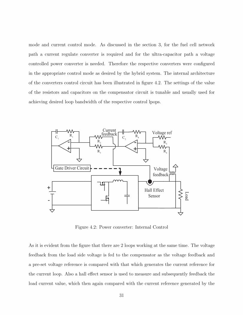
5.6 Lower Layer Operations . . . . . . . . . . . . . . . . . . . . . . . . . . . . . 63
5.7 Simulation and Results . . . . . . . . . . . . . . . . . . . . . . . . . . . . . . 64
5.8 Overall Implementation In Power System . . . . . . . . . . . . . . . . . . . . 69
CHAPTER 6: CONCLUSION . . . . . . . . . . . . . . . . . . . . . . . . . . . . . . 73
APPENDIX : INPUT TO STATE STABILITY . . . . . . . . . . . . . . . . . . . . 74
vi

LIST OF REFERENCES . . . . . . . . . . . . . . . . . . . . . . . . . . . . . . . . . 76
vii

LIST OF FIGURES
Figure 2.1:Real and reactive power flows[2] . . . . . . . . . . . . . . . . . . . . . . 7
Figure 2.2:Block Diagram of Speed droop control of generators [33] . . . . . . . . . 8
Figure 2.3:Plot of Frequency vs Active power [33] . . . . . . . . . . . . . . . . . . 9
Figure 2.4:Plot of Voltage vs Reactive power [33] . . . . . . . . . . . . . . . . . . . 11
Figure 2.5:General Structure of an inverter controlled Microgrid . . . . . . . . . . 13
Figure 2.6:General Structure of a microgrid [46] . . . . . . . . . . . . . . . . . . . 15
Figure 3.1:Block Diagram representation of SOFC System . . . . . . . . . . . . . . 18
Figure 3.2:Schematic of Hybrid SOFC System with Decentralized Controller . . . 19
Figure 3.3:Energy Conservation based Approach . . . . . . . . . . . . . . . . . . . 21
Figure 3.4:Conservation of energy with a Conservative Estimate of η2 and η2 . . . 24
Figure 3.5:Dissipation Circuit . . . . . . . . . . . . . . . . . . . . . . . . . . . . . 25
Figure 3.6:System response with a PI controller for dissipation . . . . . . . . . . . 26
Figure 3.7:Simulations with Voltage Modulation and Efficiency Estimation . . . . 28
Figure 4.1:two-quadrant Power converter topology . . . . . . . . . . . . . . . . . . 30
Figure 4.2:Power converter: Internal Control . . . . . . . . . . . . . . . . . . . . . 31
viii

Figure 4.3:Schematic of Signal Flow in K1 . . . . . . . . . . . . . . . . . . . . . . 33
Figure 4.4:Implementation of External Voltage Modulation on C2 . . . . . . . . . 34
Figure 4.5:(a) Schematic for PWM generator. (b) Discharge Circuit. (c) Gate
Driver. (d) Switching Circuit. . . . . . . . . . . . . . . . . . . . . . . . 36
Figure 4.6:Experimental Test Stand . . . . . . . . . . . . . . . . . . . . . . . . . . 36
Figure 4.7:Typical Dspace control panel during operation . . . . . . . . . . . . . . 38
Figure 4.8:Experimental Results for Dissipation Based Approach . . . . . . . . . . 39
Figure 4.9:Experimental Results for Voltage Regulation Based Approach . . . . . . 41
Figure 4.10:Power Loss patterns with Voltage Regulation and Dissipation based
framework . . . . . . . . . . . . . . . . . . . . . . . . . . . . . . . . . . 43
Figure 5.1:Two layer control structure . . . . . . . . . . . . . . . . . . . . . . . . . 49
Figure 5.2:Mapped Graph . . . . . . . . . . . . . . . . . . . . . . . . . . . . . . . 51
Figure 5.3:Decentralized Framework . . . . . . . . . . . . . . . . . . . . . . . . . . 64
Figure 5.4:Simulation Result for topology 1 . . . . . . . . . . . . . . . . . . . . . . 66
Figure 5.5:Simulation Result for topology 2 . . . . . . . . . . . . . . . . . . . . . . 67
Figure 5.6:Effect of varying topology . . . . . . . . . . . . . . . . . . . . . . . . . 68
Figure 5.7:Inverter Control Scheme . . . . . . . . . . . . . . . . . . . . . . . . . . 70
Figure 5.8:Overall system diagram Combining power system layer and control layer 72
ix

LIST OF TABLES
Table 4.1: Equipment specifications . . . . . . . . . . . . . . . . . . . . . . . . . . 37
x
CHAPTER 1: INTRODUCTION
In the rapidly changing Power grid operations, the integration of distributed generators to
the power grid has become a much debated issue. A number of groups have tried to ad-
dress this problem in significant details. Essentially, with the advent of Power Converter,
controlling the out put voltage and frequency has become an achievable target. However,
the practical application requires large number of power sources and loads to be intercon-
nected and naturally the load sharing among them becomes a challenging task. Parallel
operating sources are certainly a solution but with possibilities of power line disturbances
and intermittent nature of most of the comparatively high yield renewable sources, makes a
simpler paralleling ineffective. Naturally, separately controlling each of the inverter/sources
in a parallel connected mode was developed in [2]. With these capabilities in the power
layer of the grid, a sophisticated framework is required which will essentially determine the
reference of the output power for each distributed generators(DG). In [1, 3], the author de-
veloped some effective power management strategies to control active and reactive powers in
DGs both in autonomous and islanded mode. In [4],[5], the voltage and power angle droop
has been utilized to make the control decentralized. Some load side management schemes
were also been investigated [7], and secondary control were necessary to implement an in-
telligent control framework necessary for smarter grid operations. However all these control
strategies are more or less non-flexible as integration of renewable sources brings in a factor
of non-realibility in the system and droop methods cannot function effectively in case of
source intermittency. Also, in the islanded mode of operation an additional communication
is required for secondary control functions and power management,as described in [6]. In
addition to this, the conventional control strategies may exhibit stability issues with high
penetration of DGs as discussed in [9].
1

The control and stability of large networked system has drawn a lot of interest due to the wide
application area, and requirement of proper control for the large system stimulated interest in
distributed control in recent years. The implementation, cost and reliability of such systems
are important aspect of consideration, and naturally, the decentralized control strategies
emerges as a suitable candidate due to the size and the complexity of such systems along with
the difficulties in controlling them. A detailed description of such complex systems is given in
[71]. The core challenges are dimensionality, information structure constraints, uncertainty
and delay. Related work on decentralized stabilization of interconnected dynamical systems
appears in [69, 70]. Decentralized control on power grids as a complex large scale dynamical
system appears in [64, 65], where the authors address robust stability of large-scale power
systems. On the other hand, operating such large scale systems is also required to be fault
tolerant and reliable. To address that, the issue of cascaded tripping in power networks
can be dealt with a decentralized architecture given in [66]. In [67], a novel decentralized
fault tolerant control structure was developed using droop control. Additionally, to mitigate
cascaded failures in large power network, multi-agent based decentralized control using a
novel optimization framework can be found in [68].
Advancements in multi-agent systems and distributed control strategies along with advanced
optimization frameworks addresses the dynamics of electricity market as well as the optimal
scheduling approach as described in [7],[8], whereas some research efforts were dedicated
towards the transient stability of the system and optimal load dispatch using cooperative
control methods and game theory approach in [10],[11]. Also, some LQR based design on
synchronicity of networked system has been studied in [10] . However, these frameworks
are inherently leader-follower type, which require selection of leader agents and that brings
in the task of maintaining reliability of the leader node. However that may not always be
practically possible and cost effective.
2

Therefore a more flexible framework with each control points enjoying an equal importance
was required for stable operation of microgrid [17] both in grid connected and islanded mode
of operation, and that too in decentralized fashion. In this work, we look at a mush simpler
and scaled down version of the problem at first and try to address the decentralized control
aspect of the problem using conservation of energy principle on a small hybrid power system
consisting of a fuel cell and an ultra-capacitor. With the progress of the work, we look
for a more rigorous and scaled up version of the problem where a large number of sources
can be integrated to the grid. Here the control system itself has been treated as a set of
coupled autonomous systems. The interaction between the autonomous systems has been
made modulating so that the equilibrium point can span across a defined possibility region.
Also, efforts have been made to simultaneously reduce the amount of interaction between
the nodes and still achieve the same performance. Frequently, the system has been referred
through an equivalent graph, however the analysis has mainly been done using systems
theory. Only to demonstrate the physical variation of the system parameters and the effect
of the interconnections, a graphical portrayal of the system is presented. Linking back to
the micro grid discussion, the main objective of the work is decided to be the effective
load sharing between DGs in steady state condition, also assumption has been made on the
sufficiency of the storage/reactive elements of the power system to take care of the voltage
stability issues.
The framework directly controls the inverters connected to the grid or synchronous generators
with active/reactive power control loop which forms the power system layer, although an
effort has been made to present the work in general terms in its design phase, so that it can
be equally applied to any distributed system.
Following chapter encompasses the general structure of a power grid and existing strategies
of active and reactive power control. We will look into greater details of the application
3

of sophisticated controllers on smart grid application. Following that we will introduce the
prior works that were done on a small scale equivalent of the grid which entails conceptual
development of the controller and verification through simulation. Following that we discuss
the experimental verification of the energy conservation based framework on a laboratory
prototype. In the next chapter we introduce the novel framework for controlling the active
power based on coupled autonomous system theory followed by a complete description of
power flow controllers on a power grid and simulation results.
4

CHAPTER 2: BACKGROUND AND RELATED WORKS
Power network being the oldest and most reliable machine ever built by humans, stood
strong against the flow of time and continued to provide quality electricity. However, with
the modernization of society the demand and quality requirements of consumable electricity
has been increased significantly. To cater to the growing need of power quality and reliability,
a ’smarter grid’ is envisioned. The formal definition of smart grid is to couple the commu-
nication and cyber-physical system to the more rudimentary power network and achieve a
more developed grid system which simultaneously control the power flow depending on real
time power market scenarios, outage status, network configuration and the transient load
variations[62]. A no of sophisticated approaches were proposed for the challenging task of
the power control with so many different aspects taken into configuration. Naturally, in
the present time of modernization and pinnacle of technological advancements, no straight
forwards source-load concepts dominate the powergrid, instead, with the advent of hybrid
electrical vehicle and concept of self sustaining energy sources, such as UPS (Uninterruptible
Power Supplies) [25] prevails. Therefore, treating each control points of the network as of
same generic characteristics, and yet designing a control system that addresses all possible
control problem that may arise in different situation, is quite a challenge. Also, the growing
need for integrating renewable energy sources into the grid, comes with a challenging task of
accommodating all the inherent intermittency [26, 27] and non-reliable nature [28] of some
of these renewable and non-conventional sources. In this chapter we shall revisit some of the
existing classical approaches in existence for controlling the power flow in the network, then
we will gradually transcend to the modern approaches undertaken in order to improve the
load sharing problem.
5

2.1 Classical Active and Reactive Power Control in Power System
The control of frequencies in power grid operations are critical, and it influences the active
power control of the power grid as well as the steady state stability. Similarly the voltage
control of the network influences the reactive power control and vice versa. Tight control
of the frequency ensures the constancy of the speed of motor drives for induction and syn-
chronous motors connected to the network and it is very important for proper functioning of
the generators as they are highly dependent on the auxiliary drives used in different aspects
starting from fuel mass flow rate to feed-water and combustion of air supply. Also, motors
used in industry comes with a drives calibrated for a set power frequency, and hence proper
functioning of all industrial motors highly depends on the system frequency. The frequency
and the speed of the synchronous generator is related as
f =pn
120(2.1)
where, p is the number of pole pairs and n is the speed of the machine in r.p.s. Again, the
active power of the machine is given as
p = Teff ωm (2.2)
whre Teff is the effective applied torque at the prime mover after considering the mechanical
losses, and ωm is the mechanical speed of the rotor, which can be found from the r.p.s speed
mentioned before as,
ωm =n
2π(2.3)
6

therefore controlling the frequency, the active power can be controlled effectively. The active
power and reactive power of a network can be expressed as following [2] and [33]
P =V
ω
E
Lfsinδ (2.4)
and
Q =V 2
ωLf− V E
ωLfcosδ (2.5)
where ω is the electrical speed of the machine, P and Q are the active and reactive powers
flowing through the network, Lf is the inductive reactance or inductance of the transmission
line (which is assumed to be predominantly inductive, as it is in the practical scenario).V
and E are the voltages at the source and receiving end. A quick illustration of the system is
given in the following figure.
∂
−V
−E
−V
−E
−I
Lf
Figure 2.1: Real and reactive power flows[2]
7

2.2 Speed Droop and Active Power Management [33]
Speed droop control strategy is a very reliable method to control the frequency of the grid by
controlling the speed of the generators. In case of conventional synchronous governors[33],
the speed regulation can be represented by the following block diagram, details of which can
be found in the cited text.
mf
mf
Figure 2.2: Block Diagram of Speed droop control of generators [33]
Where a typical droop of mf has been introduced where mf is percent speed regulation or
the droop. The graphical representation of the mf has been depicted in the picture follows.
8

1.00
0
f
∆
P∆
Active power output(p.u) (P)
Frequency or speed(p.u) (r.p.m)
PfP0 P*
*
ωω
ω
ω
Figure 2.3: Plot of Frequency vs Active power [33]
Therefore, as the regulation index mf effectively describes the slope of the speed droop curve,
it is quite standard to use a speed droop curve to regulate the active power out put of the
generator.
Mathematically, the speed droop control can be represented as follows,
f∗ = f0 +mv(P∗ − P0) (2.6)
mf =ff − f0Pf − P0
(2.7)
9

In the context of microgrid operation, active power control is a very important issue, where
grid synchronization is not available in certain mode of operation (e.g islanded mode). How-
ever, the droop control method has been extensively used here for normal mode of operations,
[29, 30, 31, 32]. Electronically interfaced power sources such as inverter controlled renewable
sources were also reported to be effectively controlled using droop control method in [1, 3].
Where as control parallel inverter control for a stiff ac system using droop principles were
presented in [2, 4]. A detailed comparison of the variations of the speed droop curve and
their effectiveness on active power management are detailed in [47].
2.3 Voltage Droop and Reactive Power Management [33]
As equally important as the active power counterpart, the reactive power of a network plays
very important role of transient stability of the system. Similar to the speed droop control
in case of active power management, a voltage versus reactive power droop curve fig.(2.4) is
used for regulation of the voltage across the generator.
Mathematically, the voltage droop control can be represented as follows,
V∗ = V0 +mv(Q∗ −Q0) (2.8)
mV =Vf − V0Qf −Q0
(2.9)
where mv is the slope of the voltage droop curve.
However the generating unit provides the primary means of control however, as typically
the grid spans across huge geographical area and therefore it is unavoidable to have large
10

transmission lines joining the source to load. This additional element of the network causes
power losses over the network and the voltage at different points of the network is usually at
different volatge levels, and hence to improve the quality of power over the network, static
VAR compensators (SVC) are used[33]. Also, static shunt/series capacitors, shunt/ series
reactors are frequently used to maintain voltage in the transmission and distribution lines
[33, 54] and in [55].
1.00
V0
Vf
V∆
Q∆
Reactive power output(p.u) (Q)
Voltage(p.u) (V)
QfQ0 Q*
V*
Figure 2.4: Plot of Voltage vs Reactive power [33]
In [51], the voltage rise induced by the active power variation is shown to be controlled by ap-
propriately tuning the reative power out put at the generator terminal with out changing the
power factor too much, shown to be an improvement over the lag/lead power factor control.
However Distribution Network Operator(DNO) practices onload tap changer in distribution
11

transformer to mitigate voltage rise issues depicted in [52]. The new improvements in voltage
rise mitigation in [51] is efeective in conventional power grid, however with high penetration
of DGs and electronically interfaced power sources or inverter based distributed power gen-
eration requires more sophisticated control design. In [53], a reactive power injection based
control was described which shown to be effectively control inverter based DGs.
2.4 Voltage Source Inverters and Their Application on Microgrids
Voltage source inverters (VSIs) have been used as an essential means of power conversion for
better control and reliability purposes. Extensive discussion on the structure and working
principles of a VSI can be found in [25]. Application of VSIs in microgrid distributed
generation has been a wide spread trend because the enabling technology VSIs provide to
implement advanced control systems. In works [2, 34, 35], several different current, voltage,
active or reactive power control strategies are described for wide application areas such as
motor drives, grid applications etc. Some more advanced control techniques used in works
[36, 37] to further improve the performance of the converter. Cascaded PI control loops were
implemented in [39] in order to use VSI in a microgrid environment.
Numerous power management strategies have been developed with invertyer controlled DG
units in a microgrid, the details of which can be found in [1]-[5]. The core power management
strategy is often droop based control[1, 2, 3], however some other interesting solutions have
been suggested in [21, 29, 32, 34]. A detailed block diagram representation of a inverter
controlled DG power management can be found in the fig.(2.5).
12

Utility Grid
Load PCC
Renewable power sources, Solar, Wind etc
Energy Storage Elements, Battery,
Capacitor etc
Local Bus
Local Loads
Transmission Line
Inve
rter
Hydro power, Captive power
plant, etc
Energy Storage Elements, Battery,
Capacitor etc
Local Bus
Local Loads
Transmission Line
Inve
rter
DG1 DG2DG3 DG4
. . . . . .
Common Bus
Figure 2.5: General Structure of an inverter controlled Microgrid
The point of common coupling (PCC) signifies the coupling point of the microgrid with the
larger grid. The main utility grid supplies a portion of the total load on the grid and also
provides/receives power from each of the microgrid connected to it through the PCC. Also,
each of the DGs shown in the figure are connected to the PCC as well as to the utility grid
through inverters. Additional reactive power support has been provided by implementing
energy storage element to the DGs. Similar approaches can be found in [1, 3].
13

2.5 Distributed Generators and Impact on Microgrids
With the modernization of the power grid and more integration of the renewable energy
sources have become a preferred choice, especially since the growing concern for carbon foot-
print which is increasing with fossil fuel based power generation systems. Renewable sources
provide clean and sustainable source of energy, and naturally is preferred over the thermal
energy counterpart. However, integration of renewables poses a challenging task as often the
renewable sources are dependent on natural processes and therefore are geographically sparse
and non-flexible iin terms of its operation capability. Therefore this distributed generators,
in order to integrate to the larger grid, needs proper means of integrating devices and so-
phisticated control methodologies. A voltage source inverter(VSI) is one of the best choices
available to integrate distributed resources to the grid, However the power management be-
tween several distributed generators connected to the grid via VSCs is quite a challenge as
many researchers over the years attempted to formulate good power management strategies.
In the following subsections, a brief discussion about the architecture and control of voltage
source converters will be discussed which will be followed by a discussion on the presently
available power management strategies and their merits and demerits on the larger context
of grid operation.
14

Figure 2.6: General Structure of a microgrid [46]
Many research groups have also worked on the transient stability of the microgrid in great
details and have pointed out the influence of the distributed generation on the microgrid
[48, 49] which talks about planning tools and general conclusion on the stability issues
with high penetration of DGs into a microgrid. However problems associated with high
penetration of DGs are discussed in [50] and in [51]. As discussed previously, the voltage
control issues typically contribute to the transient stability of the grid and the active power
control ensures the demand-supply and the network quality and reliability issues. With
15

the proliferation of smart operation of microgrids with the integration of renewable energy
sources and inverter based DGs, significant research efforts were made in [1]-[11].With a
combined system of energy storage elements and the inverter controlled DGs with proper
control strategies, the smart operation can be performed in a microgrid as proposed in
[10, 11, 12, 16, 22, 57], using a cooperative control approach. Also numerous other control
strategies are proposed for the power management of a power grid or micro grid in works
[1]- [7]. However as the size of the grid increases the complexity associated with designing
the proper control framework increases as well. Multi-agent based control structure has
gained quite popularity recently [12, 58, 59]. Although cooperative and multi agent based
control of power flow brings in an exciting and new perspective to the problem, they are
often optimization based approaches[10, 11, 12, 60] and complexity of the computation is
very high which requires high end computation power and resources, and the complexity
progressively increases with the increase of the network size. Therefore this necessitates a
much simpler and easy to implement control framework that effectively addresses all the
control problem posed and requires much less computation power. With the existing pool
of resources, we look for a novel control framework to control the power flow in a microgrid.
16

CHAPTER 3: PRIOR WORK ON DECENTRALIZED POWER
MANAGEMENT OF HYBRID NETWORK
With the backgrounds and related works outlined in the previous section, we started formu-
lating the power flow control or the load sharing control problems in a multi DG microgrid.
Since a modern power system scenario has been assumed, for smart operation of the system,
every limitations of each of the component and the overall system is required to be kept in
mind.
In works [61] and in [62], the guidelines about the smart operation of a power grid is discussed.
The preserving of assets by not going beyond the absolute current or voltage or power limits
of equipment, maintaining a secondary control over each DGs so that an emergency shutdown
may be applied in the event of a failure, fault tolerant operation of power sources or catering
to any local disturbances with out affecting the larger grid operation are one of the most
important constraints to e addressed while supplying the demanded power from the utility
grid. The first steps in achieving that goal are essentially modeling a smaller part of the
microgrid along with its constraints as discussed and try to develop a control algorithm
that addresses them all while successfully supplying the demanded quality power. In an
attempt to develop small scale power system we choose a hybrid power network representing
a very small version of the larger microgrid. It consists of a power source, a solid oxide fuel
cell(SOFC) and a storage element, an Ultra-capacitor. Following discussions will describe
the structure of the system in consideration and the control algorithm developed to control
it in a decentralized manner.
17

3.1 System Description
The SOFC system considered in this work is depicted in Fig.3.1 and is identical to that
developed and discussed in [41] and [42]. Details are omitted for brevity.
catalystbed
STEAM REFORMERTUBULAR SOFC STACK
anode
cathode
Nin
Nf
No
Nair
COMBUSTOR
combustionchamber
ReformedFuel
Air Flow
Exhaust
Fuel Flowelectrolyte
Pre-heatedAir
Arrows represent heat exchange
air supply
kNoRecirculated Fuel
GAS MIXERFUEL SUPPLYSYSTEM
Nf,dDemandedFuel Flow
FSS
Figure 3.1: Block Diagram representation of SOFC System
Fig.3.2 demonstrates a schematic of the hybrid system with a decentralized control scheme.
Other approaches for building a fuel cell ultra-capacitor/battery are presented in [43, 44].
In our approach, the fuel cell and the ultra-capacitor are connected in parallel. The fuel
cell supplies power to the load through a uni-directional DC/DC converter C1. The ultra-
capacitor is connected to the load through a bi-directional DC/DC converter C2 allowing
charge and discharge. Due to their fast responses, C1 and C2 are assumed to be static energy
conversion devices, with C1 having an efficiency of η1 and C2 having discharge and charge
efficiencies of η2 and η2 respectively [42]. We also assume that η2,min ≤ η2, η2 ≤ η2,max.
18

DC/DCConv.(η1)
Fuel Cell System
K1
Load
Vfc , ifcC1
VL , iL
Nf,d. Nf
.ifc
DC/DCConv.
(η2, η2)Storage DeviceUltra-capacitor
C2
K2
Vuc , iuc VL , io
Figure 3.2: Schematic of Hybrid SOFC System with Decentralized Controller
From the schematic in Fig.3.2, since the fuel cell and the ultra-capacitor are connected in
parallel, the following is true at all times:
VLiL = η1Vfcifc +
[η2 + η2
2+η2 − η2
2sgn(iuc)
]Vuciuc, (3.1)
To control both the voltage across and current through the load, we apply current mode
controllers on C1 and voltage mode controllers on C2 to maintain a constant VL across load.
Note: Since there is a reversal of power flow direction during charge and discharge of the
ultra-capacitor, for discharge, η2 is bounded by, 0 < η2 < 1 while for charging, η2 is bounded
by, η2 > 1. This can be explained intuitively if the power input-output relation of C2 is
considered.
19

3.2 Control Objectives
Referring to Fig.3.2, the control objectives are:
1. Power demand: The net power demand VLiL should be met by the hybrid power
system at every instant.
2. Fuel utilization: The target fuel utilization at steady state will be Uss = 0.8 while
the deviations from Uss during transients should be minimized [41, 42].
3. SOC (State-Of-Charge): Control scheme is designed to maintain the SOC of the
ultra-capacitor at the target value of St.
4. Decentralized controllers: Design K1 and K2 (referring to Fig.3.2) with no mutual
information sharing.
To realize a decentralized control, we impose the following restrictions on K1 and K2. Con-
troller K1 can use measurements of Vfc, VL, iL and η1. However, it does not have measure-
ments of iuc, Vuc or η2. It commands C1 to draw ifc. Controller K2 measures Vuc, iuc, but
does not have measurements of ifc, Vfc, VL, iL or η1. K2 commands C2 to maintain a desired
VL.
3.3 Decentralized Power Management Using Energy Conservation
3.3.1 Approach
This work applies conservation of energy to develop decentralized control of the hybrid
system in Fig.3.2. Conceptually, the approach is illustrated in Fig. 3.3.
20

Time (s)190 200 210 230 250
300
400
500
600
Pow
er (w
)Power Demand (VLiL)
Power Supplied (η1Vfcifc)A2
A1
Figure 3.3: Energy Conservation based Approach
The figure shows a step change in power demand and the corresponding load-following re-
sponse of the source (fuel cell). The area A1 represents the energy supplied by the storage
device (ultra-capacitor in this case) to make up for the fuel cell’s deficiency for load following.
Therefore, if the area A2, which represents the extra energy supplied by the source, is same
as A1, that ideally charge the capacitor to its original SOC. Extending this idea, we note
that if∑
iA1,i =∑
k A2,k, i.e. if
limt→∞
EA = limt→∞
(∑i
A1,i −∑k
A2,k
)→ 0 (3.2)
then the storage element will maintain its original energy level. Ideally, the above condition
can be satisfied by K1 without any information about the capacitor by just ensuring
limt→∞
∫ t
0
4P dt = 0, 4P , (VLiL − η1Vfcifc) (3.3)
In the presence of losses in C2 with discharge and charge efficiencies η2 and η2 respectively,
21

Eq.(3.2) is modified to
limt→∞
EA = limt→∞
(∑i
A1,i
η2−∑k
A2,k
η2
)→ 0. (3.4)
If we assume η2 and η2 to be known then, using 4P as defined in Eq.(3.3), Eq.(3.4) is
satisfied by K1 by ensuring
limt→∞
Ie= 0, Ie,∫ t
0
[η−12 + η−12
2+η−12 − η−12
2sgn(4P )
]4Pdt (3.5)
To demonstrate that conservation of energy approach can be used in principle to design
decentralized control, we consider a simplified scenario. Assuming that in addition to the
local information mentioned in Assumption 2, controller K1 has exact knowledge of η2 and
η2. Next, in designing K1, we recall that the commanded ifc must be based on the actual fuel
flow Nf for transient control of U , as detailed in [41]. Also, Nf is driven by the demanded
fuel Nf,d, which in turn is determined from ifc,d. Thus, the command ifc to C1 can be
determined as:
Nf,d =ifc,dNcell4nFUss
β ⇒ ifc =4nFUssNf
Ncellβ, (3.6)
where β = [1− (1− Uss) k]. From Eq.(3.6) it can be noted that designing K1 reduces to
the design of the reference ifc,d. The design of ifc,d is based on the following observation:
In load-following mode, the fuel cell provides the entire power demand at steady-state and
uses transient perturbations in power to regulate the ultra-capacitor SOC. With this goal,
and incorporating the approach outlined in section 3.3.1, we formulate ifc,d as:
ifc,d =VLiLη1Vfc
+ kiIe, ki > 0 (3.7)
where Ie is defined in Eq.(3.5). This design is implemented and simulation results are
22

summarized in Fig.3.4. The parameter values chosen are
C = 25F, η1 = 0.8, η2 = η2 = 0.8, ki = 0.01 (3.8)
The power demand VLiL is subjected to step changes. We note that K2 simply maintains the
constant voltage VL across the load. However, η2 and η2 will be unknown to K1. Therefore,
we need to build a robust control around this principle to handle the uncertainty in a
decentralized manner. The next section will demonstrate the validity of the main principle.
3.3.2 Robust Performance Through Dissipation
3.3.2.1 Design of K1 Using a Lower Bound on η2 and η2
Considering a more realistic case where K1 has no information of η2 and η2 but only knows
a lower bound η2,min ≤ η2, η2. Accordingly, in Eq.(3.7), instead of using Ie from Eq.(3.5), a
conservative Ie is used:
Ie ,∫ t
0
[η−12,min + η2,min
2+η−12,min − η2,min
2sgn(4P )
]4Pdt (3.9)
It can be observed that Eqs.(3.6), (3.7) and (3.9) together generate a feedback loop. This is
because the FSS dynamics, considered nonlinear and unknown, relates ifc to ifc,d through a
general form
difcdt
= f (ifc, ifc,d) , such that limt→∞
ifc = ifc,d. (3.10)
It is evident from Eqs.(3.7) and (3.9) that for a step change in iL, limt→∞∆P = 0. Moreover,
since ∆P = iLVL−η1Vfcifc, hence from Eqs.(3.10), limt→∞ ifc,d = ifc = iLVL/η1Vfc and that
limt→∞ Ie = 0. We omit formal stability proof for brevity.
23

Simulation results with Ie calculated using Eq.(3.9) are shown in Fig.3.4. The parameter
values chosen were same as in Eq.(3.8). Additionally, η2,min = 0.7 was chosen.
100 300 500
0.75
0.8
0.85
0.9
100 300 500200
400
600
800SO
C
Pow
er (W
)
Time (s) Time (s)
(a) (b)
VLiL
η1Vfcifc
Figure 3.4: Conservation of energy with a Conservative Estimate of η2 and η2
The formulation of Ie according to Eq.(3.9) is conservative since it always overestimates and
underestimates the energies from and to the capacitor respectively. The conservative nature
of this approach can be inferred from Fig.3.4(a) where the SOC builds up with changes in
power demand. The power demanded and power supplied are plotted together in Fig.3.4(b).
Since the ultracapacitor is of finite capacity, one must regulate the SOC. To address this in
a decentralized manner we design dissipation based controller K2.
3.3.2.2 Dissipation Based Design of K2
In this approach, the ultra-capacitor’s SOC is regulated via dissipation through a variable
resistance. We choose to add a resistance in parallel with capacitor which is shown in Fig.3.5.
Energy dissipation is controlled by K2 by actuating a pulse-width-modulated switch S1,
shown in Fig.3.5. Since the SOC is a local information for K2, charge management is done
locally without any information about the fuel cell from K1.
24

iRC R
iuc
Figure 3.5: Dissipation Circuit
The circuit equation corresponding to Fig.3.5 is:
CVuc = −(iuc + iR), Vuc = − 1
C(iuc + VucσR) (3.11)
where σR is the effective conductance that can be varied by changing the duty cycle of S1.
We treat σR as a control input and use the following control law to stabilize the equilibrium
Vuc = Vuc,d
σR =kp,ucVuc
(Vuc−Vuc,d)+ki,ucVuc
∫ t
0
(Vuc−Vuc,d) dt,
σR = 0, if σR = σR,max and Vuc > Vuc,d
σR = σR = 0, if Vuc ≤ Vuc,d
(3.12)
where Vuc,d is such that Vuc,d/Vuc,max = St, the target SOC. The efficacy of this controller is
shown through the simulation results in Fig.3.6. The manner in which the resistanceR is used
in the PI control is evident from Fig.3.6(b). For this simulation, St = 0.8 and Vuc,max ≈ 16V,
and hence Vuc,d = 13V. Also, kp,uc = 0.08 and ki,uc = 0.0016. We assume R = 25Ω, and that
σR varies linearly with from duty cycle = 0 ⇒ σR = 0, to duty cycle = 1 ⇒ σR = 0.04.
25

(a)
200 300 400 5000.7
0.74
0.78
0.82
0.86
Time (s)
SOC
(a
200 300 400 500
0
0.01
0.02
0.03
0.04
σ R (O
hm-1
)
(b)
Time (s)
Time (s)500400300200100
200
400
600
800
Pow
er (W
)
(c)
Figure 3.6: System response with a PI controller for dissipation
In contrast to Fig.3.4(a) where the SOC control was not implemented in K2, the SOC
converges to 0.8 with the control law of Eq.(3.12).
Note that in Eq.(3.12), we did not incorporate iuc in the feedback although it is a local
information. The reason is that we want σR to respond only to gradual (i.e. low frequency)
changes in Vuc and not respond to high frequency components of Vuc or perturbations in iuc.
The current iuc can be considered as a disturbance in Eq.(3.11). In load-following mode, iuc
would be close to zero and hence the noise-to-signal ratio of its measurement is expected to
be high, especially when load variations are gradual. Since the change in SOC is expected
to be a gradual process, we want σR to respond only to the low frequency component of Vuc.
It is expected that the frequency content Ωiuc of iuc to consist of that of iL and that of ifc.
This is evident from Eq.(3.1). Considering a controller D(s) connected in series to the plant
26

G(s) = −1/(Cs) and a standard negative feedback loop, one can write
E(s) =1
1 + L(s)Vuc,d(s) +
G(s)
1 + L(s)iuc(s), E(s) = Vuc,d(s)− Vuc(s), L(s) = D(s)G(s)
(3.13)
where, the control input is iR = VucσR. Since Vuc,d is a constant, reference tracking and dis-
turbance rejection can be simultaneously achieved by the PI controller proposed in Eq.(3.12),
which translates into D(s) = (kp,uc + ki,uc/s) in frequency domain. With this configuration,
the loop gain L(s) is high at low frequencies and low at high frequencies. Moreover, the
zero at (−ki,uc/kp,uc) can be tuned to obtain a desired high frequency roll off. Furthermore,
attenuation of iuc is achieved at low frequencies due to |L(jω)| |G(jω)|, and at high
frequencies due to |G(jω)| → 0.
3.3.3 Robustness through voltage modulation
Using dissipation based approach a fixed amount of energy is generally lost every time a load
perturbation appears. The idea in the voltage regulation method is to minimize this loss.
Evidently, energy loss would be prevented if the fuel cell controller K1 has accurate knowledge
of η2 and η2. Hence, the objective of this design is to develop a mechanism by which K1 can
learn the aforementioned efficiencies without direct sensing or communication with K2. To
this end, we propose the following approach. As mentioned in section 3.8, K2 can manipulate
VL. Therefore K2 can manipulate VL based on the SOC of the ultra-capacitor. As the SOC
deviates from the target St, VL can be varied gradually by K2. Not only will it regulate Vuc,
but since VL is a global variable, the fuel cell can simultaneously use VL to improve its lower
bound η2,min. The process, if designed properly, will cause η2,min to increase, and eventually
settle close to the actual efficiency η2. This will diminish overcharging of the ultra-capacitor
with progress of time.
27

Voltage fluctuation is undesirable in power networks. Therefore, the aforementioned modu-
lation method, even though is capable of inducing the fuel cell to improve its η2,min estimate,
must be designed in a way such that voltage fluctuations are low and they diminish as the
estimate of η2,min improves. We propose VL to be modulated by K2 using an integral action
VL = VL,nom + ki,v2
∫ t
0
(Vuc − Vuc,d) dt, (3.14)
where VL,nom is the nominal load voltage. When Vuc is sufficiently close to Vuc,d, the integrator
resets VL to VL,nom. On the other hand, an integrator is used in K1 which is similar to
Eq.(3.14) to utilize the voltage deviations from VL,nom for efficiency estimation.
η2,min(t) = η2,min(0) + ki,v1
∫ t
0
(VL − VL,nom) dt (3.15)
Since η2,min(0) is a lower bound Simulation results are depicted in Fig.3.7. In the simulation,
pulsed changes in power demand were applied every 200s. Parameter values were ki,v1 =
0.0005, ki,v2 = 0.005, η2 = η2 = 0.8, and VL,nom = 24V.
0.7
0.74
0.78
Estim
ated
Eff
icie
ncy
(η2)
0 2000 4000 6000
0.74
0.78
0.82
0.86
0.9
Time (s)
SOC
(a)
24
24.1
24.2
VL
(V)
0 2000 4000 6000Time (s)
(b)
0 2000 4000 6000Time (s)
(c)
0.72
0.76
0.8
Figure 3.7: Simulations with Voltage Modulation and Efficiency Estimation
From Fig.3.7(a), it is clear K2 is able to maintain the SOC through voltage modulation.
28

Further, Fig.3.7(b) shows that voltage fluctuations reduce over time. This is primarily due
to better estimation of η2,min by K1 over time. The estimation is depicted in Fig.3.7(c).
The saw-tooth type of response as shown in Fig.3.7(b) is due to integrator resets. Another
observation is that during higher SOC/voltage fluctuations toward the beginning, efficiency
adaptation was faster, and it decreased with time. The estimation process therefore requires
not only the voltage modulation but also requires persistent perturbations in the power
demand.
29

CHAPTER 4: DETAILS OF PRACTICAL IMPLEMENTATION
4.1 Power Converter topologies
The power converters that were used for the construction of the hybrid power systems were
essentially two-quadrant half-bridge converter, and as the name suggests, bidirectional power
flow is allowed through the converter. The switches that were used are bidirectional in
nature therefore they allow current flow both from drain to source and source to drain. The
construction of the converter is shown in the fig. (4.1).
Load
Filter
Filter
Gate signals
Source
L
C
L
C
MO
SFET
s
Figure 4.1: two-quadrant Power converter topology
However, according to standard cascaded PI control scheme, the bandwidth of the current
compensator and voltage compensator are usually kept one order of magnitude higher/lower
than the other one. For our case, provisions were made to switch between the voltage control
30
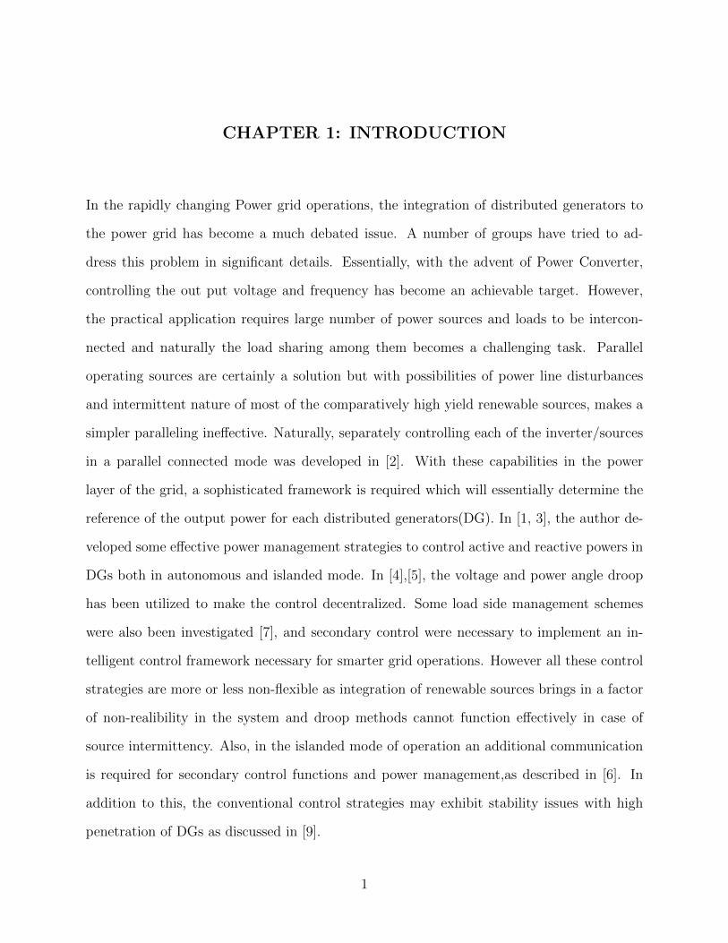
mode and current control mode. As discussed in the section 3, for the fuel cell network
path a current regulate converter is required and for the ultra-capacitor path a voltage
controlled power converter is needed. Therefore the respective converters were configured
in the appropriate control mode as desired by the hybrid system. The internal architecture
of the converters control circuit has been illustrated in figure 4.2. The settings of the value
of the resistors and capacitors on the compensator circuit is tunable and usually used for
achieving desired loop bandwidth of the respective control lpops.
Current Voltage ref
Gate Driver Circuit Voltagefeedback
+
-Hall Effect
Sensor
Load
+-
+-R1
R3
R2
R4
R5
R6
C2C1
feedback
Figure 4.2: Power converter: Internal Control
As it is evident from the figure that there are 2 loops working at the same time. The voltage
feedback from the load side voltage is fed to the compensator as the voltage feedback and
a pre-set voltage reference is compared with that which generates the current reference for
the current loop. Also a hall effect sensor is used to measure and subsequently feedback the
load current value, which then again compared with the current reference generated by the
31

voltage loop and finally this determines the gate pulse width in the gate driver circuit block.
Now, the resistance and capacitance sets of the each op-amp decides the cutoff frequency
and bandwidth of each compensator. Therefore regulating these values R1, R2, R3, C1 and
R4, R5, R6, C2 we can achieve a difference of atleast one order of magnitude difference in
the bandwidth of each compensator in order for both the loops to work simultaneously. As
shown in the fig.(4.2), both voltage and current feedback has been taken from the out put
through voltage and current sensors respectively and fed back to the comparator embedded
inside the converter to compare the desired and actual value of both the current and voltage.
Therefore both the error signals were compensated through PI regulators.
However, in our application only single loop control appeared to be the requirement and
provision has been made in the power converter so as to switch off any loop and use the
other loop independently. In the event of this operation, any of the single loop, voltage or
current when activated, will determine the required gate pulse width and generate according
gate pulses. Therefore according to system requirements appropriate control loops were
chosen and other loop has been put off.
4.2 Control of Unidirectional Converter C1
As mentioned in section 3.1, and also evident from the development in sections 3.3, and
3.3.2.1, the DC/DC converter C1 (see Fig.3.2) will be controlled in current control mode. To
apply our theory directly, K1 must command C1 to deliver ifc. However, referring to Fig.3.2,
the converter C1 in our setup allows us to command io directly and not ifc. The DC-DC
converter has an in-built controller which takes a sensed feedback of io flowing through a
hall-effect sensor inside the converter, and using a PI-controller, makes io tend towards a
commanded value io,c set by the user. To control ifc through C1, we propose the following
32

feed-forward and feedback combination:
io = io,c =η1Vfcifc,cal
VL+ kp,1efc + ki,1
∫ t
0
efcdt, efc , ifc,cal − ifc (4.1)
where η1 is a constant estimated efficiency of C1, ifc is the measured fuel cell current,
and ifc,cal is the target fuel cell current calculated using Eqs.(3.6) and (3.7), as ifc,cal =
4nFUssNf/(Ncellβ). The internal controller in C1 generates fast response, on the order of
micro-seconds. Hence we assume io = io,c in Eq.(4.1). The feed-forward term (η1Vfcifc,cal/VL)
in Eq.(4.1) comes from the power balance at the input and output terminal of the converter
C1. The sequence of signal flow is explained through the schematic in Fig.4.3.
iL Eq.(6)ifc,dEq.(7)
Nf,d Nfifc,cal
Eq.(4.1)ifc
Eq.(6)
io,cC1 io
FSSdynamics
Figure 4.3: Schematic of Signal Flow in K1
To prove that the above approach will lead to convergence of ifc to ifc,cal, we assume that
the feed-forward term is constant during the correction interval, which is reasonable if kp,1
and ki,1 are assigned relatively high values. Referring to Fig.4.3 and Eq.(4.1), we then have
diodt
=η1VfcVL
difcdt
= kp,1efc + ki,1efc ⇒(kp,1 +
η1VfcVL
)efc + ki,1efc = 0 (4.2)
In conclusion, Eq.(4.2) guarantees that limt→∞ efc → 0, provided the inequalities kp,1 >
−η1VfcVL
and ki,1 > 0 are satisfied.
33

4.3 Bidirectional Converter Control
The bidirectional converter C2 is operated in voltage control mode. The primary purpose of
this converter is to maintain a constant voltage across the load at all times. The converter
has been set to maintain VL = 23V across the load for the dissipation based method. The
choice of this value for VL is driven by the limiting output voltage of C2, which is 23.3V.
+- Compensator
C2 Internal Control
Duty RatioFor Load side
control
Voltage Feedback
+5 Volt
iv ovRef VoltageOutputVoltage
Empirical Look-up table
Voltage RegulationCommand
C2
+
-
+
-
Fixed Load voltage scheme Regulating Load voltage scheme
µ
io vvµ−
=1
1
Analog outIn
tern
al (f
ixed
) vol
tage
con
trol
External voltage regulation
Figure 4.4: Implementation of External Voltage Modulation on C2
4.4 η1 Measurement
In calculating ifc,d in Eq.(3.7), it is assumed that the measurement of η1 is available to K1,
since it is a local variable. In our experimental setup it is measured by implementing the
power balance equation for C1 to generate a coarse measurement η1,m, followed by a first
order filter of time constant τ for smoothening
η1,m =VLioVfcifc
, ˙η1 = (1/τ) (η1,m − η1) (4.3)
34

4.5 PWM Switching Circuit
The approach that was taken in Chapter 3, in equation 3.12 was essentially to dissipate excess
energy by varying the resistance or conductance of the dissipator. However, in practice we
keep the resistance constant and change the average voltage appearing across it, therefore
the same effect can be achieved here with a little modification in the theory proposed in
chapter 3. Controller K2 manipulates the duty ratio µ to change the dissipation rate as
follows:
µ(t) =kp,ucVuc
(Vuc−Vuc,d)+ki,ucVuc
∫ t
0
(Vuc−Vuc,d) dt,
µ = 0, if µ = 1 and Vuc > Vuc,d
µ = µ = 0, if Vuc ≤ Vuc,d
, σR = µσR,max
(4.4)
The average voltage appearing across the dissipating resistor, effectively determines the iR.
The relation between the duty ratio µ(t) and iR can be formulated as:
1
T
∫ T
0
VucdR(t)dt = iRR (4.5)
where 1/T is the switching frequency of the PWM. The PWM circuit will be switched off as
soon as the equilibrium Vuc = Vuc,d is established. The hardware consists of a simple solid-
state switch which drives the gate of a power MOSFET of appropriate rating whenever the
ultra-capacitor voltage surpasses a certain threshold voltage. The voltage reference is set to
12.2V above which the PWM circuit activates. Moreover, the rate of discharge is controlled
by the pulse-width of the PWM signal that is realized by driving the gate of the MOSFET.
The gate driver circuit consists of UCC27322 gate driver IC which can produce 9A peak
current at the Miller Plateau region of the MOSFET [45]. Schematics and hardware of the
PWM circuit are shown in Fig.4.5.
35

Dissipating Resistor
Control SignalsGate Driver IC,UCC27322
MOSFET IRF740
PWM Power Source (d)
Figure 4.5: (a) Schematic for PWM generator. (b) Discharge Circuit. (c) Gate Driver. (d)
Switching Circuit.
Figure 4.6: Experimental Test Stand
The hardware setup is illustrated in the fig.(4.6). The specifications of the equipment used
here in the figure are tabulated in the table.(4.1).The hardware in the loop (HIL) approach
36

was implemented in the real time processor Dspace.
Table 4.1: Equipment specifications
Item Specification(Voltage) Specification(Current) Other Specification Make
dSpace i/p:120V AC - - dSpace1103
Power Supply 110V AC/DC o/p:50A Programmable Ametek SGA100/50
Electronic Load i/p:120V AC 0-120A, 0-1.8KW, 0-1790ohm Programmable Sorenson SLH
Ultracapacitor 16.2V DC - 250F Boostcap, BMOD0250 P16
Unidirectional Converter 44-50V DC 40A Programmable Zahn Elect. DC-5050F-SU
Bidirectional Converter 44-50V DC 40A Programmable Zahn Elect. DC-5050F-SU
Current Sensors - 1-100A Bandwidth 100KHz Fluke-80i-110S
Voltage Sensors 0-1KV 10mA Resistance divider -
The mathematical model of the SOFC and its characteristics were embedded in the Dspace,
and the response of the theoretical model was sent in real time to a programmable DC
power supply given in table.4.1. Hence, the Dspace and the programmable DC power supply
collectively represented the SOFC system, however limited by the accuracy of the theoretical
model. Along with the HIL, both the controllers K1 and K2 mentioned in section.3.3.2.1
and section.3.3.2.2 and later on in section.3.3.3 were implemented in the Dspace processor.
In addition to the implementation, another important function was served by the Dspace
was to monitor the signals and values of different parameters of the system at all times, to
ensure smooth operation of the system. The Control panel platform of the Dspace was used
for all monitoring and parameter tuning in the middle of the operation. The figure below
illustrates a typical control panel of Dspace platform during operation.
37

Figure 4.7: Typical Dspace control panel during operation
4.6 Experimental Results
The detailed experimental validation and the illustration of system behavior with a step load
change has been demonstrated here in this section. Both dissipation and voltage regulation
based approaches are discussed along with the experimental data obtained for both of then
followed by a comparative study of the effect of both the approaches on system efficiency.
The load resistance was given a periodic step change, usually from 1.2Ω to 2.4Ω, to test the
system and controller response to a step change in the load and its performance, when this
step change is persistent.
4.6.1 Experimental Validation of Dissipative Method
The decentralized approach with dissipation based SOC control, discussed in sections 3.3
and 3.3.2 is tested on the experimental setup and results are shown in Fig.4.8. As shown
in Fig.4.8(a), a repetitive step load change from 10A level to 20A level is implemented.
Fig.4.8(d) confirms transient fuel utilization control, with only ≈ ±2% deviation about the
38

target Uss = 80%. Fig.4.8(b) and (e) are self-explanatory, representing fuel cell current and
voltages. Fig.4.8(f) compares Vuc with (blue) and without (red) dissipation. For the test, we
set St = 0.75, which corresponds to Vuc,d ≈ 12.2V. The conservative nature of K1 is clear,
since it gradually overcharges the capacitor in the absence of dissipation (in K2). With
controlled dissipation the issue is addressed.
(b)
76
84(d)
30 ifc (A)(a)
iL (A)
35
(e)50
Vfc (V)
%
12.5
(f)
Vuc w/o control (V)Vuc with dissipation (V)
(c)iuc (A)
(g)
time (s)
(-)ve indicates discharge
A1
A2
Figure 4.8: Experimental Results for Dissipation Based Approach
In the experiment, the controller parameters are chosen as follows: For K1, ki = 0.01 in
Eq.(3.7) and kp,1 = ki,1 = 0.01, η1 = 0.85, in Eq.(4.1) and for K2, kp,uc = 0, ki,uc = 20
in Eq.(4.4). In Fig.4.8(c), iuc is plotted. As expected, iuc goes to zero at steady-state,
indicating that indeed the fuel cell supplies the entire power demand at steady-state. The
slow response of the FC to the load changes, along with the capacitor’s contribution to make
up for FC’s deficiency during load transients is visible in Fig.4.8(g). In this plot, also observe
that A1 < A2. This is due to losses in C2 which translates to Eq.(3.4) for conserving the
capacitor’s energy.
39

4.6.2 Experimental Validation of Voltage Modulation
Voltage modulation capability was facilitated in the converter C2 with minor changes to its
internal circuitry. Hardware limitations of C2 limit the maximum VL,nom to ≈ 23.3V. Hence,
to allow voltage modulation VL,nom = 22V is chosen in Eq.(3.14). The modifications to C2
to implement voltage modulation are shown in Fig.4.4.
Two integrators were used at the FC side (i.e. K1) to utilize the load deviations from 22V
for efficiency estimation, to account for the different discharging and charging efficiencies,
namely η2 and η2 respectively.
η2(t) = η2(t0) + ki,v11∫ t0
(VL − 22) dt, ˙η2 = 0, when discharging
ˆη2(t) = ˆη2(t0) + ki,v12∫ t0
(VL − 22) dt, ˙η2 = 0, when charging(4.6)
In the experiment, the following parameter values were chosen, ki,v2 = 0.1, ki,v11 = 0.001,
ki,v12 = 0.002 and η2(t0) = ˆη2(t0) = 0.7. The experimental results are shown in Fig.4.9.
40

0 1000 2000 3000
22
22.5
23
1600 1800 2000
12.5
13
1600 1800 2000−20
0
20
1600 1800 2000
10
20
0 1000 2000 300010
20
1600 1800 2000200
400
30002000100000.75
0.85
0.95
1.05
η2η2
iL (A)
VL (V)
21.5
Vuc (V)
time (s)
time (s)
iuc (A)
time (s)12
time (s)
ifc (A)
time (s) time (s)
η1Vfcifc (W) VLiL (W)
0
time (s)
(a)
(b)
(c) (d)
(e) (f)
(g)^
^
Figure 4.9: Experimental Results for Voltage Regulation Based Approach
The power draw was pulsed at regular interval, as shown in Fig.4.9(a). Figure 4.9(b) is
the main result of the experiment, showing that load voltage fluctuations imposed by K2
diminished over time starting from ∼ 0.5V to < 0.05V . This is because with progressive
improvement of the efficiency estimates, the net capacitor overcharge over individual power
pulses reduce. The corresponding variations in Vuc, iuc and ifc are depicted in Figs.4.9(c), (d)
and (e) respectively. The load power and fuel cell delivered power are plotted in Fig.4.9(f).
The figure illustrates how K1 modulates the fuel cell power to attain energy conservation
41

in the ultra-capacitor. The estimates η2 and ˆη2 are shown in Fig.4.9(g). The estimates of
discharge and charge efficiencies settle at η2 ≈ 0.84 and ˆη2 ≈ 1.02 respectively. This, in
particular ˆη2 ≈ 1.02 is expected since it represents the charge efficiency. As mentioned in
section.3.1 and section.3.2, the charge efficiency is expected to be greater than 1 since the
energy supplied for charging the ultracapacitor will be higher than the change in the stored
energy due to losses.
4.7 System Loss Comparison
Although both the approaches described above performs satisfactorily on the task of meeting
the control objectives described in section 3.2, they have certain advantages and disadvan-
tages which makes each approach more applicable in different perspectives. The voltage
regulation based approach progressively reduces energy losses; yet it relies on persistent ex-
citation of the load to improve its efficiency estimates. On the other hand, the dissipation
based approach results in uniform energy loss, but it does not require perturbations on the
network. The energy losses with each approach were compared and plotted in Fig.4.10. Each
data point represents an average power loss over an interval, calculated as
Wloss,i =1
ti − ti,0
∫ ti
ti,0
(VLiL − Vfcifc) dt (4.7)
for both approaches. In Eq.(4.7), ∆ti = ti − ti,0 represents the ith interval ending at ti and
starting at ti,0. Each interval is roughly the same, around 100s, consisting of one step-up and
one step-down in iL. The final instants ti were not all equally spaced in time. For example,
(t5 − t4) and (t7 − t6) are longer than the others. It can be observed from the plot that
with voltage regulation, the losses decay over time whereas it is uniform for the dissipation
based approach. The overall magnitudes are not considerably different. This is because
42

the changes in capacitor voltage due to overcharging (and hence the required dissipation)
were low in our experiments, owing to a high capacity of 250F and comparatively lower
power levels, see Fig.4.8(f). It is expected that with lower capacity storage the advantages
of voltage regulation will be more prominent.
0
30
60
15
45
75
Aver
age
Loss
(W)
t1 t2 t3 t4 t5 t6 t7 t8 t9time (s)
Voltage Regulation
Dissipation
Figure 4.10: Power Loss patterns with Voltage Regulation and Dissipation based framework
However, although these verified data of the proposed decentralized scheme proves the effec-
tiveness of the approach, it transpires that applicability of this approach to a highly scaled
scenario is not a simple task. In fact, keeping this same approach and incorporating a large
no of primary power sources in place of one single SOFC cell will make the decentralized
design more challenging since all the estimation process described in section 3.3.3 are now
required to be done separately for each of the sources and naturally that makes the problem
highly complicated. Therefore, we needed a much simplistic and elegant approach to tackle
more real life problem i.e microgrid. A concise description of the microgrid is given in the
chapter-2. Moreover, in addition of more primary power sources, the load sharing between
them in steady state is still not addressed with the present approach. For example, an equal
load sharing between two SOFCs may be proposed on top of the existing framework, but
43

there is no provision has been made so that one SOFC will increase its production when
the other SOFC is limited in production due to its internal constraints, in a decentralized
manner. Therefore existing approach is apparently limited to small scale hybrid systems
only. Therefore, there is a need for a much simpler control framework which employs the
decentralized mode of operation and can be applied to large systems. Additionally, the new
framework should be able to meet all the internal constraints posed by the controlled agents,
i.e. power sources and also conforms to the power demand-supply condition. Following
chapter will describe a newly proposed approach to effective deal with highly scaled version
of the present problem.
4.8 Fault Tolerance Provisions in Decentralized Framework
As previously described in the section.1, an illustration of the fault tolerant attributes of the
decentralized controller for the hybrid system is provided here. Referring to the previous
works [41], the fuel cell current demand, ifc,d determines the fuel demand for the SOFC
which is described by the following equation.
Nf,d =ifc,dNcell4nFUss
[1− (1− Uss)k] (4.8)
where
ifc,d =VLiLη1Vfc
+ g(Es) + δ1 (4.9)
where, Es = S − St, S=SOC of the ultra capacitor and St= target SOC of the ultra capac-
itor. However in this paper, with a decentralized approach the demanded fuel cell current
expression is as follows.
ifc,d =VLiLη1Vfc
+ kiIe, ki > 0 (4.10)
44

Therefore it is clear from the above two equation that, in centralized case, the SOFC con-
troller depends on the value of the SOC of the ultra-capacitor whereas the decentralized
controller is independent of the SOC. Therefore, in the event of a fault in the ultra-capacitor,
its SOC will be perturbed. In a centralized control this will affect the SOFC fuel flow rate
and possibly the fuel cell controllers will malfunction as well, where as the decentralized con-
troller, being invariant to the SOC of ultra-capacitor, will will ensure ∆P = VLiL− η1Vfcifc,
even under such a fault. However depending upon the nature of the fault, for certain faults
such as the one mentioned here, the advantage may be clear. But for others, a secondary
protection maybe necessary for both centralized and decentralized approaches.
45

CHAPTER 5: COUPLED DYNAMICAL SYSTEM APPROACH
Transitioning from the previous approach of decentralized control of multi DG microgrid
systems, in this newly developed approach , we consider a large number of control nodes
which represent each power sources. For a strategic load scheduling, we can incorporate
loads in the set of control nodes as well. The external utility grid is also considered as a
control node, however since the microgrid is much smaller and weaker than the utility grid,
usually the external grid node is not controlled instead, it acts as an autonomous node. The
load node is considered as the input node to the system, through which the load command is
applied to the microgrid. The usual structure of a power network may often be simplified to
a collection of local loads and a set of global loads which is supplied by all the power sources
in the microgrid, which is represented by the load node L. The effect of local loads have
been ignored as the main emphasis of this work, is to demonstrate decentralized control of
multi DG system in a microgrid, therefore, the effective global load sharing among the power
sources are sufficient to prove the effectiveness of the framework. The entire cyberphysical
layer of the microgrid is mapped as a mathematical graph and all the analysis and design of
the framework has been progressed from there.
The cyberphical layer consists of the control and communication activities of a microgrid.
This encompasses the control signal sent to each power source and the circuit protection
elements in a microgrid, the communication topology between all the system elements and
their interconnection, the processing of each signal from the measuring devices, the operators
who decides the power sharing, the dynamic pricing, billing and all commercial activity, and
so on. The framework that we want to achieve will significantly reduce the efforts in control
room operations and manual tuning of power flow commands. The main objective of this
framework is to control the transient active power flow and satisfy all the requirements of
46

smart operation of a microgrid as discussed before.
To simplify our analysis and design, we divide the operation of the cyberphysical layer into
three distinct categories;
• Electricity Market, pricing, availability and economic dispatch calculation.
• Implementing dispatch commands through inverter controlled DGs.
• Measurements and estimations.
However, in conventional utility grid system, the economic dispatch calculations are done
by distribution network operators (DNO) and it obtains a specific power output figure for
each generator. In the following framework, these calculations of economic dispatch along
with the local disturbances, system limitation(e.g. current, voltage, thermal limits etc) and
manual override provisions are classified as the lower layer operation.
However, the market dependent load flow variations are slow process and our main objec-
tive in this work is to address the transient stability and transient load sharing problems
as discussed in the chapters-1 and 2. The conventional droop control methods and other
optimization based approaches have their own limitations. Therefore, we look for a novel
decentralized approach in active power sharing among a large number of power sources con-
nected to the microgrid and ensure smart operation. The decentralized approach is seen as
the limited ability of a node or agent to interact with others. The dynamics of the controller
itself has been defined as the upper layer operations. Therefore, in summary, any change
in existing configuration of the load shares, any disturbance or manual intervention can be
brought in through lower layer operation. While lower layer operation is non-functional, the
upper layer and its current structure and configuration will dictate the share of loads among
47

the generators. This way a very flexible control structure can be realized which follows all
the control objectives but when needed to be steered to a certain direction by users choice,
there is no restriction to commit a manual steering operation.
5.1 System Description
The system structure under discussion is made into two different layers to separate out the
functionality and hierarchy. The controller in the lower layer is primitive in nature and the
main function is to monitor internal properties of the plant. If any distress call or manual
command noted, it will communicate the safe operating value for the state to the upper
layer. Whereas the upper layer solves more complex problem of distribution of the state
values so that a certain constraint equation is met. The upper layer of control forms the
basis of communication among the controllable nodes and determines the time response of
the state for each of the node. In the fig.(5.1), the communication pattern in both the
layers has been depicted. the proceedings of the discussion will assume highest amount of
intra-node communication and later on effect of sparse communication will be examined.
48

U1:Node
U2:Node
U3:Node
U4:Node
U5:Node
U10:Node
U9:Node
U8:Node
U7:Node
U6:Node
Un
U1)-(n
U)2-(n
U)3-(n
U)4-(n
U9)-(n
U8)-(n
U)7-(n
U)6-(n
U)5-(n
Ln
L1)-(n
L)2-(n
L)3-(n
L)4-(n
L9)-(n
L8)-(n
L)7-(n
L)6-(n
L)5-(n
L1:Node
L2:Node
L3:Node
L4:Node
L5:Node
L10:Node
L9:Node
L8:Node
L7:Node
L6:Node
Lower Layer
Upper Layer
Distributed system
condition Monitoring
Reference Input
Figure 5.1: Two layer control structure
5.1.1 Model Development
We define here the controlling parameter/state of each node at the control layer as Ii, i ∈ Z+,
Z denotes set of integers, also n is the no of nodes. Also an exogenous input L with its state
being represented as iL which can be interpreted as power demanded by the load. Assuming
a full connectivity among the nodes,i.e. each node is communicating with every other node
in the upper layer of control, the interaction between the nodes can be modeled in a discrete
equation as:
ii(k∆t) =n∑j=1
aijij[(k − 1)∆t] + biiL[(k − 1)∆t], i = 1, 2, ..n (5.1)
Which can be equivalently represented as a dynamical equation in continuous domain con-
sidering lim ∆t→ 0:
ii =n∑j=1
aijij + biiL, i = 1, 2, ..n (5.2)
49

The communications are bidirectional everywhere hence, aij = aji. Physically, the interaction
law states that each of the states will vary according to the state of the other nodes depending
upon the topology of the communication. In the subsequent section we will examine the
properties of the model and how they can be utilized to make a framework which will
effectively control a set of distributed agents in a network. Therefore above equation can be
written in the matrix form as;
I = AI +BIL (5.3)
Where, A = [aij] and B = [bi] and A ∈ Rn×n and B ∈ Rn. The parameter I or Ii, physically
denotes the reference value of current/power, although in the paper it is frequently called
state of a node, and I denotes the steady state value of I.
5.1.2 Mapping On to a Graph
Like all the distributed control framework a mapping of the existing model on to an undi-
rected Graph of appropriate edge and vertices will simplify analysis and further devel-
opment. An undirected graph G has been defined as G = (V,E) where vertices/nodes
Vj = v1, v2, ..., vn and edge Ei = a11, a12, ..a21, a22, ..a31, a32, .., b1, b2, .. where edge weights
aij ∈ R. Therefore we have a real weighted edge graph with an adjacency matrix consisting
of the elements of E. The edge weights among the control nodes are denoted as aij and
the edge weights between the control nodes and the exogenous node is denoted as bi. An
equivalent pictorial representation of an arbitrary no of nodes of the graph is shown here.To
keep a parity between the dynamical equation and the graph, we define the adjacency matrix
as, Q =[A BBT 0
].
50

Upper Layer Nodes
Exogenous Input Node
Complete Graph Sparse Graph
Upper Layer Nodes
Exogenous Input Node
(a) (b)
Figure 5.2: Mapped Graph
An assumption has been made here, that the graph is always a spanning tree, therefore each
node will have a direct or indirect connectivity with every other node in the network.
5.2 Proposed Framework
In this section the proposed framework to control a set of distributed system with a decen-
tralized scheme has been presented. The main objective of the control is to steer the set
of distributed system to an equilibrium point which always satisfies a constraint equation.
Here we define the possible set of equilibrium points as S, where S = Ii ∈ R, i ∈ Z+ :
Ii,max ≥ Ii ≥ Ii,min, however some practical limitation bounds S additionally. Throughout
the discussion, S will be called the solution space. In the intended application area, the
scenario can be interpreted as the load sharing problem in a power grid.
51

5.2.1 Problem Formulation
The decentralized control framework for a set of distributed system essentially requires only
local sharing of the sensor information and local actuation of the control inputs. Therefore,
the task here is to design a framework that work in decentralized fashion and realize the
objectives listed below.
Objectives
1) The steady state constraint equation is required to be satisfied at all times,n∑i=1
Ii = IL,
following a change in both Ii and IL.
2) The system is required to be controllable and stable.
3) The state distribution should adhere to its finite upper and lower limits, Ii,max ≥ Ii ≥
Ii,min, Ii,min ≥ 0.
4) Total implementation will be decentralized, i.e. all the nodes should only receive local
data and control local actuation points, in other words, graph G should be weakly
connected.
Assumptions
1) The lower layer controller monitors the state evolution and saturates it once any of the
limits are reached.
2) The reference generated by the controllers are followed by the system/plant without
any error.
52

3) At any point in time only one of the states is allowed to vary, for the sake of simplifi-
cation in analysis.
4) The network graph is always a spanning tree.
5) The diagonal elements of A matrix, aii are user defined and chosen to be bigger than
off diagonal element.
5.2.2 Reverse Cholesky Factorization
Note that the elements of A represent the coupling strengths between connected nodes.
Referring to eqn.5.3, for stability of I, A must be Hurwitz. We will ensure this through a
popular factorization method for any positive definite and symmetric matrix known as the
Cholesky factorization [15]. Here the matrix A is represented as a product of a upper/lower
triangular matrix and its transpose, whose diagonal elements are all positive. In this paper, a
reverse approach has been adopted with some modifications to construct a negative definite
matrix from a factor chosen a-priori in which all non-zero elements are real.
According to the decomposition form, the following lower/upper triangular matrix L ∈ Rn×n,
L =
[`11 0 0 ···`21 `22 0 ···`31 `32 `33 ······ ··· ··· ···
], `ij ∈ R ∀ i 6= j, and `ij ∈ R+ ∀ i = j
will yield,
A = −LLT = −
[`211 `11`21 `11`31 ....
`11`21 `222+`221 `21`31+`22`32 ....
`11`31 `21`31+`22`32 `231+`232+`
233 ....
. . . ....
](5.4)
which is guaranteed to be a negative definite matrix for all entries of `ij, as long as they are
real and the diagonal entries are real and positive. In this work, we utilize this Cholesky
decomposition approach by first choosing the diagonal entries of A and then choosing the
53

off-diagonal entries `ij, i 6= j, and subsequently determining the diagonal entries of L as
follows, `11 =√A11, `22 =
√A22 − `21, and so on. Therefore, the complete expression for
the A matrix is,
aij = −`ij`ii −i−1∑k=1i≥j
`ik`jk
Hence from the given values of Aii and arbitrarily chosen values for `ij one can construct a
negative definite symmetric matrix A.
5.2.3 Steady State Solution and Constraint
In addition to A being Hurwitz, another important objective of this framework is to achieve
steady state solutions under given constraints and being able to explore the permitted so-
lution space S, as discussed at the beginning of section.5.2. The steady state solution of
eqn.5.3, namely I, can easily be found out my making I → 0,
I = A−1BIL (5.5)
The sign of IL will be considered to be negative by convention, to signify a demand that is
required to be met by all other nodes. Therefore we will use IL here onwards as a negative
quantity. We define a vector C ∈ Rn, where C = [1 1 1 1 · · · ], so that from eqn.5.5, we can
write,
CI = CA−1BIL (5.6)
Now from the objective, the constraint equation isn∑i=1
Ii = IL, which is equivalent to, CI =
IL, therefore from eqn.5.6 we arrive at the steady state constraint equation,
CA−1B = 1 (5.7)
54

Now we define a vector ∆ ∈ Rn, where ∆ = [δ1 δ2 δ3 · · · ]T so that,n∑i=1
δi = 1 and δi ∈ R+,
therefore C∆ = 1. Substituting this in eqn.5.7, we get
A−1B = ∆ ⇒ A∆ = B (5.8)
It also transpires that δi = IiIL
, and 0 ≤ δ ≤ 1, physically which is the share of each state
towards the constraint, or share of each generator towards the demand. Therefore the steady
state eqn.(8) can be implemented to satisfy objective(1), listed section.5.2.1. We argue that
given the designed structure of the network dynamics in eqn.5.3, the solution space of I can
be explored by only varying the elements of A matrix.
Remark : There exists a symmetric negative definite matrix A ∈ Rn×n and a vector B ∈ Rn,
so that eqn.5.8 is always satisfied for an arbitrary ∆IL ∈ S. This result is obvious and can be
concluded by looking at the expanded form of eqn.5.8 as the entries of B can be arbitrarily
chosen without placing any restriction on the system dynamics.
5.3 Decentralized Implementation
So far the analysis has been done with a complete graph as the communication topology,
however, reducing the number of edges will make the A matrix sparser and the amount of
mutual communication reduces until it makes the topology completely localized with each
vertices will only receive information about its one or two neighboring node depending on its
position on the topology. As long as keeping the graph a spanning tree, the controllability
aspect can be addressed [12],[14], however for the system given in eqn.5.3, some more detailed
analysis on controllability and its dependence on the topology has been left for further
research. Also the stability is being ensured all the time, only focus is due to be given to
55

the self-organization of the system under disturbances, which is the ability to hover around
in the solution space keeping the steady state constraint satisfied due to disturbances in IL
or Iis. As pointed out in the previous section that any point on the solution space can be
reached by only varying the aij entries, a simpler and elegant method is to be decided to
tune up the aij parameters.
5.3.1 Linear Parameterization of aij
Since from the eqn.5.8, the number of unknowns in A is n(n−1)2
, which can be found out by
simple series sum, and the number of equations are n, therefore as typically the distributed
system contains more than one node, there will be infinite number of solutions for aij.
Therefore a much simpler method is proposed here. The elements `ij is further parameterized
in terms of δi as `kj = hkjδk, k ⊂ i, where hkj ∈ R. Therefore L matrix becomes,
L =
[`11 0 0 ....h12δ1 `22 0 ....h13δ1 `32 `33 ..... . . ....
]
where `21 = h12δ1 and `31 = h13δ1, for a varying δ1. Also to be noted, for a variation of δ2,
`21 is parameterized as `21 = h21δ2. Similarly, each entry of L matrix can be parameterized
for any of the two possible δi variation, e.g. `ij can be parameterized for δi and δj variation
and finally for a general variation in δk, the A matrix becomes,
A = −LLT = −
[ a1ka2k
ak1 ak2 ˙ ˙ ˙˙
ank
](5.9)
Essentially, corresponding row and column of A matrix except the diagonal elements, are
multiplied by δi where i denotes the row and column number of A matrix. Now since each
states are assumed to be varying one at a time, the symmetry of the A matrix is preserved
56

so is the negative definiteness in spite of all the variation in `ij due to parameterization,
with `ij ∈ R. since according to cholesky factorization in our case, any real positive value of
off-diagonal `ij, A is negative definite.
Therefore, the entries of A matrix becomes a function of δi. aij = −`ij`ii −i−1∑k=1i≥j
`ik`jk where
`kj = hkjδk, the elements of A becomes, A = f(δi) where i ∈ Z+. Then the eqn.5.8 becomes
a set of n unknowns in n no of equation and becomes solvable when implemented with any
appropriate initial condition, and the problem is well posed.
Remark : An observation is made here that the construction of A according to eqn.5.4 and 5.9,
essentially makes it a strictly diagonally dominant matrix [15], where diagonal dominance is
defined as ‖aii‖ ≥n∑i=1i 6=j
‖aij‖.
The approach of decentralized implementation has been illustrated in the fig.5.3. Here each
node and its incident edges along with neighboring node is considered as a cluster. A cluster
have all its internal information shared however there is no information shared between two
clusters except the state of the overlapping nodes. Therefore with a weakly connected graph,
the number of overlapping nodes are minimum and we can achieve a stable decentralized
framework. Therefore, assuming a topology as per the fig.5.2(b), we can implement the
cluster 1 constraint equation as follows,
I1 = a11I1 + a12I2 + a15I5 + b1IL (5.10)
Similarly cluster 2 will be,
I2 = a12I1 + a22I2 + a23I3 + b1IL (5.11)
57

Where b1, b2 etc can be implemented as per eqn.(8), i.e.
b1 = a11δ1 + a12δ2 + a15δ5 (5.12)
and
b2 = a12δ1 + a22δ2 + a13δ3 (5.13)
and so on. Each of the entry of ∆ is then estimated as δi = IiIL,c
, where IL,c is the calculated
or actual value of the IL which is obtained by summing all Iis, and then the updated value of
`ij is calculated based on the variation in δi as described in linear parameterization section.
Hence the A matrix parameters can be obtained, which will be used in eqn.5.8 to generate
updated values of the ∆ parameters.
The implementation doesn’t readily guarantees the objectives. Following proof will ensure,
that the objective 1 is satisfied with this approach. We define an error tern e = IL + IL,c,
therefore e = IL,c as IL is constant. Hence e =n∑i=1
Ii.
Proposition: For the given system in eqn.5.3, with a implementation of A and B parameters
as per eqn.5.4 and eqn.5.8 respectively with a parameterization described in eqn.5.9, the
steady state constraint described in objective(1) will always be satisfied if A is diagonally
dominant(see remark, section.5.3.1).
Proof : Considering eqn.5.3, applying the B vector parameters as per eqn.5.8 as decided
before we get, I = AI +A∆IL, but again I = ∆IL,c, hence I = A∆(IL,c + IL). Therefore we
can write, e = CA∆e, where C is defined in section.5.2.3. Also, as per the reverse cholesky
factorization, the `ij ∈ R+, therefore, it can be easily concluded that since A is assumed
to be diagonally dominant and the diagonal components are negative after factorization by
eqn.5.4, s = CA =n∑i=1
aij, is a row vector of entries all negative value, s ∈ R−. therefore,
58

s∆ =n∑i=1
siδi. As discussed before, all δi are positive, so CA∆ < 0. Hence we can conclude
at steady state e → 0, which implies e → 0, and the command IL is restored by the rest of
the states Ii, and objective 1 is satisfied. However, with a A matrix not being diagonally
dominant, some interesting facts may arise. Also the inherent relation between the diagonal
dominance and the negative/positive definiteness of A matrix is also an issue required to be
investigated in future.
Even sparser topology would mean an attractive improvement of the economy of the design.
So most sparse topology was tested which is detailed in the fig.5.6 where each nodes are
connected to adjacent 2 nodes except the two terminal nodes and one of them is the exogenous
input node, which are only connected to one adjacent node. The implementation has slightly
been modified here without loosing the generality. The eqn.5.8 has been modified here as
some of the nodes doesn’t have information of IL as, AI = BIL. Naturally, for the nodes with
no connectivity with node ”L”, the eqn.5.3 interprets as I = AI+ø, where ø ∈ 0n. Therefore
the steady state value of these nodes remains unaltered in the event of a perturbation in IL.
Only nodes with connectivity to IL, responds. Therefore, implementing the framework in a
similar fashion as for the case of dense topology replacing δi with Ii, similar objectives can
be met, and using lower layer control to balance out the state values a safe system operation
can be conducted.
5.4 Stability
The stability of the given system can be assessed from a dynamical systems approach. From
the eqn.5.3, the system is stable if the A matrix is negative definite. However, only that
argument is not enough since point-wise stability does not guarantee stability of the sys-
tem equilibrium since A matrix elements are changing with time according to the param-
59

eterization described in section.5.3.1. Therefore we will discuss the input-to-state stability
subsequently.
The input-to-state stability of the system described in eqn.5.3 can be examined by choosing
an appropriate Lyapunov function and following the analysis given in the appendix. Before
going into the details of stability, for simplification let us assume, Z = I − I, therefore from
eqn.5.3, we can write, Z = I = AZ+ B where B = (AI +BIL). Now from eqn.5.12,5.13, we
note that the elements of B will be bounded as long as the A matrix elements are bounded.
Also at steady state, the variable B → [0]. Therefore it is clear that B has some bounds ±B
which is zero at steady state.
Proposition: The system in eqn.5.3 is input-to-state stable so long as matrix A is pointwise
negative definite and symmetric.
Proof : We can convert the system in eqn.5.3 into standard form Z = f(t, Z, IL), we define
a lyapunov function V = ZTZ, therefore, V = 2ZTAZ + 2BTZ. Assuming the maximum
eigen value of A being λmax, we can write, V ≤ 2λmax‖Z‖2 + 2B‖Z‖. Simplifying, we have,
V ≤ 2λmax(1 − θ)‖Z‖2 for ‖Z‖ > Bθλmax
, where 0 < θ < 1. Therefore if and only if A is
negative definite and symmetric, λmax becomes negative and V ≤ 0 for ‖Z‖ < Bθ|λmax| . Hence
we can conclude that for a bounded input IL, the system is input-to-state stable (ISS) and
the states are bounded. Furthermore, since B goes to zero at steady state, hence at steady
state, B → 0 =⇒ ‖Z‖ → 0.
5.5 Structural Controllability
A detailed examination of the controllability of the pair (A,B) given in eqn.5.3 reveals
whether a control input can drive the state of the system to a desired value. However, from
60

a physical aspect, analyzing structural controllability of the system will reveal the topological
variance and its effect on the controllablity of the system as shown in [38].
The conrol system given in eqn.(5.3), can be rewritten to bring it into a standard state space
form x = Ax+Bu, where x = [x1 x2 x3 ... xn]T . Considering in the grid connected mode the
control variable being u and in the islanded mode the control variable being xk where k ⊂ i,
we can write the state space form as,
Ii = AIj + BIk j = 1, 2, ..., k − 1, k + 1, ..i (5.14)
Ii = AIj + Bu j = 1, 2, ..., k, ..i (5.15)
Proposition :The pair (A,B) is structurally controllable, if any of the following is true,
1) There is no permutation of coordinates, bringing the pair to one of the forms, A =[A11 0A12 A22
],
B =[
0b2
]or (AB) =
[P1P2
].
2) The graph of (A,B) contains no nonaccessible node and no dilation.
3) The graph of (A,B) is a spanned by a cactus1.
Also, all of these conditions are mutually equivalent to each other.
A concise proof for the proposition has been presented in [38]. We will develop some fur-
ther extension of the proofs to show that the system under consideration is structurally
controllable depending on the topology variation in a weakly connected undirected graph.
1Cactus is a connected graph in which any two simple cycles have at most one vertex in common[40].
61

Lemma 1 : Every node of the complete graph of the system of eqn.(5.3) is accessible so long
as G is a spanning tree.
Proof :Considering any vertex vk, k ⊂ 1, 2, 3, .., n, the accessible vertex from vk is denoted
by T1, where Tk = vk−1, vk+1, similarly we can write for, vertex vk+1 or vk−1, Tk+1 and Tk−1.
Now the accessibility of any vertex from another vertex can be defined by arguing that, if a
one can reach the destination vertex starting from the origin traveling only in the direction of
the edge [38]. Since, this is an undirected graph and a spanning tree, we can extend the set
of accessible nodes for vk, as Tk = Tk−1∪Tk+1, and eventually, Tk = Tk−1∪Tk+1∪...Tm−1∪....,
where Tm−1 = vm−2, vm, hence with a spanning tree one can reach from any vertex to any
other vertex in the set Vj, therefore with a spanning tree all vertex are accessible.
Lemma 2 : The complete graph of the system of eqn.(5.3) is dilation free.
Proof : Considering a set S1 formed by the vertices of the graph G, S1 = v1, v2, v3, ...vn−1
excluding the origin or the exogenous node which is assumed to be vn. Determining a set S2
which contains all the nodes of Vj which has an edge from Vj to any node of S1. Therefore, for
a complete graph, S2 = v1, v2, ..., vn, as the graph is a spanning tree. Therefore S1 ⊆ S2,
or the graph G is dilation free.Furthermore, a corollary to the previous proofs can be made;
Corrolary 1 : Since the system is structurally controllable, therefore the graph is spanned
by a cactus, according to the third proposition [38] and its equivalency to the structural
controllability.
Therefore, without going into the technical details of a cactus graph, we can safely conclude
from the two
Lemmas provided earlier, that as long as the communication topology of the controlling
nodes are a spanning tree it shall remain controllable, which enables user to reduce number
62

of edges without harming the controllability of the system which justifies the assumption
made in section.(5.2.1).
5.6 Lower Layer Operations
The lower layer usually command the state value when it is near saturation or during emer-
gency situations, however proper design care has been taken so that no conflicting issue
arises. The upper layer in usual time commands the plant where the lower layer observes
the maximum possible limit for the state at that time, the command from upper layer is
denoted as δui ,and the observed maximum state value is denoted as δli and δi,ref is the actual
reference command to the plant. Now the logic for switching of control authority between
the lower and upper layer has been described by the following equation,
δi,ref =1
2[(δui + δli) + (δui − δli)sgn(δli − δui )] (5.16)
Also the δui is continuously updated to the actual δi,ref which drives the plant. In this way the
two layers collaborates to drive the distributed plant/system. Fig.5.3 depicts the algorithm
along with the upper layer control interaction.
63
Figure 5.3: Decentralized Framework
The lower layer essentially takes care of the objective(3) and limits the states within certain
bound Ii,max and Ii,min.
5.7 Simulation and Results
The performance of the framework discussed so far, has been evaluated using Matlab Simulink
environment. The variables of the design has been initialized to a known value so that all of
the states reach some equal steady state values after closing the loop. Thereafter the lower
layer control handle has been used to drive each of the state to a desired value and corre-
sponding changes in the other states has been observed. The simulation has been initialized
with a known and desired value of the δis for topology 1,fig.5.4 and set of known Iis for
topology 2, fig.5.5.
A set of perturbations has been applied to the system, the sequence of which is, IL → 2IL,
64

I5 → I52
and I2 → I22
. A lower and upper limit has been set for each state, which is controlled
by the corresponding lower layer. Therefore, I1,max, I3,max and I4,max may approach close to
the saturation values after the previous operation. Thus the maximum allowable deviation
in state values is limited by the system limits.
A plot of all 5 states showing the response is given here along with the variation in graph
weights. Also, since the aii’s were assumed to be given, this imposes a constraint on the
implementation of the Reverse cholesky factorization approach. Since we are assuming only
real elements for the A matrix, that prevents the elements of ` matrix to go beyond certain
value in the process of self organization. From eqn.5.4 we can deduce a general form for
the diagonal element of A with respect to the elements of ` as, aii =i−1∑k=1
`2ki. Hence, `ki is
bounded by ‖aii‖. Therefore, the choice of aiis will influence the system performance as well
as the controllability, also this was left for further research and the current selection of aiis
were made on a trial and error basis.
65

I1 I2
I3I4
I5 IL
I5
I52
I2
I22
Time
1
2 3
4
5
L
aii= -2 aii= -2 aii= -2 aii= -2
-1.93-0.494 -0.043
-0.014-0.0140.8917 0.488
4
0.9796 0.48
76
1
2 3
4
5
L
-0.149 -0.148 -0.168
-0.014-0.0140.511
0.515
0.4886 0.49
31
2 3
4
5
L
-0.141 -0.141 -0.141
-0.1414-0.1410.4565
0.456
5
0.4565 0.45
6
0.20
68
0.45
65
0.20
8
1
2 3
4
5
L
-0.141 -0.141 -0.141
-0.141-0.1410.4565 0.456
0.4565 0.45
65
0.45
65
80
40
0 10 20 300 10 20 30
10
20
10
20
10
20
10
20
10
20
30
2ILIL
Figure 5.4: Simulation Result for topology 1
Also, the sparsest possible network has been examined as described in the previous section,
while the difference in the topology produced different results but effectively the time to
reach steady state was actually varied.
66

I1 I2
I3I4
I5 IL
Time
I5
I52 I2
I22
1
2 3
4
5
L
0.221 0.702 0.694
5.52
1
2 3
4
5
L
0.267
5.2581
2 3
4
5
L
1.51
4
7.26
8
1.22
6
1
2 3
4
5
L
0.099 1.925 1.068
2.715
2.08
4
7.5
9
8
6.78
20
40
20 30 40
0.099 1.925 1.068
0.489
0.0991.925
20 30 40
a11= -0.12 , a22=-2 , a33=-3 , a44=-4 , a55=-12
Figure 5.5: Simulation Result for topology 2
From the eqn.5.10 and 5.11, it is easy to conclude that if any node is not directly connected
to some other node, the effect of the variation of the former on will reach the later through
other path of the graph, and hence the weights in the substitute route will alter the transient
response time as seen in the fig.5.6 where, the transient duration for a sparse graph and the
same graph with an added edge has been plotted and it is visibly faster in case of a graph
with more edges.
67
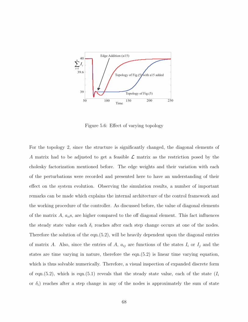
50 100 150 200 250
39
39.6
40(a15)
Topology of Fig.(5)
Topology of Fig.(5) with a15 added
Figure 5.6: Effect of varying topology
For the topology 2, since the structure is significantly changed, the diagonal elements of
A matrix had to be adjusted to get a feasible L matrix as the restriction posed by the
cholesky factorization mentioned before. The edge weights and their variation with each
of the perturbations were recorded and presented here to have an understanding of their
effect on the system evolution. Observing the simulation results, a number of important
remarks can be made which explains the internal architecture of the control framework and
the working procedure of the controller. As discussed before, the value of diagonal elements
of the matrix A, aiis, are higher compared to the off diagonal element. This fact influences
the steady state value each δi reaches after each step change occurs at one of the nodes.
Therefore the solution of the eqn.(5.2), will be heavily dependent upon the diagonal entries
of matrix A. Also, since the entries of A, aij are functions of the states Ii or Ij and the
states are time varying in nature, therefore the eqn.(5.2) is linear time varying equation,
which is thus solvable numerically. Therefore, a visual inspection of expanded discrete form
of eqn.(5.2), which is eqn.(5.1) reveals that the steady state value, each of the state (Ii
or δi) reaches after a step change in any of the nodes is approximately the sum of state
68

value before the change and a proportional component of the change. The proportionality is
directly dependent on the corresponding aiitrace(A)
or aiin∑
j=1ajj
. This analysis helps us comment on
the approximate state values after each step change which keeps the framework predictable
according to the design logic and the simulation results shown here confirms the analysis.
5.8 Overall Implementation In Power System
So far, we have developed a control framework that enables smart operation of a microgrid
during the transient active power sharing between large group of power sources distributed.
However, integrating this novel control framework with the power layer components such as
inverters, transmission line, feeders and the utility grid is also an essential task to complete
the endeavor to develop efficient microgri systems. In chapter 2, a detailed description of
existing control framework and their integration with power system layer has been described
in brief. We will attempt to conceptually integrate the newly developed control framework
with the power system layer of the grid.
Referring to the works [1, 2, 3], the power management block can be replaced with the
coupled dynamical system framework developed in this chapter, which essentially replaces
the power management calculations done by a conventional droop approach, and rest of the
system may remain same. This essentially calculates the reference values for the voltage and
speed set points for the inverters in the fig.(5.7).
69

P & Q Calculation
Low pass Filter
Low pass Filter
PI Controller
Q*
P*
+
-
+
-
a-b-cTo
q-d-n
a-b-cTo
q-d-n
Va
Vb
Vc
ea
eb
ec
Choice of Switching Vectors
PI Controller
Inverter Flux Controller
Vd
Vq
ed
eq
*
vψ
*p∂
v∂ia
ib
ic V aVb
V c
ea
eb
ec
PCC UtilityGridVSI
Feedback Measurements
ea
eb
ec
Figure 5.7: Inverter Control Scheme
The reference value for the active and reactive power here has been defined as P ∗ and Q∗
respectively. Whereas the inverter terminal voltage vectors are denoted as Va, Vb, Vc and
the voltage vectors at the PCC is denoted as ea, eb, ec. The hysteresis controller shown in
the figure, controls both the active and reactive powers, P and Q respectively, to precisely
follow the set points specified by P ∗ and Q∗. This forms the power system layer of the
microgrid. Thus from the discussions in the section 5.1, the upper and lower layer control
structure generates a reference value for the set point of the active power, for each power
sources. hence, for nth node of the network the share of active power is denoted as δn, which
acts as the reference for the active power generation P ∗n . The switching vector selection is
done using space vector pulse width modulation technique(SVPWM). For the works in [1, 2],
70

the inverter flux control has been done using a hysteresis controller and the appropriated
switching vector selection tables and analysis has been given in [63]. A similar approach is
taken for the implementation of the power system layer here in this work. Therefore, putting
all the layers together we get a complete picture of the microgrid. The lower layer is used
to manually tune or set the out put of any source as desired by the user, the upper layer
coordinated among all the power sources and distributed the load among all the sources
according to the current configuration of the graph edge weights and the power system layer
takes the reference values generated by the two layer control system and implements them
so that the load distribution follows the references. A pictorial representation of the overall
system is shown in the following figure.
71

Inverter control for nth Gen
Inverter control for 1st Gen
Inverter control for (n-1)th Gen
Two layer Control
Local Decentralized
controller
Local Decentralized
controller
Local Decentralized
controller
*nP
*1−nP
*1P
nG
1−nG
1G
Utility G
rid Bus
Utility Grid
Figure 5.8: Overall system diagram Combining power system layer and control layer
Therefore the proposed control framework demonstrates the ability to operate a microgrid
with performance specifications mentioned in the beginning of this chapter, while successfully
supplying the demanded load.
72

CHAPTER 6: CONCLUSION
The impact of the decentralized control on power grid are getting more important every
day. Considering the vision of a smart grid, the ability to plug-and-play, network flexibility,
outage management as well as the source/load side power management being the most im-
portant aspects, a decentralized framework is becoming an absolute necessity as it enables
all of the aforementioned attributes in a microgrid. The discussion so far addressed a small
scale design of a hybrid power system consisting of a SOFC and an ultra-capacitor. From
that discussion, a scaled up version of the problem, i.e for a large microgrid having a large
number of sources interconnected, the load sharing problem is addressed in a decentralized
manner using coupled autonomous systems approach, without using the expensive leader
based controller and only with local information sharing between nodes. The stability which
is a key issue with any control design was addressed in sufficient detail for both the cases. For
SOFC ultra-capacitor hybrid system, with conventional stability approaches of a differential
equation and for the coupled dynamical system approach, using reverse Cholesky factoriza-
tion method elaborated in section.5.2.2. The ability of the framework to move from one
equilibrium point to another without sacrificing performance was also demonstrated in sec-
tion.5.7. The system parameters and their effect on the performance are one fairly explored
issue however it is obvious that with the increase in the complexity of the topology, a wide
band of interesting phenomenon might appear to the surface. Some of those possibilities
were noted in respective sections of the paper. A different coupling method other than that
is demonstrated in this work might bring in some interesting outcome to the solution of this
problem. As a whole, the framework satisfies all its objectives, with promises of flexibility,
reliability and resilience.
73

APPENDIX : INPUT TO STATE STABILITY
74

According to [13], any system defined by I = f(t, I, IL), is said to be input-to-state stable
(ISS) if there exists a class KL function β and a class K function γ such that for any initial
state I(t0) and any bounded input IL(t), the solution I(t) exists for all t ≥ t0 and satisfies
‖I(t)‖ ≥ β(‖I(t0)‖, t− t0)+γ(supt0≤τ≤t ‖IL(τ)‖). A Lyapunov approach to investigating ISS
is;
Theorem: Let V : [0,∞]×Rn → R be a continuously differentiable function such that
α1(‖I‖) ≤ V (t, I) ≤ α2(‖I‖) (.1)
δV
δt+δV
δIf(t, I, IL) ≤ −W3(I), ∀‖I‖ ≥ ρ(‖IL‖) > 0, (.2)
∀(t, I, IL) ∈ [0,∞]×Rn×Rm, where α1 and α2 are class K∞ functions, ρ is a class K functions
and W3(I) is a continuous positive definite function on Rn. Then the system I = f(t, I, IL)
is input-to-state stable.
75

LIST OF REFERENCES
[1] Katiraei, F.; Iravani, M.R., ”Power Management Strategies for a Microgrid With Mul-
tiple Distributed Generation Units,” Power Systems, IEEE Transactions on , vol.21,
no.4, pp.1821,1831, Nov. 2006.
[2] Chandorkar, M.C.; Divan, D.M.; Adapa, R., ”Control of parallel connected inverters in
standalone AC supply systems,” Industry Applications, IEEE Transactions on , vol.29,
no.1, pp.136,143, Jan/Feb 1993.
[3] Katiraei,F.; Iravani,M. R.; and Lehn,P. W., ”Micro-grid autonomous operation during
and subsequent to islanding process,” IEEE Trans. Power Del., vol. 20, no. 1, pp.
248?257, Jan. 2005.
[4] Tuladhar, A.; Jin,H.; Unger,T. and Mauch,K., ”Operation of single phase inverter mod-
ules with no control interconnections,” in Proc. IEEE APEC,1997, pp. 94-100.
[5] Majumder, R.; Ghosh, A.; Ledwich, G.; Zare, F., ”Control of parallel converters for load
sharing with seamless transfer between grid connected and islanded modes,” Power and
Energy Society General Meeting - Conversion and Delivery of Electrical Energy in the
21st Century, 2008 IEEE , vol., no., pp.1,7, 20-24 July 2008.
[6] Marwali,M. N.; Jung,J.W. and Keyhani,A., ”Control of distributed generation sys-
tems”,Part II: Load sharing control,” IEEE Trans. Power Electron., vol. 19, no. 6,
pp. 1551?1561, Nov. 2004.
[7] Chen, C.; Nagananda, K.G.; Gang, X.; Kishore, S.; Snyder, L.V., ”A Communication-
Based Appliance Scheduling Scheme for Consumer-Premise Energy Management Sys-
tems,” Smart Grid, IEEE Transactions on , vol.4, no.1, pp.56,65, March 2013.
76

[8] Seon-Ju, A.; Soon-Ryul, N.; Joon-Ho, C.; Seung-Il, M., ”Power Scheduling of Dis-
tributed Generators for Economic and Stable Operation of a Microgrid,” Smart Grid,
IEEE Transactions on , vol.4, no.1, pp.398,405, March 2013.
[9] Carvalho, P.M.S.; Correia, P.F.; Ferreira, L.A.F.M., ”Distributed reactive power gener-
ation control for voltage rise mitigation in distribution networks,” IEEE Trans. Power
Syst. 23, 766?772 (2008)
[10] Zhang,H.; Lewis,F.L. and Das,A., ”Optimal design for synchronization of cooperative
systems: state feedback, observer and output feedback,” IEEE Trans. Automatic Con-
trol, vol. 56, no. 8, pp. 1948-1952, August 2011.
[11] Maknouninejad,A.; Lin,W.; Harno,H.G.; Qu,Z.; and Simaan,M.A. ”Cooperative Control
for Self-Organizing Microgrids and Game Strategies for Optimal Dispatch of Distributed
Renewable Generations,” Springer’s Journal of Energy Systems, vol.3, no.1, pp.23?60,
2012.
[12] Olfati-Saber,R.; Fax,J. and Murray,R., Consensus and cooperation in networked multi-
agent systems, Proc. IEEE, vol. 95, no. 1, pp. 215233, Jan. 2007.
[13] Khalil, H.K., Nonlinear Systems, 3rd edn. Prentice-Hall, Upper Saddle River (2002).
[14] Ching-Tai, L., ”Structural controllability,” Automatic Control, IEEE Transactions on ,
vol.19, no.3, pp.201,208, Jun 1974
[15] Meyer, Carl.D. Matrix Analysis and Applied Linear Algebra, SIAM.
[16] Smallwood, C. L., ”Distributed generation in autonomous and non-autonomous micro
grids,” inProc. IEEE Rural Electric Power Conf., May 2002, pp. D1/1D1/6.
[17] Lasseter, R. H. and Piagi, P., ”Microgrid: A conceptual solution,” in Proc. Power
Electronics specialists Conf., Aachen, Germany, Jun. 2004, vol. 6, pp. 42854290.
77

[18] Milanovic, J. V. and David, T. M., ”Stability of distributed networks with embedded
generators and induction motors,” inProc. IEEE Power Eng. Soc. Winter Meeting, New
York, Jan. 2002, vol. 2, pp. 10231028.
[19] Katiraei, F.; Iravani, M. R.; and Lehn, P. W., ”Small-signal dynamic model of a micro-
grid including conventional and electronically-interfaced distributed resources,” Proc.
Inst. Elect. Eng., Gen., Transm. Distrib.
[20] Coelho, E. A. A.; Cortizo, P. C.; and Garcia, P. F. D., ”Small-signal stability for parallel-
connected inverters in stand-alone AC supply systems,” IEEE Trans. Ind. Appl., vol.
38, no. 2, pp. 533542, Mar./Apr.2002.
[21] Ming. H; Haibing. H; Yan. X; Guerrero, J.M., ”Multilayer Control for Inverters in Par-
allel Operation Without Intercommunications,” Power Electronics, IEEE Transactions
on , vol.27, no.8, pp.3651,3663, Aug. 2012
[22] Xin, H.; Qu, Z.; Seuss, J.; Maknouninejad, A., A Self-Organizing Strategy for Power
Flow Control of Photovoltaic Generators in a Distribution Network.
[23] De Brabandere, K.; Bolsens, Bruno; Van den Keybus, J.; Woyte, A; Driesen, J.; Bel-
mans, R., ”A Voltage and Frequency Droop Control Method for Parallel Inverters,”
Power Electronics, IEEE Transactions on , vol.22, no.4, pp.1107,1115, July 2007.
[24] Majumder, R.; Ghosh, A; Ledwich, G.; Zare, F., ”Power System Stability and Load
Sharing in Distributed Generation,” Power System Technology and IEEE Power India
Conference, 2008. POWERCON 2008. Joint International Conference on , vol., no.,
pp.1,6, 12-15 Oct. 2008.
[25] Mohan, N.; Undeland, T. M.; Robbins,W. P., ”Power Electronics: Converters, Applica-
tions, and Design”,Wiley, 1989.
78

[26] Sinden,G., ”Assessing the Costs of Intermittent Power Generation”, UK Energy Re-
search Centre, 5 July 2005.
[27] Kuntz, M. T.; Dawe, J. , ”renewable. rechargeable. remarkable.”. VRB Power Systems.
Mechanical Engineering. Retrieved 2008-10-20.
[28] Samantha, .; Sims, R. and Kirchner, N., ”Contribution of renewables to energy security.”
IEA Information Paper (2007).
[29] Karlsson, P. and Svensson, J., DC bus voltage control for a distributed power system,
IEEE Trans. Power Electron., vol. 18, no. 6, pp. 14051412, Nov. 2003.
[30] Lu, X.; Sun, K.; Guerrero, J. M.; Vasquez, J. C.; Huang, L. and Teodorescu, R., SoC-
based droop method for distributed energy storage in dc Microgrid applications, in Proc.
IEEE Int. Symp. Ind. Electron.(ISIE), 2012, pp. 16401645.
[31] Ferreira, R. A. F.; Braga, H. A. C.; Ferreira, A. A. and Barbosa, P. G., Analysis of
voltage droop control method for dc Microgrids with Simulink: modeling and simulation,
in Proc. 10th IEEE/IAS Int. Conf. Ind. Appl. (INDUSCON), 2012, pp. 16.
[32] Lopes, J. A. P.; Moreira, C. L. and Madureira, A. G., Defining control strategies for
Microgrids islanded operation, IEEE Trans. Power Syst., vol. 21, no. 2, pp. 916924, May
2006.
[33] Kundur, P., Power System Stability and Control, McGraw-Hill Education, (1994).
[34] Hornik, T.; Zhong,Q. C., ”A Current-Control Strategy for Voltage-Source Inverters in
Microgrids Based on H∞ and Repetitive Control,” Power Electronics, IEEE Transac-
tions on , vol.26, no.3, pp.943,952, March 2011.
79

[35] Lennart, A.; Lindberg, L., ”Inner phase angle control of voltage source converter in high
power applications,” Power Electronics Specialists Conference, 1991. PESC ’91 Record.,
22nd Annual IEEE , vol., no., pp.293,298, 24-27 Jun 1991.
[36] Rodriguez, J.; Pontt, J.; Silva, C.A; Correa, P.; Lezana, P.; Cortes, P.; Ammann, U.,
”Predictive Current Control of a Voltage Source Inverter,” Industrial Electronics, IEEE
Transactions on , vol.54, no.1, pp.495,503, Feb. 2007.
[37] Abu-Rub, H.; Guzinski, J.; Krzeminski, Z.; Toliyat, H. A, ”Predictive current control
of voltage source inverters,” Industrial Electronics Society, 2001. IECON ’01. The 27th
Annual Conference of the IEEE , vol.2, no., pp.1195,1200 vol.2, 2001.
[38] Lin, C.T., ”Structural controllability.” Automatic Control, IEEE Transactions on 19.3
(1974): 201-208.
[39] Vandoorn, T., et al. ”A voltage-source inverter for microgrid applications with an inner
current control loop and an outer voltage control loop.” International Conference on
Renewable Energies, and Power Quality (ICREPQ09). 2009.
[40] Ford, G. W. and Uhlenbeck, G. E., ”Combinatorial Problems in the Theory of Graphs
III.” Proc. Nat. Acad. Sci. USA 42, 529-535, 1956.
[41] Allag, T.; Das, T., ”Robust Control of Solid Oxide Fuel Cell Ultracapacitor Hybrid
System,” Control Systems Technology, IEEE Transactions on , vol.20, no.1, pp.1,10,
Jan. 2012.
[42] Das, T.; Snyder, S., ”Adaptive Control of a Solid Oxide Fuel Cell Ultra-Capacitor
Hybrid System,” Control Systems Technology, IEEE Transactions on , vol.21, no.2,
pp.372,383, March 2013.
80

[43] Greenwell, W.; Vahidi, A, ”Predictive Control of Voltage and Current in a Fuel Cel-
lUltracapacitor Hybrid,” Industrial Electronics, IEEE Transactions on , vol.57, no.6,
pp.1954,1963, June 2010.
[44] Drolia, A; Jose, P.; Mohan, N., ”An approach to connect ultracapacitor to fuel cell
powered electric vehicle and emulating fuel cell electrical characteristics using switched
mode converter,” Industrial Electronics Society, 2003. IECON ’03. The 29th Annual
Conference of the IEEE , vol.1, no., pp.897,901 vol.1, 2-6 Nov. 2003.
[45] Single 9-a high-speed low-side mosfet driver with enable.
http://www.ti.com/lit/ds/slusa13b/ slusa13b.pdf.
[46] http://greenlightnational.com/why-colleges-are-big-believers-in-microgrids/
[47] Majumder, R.; Ghosh, A; Ledwich, G.; Zare, F., ”Angle droop versus frequency droop
in a voltage source converter based autonomous microgrid,” Power & Energy Society
General Meeting, 2009. PES ’09. IEEE , vol., no., pp.1,8, 26-30 July 2009.
[48] Slootweg, J.G.; Kling, W.L., ”Impacts of distributed generation on power system tran-
sient stability,” Power Engineering Society Summer Meeting, 2002 IEEE , vol.2, no.,
pp.862,867 vol.2, 25-25 July 2002.
[49] Donnelly, M.K.; Dagle, J.E.; Trudnowski, D.J.; Rogers, G.J., ”Impacts of the distributed
utility on transmission system stability,” Power Systems, IEEE Transactions on , vol.11,
no.2, pp.741,746, May 1996.
[50] Ganguly, S., Sahoo, N. C. and Das, D., ”A novel multi-objective PSO for electrical
distribution system planning incorporating distributed generation.” Energy Systems
1.3 (2010): 291-337.
81

[51] Carvalho, P. M S; Correia, Pedro F.; Ferreira, L.AF., ”Distributed Reactive Power Gen-
eration Control for Voltage Rise Mitigation in Distribution Networks,” Power Systems,
IEEE Transactions on , vol.23, no.2, pp.766,772, May 2008.
[52] Masters, C. L., ”Voltage rise: the big issue when connecting embedded generation to
long 11 kV overhead lines,” Power Engineering Journal , vol.16, no.1, pp.5,12, Feb.
2002.
[53] Bollen, M. H J; Sannino, A, ”Voltage control with inverter-based distributed genera-
tion,” Power Delivery, IEEE Transactions on , vol.20, no.1, pp.519,520, Jan 2005.
[54] Jancke, G.; Fahlen, N.; Nerf, O., ”Series capacitors in power systems,” Power Apparatus
and Systems, IEEE Transactions on , vol.94, no.3, pp.915,925, May 1975.
[55] Iliceto, F.; Cinieri, E., ”Comparative analysis of series and shunt compensation schemes
for AC transmission systems,” Power Apparatus and Systems, IEEE Transactions on ,
vol.96, no.6, pp.1819,1830, Nov. 1977.
[56] Li, Y. W.; Kao, C. N., ”An Accurate Power Control Strategy for Power-Electronics-
Interfaced Distributed Generation Units Operating in a Low-Voltage Multibus Micro-
grid,” Power Electronics, IEEE Transactions on , vol.24, no.12, pp.2977,2988, Dec. 2009.
[57] Zhou, H.; Bhattacharya, T.; Duong .T; Siew, T.S.T.; Khambadkone, AM., ”Composite
Energy Storage System Involving Battery and Ultracapacitor With Dynamic Energy
Management in Microgrid Applications,” Power Electronics, IEEE Transactions on ,
vol.26, no.3, pp.923,930, March 2011.
[58] Hines, P.; Talukdar, S., ”Reciprocally altruistic agents for the mitigation of cascading
failures in electrical power networks,” Infrastructure Systems and Services: Building
82

Networks for a Brighter Future (INFRA), 2008 First International Conference on , vol.,
no., pp.1,6, 10-12 Nov. 2008.
[59] McArthur, S.D.J.; Davidson, E.M.; Catterson, V.M.; Dimeas, AL.; Hatziargyriou, N.D.;
Ponci, F.; Funabashi, T., ”Multi-Agent Systems for Power Engineering ApplicationsPart
I: Concepts, Approaches, and Technical Challenges,” Power Systems, IEEE Transactions
on , vol.22, no.4, pp.1743,1752, Nov. 2007.
[60] Dorfler, F.; Jovanovic, M.R.; Chertkov, M.; Bullo, F., ”Sparse and optimal wide-area
damping control in power networks,” American Control Conference (ACC), 2013 , vol.,
no., pp.4289,4294, 17-19 June 2013.
[61] Yih-Fang. H; Werner, S.; Jing Huang; Kashyap, N.; Gupta, V., ”State Estimation in
Electric Power Grids: Meeting New Challenges Presented by the Requirements of the
Future Grid,” Signal Processing Magazine, IEEE , vol.29, no.5, pp.33,43, Sept. 2012.
[62] http://www.energy.gov/
[63] Takahashi, I; Noguchi, T., ”A New Quick-Response and High-Efficiency Control Strat-
egy of an Induction Motor,” Industry Applications, IEEE Transactions on , vol.IA-22,
no.5, pp.820,827, Sept. 1986.
[64] Guo, Y., Hill, D. J., and Wang, Y., ”Nonlinear decentralized control of large-scale power
systems,” Automatica, 36(9), 1275-1289, 2000.
[65] Ugrinovskii. V and Pota. H, ”Decentralized control of power systems via robust control
of uncertain markov jump parameter systems,” In Proceedings of 43rd IEEE Conference
on Decision and Control, pages 35033508, December 2004.
[66] Aquino-Lugo. A, ”Distributed and decentralized control of the power grid,” PhD thesis,
University of Illinois at Urbana-Champaign, 2011.
83

[67] Tuladhar, A.; Jin, K.; Unger, T.; Mauch, K., ”Parallel operation of single phase inverter
modules with no control interconnections,” Applied Power Electronics Conference and
Exposition, 1997. APEC ’97 Conference Proceedings 1997., Twelfth Annual , vol.1, no.,
pp.94,100 vol.1, 23-27 Feb 1997.
[68] Hines, P.; Talukdar, S., ”Reciprocally altruistic agents for the mitigation of cascading
failures in electrical power networks,” Infrastructure Systems and Services: Building
Networks for a Brighter Future (INFRA), 2008 First International Conference on , vol.,
no., pp.1,6, 10-12 Nov. 2008.
[69] Haddad, M.M.; Hui, Qing; Chellaboina, V.; Nersesov, S.G., ”Hybrid decentralized max-
imum entropy control for large-scale dynamical systems,” American Control Conference,
2006 , vol., no., pp.6 pp.,, 14-16 June 2006.
[70] Ramakrishna, A.; Viswanadham, N., ”Decentralized control of interconnected dynam-
ical systems,” Decision and Control including the Symposium on Adaptive Processes,
1980 19th IEEE Conference on , vol., no., pp.538,543, 10-12 Dec. 1980.
[71] Bakule. L, Decentralized control: An overview. Annual Reviews in Control, 32(1):87
98, 2008.
84