Decision-Making under Subjective Risk:Toward a General Theory of Pessimism∗

Anna Gumen† Efe A. Ok‡ Andrei Savochkin§

March 20, 2014

Abstract

The primary objective of this paper is to develop a framework in which a decision-maker may have subjective beliefs about the “riskiness” of prospects, even though therisk structure of these prospects is objectively specified. Put differently, we investigatepreferences over risky alternatives by postulating that such preferences arise from morebasic preferences that act on the subjective transformations of these prospects. Thisallows deriving a theory of preferences over lotteries with distorted probabilities andprovides information about the structure of such distortions. In particular, we are ableto formulate a behavioral trait such as “pessimism” in the context of risk (independentlyof any sort of utility representation) as a particular manifestation of the uncertaintyaversion phenomenon. Our framework also provides a strong connection between thenotions of aversion to ambiguity and risk which are regarded as distinct traits in decisiontheory.

JEL Classification: D11, D81.Keywords: Distortion of Probabilities, Pessimism/Optimism, Non-Expected Utility The-ory, Uncertainty Aversion, Risk Aversion.

∗We thank David Dillenberger, Paolo Ghirardato, Sujoy Mukerji, Pietro Ortoleva and Peter Wakker, aswell as the participants of the seminars given at Cal Tech, Cambridge University, Florida State, NES-Moscow,LBS, NYU, Oxford and Rutgers.

†Department of Economics, New York University. E-mail: anna.gumen@nyu.edu.‡Department of Economics, New York University, 19 West 4th Street, New York, NY 10012. E-mail:

efe.ok@nyu.edu.§Collegio Carlo Alberto, Via Real Collegio 30, 10024 Moncalieri (TO), Italy. E-mail:

andrei.savochkin@carloalberto.org.

1

Suam habet fortuna rationem.1

Petronius

1 Introduction

Motivation. We hear the following types of statements routinely in daily discourse:

“Roll the dice, I feel lucky today.”

“I’m really not lucky when it comes to slot machines.”

“There was 10% chance I could lose, but I knew I would.”

There are even commonly used narratives such as “Murphy’s law,” or “50-50-90 rule: If thechance of something good happens is 50-50, then something bad happens 90% of the time.”

It is, of course, important to understand the behavior of people who say such things andmake decisions accordingly, at least from a descriptive viewpoint. Yet, to a rational decisiontheorist, it is not an easy matter to make sense of such sentiments, and even to take themseriously. After all, a toss of a fair coin that pays $10 if heads come up and -$5 otherwise,is supposed to be just that; a probability distribution p with p(−5) = 1

2 = p(10), whoeverplays it. It is not that decision theorists are strangers to traits like pessimism or optimism,but those notions are readily meaningful only when there is room for subjective assessmentof likelihoods of outcomes, not when these likelihoods are provided in an objective sense. Inthe example of a toss of a fair coin, probabilities are presumed to be known – the situation isone of risk, not of uncertainty, to use the distinction made famously by Frank Knight.

One sensible way out of this conundrum is to recognize that an individual holds the rightto subjectively evaluate the likelihood of outcomes in a lottery even though she understandsthat these likelihoods are indeed objectively given. This evaluation will, of course, take theobjectively given probabilities into account, but it does not have to yield “beliefs” that matchthese probabilities exactly. To wit, in the fair coin tossing example above, we propose to thinkof an individual as one who is facing an act f on the state space H, T with f(H) = 10 andf(T ) = −5. What distinguishes this from a purely Savagean outlook is that the individual hasthe information that the (objective) probabilities of H and T are 1

2 . Put differently, while thevon Neumann-Morgenstern formulation of this bet is µ, the uniform probability distributionon H, T, and the purely Savagean formulation of it is simply f (that would model a situationin which nothing is known about the likelihood of outcomes), we propose that the individuallooks at this bet in a hybrid way as (µ, f).2

In a nutshell, the main goal of the present paper is to investigate preferences over (objec-tive) risky prospects by postulating that such preferences arise from more basic preferencesthat act on the subjective transformations of these prospects. As we shall see, this approachallows one to “derive” a theory of preferences over lotteries with distorted probabilities, andprovides information about the structure of such distortions.

1Chance has its reasons.2To illustrate, in Figure 1, the left-most part represents the von Neumann-Morgenstern formulation of this

lottery, the center one the purely Savagean formulation, and the right-most part corresponds to the hybridformulation we propose here.

2

10

−5

1/2

1/2

!

!

!

10

−5

Heads

Tails

!

!

!

10

−5

Heads (1/2)

Tails (1/2)

!

!

!

Figure 1

The idea of “distorted probabilities” is, of course, not new. It dates back at least to theworks of Preston and Baratta (1948) and Edwards (1954) in psychology, and Kahneman andTversky (1979) in economics. Indeed, non-expected utility theory provides a number of modelsin which the decision maker evaluates a lottery by means of an expected utility computation,one in which probabilities of outcomes are not necessarily the ones given in the lottery. Thereis, however, a major difference between our approach and non-expected utility theory. Thelatter theory does not have room for looking at these probability distortions at the level ofprimitives. Instead, it derives them by means of structural postulates that weaken the classicalindependence axiom (so that the theory conforms with the Allais paradox, common ratioeffect, etc.), thereby providing behavioral tests for checking whether or not these distortionstake place in some consistent manner. While it is obviously useful, this approach does notattribute any behavioral meaning to such distortions, they are meaningful only within specificmodels. As we shall see, this makes it quite difficult to talk about traits such as pessimismor optimism at a general level. By contrast, what we wish to do in this paper is to allow anagent to view his “luck” as different than the objectively given probabilities at the level ofprimitives (not only as an interpretation of the representation of the preferences). In otherwords, we introduce the possibility of subjective evaluation of the likelihood of outcomes ina lottery at the modeling stage, thereby giving a Savagean outlook to risk preferences; hencethe term subjective risk preferences. This approach permits the analyst to look at distortedprobabilities of non-expected utility theory as the “beliefs” of the decision maker about thevarious outcomes of a given lottery. As such, it builds a bridge through which the insightsobtained in the theory of decision-making under uncertainty can be carried into the realm ofchoice under risk.

An Outline of the Subjective Risk Model. In Section 2, we introduce the main ingredients ofour model. First, we introduce a natural state space Ω that allows one to view any givenmonetary lottery as an act. (A state describes what occurs in every lottery in the world,providing a complete resolution of uncertainty.) The objectively given probabilities of a lotteryinduce a probability distribution on a (finite) partition of Ω. Consequently, every lottery pis transformed into what we call a degenerate info-act, (µ, f), where f takes value x in allstates where x is the outcome of p, and µ is a probability distribution on Ω that tells us theprobability of the event that “x is the outcome of p” is p(x). Second, we postulate that thedecision maker has preferences over all degenerate info-acts, and she prefers one lottery overanother iff she prefers the info-act that corresponds to the former lottery to the info-act thatcorresponds to the latter.

This is, of course, nothing but relabelling so far. Next, to get some mileage from the

3

approach, we extend the notion of a degenerate info-act into what we simply call an info-act(µ, f), by allowing f to pay out consequences other than the payoffs of the involved lotterywhen a state is realized. (Such an info-act pays a particular consequence (which need not bex) in the event that “x is the outcome of p”.) To make use of the Anscombe-Aumann theory,we take such consequences themselves as lotteries, and hypothesize that the agent has well-defined preferences over these info-acts as well. This way, the space of lotteries embeds in thespace of info-acts (but the latter is much larger than the former), and we can read off one’s riskpreferences from her preferences over info-acts (by looking at how she ranks degenerate info-acts), but not conversely. In fact, under an unexceptionably weak monotonicity hypothesis, weshow that the latter preferences yield risk preferences that are represented by expected utility,albeit, with distorted probabilities (Proposition 1). It is in this sense that the subjective risktheory “derives” the distortions of likelihood of outcomes in a lottery from the preferences ofa person under uncertainty.3

One way of thinking about preferences over info-acts is as the “model of the mind” ofthe agent in the context of the evaluation of uncertainty in general. Then, if one is preparedto make some general assumptions on the structure of this “model of the mind,” we maygather insights in terms of the risk preferences of the agent. For instance, the first mainresult of this paper shows that, under a standard monotonicity hypothesis, whether or nota decision maker distorts objective probabilities (and then use the distorted probabilities tomake expected utility computations) depends vitally on her attitude toward ambiguity. Putmore concretely, ambiguity neutrality of a decision maker ensures that this person does notdistort the probabilities and acts as a standard expected utility maximizer (Theorem 2). Ina formal sense, therefore, our approach entails that probability distortions of non-expectedutility theory can be seen to arise from one’s lack of neutrality toward ambiguity, therebyallowing a viewpoint in which the Allais paradox emerges as a “special case” of certain typesof the Ellsberg paradox. (Notably, this statement cannot even be formulated in the contextof non-expected utility theory.)

Pushing this point further, we can also deduce certain properties of one’s risk preferencesfrom her attitudes toward uncertainty. In particular, we prove in Theorem 9 that risk aver-sion that is caused by probability distortions is a consequence of one’s uncertainty aversionat large (in the sense that if one’s subjective risk preferences are uncertainty averse, thenthe corresponding risk preferences must be (probabilistically) risk averse). This observationbrings together two empirically meaningful phenomena, uncertainty aversion and risk aversion,which exist in formally disparate realms, through subjective risk theory. It makes it formallymeaningful to assert that one’s (probabilistic) risk aversion is a consequence of her ambiguityaversion (again a statement that cannot be formulated in the context of non-expected utilitytheory).

A General Formulation of Pessimism for Risk Preferences. A major advantage of the “subjective

3A quick remark about the observability of preferences over info-acts is in order. It is plain that one cannotidentify the entirety of the preferences of a person over info-acts from her choices over risky prospects; thelatter type of choices identify only the part of these preferences over degenerate acts. Consequently, insofarthe analysis is confined only to lottery choices, preferences over info-acts are only partially observable. Butthis does not mean that such preferences are rather artificial. As info-acts are observable objects, one can askan agent directly to rank info-act pairs, thereby deducing her info-act preferences completely.

4

risk” approach is to allow the analyst to formulate certain subjective behavioral traits, suchas pessimism, in the context of risk. Pessimism is viewed in non-expected utility theory assome form of over(under)weighting of the probability of bad (good) outcomes; it is commonlydefined for the general weighted EU model by using the probability weighting function ofthat model. Unfortunately, due to the non-uniqueness of probability weighting functions thatrepresent a preference relation as in that model, this way of defining pessimism is behaviorallymeaningful only in some special cases of the general weighted EU model with strong unique-ness properties. In particular, this definition (given formally in Section 4.3) is behaviorallymeaningful, and it delivers an intuitively appealing conceptualization of pessimism in the con-text of rank-dependent utility (RDU) model. Yet, even when it is meaningful, this approachturns out to be rather coarse. For instance, as we prove in Proposition 8, in the context ofdisappointment averse preferences of Gul (1991), this way of looking at pessimism fails toclassify any preference as pessimistic or optimistic, other than the trivial case of expectedutility preferences.

It is important to note that such difficulties do not arise in the context of choice underuncertainty. Indeed, in that context, there is already a widely used notion of pessimism inthe context of uncertainty; this is the notion of uncertainty aversion (that is, preference forhedging). Roughly speaking, what we propose to do here is to classify a risk preference aspessimistic if that preference is the projection of an uncertainty averse preference over the info-acts. As we explain in some detail in Section 4.1, there are also difficulties in this approachrelated to non-uniqueness, for, in general, one cannot in general identify one’s preferences overinfo-acts from her (observable) risk preferences. However, if one is prepared to make somegeneral assumptions on the structure of the presumed “model of the mind,” that is, on one’spreferences over info-acts, the difficulty may be circumvented. In particular, if we restrict ourattention to a class of preferences over info-acts that are uniquely identified by their restrictionto the set of degenerate info-acts – such a class of preferences is called viable in this paper –we do achieve a one-to-one correspondence between one’s risk preferences and her preferencesover info-acts, and our definition of pessimism becomes behaviorally meaningful. So long aswe speak relative to a given viable class, we can talk rigorously about the pessimism of a givenrisk preferences. And, fortunately, there are many viable classes, and some of these are quiterich in content. For instance, as we show in the body of the paper, if we focus on agents whocompare two info-acts of the form (µ, f) and (µ, g) according to, say, maxmin, or maxmax, orChoquet, preferences, or a convex combination of these (as in the α-maxmin model), or moregenerally, according to what is called biseparable expected utility, then we obtain a viableclass (Proposition 3). Similarly, the class of c-neutral preferences, that is, the collection ofmonotone preferences over info-acts which evaluate constant acts in a risk neutral manner, isviable (Proposition 4).

We demonstrate the usefulness of this approach toward pessimism by means of concreteexamples. First, we show that our definition (relative to the viable class of biseparable pref-erences) agrees completely with the way literature defines pessimism in the context of RDUmodel (Proposition 5). Second, we show that this definition is significantly more refined thanthe latter definition. For instance, unlike the definition of pessimism in terms of probabilityweighting functions, we show in Proposition 6 that our definition of pessimism correspondsprecisely to disappointment aversion in the context of Gul’s model, sitting square with thetypical way this model is interpreted. In a related application, we show in Proposition 7 that a

5

cautious expected utility preference (cf. Cerreia-Vioglio, Dillenberger and Ortoleva (2013)) ispessimistic (relative to the viable class of c-neutral preferences) if and only if it is risk averse.The definition of pessimism through non-expected utility theory does not even apply to thismodel in a natural manner.

Intuitively, a “pessimistic person” would be particularly nervous about passing an oppor-tunity of spreading the risk in her investments, in a way that may go beyond what risk aversionwould account for. Indeed, an RDU preference that is pessimistic according to the standarddefinition would always look to diversifying her portfolio, even if her utility for money is alinear function. Unfortunately, this observation does not extend beyond this model. For in-stance, if pessimism is defined through weight distortions in a similar fashion in Gul’s model,then it would not imply preference for diversification. By contrast, the final result of thepresent paper shows that the notion of pessimism we have introduced here (with respectto c-neutral preferences over info-acts) is generally consistent with intuition in this regard.Loosely speaking, we prove in Theorem 11 that, with our definition, every pessimistic person(with linear utility for money) exhibits preference for diversification. This property accordswell with what one would intuitively expect from the behavior of a “pessimistic person,” andhence provides further support for the general formulation we advance here.

2 Formulation of Risk as Uncertainty

The purpose of this section is to describe a model that modifies the standard framework ofpreferences over monetary lotteries to allow for subjective evaluation of “objective risk.”

2.1 Nomenclature

We begin by introducing the order-theoretic nomenclature that is used in what follows. Forany nonempty set S, by a preference relation ! on S we mean a reflexive and transitivebinary relation on S. The asymmetric (strict) part of ! is denoted as ≻, and its symmetric(indifference) part is denoted as ∼. For any nonempty subset T of S, by the restriction of! to T, we mean the binary relation ! |T := ! ∩ (T × T ). We say that ! is complete tomean that either s ! t or t ! s holds for every s, t ∈ S. A real function V on S is said torepresent ! if it is a utility function for !, that is, s ! t iff V (s) ≥ V (t), for every s, t ∈ S.When S is a topological space, we say that a preference relation ! on S is continuous if itis a closed subset of S × S (relative to the product topology).

2.2 The State Space induced by Lotteries

The Lottery Space. We focus throughout this paper on monetary lotteries and/or acts withmonetary payoffs. Consequently, even though parts of the discussion below apply in a moregeneral context, we shall designate here a nondegenerate compact interval X in R as theoutcome space of the model. By a simple lottery on X , we mean a Borel probabilitymeasure on X with finite support. The expectation of a continuous real map v on X withrespect to a simple lottery p on X is denoted by E(v,p), but we write E(p) when v is theidentity map on X .

6

The set of all simple lotteries on X is denoted as (X). As usual, we view (X) as atopological space relative to the topology of weak convergence: A net (pα) in (X) convergesto a simple lottery p on X iff E(v,pα) → E(v,p) for every continuous real map v on X.Finally, the degenerate Borel probability measure on X that yields x with probability one isdenoted as δx; we refer to such a measure as a degenerate lottery.

Preferences over Lotteries. We consider here only the complete and continuous preferencerelations on (X). In addition, we always presume that money is a desirable commodity, sowe posit at the outset that δx ! δy iff x ≥ y, for every x, y ∈ X. The set of all such preferencerelations on (X) is denoted by R(X).

The State Space. To describe the “subjective evaluation” of lotteries that we propose, the firststep is designating a suitable state space. We will use for this purpose the set of all functionsfrom (X) into X that map each lottery to an element of its support. That is, we designateas our state space the set

Ω :=

ω ∈ X(X) : ω(p) ∈ supp(p) for each p ∈ (X)

.

In words, Ω consists of the descriptions of all contingencies that may result when a personplays any one simple lottery on X. Put differently, a state ω in Ω describes what preciselyhappens in every lottery in the world, and hence, in concert with the Savagean modeling ofuncertainty, represents the complete resolution of uncertainty.4

For any given lottery p ∈ (X) and x ∈ supp(p), we let

Ω(p, x) := ω ∈ Ω : ω(p) = x,

which is the event that “the outcome x obtains in the lottery p.” Then, Ω(p) := Ω(p, x) : x ∈supp(p) is a (finite) partition of the state space Ω that corresponds to the uncertaintyembodied in p.

Info-Acts. Suppose p is the lottery that corresponds to the tossing of a fair coin, one thatpays $10 if Heads come up and −$5 otherwise. As we have noted in the Introduction, wepropose to view this lottery as an act that pays a sure payoff of $10 in the event “Headscome up in the toss,” and −$5 in the event “Tails come up in the toss,” together with theinformation that these events are equally likely. Assuming that −5 and 10 belong to X, ourformulation captures the event “Heads come up in the toss,” by Ω(p, 10), and the event “Tailscome up in the toss,” by Ω(p,−5). Thus, we let an agent conceive p as a (Savagean) act onΩ, say, f, one that pays $10 at any state in Ω(p, 10), and −$5 at any other state in Ω. Theagent is, however, aware that these events are equally likely, that is, she is given a probabilitydistribution over the partition Ω(p) that assigns probability 1

2 to the event Ω(p, 10). Denotingthis particular distribution by µ, therefore, we model the objective lottery p as the pair (µ, f),thereby allowing the decision maker to look at things subjectively.

We now formalize this idea. For any p in (X), let us denote by ⟨p⟩ the probabilitymeasure on the algebra generated by Ω(p) on Ω such that ⟨p⟩(Ω(p, x)) = p(x) for each x

4Once X is specified, Ω is uniquely defined. To simplify the notation, however, we do not use a notationthat makes the dependence of Ω on X explicit.

7

in supp(p). In turn, we denote by F(p), the set of all (X)-valued acts on F(p), that is,the set of all maps f : Ω → (X) that are measurable with respect to this algebra. Putdifferently, f ∈ F(p) iff f is a map from Ω into (X) that is constant on each element of thepartition Ω(p). If every value of f ∈ F(p) is a degenerate lottery, that is, f(Ω) is containedin δx : x ∈ X, we say that f is degenerate-valued. A particularly important degenerate-valued act in F(p) is the one that pays exactly what p pays on the event that “the outcomex obtains in the lottery p.” Throughout this paper, we denote this act by fp: Put explicitly,fp is the act on Ω such that f |Ω(p,x) = δx for every x ∈ supp(p), that is,

fp =∑

x∈supp(p)

δx1Ω(p,x).

Convention. For any p ∈ (X), f ∈ F(p) and x ∈ supp(p), we denote “the” value of f onΩ(p, x) by f(x) throughout the exposition. That is, we set f(x) := f(ω) for some (and henceany) ω in Ω(p, x).5

By an info-act on Ω, we mean an ordered pair (⟨p⟩, f) where p is a simple lottery on Xand f ∈ F(p). We denote the set of all info-acts by #(X), that is,

#(X) := (⟨p⟩, f) : p ∈ (X) and f ∈ F(p).

A degenerate info-act on Ω is a member (⟨p⟩, f) of #(X) such that f is a degenerate-valued act on F(p). A particularly important such info-act is (⟨p⟩, fp), which we refer to asthe info-act on Ω induced by p. The idea is that, when evaluating a lottery p, which is arisky prospect, the agent feels like she actually faces an uncertain prospect. She knows thatthis prospect will pay her x in the “event Ω(p, x),” as well as the fact that the “event Ω(p, x)”is declared to obtain with probability p(x). So, the image of the lottery p in her mind isprecisely the info-act (⟨p⟩, fp).

There are various ways of turning #(X) into a topological space. We do this by endowing#(X) with a topology that is intuitively consistent with the weak convergence of probabilitymeasures: We say that a net (µα, fα) in #(X) converges to an info-act (µ, f) on Ω iff

∫

Ω

E(v, fα(·)) dµα →

∫

Ω

E(v, f(·)) dµ

for every continuous real map v on X.Before we proceed further, let us point to a caveat. Notice that the codomain of f in

any info-act (µ, f) is (X), instead of X, that is, “acts” are modeled here as the Anscombe-Aumann horse-race lotteries, as opposed to Savagean acts. While taking a purely Savageanapproach would intuitively be more appropriate for the present exercise, that approach ismarred with considerable technical complications. This is, of course, typical in decision theory.Indeed, a vast majority of the recent developments in the theory of decision making underuncertainty exploits the richer structure of the Anscombe-Aumann framework instead of the

5In other words, we define f : supp(p) → ∆(X) by f(x) := f(ω) for some (and hence any) ω in Ω(p, x),and as a convention, identify f with f .

8

Savagean one. For tractability reasons on one hand, and because we will make subsequent useof these developments on the other, we also adopt this framework in the present paper.

Interpretation of Info-Acts. #(X) provides a setting for talking about subjective risk. Theobservable framework is the standard one in which a decision-maker ranks monetary lotteries.The upshot here is that the decision-maker need not take the probabilities in a given lotteryas declared. Instead, she uses these probabilities as information about the likelihood of theoutcomes of the lottery, and may form beliefs about these likelihoods that differ from what isprescribed by the lottery. To wit, if p is a simple lottery on X , then the agent actually viewsthis lottery as the info-act (⟨p⟩, f), where ⟨p⟩(Ω(p, x)) = p(x) and f(ω) = δx for every ω ∈ Ωwith ω(p) = x.

Preferences over Info-acts. We consider here only the complete and continuous preferencerelations on #(X). Besides, we presume that a person with a preference relation ! on #(X)prefers more money to less regardless of the information she is given about the likelihood ofvarious states, that is, we posit at the outset that (⟨p⟩, δx1Ω) ! (⟨p⟩, δy1Ω) iff x ≥ y, for everyx, y ∈ X and p ∈ (X). (This property is referred to as the “desirability of money” in whatfollows.)6

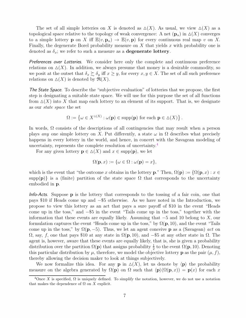
State-Invariance. The set of all info-acts on Ω contains some redundancies. That is, it containsinfo-acts that one cannot distinguish from each other behaviorally. This necessitates imposingcertain invariance properties on the preferences over info-acts. For instance, consider a lotteryp that pays $1 with probability 1

6 , $2 with probability 13 , and $3 with probability 1

2 , and anact f in F(p) which pays a lottery ai in the event Ω(p, i), i = 1, 2, 3. Now compare thiswith the info-act (⟨q⟩, g), where q is the lottery that pays x1 with probability 1

6 , x2 withprobability 1

3 , and x3 with probability 12 , and g is that act in F(q) which pays ai in the event

that the outcome xi obtains in the lottery q. It is clear that the difference between the info-acts (⟨p⟩, f) and (⟨q⟩, g) is immaterial. Indeed, these info-acts partition the state space intothree events, say, A1, A2, A3 and B1, B2, B3, respectively, and inform the decision-makerthat the probabilities of Ai and Bi are the same for each i = 1, 2, 3. (Here, Ai = Ω(p, i) andBi = Ω(q, xi) for each i.) Furthermore, the payoff of (⟨p⟩, f) in the event Ai and that of(⟨q⟩, g) in the event Bi are the same, namely, ai, for each i. Clearly, while the formalism of themodel treats (⟨p⟩, f) and (⟨q⟩, g) as different objects, the interpretation of it would cease tomake sense if we allowed an individual perceive these info-acts as such. We must, therefore,impose on a preference relation ! a “state anonymity” condition that says that preferencesare invariant under the renaming of states, thereby ensuring that (⟨p⟩, f) ∼ (⟨q⟩, g). (SeeFigure 2.)

There is another situation that requires imposing a similar invariance condition. Indeed,our interpretation requires an agent not distinguish between two info-acts (µ, f) and (ν, f) solong as f is a constant act. More generally, we should make sure that the given probabilities

6Insofar as the primitives of the model are lotteries, and hence info-acts are the analyst’s constructs, wecannot determine one’s preferences over non-degenerate info-acts from her risk preferences. It is in this sensethat preferences over info-acts are not observable. Having said this, info-acts are concrete objects, and wecan certainly determine an individual’s preferences over them by asking her to compare such objects (say, inexperimental settings). Thus, potentially, albeit, not from the ranking of lotteries, preferences over info-actsare observable entities.

9

16

13

12

f = a1

f = a2

f = a3

Ω

∼

16

13

12

g = a1

g = a2

g = a3

Ω

Figure 2: The State Anonymity Property

16

13

12

f = a1

f = a2

f = a3

Ω

∼

16

13

14

14

g = a1

g = a2

g = a3

g = a3

Ω

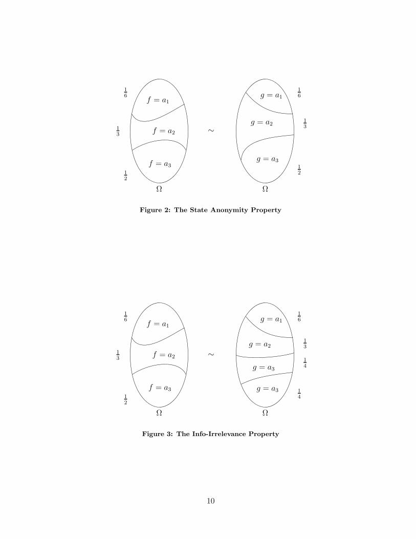
Figure 3: The Info-Irrelevance Property

10

of any two states are immaterial for preferences in evaluating an act that yields the sameoutcome on those two states (other than what they entail for the likelihood of those twostates put together). To illustrate, let (⟨p⟩, f) be as above and consider the info-act (⟨q⟩, g)where Ω(q) = B1, ..., B4 and ⟨q⟩ assigns probability 1

6 to B1,13 to B2,

14 to B3, and

14 to

B4, while g pays ai in the event Bi, i = 1, 2, and a3 in the event B3 ∪ B4. It is clear thatthe difference between (⟨p⟩, f) and (⟨q⟩, g) is immaterial for choice, so we must impose aninvariance condition that ensures that (⟨p⟩, f) ∼ (⟨q⟩, g). (See Figure 3.)

We thus introduce the following property on one’s preferences over info-acts that providesa joint formalization of these two invariance properties.

The State Invariance Axiom. Let (⟨p⟩, f) and (⟨q⟩, g) be two info-acts on Ω for which thereis a map σ : Ω(q) → Ω(p) such that

(i) f(ω′) = g(ω) for every S ∈ Ω(q) and (ω,ω′) ∈ S × σ(S); and(ii) ⟨q⟩(σ−1(T )) = ⟨p⟩(T ) for every T ∈ σ(Ω(q)).

Then, it must be that (⟨p⟩, f) ∼ (⟨q⟩, g).

The set of all complete and continuous preference relations on #(X) that satisfy thedesirability of money and State Invariance Axioms is denoted by P(X).

Related Models. To the best of our knowledge, preferences over prior-act pairs (that is, info-acts) have not been considered in the literature. Work that comes closest to doing this pertainto ranking ordered pairs such as (M, f) where ∅ = M ⊆ (Ω) and f ∈ XΩ; such preferencesare studied by Gajdos, Tallon and Vergnaud (2004) and Gajdos, Hayashi, Tallon and Vergnaud(2008) in the Anscombe-Aumann setup, among others. By way of interpretation, f is viewedas a typical act in that literature while M models imprecise, but objective, information aboutthe likelihoods of states of nature. This may at first suggest that our setup is a special case ofthat work, one in which Ms are singletons. This is, however, not the case. Indeed, preferencesin that literature are, without exception, such that the information content of a set M is neverquestioned. In particular, the utility of a pair (µ, f) is precisely the expected utility of theact f with respect to the prior µ. Thus, such preferences cannot be used to study “subjectiverisk” as we attempt to do here.

The only studies (that we are aware of) in which uncertainty arises in an objective settingare Olszewski (2007) and Ahn (2008). But these works are about preferences over sets oflotteries, and are dynamic in essence. Again, when ranking singletons of lotteries, thesetheories collapse to the expected utility paradigm – as such, they are not suitable for studyingsituations in which one evaluates a given objective lottery subjectively.

2.3 Mapping Lotteries to Info-Acts

The Canonical Map. In what follows, we refer to the function that maps any given lottery pin (X) to the info-act on Ω induced by p as the canonical map, and denote it by ϕ. Thismap specifies precisely the way in which the decision-maker transforms in her mind a givenlottery into an info-act. Formally, we define the map ϕ : (X) → #d(X) by

ϕ(p) := (⟨p⟩, fp), (1)

11

which is easily checked to be continuous (where we view #d(X) as a topological subspace of#(X)). To reiterate, the interpretation is that the monetary lottery p (which is meant to beevaluated objectively) becomes the info-act ϕ(p) in the mind of the decision maker (which isevaluated subjectively).

Mapping Preferences over Lotteries to Preferences over Info-Acts. The canonical map ϕ providesa way of reading the preferences of a decision-maker over monetary lotteries (i.e., her (observ-able) risk preferences) in terms of her preferences over info-acts (i.e., her (partially observable)subjective risk preferences). To formalize this, we define the map Φ from P(X) into the setof all binary relations on (X) as follows:

pΦ(!)q iff ϕ(p) ! ϕ(q)

for any p,q ∈ (X). Thus, if the preferences of the individual over info-acts are given by!, we understand that she would prefer a monetary lottery p over another one, say, q – thatis, pΦ(!)q – if, and only if, she prefers the info-act formulation of p to that of q, that is,ϕ(p) ! ϕ(q).

A few preliminary observations about the map Φ are in order. For any given ! in P(X), itis obvious that Φ(!) is a complete preference relation on (X), while continuity of ϕ entailsthat Φ(!) is a closed subset of (X)×(X). Besides, using the properties of State Invarianceand desirability of money (for !), we see that δx Φ(!) δy iff x ≥ y, for every x, y ∈ X.7 Thus,Φ(P(X)) ⊆ R(X), so we may, and will, treat Φ as a function from P(X) into R(X).

Looking Ahead. The map Φ provides a concrete pathway towards reading off the consequencesof one’s attitudes toward uncertainty for her attitudes in terms of risk. In particular, we canposit conditions on how an agent evaluates info-acts, and then using Φ we can deduce whatsort of risk preferences such an agent would have. This allows us to relate the theory of choiceunder uncertainty to decision theory under risk in a nontrivial manner. To put this moreconcretely, let us define, for any preference relation ! in P(X) and p in (X), the preferencerelation !p on F(p) as follows:

f !p g iff (⟨p⟩, f) ! (⟨p⟩, g). (2)

Notice that !p is in essence a preference relation over certain types of acts on Ω, and assuch, it is precisely the primitive of the theory of choice under uncertainty. Therefore, we cantake any one particular property that is found of use in decision theory under uncertainty, orone that commands support through experiments concerning uncertain prospects, and assumethat !p has that property for all p in (X). As a consequence, we may then identify whatthe risk preferences of the agent, namely, Φ(!), would then look like. In particular, we shallshow in the next section that rather basic conditions on one’s preferences ! over info-actswould ensure that Φ(!) must abide by a well-known type of non-expected utility theory.

Monotonicity of Preferences over Info-Acts. In what follows, we shall make abundant use ofa standard axiom of the theory of choice under uncertainty, namely monotonicity. As noted

7For any x and y in X, we have x ≥ y iff (⟨δx⟩, δx1Ω) ! (⟨δx⟩, δy1Ω) by desirability of money, and thelatter statement holds iff (⟨δx⟩, δx1Ω) ! (⟨δy⟩, δy1Ω), that is, ϕ(δx) ! ϕ(δy), by the State Invariance Axiom.

12

above, this property is readily adopted to the present framework through imposing it onthe relation !p for each p. In particular, we say that a preference relation ! in P(X) ismonotonic if so is !p on F(p) for each p ∈ (X), which means that, for every p ∈ (X)and f, g ∈ F(p), we have f !p g whenever

f(x)1Ω !p g(x)1Ω for each x ∈ supp(p). (3)

2.4 The Subjective Risk Model vs. Non-Expected Utility Theory

The General Weighted EU Model. The most prominent of the non-expected utility theoriesto date provides a representation of preference relations in R(X) through utility functionsU : (X) → R of the form

U(p) :=∑

x∈supp(p)

π(x,p)u(x) (4)

where u : X → R is a continuous and strictly increasing function and π is an R+-valued mapon (x,p) : p ∈ (X) and x ∈ supp(p) such that

∑

x∈supp(p) π(x,p) = 1 for every p ∈ (X).Here π is referred to as a probability weighting function on X , and the representationis called the general weighted EU model. (We refer to a preference relation on (X)that is represented by such a function as a general weighted EU preference which isrepresented by (π, u).) This model contains several non-expected utility models, such asthe weighted expected utility theory (Chew and MacCrimmon (1979) and Chew (1983)),the dual expected utility model (Yaari (1987)), the rank-dependent utility model (Quiggin(1982) and Chew (1983)), the cumulative prospect theory (Tversky and Kahneman (1992) andChateauneuf and Wakker (1999)), and the theory of disappointment aversion (Gul (1991)),among others.8 The interpretation of this general representation is that it is “as if” the decisionmaker distorts the objectively given probabilities in a lottery, and then makes her evaluationby using these distorted probabilities to compute the expected utility of that lottery.

In the literature on non-expected utility theory, utility functions that are of specializationsof the form (4) are characterized by imposing conditions (that weaken the von Neumann-Morgenstern independence axiom) on an arbitrarily given preference relation $ in R(X). Assuch, “distortions of probabilities” are obtained in the representation theorems mainly as aby-product, but one that nevertheless enjoys a useful interpretation. It is indeed tempting tointerpret an agent with utility function (4) as “believing that x will obtain in the lottery pwith probability π(x,p).” However, this interpretation is markedly different than how beliefsarise in the theory of choice under uncertainty. In particular, due to the lack of a suitablestate space, it is not even clear how to think of the notion of “beliefs” in the context of risk.In particular, unlike the situation in the Savagean theory, it is not possible in this context toelicit one’s beliefs about various events by asking her to evaluate bets on them. As a result, theinterpretation of π(x,p) as one’s belief that x will obtain in p does not have a choice-theoreticfoundation. In fact, the primary goal of our subjective risk model is precisely to provide sucha foundation.

8See Starmer (2000), Sugden (2004), Schmidt (2004) and Machina (2008) for insightful surveys on non-expected utility theory in the context of risk.

13

On the Structure of Risk Preferences induced by Φ. The subjective risk theory we have intro-duced above draws a contrast in the treatment of the distortion of objectively given probabil-ities. This theory aims to model the phrase “as if one distorts the given probabilities in hermind” by allowing a person to view a lottery as an info-act (in her mind), thereby makingroom for the agent to view an objective lottery subjectively by transforming it (through thecanonical map ϕ) into an info-act. This allows considering hypotheses about one’s attitudestoward uncertain prospects (info-acts), and hence, imposing structure to her preferences inthis mental realm. The map Φ then lets us transform these preferences back into the worldof (observable) preferences over risky prospects. As such, this theory attempts to providefoundations for the very phenomenon that the general weighted EU model captures in theform of an “as if” interpretation.

We now show that this attempt is indeed successful. For, under a very weak monotonicityhypothesis, every preference relation over info-acts yields (through Φ) a risk preference thatcarries the structure of the general weighted EU model. This is the content of the followingobservation.

Proposition 1. Let ! be a preference relation in P(X) such that

δmax supp(p)1Ω !p fp !p δmin supp(p)1Ω for every p ∈ (X). (5)

Then, Φ(!) can be represented as in the general weighted EU model.

In particular, for every monotonic preference relation ! over info-acts, Φ(!) is sure tobe captured by the general weighted EU model, provided that the individual finds moneydesirable. Indeed, the condition (5) corresponds to a notion which is much less demandingthan consistency with first-order stochastic dominance. Take any simple lottery p onX, whichthe agent interprets as the “info.” Then, δmax supp(p)1Ω is just another label for the lottery thatpays the best outcome in the support of p while, of course, fp, the info-act induced by p,is just another label for the lottery p itself. Consequently, it is natural to posit that theformer would be deemed better than the latter by the agent, and this is precisely what thefirst part of (5) says, while its second part is understood analogously. As such, (5) is hardlyexceptionable, and thus Proposition 1 can be thought of saying that all reasonable preferencesover-info acts induce risk preferences that fall within the general weighted EU model. Putdifferently, subjectivity we allow for in the world of info-acts manifests itself in the realmof risky prospects as distortion of probabilities, which are then used for the computationof expected utilities. The intuitive subjectivity of the latter is captured explicitly in thisapproach.

3 Subjective Risk and Ambiguity

There are no behavioral justifications for probability distortions within the confines of non-expected utility theory. This theory is based on consistency properties that help characterizepreferences that could be represented by a utility function in which some type of probabilityweighting occurs. But, precisely because it does not model the potentially subjective evalua-tion of the likelihoods in a given lottery at the level of primitives, it provides limited insightabout the underlying behavioral reasons behind such distortions.

14

By contrast, the approach of transforming a given risk preference into a subjective riskpreference seems more promising in this regard. As we shall demonstrate in this section, thisapproach shows that, under very general circumstances, whether or not a decision maker dis-torts objective probabilities (and then use the distorted probabilities to make expected utilitycomputations) depends vitally on her attitude toward ambiguity. This is the main theoreticalfinding of this paper: such distortions may occur only if the agent is not neutral toward am-biguity (in the realm of info-acts). As such, the subjective risk theory identifies a somewhatunexpected connection between one’s “attitudes toward ambiguity” and her “evaluation ofrisky prospects.” At the very least, this provides a novel behavioral viewpoint about the deci-sion maker who appears as if she evaluates lotteries by their expected utilities with distortedprobabilities.

Ambiguity Neutrality. Let !1 and !2 be two preference relations (over info-acts) in P(X).Following Ghirardato and Marinacci (2002), we say that !1 is at least as ambiguity averseas !2 whenever

(⟨p⟩, r1Ω) !2 (⟨p⟩, f) implies (⟨p⟩, r1Ω) !1 (⟨p⟩, f) (6)

for every r ∈ (X) and (⟨p⟩, f) in #(X). The idea is simply that if a person prefers a constantinfo-act to another (possibly non-constant) info-act, but both with the same “info,” then amore ambiguity averse person would surely do the same. If !1 and !2 are at least as ambiguityaverse as each other, we say that they are equally ambiguity averse. Finally, if !1 and !2

are equally ambiguity averse, and if, for each p in (X), the preference relation !p

2 (as definedin (2)) has an Ancombe-Aumann expected utility representation on F(p), we say that !1 isambiguity neutral. In particular, if a preference relation ! on #(X) can be represented bya utility function U : #(X) → R of the form

U(⟨p⟩, f) :=∑

x∈supp(p)

µp(Ω(p, x))E(u, f(x)) (7)

for some continuous and strictly increasing u : X → R and some self-map p 0→ µp on (Ω),then ! must be ambiguity neutral.

Ambiguity Neutrality implies Undistorted Probabilities. Informally speaking, our main assertionin this paper can be stated as follows. The choice behavior of an individual would deviatefrom expected utility theory in the context of risk provided that:

(1) the decision-maker views any given lottery as an info-act; and

(2) the preference relation of the decision-maker over info-acts is not ambiguity neutral.

It turns out that this contention can be demonstrated in great generality. Given the stan-dard monotonicity hypothesis, if the preferences of an individual over info-acts are ambiguityneutral, then the induced preferences (by Φ) over risky prospects can be represented as in (7)with beliefs matching the prior of any info-act, that is, with µp = ⟨p⟩ for each p ∈ (X). Putprecisely:

Theorem 2. Let ! be a monotonic element of P(X). If ! is ambiguity neutral, then thereis a continuous and strictly increasing u : X → R such that

pΦ(!)q iff E(u,p) ≥ E(u,q)

15

for every p,q ∈ (X).9

In words, a decision maker whose risk preferences arise from her (monotonic) preferencesover info-acts would not at all distort the probabilities given in a lottery, and behave as a stan-dard expected utility maximizer, provided that she is neutral to ambiguity when comparinginfo-acts. We may thus argue that the failure of the von Neumann-Morgenstern independenceaxiom in general (as in the Allais paradox), and the apparent distortion of probabilities ofrisky prospects in particular, are intimately linked to the non-neutrality of one’s attitudestoward ambiguity (as in the two-urn Ellsberg paradox). This seems to provide a novel per-spective to the notion of objective probability distortions. In particular, it gives grounds forthe somewhat unusual claim that Allais’ and related paradoxes in risky environments are butcertain manifestations of the Ellsberg type phenomena. It does not explain the “cause” of whyone distorts probabilities in the world of risk, from neither a psychological nor evolutionarystandpoint, but it shows that this cause must be searched within the “causes” of why one maynot be neutral toward ambiguity.

In passing, we should emphasize that Theorem 2 is not an idle theoretical observation. Itshows that one may be able to identify the structure of the way a person may distort objectiveprobabilities from the manner in which she evaluates uncertainty. In particular, this paves theway towards studying “pessimistic” or “optimistic” ways of distorting probabilities in termsof one’s attitude towards ambiguity. The rest of the paper focuses on this issue.

4 Subjective Risk and Pessimism

As it allows a decision maker to subjectively evaluate a lottery by distorting the likelihoods ofpayoffs that are given in an objective sense, the model of preferences over info-acts is primed tocapture behavioral traits of pessimism and optimism. This section aims at demonstrating howthis can be done. We will first introduce a theory of pessimism by using the subjective riskmodel of Section 2, and then revisit how the notion of pessimism is modeled in the literatureon non-expected utility theory. We will find that our theory conforms with how pessimism ismodeled in the literature in certain important contexts, but also that it delivers considerablymore acceptable answers in others.

4.1 Pessimism in the Subjective Risk Model

A Pseudo-Definition of Pessimism. As important as it is from the behavioral perspective, pes-simism is an elusive concept when it comes to defining it in the context of risky environments.Unlike, say, risk aversion, pessimism seems difficult to define purely choice theoretically. Itseems that this concept is, at least in part, a psychological phenomenon, and this makes arevealed preference formulation of it untenable. It is thus not surprising that the literature

9A slightly more general statement than this is the following: A preference relation $∈ Φ(P(X)) admitsan expected utility representation with respect to a continuous and strictly increasing utility function if, andonly if, there exists an ambiguity neutral !∈ P(X) such that $= Φ(!). We also note that it is possible toformulate Theorem 2 in a Savagean context (in which only degenerate info-acts are used), for this result doesnot really depend on the structure of the agent’s preferences over constant acts. For brevity, however, we donot provide this version of the result in this paper.

16

does not give such a definition at large, but instead, provides definition(s) in the context ofspecial types of preferences through their functional (utility) representations. We will talkquite a bit about the difficulties of this approach in Section 4.3, but let us note at once thatthe situation draws a stark contrast with the theory of choice under uncertainty.

In the context of uncertainty where there is explicit room for subjective evaluation ofthe likelihoods of states, there is a largely uncontested, and a widely adopted, notion of“pessimism.” This notion identifies pessimism with “preference for hedging,” and formulatesit by means of the famous Uncertainty Aversion axiom of Gilboa and Schmeidler (1989). And,of course, we can readily adopt this formulation to the context of preferences over info-acts:A preference relation ! on #(X) is uncertainty averse if !p satisfies this axiom, that is,for all f, g ∈ F(p) and 0 ≤ λ ≤ 1,

(⟨p⟩, f) ∼ (⟨p⟩, g) implies (⟨p⟩,λf + (1− λ)g) ! (⟨p⟩, f),

for any given p ∈ (X). If ! is replaced with ∼ in this statement, we obtain the definition ofuncertainty neutral preferences over info-acts, and if it is replaced with %, we obtain thatof uncertainty loving preferences over info-acts.

Uncertainty aversion of ! is meant to capture the “psyche” of the individual, and hence,it is in full concert with viewing one’s pessimism as a psychological phenomenon. If one’srisk preferences arise from uncertainty averse preferences over info-acts, therefore, it seemsreasonable to categorize that person as being pessimistic at large. More precisely, we wouldlike to say that a risk preference $ on (X) is pessimistic (optimistic) if this preferencerelation is the image of an uncertainty averse (loving) preference relation ! on #(X).

Unfortunately, while this appears to be a novel formulation, and is based on a promisingintuition, it is a bit too good to be useful. After all, we may in general associate a given(observable) risk preference with a multitude of preference relations over info-acts. Indeed,the map Φ is not injective, it takes P(X) into R(X) in a many-to-one manner.10 To see this,given any ! in P(X) and continuous self-map F on (X), consider the preference relation!F ∈ P(X) defined as

(µ, f) !F (ν, g) iff (µ, F f) ! (ν, F g).

Clearly, Φ(!F ) is the same preference relation in R(X) for any F such that F (δx) = δx foreach x ∈ X . Therefore, Φ is not injective.

Non-injectivity of the map Φ means that, in general, we cannot identify the preferencesover info-acts by observing one’s preferences over monetary lotteries. This, in turn, causesa severe difficulty for defining the pessimism of one’s risk preferences as we have intuitivelysuggested above. As the following example illustrates, two different preferences over info-acts,one pessimistic (that is, uncertainty averse) and the other not, may induce through Φ thesame risk preferences.

10This is exactly where we pay the price for modeling acts here in the tradition of Anscombe-Aumann asopposed to Savage. If we defined an info-act (µ, f) as one in which the values of f are elements of X (insteadof ∆(X)), this sort of an invertibility problem would not arise. However, as we have noted earlier, in thatcase we would encounter other sorts of difficulties, and would surely not be able to invoke the results we needfrom the recent literature on decision-making under uncertainty that takes the Anscombe-Aumann model asits primary setup.

17

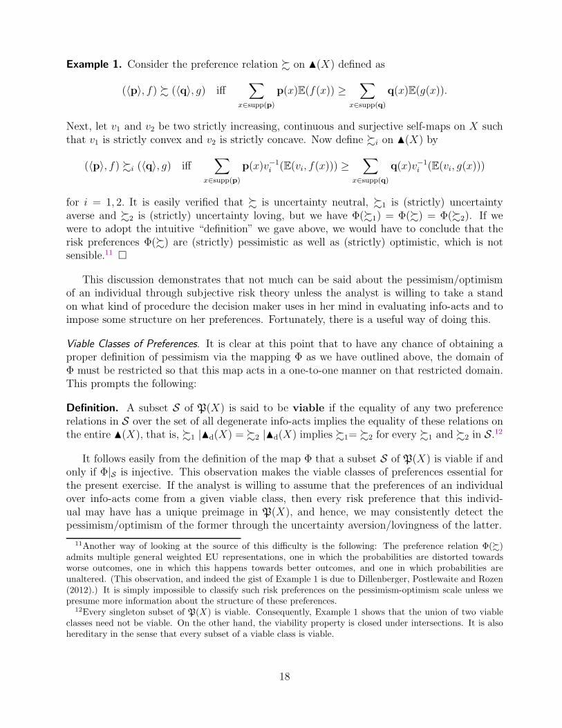
Example 1. Consider the preference relation ! on #(X) defined as

(⟨p⟩, f) ! (⟨q⟩, g) iff∑

x∈supp(p)

p(x)E(f(x)) ≥∑

x∈supp(q)

q(x)E(g(x)).

Next, let v1 and v2 be two strictly increasing, continuous and surjective self-maps on X suchthat v1 is strictly convex and v2 is strictly concave. Now define !i on #(X) by

(⟨p⟩, f) !i (⟨q⟩, g) iff∑

x∈supp(p)

p(x)v−1i (E(vi, f(x))) ≥

∑

x∈supp(q)

q(x)v−1i (E(vi, g(x)))

for i = 1, 2. It is easily verified that ! is uncertainty neutral, !1 is (strictly) uncertaintyaverse and !2 is (strictly) uncertainty loving, but we have Φ(!1) = Φ(!) = Φ(!2). If wewere to adopt the intuitive “definition” we gave above, we would have to conclude that therisk preferences Φ(!) are (strictly) pessimistic as well as (strictly) optimistic, which is notsensible.11 &

This discussion demonstrates that not much can be said about the pessimism/optimismof an individual through subjective risk theory unless the analyst is willing to take a standon what kind of procedure the decision maker uses in her mind in evaluating info-acts and toimpose some structure on her preferences. Fortunately, there is a useful way of doing this.

Viable Classes of Preferences. It is clear at this point that to have any chance of obtaining aproper definition of pessimism via the mapping Φ as we have outlined above, the domain ofΦ must be restricted so that this map acts in a one-to-one manner on that restricted domain.This prompts the following:

Definition. A subset S of P(X) is said to be viable if the equality of any two preferencerelations in S over the set of all degenerate info-acts implies the equality of these relations onthe entire #(X), that is, !1 |#d(X) = !2 |#d(X) implies !1= !2 for every !1 and !2 in S.12

It follows easily from the definition of the map Φ that a subset S of P(X) is viable if andonly if Φ|S is injective. This observation makes the viable classes of preferences essential forthe present exercise. If the analyst is willing to assume that the preferences of an individualover info-acts come from a given viable class, then every risk preference that this individ-ual may have has a unique preimage in P(X), and hence, we may consistently detect thepessimism/optimism of the former through the uncertainty aversion/lovingness of the latter.

11Another way of looking at the source of this difficulty is the following: The preference relation Φ(!)admits multiple general weighted EU representations, one in which the probabilities are distorted towardsworse outcomes, one in which this happens towards better outcomes, and one in which probabilities areunaltered. (This observation, and indeed the gist of Example 1 is due to Dillenberger, Postlewaite and Rozen(2012).) It is simply impossible to classify such risk preferences on the pessimism-optimism scale unless wepresume more information about the structure of these preferences.

12Every singleton subset of P(X) is viable. Consequently, Example 1 shows that the union of two viableclasses need not be viable. On the other hand, the viability property is closed under intersections. It is alsohereditary in the sense that every subset of a viable class is viable.

18

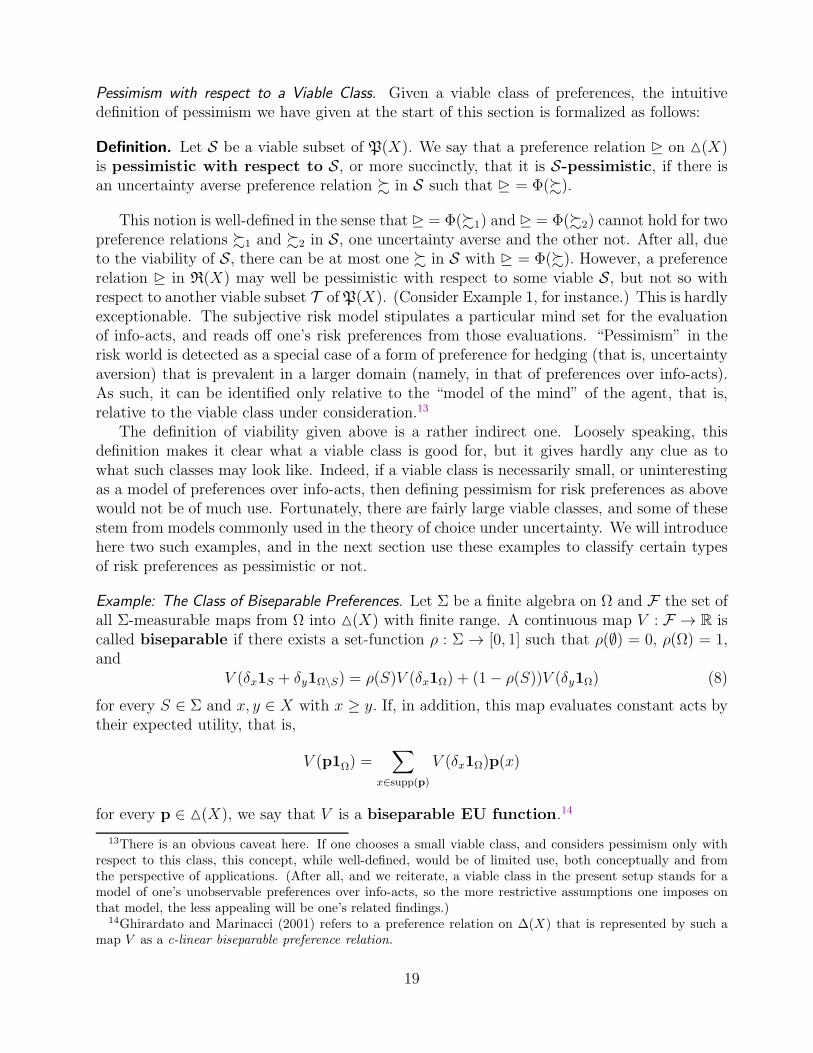
Pessimism with respect to a Viable Class. Given a viable class of preferences, the intuitivedefinition of pessimism we have given at the start of this section is formalized as follows:

Definition. Let S be a viable subset of P(X). We say that a preference relation $ on (X)is pessimistic with respect to S, or more succinctly, that it is S-pessimistic, if there isan uncertainty averse preference relation ! in S such that $ = Φ(!).

This notion is well-defined in the sense that $ = Φ(!1) and $ = Φ(!2) cannot hold for twopreference relations !1 and !2 in S, one uncertainty averse and the other not. After all, dueto the viability of S, there can be at most one ! in S with $ = Φ(!). However, a preferencerelation $ in R(X) may well be pessimistic with respect to some viable S, but not so withrespect to another viable subset T ofP(X). (Consider Example 1, for instance.) This is hardlyexceptionable. The subjective risk model stipulates a particular mind set for the evaluationof info-acts, and reads off one’s risk preferences from those evaluations. “Pessimism” in therisk world is detected as a special case of a form of preference for hedging (that is, uncertaintyaversion) that is prevalent in a larger domain (namely, in that of preferences over info-acts).As such, it can be identified only relative to the “model of the mind” of the agent, that is,relative to the viable class under consideration.13

The definition of viability given above is a rather indirect one. Loosely speaking, thisdefinition makes it clear what a viable class is good for, but it gives hardly any clue as towhat such classes may look like. Indeed, if a viable class is necessarily small, or uninterestingas a model of preferences over info-acts, then defining pessimism for risk preferences as abovewould not be of much use. Fortunately, there are fairly large viable classes, and some of thesestem from models commonly used in the theory of choice under uncertainty. We will introducehere two such examples, and in the next section use these examples to classify certain typesof risk preferences as pessimistic or not.

Example: The Class of Biseparable Preferences. Let Σ be a finite algebra on Ω and F the set ofall Σ-measurable maps from Ω into (X) with finite range. A continuous map V : F → R iscalled biseparable if there exists a set-function ρ : Σ → [0, 1] such that ρ(∅) = 0, ρ(Ω) = 1,and

V (δx1S + δy1Ω\S) = ρ(S)V (δx1Ω) + (1− ρ(S))V (δy1Ω) (8)

for every S ∈ Σ and x, y ∈ X with x ≥ y. If, in addition, this map evaluates constant acts bytheir expected utility, that is,

V (p1Ω) =∑

x∈supp(p)

V (δx1Ω)p(x)

for every p ∈ (X), we say that V is a biseparable EU function.14

13There is an obvious caveat here. If one chooses a small viable class, and considers pessimism only withrespect to this class, this concept, while well-defined, would be of limited use, both conceptually and fromthe perspective of applications. (After all, and we reiterate, a viable class in the present setup stands for amodel of one’s unobservable preferences over info-acts, so the more restrictive assumptions one imposes onthat model, the less appealing will be one’s related findings.)

14Ghirardato and Marinacci (2001) refers to a preference relation on ∆(X) that is represented by such amap V as a c-linear biseparable preference relation.

19

Recall that a preference relation ! on F is said to be monotonic if f ! g holds for everyf, g ∈ F such that f(ω)1Ω ! g(ω)1Ω for each ω ∈ Ω. Combining these two notions, we saythat a preference relation ! on F has a biseparable EU representation (or that it is abiseparable EU preference) if ! is monotonic, it deems more money preferable to less(that is, δx1Ω ! δy1Ω iff x ≥ y), and it can be represented by a biseparable EU function.

The class of preferences with biseparable EU representations were introduced by Ghi-rardato and Marinacci (2001, 2002). Roughly speaking, this class consists of those monotonepreferences that evaluate those acts that yield the same (objective) lottery at all states, andthose comonotonic acts with only two different (certain) outcomes according to the Anscombe-Aumann expected utility theory. This class is quite rich. It contains a variety of preferences,including preferences that correspond to the subjective expected utility (SEU), Choquet ex-pected utility (CEU), maxmin expected utility (MMEU), as well as preferences of Hurwicztype. Furthermore, it is straightforward to extend this notion to the case of preferences overinfo-acts: A preference relation ! in P(X) is said to be a biseparable EU preference if !p

has a biseparable EU representation for every p ∈ (X). The importance of such preferencesfor the present exercise stems from the following fact:

Proposition 3. Any collection of biseparable EU preference relations on #(X) is viable.15

In other words, the map Φ from P(X) into R(X) is injective on the class of all biseparableEU preferences on #(X). Therefore, this map is left-invertible on this class, that is, providedthat one’s preferences over info-acts are of biseparable EU type, we can identify these prefer-ences by observing the choices of this individual over monetary lotteries. We will demonstratein the next section that a good deal follows from this observation.16

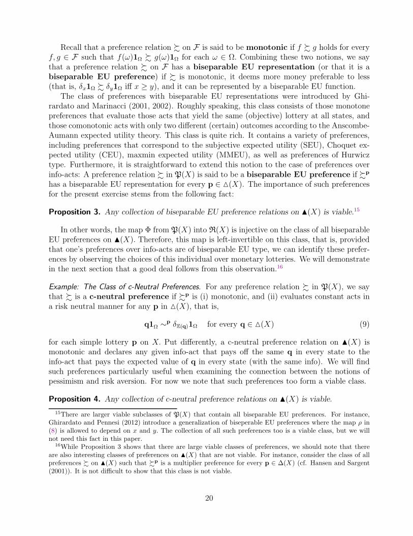
Example: The Class of c-Neutral Preferences. For any preference relation ! in P(X), we saythat ! is a c-neutral preference if !p is (i) monotonic, and (ii) evaluates constant acts ina risk neutral manner for any p in (X), that is,

q1Ω ∼p δE(q)1Ω for every q ∈ (X) (9)

for each simple lottery p on X. Put differently, a c-neutral preference relation on #(X) ismonotonic and declares any given info-act that pays off the same q in every state to theinfo-act that pays the expected value of q in every state (with the same info). We will findsuch preferences particularly useful when examining the connection between the notions ofpessimism and risk aversion. For now we note that such preferences too form a viable class.

Proposition 4. Any collection of c-neutral preference relations on #(X) is viable.

15There are larger viable subclasses of P(X) that contain all biseparable EU preferences. For instance,Ghirardato and Pennesi (2012) introduce a generalization of biseperable EU preferences where the map ρ in(8) is allowed to depend on x and y. The collection of all such preferences too is a viable class, but we willnot need this fact in this paper.

16While Proposition 3 shows that there are large viable classes of preferences, we should note that thereare also interesting classes of preferences on #(X) that are not viable. For instance, consider the class of allpreferences ! on #(X) such that !p is a multiplier preference for every p ∈ ∆(X) (cf. Hansen and Sargent(2001)). It is not difficult to show that this class is not viable.

20

Clearly, a c-neutral preference relation need not be of the biseparable EU form, nor is abiseparable EU preference necessarily c-neutral. As such, Propositions 3 and 4 are logicallydistinct. However, unlike the former, Proposition 4 is fairly straightforward. Indeed, if ! is ac-neutral preference in P(X), then f(x)1Ω ∼p δE(f(x))1Ω, and thus, by monotonicity,

f ∼p∑

x∈supp(p)

δE(f(x))1Ω(p,x).

for every (⟨p⟩, f) ∈ #(X). This means that such a preference relation is determined entirelyon the basis of its behavior on #d(X), and hence Proposition 4.

4.2 Applications

This section is devoted to the analysis of three concrete classes of risk preferences. Ourobjective is to characterize when a preference relation that belongs to any one of these classeswould be viewed as pessimistic (or optimistic) with respect to a particular viable class.

4.2.1 The Rank-Dependent Utility Model

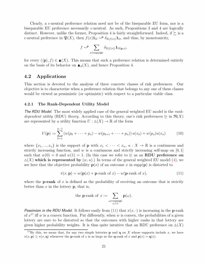
The RDU Model. The most widely applied case of the general weighted EU model is the rank-dependent utility (RDU) theory. According to this theory, one’s risk preferences $ in R(X)are represented by a utility function U : (X) → R of the form

U(p) :=n−1∑

k=1

(w(pk + · · ·+ pn)− w(pk+1 + · · ·+ pn)) u(xk) + w(pn)u(xn) (10)

where x1, ..., xn is the support of p with x1 < · · · < xn, u : X → R is a continuous andstrictly increasing function, and w is a continuous and strictly increasing self-map on [0, 1]such that w(0) = 0 and w(1) = 1. (In this case we refer to $ as an RDU preference on(X) which is represented by (w, u).) In terms of the general weighted EU model (4), wesee here that the objective probability p(x) of an outcome x in supp(p) is distorted to

π(x,p) = w(p(x) + p-rank of x)− w(p-rank of x), (11)

where the p-rank of x is defined as the probability of receiving an outcome that is strictlybetter than x in the lottery p, that is,

the p-rank of x :=∑

ω∈supp(p)ω>x

p(ω).

Pessimism in the RDU Model. It follows easily from (11) that π(x, ·) is increasing in the p-rankof x17 iff w is a convex function. Put differently, when w is convex, the probabilities of a givenlottery are sure to be distorted so that the outcomes with higher ranks in that lottery aregiven higher probability weights. It is thus quite intuitive that an RDU preference on (X)

17By this, we mean that, for any two simple lotteries p and q on X whose supports include x, we haveπ(x,p) ≥ π(x,q) whenever the p-rank of x is as large as the q-rank of x and p(x) = q(x).

21

which is represented by (w, u) would be deemed “pessimistic” if w is convex, and indeed, thisis precisely how pessimism is defined in the literature within the RDU model.

The RDUmodel provides a nice check for the appeal of our definition of pessimism. Indeed,within this domain, it seems quite clear how pessimism should be captured, and a definitionthat strays away from this would be suspect. Fortunately, in the context of the entire classof biseparable EU preferences on #(X) – recall Proposition 3 – our definition of pessimismmatches that defined for RDU preferences exactly.

Proposition 5. Let S stand for the class of all biseparable EU preference relations on #(X),and let $ be an RDU preference relation on (X) which is represented by (w, u). Then,$= Φ(!) for some ! in S. Furthermore, $ is S-pessimistic if, and only if, w is a convexfunction.

We are thus able to conform with the intuition derived within the RDU framework aboutpessimism through the foundations provided by preferences over info-acts (so long as thosepreferences are of the biseparable EU form).

4.2.2 The Multi-RDU Model

In a recent paper, Dean and Ortoleva (2013) have investigated risk preferences $ in R(X)that are represented by a utility function U : (X) → R of the form

U(p) := minw∈W

(

n−1∑

k=1

(w(pk + · · ·+ pn)− w(pk+1 + · · ·+ pn)) u(xk) + w(pn)u(xn)

)

(12)

where x1, ..., xn is the support of p with x1 < · · · < xn, u : X → R is a continuous andstrictly increasing function, and W is a nonempty convex set of continuous, strictly increasingand convex self-maps on [0, 1] that admit 0 and 1 as fixed points. A fairly straightforwardconsequence of Proposition 5 is that any such a preference relation is pessimistic with respectto the viable class S of biseparable EU preference relations on #(X).

There is, however, a more intimate connection between the work of Dean and Ortoleva(2013) and our approach toward modeling pessimism. That paper provides an axiomaticcharacterization of the above class of preferences, and one of its key axioms, called “Hedgingaxiom,” is primed to capture the potential pessimism of a decision-maker. This propertyutilizes outcome-mixtures in the style of Ghirardato et al. (2003) to formulate the notion ofhedging in the context of lotteries, and roughly speaking, says that a pessimistic person isone that exhibits preferences for hedging because this reduces the variance of utility-outcomes.While it is formally distinct from the way we have defined pessimism above, it is clear that themotivation behind the Dean-Ortoleva formulation of pessimism is similar to that behind ourapproach. In fact, it turns out that there is a formal connection between the two formulationsas well. Let $ be a preference relation in R(X) such that $ = Φ(!) for some ! in S.Then, one can show that $ is S-pessimistic iff it satisfies the Hedging axiom.18 Thus, the

18As this is mostly a side remark, we omit the proof of this fact here. It is, however, available from theauthors upon request.

22

two approaches to modeling pessimism are in sync, at least in the context of biseparable EUpreference relations.19

4.2.3 Disappointment Aversion and Pessimism

Gul’s Model. We consider next another important special case of the general weighted EUmodel, namely, Gul’s 1991 model of risk preferences that allows for disappointment aversionor elation loving. This model is described as follows. Take a risk preference $ in R(X), andfor any p ∈ (X), define

B(p,$) = q ∈ (X) : δx $ p for all x ∈ supp(q)

andW (p,$) = r ∈ (X) : p $ δx for all x ∈ supp(r).

A triplet (α,q, r) is said to be an elation/disappointment decomposition of p ∈ (X)with respect to $ if 0 ≤ α ≤ 1, q ∈ B(p,$), r ∈ W (p,$) and p = αq + (1 − α)r. (Ifthe certainty equivalent of p belongs to its support, there would be (infinitely) many suchdecompositions.)

We say that a $ ∈ R(X) is a Gul preference if it can be represented by a utility functionU : (X) → R of the form

U(p) = γ(α)∑

x∈supp(q)

q(x)u(x) + (1− γ(α))∑

x∈supp(r)

r(x)u(x), (13)

where (α,q, r) is an elation/disappointment decomposition of p with respect to $, u : X → R

is a continuous and strictly increasing function, and γ is a real map on [0, 1] such that

γ(t) =t

1 + (1− t)β, 0 ≤ t ≤ 1,

for some real number β > −1. (In this case we refer to $ as a Gul preference on (X)which is represented by (β, u).) Such a preference relation is said to be disappointmentaverse if β ≥ 0, and elation loving if −1 < β ≤ 0. It collapses to a standard expectedutility preference when β = 0.

Pessimism in Gul’s Model. Intuitively speaking, the construction of Gul’s preferences is basedon decomposing the support of a lottery into “good” outcomes and “bad” outcomes, andassigning different weights into these in the ensuing expected utility computation. Besides, itis clear that the higher β, the lower the γ (everywhere on its domain), and the more weightis assigned to “bad” outcomes in this representation. As β = 0 corresponds to the case ofexpected utility preferences, it is thus natural to view the case β > 0 as corresponding to the

19The link between the two approaches are broken when we go outside the biseparable EU preferencerelations. Put differently, if $ = Φ(!) does not hold for any ! in S, then the said equivalence fails. Perhapsmore important is the fact that, without this assumption (which roughly means the failure of the tradeoff-consistency axiom of Dean and Ortoleva (2013)), the Hedging axiom loses much of its appeal (as it becomesincompatible with outcome-mixtures other than the 50-50 ones).

23

case of pessimism. That is, it seems quite reasonable to call pessimism to what Gul refers toas disappointment aversion, and similarly, identify elation loving with optimism. As it turnsout, the definition of pessimism we introduced above (and again with respect to the viableclass of biseparable EU preferences) does precisely this.

Proposition 6. Let S stand for the class of all biseparable EU preference relations on #(X),and let $ be a Gul preference relation on (X) which is represented by (β, u). Then, $= Φ(!) for some ! in S. Furthermore, $ is S-pessimistic if, and only if, β ≥ 0.

Gul’s model thus provides another instance of the general weighted EU theory in which thepessimism notion we advance here turns out to yield the “correct” answer. This notion (withrespect to the viable class used above) coincides in this model with disappointment aversion.We will see in Section 4.3 that this would not at all be the case if we tried to define pessimismfor this model through probability distortions as in the case of the RDU model.

4.2.4 The Cautious Expected Utility Model

In the previous two examples we have dealt with two models of risk preferences relative towhich one has a strong feeling for what “pessimism” means. Our approach toward modelingpessimism thus conforms with intuition in the context of these examples. In our final applica-tion, we look at a type of risk preference relative to which it is not intuitively clear how one’spessimism could be captured.

Cautious Expected Utility. The cautious expected utility theory is developed in the recent workof Cerreia-Vioglio, Dillenberger and Ortoleva (2013). This theory provides an insightful ax-iomatic characterization for those preference relations $ ∈ R(X) which can be representedby a utility function U : (X) → R of the form

U(p) := infv∈V

v−1(E(v,p)), (14)

where V is a nonempty set of continuous and strictly increasing real maps on X such that (i)v(minX) = 0 = 1− v(maxX) for every v ∈ V, and (ii) U is continuous. Given such a $ andV, we say that $ is a cautious EU preference on (X) which is represented by V, orequivalently, that V is a cautious EU representation for $.

Not every such preference arises through Φ by a biseparable EU preference on info-acts,so examining the pessimism properties of cautious EU preferences requires using a differentviable class. It is easily seen that the class of c-neutral preferences can be used for this purpose.Indeed, take any cautious EU preference $ on (X) which is represented by V, and considerthe map U∗ : #(X) → R defined by

U∗(⟨p⟩, f) := infv∈V

v−1

⎛

⎝

∑

x∈supp(p)

p(x)v(E(f(x)))

⎞

⎠ . (15)

It is easy to see that$ = Φ(!) where ! is the preference relation on #(X) which is representedby U∗. Besides, it is also routine to verify that ! belongs to P(X) and is c-neutral. We may

24

thus conclude that every cautious EU preference relation in R(X) is the image of some c-neutral preference relation in P(X) under Φ. As the collection of all c-neutral preferencesin P(X) is viable (Proposition 4), it is meaningful to classify cautious EU preference on thebasis of pessimism relative to the class of c-neutral preferences on #(X). This leads us to aninteresting observation:

Proposition 7. Let S stand for the class of all c-neutral preference relations on #(X), andlet $ be a cautious EU preference on (X) which is represented by V . Then, $ = Φ(!) forsome ! in S. Furthermore, $ is S-pessimistic if, and only if, it is risk averse.

In the context of the cautious EU model, we thus find that the notion of pessimism (withrespect to the class of c-neutral preference relations) reduces to the standard property of riskaversion.

Remark. In passing, we note that it is also possible to characterize the pessimism of $functionally in the context of Proposition 7. Indeed, if every v in V is concave, then $ is riskaverse, and hence, S-pessimistic. Conversely, if $ is S-pessimistic, then there is a subset Wof V such that W is a cautious EU representation for $ and every element of W is concave.20

4.3 The General Weighted EU Model and Pessimism

Intuitively, an individual is considered “pessimistic” in the literature if she distorts the proba-bility of outcomes in such a way that she views low outcomes as more likely than they actuallyare. As such, this notion is defined in the literature only for some special cases of the generalweighted EU model. To be precise, let us consider a preference relation $ in R(X) that canbe represented by a utility function U : (X) → R of the form (4) where u : X → R isa continuous and strictly increasing function and π a probability weighting function on X.Given that we interpret π(x,p) as the distorted probability of receiving x in the lottery, itseems reasonable to define “pessimism” by suitably comparing the distorted probabilities withthe original ones (in the case of all lotteries).

Recall that, for any p ∈ (X) and x ∈ supp(p), the p-rank of x is the probability ofreceiving an outcome that is strictly better than x in the lottery p. This concept allows us tounderstand how good x is relative to the other outcomes in the support of p. The higher thep-rank order of x, the worse this outcome is relative to these other outcomes. This promptsthe following formulation which is commonly adopted in the literature:

Definition. Let $ be a general weighted EU preference on (X) which is represented by(π, u). We say that $ is π-pessimistic if for any p and q in (X), and any x that belongs tothe supports of both p and q, we have π(x,p) ≥ π(x,q) whenever the p-rank of x is as largeas the q-rank of x and p(x) = q(x). (We define π-optimism dually.)

Unfortunately, there are some difficulties with this definition. First of all, defining pes-simism through the probability weighting function used in a representation of the form (4)

20The latter statement obtains by combining Theorem 3 of Cerreia-Vioglio, Dillenberger and Ortoleva (2013)with our Proposition 7. Loosely speaking, the reason why we need to consider a subset of V instead of theentire V is because this set may include functions that are redundant for the computation of the utility functiongiven in (14).

25

is, in general, behaviorally untenable. This is because π and u are not uniquely determinedin the representation (4). It is not difficult to find two pairs (π, u) and (π′, u′) that repre-sent the same preference relation on (X) such that this preference relation is π-pessimisticbut not π′-pessimistic. Put differently, in the general weighted EU model, the definition ofπ-pessimism does not depend only on $ for which we have a representation by (π, u).

This difficulty is well known. In response, most authors adopt the definition of pessimismabove in certain special cases of the general weighted EUmodel in which π is uniquely identified(and u is determined up to positive affine transformations). Obviously, this is not unrelatedto why we had to introduce the notion of a viable class above. However, the nature of thedependence of our formulation of pessimism on the choice of the viable class is different thanhow “π-pessimism” concept depends on the class of general weighted EU preferences. First,the former definition is behaviorally meaningful, while, as we have noted above, the latter is notso in general. Second, a viable class is not necessarily characterized by a particular functionalform, but rather by means of either structural or behavioral properties. For instance, we haveseen earlier that the collection of all biseparable EU preferences, as well as that of all c-neutralpreferences, on #(X) are viable, but these classes are not characterized by functional formspecifications. (The former is determined by structural properties, while the latter purelybehavioral properties.) Finally, and more importantly, by choosing different viable classes,one can trace entirely different types of risk preferences (by looking at the image of theseclasses under Φ). By varying the viable classes, therefore, the present definition of pessimismmodifies and becomes applicable to essentially any type of risk preferences.

Pessimism in the RDU Model, Revisited. In the representation (10) w is uniquely identified(and u is unique up to positive affine transformations). Put differently, within the RDUtheory, the probability weighting function π is uniquely defined by one’s preferences, and thusthe definition of π-pessimism is behaviorally meaningful. Furthermore, in that model, thisdefinition leads to a nice characterization: An individual whose preference relation on ∆(X)is an RDU preference which is represented by (w, u) is π-pessimistic (where π is defined by(11)) iff w is a convex function. (π-Optimism is captured dually.)21 In view of Proposition 5,therefore, we find that the notion of pessimism adopted in the literature for the RDU modelis in full accord with the way we have defined this concept (with respect to the viable class ofbiseparable preferences).

A natural query is if this observation extends to other subclasses of the general weighted EUtheory (in which the probability weighting functions are uniquely identified). Put differently,is it the case that the notion of pessimism we have introduced via the subjective risk modelis none other than how pessimism is defined in the context of general weighted EU theory(whenever the latter conceptualization of pessimism in terms of probability distortions isbehaviorally meaningful)? The answer is no, as we show next.

Pessimism in Gul’s Model, Revisited. Let $ be a Gul preference relation on (X) which isrepresented by (β, u). It can be shown that $ is of the general weighted EU form, that is,

21This observation is stressed, for instance, in Wakker (1994) and Abdellaoui (2002), among numerousother authors. It is common in the literature on RDU theory to take the convexity of w as the “definition” ofpessimism.

26

it can be represented by a utility function of the form (4) for some probability weightingfunction π and u. Unlike the RDU model, however, the utility function U that represents $as in Gul’s model is only implicitly defined, so we cannot in general provide a closed-formdescription of the map π in terms of β and u. However, as proved in Theorem 1 of Gul (1991),β is unique here and u is unique up to positive affine transformations, so π is in fact uniquelyidentified. Consequently, as in the RDU model, it is behaviorally meaningful to view $ aspessimistic when it is π-pessimistic. Unfortunately, in this case, this way of looking at thetrait of pessimism does not turn out to be useful:

Proposition 8. Let $ be a Gul preference relation on (X), and let this relation be repre-sented by (π, u) as in the general weighted EU model. Then, the following are equivalent: (i)$ is π-pessimistic; (ii) $ is an expected utility preference; (iii) $ is π-optimistic.

In words, an attempt to extend the rank-based definition of “pessimism” to Gul’s modelcannot classify any preferences in that model on the pessimism-optimism scale, with theexception of the standard expected utility preferences (which are neutral so far as that scale isconcerned). Looking at pessimism by means of probability weighting functions is simply toocoarse to declare an agent with Gul preferences as pessimistic in a nontrivial manner. Gul’smodel thus provides an instance of the general weighted EU theory in which the definition ofpessimism that is commonly adopted in the literature does not deliver an intuitive answer, butthe pessimism notion we advance here turns out to yield arguably the “correct” answer. As wehave found in Proposition 6, the latter notion (with respect to the viable class of biseparableEU preferences) coincides in this model with disappointment aversion.

Pessimism in the Cautious Expected Utility Model, Revisited. Let $ be a cautious EU preferenceon (X) which is represented by V. This preference too is of the general weighted EU form,so we may think of classifying it as pessimistic or not by using the π-pessimism notion.However, in this case, this notion is not even operational. For, as we have noted above, thisdefinition is meaningful only on subclasses of general weighted EU preferences in which theprobability weighting function is unique and the utility function is unique up to positive affinetransformations. So, to use the π-pessimism concept for the cautious expected utility model,we need to see this model as a subcollection of all general weighted EU preferences which isrepresented by (π, u) such that (π, u) satisfies some conditions (that ensure their uniqueness).This is exactly what we have done above with the RDU model and Gul’s model, but there wasa natural way of choosing the (π, u)s for the representations in those models, and hence, itwas clear which subcollections of the general weighted EU preferences are to be used. Insofaras we can see, this is not the case for the cautious EU model. There does not seem to bea natural way of viewing $ as represented in the general weighted EU form by means of aparticular pair (π, u) (and of course, there are infinitely many such pairs that are up to thetask). Put differently, the standard practice of limiting attention to a particular subclass ofgeneral weighted EU preferences and then applying the π-pessimism notion does not work(at least in a straightforward manner) in the context of the cautious EU theory. As we haveseen in Proposition 7, however, our formulation of pessimism (with respect to the viable classof c-neutral preferences) does not encounter such a difficulty, and classifies a cautious EUpreference as pessimistic iff it is risk averse.

27

5 Pessimism and Probabilistic Risk Aversion

Probabilistic Risk Aversion. In contrast to the classical expected utility theory under risk, thecharacterization of risk aversion is often a complicated matter in the context of non-expectedutility theories. For instance, in the case of a preference relation on ∆(X) that is representedby a utility function of the form (4) as in the generalized weighted EU model, attitudestoward risk arise both from the structure of the probability weighting function π (distortionof probabilities) and the curvature of u (utility for money). The former effect, that is, theinfluence of probability weighting on risk attitudes is referred to as probabilistic risk attitudein the literature. To understand this effect in isolation, one may take u as an affine functionin (4), and then characterize the risk attitudes of preferences in terms of the structure ofthe probability weighting function (provided that this function is uniquely determined). Forinstance, one can look for a functional characterization of the probability weighting functionsthat represent risk averse preferences when coupled with an affine utility function for money.Informally speaking, such a characterization would tell us when the agent can be viewed asprobabilistically risk averse, that is, when her probability distortions contribute positively toher potential risk aversion.22

In the subjective risk model, we obtain the distortions of objectively given probabilitiesfrom one’s preferences over info-acts. Consequently, we may ask what sort of behavioral traitsof the latter type of preferences would be responsible for inducing distortions of probabilitiesthat exhibit particular types of probabilistic risk attitudes. We shall investigate this query herein terms of probabilistic risk aversion. This investigation parallels the one we have reportedin Section 3. We have seen there that deviations from ambiguity neutrality (in terms ofpreferences over info-acts) is a necessary condition for the resulting risk preferences to divergefrom the expected utility model (and hence some distortion of objective probabilities to occur).We shall now attempt to identify what must be true for one’s preferences over info-acts sothat the induced risk preferences exhibit probabilistic risk aversion. Put succinctly, we wishto utilize the subjective risk theory to find a “source” for one’s probabilistic risk aversion.

Uncertainty Aversion implies Probabilistic Risk Aversion. To make things precise, let us recallthat a simple lottery q on X is a mean-preserving spread of another such lottery p if,where supp(p) is enumerated as x1, ..., xk, there exist simple lotteries θ1, ..., θk on X suchthat

q =k∑

i=1

p(xi)θi and E(θi) = xi for each i = 1, ..., k.

In turn, a preference relation $ on ∆(X) is said to be risk averse if p $ q for everyp,q ∈ ∆(X) such that q is a mean-preserving spread of p.23

Our objective here is to understand what sort of properties of a preference relation ! on#(X) entails the risk aversion of Φ(!) insofar as this arises due to one’s subjective assessmentof the likelihoods in a given lottery. Obviously, this issue is irrelevant for the comparative

22We stress that a probabilistically risk averse agent need not be risk averse in the final analysis. Theoverall attitude toward risk requires the joint input of both the probability weighting function and the utilityfunction.

23In the context of non-expected utility theory, what we define here as risk aversion is often referred to asstrong risk aversion.

28

evaluation of two constant info-acts (whose “info” parts are the same). Consequently, weshall impose that the preferences at hand act in a risk neutral manner when comparing suchinfo-acts, that is, we shall impose (9) on !. If ! satisfies this property, any risk aversion thatmay be detected in the induced risk preferences Φ(!) must arise from the way this personevaluates the uncertainty she perceives in a given lottery in terms of the likelihoods of prizes.Therefore, our problem may be stated as follows: For any c-neutral preference relation ! on#(X), when would Φ(!) be a risk averse preference relation on ∆(X)? We now show that asufficient condition for this is none other than uncertainty aversion.

Theorem 9. Let ! be a c-neutral preference relation on #(X). If ! is uncertainty averse,then Φ(!) is risk averse.

The subjective risk theory thus brings together two empirically meaningful phenomena,uncertainty aversion and risk aversion, that exist in formally disparate realms. Of course, wecan restate this connection by using only one’s risk preferences as a primitive:

Corollary 10. Let S be the class of all c-neutral preference relations on #(X). Then, everyS-pessimistic preference relation $ on ∆(X) is risk averse.

Informally speaking, therefore, we find that the general notion of pessimism we have in-troduced in this paper entails the probabilistic risk aversion of one’s risk preferences, at leastwhen pessimism is understood relative to the viable class of c-neutral preference relations.

An Open Problem. We have seen in Section 4.2.1 that an RDU preference $ on ∆(X) whichis represented by (w, u) is pessimistic with respect to the biseparable EU class S iff w isconvex. By Propositions 4 and 5, there is a unique biseparable EU preference ! on #(X)with $= Φ(!). Besides, it is readily checked that u is affine iff ! satisfies (9). Consequently,in the context of c-neutral and biseparable EU class, we find that $ is uncertainty averse iffw is convex. But it is well-known that $ is risk averse iff w is convex and u is concave (cf.Chew, Karni and Safra (1987)). It follows that the converse of Theorem 9 is valid, providedthat Φ(!) has an RDU representation. In fact, precisely the same is true when Φ(!) is aGul preference, and as we have already noted in Proposition 7, for the cautious EU model.These observations lead us to conjecture that the converse of Theorem 9 is true: A c-neutralpreference relation on #(X) is uncertainty averse if, and only if, the risk preference that itinduces is risk averse. If true, this statement would mean that one’s probabilistic risk aversionis but only a reflection of her uncertainty aversion. Finding whether or not the “if” part ofthis statement is true, however, is left as an open problem at present.

6 Pessimism and Preference for Diversification

Intuitively, we would expect a pessimistic individual to very much dislike “putting all eggs inone basket.” Instead, it seems reasonable that she would try to reduce the risk involved in herinvestments as much as possible by mixing her assets, thereby diversifying her portfolio, evenif her utility for money is a linear function. The definition of pessimism that is used in non-expected utility theory would be consistent with this intuition only in special cases. That is,

29

the π-pessimism of a general weighted EU preference on (X) which is represented by (π, u),where u is the identity function, may or may not result in a preference for diversification. Inparticular, this happens in the context of the RDU model but not in Gul’s model (Proposition8). By contrast, we show in this section that the notion of pessimism we have introduced here(with respect to c-neutral preferences over info-acts) is consistent with this intuition in fullgenerality.

Preferences over Assets. We adopt the model of Dekel (1989) to formalize the problem. Con-sider the standard probability space ([0, 1],B, ℓ), where B is the Borel σ-algebra on [0, 1] andℓ is the Lebesgue measure. For any random variable x from this space into X , we denote thesimple probability measure on X induced by x by px, that is, px := ℓ x−1. In what follows,by an asset on X, we mean such a random variable with a finite range. Obviously, for anyasset x on X, px is a simple lottery on X. Consequently, the preferences of a decision makerover assets on X are naturally induced by her preference relation $ on (X). It is convenientto abuse notation and denote the former preferences also by $ here. That is, for any twoassets x and y on X, by x $ y we mean simply that px $ py.

Pessimism implies Preference for Portfolio Diversification. We say that a preference relation $over assets on X exhibits preference for portfolio diversification if, for any positiveinteger n and assets x1, ..., xn on X,

x1 ≃ · · · ≃ xn implies λ1x1 + · · ·+ λnxn $ x1

for every λ1, ...,λn ≥ 0 with λ1 + · · · + λn = 1.24 Our final result in this paper is that ifa preference relation over assets on X arises from risk preferences that are pessimistic withrespect to the viable class of c-neutral preferences, then it must exhibit preference for portfoliodiversification.

Theorem 11. Let S be the class of all c-neutral preference relations on #(X). Then, everyS-pessimistic preference relation $ on ∆(X) exhibits preference for portfolio diversification.

In passing, we note that, unlike the case of Theorem 9, we do know that the converse ofTheorem 11 is false: Preference for diversification does not imply pessimism (with respect toc-neutral preferences). This is because the former concept imposes restrictions only on theinfo-acts that belong to the range of the canonical map ϕ. The info-acts that are not inducedby lotteries lie outside this range, and as a result, a risk preference that exhibits a preferencefor diversification need not be pessimistic (with respect to c-neutral preferences).

Remark. Dekel (1989) has shown that a continuous (first-order) stochastically increasingpreference relation over assets on X is risk averse, provided that it exhibits preference fordiversification. Combining this result with Theorem 11, therefore, yields an alternate prooffor our Theorem 9.

24Here ≃ denotes the symmetric (indifference) part of $.

30

7 Summary

The ultimate objective of this paper was to introduce a model of evaluating objectively givenlotteries in a subjective manner. We have done this by reformulating lotteries as “info-acts,”and presuming that a decision maker may view a lottery in her “mind” as such. This model,which we refer to as the subjective risk theory, allows the analyst to view one’s risk preferencesas arising from her preferences over info-acts, thereby relating attitudes toward uncertaintyto those toward risk. Our main theoretical finding was that if one is neutral to ambiguity (inher “mind”), then her risk preferences are bound to be of the classical expected utility form.Consequently, this model envisages that any deviation from the expected utility paradigm isto be attributed to one being not neutral toward the evaluation of uncertainty.

The second part of the paper has attempted to investigate the connection between one’sattitudes toward uncertainty and the structure of her risk preferences a bit more closely. Inparticular, we have explored the intuition that if one has a global preference for hedging (inher “mind”), which means that she is rather pessimistic in the evaluation of uncertainty atlarge, then her (observed) risk preferences must exhibit “pessimism.” We have taken this as adefinition of pessimism in the risk context (when it is formally possible to do so), and showedthat this definition not only matches that used in the literature in the context of RDU theory,but that it yields insights which are not possible to deduce from the latter formulation. Inparticular, we have shown that the notion of pessimism for risk preferences we introduce herereduces to disappointment aversion in the context of Gul’s model, while, in general, it impliesprobabilistic risk aversion as well as preference for diversification. These properties accordwell with what one would intuitively expect from the behavior of a “pessimistic person,” andhence provide support for the general formulation we advance here. In general, none of themwould be valid with respect to the definition of pessimism utilized in the previous literature.

31

PROOFS

Notation. For any p ∈ (X) and any map Ψ from supp(p) into a linear space, we shall adopt the followingnotation in the remainder of this paper:

∑

pΨ(x) :=

∑

x∈supp(p)

Ψ(x).

PROOF OF PROPOSITION 1

Lemma A.1. Let $ be a preference relation in R(X). Then, $ can be represented as in the general weightedEU model if, and only if,

δmax supp(p) $ p $ δmin supp(p) for every p ∈ (X). (16)

Proof. The “only if” part of the assertion is straightforward, so we focus only on its “if” part. Take any$ ∈ R(X) such that (16) holds. For any (fixed) r in (X), let x∗(r) and x∗(r) stand for the minimum andmaximum elements of the set supp(r), respectively, and define

A := λ ∈ [0, 1] : r $ δ(1−λ)x∗(r)+λx∗(r) and B := λ ∈ [0, 1] : δ(1−λ)x∗(r)+λx∗(r) $ r.

These sets are nonempty, for 0 ∈ A and 1 ∈ B by (16). On the other hand, both A and B are closed (because$ is continuous) while A ∪B = [0, 1] (because $ is complete). Since [0, 1] is connected, therefore, A ∩B = ∅.Conclusion: For every r ∈ (X) there is a λ(r) ∈ [0, 1] such that

r ≈ δ(1−λ(r))x∗(r)+λ(r)x∗(r),

where ≈ is the symmetric part of $. Now define U : (X) → R by

U(r) := (1− λ(r))x∗(r) + λ(r)x∗(r).

Notice that, for any r ∈ (X) we have U(r) =∑

rπ(x, r)x, where π(x∗(r), r) = 1 − λ(r), π(x∗(r), r) = λ(r),

and π(x, r) = 0 for any x in supp(r) distinct from x∗(r) and x∗(r). On the other hand, U represents $ .Indeed, for any p and q in (X), we have p $ q iff δU(p) $ δU(q) by definition of U, while the latter statementholds iff U(p) ≥ U(q) because money is a desirable commodity according to $. We conclude that $ admitsa general weighted EU representation. '

To prove Proposition 1, take any preference relation ! in P(X) and set $ := Φ(!). As we have verifiedin Section 2.3, $ belongs to R(X). In view of Lemma A.1, therefore, all we need to do is to verify (16) for $.To this end, fix an arbitrary p in (X) and let x∗ stand for the maximum element of supp(p). By definitionof the maps Φ,

δx∗ $ p iff (⟨δx∗⟩, δx∗1Ω) !(

⟨p⟩,∑

pδx1Ω(p,x)

)

iff (⟨p⟩, δx∗1Ω) !(

⟨p⟩,∑

pδx1Ω(p,x)

)

where we have invoked the State Invariance Axiom to obtain the second equivalence. Put differently, we haveδx∗ $ p iff δx∗1Ω !p fp, so, by the monotonicity hypothesis of Proposition 1, we may conclude that δx∗ $ p.As we can similarly verify that p $ δmin supp(p) as well, our proof is complete.

SOME PRELIMINARY LEMMATA

To prove the remaining theorems, we will make use of the following preliminary results whose statements makeuse of the following bit of notation:

Notation. For any lottery p ∈ (X) and any nonempty subset C of supp(p), we define

Ω(p, C) :=⋃

x∈C

Ω(p, x),

32

that is, Ω(p, C) is the event in Ω in which p takes value within C.

Lemma A.2. Let ! be a monotonic preference relation in P(X) such that

(⟨p⟩, f) ! (⟨p⟩, g) implies (⟨p⟩,αf + (1− α)g) ! (⟨p⟩, g) (17)

for every p ∈ (X), f, g ∈ F(p) and 0 < α < 1. Then, for any (⟨p⟩, f) ∈ #(X) and nonempty subset C ofsupp(p), we have

(⟨p⟩, r1Ω(p,C) + f1Ω\Ω(p,C)) ! (⟨p⟩, f), (18)

where

r :=∑

x∈C

p(x)

p(C)f(x).

Proof. In view of the continuity of !, it is enough to establish the lemma for p ∈ (X) that takes rationalvalues. Fix then some p ∈ (X) with p(x) ∈ Q for each x ∈ supp(p). Let C be a nonempty subset of supp(p).If C is a singleton, there is nothing to prove, so we assume |C| ≥ 2. Our proof is by induction on the size of|C| .

Let us first consider the case |C| = 2, so put C = x′, x′′ for some distinct x′, x′′ ∈ supp(p). As p isrational-valued, there are two positive integers (with no common divisors) m and n such that

p(x′)

p(x′) + p(x′′)=

m

n.

(Obviously, m < n.) Now pick any real numbers x0, ..., xn−1 in X\supp(p) and set

S := x0, ..., xn−1 and Si := xi, ..., x(i+m−1)modn, i = 0, ..., n− 1.

We define q ∈ (X) by

q =n−1∑

i=0

1np(C)δxi +

∑

x∈supp(p)\C

p(x)δx.

(Note that supp(q) = S ∪ (supp(p)\C) and q(S) = p(C).) Next, for each i = 0, ..., n− 1, put

gi := f(x′)1Ω(q,Si) + f(x′′)1Ω(q,S\Si) + f1Ω(q,supp(p)\C)

which belongs to F(q). As q(Si) = p(x′) and q(S\Si) = p(x′′) for each i = 0, ..., n − 1, we may invoke theState Invariance Axiom to find

(⟨p⟩, f) ∼ (⟨q⟩, gi) for each i = 0, ..., n− 1. (19)

Now set

g :=n−1∑

i=0

1ngi,

and note that g ∈ F(q) and g =(

mn f(x′) + n−m

n f(x′′))

1Ω(q,S) + f1Ω\Ω(q,S). As Ω(q, S) = Ω(p, C), definingr as in the statement of the lemma allows to write g = r1Ω(p,C)+ f1Ω\Ω(p,C). Clearly, by the State InvarianceAxiom, we have

(⟨q⟩, g) ∼ (⟨p⟩, r1Ω(p,C) + f1Ω\Ω(p,C)). (20)

But as (⟨q⟩, g0) ∼ · · · ∼ (⟨q⟩, gn−1) by (19), applying the hypothesis (17) inductively yields

(⟨q⟩, g) ! (⟨q⟩, gi) for each i = 0, ..., n− 1.

Combining this observation with (19) and (20) establishes (18).As the induction hypothesis, we now assume that our claim is valid for any fixed integer 2 ≤ k < |supp(p)|

and nonempty subset C of supp(p) with |C| ≤ k. To complete the proof, take any C ⊆ supp(p) with |C| = k+1,say, C = x0, ..., xk for some distinct x0, ..., xk ∈ supp(p). We define q ∈ (X) by

q(x) :=

p(x), if x = x0 or x ∈ supp(p)\Cp(C\x0), if x = x1.

33

(Note that p(C) = qx0, x1 and p(x0) = q(x0).) Next, we put

r′ :=k∑

i=1

p(xi)

p(C\x0)f(xi),

and note that

r =p(x0)

p(C)f(x0) +

p(C\x0)

p(C)r′,

where r is as defined in the statement of the present lemma. Then, first by applying the State InvarianceAxiom and then what we have found in the previous paragraph (where q plays the role of p and x0, x1 thatof C), we find

(⟨p⟩, r1Ω(p,C) + f1Ω\Ω(p,C)) ∼ (⟨q⟩, r1Ω(q,x0,x1) + f1Ω\Ω(q,x0,x1))

! (⟨q⟩, f(x0)1Ω(q,x0) + r′1Ω(q,x1) + f1Ω\Ω(q,x0,x1)).

On the other hand, applying the State Invariance Axiom, and then the induction hypothesis (with C\x0playing the role of C) yield

(⟨q⟩, f(x0)1Ω(q,x0) + r′1Ω(q,x1) + f1Ω\Ω(q,x0,x1)) ∼ (⟨p⟩, f(x0)1Ω(p,x0) + r′1Ω(p,C\x0) + f1Ω\Ω(p,C))

! (⟨p⟩, f).

Combining these two findings, we get (⟨p⟩, r1Ω(p,C) + f1Ω\Ω(p,C)) ! (⟨p⟩, f), and our proof is complete.

The proof above modifies trivially to show that if (17) is replaced with

(⟨p⟩, f) ! (⟨p⟩, g) implies (⟨p⟩, f) ! (⟨p⟩,αf + (1− α)g)

in the statement of Lemma A.2, then (18) would modify to

(⟨p⟩, f) ! (⟨p⟩, f1Ω\Ω(p,C) + r1Ω(p,C)).

Consequently, setting C = supp(p) in Lemma A.2, adopting the notation

p⊙ f :=∑

x∈supp(p)

p(x)f(x) for any (⟨p⟩, f) ∈ #(X),

and using this “dual” observation, we get:

Corollary A.3. Let ! be a monotonic preference relation in P(X) such that (17) holds for every p ∈ (X),f, g ∈ F(p) and 0 < α < 1. Then,

(⟨p⟩, (p⊙ f)1Ω) ! (⟨p⟩, f) (21)

for each (⟨p⟩, f) ∈ #(X). Moreover, if

(⟨p⟩, f) ∼ (⟨p⟩, g) implies (⟨p⟩,αf + (1− α)g) ∼ (⟨p⟩, f), (22)

for every p ∈ (X), f, g ∈ F(p) and 0 < α < 1, then ∼ holds in (21).

PROOF OF THEOREM 2

Lemma A.4. Let ! be a monotonic and ambiguity neutral preference relation in P(X). Then, there is acontinuous and strictly increasing function u : X → R, and for each p ∈ (X), there is a probability measureµp on the algebra generated by Ω(p) such that

(⟨p⟩, f) ! (⟨p⟩, g) iff∑

pµp(Ω(p, x))E(u, f(x)) ≥

∑

pµp(Ω(p, x))E(u, g(x)), (23)

for every f, g ∈ F(p).

34

Proof. Ambiguity neutrality of ! means that, for every p ∈ (X), there exist two preference relations !p

0and !p

1 on F(p) such that(i) there is a map up : X → R and a probability measure µp on the algebra generated by Ω(p) such that

the map Vp : F(p) → R, defined by

Vp(f) :=∑

pµp(Ω(p, x))E(up, f(x)),

represents !p

0 ;(ii) there is a map u′

p: X → R and a probability measure µ′

pon the algebra generated by Ω(p) such that

the map Vp : F(p) → R, defined by

Vp(f) :=∑

pµ′p(Ω(p, x))E(u′

p, f(x)),

represents !p

1 ;(iii) r1Ω !p

1 g implies r1Ω !p g and r1Ω !p g implies r1Ω !p

0 g for each r ∈ (X) and g ∈ F(p).As implied by Theorem 17 of Ghirardato and Marinacci (2002), it must be that u′

pis a positive affine trans-

formation of up, and µ′p = µp for each p ∈ (X), meaning that !p

1 coincides with !p

0 for each p ∈ (X).From (i) we see that r1Ω !p

0 r′1Ω iff E(up, r) ≥ E(up, r′) for every r, r′ ∈ (X) and p ∈ (X). Onthe other hand, by the State Invariance Axiom, r1Ω !p

0 r′1Ω iff r1Ω !q

0 r′1Ω, for every r, r′ ∈ (X) andp,q ∈ (X). It follows that we may take up to be independent of p in the representation of !p

0 . (We thuswrite u for up in what follows.) In turn, (iii) implies that δx1Ω !p δy1Ω iff u(x) ≥ u(y) for every x, y ∈ X ,so, as ! satisfies the desirability of money, we see that u must be strictly increasing. On the other hand, forany given p, if we define the preference relation $ on (X) by r $ r′ iff r1Ω !p r′1Ω, (i) and (iii) entail thatu is a von Neumann-Morgenstern utility function for $. Thus $ satisfies the standard Independence Axiom.Besides, as !p is continuous, $ is continuous as well. But then, $ admits an expected utility representationwith a continuous von Neumann-Morgenstern utility function, and of course, u must then be a positive affinetransformation of that function. It follows that u is continuous.

Now fix any p ∈ (X), and take any f and g in F(p). Given that !p

0 admits an expected utilityrepresentation in the standard sense, there exists a lottery r in (X) such that f ∼p

0 r1Ω. By (iii), then,r1Ω !p f . To derive a contradiction, suppose r1Ω ≻p f . Then, by monotonicity of !p, there must be an x ∈supp(p) such that r1Ω ≻p f(x)1Ω. In turn, by continuity of !p, we can find a (large enough) λ in (0, 1) withr1Ω ≻p (λr + (1 − λ)f(x))1Ω ≻p f . But then, by (iii), we find r1Ω ≻p

0 (λr + (1 − λ)f(x))1Ω !p

0 f , that is,r1Ω ≻p

0 f , a contradiction. Conclusion: f ∼p r1Ω. Consequently, using (iii) again,

f !p

0 g iff r1Ω !p

0 g iff r1Ω !p g iff f !p g.

Combining this with (i), and recalling that up does not depend on p, completes the proof.

To prove Theorem 2, let ! be a monotonic and ambiguity neutral element of P(X), and find u : X → R

and µp (for each p in (X)) as in Lemma A.4. Note in particular that, for any p ∈ (X),

r1Ω !p r′1Ω iff E(u, r) ≥ E(u, r′) (24)

for every r, r′ ∈ (X). Another consequence of the representation (23) is that, for any p ∈ (X), the preferencerelation !p on F(p) satisfies (22), and hence, by Corollary A.3,

(⟨p⟩, f) ∼ (⟨p⟩, (p⊙ f)1Ω) for every f ∈ F(p).

But then, for any (⟨p⟩, f) and (⟨q⟩, g) in #(X), we have (⟨p⟩, f) ! (⟨q⟩, g) iff

(⟨p⟩, (p⊙ f)1Ω) ! (⟨q⟩, (q⊙ g)1Ω) ,

which, by the State Invariance Axiom, holds iff

(⟨p⟩, (p⊙ f)1Ω) ! (⟨p⟩, (q⊙ g)1Ω) ,

35

which, in view of (24), holds iff E(u,p⊙ f) ≥ E(u,q⊙ g), that is,

∑

pp(x)E(u, f(x)) ≥

∑

pq(x)E(u, g(x)).

It follows that, for any p,q ∈ (X), we have ϕ(p) ! ϕ(q) iff E(u,p) ≥ E(u,q), and Theorem 2 is proved.

PROOF OF PROPOSITION 3

Nomenclature. For any lottery r ∈ (X), a certainty equivalent of r relative to a map u : X → R is definedas a number x in X with E(u, r) = u(x). If u is continuous and strictly increasing, then such a number existsand it is unique; in this case we denote it by ce(u, r).

Lemma A.5. Let ! be a monotonic preference relation in P(X) such that there is biseparable EU functionV that represents !q for some q in (X). Then,

(⟨p⟩, f) ∼(

⟨p⟩,∑

pδce(u,f(x))1Ω(p,x)

)

for every (⟨p⟩, f) ∈ #(X), (25)

where u : X → R is defined by u(x) := V (δx1Ω).

Proof. Take any (⟨p⟩, f) in #(X), and fix any ω ∈ Ω. The State Invariance Axiom guarantees that any twoinfo-acts whose acts are constant and the same are indifferent relative to !. Furthermore, as V is a biseparableEU function, we have V (f(x)1Ω) = E(u, f(x)) = u(ce(u, f(x))) = V (δce(u,f(x))1Ω) for every x in supp(p).Hence, as V represents !q, we have (⟨q⟩, f(x)1Ω) ∼ (⟨q⟩, δce(u,f(x))1Ω). Combining these observations, wefind

(⟨p⟩, f(x)1Ω) ∼ (⟨q⟩, f(x)1Ω) ∼ (⟨q⟩, δce(u,f(x))1Ω) ∼ (⟨p⟩, δce(u,f(x))1Ω)

for each x ∈ supp(p), and (25) follows from the monotonicity of !p.

To prove Proposition 3, let !1 and !2 be two preference relations in P(X) that have biseparable EUrepresentations such that !1 |#d(X) = !2 |#d(X). Fix any real number α with 0 < α < 1, and define

A := (x, y) ∈ int(X)× int(X) : x ≥ y.

Pick any (a, b) ∈ A, consider the lottery q ∈ (X) defined as q := αδa + (1− α)δb, and set S := Ω(q, a). Forany (x, y) ∈ A, we define the map fx,y ∈ F(q) as

fx,y := δx1S + δy1Ω\S .

Next, for each i ∈ 1, 2, we define the preference relation $i on A as

(x, y) $i (z, w) iff (⟨q⟩, fx,y) !i (⟨q⟩, fz,w).

For each i, the biseparable EU representability of !i ensures that there is a real number θi ∈ [0, 1] and acontinuous map Vi : F(q) → R such that, where ui : X → R is defined by ui(t) := Vi(δt1Ω), the map(x, y) 0→ θiui(x) + (1 − θi)ui(y) represents $i and we have Vi(p1Ω) = E(ui,p) for every p ∈ (X). But, as!1 and !2 agree on degenerate info-acts, we have $1= $2, and it follows that the maps (x, y) 0→ θ1u1(x) +(1− θ1)u1(y) and (x, y) 0→ θ2u2(x)+ (1− θ2)u2(y) represent the same preference relation on A. (Furthermore,as (⟨q⟩, δx1Ω) !i (⟨q⟩, δy1Ω) iff x ≥ y, for every x, y ∈ X , the map ui must be strictly increasing on X.) ByTheorem 3.2 of Wakker (1993), then, there exist real numbers τ1, τ2 and β such that β > 0,

θ1u1(x) = βθ2u2(x) + τ1 and (1 − θ1)u1(x) = β(1− θ2)u2(x) + τ2

for every x in int(X). It follows that u1 is a positive affine transformation of u2 on int(X), and by continuity, onthe entire X, namely, u1 = βu2+(τ1+ τ2). Consequently, ce(u1, r) = ce(u2, r) for every r ∈ (X). Combiningthis fact with Lemma A.5, we find that

(⟨p⟩, f) ∼1

(

⟨p⟩,∑

pδce(u1,f(x))1Ω(p,x)

)

∼2 (⟨p⟩, f)

36

for every (⟨p⟩, f) ∈ #(X). As !1 and !2 agree on degenerate info-acts, therefore, it follows from this obser-vation that they must agree on the entire #(X). Proposition 3 is now proved.

PROOF OF PROPOSITION 5

For any p ∈ (X), let A(p) stand for the algebra generated by Ω(p), and define νp : A(p) → [0, 1] by

νp(A) := w(⟨p⟩(A)).

It is plain that νp is a normalized capacity (that is, a monotonic set function that assigns 0 to ∅ and 1 to Ω)on A(p). We define V : #(X) → R by

V (⟨p⟩, f) :=

∫

X

E(u, f(x)) νp(dx)

where the integral in the expression is understood as the Choquet integral with respect to νp. Let ! bethe preference relation on #(X) which is represented by V. It is readily checked that ! is a biseparable EUpreference on #(X) such that Φ(!) = $.

Suppose that w is a convex function, and fix an arbitrary p ∈ (X). Then, for any A and B in A(p), theincreasing difference property of convex functions entails that

νp(B)− νp(A ∩B) = w(⟨p⟩(A))− w(⟨p⟩(A ∩B))

= w (⟨p⟩(A ∩B) + ⟨p⟩(B\A)) − w(⟨p⟩(A ∩B))

≤ w(⟨p⟩(A) + ⟨p⟩(B\A)) − w(⟨p⟩(A))

= νp(A ∪B)− νp(A).

Conclusion: νp is a convex capacity. By the Proposition in Section 3 of Schmeidler (1989), we may thusconclude that !p is uncertainty averse.

Conversely, suppose ! is uncertainty averse. Then by the Proposition of Schmeidler (1989) we have justmentioned, νp is a convex capacity for each p ∈ (X). Take any s and t in (0, 1), and say, s < t. Then,consider the lottery p ∈ (X) defined as

p = sδx1+

t− s

2δx2

+t− s

2δx3

+ (1− t)δx4,

where x1, ..., x4 are arbitrarily chosen numbers in X with x1 < x2 < x2 < x4. Then, where A = Ω(p, x1, x2)and B = Ω(p, x1, x3), we have

2w(

12s+

12 t)

= νp(A) + νp(B) ≤ νp(A ∩B) + νp(A ∪B) = w(s) + w(t).

In view of the arbitrariness of s and t, and the continuity of w, we may thus conclude that w is a convexfunction. Proposition 5 is now proved.

PROOF OF PROPOSITION 6

Let $ be represented by (β, u) as in the Gul model. Let! be a preference relation over #(X) that is representedby a map V : #(X) → R with

V (⟨p⟩, f) :=∑

pλp,f (x)p(x)E(u, f(x)), (26)

where

λp,f (x) :=

1+β1+β−αp,fβ

if E(u, f(x)) < V (⟨p⟩, f),1

1+β−αp,fβif E(u, f(x)) ≥ V (⟨p⟩, f),

andαp,f = p(x ∈ supp(p) : E(u, f(x)) ≥ V (⟨p⟩, f)).

In comparison with (13), αp,f is not present in the numerators of λp,f(x) because they are multiplied here bythe unconditional probability p(x) rather than the probability conditional on x belonging to either disappoint-ment or elation part of p. It is routine to verify that ! ∈ P(X) and that ! is a biseparable EU preference on#(X). Clearly, Φ(!) = $.

37

Suppose β ≥ 0. Fix an arbitrary p ∈ (X), f, g ∈ F(p), α ∈ (0, 1), and let g !p f . As suggested byGul (1991, p. 674), the upper contour set of the preference relation !p at f ∈ F(p), defined as Up,f := h ∈F(p) : h !p f, can be computed as the set of all h ∈ F(p) that satisfy

V loc(⟨p⟩, h; v) :=∑

p

(

1

1 + βE(u, h(x)) +

β

1 + βmin E(u, h(x)), v

)

p(x) ≥ v,

where v = V (⟨p⟩, f). Moreover, this inequality holds as equality if h ∼p f . Thus, we have

∑

p

(

1

1 + βE(u, g(x)) +

β

1 + βmin E(u, g(x)), v

)

p(x) ≥ v,

and∑

p

(

1

1 + βE(u, f(x)) +

β

1 + βmin E(u, f(x)), v

)

p(x) = v.

Consequently,

∑

p

(

1

1 + βE(u,αf(x) + (1− α)g(x)) +

β

1 + βmin E(u,αf(x) + (1− α)g(x)), v

)

p(x) ≥ v

because E(u, ·) is a linear function and min(·, v) is concave. Therefore, αf + (1 − α)g !p f , that is, !p isuncertainty averse.

Conversely, suppose !p is uncertainty averse for every p ∈ (X). We are to show that β ≥ 0. To derivea contradiction, suppose β < 0. Let p := (−β)1a +(1+ β)1b for some distinct a and b in X , and fix some v ∈int(u(X)). Consider two acts h1, h2 ∈ F(p) such that

E(u, h1(a)) = v − ε, E(u, h2(a)) = v +2(1 + β)2

(−β)ε,

E(u, h1(b)) = v − βε, E(u, h2(b)) = v − 2ε,

where ε > 0 is sufficiently small so that the values in the right-hand side of these equations are in u(X), and,therefore, acts h1 and h2 exist. Evaluating V loc(⟨p⟩, h1; v) and V loc(⟨p⟩, h2; v), we observe that

V loc(⟨p⟩, h1; v) = (v − ε)(−β) +

(

1

1 + β(v − βε) +

β

1 + βv

)

(1 + β)

= (v − ε)(−β) + v − βε+ βv = v,

and

V loc(⟨p⟩, h2; v) =

(

1

1 + β

(

v +2(1 + β)2

(−β)ε

)

+β

1 + βv

)

(−β) + (v − 2ε)(1 + β)

=

(

v +2(1 + β)

(−β)ε

)

(−β) + (v − 2ε)(1 + β)

= v(−β) + v(1 + β)

= v.

Therefore, h1 ∼p f ∼p h2, where f ∈ F(p) is such that V (⟨p⟩, f) = v. (For instance, f = δu−1(v)1Ω.) Now,we choose a number 0 < α < 1 such that

2(1 + β)2

(−β)<

α

1− α<

2

(−β),

which is possible because β < 0. This choice of α entails that

E(u,αh1(a) + (1− α)h2(a)) = α(v − ε) + (1 − α)

(

v +2(1 + β)2

(−β)ε

)

= v +

(

−α+ (1− α)2(1 + β)2

(−β)

)

ε

38

and

E(u,αh1(b) + (1− α)h2(b)) = α(v − βε) + (1− α)(v − 2ε)

= v + (α(−β)− 2(1− α))ε

so that E(u,αh1(a) + (1 − α)h2(a)) < v and E(u,αh1(b) + (1 − α)h2(b)) < v. It follows that

V loc(⟨p⟩,αh1 + (1− α)h2; v) < vp(a) + vp(b) = v,

which implies h1 ∼p h2 ≻p αh1+(1−α)h2, contradicting that !p is uncertainty averse. Proposition 6 is nowproved.

PROOF OF PROPOSITION 7

Consider the map U∗ : #(X) → R defined by (15). It is readily checked that $ = Φ(!) where ! is thepreference relation on #(X) which is represented by U∗. Suppose that $ is risk averse. Then, by Theorem 3of Cerreia-Vioglio, Dillenberger and Ortoleva (2013), there is a subset W of V such that W is a cautious EUrepresentation for $ and every element of W is concave. We wish to prove that ! is uncertainty averse. Tothis end, fix an arbitrary p ∈ (X), and take any f, g ∈ F(p) with f ∼p g, and any λ in the interval [0, 1].Then,

U∗(⟨p⟩,λf + (1 − λ)g) = infv∈W

v−1(

∑

pp(x)v(λE(f(x)) + (1− λ)E(g(x)))

)

≥ infv∈W

v−1(

λ∑

pp(x)v(E(f(x))) + (1− λ)

∑

pp(x)v(E(g(x)))

)

because each v in W is a concave function with a strictly increasing inverse. On the other hand, by definition

of U∗, we have v−1(

∑

pp(x)v(E(h(x)))

)

≥ U∗(⟨p⟩, h), and hence,

∑

pp(x)v(E(h(x))) ≥ v(U∗(⟨p⟩, h)),

for every v ∈ W and h ∈ f, g. Combining this fact with the previous inequality, and recalling that each v inW has a strictly increasing inverse, then,

U∗(⟨p⟩,λf + (1− λ)g) ≥ infv∈W

v−1 (λv(U∗(⟨p⟩, f)) + (1− λ)v(U∗(⟨p⟩, g)))

= infv∈W

v−1 (v(U∗(⟨p⟩, f)))

= U∗(⟨p⟩, f),

where the first equality follows from the hypothesis that f ∼p g (which means U∗(⟨p⟩, f) = U∗(⟨p⟩, g)). Inview of the arbitrariness of p, f , g and λ, we may thus conclude that ! is uncertainty averse, which proves the“if” part of Proposition 7. We will turn to the proof of the “only if” part of this proposition after Theorem 9is proved.

PROOF OF PROPOSITION 8

Let $ be represented by (β, u) as in the Gul model. (It is without loss of generality to take u as the utilityfunction used in the representation of $ as in the general weighted EU model.)

[(ii) ⇒ (i) and (ii) ⇒ (iii)] If β = 0, then $ is an expected utility preference relation, and π(x,p) = p(x) =q(x) = π(x,q) for any p,q ∈ (X), and x ∈ supp(p) ∩ supp(q), such that p(x) = q(x).

[(i) ⇒ (ii)] Assume that $ is π-pessimistic, but to derive a contradiction, suppose β = 0. Let us first considerthe case β > 0. Since u is continuous, u(X) is connected. Given that u is unique up to affine transformations,we may thus assume without loss of generality that [0, 2] ⊆ u(X). Pick any x0, x1 ∈ X with u(x0) = 0 andu(x1) = 1, let y ∈ X be such that u(y) = 2

3 and let z ∈ X be such that u(z) = 13+3β . Consider the lotteries

39

p = 12δx1

+ 14δy +

14δx0

and q = 14δx1

+ 14δz +

12δx0

. It can be shown that the evaluations of these two lotteriesaccording to (13) are:

U(p) =(

11+β−αpβ

)

p(x1) +(

11+β−αpβ

)

p(y)23 and U(q) =(

11+β−αqβ

)

p(x1) +(

1+β1+β−αqβ

)

p(z) 13+3β

where αp = 34 and αq = 1

4 . To verify that these expressions indeed solve the circular relationships betweenvaluations U and the coefficients, it is sufficient to observe that

U(p) =2

3(

1 + 14β) < 2

3 = u(y) and U(q) =1

3(

1 + 34β) >

1

3 + 3β= u(z)

for all β > 0. Therefore, the outcomes that bring elation in p are x1 and y, whereas the only outcome thatbrings elation in q is x1, and hence the values of αp and αq that we assumed are correct.

Now we observe that the p-rank of y is 12 , q-rank of z is 1

4 , and p(y) = q(z), but the weights in the generalweighted EU form are ranked as

π(y,p) =1

4 + β<

1 + β

4 + 3β= π(z,q)

for all β > 0. Finally, consider the lottery q′ = 14δx′

1+ 1

4δy + 12δx′

0, where x′

0 and x′1 are such that u(x′

0) =u(y) − u(z) and u(x′

1) = 1 + u(y) − u(z). Observe that the q′-rank of y is equal to the q-rank of z and yetπ(y,q′) = π(z,q), a contradiction.

Let us now consider the case −1 < β < 0, and put p := 12δx1

+ 14δy+

14δx0

and q := 14δx1

+ 14δy+

12δx0

, wherex0, x1, y ∈ X are such that u(x0) = 0, u(x1) = 1 and u(y) = 1

3 . It can then be shown that the evaluations ofthese two lotteries according to (13) are:

U(p) =(

11+β−αpβ

)

p(x1) +(

1+β1+β−αpβ

)

p(y)13 and U(q) =(

11+β−αqβ

)

p(x1) +(

1+β1+β−αqβ

)

p(z)13

where αp = 12 and αq = 1

4 . To verify that these expressions indeed solve the circular relationships betweenvaluations U and the coefficients, it sufficient to observe that

U(p) =7 + β

12 + 6β> 1

3 = u(y) and U(q) =4 + β

12 + 9β>

1

3= u(y)

for all β ∈ (−1, 0). Therefore, the only outcome that brings elation in p and q is x1, and the values of αp

and αq that we assumed are correct. Observe next that the p-rank order of y is 12 , the q-rank of y is 1

4 , andp(y) = q(y), but the weights in the general weighted EU form are ranked as

π(y,p) =1 + β

4 + 2β<

1 + β

4 + β= π(y,q)

for all β ∈ (−1, 0), a contradiction.

[(iii) ⇒ (ii)]. This part can be proved analogously to the previous implication by choosing lotteries p =12δx1

+ 14δy + 1

4δx0and q = 1

4δx1+ 1

4δy + 12δx0

, where x0, x1, y ∈ X are such that u(x0) = 0, u(x1) = 1,u(y) = 2

3 in the case β > 0, and p = 12δx1

+ 14δy + 1

4δx0, q = 1

4δx1+ 1

4δz +12δx0

, where x0, x1, y, z ∈ X are

such that u(x0) = 0, u(x1) = 1, u(y) = 3+β4+2β , u(z) =

13 in the case β ∈ (−1, 0). Proposition 8 is now proved.

PROOF OF THEOREM 9

Assume that ! is uncertainty averse. Then, ! satisfies (17) for every q ∈ ∆(X), f, g ∈ F(q) and 0 < α < 1.By Lemma A.2, therefore,

(

⟨q⟩,

(

∑

x∈C

q(x)

q(C)f(x)

)

1Ω(q,C) + f1Ω\Ω(q,C)

)

! (⟨q⟩, f), (27)

for every (⟨q⟩, f) ∈ #(X) and nonempty subset C of supp(q).

40

Now take any p and q in ∆(X) such that q is a mean-preserving spread of p, and put

fq :=∑

qδx1Ω(q,x) and fp :=

∑

pδx1Ω(p,x).

We wish to prove that ϕ(p) ! ϕ(q), that is, (⟨p⟩, fp) ! (⟨q⟩, fq). Let us enumerate supp(p) as x1, ..., xk.Then, as q is a mean-preserving spread of p, there exist simple lotteries θ1, ..., θk on X such that

q =k∑

i=1

p(xi)θi and E(u, θi) = xi for each i = 1, ..., k.

We let Ci := supp(θi) for each i = 1, ..., k. In view of the continuity of !, it is without loss of generality topresume that these sets are disjoint, for otherwise the condition can be ensured by infinitesimal displacementsof the involved support points. Then, supp(q) = C1∪ · · ·∪Ck and q(C1) = p(x1). Applying (27) with C = C1

and f = fq, therefore, we get

(

⟨q⟩, θ11Ω(q,C1) + fq1Ω\Ω(q,C1)

)

! (⟨q⟩, fq).

But we also have∑

x∈C2

q(x)q(C2)

fq(x) = θ2, so applying (27) with C = C2 and f = θ11Ω(q,C1) + fq1Ω\Ω(q,C1)

yields

(

⟨q⟩, θ11Ω(q,C1) + θ21Ω(q,C2) + fq1Ω\Ω(q,C1∪C2)

)

!(

⟨q⟩, θ11Ω(q,C1) + fq1Ω\Ω(q,C1)

)

! (⟨q⟩, fq).

Then, continuing this way inductively, we find:

(

⟨q⟩,k∑

i=1

θi1Ω(q,Ci)

)

! (⟨q⟩, fq). (28)

Next, we observe that (⟨θi⟩, θi1Ω) ∼ (⟨θi⟩, δE(θi)1Ω) ∼ (⟨q⟩, δE(θi)1Ω) = (⟨q⟩, δxi1Ω) for each i = 1, . . . , kby (9) and the State Invariance Axiom, respectively. By monotonicity, this implies

(

⟨q⟩,k∑

i=1

θi1Ω(q,Ci)

)

∼

(

⟨q⟩,k∑

i=1

δxi1Ω(q,Ci)

)

,

while, by the State Invariance Axiom, we have

(

⟨q⟩,k∑

i=1

δxi1Ω(q,Ci)

)

∼ (⟨p⟩, fp).

Combining these observations with (28), we conclude that (⟨p⟩, fp) ! (⟨q⟩, fq). Theorem 9 is now proved.

COMPLETION OF THE PROOF OF PROPOSITION 7

We now turn to the proof of the “only if” part of Proposition 7. Suppose that $ is S-pessimistic, and define! as in the proof of Proposition 7 above. Then, Lemma A.2 applies to !, so the proof of Theorem 9 goesthrough verbatim, establishing that $ is risk averse. Proposition 7 is now proved.

PROOF OF THEOREM 11

Let $ be an S-pessimistic preference relation in R(X), and recall that there is a unique ! ∈ S with $ = Φ(!).Take any positive integer n, and assets x1, ..., xn on X with x1 ≃ · · · ≃ xn. By definition, the latter conditionmeans that px1

≃ · · · ≃ pxn , soϕ(px1

) ∼ · · · ∼ ϕ(pxn). (29)

Now, fix any nonnegative numbers λ1, ...,λn ≥ 0 with λ1 + · · · + λn = 1. To simplify our notation, we putxλ := λ1x1 + · · ·+ λnxn, which is itself an asset on X. We wish to show that pxλ

$ px1.

41

Define x := (x1, ..., xn), which is an Xn-valued random variable on ([0, 1],B, ℓ) with finite range. Put

Q := x = a : a ∈ rng(x).

(Here, rng(x) stands for the range of x.) Pick any map ψ : Q → X, and define

p :=∑

a∈rng(x)

ℓ(x = a)δψ(x=a),

which is a simple lottery on X. Finally, we define the acts fi and fλ in F(p) by

fi :=∑

a∈rng(x)

δai1Ω(p,ψ(x=a)) and fλ :=∑

a∈rng(x)

δλ1a1+···+λnan1Ω(p,ψ(x=a)),

for each i = 1, ..., n. (Here, for any real n-vector a, we denote by ai the ith component of a.)Let us first note that

(⟨p⟩, fi) ∼ ϕ(pxi) for each i = 1, ..., n,λ. (30)

To see this, fix any i in 1, ..., n, and define σ : Ω(p) → Ω(pxi) by

σ(Ω(p,ψ(x = a))) := Ω(pxi , ai).

Then, for any a in rng(x), we have p(σ−1(Ω(pxi , ai))) = ℓ(xi = ai) = pxi(Ω(pxi , ai)) and fi(ω) = δai =fpxi

(ω′) for every ω ∈ Ω(p,ψ(x = a)) and ω′ ∈ Ω(pxi , ai). By the State Invariance Axiom, therefore, (30)follows.

Next, we note thatfλ ∼p λ1f1 + · · ·+ λnfn. (31)

Indeed, by (9), we have (λ1δa1+ · · · + λnδan)1Ω ∼p δλ1a1+···+λnan1Ω for every a ∈ rng(x), and hence, by

monotonicity of !p,

∑

a∈rng(x)

δλ1a1+···+λnan1Ω(p,ψ(x=a)) ∼p

∑

a∈rng(x)

(

n∑

i=1

λiδai

)

1Ω(p,ψ(x=a)) =n∑

i=1

∑

a∈rng(x)

λiδai1Ω(p,ψ(x=a)).

which yields (31).We are now ready to complete our proof. By (29) and (30), we have f1 ∼p · · · ∼p fn. But, as $ is

S-pessimistic, ! is uncertainty averse. In particular, !p satisfies the Uncertainty Aversion axiom. Applyingthis axiom inductively, then, λ1f1 + · · ·+ λnfn !p f1. In view of (31), therefore, we find that fλ !p f1. Using(30) one more time, then, ϕ(pxλ

) ! ϕ(px1), that is, pxλ

$ px1. Theorem 11 is now proved.

42

REFERENCES

Abdellaoui, M., A genuine rank-dependent generalization of the von Neumann-Morgenstern expected utilitytheorem, Econometrica 70 (2002), 717-736.

Ahn, D., Ambiguity without a state space, Rev. Econ. Stud. 75 (2008), 3-28.

Camerer, C. and T-H. Ho, Violations of betweenness axiom and nonlinearity in probability, J. Risk Uncertainty8 (1994), 167-196.

Cerreia-Vioglio,S., D. Dillenberger, and P. Ortoleva, Cautious expected utility and the certainty effect, mimeo,Columbia University.

Chateauneuf, A. and P. Wakker, An axiomatization of cumulative prospect theory for decision under risk, J.Risk Uncertainty 18 (1999), 137-145.

Chew, S., A generalization of the quasilinear mean with applications to the measurement of income inequalityand decision theory resolving the Allais paradox, Econometrica 51 (1983), 1065-1092.

Chew, S. and K. MacCrimmon, Alpha-nu choice theory: a generalization of expected utility theory, UBCworking paper 669 (1979).

Chew, S., E. Karni, and Z. Safra, Risk aversion in the theory of expected utility with rank dependent proba-bilities, J. Econ. Theory 42 (1987), 370-381.

Dean, M. and P. Ortoleva, Allais, Ellsberg, and preferences for hedging, mimeo, Columbia University (2013)

Dekel, E., Asset demands without the independence axiom, Econometrica 57 (1989), 163-169.

Dillenberger, D., A. Postlewaite and K. Rozen, Optimism and pessimism with expected utility, mimeo, YaleUniversity (2012).

Edwards, W., The theory of decision making, Psychol. Bull. 51 (1954), 380-417.

Gajdos, T., J-M. Tallon and J-C. Vergnaud, Decision making with imprecise probabilities, J. Math. Econ. 40(2004), 647-681.

Gajdos, T., T. Hayashi, J-M. Tallon and J-C. Vergnaud, Attitude toward imprecise information, J. Econ.Theory 140 (2008), 27-65.

Ghirardato, P. and M. Marinacci, Ambiguity made precise: A comparative foundation, J. Econ. Theory 102(2002), 251-289.

Ghirardato, P., F. Maccheroni, and M. Marinacci, Differentiating ambiguity and ambiguity attitude, J. Econ.Theory 118 (2004), 133-173.

Ghirardato, P., F. Maccheroni, M. Marinacci and M. Siniscalchi, A subjective spin on roulette wheels, Econo-metrica 71 (2003), 1897–1908.

Ghirardato, P., and D. Pennesi, A new subjective spin to roulette wheels, mimeo, Collegio Carlo Alberto.

Gilboa, I. and D. Schmeidler, Maxmin expected utility with non-unique prior, J. Math. Econ. 18 (1989),141-153.

Gonzales, R. and G. Wu, On the shape of probability weighting function, Cognitive Psychol. 38 (1999),129-166.

Hansen, L. and T. Sargent, Robust control and model uncertainty, Amer. Econ. Rev. 91 (2001), 60–66.

Gul, F., A theory of disappointment aversion, Econometrica 59 (1991), 667-686.

Kahneman, D., and A. Tversky, Prospect theory: An analysis of decision under risk, Econometrica 47 (1979),263-291.

Machina, M., Non-expected utility theory, in The New Palgrave Dictionary of Economics, 2nd ed., S. Durlaufand L. Blume (eds.), Kluwer, Boston, 2008.

43

Olszewski, W., Preferences over sets of lotteries, Rev. Econ. Stud. 74 (2007), 567-595.

Prelec, D., The probability weighting function, Econometrica 66 (1998), 497-527.

Preston, M., and P. Baratta, An experimental study of the auction value of an uncertain outcome, AmericanJ. Psych. 61 (1948), 183-193.

Quiggin, J., A theory of anticipated utility, J. Econ. Behav. Organ. 3 (1982), 323-343.

Schmeidler, D., Subjective probability and expected utility without additivity, Econometrica 57 (1989), 571-587.

Schmidt, U., Alternatives to expected utility theory: Formal theories, in Handbook of Utility Theory Vol. 2,S. Barbera, P. Hammond and C. Seidl (eds.), Kluwer, Boston.

Starmer, C., Developments in non-expected utility theory: The hunt for a descriptive theory of choice underrisk, J. Econ. Lit. 38 (2000), 332–382

Sugden, R., Alternatives to expected utility theory: Foundations, in Handbook of Utility Theory Vol. 2, S.Barbera, P. Hammond and C. Seidl (eds.), Kluwer, Boston.

Tversky, A., and D. Kahneman, Advances in prospect theory: Cumulative representation of uncertainty,Journal of Risk and Uncertainty 5 (1992), 297-323.

Wakker, P., Additive representations on rank-ordered sets: II. The Topological Approach, J. Math. Econ. 22(1993), 1-26.

Wakker, P., Separating marginal utility and probabilistic risk aversion, Theory and Decision 36 (1994), 1-44.

Wakker, P., I. Erev and E. Weber, Comonotonic independence: The critical test between classical and rank-dependent utility theories, Journal of Risk and Uncertainty 9 (1994), 195–230.

Yaari, M., The dual theory of choice under risk, Econometrica 55 (1987), 95–115.

44