Decision Trees and Forests Data Analysis and Machine … General Principles CART Bootstrapping and Bagging Decision Trees and Forests Data Analysis and Machine Learning ... To guide

Outline General Principles CART Bootstrapping and Bagging

Decision Trees and ForestsData Analysis and Machine Learning

Jan NovotnyGuest Speaker, Imperial College London

December 5, 2017


Outline

• Tree-based regression

• General principles• Regression tree• Classification tree• Discussion of various topics

• Bootstrapping and bagging of trees

• Bootstrapping• Bagging of trees – forests


Tree-based Regression

• Let us consider a problem, where we want to modelrelationship between independent variable (feature)x = (x1, x2, . . . ) and dependent variable (response) y

• The ultimate goal is to find relationship/model between x andy , i.e., to find f (x) = y

• What options have you covered so far?

• Linear regression• Lasso• ???

• In this session, we introduce the tree-basedregression/classification (CART)



• Let us build the method on the example

• We consider a two-dimensional case x = (x1, x2)

• Each feature xi is taking values in unit interval

• We create the model as follows:

• We partition the two-dimensional space of x into blocks,indexed by m

• In each block, we set the model f to be a constant, i.e.,f (x) = cm, for all x in block m

• The goal is to find partitioning (how to set the blocks) andcorresponding set of cm’s (this task is rather trivial)



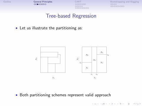
• Let us illustrate the partitioning as:

t1

t2

t3

t4

R1

R2

R3

R4

R5

X1X1X

2

X2

• Both partitioning schemes represent valid approach



• There is a number of possible ways to do the partitioning – letus restrict ourselves to recursive binary splitting scheme

• The binary split works as follows:

• First, we split the space into two halves• Then, we model the response by the mean in each region• The variable and threshold for split are chosen based on the

best response• Then, each region is further split (or not) using the same

procedure we did in the first step (i.e., recursion)• This process is applied up to a given stopping point



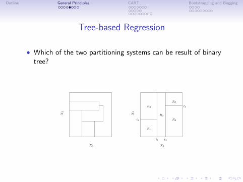
• Which of the two partitioning systems can be result of binarytree?

t1

t2

t3

t4

R1

R2

R3

R4

R5

X1X1

X2

X2



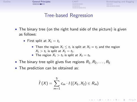
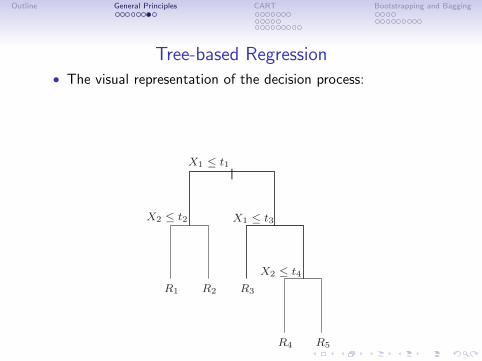
• The binary tree (on the right hand side of the picture) is givenas follows:

• First split at X1 = t1

• Then the region X1 ≤ t1 is split at X2 = t2 and the regionX1 > t1 is split at X1 = t3.

• The region X1 > t3 is split at X2 = t4.

• The binary tree split gives five regions R1,R2, . . . ,R5

• The prediction can be obtained as:

f (X ) =5∑

m=1

cm · I ((X1,X2) ∈ Rm)


Tree-based Regression• The visual representation of the decision process:

|

R1 R2 R3

R4 R5

X1 ≤ t1

X2 ≤ t2 X1 ≤ t3

X2 ≤ t4


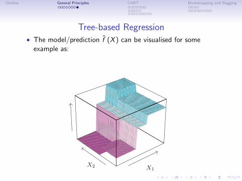
Tree-based Regression• The model/prediction f (X ) can be visualised for some

example as:

X1X2



• Thus, we have covered the idea for the regression tree in anut-shell

• In the following we focus in details on:

• How to grow Regression tree• How to grow Classification tree• Various topics


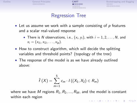
Regression Tree

• Let us assume we work with a sample consisting of p featuresand a scalar real-valued response

• There is N observations, i.e., (xi , yi ), with i = 1, 2, . . . ,N, andxi = (xi1, xi2, . . . , xip).

• How to construct algorithm, which will decide the splittingvariables and threshold points? (topology of the tree)

• The response of the model is as we have already outlinedabove:

f (X ) =5∑

m=1

cm · I ((X1,X2) ∈ Rm)

where we have M regions R1,R2, ...,RM , and the model is constantwithin each region


Regression Tree

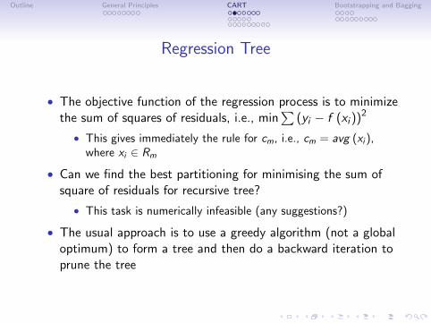
• The objective function of the regression process is to minimizethe sum of squares of residuals, i.e., min

∑(yi − f (xi ))2

• This gives immediately the rule for cm, i.e., cm = avg (xi ),where xi ∈ Rm

• Can we find the best partitioning for minimising the sum ofsquare of residuals for recursive tree?

• This task is numerically infeasible (any suggestions?)

• The usual approach is to use a greedy algorithm (not a globaloptimum) to form a tree and then do a backward iteration toprune the tree


Regression Tree

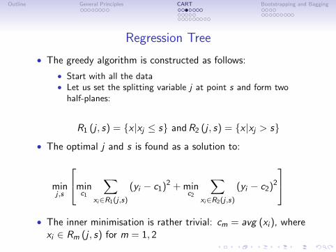
• The greedy algorithm is constructed as follows:

• Start with all the data• Let us set the splitting variable j at point s and form two

half-planes:

R1 (j , s) = {x |xj ≤ s} andR2 (j , s) = {x |xj > s}

• The optimal j and s is found as a solution to:

minj ,s

minc1

∑xi∈R1(j ,s)

(yi − c1)2 + minc2

∑xi∈R2(j ,s)

(yi − c2)2

• The inner minimisation is rather trivial: cm = avg (xi ), wherexi ∈ Rm (j , s) for m = 1, 2


Regression Tree

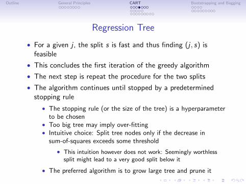
• For a given j , the split s is fast and thus finding (j , s) isfeasible

• This concludes the first iteration of the greedy algorithm

• The next step is repeat the procedure for the two splits

• The algorithm continues until stopped by a predeterminedstopping rule

• The stopping rule (or the size of the tree) is a hyperparameterto be chosen

• Too big tree may imply over-fitting• Intuitive choice: Split tree nodes only if the decrease in

sum-of-squares exceeds some threshold

• This intuition however does not work: Seemingly worthlesssplit might lead to a very good split below it

• The preferred algorithm is to grow large tree and prune it


Regression Tree

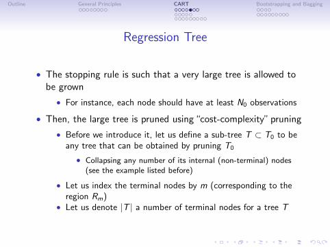
• The stopping rule is such that a very large tree is allowed tobe grown

• For instance, each node should have at least N0 observations

• Then, the large tree is pruned using “cost-complexity” pruning

• Before we introduce it, let us define a sub-tree T ⊂ T0 to beany tree that can be obtained by pruning T0

• Collapsing any number of its internal (non-terminal) nodes(see the example listed before)

• Let us index the terminal nodes by m (corresponding to theregion Rm)

• Let us denote |T | a number of terminal nodes for a tree T


Regression Tree

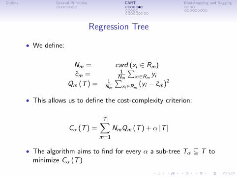
• We define:

Nm = card (xi ∈ Rm)cm = 1

Nm

∑xi∈Rm

yiQm (T ) = 1

Nm

∑xi∈Rm

(yi − cm)2

• This allows us to define the cost-complexity criterion:

Cα (T ) =

|T |∑m=1

NmQm (T ) + α |T |

• The algorithm aims to find for every α a sub-tree Tα j T tominimize Cα (T )


Regression Tree

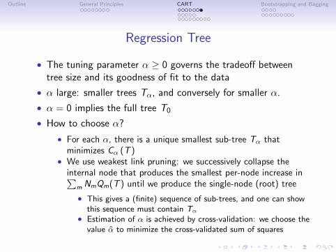
• The tuning parameter α ≥ 0 governs the tradeoff betweentree size and its goodness of fit to the data

• α large: smaller trees Tα, and conversely for smaller α.

• α = 0 implies the full tree T0

• How to choose α?

• For each α, there is a unique smallest sub-tree Tα thatminimizes Cα (T )

• We use weakest link pruning: we successively collapse theinternal node that produces the smallest per-node increase in∑

m NmQm(T ) until we produce the single-node (root) tree

• This gives a (finite) sequence of sub-trees, and one can showthis sequence must contain Tα

• Estimation of α is achieved by cross-validation: we choose thevalue α to minimize the cross-validated sum of squares


Classification Tree

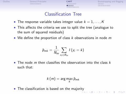
• The response variable takes integer value k = 1, . . . ,K

• This affects the criteria we use to split the tree (analogue tothe sum of squared residuals)

• We define the proportion of class k observations in node m

pmk =1

Nm

∑xi∈Rm

I (yi = k)

• The node m then classifies the observation into the class ksuch that:

k (m) = arg maxk

pmk

• The classification is based on the majority


Classification Tree

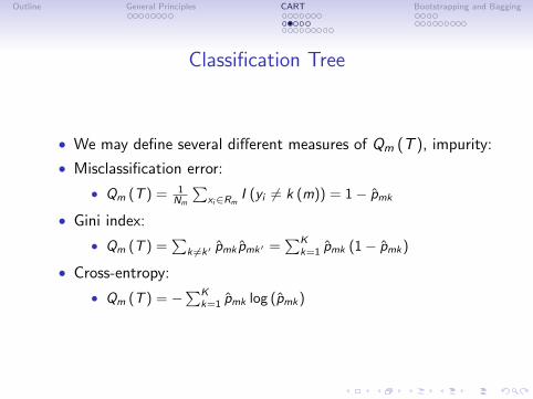
• We may define several different measures of Qm (T ), impurity:

• Misclassification error:

• Qm (T ) = 1Nm

∑xi∈Rm

I (yi 6= k (m)) = 1− pmk

• Gini index:

• Qm (T ) =∑

k 6=k′ pmk pmk′ =∑K

k=1 pmk (1− pmk)

• Cross-entropy:

• Qm (T ) = −∑K

k=1 pmk log (pmk)


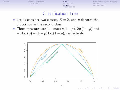
Classification Tree• Let us consider two classes, K = 2, and p denotes the

proportion in the second class• Three measures are 1−max (p, 1− p), 2p (1− p) and−p log (p)− (1− p) log (1− p), respectively

0.0 0.2 0.4 0.6 0.8 1.0

0.0

0.1

0.2

0.3

0.4

0.5

p

Entropy

Gini in

dex

Misclas

sifica

tion e

rror


Classification Tree

• Cross-entropy and the Gini index are more sensitive to changesin the node probabilities than the misclassification rate

• In a two-class problem with 400 observations in each class(denote this by (400, 400)), suppose one split created nodes(300, 100) and (100, 300), while the other created nodes (200,400) and (200, 0).

• Both splits produce a misclassification rate of 0.25, but thesecond split produces a pure node and is probably preferable

• Both the Gini index and cross-entropy are lower for the secondsplit

• The Gini index or cross-entropy should be used when growingthe tree

• To guide cost-complexity pruning, any of the three measurescan be used, but typically it is the misclassification rate


Classification Tree

• The Gini index can be interpreted in two interesting ways:

• Rather than classify observations to the majority class in thenode, we could classify them to class k with probability pmk

• The training error rate of this rule in the node is∑k 6=k′ pmk pmk′

• If we code each observation as 1 for class k and zerootherwise, the variance over the node of this 0− 1 response ispmk (1− pmk), summing over classes k again gives the Giniindex


Various Topics: Categorical Predictors

• Predictor having q possible unordered values – there are2q−1 − 1 possible partitions of the q values into two groups

• Computations become prohibitive for large q• For a 0− 1 outcome, the computation simplifies:

• Order the predictor classes according to the proportion fallingin outcome class 1

• Split this predictor as if it were an ordered predictor• This gives the optimal split, in terms of cross-entropy or Gini

index, among all possible 2q−1 − 1 splits• This result also holds for a quantitative outcome and square

error loss—the categories are ordered by increasing mean ofthe outcome

• For multicategory outcomes, no such simplifications arepossible, the partitioning algorithm tends to favor categoricalpredictors with many levels q


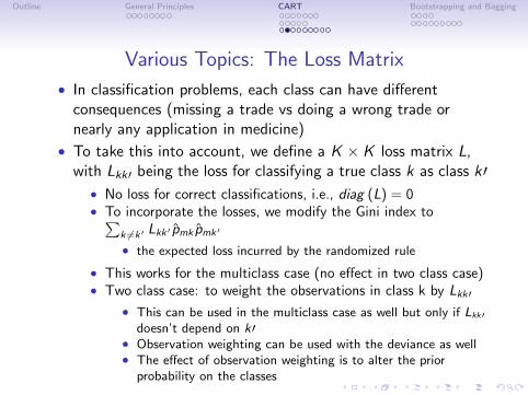
Various Topics: The Loss Matrix

• In classification problems, each class can have differentconsequences (missing a trade vs doing a wrong trade ornearly any application in medicine)

• To take this into account, we define a K × K loss matrix L,with Lkk′ being the loss for classifying a true class k as class k′• No loss for correct classifications, i.e., diag (L) = 0• To incorporate the losses, we modify the Gini index to∑

k 6=k′ Lkk′ pmk pmk′

• the expected loss incurred by the randomized rule

• This works for the multiclass case (no effect in two class case)• Two class case: to weight the observations in class k by Lkk′

• This can be used in the multiclass case as well but only if Lkk′doesn’t depend on k′

• Observation weighting can be used with the deviance as well• The effect of observation weighting is to alter the prior

probability on the classes


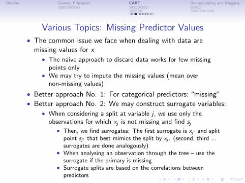
Various Topics: Missing Predictor Values• The common issue we face when dealing with data are

missing values for x

• The naive approach to discard data works for few missingpoints only

• We may try to impute the missing values (mean overnon-missing values)

• Better approach No. 1: For categorical predictors: “missing”• Better approach No. 2: We may construct surrogate variables:

• When considering a split at variable j , we use only theobservations for which xj is not missing and find sj• Then, we find surrogates: The first surrogate is xj′ and split

point sj′ that best mimics the split by xj . (second, third ...surrogates are done analogously)

• When analysing an observation through the tree – use thesurrogate if the primary is missing

• Surrogate splits are based on the correlations betweenpredictors


Various Topics: Beyond Binary Splits

• You can ask why binary splits?

• At each node into, we can use multiway splits into more than 2categories

• This can be useful but the biggest advantage lies in the factthat it fragments data too quickly

• In the subsequent levels, not enough data usually remains• This leaves any binary tree being preferable in general


Various Topics: Other Tree-Building Procedures

• The previous section introduced the CART (classification andregression tree) implementation of trees

• For further reference, the other popular methodology is ID3and its later versions, C4.5 and C5.0

• The most significant feature unique to C5.0: After a tree isgrown, the splitting rules that define the terminal nodes cansometimes be simplified

• One or more condition can be dropped without changing thesubset of observations

• This may result in simplified splitting rules• The resulting partitioning may not resemble a tree


Various Topics: Linear Combination Splits

• We may pose a question why to split along one variable andnot rather along linear combinations

• Instead of splitting xj ≤ s, we would split∑

ajxj≤s• The weights aj as well as the split point would be find during

optimization• This is possible solution but tree would be more difficult to

interpret

• A better way to use linear combination splits is in thehierarchical mixtures of experts (HME) model


Various Topics: Instability of Trees

• Major problem with trees is their high variance

• Small change in the data set can result in a very differentseries of splits

• This hurts the interpretability of the results

• The instability stems from the hierarchical nature of theprocess

• The error at the top of the tree close to the root propagatesthrough the whole tree

• Possible solution may be to search for more stable splitcriterion

• In general, this is a price for the simple tree-based structure

• Bagging averages many trees to reduce this variance

• The final part of the lecture addresses this issue in details


Various Topics: Lack of Smoothness

• We have seen in the previous slides that prediction is notsmooth (recall 2D surface)

• This comes from the nature of the model of finding R1,R2, . . .partitions

• The problem is not so strong for classification but is apparentfor regressions

• See MARS method, which can be viewed as a smoothmodification of the CART


Various Topics: Difficulty in Capturing Additive Structure

• Regression and Classification trees have difficulty in modelingadditive structure

• Let us illustrate it on a following regression case:

• The true model reads: Y = c1I (X1 < t1)) + c2I (X2 < t2) + ewhere e is a zero-mean noise

• The binary tree might make its first split on X2 around t2• The second split may be to split both nodes in X1 around t1• When dataset is small, this may not happen• The growing number of terms in the true model (c1, c2, . . . )

would require complex tree structure and large amount of data• The nature why the tree fails is the binary structure• See the MARS method for better solution in such a case


Bootstrapping and Tree Bagging

• General Idea: Instead of training one strong tree using thewhole data set, we train number of “weaker” trees on thesub-samples and average out the result

• The averaging out (independently constructed) trees reducesvariance and thus make the estimate more accurate

• The key element is that trees have to be independently grown

• Constructing a tree from a previous section and then obtainingthe set of sub-trees by different pruning does not help

• The tool to achieve this task is bootstrapping


Bootstrapping• Bootstrapping: In statistics, the bootstrap means random

sampling with replacement• The usual application is to estimate the properties of an

estimator (bias, variance, confidence intervals...)• Let us illustrate the bootstrap on the simple example: Let us

toss a coin and denote 1 when heads and 0 when tails. We areinterested in the properties of the estimator of average valuewhen we toss a coin N-times

• N-times tossing a coin means that we obtain a series ofx1, x2, . . . , xN , with xi = 0, 1

• The estimator is defined as µN = 1N

∑Ni=1 xi

• For two independent experiments (N tosses of a coin) weobtain different values

• What is its average value? What is a distribution of µN (whenwe repeat the experiment)?

• How to estimate the properties of the µN?


Bootstrapping• The route we follow is the bootstrapping procedure, where the

random sampling with replacement is done from the empiricaldistribution function• Create bootstrapped sample: N-random draws from

x1, x2, x3, . . . , xN• The resulting sample may look as follows:

Xa = x3, x4, x1, xN , x1, . . .• Calculate the estimator on the bootstrapped sample Xa,

denote it as µN,a

• Repeat the procedure for a = 1, 2, 3, . . . and collect the set ofµN,1, µN,2, µN,2, . . .

• The statistical properties µN can be deduced from thedistribution of µN,1, µN,2, µN,3, . . .

• The first moment, second moment,...• The percentiles of the distribution f (µN) can be derived in a

similar manner• Question: How would you construct the hypothesis about theµN being equal to ω?


Bootstrapping

• The properties of an estimator estimated without anyparametric assumptions

• The bootstrapping can be used for estimating properties inthe linear regression

• For an i-th observation, let us denote xi to be independentvariable (multidimensional), yi to be dependent variable

• Let us denote yi to be an estimated value for the dependentvariable using a model (regression) of interest and ei = yi − yithe residuals of the fit

• The bootstrapping is then performed on the residuals

• Fit the model for all i (i = 1, . . . , I ), collect ei• Sample with replacement a set of I values, denoted as

e1, e2, e3, . . .• Create bootstrapped dependent variables yi = yi + ei• Fit a new model of xi on yi and retain the variables of

interest from the fit• Estimate properties of the fit on the bootstrapped sample


Bootstrapping

• There is a number of extensions in the literature:

• Gaussian process regression bootstrap• Wild bootstrap• Block bootstrap• Bayesian bootstrap• White-noise bootstrap

• For time series (relevant in finance) with memory, theprocedure does not work

• See for example Maximum Non-Extensive Entropy BlockBootstrap for Non-Stationary Processes


Bagging

• Bootstrap was used to estimate the properties of theestimator (accuracy)

• We can use it to improve the prediction itself

• We use the example of a tree, but the procedure is general!• Bagging – bootstrap aggregation

• The bootstrap can be in the Bayesian framework linked to aposteriori average

• Let us outline the framework for the bootstrapping trees:

• Independent variable: xi• Dependent variable: yi• The training sample has N observations, .i.e,

Z = ((x1, y1) , (x2, y2) , . . . , (xN , yN))• The objective is a regression of y on x . The prediction

(estimate) of the dependent variable for an input x is denotedas f (x)


Bagging• Let us create a b-th bootstrap sample Z ∗b as a random sample

with replacement from Z , with b = 1, . . . ,B• Fit the model fb (x)• The bagging estimate of the model at x is defined as:

fbag (x) =1

B

∑b

fb (x) .

• Let us denote P the empirical distribution function, whichputs an equal probability on every observation (xi , yi )

• The true bagging estimate is EP f∗ (x) where

Z∗ = ((x∗1 , y∗1 ) , (x∗2 , y

∗2 ) , . . . , (x∗N , y

∗N)) and each pair coming

from P

• If the model f is an adaptive (non-linear) function of the data,fbag (x) will differ from f (x), otherwise fbag (x)→ f (x) asB →∞


Bagging and Trees

• Tree-based regression/classification is adaptive function to thedata

• For every bootstrapped sample, the regression tree is grown

• Since the data are different, the different tree is found

• Different number of terminal nodes• Different features involved in growing the tree• Different values for splitting (when the same features are used)

• The bagged tree estimate at input x is thus an average of Btrees grown on the B independent bootstrapped samples andestimated at point x


Bagging and Trees

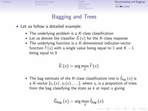
• Let us follow a detailed example:

• The underlying problem is a K -class classification• Let us denote the classifier G (x) for the K -class response• The underlying function is a K -dimensional indicator-vector

function f (x) with a single value being equal to 1 and K − 1being equal to 0

G (x) = arg maxk

f (x)

• The bag estimate of the K -class classification tree is fbag (x) isa K -vector [r1 (x) , r2 (x) , . . . ], where rk is a proportion of treesfrom the bag classifying the state as k at input x giving

Gbag (x) = arg maxk

fbag (x)


Bagging and Trees

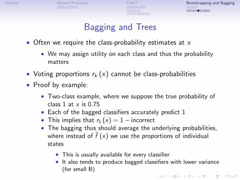
• Often we require the class-probability estimates at x

• We may assign utility on each class and thus the probabilitymatters

• Voting proportions rk (x) cannot be class-probabilities

• Proof by example:

• Two-class example, where we suppose the true probability ofclass 1 at x is 0.75

• Each of the bagged classifiers accurately predict 1• This implies that r1 (x) = 1 – incorrect• The bagging thus should average the underlying probabilities,

where instead of f (x) we use the proportions of individualstates

• This is usually available for every classifier• It also tends to produce bagged classifiers with lower variance

(for small B)


Bagging and Trees – Simulated Example

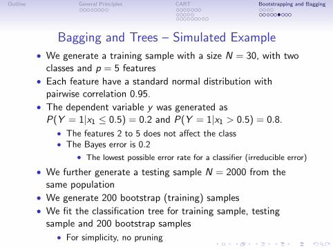
• We generate a training sample with a size N = 30, with twoclasses and p = 5 features

• Each feature have a standard normal distribution withpairwise correlation 0.95.

• The dependent variable y was generated asP(Y = 1|x1 ≤ 0.5) = 0.2 and P(Y = 1|x1 > 0.5) = 0.8.

• The features 2 to 5 does not affect the class• The Bayes error is 0.2

• The lowest possible error rate for a classifier (irreducible error)

• We further generate a testing sample N = 2000 from thesame population

• We generate 200 bootstrap (training) samples

• We fit the classification tree for training sample, testingsample and 200 bootstrap samples

• For simplicity, no pruning


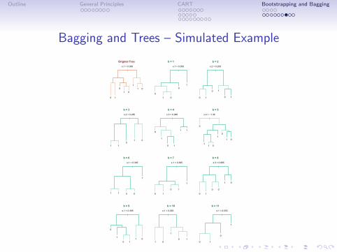
Bagging and Trees – Simulated Example

|

x.1 < 0.395

0 1

01 0

11 0

Original Tree

|

x.1 < 0.555

0

1 0

01

b = 1

|

x.2 < 0.205

0 1

0 1

0 1

b = 2

|

x.2 < 0.285

1 10

1 0

b = 3

|

x.3 < 0.985

0

1

0 1

1 1

b = 4

|

x.4 < −1.36

0

11 0

10

1 0

b = 5

|

x.1 < 0.395

1 1 0 0

1

b = 6

|

x.1 < 0.395

0 1

0 1

1

b = 7

|

x.3 < 0.985

0 1

0 0

1 0

b = 8

|

x.1 < 0.395

0

1

0 11 0

b = 9

|

x.1 < 0.555

1 0

1

0 1

b = 10

|

x.1 < 0.555

0 1

0

1

b = 11


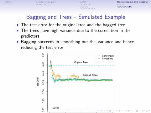
Bagging and Trees – Simulated Example• The test error for the original tree and the bagged tree• The trees have high variance due to the correlation in the

predictors• Bagging succeeds in smoothing out this variance and hence

reducing the test error

0 50 100 150 200

0.20

0.25

0.30

0.35

0.40

0.45

0.50

Number of Bootstrap Samples

Test

Err

or

Bagged Trees

Original Tree

Bayes

ConsensusProbability


References

Trevor Hastie, Robert Tibshirani, Jerome H. Friedman, TheElements of Statistical Learning, 2001 (available online)

Documents

Decision Trees and Forests Data Analysis and Machine … General Principles CART Bootstrapping and Bagging Decision Trees and Forests Data Analysis and Machine Learning ... To guide