Embed Size (px)
Citation preview
DECLARATION AND CERTIFICATION
Except where mentioned, we verify that the experimental work, results, analysis
and conclusions are set out in this project is entirely our own efforts.
MFO 04/2012 –large deflections of beams. Laboratory validation of proposed
project.
ACHOLA KEVIN : F18/1887/2007
…………………………………………………
ONUNGA ERICK: F18/1857/2007
………………………………………………..
KIRUGUMI DANIEL: F18/20991/2007
…………………………………………………
The above named students have submitted this report to the department of
Mechanical and manufacturing Engineering, University of Nairobi with my
approval as the supervisor (s)
Professor Oduori F.M Engineer Munyasi D.M
………………………… …………………………….

ii | P a g e
DEDICATION
We dedicate this project to human prosperity and enlightenment.
iii | P a g e
Abstract
The deflection of a large cantilever beam made of linear elastic aluminum under the
action of a vertical concentrated load applied at mid span was analyzed .this was
done experimentally and numerically using Professor Oduori’s1 theory of large
beam deflections.
The experiment was done using aluminum beam of dimension length 47cm by 5cm
and thickness of 1.7cm
From first principles, we derived the equation for the determination of large
deflection of beams. We set up tests in the laboratory in order to validate the theory;
we then compared theoretical and experimental results. They were in good
agreement.
1Professor department of mechanical and manufacturing engineering university of Nairobi

iv | P a g e
Acknowledgements
We take this opportunity to express our thanks to Professor Oduori and Engineer
Munyasi for their inspiration, support and the appreciation for their work under
taken in this project .we also express sincere gratitude to the staff at the
mechanical engineering workshop. We also appreciate the moral and general
support accorded to us by our friends.

v | P a g e
Nomenclature
b -Breath of the specimen
d –Thickness of the specimen (depth)
E –Young’s modulus
F –Force causing deflection of the beam
I –Second moment of area elasticity of aluminum
L, M –Coordinates perpendicular to, and parallel to the force causing deflection of
aluminum
M –Bending moment
P – Axial force
q – Uniformly distributed load
R –Radius of curvature
S – Length along the deflected cantilever beam
w, y -deflection
X, Y –Cartesian coordinates in the plane respectively
ɸ - Angular deformation of the deflected cantilever beam
σb – Bending stress
vi | P a g e
Table of contents
Declaration and certification ………………………………………………………….......i
Dedication ……………………………………………………………………………………ii
Abstract ………………………………………………………………………………………iii
Acknowledgements ………………………………………………………………………....iv
Nomenclature ………………………………………………………………………………..v
Chapter One 1.0 Introduction …………………………………………………………………………….1
1.1Assumptions………………………..…………………………………………………...3
1.2Objective ………………………………………………………………………………..4
Chapter Two 2.0 Literature review………………………………………………………………………5
2.1Theoretical Analysis ………………………………………………………………6
2.2 Formulation of the model ………………………………………………………..21
2.3 Model Validation and adaptation for laboratory experimentation ……….28
Chapter Three 3.0 Description of apparatus used ………………………………………………………32
3.1 Hand tools …………………………………..……………………………………...32
3.1.1 Tape measure ……………………………………………………………………32
3.1.2 Steel rule …………………………………………………………………………32
3.1.3 Vernier calipers …………………………………………………………………32
3.1.4 Vernier Height gauge ……………………………………………….………….32
3.1.5 Try-square ………………………………………………………………………..33
3.1.6 Dial gauge ………………………………………………………………………..33
3.1.7 Rough and smooth file …………………………………………………………33
3.1.8 Spirit level ………………………………………………………………………..34
vii | P a g e
3.1.9 Scriber …………………………………………………………………………….34
3.2 Machines ……………………………………………………………………………….35
3.2.1 Power hacksaw ………………………………………………....................35
3.2.2 Lathe machines ……………………………………………………………36
3.2.3 Milling machine ……………………………………………………………37
3.2.4 Planar machine …………………………………………………………….38
3.2.5 TIC machine ………………………………………………………………..38
Chapter four
4.0 laboratory data acquisition …………………………………………………………..40
4.1 specimen preparation …………………………………………………………….40
4.1.1 Procedure of preparation ……………………………………………………40
4.2 Test Rig preparation ………………………………………………………………42
4.2.1 Preparation of the support roller bearings..………………………………43
4.3 Test of specimen ……………………………………………………………………45
Chapter five
5.0 Analysis of experimental results……………………………………………………..51
5.1 Results ………………………………………………...…………………………….52
5.2 Data analysis ……………………………………………………………………….56
5.2.1 Sample calculation…………………………………………………………….56
Chapter Six 6.0 Discussion, conclusion and recommendations …………………………….………………66
6.1 Discussions …………………………………………………………………………………66
6.2 Conclusion …………………………………………….....................................................67
6.3 Recommendations for further work …………………………………………………….68
7.0 References …………………………………………………….…………………………….69

viii | P a g e
Table of figures
Figure page
Fig 1 crop stem deflected by the reel……………………………………………………………………………………………………2
Fig 2 diagrammatic representation of deflected beam ……………………………………………………………………….6
Fig 3 bending of Euler-Bernoulli beam …………………………………………………………………………………………………8
Fig 4 elastic curve derivation ……………………………………………………………………………………………………………….11
Fig 5 triangle CDQ ……………………………………………………………………………………………………………………………….11
Fig 6 first area principle (semi-graphic form) .........................................................................................15
Fig 7 large deflections of buckled bars (the elastica) …….……………………………………………………………………..16
Fig 8 model of deflection ……………………………………………..……………………………………………………………………..21
Fig 9 transformed model of deflected stem ……………..………………………………………………………………………..23
Fig 10 triangle ABC ……………………………………………………………………………………………………………………………..26
Fig 11 the model adopted for laboratory validation …………………………………………………………………………..28
Fig 12 transformed model adopted for laboratory validation …………………………………………………………….29
Fig 13 force diagram ………………………………………………………………………………………………………………………….30
Fig 14 loading arrangement ………………………………………………………………………………………………………………50
Fig 15 deflections in progress ……………………………………………………………………………………………………………50
Fig 16 triangle adapted for data analysis …………………………………………………………………………………………..56
Fig 17 beam cross section …………………………………………………………………………………………………………………57
ix | P a g e
Table of pictures
Unless otherwise stated all pictures were taken at the department of mechanical and manufacturing
Engineering workshop at the university of Nairobi.
Picture page
Picture 1 vernier height gauge ……………………………………………………………………………………………………….33
Picture 2 power hacksaw ……………………………………………………………………………………………………………….35
Picture 3 and 4 lathe machines ………………………………………………………………………………………………………36
Picture 4 milling machine ……………………………………………………………………………………………………………….37
Picture 5 planar machine ……………………………………………………………………………………………………………….38
Picture 6 TIC machine …………………………………………………………………………………………………………………….39
Picture 7 the unprepared aluminium beam ……………………………………………………………………………………40
Picture 8 aluminium bar on the planar workstation ……………………………………………………………………….41
Picture 9 aluminium beam after preparation …………………………………………………………………………………42
Picture 10 cast iron block with roller bearing supports ………………………………………………………………….43
Picture 11 roller bearings ………………………………………………………………………………………………………………44
Picture 12 knife-edge …………………………………………………………………………………………………………………….45
Picture 13 loading tip (knife-edge) 2 ……………………………………………………………………………………………..46
Picture 14 roller bearings on each groove …………………………………………………………………………………….47
Picture 15 loading arrangement ……………………………………………………………………………………………………48
Picture 16 the general arrangement on a TIC machine ………………………………………………………………..49
x | P a g e
Table of tables
Table page
Table 1: experimental raw data …………………………………………………………………………………………………52
Table 2: load and respective deflection (Experimental) …………………………………………………………….53
Table 3: table of analyzed values …...............................................................................................58
Table 4: load and calculated deflection ……………………………………………………………………………………..61
Table 5: comparisons between experimental and calculated values of deflections …………………..62
Table 6: load and percentage deviations ……………………………………………………………………………………65
xi | P a g e
Table of graphs
Graph page
Graph 1: of load against deflection ……………………………………………………………………………………………………54
Graph 2: for load against deflection for the elastic region………………………………………………………………..55
Graph 3: of
………………………………………………………………………………………..59
Graph 4: of calculated deflection against experimental deflection …..................................................63

1 | P a g e
Chapter one
1.0 Introduction Beams are common elements of many architectural, civil and mechanical engineering
structures and the study of the bending of straight beams forms an important and
essential part of the study of the broad field of mechanics of materials and structural
mechanics. All undergraduate courses on these topics include the analysis of the
bending of beam but only small deflections of the beam are usually considered. In such
a case, the differential equation that governs the behavior of the beam is linear and can
easily be solved. Here we consider large deflections in cantilever beams.
By definition beams are structural members capable of sustaining loads normal to their
axis, a cantilever beam is a beam that is fixed at one end, while the other end is
unsupported but suspended.
A beam in application may be strong enough to resist safely the bending moments due
to applied load yet not be suitable because its deflection is too great. Excessive
deflection may impair the strength and stability of the structure giving rise to minor
troubles such as cracking as well as affecting the functional needs and aesthetic
requirements. Thus, there is always a need to consider deflection when designing
beams.
In much of the study and practice of mechanical and structural engineering, the
equations used for determination of beam deflections, are derived with assumption of
small deflections .This is appropriate because, in most mechanical and structural
engineering applications, small deflections are a functional requirement. However, there
arise cases in agricultural machinery engineering for instance, where beam deflections
can no longer be assumed small. Then, it becomes necessary to develop and use
equations other than those commonly found in mechanical and structural1 engineering
documents, which are largely based on small deflections. Timoshenko and Gere
derived solutions to large deflection problems, which led to an elliptical integral. Elliptical
integral problems can only be evaluated numerically, which is tedious and long. Hence,
there is sufficient reason therefore to seek analytical solutions to problems of large
deflections .such an equation is developed and evaluated in this presentation.
An example of an application that would involve large crop stem (beam) deflections, in
the design and operation of the combine harvester reel as illustrated in fig 1.10
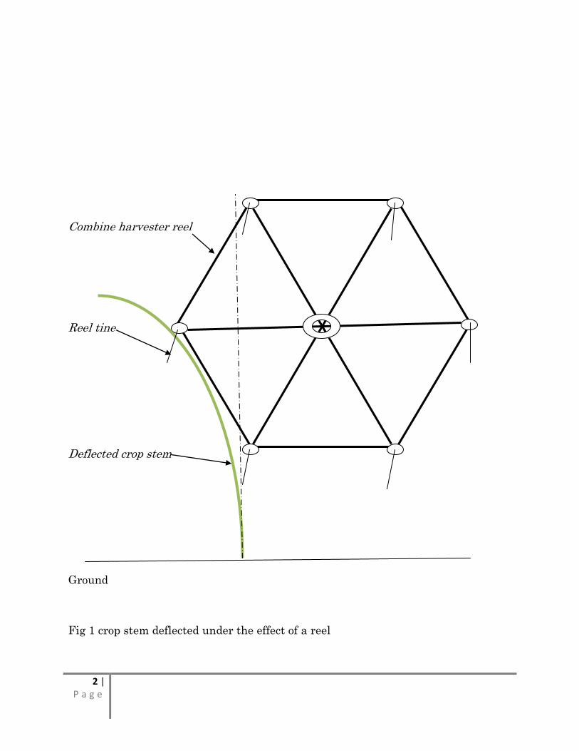
2 | P a g e
Combine harvester reel
Reel tine
Deflected crop stem
Ground
Fig 1 crop stem deflected under the effect of a reel
3 | P a g e
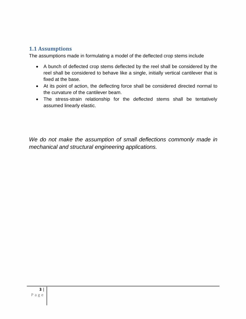
1.1 Assumptions
The assumptions made in formulating a model of the deflected crop stems include
A bunch of deflected crop stems deflected by the reel shall be considered by the
reel shall be considered to behave like a single, initially vertical cantilever that is
fixed at the base.
At its point of action, the deflecting force shall be considered directed normal to
the curvature of the cantilever beam.
The stress-strain relationship for the deflected stems shall be tentatively
assumed linearly elastic.
We do not make the assumption of small deflections commonly made in
mechanical and structural engineering applications.

4 | P a g e
1.2 Objective The purpose of this work is to validate a new theory for the determination of large beam
deflections of a class of cantilever beams under the action of a concentrated force or
load. This is done both experimentally and theoretically then the results compared to
ascertain the validity of the theory and hence formula presented for use in deriving
solutions analytically to large beam deflections.
5 | P a g e
Chapter two
2.0 Literature review In the literature, large deflections behavior of beams continues to be the subject of
intensive research. Numerous researchers have studied the problem under different
conditions and using different conditions and methods of solutions
Jong-Dar Yau developed closed-form solutions of large deflections for a guyed
cantilever column pulled by an inclined cable. He used elliptical integral method in
deriving analytical solution for tip displacement of the guyed column. His theory
can be useful in cable-stayed bridges, radio masts and cable supported roofs all of
which involve large deflections.
N. Tolou and J.L. Herder developed a semi analytical approach to large deflections
in compliant beams under point load. In their work, they successfully investigated
the feasibility of ADM (Adomian decomposition method) in analyzing compliant
mechanisms.
A.Kimiaeifar, G. Domairry, S.R. Mohebpour, A.R. Sohouli and A.G Davodi4
developed analytical solutions for large deflection of a cantilever beam under a non-
conservative load based on homotopy analysis method (HAM)
Stephen P. Timoshenko and James M. Gere1 analyzed large deflections by
considering the case of buckled bars (the elastica)
6 | P a g e
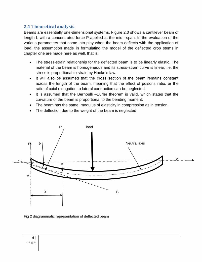
2.1 Theoretical analysis Beams are essentially one-dimensional systems. Figure 2.0 shows a cantilever beam of
length L with a concentrated force P applied at the mid –span. In the evaluation of the
various parameters that come into play when the beam deflects with the application of
load, the assumption made in formulating the model of the deflected crop stems in
chapter one are made here as well, that is:
The stress-strain relationship for the deflected beam is to be linearly elastic. The
material of the beam is homogeneous and its stress-strain curve is linear, i.e. the
stress is proportional to strain by Hooke’s law.
It will also be assumed that the cross section of the beam remains constant
across the length of the beam, meaning that the effect of poisons ratio, or the
ratio of axial elongation to lateral contraction can be neglected.
It is assumed that the Bernoulli –Eurler theorem is valid, which states that the
curvature of the beam is proportional to the bending moment.
The beam has the same modulus of elasticity in compression as in tension
The deflection due to the weight of the beam is neglected
R load
y ɸ Neutral axis
X
A
X B
Fig 2 diagrammatic representation of deflected beam
7 | P a g e
Several beam theories are in use to calculate and analyze deflections of beams under
the action of different kinds of loading .The most common ones are Eurler-Bernoulli
beam theory and Timoshenko beam theory.
Euler-Bernoulli beam theory which is also known as engineers beam theory or
classical beam theory is a simplification of the linear theory of elasticity which provides a
means of calculating the load –carrying and deflection characteristics of beams .It
covers the case for small deflections of the beam which is subjected to lateral loads
only.
Timoshenko beam theory covers beams under both lateral and axial loading.
8 | P a g e
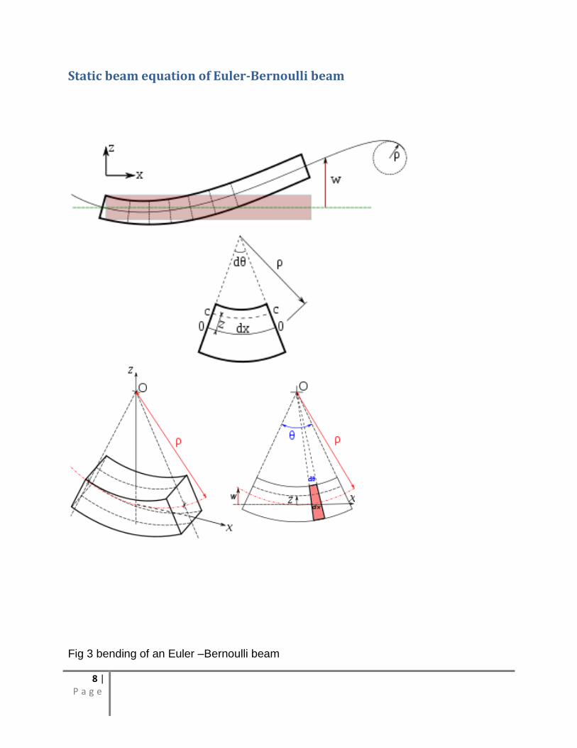
Static beam equation of Euler-Bernoulli beam
Fig 3 bending of an Euler –Bernoulli beam
9 | P a g e
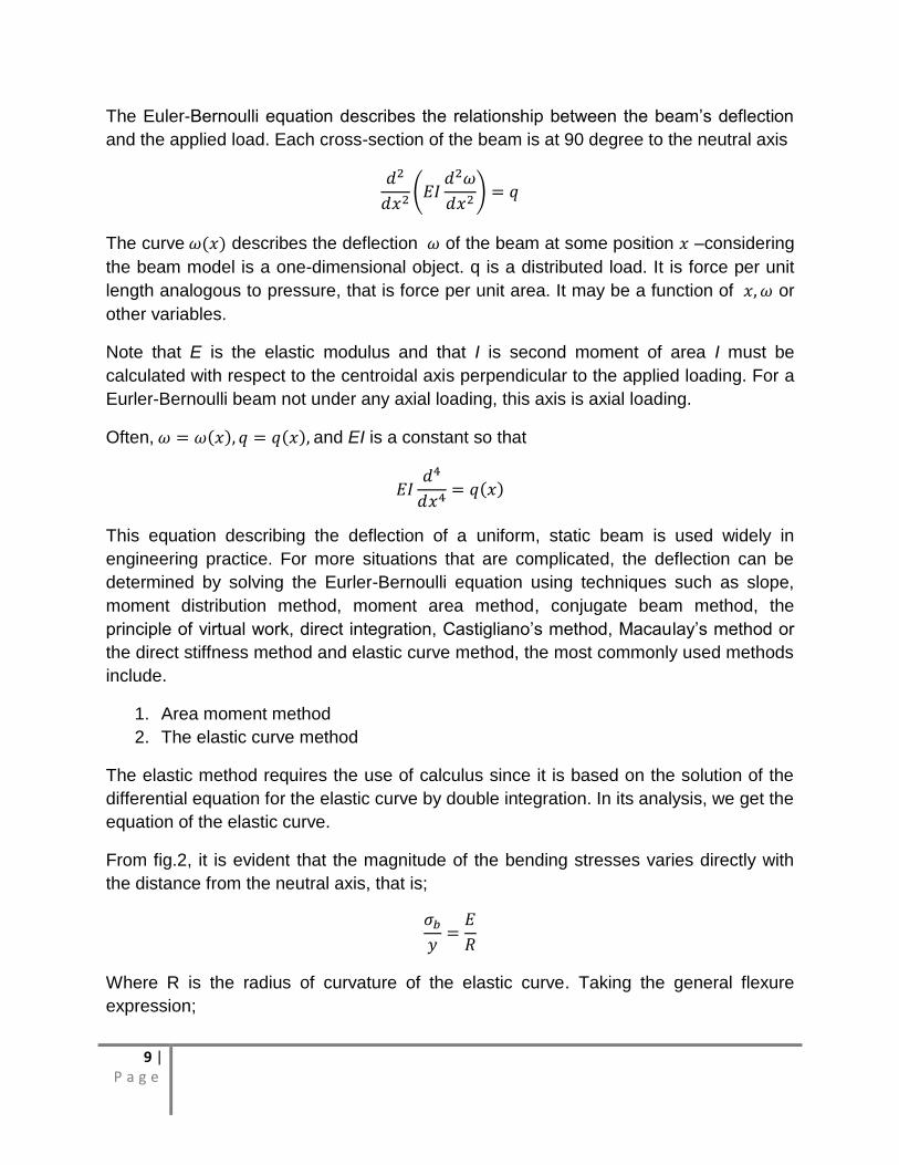
The Euler-Bernoulli equation describes the relationship between the beam’s deflection
and the applied load. Each cross-section of the beam is at 90 degree to the neutral axis
The curve describes the deflection of the beam at some position –considering
the beam model is a one-dimensional object. q is a distributed load. It is force per unit
length analogous to pressure, that is force per unit area. It may be a function of or
other variables.
Note that E is the elastic modulus and that I is second moment of area I must be
calculated with respect to the centroidal axis perpendicular to the applied loading. For a
Eurler-Bernoulli beam not under any axial loading, this axis is axial loading.
Often, and EI is a constant so that
This equation describing the deflection of a uniform, static beam is used widely in
engineering practice. For more situations that are complicated, the deflection can be
determined by solving the Eurler-Bernoulli equation using techniques such as slope,
moment distribution method, moment area method, conjugate beam method, the
principle of virtual work, direct integration, Castigliano’s method, Macaulay’s method or
the direct stiffness method and elastic curve method, the most commonly used methods
include.
1. Area moment method
2. The elastic curve method
The elastic method requires the use of calculus since it is based on the solution of the
differential equation for the elastic curve by double integration. In its analysis, we get the
equation of the elastic curve.
From fig.2, it is evident that the magnitude of the bending stresses varies directly with
the distance from the neutral axis, that is;
Where R is the radius of curvature of the elastic curve. Taking the general flexure
expression;

10 | P a g e
Then
Now consider unloaded beam AB as shown in fig 4, the beam is deflects to A1B1 under
a load q.
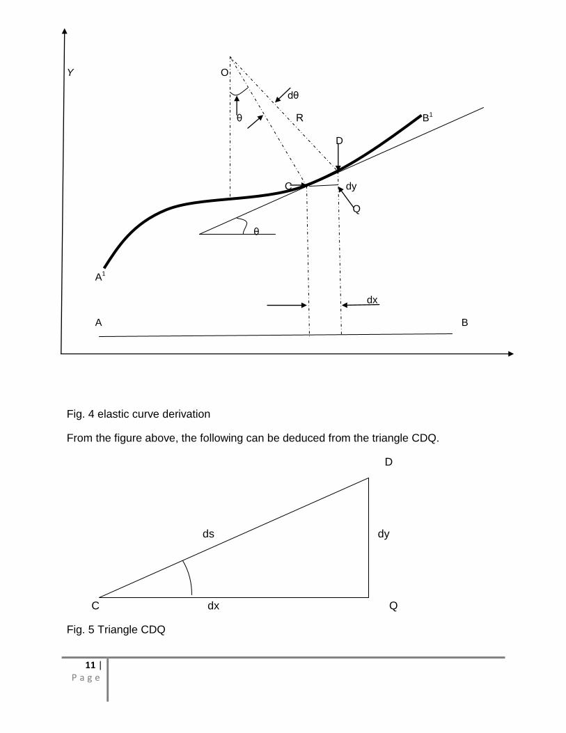
11 | P a g e
Y O
dθ
θ R B1
D
C dy
Q
θ
A1
dx
A B
Fig. 4 elastic curve derivation
From the figure above, the following can be deduced from the triangle CDQ.
D
ds dy
C dx Q
Fig. 5 Triangle CDQ
12 | P a g e
CD=
For small angle of θ
The curved line A1B1 in fig.3 represents the neutral surface of a beam after bending .It is
the elastic surface of a deflected beam of indefinite length. C and D are points on this
elastic surface and are separated by a small distance
When two lines are constructed perpendicular to the elastic curve at points C and D,
their extensions will intersect at the centre of curvature O, a distance R from the
curvature and will form a small angle,
The curvature is actually very slight; therefore, CQ can replace the horizontal length
Then from geometry
However, since triangle CDQ is small
And
Therefore,
13 | P a g e
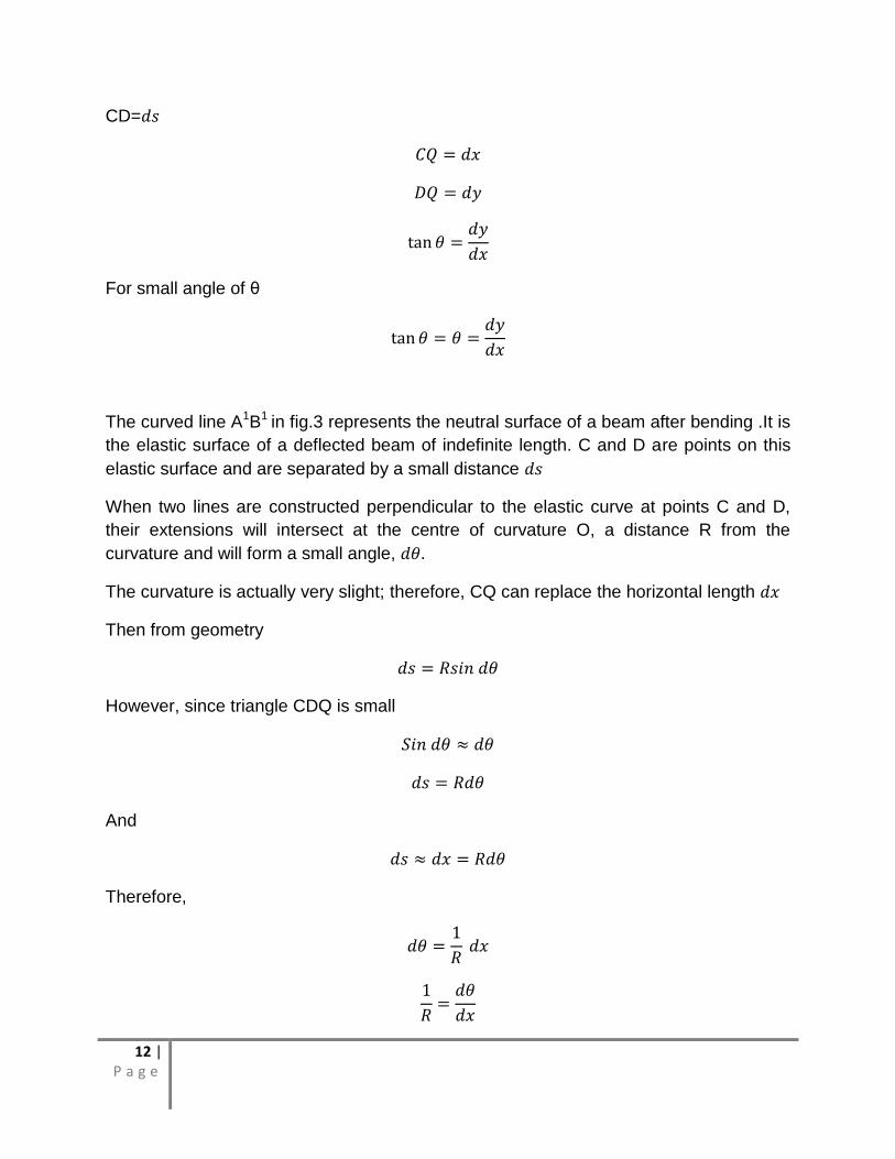
But
Substituting and evaluating, we get the differential equation of elastic curve as shown
below
From the general flexural equation
Hence,
Where
EI-is the flexural stiffness
- is the curvature of the neutral axis
In the above derivation of the elementary theory, the assumption of small deflections
has been made. Hence, this equation cannot be used in analyzing large beam
deflections problems. The elementary theory also neglects the square of the first
derivative in the curvature formula and provides no correction for the shortening of the
moment arm as the loaded end of the beam deflects.
From the area moment principle, the neutral surface of a homogeneous beam is
considered to be on a continuous plane, which passes through the centre of gravity of

14 | P a g e
each right section. When the beam deflects, the neutral surface becomes a continuous
curved surface. Deflections are measured from the original position of the neutral
surface to the elastic surface.
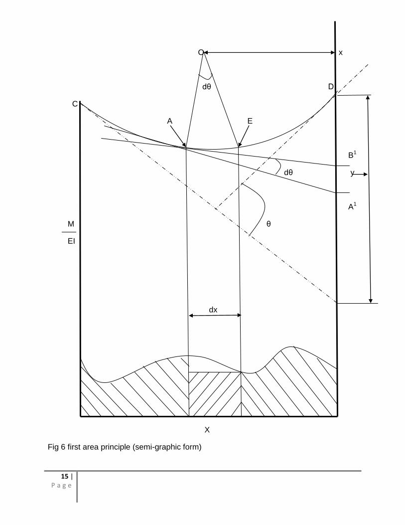
The derivation of the area moment equations is shown in the semi-graphic form in fig 6
15 | P a g e
O x
dθ D
C
A E
B1
dθ y
A1
M θ
EI
dx
X
Fig 6 first area principle (semi-graphic form)
16 | P a g e
From fig.6, the angle between the two tangents AA1 and BB1 is equal to . And the
summation of all elemental areas of the
diagram between the two tangent points (the
cross hatched area shown) is presented in equation form as .
This is the first area moment. it considers the assumptions of small deflections and thus
cannot be used to determine large deflections .
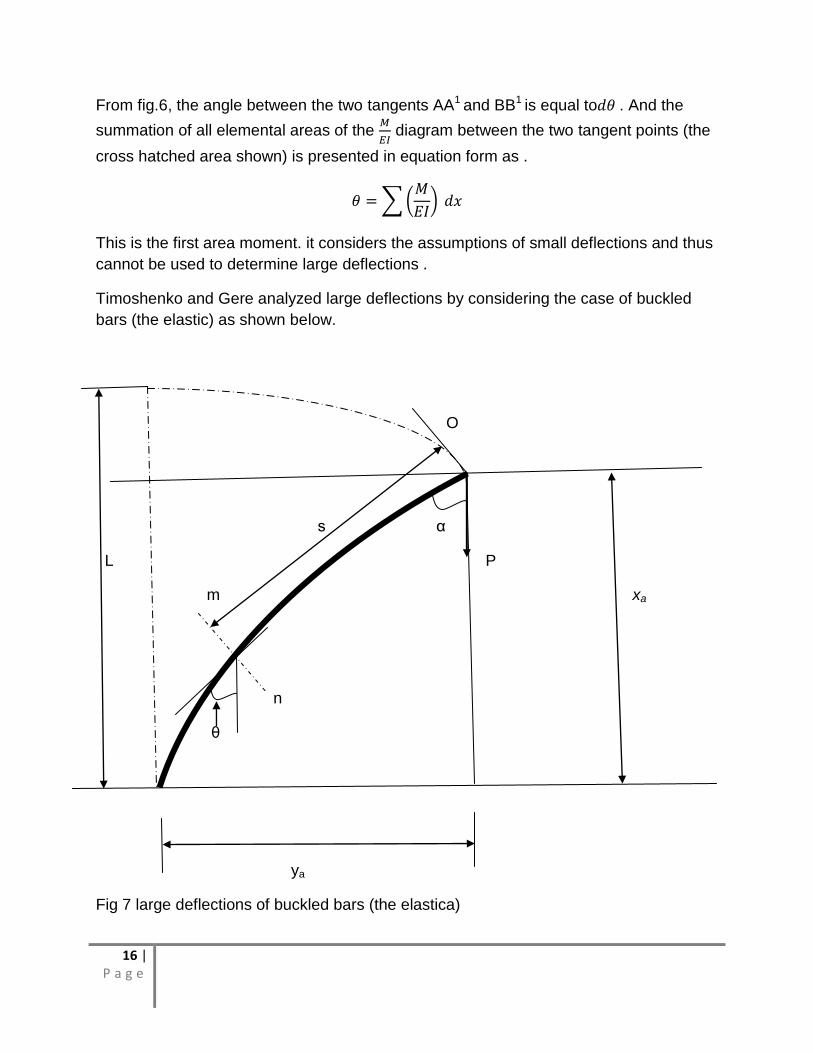
Timoshenko and Gere analyzed large deflections by considering the case of buckled
bars (the elastic) as shown below.
O
s α
L P
m xa
n
θ
ya
Fig 7 large deflections of buckled bars (the elastica)
17 | P a g e
At the critical loading, the bar can have any value of deflection, provided the deflection
remains small, the differential equations used to calculate the critical loads are based on
the approximate expression
for the curvature of the buckled bar. If the exact
expression for the curvature is used, there will be no indefiniteness in the value of
deflection. The shape of the elastic curve, when found from the exact differential
equation is called the elastica.
Consider the slender rod shown in fig.7, which is fixed at the base and free at the upper
end. If the load P is taken somewhat larger than the critical value, a large deflection of
the bar is produced. Taking the axis as shown in the figure and measuring the distance
s along the axis of the bar from the origin O, we find that the exact expression for the
radius of the curvature of the bar is
Since the bending moment in the bar is equal to the product of flexural rigidity the
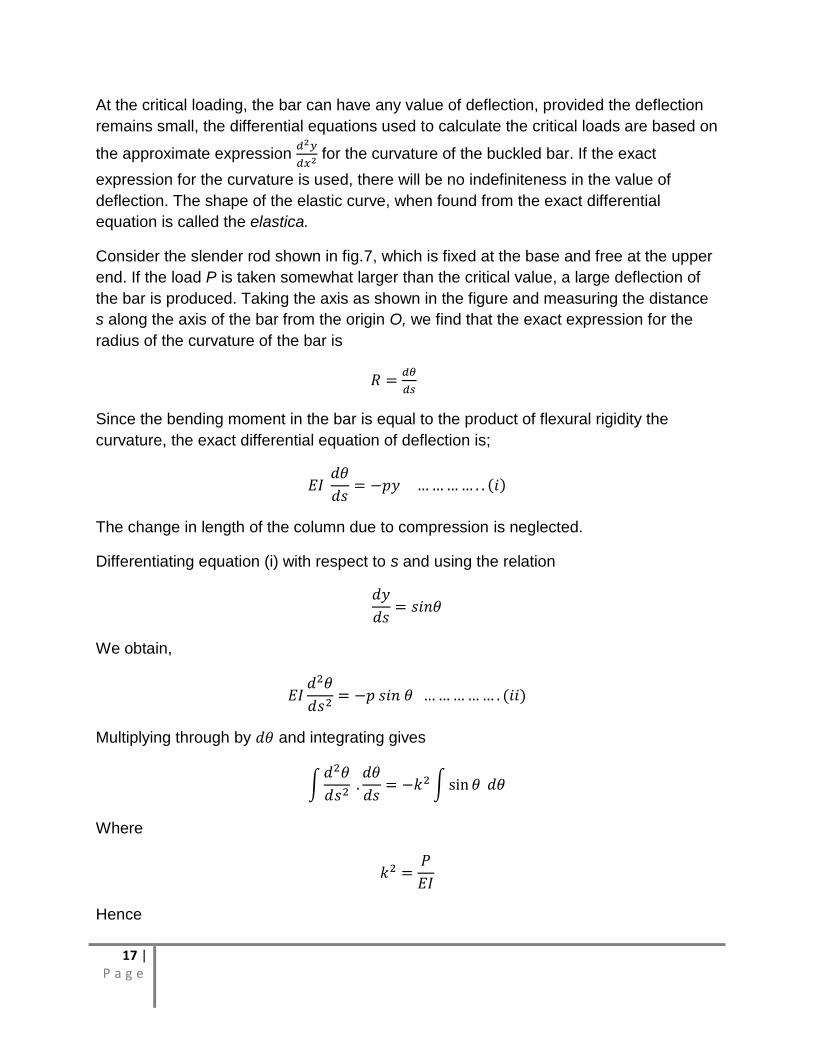
curvature, the exact differential equation of deflection is;
The change in length of the column due to compression is neglected.
Differentiating equation (i) with respect to s and using the relation
We obtain,
Multiplying through by and integrating gives
Where
Hence
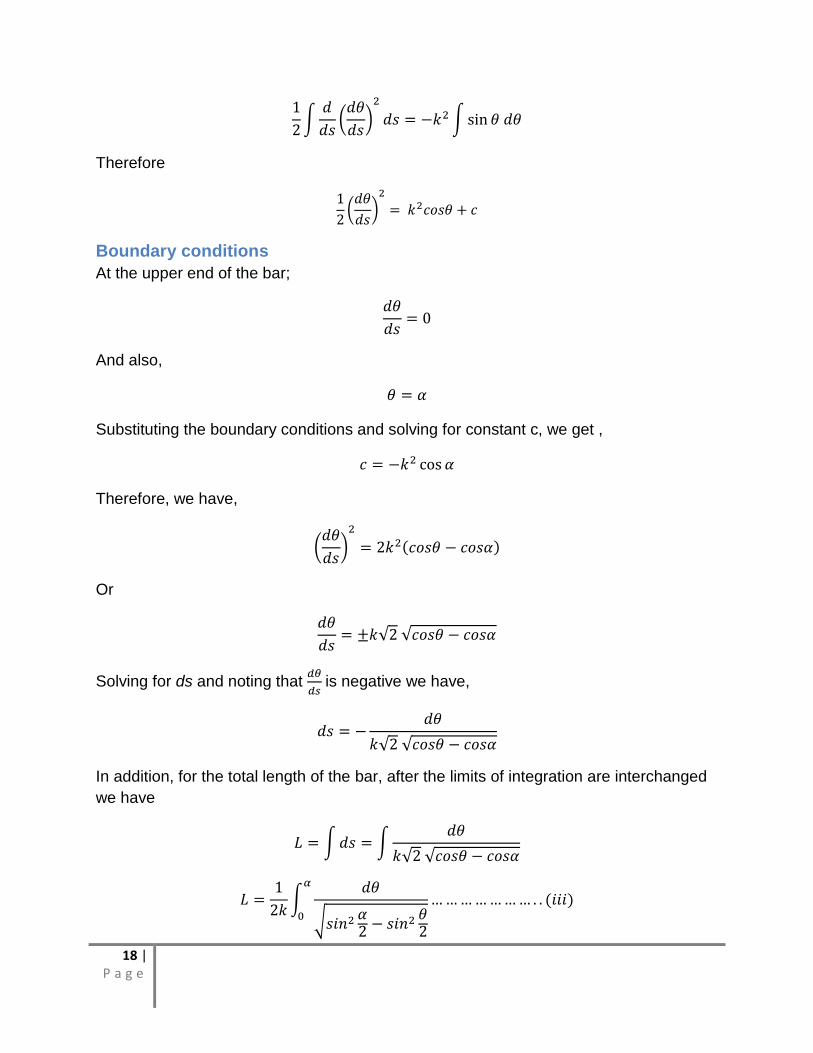
18 | P a g e
Therefore
Boundary conditions
At the upper end of the bar;
And also,
Substituting the boundary conditions and solving for constant c, we get ,
Therefore, we have,
Or
Solving for ds and noting that
is negative we have,
In addition, for the total length of the bar, after the limits of integration are interchanged
we have
19 | P a g e
Introducing ɸ and letting
such that,
Differentiating equation
Substituting equation (iii) and noting that
We obtain
As the value of decrease, the integral K and the load P increase
In calculating the deflection of the bar, we note that
The total deflection of the top of the top of the bar in the horizontal direction becomes
From equation (iv) we have;
And therefore,
ɸ
By using the relation,

20 | P a g e
We find that;
Substituting expression (v)(vi) and (ix) into equation (viii) and changing the limits
accordingly, we obtain;
21 | P a g e
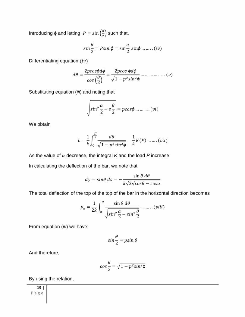
2.2 Formulation of the model However, the integral appearing in equation (vii) is known as a complete elliptical
integral of the first kind and is designated by K (p). Elliptical integrals can only be
evaluated numerically which is both tedious and does not give very accurate results. In
contrast, the introduction of L as the variable of integration instead of s greatly simplifies
the problem.
Hence, analytical solutions are sought to problems of large deflections. In this case, a
cantilever beam is considered fixed horizontally and a point load applied near the free
end such that the beam deflects upwards.
Ym
Fcos ɸm
dy Y
Beam dx
ds
r + dr
dɸ r X Xm
ɸ
Fig 8 model of deflection
22 | P a g e
The assumptions of small deflections commonly made in mechanical and structural
engineering are not made here.
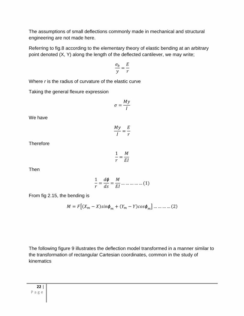
Referring to fig.8 according to the elementary theory of elastic bending at an arbitrary
point denoted (X, Y) along the length of the deflected cantilever, we may write;
Where r is the radius of curvature of the elastic curve
Taking the general flexure expression
We have
Therefore
Then
From fig 2.15, the bending is
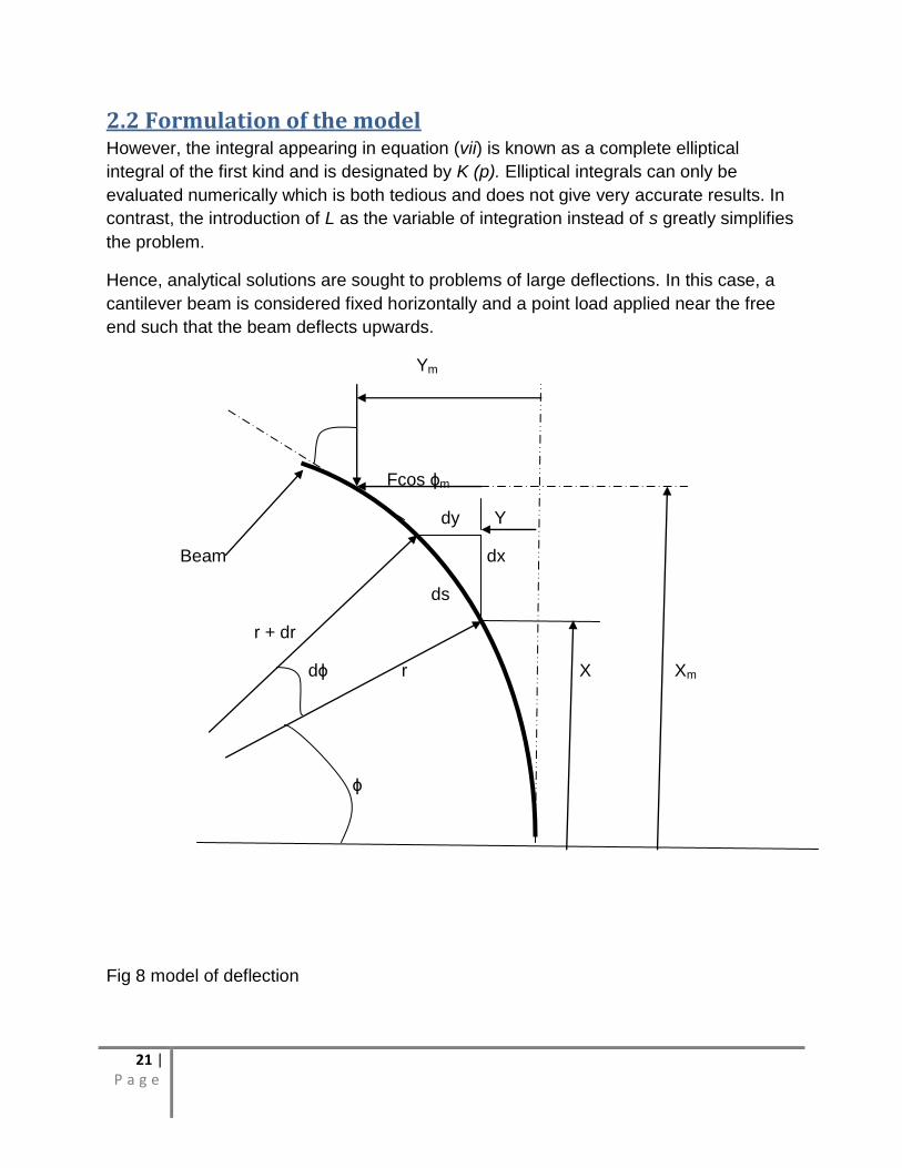
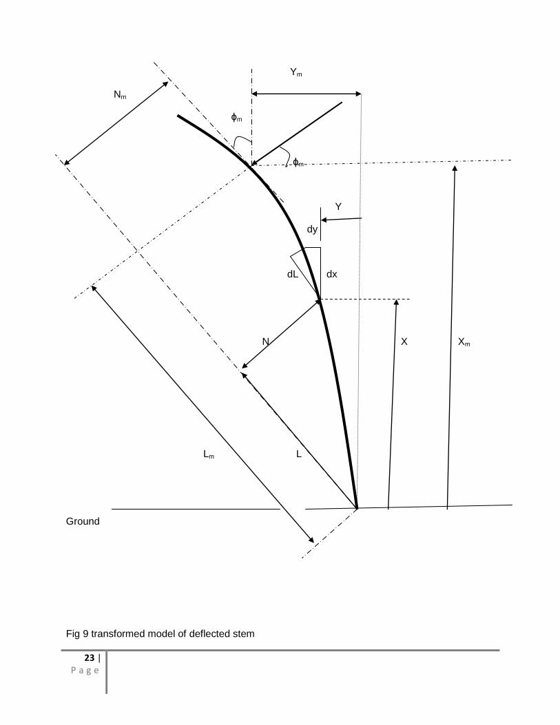
The following figure 9 illustrates the deflection model transformed in a manner similar to
the transformation of rectangular Cartesian coordinates, common in the study of
kinematics
23 | P a g e
Ym
Nm
ɸm
ɸm
Y
dy
dL dx
N X Xm
Lm L
Ground
Fig 9 transformed model of deflected stem
24 | P a g e
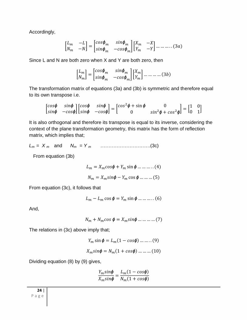
Accordingly,
Since L and N are both zero when X and Y are both zero, then
The transformation matrix of equations (3a) and (3b) is symmetric and therefore equal
to its own transpose i.e.
It is also orthogonal and therefore its transpose is equal to its inverse, considering the
context of the plane transformation geometry, this matrix has the form of reflection
matrix, which implies that;
Lm = X m and Nm = Y m ………………………….(3c)
From equation (3b)
From equation (3c), it follows that
And,
The relations in (3c) above imply that;
Dividing equation (8) by (9) gives,
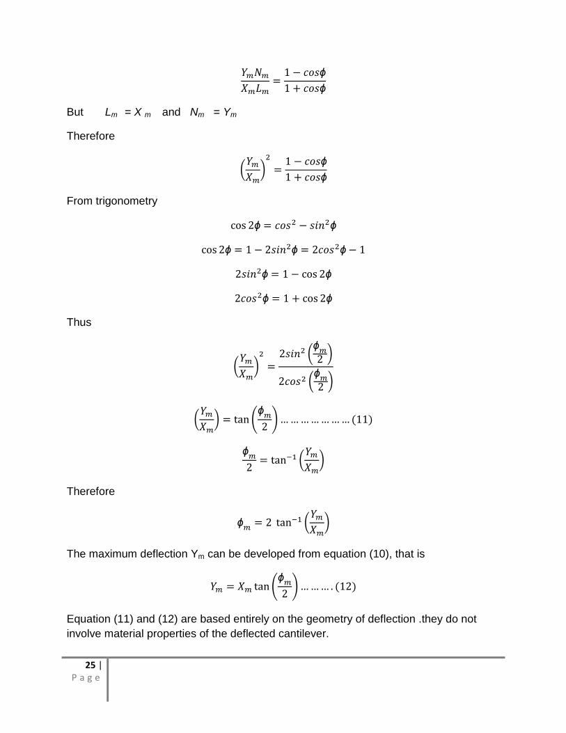
25 | P a g e
But Lm = X m and Nm = Ym
Therefore
From trigonometry
Thus
Therefore
The maximum deflection Ym can be developed from equation (10), that is
Equation (11) and (12) are based entirely on the geometry of deflection .they do not
involve material properties of the deflected cantilever.
26 | P a g e
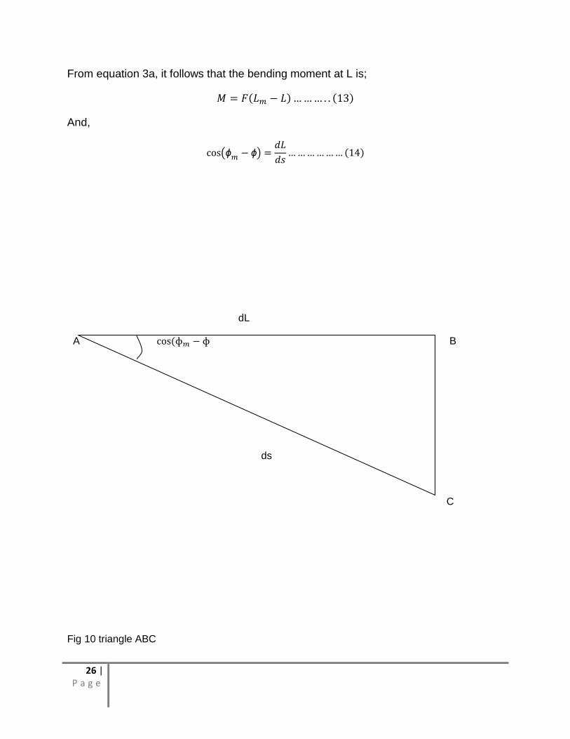
From equation 3a, it follows that the bending moment at L is;
And,
dL
A B
ds
C
Fig 10 triangle ABC
27 | P a g e
Combining equations (1)(13)and (14), it follows that,
But
Hence
Rearranging gives,
Cos (
The introduction of L as the variable of integration instead of s, greatly simplifies the
problem. Equation (15) can be integrated if the relationship between EI and L is known.
The following assumptions may be made as a matter of investigations.
The product EI does not vary with L since ɸ=0 when L=0.
By integrating equation (15) we get;
28 | P a g e
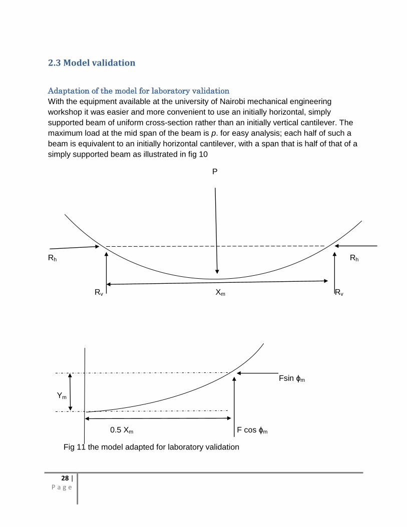
2.3 Model validation
Adaptation of the model for laboratory validation
With the equipment available at the university of Nairobi mechanical engineering
workshop it was easier and more convenient to use an initially horizontal, simply
supported beam of uniform cross-section rather than an initially vertical cantilever. The
maximum load at the mid span of the beam is p. for easy analysis; each half of such a
beam is equivalent to an initially horizontal cantilever, with a span that is half of that of a
simply supported beam as illustrated in fig 10
P
Rh Rh
Rv Xm Rv
Fsin ɸm
Ym
0.5 Xm F cos ɸm
Fig 11 the model adapted for laboratory validation
29 | P a g e
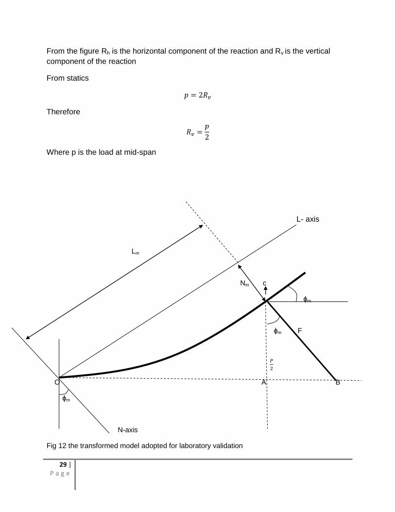
From the figure Rh is the horizontal component of the reaction and Rv is the vertical
component of the reaction
From statics
Therefore
Where p is the load at mid-span
L- axis
Lm
Nm c
ɸm
ɸm F
O A B
ɸm
N-axis
Fig 12 the transformed model adopted for laboratory validation
30 | P a g e
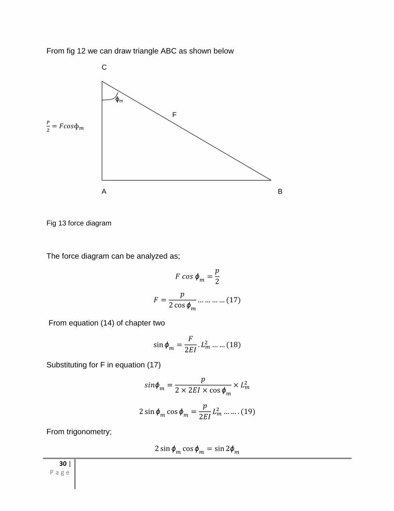
From fig 12 we can draw triangle ABC as shown below
C
ɸm
F
A B
Fig 13 force diagram
The force diagram can be analyzed as;
From equation (14) of chapter two
Substituting for F in equation (17)
From trigonometry;
31 | P a g e
Substituting this into the equation (19), we get
Now, in accordance with equation (3c) of chapter two, it follows from fig 10 and 11 that
And
Substituting equation (21), for Lm into equation (20), we get;
The experimental results were also in agreement with the predictions of the theory from
equation (12) below
Therefore, it follows from equation (22)
Dividing through by 4 gives
Substituting the value of
from equation (23) into equation (12) gives
The above equation was used to validate the model.
32 | P a g e
CHAPTER THREE
3.0 A DESCRIPTION OF APPARATUS USED.
3.1 HAND TOOLS
3.1.1 TAPE MEASURE
A tape measure was used to measure the dimensions of the aluminium specimen.
3.1.2 STEEL RULE
The steel rule was used in measuring the dimensions of the aluminium bar, aiding in
drawing straight lines on the bar and as a straight guide for marking with the scriber.
3.1.3 VERNIER CALIPERS
The vernier calipers was used to measure the thickness of the beam specimen, the
diameter of the rollers and the measurement of the length x.
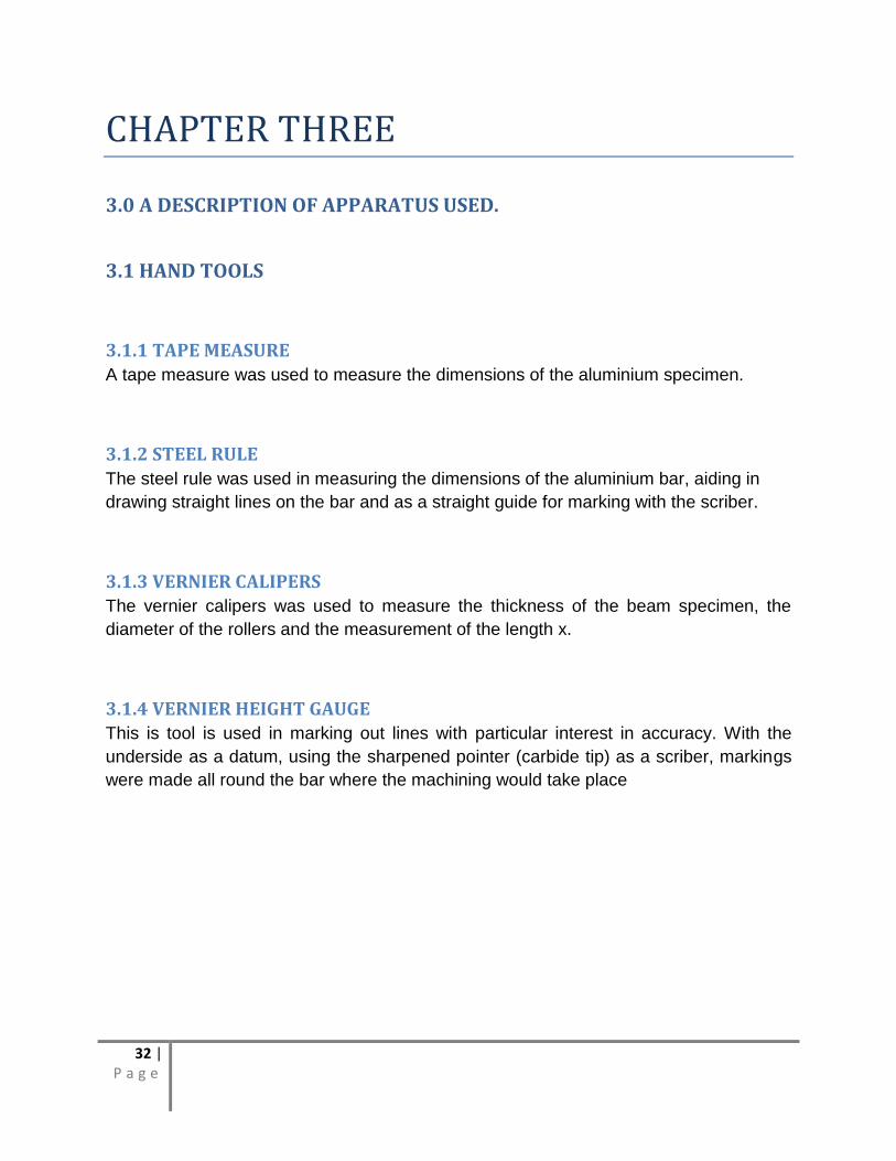
3.1.4 VERNIER HEIGHT GAUGE
This is tool is used in marking out lines with particular interest in accuracy. With the
underside as a datum, using the sharpened pointer (carbide tip) as a scriber, markings
were made all round the bar where the machining would take place
33 | P a g e
Picture 1 vernier height gauge
3.1.5 TRY-SQUARE
The try square was for marking and measuring the aluminium work piece. It was also
used to check the straightness to the adjoining surface.
3.1.6 DIAL GAUGE
The dial gauge was used to measure the deflection of the aluminium specimen when a
load was applied. The mounting of the dial gauge was done in such a way that the dial
gauge sensor was perpendicular to the specimen axis.
3.1.7 ROUGH AND SMOOTH FILE
The hand files were to make smooth the edge of the aluminium specimen after
machining.
3.1.8 SPIRIT LEVEL
The spirit level was used on the specimen to check whether it was level.
34 | P a g e
3.1.9 SCRIBER
A scriber was used in conjunction with the rule and the try square to obtain thin semi-
permanent lines where they were required for machining of the specimen.
3.2 MACHINES
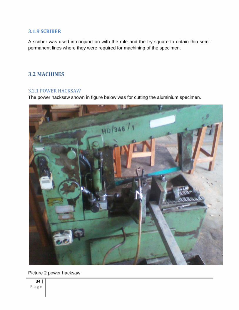
3.2.1 POWER HACKSAW The power hacksaw shown in figure below was for cutting the aluminium specimen.
Picture 2 power hacksaw
35 | P a g e
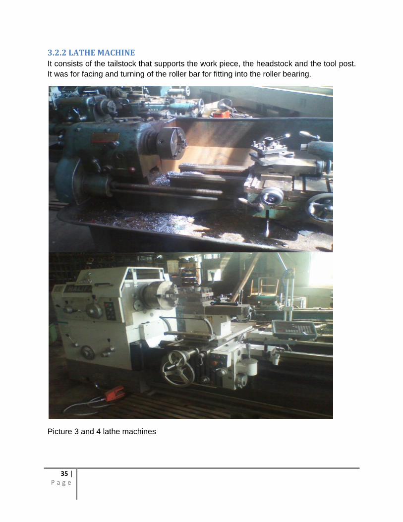
3.2.2 LATHE MACHINE
It consists of the tailstock that supports the work piece, the headstock and the tool post.
It was for facing and turning of the roller bar for fitting into the roller bearing.
Picture 3 and 4 lathe machines
36 | P a g e
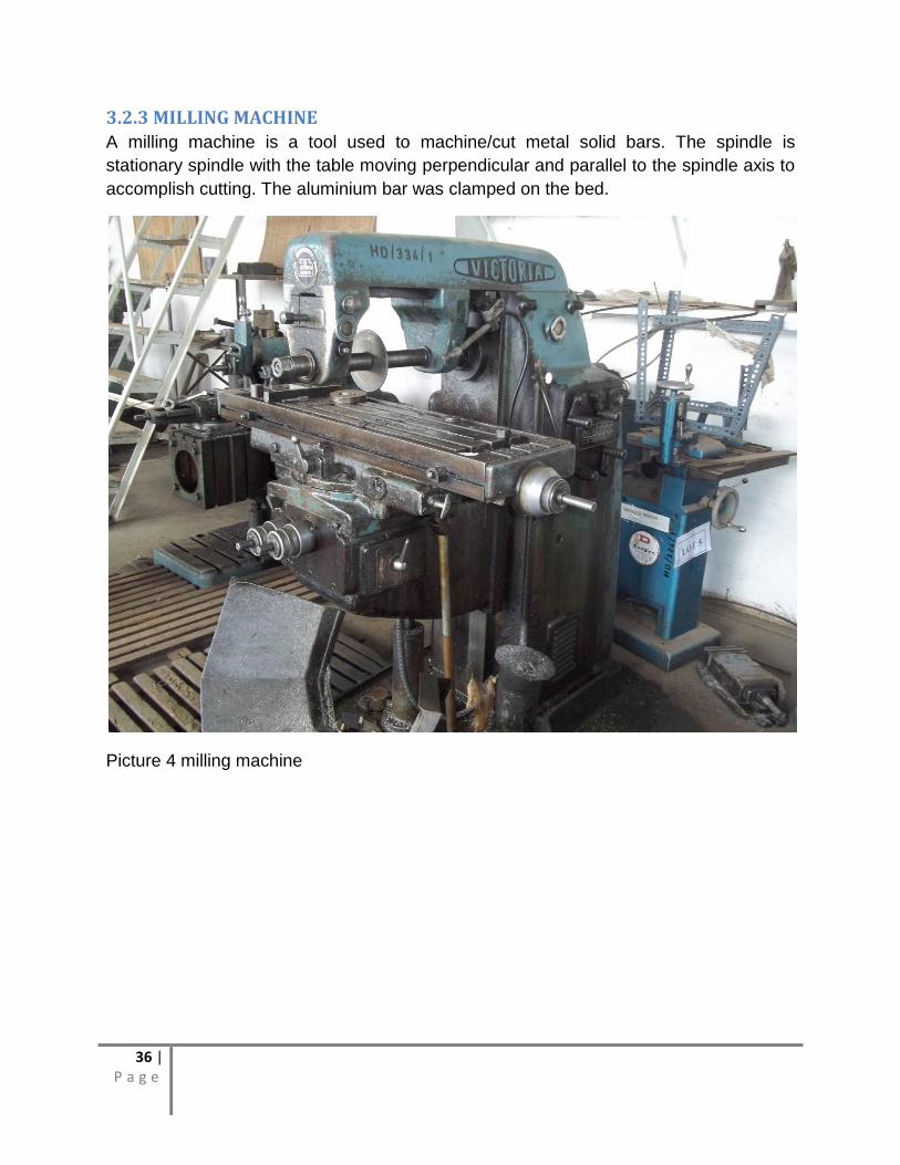
3.2.3 MILLING MACHINE
A milling machine is a tool used to machine/cut metal solid bars. The spindle is
stationary spindle with the table moving perpendicular and parallel to the spindle axis to
accomplish cutting. The aluminium bar was clamped on the bed.
Picture 4 milling machine
37 | P a g e
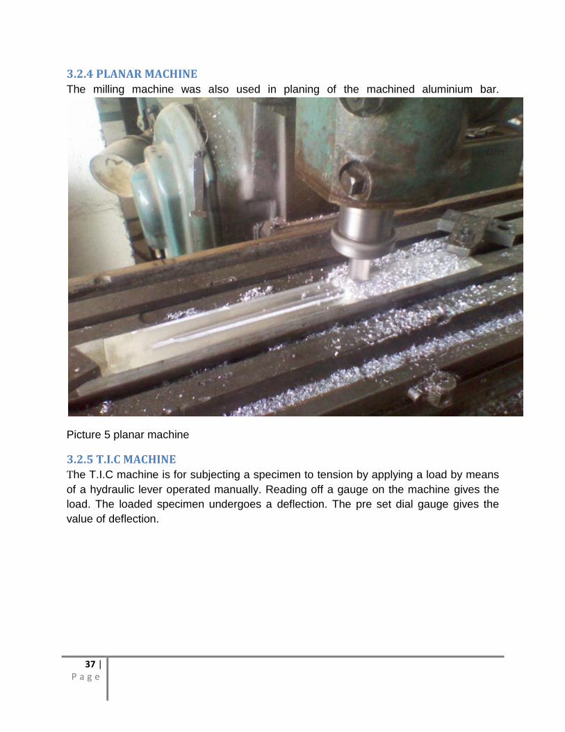
3.2.4 PLANAR MACHINE
The milling machine was also used in planing of the machined aluminium bar.
Picture 5 planar machine
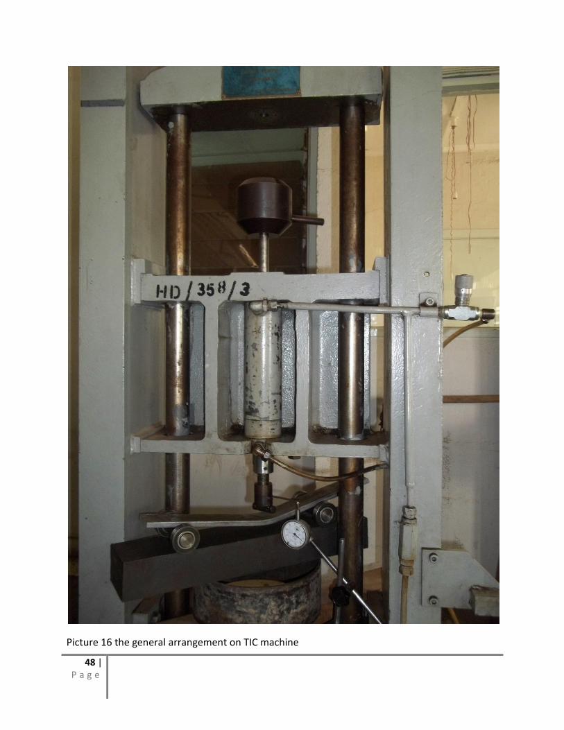
3.2.5 T.I.C MACHINE
The T.I.C machine is for subjecting a specimen to tension by applying a load by means
of a hydraulic lever operated manually. Reading off a gauge on the machine gives the
load. The loaded specimen undergoes a deflection. The pre set dial gauge gives the
value of deflection.
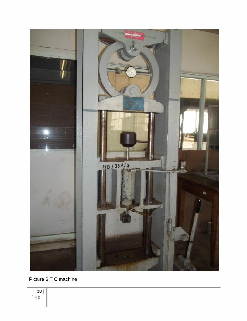
38 | P a g e
Picture 6 TIC machine
39 | P a g e
CHAPTER FOUR
4.0 LABORATORY DATA ACQUISITION
4.1 PREPARATION OF SPECIMEN
4.1.1 PROCEDURE OF PREPARATION
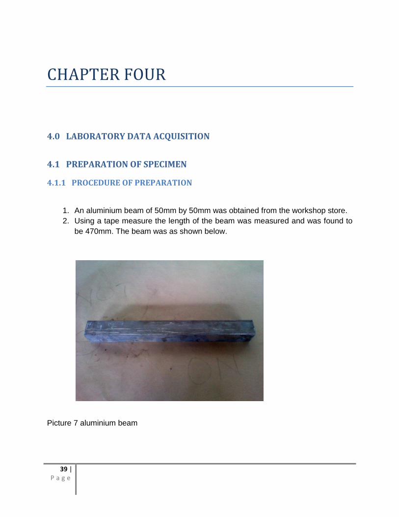
1. An aluminium beam of 50mm by 50mm was obtained from the workshop store.
2. Using a tape measure the length of the beam was measured and was found to
be 470mm. The beam was as shown below.
Picture 7 aluminium beam
40 | P a g e
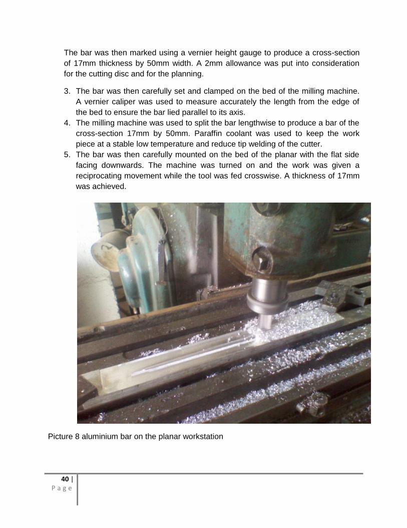
The bar was then marked using a vernier height gauge to produce a cross-section
of 17mm thickness by 50mm width. A 2mm allowance was put into consideration
for the cutting disc and for the planning.
3. The bar was then carefully set and clamped on the bed of the milling machine.
A vernier caliper was used to measure accurately the length from the edge of
the bed to ensure the bar lied parallel to its axis.
4. The milling machine was used to split the bar lengthwise to produce a bar of the
cross-section 17mm by 50mm. Paraffin coolant was used to keep the work
piece at a stable low temperature and reduce tip welding of the cutter.
5. The bar was then carefully mounted on the bed of the planar with the flat side
facing downwards. The machine was turned on and the work was given a
reciprocating movement while the tool was fed crosswise. A thickness of 17mm
was achieved.
Picture 8 aluminium bar on the planar workstation
41 | P a g e
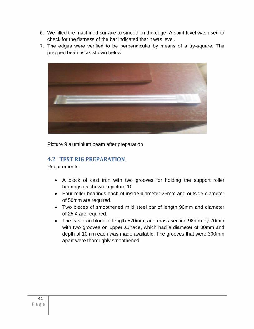
6. We filled the machined surface to smoothen the edge. A spirit level was used to
check for the flatness of the bar indicated that it was level.
7. The edges were verified to be perpendicular by means of a try-square. The
prepped beam is as shown below.
Picture 9 aluminium beam after preparation
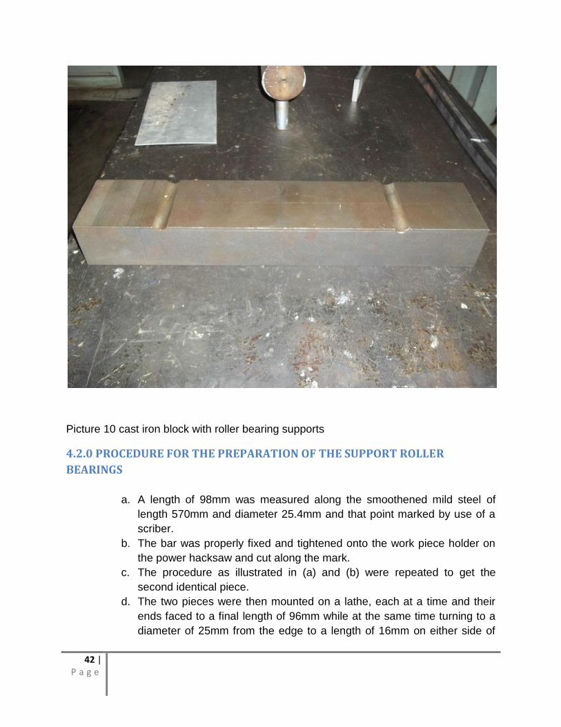
4.2 TEST RIG PREPARATION.
Requirements:
A block of cast iron with two grooves for holding the support roller
bearings as shown in picture 10
Four roller bearings each of inside diameter 25mm and outside diameter
of 50mm are required.
Two pieces of smoothened mild steel bar of length 96mm and diameter
of 25.4 are required.
The cast iron block of length 520mm, and cross section 98mm by 70mm
with two grooves on upper surface, which had a diameter of 30mm and
depth of 10mm each was made available. The grooves that were 300mm
apart were thoroughly smoothened.
42 | P a g e
Picture 10 cast iron block with roller bearing supports
4.2.0 PROCEDURE FOR THE PREPARATION OF THE SUPPORT ROLLER
BEARINGS
a. A length of 98mm was measured along the smoothened mild steel of
length 570mm and diameter 25.4mm and that point marked by use of a
scriber.
b. The bar was properly fixed and tightened onto the work piece holder on
the power hacksaw and cut along the mark.
c. The procedure as illustrated in (a) and (b) were repeated to get the
second identical piece.
d. The two pieces were then mounted on a lathe, each at a time and their
ends faced to a final length of 96mm while at the same time turning to a
diameter of 25mm from the edge to a length of 16mm on either side of
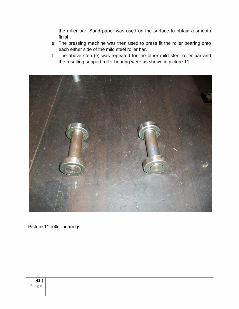
43 | P a g e
the roller bar. Sand paper was used on the surface to obtain a smooth
finish.
e. The pressing machine was then used to press fit the roller bearing onto
each either side of the mild steel roller bar.
f. The above step (e) was repeated for the other mild steel roller bar and
the resulting support roller bearing were as shown in picture 11
Picture 11 roller bearings
44 | P a g e
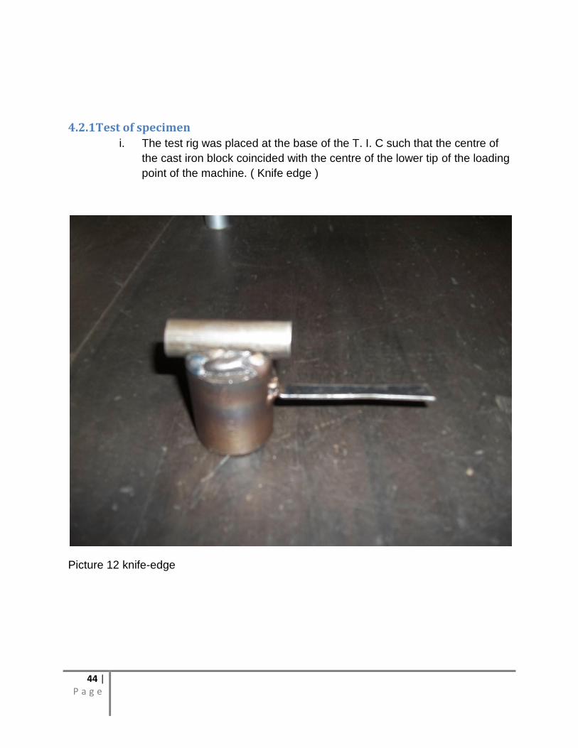
4.2.1Test of specimen
i. The test rig was placed at the base of the T. I. C such that the centre of
the cast iron block coincided with the centre of the lower tip of the loading
point of the machine. ( Knife edge )
Picture 12 knife-edge
45 | P a g e
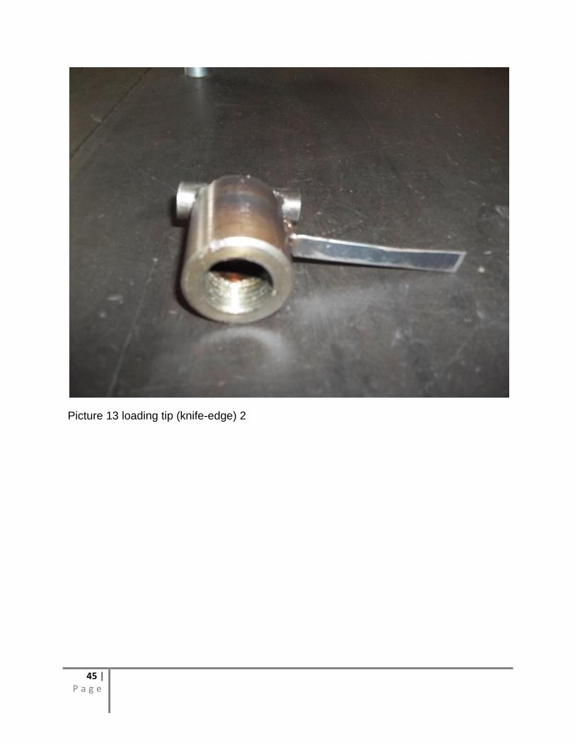
Picture 13 loading tip (knife-edge) 2
46 | P a g e
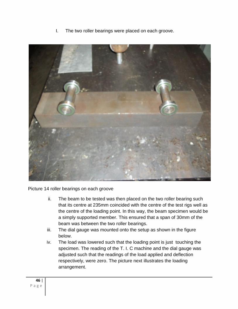
I. The two roller bearings were placed on each groove.
Picture 14 roller bearings on each groove
ii. The beam to be tested was then placed on the two roller bearing such
that its centre at 235mm coincided with the centre of the test rigs well as
the centre of the loading point. In this way, the beam specimen would be
a simply supported member. This ensured that a span of 30mm of the
beam was between the two roller bearings.
iii. The dial gauge was mounted onto the setup as shown in the figure
below.
iv. The load was lowered such that the loading point is just touching the
specimen. The reading of the T. I. C machine and the dial gauge was
adjusted such that the readings of the load applied and deflection
respectively, were zero. The picture next illustrates the loading
arrangement.
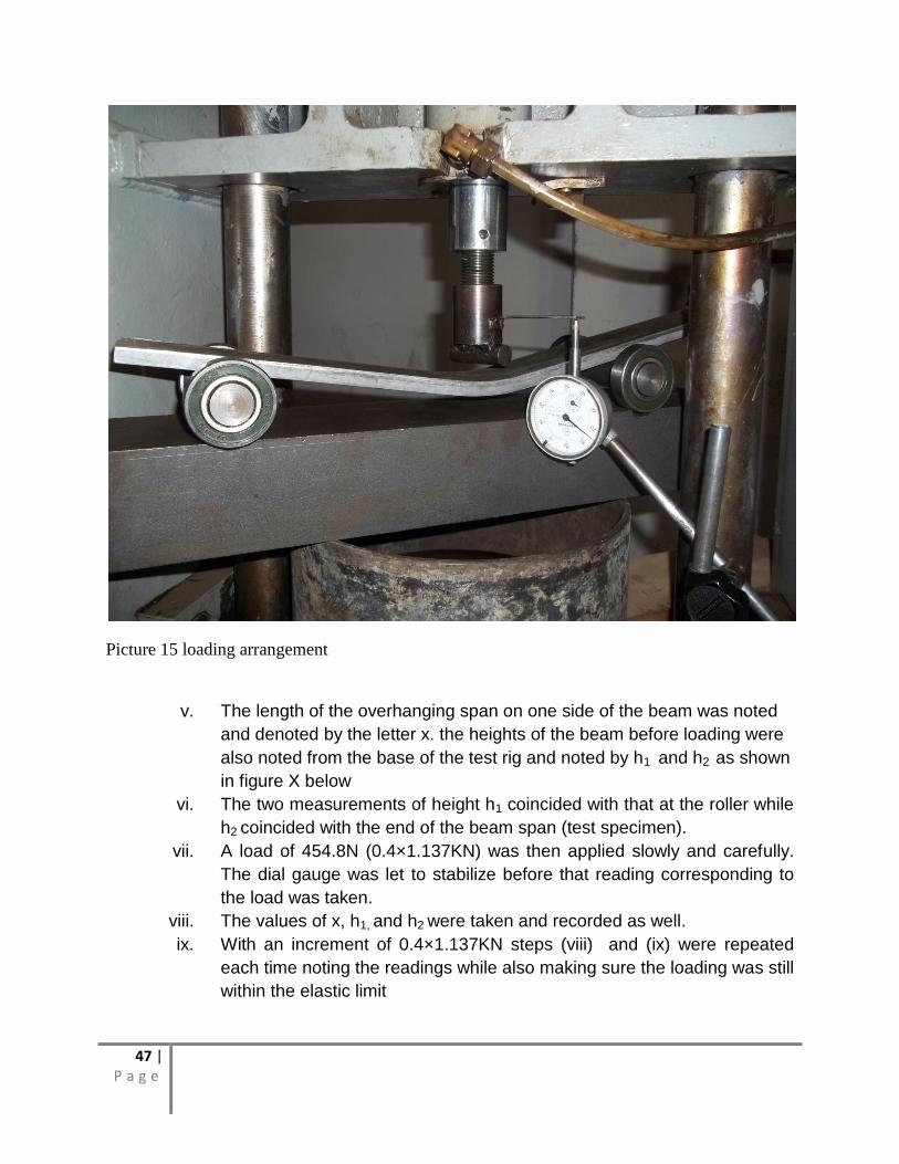
47 | P a g e
Picture 15 loading arrangement
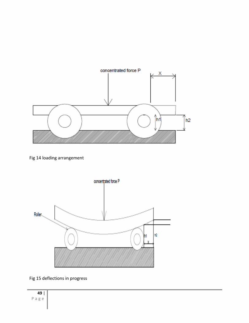
v. The length of the overhanging span on one side of the beam was noted
and denoted by the letter x. the heights of the beam before loading were
also noted from the base of the test rig and noted by h1 and h2 as shown
in figure X below
vi. The two measurements of height h1 coincided with that at the roller while
h2 coincided with the end of the beam span (test specimen).
vii. A load of 454.8N (0.4×1.137KN) was then applied slowly and carefully.
The dial gauge was let to stabilize before that reading corresponding to
the load was taken.
viii. The values of x, h1, and h2 were taken and recorded as well.
ix. With an increment of 0.4×1.137KN steps (viii) and (ix) were repeated
each time noting the readings while also making sure the loading was still
within the elastic limit
48 | P a g e
Picture 16 the general arrangement on TIC machine
49 | P a g e
Fig 14 loading arrangement
Fig 15 deflections in progress

50 | P a g e
Chapter five
Analysis of experimental results
The test was carried out using T.I.C machine found in the strength of materials
laboratory of the University of Nairobi, department of mechanical and manufacturing
engineering workshop. After a series of preliminary tests on the specimens, finally
stable results were recorded in the tables that follow.
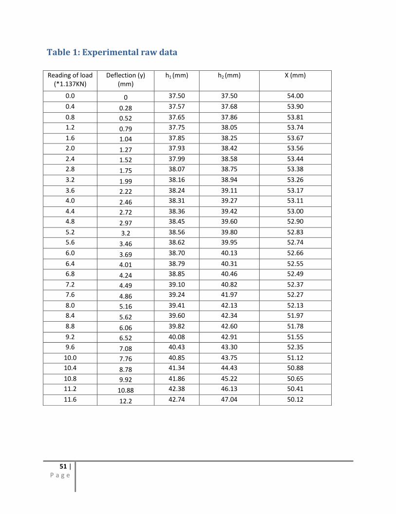
We recorded the exact values of load and deflections as shown in table 2.
51 | P a g e
Table 1: Experimental raw data
Reading of load (*1.137KN)
Deflection (y) (mm)
h1 (mm) h2 (mm) X (mm)
0.0 0 37.50 37.50 54.00
0.4 0.28 37.57 37.68 53.90
0.8 0.52 37.65 37.86 53.81
1.2 0.79 37.75 38.05 53.74
1.6 1.04 37.85 38.25 53.67
2.0 1.27 37.93 38.42 53.56
2.4 1.52 37.99 38.58 53.44
2.8 1.75 38.07 38.75 53.38
3.2 1.99 38.16 38.94 53.26
3.6 2.22 38.24 39.11 53.17
4.0 2.46 38.31 39.27 53.11
4.4 2.72 38.36 39.42 53.00
4.8 2.97 38.45 39.60 52.90
5.2 3.2 38.56 39.80 52.83
5.6 3.46 38.62 39.95 52.74
6.0 3.69 38.70 40.13 52.66
6.4 4.01 38.79 40.31 52.55
6.8 4.24 38.85 40.46 52.49
7.2 4.49 39.10 40.82 52.37
7.6 4.86 39.24 41.97 52.27
8.0 5.16 39.41 42.13 52.13
8.4 5.62 39.60 42.34 51.97
8.8 6.06 39.82 42.60 51.78
9.2 6.52 40.08 42.91 51.55
9.6 7.08 40.43 43.30 52.35
10.0 7.76 40.85 43.75 51.12
10.4 8.78 41.34 44.43 50.88
10.8 9.92 41.86 45.22 50.65
11.2 10.88 42.38 46.13 50.41
11.6 12.2 42.74 47.04 50.12
52 | P a g e
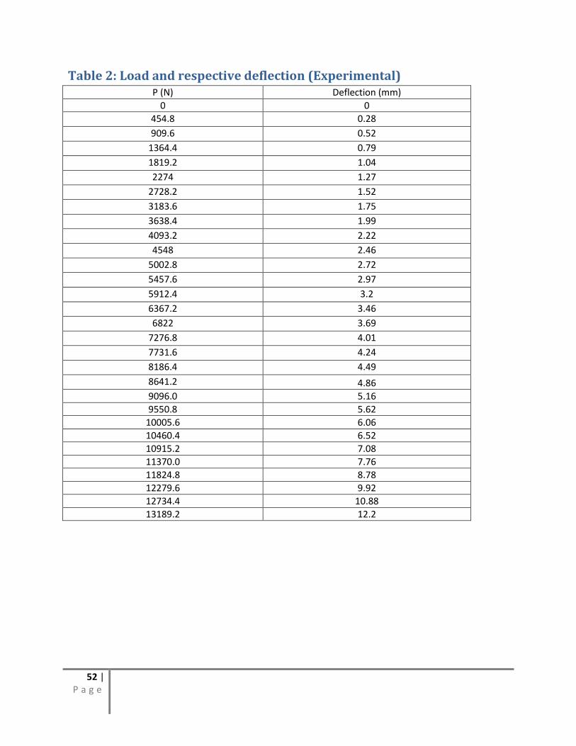
Table 2: Load and respective deflection (Experimental) P (N) Deflection (mm)
0 0
454.8 0.28
909.6 0.52
1364.4 0.79
1819.2 1.04
2274 1.27
2728.2 1.52
3183.6 1.75
3638.4 1.99
4093.2 2.22
4548 2.46
5002.8 2.72
5457.6 2.97
5912.4 3.2
6367.2 3.46
6822 3.69
7276.8 4.01
7731.6 4.24
8186.4 4.49
8641.2 4.86
9096.0 5.16
9550.8 5.62
10005.6 6.06
10460.4 6.52
10915.2 7.08
11370.0 7.76
11824.8 8.78
12279.6 9.92
12734.4 10.88
13189.2 12.2
53 | P a g e
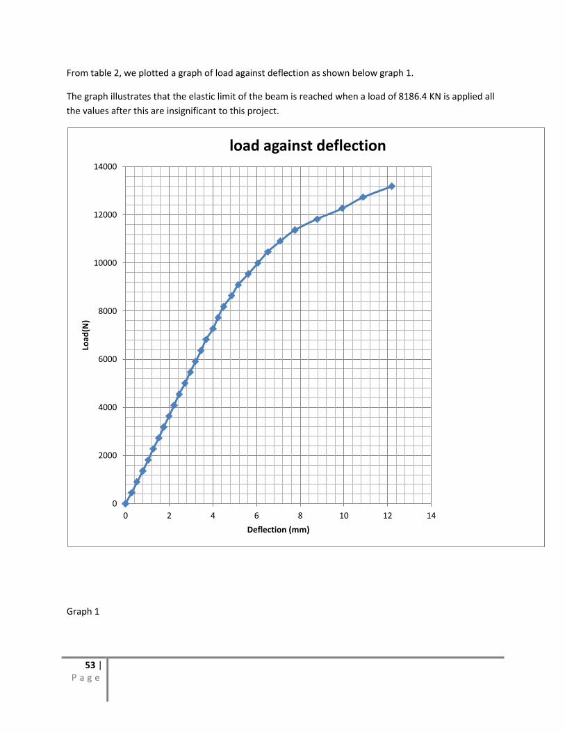
From table 2, we plotted a graph of load against deflection as shown below graph 1.
The graph illustrates that the elastic limit of the beam is reached when a load of 8186.4 KN is applied all
the values after this are insignificant to this project.
Graph 1
0
2000
4000
6000
8000
10000
12000
14000
0 2 4 6 8 10 12 14
Load
(N)
Deflection (mm)
load against deflection
54 | P a g e
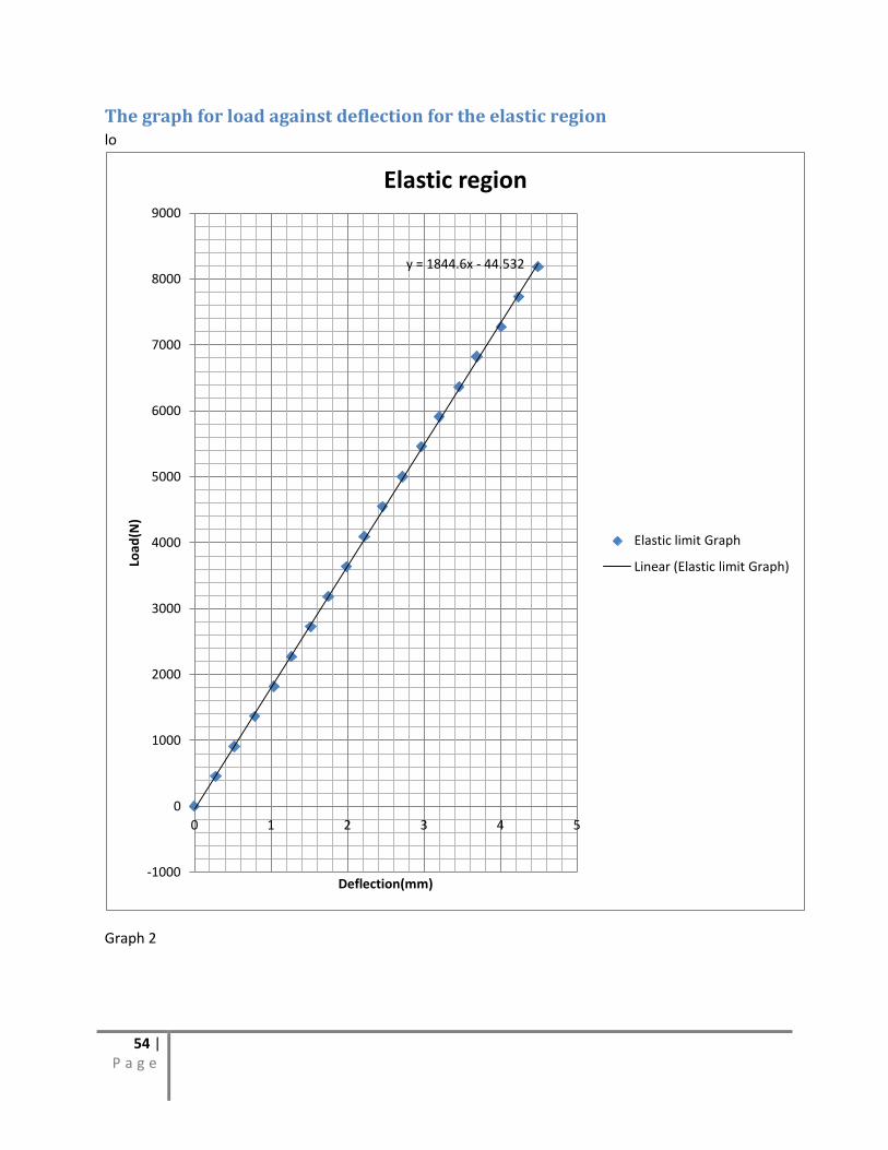
The graph for load against deflection for the elastic region lo
Graph 2
y = 1844.6x - 44.532
-1000
0
1000
2000
3000
4000
5000
6000
7000
8000
9000
0 1 2 3 4 5
Load
(N)
Deflection(mm)
Elastic region
Elastic limit Graph
Linear (Elastic limit Graph)
55 | P a g e
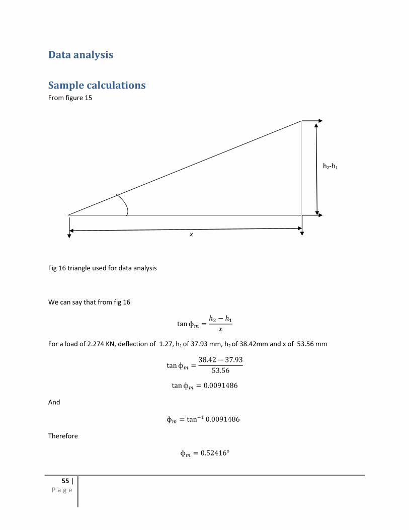
Data analysis
Sample calculations From figure 15
h2-h1
x
Fig 16 triangle used for data analysis
We can say that from fig 16
For a load of 2.274 KN, deflection of 1.27, h1 of 37.93 mm, h2 of 38.42mm and x of 53.56 mm
And
Therefore
56 | P a g e
Hence
We calculated the value of the right hand term of equation (22) using the above values as;
For P=2.274 KN
E = 70 × 109 NM-2
Where
E is young’s modulus of aluminium
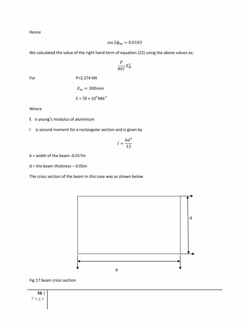
I is second moment for a rectangular section and is given by
b = width of the beam -0.017m
d = the beam thickness – 0.05m
The cross section of the beam in this case was as shown below
d
b
Fig 17 beam cross section
57 | P a g e
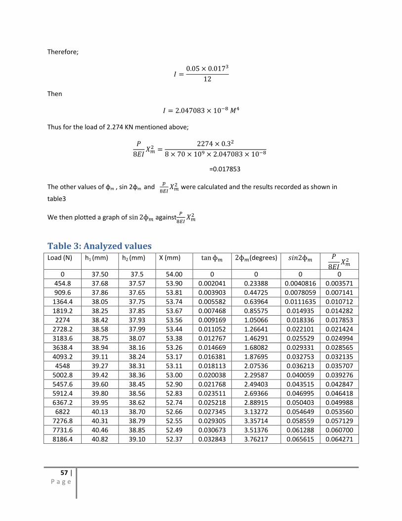
Therefore;
Then
Thus for the load of 2.274 KN mentioned above;
=0.017853
The other values of ɸm , sin 2ɸm and
were calculated and the results recorded as shown in
table3
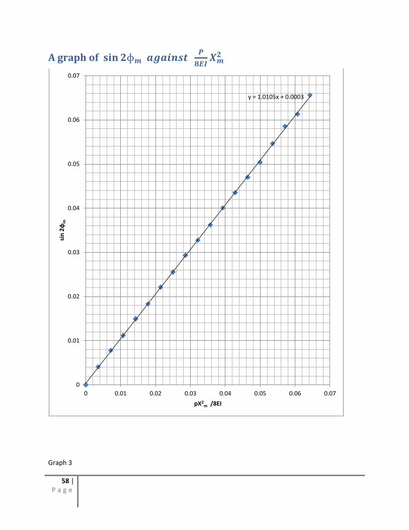
We then plotted a graph of against
Table 3: Analyzed values Load (N) h1 (mm) h2 (mm) X (mm) (degrees)
0 37.50 37.5 54.00 0 0 0 0
454.8 37.68 37.57 53.90 0.002041 0.23388 0.0040816 0.003571
909.6 37.86 37.65 53.81 0.003903 0.44725 0.0078059 0.007141
1364.4 38.05 37.75 53.74 0.005582 0.63964 0.0111635 0.010712
1819.2 38.25 37.85 53.67 0.007468 0.85575 0.014935 0.014282
2274 38.42 37.93 53.56 0.009169 1.05066 0.018336 0.017853
2728.2 38.58 37.99 53.44 0.011052 1.26641 0.022101 0.021424
3183.6 38.75 38.07 53.38 0.012767 1.46291 0.025529 0.024994
3638.4 38.94 38.16 53.26 0.014669 1.68082 0.029331 0.028565
4093.2 39.11 38.24 53.17 0.016381 1.87695 0.032753 0.032135
4548 39.27 38.31 53.11 0.018113 2.07536 0.036213 0.035707
5002.8 39.42 38.36 53.00 0.020038 2.29587 0.040059 0.039276
5457.6 39.60 38.45 52.90 0.021768 2.49403 0.043515 0.042847
5912.4 39.80 38.56 52.83 0.023511 2.69366 0.046995 0.046418
6367.2 39.95 38.62 52.74 0.025218 2.88915 0.050403 0.049988
6822 40.13 38.70 52.66 0.027345 3.13272 0.054649 0.053560
7276.8 40.31 38.79 52.55 0.029305 3.35714 0.058559 0.057129
7731.6 40.46 38.85 52.49 0.030673 3.51376 0.061288 0.060700
8186.4 40.82 39.10 52.37 0.032843 3.76217 0.065615 0.064271
58 | P a g e
A graph of
Graph 3
y = 1.0105x + 0.0003
0
0.01
0.02
0.03
0.04
0.05
0.06
0.07
0 0.01 0.02 0.03 0.04 0.05 0.06 0.07
sin
2ɸ
m
pX2m /8EI
59 | P a g e
More sample calculations
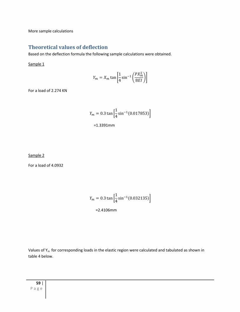
Theoretical values of deflection Based on the deflection formula the following sample calculations were obtained.
Sample 1
For a load of 2.274 KN
=1.3391mm
Sample 2
For a load of 4.0932
=2.4106mm
Values of Ym for corresponding loads in the elastic region were calculated and tabulated as shown in
table 4 below.
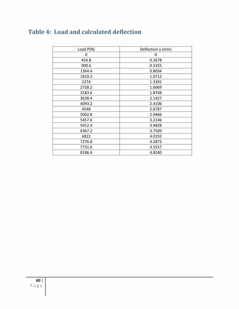
60 | P a g e
Table 4: Load and calculated deflection
Load P(N) Deflection y (mm)
0 0
454.8 0.2678
909.6 0.5355
1364.4 0.8034
1819.2 1.0712
2274 1.3391
2728.2 1.6069
3183.6 1.8748
3638.4 2.1427
4093.2 2.4106
4548 2.6787
5002.8 2.9466
5457.6 3.2146
5912.4 3.4828
6367.2 3.7509
6822 4.0192
7276.8 4.2873
7731.6 4.5557
8186.4 4.8240
61 | P a g e
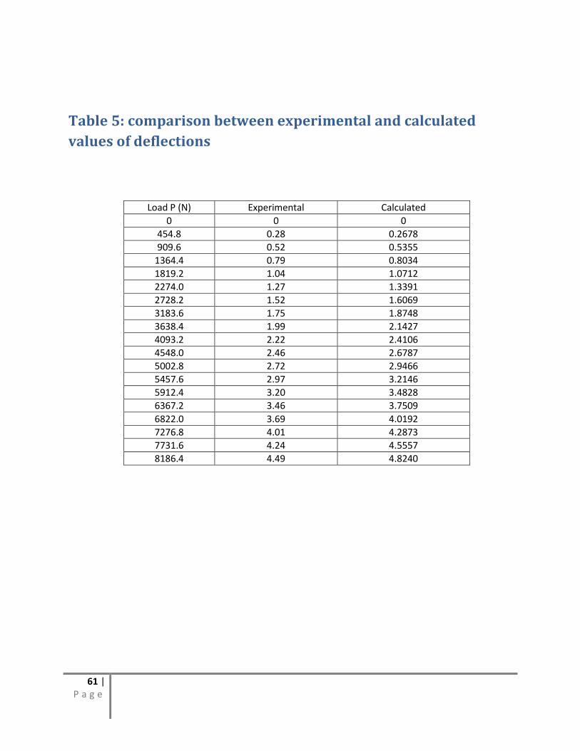
Table 5: comparison between experimental and calculated
values of deflections
Load P (N) Experimental Calculated
0 0 0
454.8 0.28 0.2678
909.6 0.52 0.5355
1364.4 0.79 0.8034
1819.2 1.04 1.0712
2274.0 1.27 1.3391
2728.2 1.52 1.6069
3183.6 1.75 1.8748
3638.4 1.99 2.1427
4093.2 2.22 2.4106
4548.0 2.46 2.6787
5002.8 2.72 2.9466
5457.6 2.97 3.2146
5912.4 3.20 3.4828
6367.2 3.46 3.7509
6822.0 3.69 4.0192
7276.8 4.01 4.2873
7731.6 4.24 4.5557
8186.4 4.49 4.8240
62 | P a g e
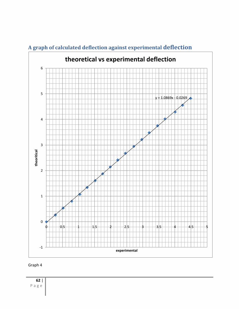
A graph of calculated deflection against experimental deflection
Graph 4
y = 1.0869x - 0.0269
-1
0
1
2
3
4
5
6
0 0.5 1 1.5 2 2.5 3 3.5 4 4.5 5
the
ori
tica
l
experimental
theoretical vs experimental deflection
63 | P a g e
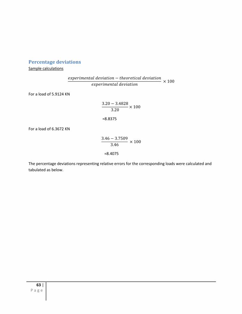
Percentage deviations Sample calculations
For a load of 5.9124 KN
=8.8375
For a load of 6.3672 KN
=8.4075
The percentage deviations representing relative errors for the corresponding loads were calculated and
tabulated as below.
64 | P a g e
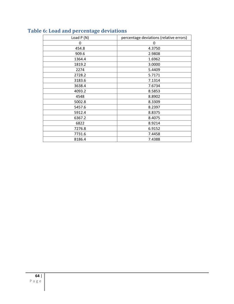
Table 6: Load and percentage deviations Load P (N) percentage deviations (relative errors)
0 0
454.8 4.3750
909.6 2.9808
1364.4 1.6962
1819.2 3.0000
2274 5.4409
2728.2 5.7171
3183.6 7.1314
3638.4 7.6734
4093.2 8.5853
4548 8.8902
5002.8 8.3309
5457.6 8.2397
5912.4 8.8375
6367.2 8.4075
6822 8.9214
7276.8 6.9152
7731.6 7.4458
8186.4 7.4388
65 | P a g e
Chapter six
Discussions, conclusions and recommendations
Discussion The results as tabulated were extensively analyzed as shown previously in the previous chapter. The
analysis was restricted to the elastic region before yielding as we had made a prior assumption of linear
elasticity in the project formulation.
To determine the accuracy and the validity of the method of solution proposed in this study an in depth
analysis of experimental and theoretical values was done. We first obtained the results experimentally
of the large deflection of a simply supported beam under the action of a concentrated load P. secondly;
the numerical results are calculated using the proposed theory. Comparison of the two set of values was
then established. The agreement between the values obtained using our numerical method and those
obtained experimentally was good.
The distributed load due to the weight of the beam was considered negligible and therefore was not
used in the analysis. The numerically calculated deflections were obtained using the Oduori’s proposed
method, which is given by the following equation:
Where is the deflection, P is load, E is young’s modulus, I is the second moment of area and is
the mean distance between the roller supports.
Using equation 22,
from which the final large deflections formula for above was
derived, a graph of
was plotted, from the equation, the plotted graph should be
having an expected gradient of 1 in our case it was 1.0105.
Table 1 shows the deflection as a function of the applied load P whereas the table 4 represents the
numerically calculated values with the aid of the numerical equation. We also included the relative error
(percentage) in the values of calculated numerically as compared with the values measured
experimentally. To further the validation, a comparison was done between theoretical and the
experimental deflection then a graph was plotted of calculated against theoretical deflection. The
expected gradient in case of absolute agreement was 1 however the gradient obtained was 1.0869.
66 | P a g e
The comparisons above show there are some errors that were incurred during the experiment that
caused the deviations from theoretical values. These errors could include:
Calculations did not include deflections due to shearing
Possible residual stresses introduced in the aluminium beam during machining while preparing
the specimen. These stresses have an effect of decreasing the buckling load and are caused by
heat and incompatible internal strains
Errors incurred when taking experimental data ( ), taking the beam dimensions
There was some play encountered from the dial gauge that was used to obtain deflection
The T.I.C machine could not handle heavy tensions and started leaking at high values of load
Young’s modulus for Aluminium varies from 65 GPa to 75 GPa, for the purposes of evaluation 70
GPa was used as the average which may have been inaccurate.
Conclusion The study was a success. The laboratory validation of the new theory (Oduori’s formulae) for
determination of large deflections for a class of cantilever beams by laboratory experimentation was
carried out to satisfaction and found to hold.
The theoretical analysis resulted in the following deflection equation corresponding to the general case
of large deflections.
And as shown in chapter 2 this equation is directly derived from equation 22 as quoted below.
From values of
a linear graph through the origin with a gradient of
1.662 against the expected gradient of 1. The variation occurred because of the experimental errors
It can be concluded that the theory as proposed by professor Oduori is valid for linear analysis of large
deflections of cantilever beams

67 | P a g e
Recommendations for further work We recommend further work to prove this theory based on better experimentation methods and
equipment. There should be extra vigilance to avoid the errors mentioned before. The following should
be taken into consideration
Shear deflections should be incorporated.
The measurement of should be done with extra caution. Using a vernier as we did
introduces errors and it is extremely hard to obtain exact values.
The beam should be prepared using standard preparation methods and its properties like
young’s modulus should be gauged properly. Dimensional in accuracies should also be avoided.
The experiment could be done using a more reliable loading system other than the TIC
machines.
68 | P a g e
Chapter 7 References
B. Shvartsman, large deflections of a cantilever beam subjected to a follower force’, J. Sound and
Vib.304, pp.969-973 (2007) .
F.V. Rhode, ` Large deflections of cantilever beams with uniformly distributed load’, Q. Appl. Math. ,
11, pp. 337-338 (1953)
J. M Gere, S.P .Timoshenko, `Mechanics of materials, second edition’, books Engineering Division,
California (1984)
M.F Oduori, J. Sakai, E. Inoue, `A paper on Modeling of crop stem Deflection in the context of the
combine harvester reel design and operation.
J. Case, C. Lord, and Carl T.F.R., `Strength of materials and structures , fourth edition chapter 13,
deflections of beams,’
S.W. Crawley, R.M. Dillon steel buildings analysis and design, second edition’, chapter 4, beam
deflections
Wikipedia: http://en.wikipedia.org/wiki/Timoshenko beam theory
Wikipedia: http://en.wikipedia.org/wiki/Euler-Bernoulli beam theory
Wikipedia: http://en.wikipedia.org/wiki/Moment area method beam theory