Declaration of own work (Research dissertation)

This thesis has been submitted in fulfilment of the requirements for a postgraduate degree

(e.g. PhD, MPhil, DClinPsychol) at the University of Edinburgh. Please note the following

terms and conditions of use:

This work is protected by copyright and other intellectual property rights, which are

retained by the thesis author, unless otherwise stated.

A copy can be downloaded for personal non-commercial research or study, without

prior permission or charge.

This thesis cannot be reproduced or quoted extensively from without first obtaining

permission in writing from the author.

The content must not be changed in any way or sold commercially in any format or

medium without the formal permission of the author.

When referring to this work, full bibliographic details including the author, title,

awarding institution and date of the thesis must be given.

I

Declaration of own work (Research dissertation).

Full Name ……………………………………………………

Matriculation Number…………………………………………

I hereby declare that this dissertation was composed by me and is my original work and that this work

has not been submitted for any other degree or professional qualification.

Signature ………………………………………………………

Date ……………………………………………………………

II

Acknowledgements.

First and foremost, I would like to thank God Almighty for the gift of life and for the strength to carry

on.

Words cannot express my sincere gratitude to my principal supervisor Dr Craig Watkins, for his

invaluable teaching skills, support, advice, instructions, corrections and patience despite his very busy

schedule. You are an inspiration to me and indeed a role model.

I would also like to thank Dr Andrew Free, for always taking his time to run data and to teach me

what the data is trying to say. I appreciate all the time and sacrifices you have made. My appreciation

also goes to Dr Dave Bartley, for all his professional advice and comforting words that prevented me

from pressing the panic button. My sincere gratitude also goes to my programme coordinator Dr Kim

Picozzi for always been there and for showing great concern regarding the progress of my work.

I also want to thank Dr Karen Stevenson, Dr Val hughes, Alison Morrison, Joyce McLuckie, Fiona

Strathdee for their professional advice and support. My sincere appreciation also goes to Miriam

Navarro and Jelena Nikolic for their most precious roles in previous sample collections and their

excellent DNA extraction skills.

Thanks to all my colleagues not forgetting Anan Ibrahim and Elena Perez for their wonderful

computer skills and their friendship.

To my very lovely wife for supporting me in all areas, for taking care of our children while I was

away in the lab at the Moredun, for allowing me to do full time programme while she did the running

around and taking care of the children, you have shown me the true meaning of love and what

marriage is all about, you are always cherished and appreciated, thank you so very much. To Shiloh

and David, this is dedicated to you, I love you guys very much.

III

List of Abbreviations.

ANOVA Analysis of variance

DNA Deoxyribonucleic acid

dsDNA Double stranded deoxyribonucleic acid

EDTA Ethylenedeminetetracetic acid.

IRT Inhibitor Removal Technology

MAP Mycobacterium avium subspecies paratuberculosis

MRI Moredun Research Institute

NMDS Non metric multidimensional scaling

OTU Operational taxonomic units

PCR Polymerase chain reaction

PERMANOVA Permutational analysis of variance

PERMDISP Permutational multivariate dispersion

PRIMER Plymouth routines in multivariate ecological research

QIIME Quantitative insight into microbial ecology

1

Table of Contents

Declaration…………………………………………………………………………………………………………………………..i

Acknowledgements…………………………………………………………………………………………………………….ii

List of Abbreviations……………………………………………………………………………………………………………iii

1. Abstract ........................................................................................................................ 4

2. Introduction ......................................................................................................................... 5

2.1. Mycobacterium avium subspecies paratuberculosis (MAP). ................................... 5

2.2. Johne’s Disease ........................................................................................................ 6

2.3. Crohn’s Disease. ....................................................................................................... 8

2.4. Parasite vectors and MAP. ....................................................................................... 8

2.5. Gastrointestinal microbiome and the host. ............................................................. 9

2.6 Areas of further Study. ..................................................................................................... 11

3. Methodology .............................................................................................................. 13

3.1 Rectal faecal sample collection ........................................................................................ 13

3.2 Collection and storage of sheep faecal samples .............................................................. 13

3.3 Extraction of DNA from ovine faecal samples. ................................................................ 14

3.4 Quantification and quality control of DNA using Nano drop. .......................................... 15

3.5 Bacterial and Archaeal amplification technique. ............................................................. 15

3.6 Agarose gel electrophoresis. ............................................................................................ 16

3.7 DNA Purification from gel. ............................................................................................... 17

3.8 Quantifluor® One dsDNA System. .................................................................................... 18

3.9 Next Generation Sequencing (Illumina MiSeq). ............................................................... 19

3.9.1 QIIME ............................................................................................................................ 19

3.9.2 Statistical analysis ......................................................................................................... 20

4. Results ........................................................................................................................ 22

4.1 DNA Extraction ................................................................................................................. 22

2

4.2 Polymerase Chain Reaction (PCR). ................................................................................... 25

4.2.1 Gel purified PCR products (DNA) ready for sequencing. ............................................. 27

4.3 Analysis of Bacterial and Archael community. ................................................................. 31

4.4 QIIME Taxonomy Results. ................................................................................................ 32

4.4.1 Taxonomy summary (Phylum level). ............................................................................. 35

4.4.2 Taxonomy Summary (Order level). ............................................................................... 39

43

4.4.3 Taxonomy summary of different groups based on anthelminthic drug used for

Treatment. ............................................................................................................................. 44

55

4.4.4 Taxonomy Summary Genus level. ................................................................................. 56

4.5 Rarefaction Curves. .......................................................................................................... 89

4.6 Shannon – diversity Index ................................................................................................ 91

4.7 Metric Multidimensional Scaling Analysis. ...................................................................... 93

............................................................................................................................................... 98

4.7.1 Statistical View of Outliers at Order level. .................................................................... 99

4.7.2 Statistical view of outliers at Genus level of Taxonomy. ............................................ 102

4.8 MAP and round worm dual infected group (Year 1 collection, Year 2 collection and Year

3 collection). ......................................................................................................................... 110

4.8.1 Analysis of Bacterial and archael community. ............................................................ 113

4.8.2 QIIME Taxonomy Results ............................................................................................ 113

............................................................................................................................................. 147

4.8.4 Shannon Diversity – Index .......................................................................................... 150

4.8.5 Non – Metric Multidimensional Scaling. ..................................................................... 152

4.8.6 Statistical View of Outliers at Order level. .................................................................. 156

4.8.7 Statistical view of outliers at Genus level. .................................................................. 162

4.9 MDS plot for Study 1 and Study 2. ................................................................................. 172

5. DISCUSSION ...................................................................................................................... 175

5.1 Gastrointestinal Microbiome ......................................................................................... 175

3

5.2 Helminth infected group ................................................................................................ 176

5.2.1 Pre- treatment and Post – treated groups based on anthelminthic. ......................... 177

5.2.2 Pre – treatment outliers compared to group 1, group2 and group 3. ........................ 179

5.3 MAP and round worm dual infected group (Year 1 collection, Year 2 and Year 3

collection. ............................................................................................................................. 180

5.3.1 Year 3 collection outliers compared to Year 1 and Year 2. ......................................... 182

5.4 Overall comparison of study 1 and study 2. .................................................................. 183

6. Conclusion. ....................................................................................................................... 184

References. .......................................................................................................................... 185

Appendix A ........................................................................................................................... 188

4

1. Abstract The gastrointestinal microbiome plays an invaluable role in the maintenance and wellbeing

of their host. They are important in the development of host immunity and host digestion.

Despite their vital importance, there is still much to be known about their role in the host and

their diversity during bacterial and parasitic infections.

In the first part of this study, we examined the gut microbiome of 40 sheep (gimmers)

infected only with gastrointestinal nematodes. Rectal faecal samples were taken before

treatment and after treatment with anthelminthic. In the second part of the study, a total of

125 rectal faecal samples were collected from a sheep flock infected with Mycobacterium

avium subspecies paratuberculosis and nematodes. Bacterial DNA was isolated from all

rectal faecal samples using the MOBIO PowerFecal® DNA Isolation Kit.

The faecal samples acted as a surrogate to the gastrointestinal microbiota. Bacterial and

archaeal ecosystems were examined by sequencing the 16sRNA gene V4 amplicons

employing the Illumina sequencing platform. Raw sequenced data was then analysed by the

use of QIIME (Quantitative Insight into Microbial Ecology) with the assigning of taxonomy

to the raw sequenced data and the determination of diversity within the samples. Statistical

analysis was carried out using PRIMER (Plymouth Routine into Microbial Ecological

Research). PERMANOVA and PERMDISP statistical tools were used to analyse the

multivariate data.

In the first part of the study with the nematode only infected sheep, we discovered that the

gastrointestinal microbiome of sheep before and after treatment showed few differences

(P>0.05). This suggest that anthelminthic treatment did not have much effect on the bacterial

and archaeal community in the gastrointestinal tract.

In the second part of the study with the MAP and helminth infected sheep, it was discovered

that the Year 3 samples differ from the Year 2 and Year 1 samples with a P value of 0.001,

suggesting that the progression of disease alters the gastrointestinal microbiome of sheep.

5

2. Introduction

2.1. Mycobacterium avium subspecies paratuberculosis (MAP). Mycobacterium avium subspecies paratuberculosis is a member of the family

Mycobactericeae which are gram positive, acid – fast organisms ((Harris, 2001)). Other

members of significant pathogenic importance include Mycobacterium tuberculosis and

Mycobacterium leprae (Wayne, and Kubica, 1986).

MAP is an obligate intracellular organism of about 0.5 µm by 1.2 µm in size ((El-Zaatari,

2004). It was first identified in Germany by Professor Johne and Dr Frothingham in 1894 as

the causative agent of a severe gastroenteritis of ruminants. The disease was subsequently

called Johne’s disease after its founder ((Singh et al., 2013). It has also been associated with

Crohn’s disease in humans making it a pathogen of zoonotic importance ((Grant, 2005).

MAP is a very slow growing bacteria that depends on the ferric iron extraction ability of

mycobactin to grow on media due to its fastidious nutritional requirement (Sweeney, 1996).

MAP has about 14 to 18 copies of IS900 inserted in its genome. This property is used to

detect MAP by targeting the IS900 which results in more sensitive detection or diagnosis

than targeting a single copy marker (Kim et al., 2004). Research has shown that other

mycobacteria also possess IS900 like sequences which means that, under certain

circumstances, a more detailed check is needed to confirm the presence of MAP by

molecular methods (Cousins et al., 1999).

MAP is a difficult organism to isolate requiring months or years of incubation before they

become visible to the eye, furthermore many strains cannot be grown at all (El-Zaatari,

2004). MAP can therefore be a difficult organism to culture under conventional laboratory

conditions (El-Zaatari, 2004).

Polymerase chain reaction has been employed due to the limitations of traditional

microbiology techniques in detection and diagnosis of MAP (Khare et al., 2004). The

possible drawback encountered with PCR includes excessive nonspecific DNA which can

be derived from host or other organisms, presence of PCR inhibitors in samples and the

quality of genomic DNA preparation (Khare et al., 2004). Through the development of

molecular biology the sensitivities of IS900 based PCR assays for the isolation of MAP from

faecal and tissues samples have improved over the years enabling enhanced DNA extraction

techniques to employ the use of qPCR assays using primers designed to avoid detection of

environmental bacteria (Windsor, 2015). PCR targeting of IS900 is mostly used for the

identification of MAP, providing the advantage of speed over mycobactin method of

6

identification (Cousins et al., 1999). MAP in liquid cultures from faecal origin and also in

milk have been identified by IS900 PCR (Cousins et al., 1999).

MAP can survive for long periods in the environment ((Singh et al., 2013). It is capable of

slow movement in the soil remaining on grass and pasture resulting in infection when

ingested by grazing animals (Salgado et al., 2011). MAP has an average survival rate of up

to 152 to 246 days in the environment depending on favourable environmental conditions

(Singh et al., 2013). It survives for longer periods in water with water reservoirs playing

significant roles in MAP transmissions or infections on farms (Singh et al., 2013). MAP has

also been cultured in milk of animals both clinically infected and sub - clinically infected

(Grant, 2005). Milk contamination with MAP can be as a result of direct entry of MAP into

the udder or as a result of contamination with infected faeces. Studies carried out on the

effect of pasteurization of milk shows that MAP is more heat – resistant than other

Mycobacteria which pasteurization targets (Mycobacteria bovis) with low amounts of viable

MAP surviving pasteurization procedure ((Grant, 2005).

2.2. Johne’s Disease Johne’s disease also known as Paratuberculosis is a disease of domestic and wild ruminants

caused by Mycobacterium avium subspecies paraturberculosis characterized by chronic

granulomatous gastroenteritis seen mainly in the ileum (Singh et al., 2013). Since the

identification of MAP as the causative agent of Johne’s , the disease has spread to the entire

world particularly in the dairy industries (Windsor, 2015). It is therefore a disease that has a

global distribution, causing serious economic losses in the dairy industry due to falls in milk

production and early culling of cows ((Harris, 2001). Johne’s disease has been reported in

almost every country involved in livestock production and has the laboratory capability to

detect disease in livestock (Khare et al., 2004). It causes a drastic fall in production in all

ruminants causing huge losses for the farmer (Singh et al., 2013). Just like in cattle the

distribution in other ruminants (deer, sheep and goats) is also worldwide (Windsor, 2015).

Johne’s disease infection occurs most commonly during neonatal life via the oral route as a

result of consuming infected material (soil, faeces, MAP infected milk or colostrum) or via

oral contact with contaminated udder or surfaces with faeces ((Arsenault et al., 2014).

Following ingestion, the lymphoid tissue of the intestinal mucosa is the main target of MAP

with the M cells of the Peyer’s patches been the point of entry (Singh et al., 2013). It then

invades intestinal macrophages with the capability of resisting host defence mechanisms and

undergoing multiplication within the macrophages as a result of its ability to prevent

7

activation of macrophages, prevent phagosome acidification and weakening of the

presentation of antigens to the immune cells (Lamont et al., 2012).

In sheep, 2 main pathological forms of the disease are described in animals manifesting

clinical signs, namely (1) the Paucibacillary form which is associated with strong cell –

mediated immunity with the inflammatory infiltrate made up of lymphocytes, small

quantities of macrophages with a very low number of Mycobacteria, (2) Multibacillary form

associated with weak cell – mediated immune response with inflammatory infiltrate

comprising of macrophages packed with numerous Mycobacteria (Dennis, Reddacliff, and

Whittington, 2011).

Gross pathology is observed in the intestine and mesenteric lymph nodes with the intestinal

walls becoming thickened and oedematous with traverse folds seen in the mucosa. Lesions

are also seen in the ileum but can also be observed on any part of the intestinal tract (Dennis,

Reddacliff, and Whittington, 2011).

Clinical signs in cattle are observed 2 to 5 years after initial infection and include

diarrhoea, progressive fall in body weight, general wasting and fall in milk production

(Arsenault et al., 2014). The diarrhoea seen in cattle is most of the time thick containing no

blood, mucus or epithelial debris (Mohana et al., 2015). Weeks after the onset of diarrhoea a

swelling may occur below the jaw (bottle jaw) as a result of blood protein lost from blood

stream to the digestive tract (Mohana et al., 2015). Progression of the disease will lead to

dehydration and severe cachexia (Mohana et al., 2015).

In sheep the primary clinical symptoms are seen as a loss in body condition score (Weight

lost), diarrhoea is only seen in few cases (Windsor, 2015). Anorexia, depression and

diarrhoea may be seen in end stages of the disease in goats (Windsor, 2015).

In small ruminants the most definitive method of diagnosis of paratuberculosis is post

mortem examination with histopathology confirmation, looking for pathological changes, fat

reserve depletion, bowel wall thickening and enlargement of gut associated lymph nodes,

and presence of lymphatic cords on serosa surfaces of ileum and caecum (Windsor, 2015).

Whole live – attenuated and killed MAP vaccines have been used in the past and are still in

continuous use in many countries to control Johne’s disease in livestock (Begg and Griffin,

2005). Existing vaccines decrease mortality and faecal shedding but do not prevent animals

from getting infected (Windsor, 2006).Vaccination is a cost – efficient strategy which

prevents the manifestation of clinical Johne’s disease (Fridriksdottir et al., 2000).

8

Vaccination has been used as a control strategy in many countries with good success

(Fridriksdottir et al., 2000). The main disadvantage is that vaccines used do not differentiate

infected from vaccinated animals thereby interfering with serological diagnosis of Johne’s

disease (Bastida and Juste, 2011). Because of this drawback MAP vaccination may not lead

to the eradication of Johne’s disease and can also interfere with tuberculosis eradication

programs (Bastida andJuste, 2011). Vaccination again in sheep also produces a

granulomatous lesion at the injection site due to the oil – based bacterin vaccines (Bastida

and Juste, 2011).

2.3. Crohn’s Disease. Crohn’s disease is a chronic inflammatory disorder of the gastrointestinal tract of humans

affecting mainly the terminal ileum and the colon (El-Zaatari, 2004). The causative agent of

Crohn’s disease remain a subject of scientific debate with the general believe that the disease

has a complex and multifactorial aetiology (Grant, 2005). Although the aetiological agent of

Crohn’s disease is still debatable, the majority of studies published since the year 2000

points to a higher detection rate of MAP by culture, IS900 PCR or MAP specific antibody

response in patients suffering from Crohn’s disease (Grant, 2005). It has been reported that

around 13 out of 100,000 people in the United Kingdom may be afflicted with Crohn’s

disease with 3000 new cases of Crohn’s disease diagnosed annually in the UK (Grant, 2005).

If MAP plays a role in the pathogenesis of Crohn’s disease then the most likely route of

infection is either food or water born with the most likely culprits been milk (other dairy

products), beef and water (Grant, 2005). Crohn’s disease presents with loss of energy, loss of

weight, night sweats, abdominal pain, and pain in the joints, in severe cases it might present

as an abdominal emergency with peritonitis, perforation of terminal ileum or presenting as

acute appendicitis ((El-Zaatari, 2004)).

2.4. Parasite vectors and MAP. Nematode larvae can become contaminated with MAP serving as vectors for the

transmission of Johne’s disease (Whittington, Lloyd, & Reddacliff, 2001). Nematodes have a

simple life cycle, the nematode egg hatches in faeces, it feeds on bacteria and undergo 2

moults becoming a third stage larvae enclosed within a sheath (Singh et al., 2013). The third

stage larvae are negatively geotrophic but positively phototrophic thereby moving out of

faeces and travelling up blades of vegetation where they are consumed by ruminants

(Soulsby, 1968).

In farm conditions, sheep with the Multibacillary form of MAP infection excrete large

amounts of MAP in their faeces and any nematode larvae developing from egg in the same

9

faeces will become contaminated with MAP (Whittington et al., 2001). Animals showing

clinical signs of Johne’s disease can shed 108

MAP / gram of faeces, the shedding of this

large amount of MAP makes it highly probable that the surface of these nematode larvae can

be become contaminated with MAP (Whittington et al., 2001). The contamination of

nematode larvae by MAP in a real farm environment is highly probable because the same

environmental factors that favour survival of the 3 stage larvae also favour survival of MAP

(Anderson, 1992).

The ability of the larva of Haemonchus contortus, Ostertagia circumcincta and

Trichostrongylus colubriformis to take up MAP has been demonstrated (Whittington et al.,

2001). Nematode larvae serve as a viable means or as mechanical vectors for the

transmission of MAP (Singh et al., 2013). Ingestion of larvae contaminated with MAP will

result in the release of MAP in the lumen of the intestine as the larvae gets rid of its sheath

(Whittington et al., 2001). Moreover the ability of nematode larvae to penetrate mucosa of

the gastrointestinal tract provides an additional route for the delivery of MAP to susceptible

animal tissue which aids in the development of the disease (Whittington et al., 2001).

2.5. Gastrointestinal microbiome and the host. Colonization of the host mammalian gastrointestinal tract begins soon after birth

(Malmuthuge, Griebel, & Guan, 2015). Further exposure of the host to specific microbes will

lead to further colonization of the gastrointestinal tract by more microbes during the animals

life (Malmuthuge et al., 2015). The population or assemblage of these microbes within the

gut and their collective genomes is known as the gastrointestinal microbiome ((McDermott

& Huffnagle, 2014).

A symbiotic relationship exists between the host and the gastrointestinal microbiome where

the host provides the microbes with nourishment and an ecosystem to live whereas the

microbes aid in the development of the host gut mucosa enhancing immunity and also play a

vital role in the digestion of complex plant materials (Leser & Mølbak, 2009).

The immune system of the intestine is predominantly underdeveloped without microbial

activities stimulating it to action (McDermott & Huffnagle, 2014). These microbes play

significant roles in the normal development of the gut associated lymphoid tissues (Peyer’s

patches, crypt patches, and isolated lymphoid follicles), spread of gastrointestinal specific

immune responses and prevention of pathogen colonization (Kamada et al., 2013).

Numerous studies have shown that commensal bacteria can hinder pathogen colonization by

directly competing for limited nutrients within the intestine thereby preventing pathogens

from deriving nourishments (Kamada et al., 2013). A very good example of direct

10

competition for nourishment is seen where Escherichia coli competes with

enterohaemorrhagic E.coli for organic acids, amino acids and other nutrients (Leatham et

al., 2009).

The rumen of ruminants is a complex ecosystem of beneficial microbes (Bacterial, Archaea,

yeast, fungi and protozoa) that aid ruminants to digest plant material into utilizable energy

(Sauer, Marx, & Mattanovich, 2012). The microbial population in the rumen play a very

important role in the establishment and development of microbial fermentation beginning

around 2 or 4 weeks as a result of solid feed consumption (Baldwin and Jesse, 1992). A

complex process of digestion occurs in the rumen as a result of the presence of this vast

assemblage of gastrointestinal microbes which makes it possible for ruminants to utilize

cellulose and other structural and non-structural carbohydrates (Agrawal et al., 2014).

Enzymes needed for the degradation of complex plant materials (polysaccharides) are not

produced by the ruminants themselves but are rather produced by microbes that live in the

rumen ecosystem (Henderson et al., 2015). The resultant fermentation process that occurs

due to the activities of ruminal microbial organisms leads to the production of volatile fatty

acids which serves as a major source of energy (Henderson et al., 2015).

The population of ruminal microbes is usually affected by diet and feeding strategies, but

despite these facts there is a similarity of rumen bacteria found to be abundant in different

parts of the globe (Henderson et al., 2015). The 7 most recognised abundant bacteria include

Prevotella, Butyrivibrio, Ruminococcus, unclassified Lachnospiraceae, Ruminococcaceae,

Bacteroidales and clostridiales, These group of bacteria can be regarded as the core rumen

microbiome because of their presence in a large selection of ruminants (Henderson et al.,

2015). Another group of microbes found in the rumen are the archaea with the majority

being methanogens and the dominant types were found to be similar in all regions of the

world (Henderson et al., 2015). For many rumen bacteria, diet plays a major role in

determining their abundance. Bacteria populations from forage fed animals were discovered

to be similar to each other while bacteria population from concentrate fed animals were also

similar to each other (Henderson et al., 2015).

The gastrointestinal microbiota of humans is composed of trillions of microbes most of

which are non – pathogenic bacteria and viruses (Reyes et al., 2010). The microbiota works

in collaboration with the host immune system to protect the body against pathogen

colonization and invasion. The microbiota also provides essential nutrients and vitamins and

aids in extraction of short chain fatty acids and amino acids from diets. Disturbances in the

microbiota can occur due to exposure to environmental factors such as diet, toxins, drugs and

11

pathogens. Enteric pathogens have the greatest probability to cause dysbiosis in the gut

microbiota.

Crohn’s disease is considered one of the prevalent forms of inflammatory bowel disease

with a characteristic inflammation of the intestinal mucosa (Carding et al., 2015). The

aetiology of Crohn’s disease is still debatable but there is overwhelming evidence that

intestinal microbial dysbiosis plays a major role in its pathogenesis (Baumgart & Carding,

2007). Ultimately patients suffering from Crohn’s disease show a decrease in microbial

population, functional diversity and stability of gut microbiota with specific decrease in

Firmicutes and an accompanying increase in Bacteroidetes and facultative anaerobes such as

Enterobacteriaceae (Hansen, Gulati, & Sartor, 2010).

2.6 Areas of further Study. The need to understand the microbiome of sheep as it relates to Johne’s disease is an area

that will require more studies and research. Is dysbiosis in the gastrointestinal microbiome

responsible for the clinical manifestation of the disease and if dysbiosis plays a role in the

infection what are the factors that trigger this dysbiosis? Further understanding of the role of

the gastrointestinal microbiome and its contribution to the development of the

gastrointestinal tract immune system in ruminants is needed. Quite a number of bacteria,

archaea are found in the rumen and other parts of the gastrointestinal tract of sheep but

which ones are involved in the development of the gastrointestinal immune system and in the

development of the gastrointestinal tract are yet to be identified.

Within the commercial farm environment, there is an association between animals that show

clinical signs of Johne’s disease and also carried high worm burdens. This association might

imply a relationship in which the larvae of the worm act as either a vector carrying MAP on

the surface of its body or inside its body. Further work is needed to establish an

understanding of the relationship between nematodes infestation and MAP infection.

Johne’s disease infection normally occurs early in life, at the neonatal stages in sheep with

disease manifesting after 2 – 4 years, the susceptibility of age to infection is also an area that

needs further investigation in order to establish what role the gastrointestinal microbiome

plays in exposing young animals to infection with MAP and making adult animals more

resistant to the disease.

In this particular project I intend to carry out an analytical study to understand the

relationship between Johne’s disease pathogenesis, gastrointestinal microbiome and

gastrointestinal parasites. Initially, I will investigate the role of the gut microbiome and

intestinal parasites. This will be followed by investigating the dual infection of intestinal

parasites in association with the clinically affected Johne’s diseased sheep from a

12

commercially run farm with a known history of MAP infection. By comparing these two

studies, the unique bacterial flora that is associated with dual infections in sheep can be

analysed.

The eventual aim of this project is to identify biomarkers that could be used in an improved

diagnostic test and develop preventative control strategies that can be used to improve the

wellbeing of livestock by manipulation of the gut flora using dietary supplements or

probiotics to inhibit the colonisation of the gut with MAP. Probiotics can be used for

regulating the equilibrium and activities of the gastrointestinal microbiome (Uyeno,

Shigemori, and Shimosato, 2015)

13

3. Methodology

3.1 Rectal faecal sample collection Rectal faecal samples of sheep (Scottish black face, gimmers) were collected as surrogate

samples for the small intestine content from 9 commercial farms without a history of Johne’s

disease. They were divided into groups depending on which anthelminthic treatment they

received: (following manufacturer’s dose rate per kilogram body weight) as below:

Group 1 - Zolvix® (2.5mg kg bodyweight of Monenpantel)

Group 2 - Startect ® (2mg Derquantel and 0.2mg Abamectin per kg bodyweight)

Group 3 – Zolvix® + Startect®

After 14 days faecal samples were taken from each sheep and frozen at -80°C

All the faecal samples taken from each sheep were frozen at -80°C.

This research was also part of a larger project to assess the impact of single or sequential

administration of the two new anthelmintic compounds (Zolvix® and/or Startect®) and to

determine if the sequential administration of the two new active drenches (Zolvix® and

Startect®) has an additive/synergistic or antagonistic effect using animals sourced from a

number of farms. Faecal samples obtained from Day 0 and Day 14 were stored at -80oC to

determine if differences in treatment had an effect on the faecal microbiome of sheep in each

treatment group pre and post treatment.

3.2 Collection and storage of sheep faecal samples Ovine faecal samples were collected from 2 farms with Scottish black face breed of sheep

with a history of Johne’s disease and gastro-intestinal nematodes. Samples were collected

once annually for a period of 3 years (Year 1 collection, Year 2 collection and Year 3

collection). The faecal samples were collected from the rectum and immediately packaged in

plastic bags labelled with the sheep number, before being placed in a cold box and

transported to the Moredun Research Institute where they were sorted and placed in the -

80°C storage freezers.

Blood samples were also taken intravenously through the jugular vein. The blood samples

were collected in vacutainer tubes and stored in cold boxes and then transported to the

Moredun Research Institute for storage and subsequent forwarding to BioBest Laboratories

for analysis for the presence of serum antibody using a commercial ELISA test (Appendix

A).

14

3.3 Extraction of DNA from ovine faecal samples. Microbial DNA was extracted from sheep faecal samples using MO BIO PowerFecal®

DNA Isolation Kit by carefully following the manufacturer’s extraction instructions. 0.25

grams of faecal sample were loaded into 2 ml tubes containing dry beads (provided in the

kit). 750µl of Bead Solution was added to each tube. The faeces within the tubes were

homogenized by vortexing for 10 seconds. 60µl of Solution C1 containing an anionic

detergent (sodium dodecyl sulphate) was then added to each tube sample and vortexed for 10

seconds. The samples were then heated at 65°c for 10 minutes to further lyse the cells. The

bead tubes were then secured in a horizontal MO BIO Vortex Adapter tube holder and vortex

for 10 minutes at room temperature and afterwards centrifuged at 13000xg for 1 minute to

pellet the cell and faecal debris. Between 400 - 500µl of the supernatant was then transferred

from each tube to a clean 2ml collection tube. Non DNA organic and inorganic materials,

cell debris and protein were precipitated from the supernatant by adding 250µl of solution

C2 which is a patented Inhibitor Removal Technology ® (IRT); a reagent that precipitates

non-DNA organic and inorganic material including polysaccharides, cell debris and proteins.

The mixture was vortexed to mix for 10 seconds then incubated at 4°C for 5 minutes.

Samples were again centrifuged at 13,000xg for 1 minute. About 600µl of the supernatant

were then transferred to clean 2ml collection tubes, carefully avoiding the transfer of the

pelleted material. 200µl Solution C3 was then added to the samples and vortexed before

incubating again at 4°C for 5 minutes. The samples were then centrifuged at 13,000xg for 1

minute. Avoiding the pellet about 750µl of the supernatant was transferred to a clean 2ml

collection tube. Solution C4 (a high salt concentrated solution) was mixed by shaking before

adding 1200µl (C4) to each of the samples to aid in the binding of DNA to the silica within

the spin filters columns provided by the manufacturer. A volume of 650µl of the mixture in

each tube was then loaded into the spin filters and centrifuged at 13000xg for 1 minute. The

flow through was discarded and the process repeated 3 times until all the sample supernatant

was loaded into the spin filters. The spin filter columns were then washed twice with 500µl

of an ethanol based solution C5 to further clean the silica bound DNA by removing residual

salt and contaminants. The spin filters were centrifuged and the flow through discarded.

After the second wash, the spin columns were then carefully placed in 2ml Eppendorf’s

(without covers) and centrifuged at 13,000xg for 5 minutes to further remove the ethanol

from the spin filters. The spin filters were then carefully placed in clean 2ml collection tubes.

100µl of sterile elution buffer C6 (10mM Tris) was carefully added to the centre of the filter

membrane and incubated for 1 minute to ensure the entire membrane was wet enough to

enable a more efficient and complete release of the DNA from the silica filter membrane.

15

The samples were then centrifuged at 13,000xg for 1 minute. The spin filter columns were

then discarded and the eluted DNA was collected and quantified before storage at -20°C.

3.4 Quantification and quality control of DNA using Nano drop. A Spectrophotometer was used to quantify the concentration of nucleic acid in all the

samples extracted. This was done with the NanoDropTM

ND-1000 spectrophotometer

machine (ThermoLabs) using 1.5µl of DNA sample and measuring the nucleic acid

concentration and calculating the purity of the DNA by assessing the 260:280 and 260:230

ratios.

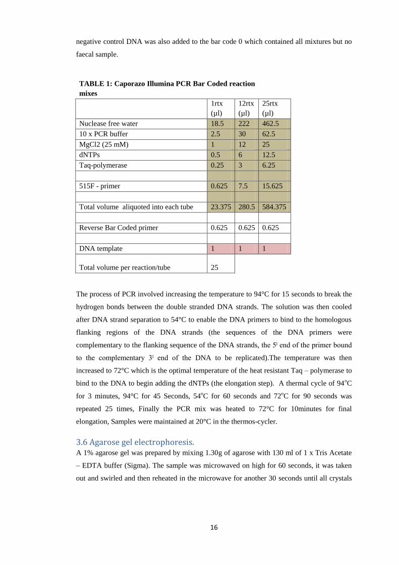
3.5 Bacterial and Archaeal amplification technique. Bacterial and Archaeal DNA were amplified by Illumina bar coded polymerase chain

reaction (PCR) following the method illustrated by Caporazo et al., 2012. This was carried

out in a DNA free PCR preparation room under sterile conditions using Taq DNA

Polymerase dNTPack (ROCHE). A single reaction with a total volume of 25µl composed of

18.5µl nuclease free water, 2.5µl of 10 x PCR buffer, 1µl Magnesium chloride (25 mM),

0.5µl dNTPs (containing four deoxyribonuleotide triphosphate; adenine, guanine, thymine

and cytosine), 0.25µl heat resistant Taq – polymerase (ROCHE) , 0.625µl 515F – forward 5’

primer, 0.625µl reverse barcoded primer and 1µl of DNA template.

Figure 1: 515F primer sequence

5ˡ Illumina adapter Forward pad Forward linker Forward

primer (515F).

The 515F primer is a short sequence of DNA that attaches to the 3ˡ of the flanking region of

the DNA strand .

Figure 2: 806R barcoded reverse primer

Reverse complement of 3ˡ Barcode Reverse Pad Reverse linker Reverse

Primer (806R) Illumina adapter

The reverse bar coded primer is a short sequence of DNA that attaches to the 3ˡ end of the

complementary DNA strand. Master mixes were transferred out of the DNA free room and

1µl of a DNA sample (extracted as described above) was added in each tube. 1µl of the

AATGATACGGCGACCACCGAGATCTACAC TATGGTAATT GT GTGCCAGCMGCCGCGGTAA

CAAGCAGAAGACGGCATACGA

GAT

TCCCTTGTCTC

C

CC GGACTACHVGGGTWTCTAAT AGTCAGTCAG

16

negative control DNA was also added to the bar code 0 which contained all mixtures but no

faecal sample.

TABLE 1: Caporazo Illumina PCR Bar Coded reaction

mixes

1rtx

(µl)

12rtx

(µl)

25rtx

(µl)

Nuclease free water 18.5 222 462.5

10 x PCR buffer 2.5 30 62.5

MgCl2 (25 mM) 1 12 25

dNTPs 0.5 6 12.5

Taq-polymerase 0.25 3 6.25

515F - primer 0.625 7.5 15.625

Total volume aliquoted into each tube 23.375 280.5 584.375

Reverse Bar Coded primer 0.625 0.625 0.625

DNA template 1 1 1

Total volume per reaction/tube 25

The process of PCR involved increasing the temperature to 94°C for 15 seconds to break the

hydrogen bonds between the double stranded DNA strands. The solution was then cooled

after DNA strand separation to 54°C to enable the DNA primers to bind to the homologous

flanking regions of the DNA strands (the sequences of the DNA primers were

complementary to the flanking sequence of the DNA strands, the 5ˡ end of the primer bound

to the complementary 3ˡ end of the DNA to be replicated).The temperature was then

increased to 72°C which is the optimal temperature of the heat resistant Taq – polymerase to

bind to the DNA to begin adding the dNTPs (the elongation step). A thermal cycle of 94oC

for 3 minutes, 94°C for 45 Seconds, 54oC for 60 seconds and 72

oC for 90 seconds was

repeated 25 times, Finally the PCR mix was heated to 72°C for 10minutes for final

elongation, Samples were maintained at 20°C in the thermos-cycler.

3.6 Agarose gel electrophoresis. A 1% agarose gel was prepared by mixing 1.30g of agarose with 130 ml of 1 x Tris Acetate

– EDTA buffer (Sigma). The sample was microwaved on high for 60 seconds, it was taken

out and swirled and then reheated in the microwave for another 30 seconds until all crystals

17

became clear. It was cooled under tap water until hand temperature. 10µl of gel red

(GelRed™ Nucleic acid stain, 10,000x in water) was added and mixed. The mixture was

then poured unto the tray, air bubbles removed; comb was placed and left to stand for about

30 minutes. After verifying that the gel was set, the agarose gel was carefully placed into

electrophoresis machine ensuring that the 1x Tris Acetate - EDTA buffer was at a level just

above the gel. The comb was then removed.

25µl PCR DNA samples were mixed with 5µl of 6x loading dye (Promega), then loaded into

the agarose gel wells starting with the 100bp ladder (Bioline) and then the negative control.

The amplified DNA in all the PCR samples were then separated by size through the process

of electrophoresis. Electrophoresis was run at 100 volts. After 90 minutes it was turned off

and the gel carefully lifted out of the machine. The DNA bands within the gel were

visualised under ultraviolet light and the image of the gel was taken using Alphalmager™

2200 photographic machine.

The appropriately sized DNA band (400bp) on the gel were located and cut out under blue

light using a size 15 scalpel. Each band was placed in a specific marked and identified

collection tube ready for gel purification.

3.7 DNA Purification from gel. DNA was purified from agarose using the Wizard® SV Gel PCR clean – up system,

following the manufacturer’s protocol (Promega). The gel sample in each collection tube

was weighed and Membrane Binding solution was added at a ratio of 10µl per 100mg of

agarose gel slice in each tube. The mixture was vortex and incubated at 65°c for 10 mins

with vortex repeated every 2 minutes. The tubes were then spun in the centrifuge at 16,000xg

for about 2 seconds to remove condensation from the lid of the tubes. The dissolved mixtures

were then transferred to SV mini-columns that were placed in collection tubes and samples

were incubated for one minute, at room temperature. The samples were then centrifuged at

16,000xg for 1 minute. The SV mini-columns were removed from each spin column

assembly, the liquid was discarded, and the SV mini-column returned to the collection tube.

The SV columns were washed by adding 700µl of membrane wash solution and centrifuged

at 16,000xg for 1 minute. The flow through from each column was discarded, and another

700µl of membrane wash solution was again added and centrifuged and the flow through

discarded. SV mini-columns were then placed in 1.5ml Eppendorf’s with no lid and spun for

5 minutes at 16,000xg. The mini-columns were then carefully transferred to clean 1.5ml

micro tube. 50µl of nuclease free water was added directly to the centre of the mini-columns,

18

incubated for 1 minute and then centrifuged for 1 minute at 16000xg. Mini-columns were

then discarded and samples were stored at -20°c.

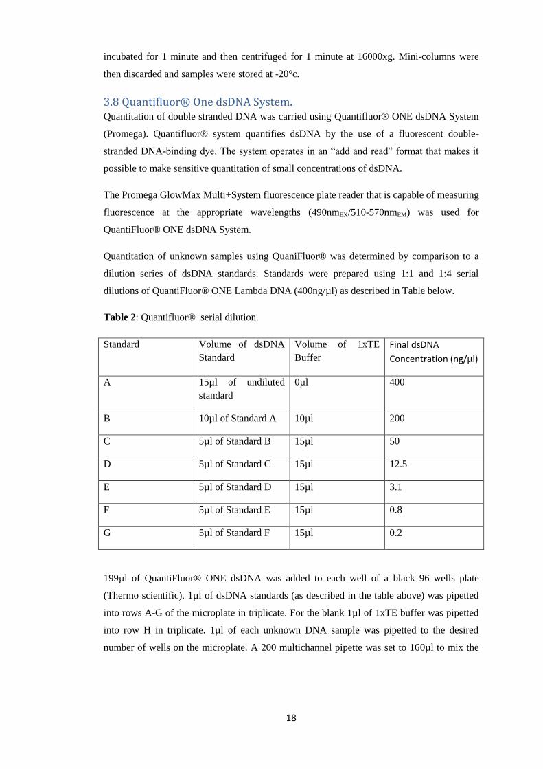
3.8 Quantifluor® One dsDNA System. Quantitation of double stranded DNA was carried using Quantifluor® ONE dsDNA System

(Promega). Quantifluor® system quantifies dsDNA by the use of a fluorescent double-

stranded DNA-binding dye. The system operates in an “add and read” format that makes it

possible to make sensitive quantitation of small concentrations of dsDNA.

The Promega GlowMax Multi+System fluorescence plate reader that is capable of measuring

fluorescence at the appropriate wavelengths (490nmEX/510-570nmEM) was used for

QuantiFluor® ONE dsDNA System.

Quantitation of unknown samples using QuaniFluor® was determined by comparison to a

dilution series of dsDNA standards. Standards were prepared using 1:1 and 1:4 serial

dilutions of QuantiFluor® ONE Lambda DNA (400ng/µl) as described in Table below.

Table 2: Quantifluor® serial dilution.

Standard Volume of dsDNA

Standard

Volume of 1xTE

Buffer

Final dsDNA

Concentration (ng/µl)

A 15µl of undiluted

standard

0µl 400

B 10µl of Standard A 10µl 200

C 5µl of Standard B 15µl 50

D 5µl of Standard C 15µl 12.5

E 5µl of Standard D 15µl 3.1

F 5µl of Standard E 15µl 0.8

G 5µl of Standard F 15µl 0.2

199µl of QuantiFluor® ONE dsDNA was added to each well of a black 96 wells plate

(Thermo scientific). 1µl of dsDNA standards (as described in the table above) was pipetted

into rows A-G of the microplate in triplicate. For the blank 1µl of 1xTE buffer was pipetted

into row H in triplicate. 1µl of each unknown DNA sample was pipetted to the desired

number of wells on the microplate. A 200 multichannel pipette was set to 160µl to mix the

19

content of each well of the plate 3 times by pipetting and ejecting the volume very carefully

and slowly (care was taken to avoid introducing air bubbles during mixing so as to avoid

interference while reading the fluorescence in the GlowMax fluorimeter). The microplate

plate (assay) was incubated for 5 minutes at room temperature protected from light. The

multiwell plate was placed in the GlowMax fluorescence plate reader to measure the

fluorescence ensuring that the Blue Fluorescence OpticaL Kit was inserted into the

GloMax®. The dsDNA concentration was calculated by copying and pasting the raw

fluorescence data into the Promega online tool:

www.promega.com/resources/tools/quantifluordye-systems-data-analysis-workbook

3.9 Next Generation Sequencing (Illumina MiSeq). PCR amplicons were pooled together, ensuring that all samples were equally represented.

These pooled amplicon library was visualised by gel electrophoresis before being taken to

Edinburgh Genomics (University of Edinburgh) for sequencing using the Illumina paired-

end barcoded sequence to identify each sample in the pool. The Illumina MiSeq sequencing

platform was used which employs the use of 3 separate sequencing primers. 2 of the primers

are used to read sequences from the two different ends of the DNA and the third is to

identify the Barcoded sequence unique to each sample.

Figure 3: Illumina MiSeq sequencing primers.

Caporaso Read 1 Primer: Which reads from the 5ˡ end of the amplicon.

Caporaso Read 2 Primer: Which reads from the 3ˡ end of the amplicon

Indexing Primer: Reads the barcode sequence (Caporaso et al., 2010a)

3.9.1 QIIME Quantitative insights into microbial ecology (QIIME) is an open source software pipeline

that analyses and compares microbial community sequence data. QIIME supports a variety

of microbial community analysis and visualization functions. By using QIIME pipeline, raw

sequenced data can be analysed by operational taxonomic picking, taxonomic assignment,

alpha diversity analysis, beta diversity analysis (Caporaso et al., 2010b).

TATGGTAATT GT GTGCCAGCMGCCGCGGTAA

AGTCAGTCAG CC GGACTACHVGGGTWTCTAAT

ATTAGAWACCCBDGTAGTCC GG CTGACTGACT

http://www.promega.com/resources/tools/quantifluordye-systems-data-analysis-workbook

20

Demutiplexed data (grouped into different samples based on barcoded primers) was obtained

from Edinburgh Genomics of the University of Edinburgh. This data was then processed by

using QIIME guard lines as follows:

Pairing of reads (forward and reverse reads) minimum of 200bp. Quality filter (reads shorter

than 400bp of V4 region are filtered out as aborted reads) and combine the paired read files.

The bacterial 16SrRNA V4 region is bigger than 250bp, therefore any short reads that falls

below 250bp were filtered out with Python script. Python script is not part of the standard

QIIME installation but was downloaded from Tony Walter’s website of

https://gist.github.com/walters/7602058. Robert Edgar’s webpage was used to download the

Usearch pipeline that was used for chimera sequences (DNA sequences made up of DNA

from 2 or more parents) using the UCHIME function (Edgar et al., 2011). Approximately 3 –

5% of chimeric sequences were detected in the datasets. These chimeras (DNA sequences

composed of DNA from two or more parents) were then filtered out. De novo operational

taxonomic unit (OTU) picking was carried out clustering similar samples. Sequences that are

at least 97% in resemblance were clustered together and taxonomic assignments of OTUs

against GreenGenes (database for the 16SrRNA gene)13_8 was carried out by Uclust by

clustering sequences that are similar. OTUs were summarized by taxonomic ranking.

Taxonomic levels for the 16SrRNA gene datasets were Phylum, Class, Order, Family and

Genus. Alpha rarefaction curves showing specie richness in each sample and Shannon

diversity that shows specie richness and evenness of distribution of species in the samples

were performed. Singletons OTUs that occur only once in the data set were removed.

3.9.2 Statistical analysis PRIMER (Plymouth Routines in Multivariate Ecological Research) is a worldwide standard

software tool used to analysed the QIIME output data. The OTU tables derived from QIIME

were standardized by dividing each matrix entry by its column total and subsequently

multiplied by 100 to form an impressive display or an orderly arrangement of relative

abundance data. The relative abundance data were imported into Primer 6 version 6.1.12

(Prime – E, Ivybridge, UK).

Bray-Curtis coefficient similarity measure that is particularly common in ecological studies

was used in PRIMER to examine resemblances between samples. A Bray-Curtis similarity of

100 represents 2 communities that are absolutely identical, while a zero Bray-Curtis

similarity coefficient reveals no shared species between samples (Clarke & Warwick, 2001).

https://gist.github.com/walters/7602058

21

Multi-dimensional scaling (MDS) plots were generated from the Bray – Curtis similarity

matrices. Lack of resemblance between samples is shown as distance between points in 2

dimensional plots (Clarke & Warwick, 2001). Kruskal stress value (Kruskal, 1964) was used

to determine the precision of the MDS by the fitting of the various plots into the 2

dimensional plot.

Location and dispersion effects between multivariate samples were analysed by using

PERMANOVA (permutational multivariate analysis of variance) and PERMDISP

(Anderson et al., 2008) with the PERMANOVA + add on package for PRIMER 6.

PERMANOVA engages distance based analysis of the multivariate data in response to

analysis of variance (ANOVA). Permutational multivariate dispersion (PERMDISP) was

used to test the homogeneity of the multivariate dispersions in comparing the beta-diversity

of the samples.

22

4. Results In this study, sheep from a variety of flocks (specified as flock number 1 to 9) were selected

and purchased by Moredun Research Institute (MRI). They were moved to the MRI Firth

Mains farm where they were quarantined. The gimmers (young female sheep) were

individually weighed and the flock split into 3 groups based on the anthelminthic agent used

(Table 1).

Seven days after arrival to Firth Mains, rectal faecal samples were taken from each sheep

and a faecal egg count was carried out to identify the level of worm burdens in the individual

gimmers. The faecal samples were labelled in a bag with the sheep number and date of

collection (07/09/15) and frozen at -80°C. The day of this faecal collection which was also

the day of anthelminthic administration after faecal collection was identified as Day 0.

Table 1: Grouping of gimmers based on anthelminthic treatment after faecal collection.

Sheep Group Anthelminthic

Group 1 Zolvix® (2.5mg per kg bodyweight of monepantel)

Group 2 Startect®(2mg derquantel and 0.2mg abamectin per

kg bodyweight).

Group 3 As above in groups 1 and 2 administered

sequentially.

Day 14:

Fourteen days post treatment, rectal faecal samples were again collected par rectum from

each sheep (gimmer) and frozen at -80°C. Faecal egg counts were carried out in all the

samples to determine the efficacy of the anthelminthic used.

4.1 DNA Extraction

DNA was extracted from the stored faecal samples (-80°C) using the MOBIO PowerFecal®

DNA Isolation kit. The quantity of DNA from each faecal sample collected from both Day 0

and Day 14 was determined (Table 2).

Table 2: Set of DNA samples extracted from rectal samples taken on Day 0 and Day 14

Animal Flock Day 0 Day 14

23

ID Number1 DNA ID DNA

concentration

(ng/µl)

DNA ID DNA

concentration

(ng/µl)

6283 1 DNA 1A7 28.77 DNA 1A21 99.44

6285 1 DNA 1C7 48.96 DNA 1C21 142.92

6289 1 DNA 1D7 25.13 DNA 1D21 112.96

6291 1 DNA 1E7 66.3 DNA 1E21 106.25

6293 1 DNA 1F7 27.8 DNA 1F21 71.88

6295 1 DNA 1G7 56.66 DNA 1G21 81.07

6332 1 DNA 1H7 23.89 DNA 1H21 Not selected

6350 1 DNA 1I7 76.62 DNA 1I21 89.76

6357 1 DNA 1J7 78.42 DNA 1J21 Not selected

6354 1 DNA 1K7 43.4 DNA 1K21 Not selected

334 2 DNA 2A7 109.45 DNA 2A21 Not selected

336 2 DNA 2B7 112.81 DNA 2B21 Not selected

2279 2 DNA 2C7 70.67 DNA 2C21 89.93

2283 2 DNA 2D7 8.81 DNA 2D21 Not selected

2286 2 DNA 2E7 91.94 DNA 2E21 148.53

2287 2 DNA 2F7 100.13 DNA 2F21 91.25

2294 2 DNA 2G 7 113.69 DNA 2G21 98.70

2296 2 DNA 2H7 17.92 DNA 2H21 Not selected

2305 2 DNA 2I7 93.32 DNA 2I21 69.23

2362 2 DNA 2J7 125.29 DNA 2J21 100.76

586 4 DNA 4A7 49.66 DNA 4A21 147.76

587 4 DNA 4B7 56.47 DNA 4B21 104.95

588 4 DNA 4C7 99.5 DNA 4C21 84.90


24

605 4 DNA 4E7 47.77 DNA 4E21 39.75

609 4 DNA 4F7 34.29 DNA 4F21 82.41

610 4 DNA 4G7 99.57 DNA 4G21 10.74

613 4 DNA 4H7 48.49 DNA 4H21 113.94

615 4 DNA 4I7 73.5 DNA 4I21 82.05

625 4 DNA 4K7 46.2 DNA 4K21 71.42

4687 6 DNA 6A7 88.98 DNA 6A21 81.18

4689 6 DNA 6B7 98.59 DNA 6B21 42.55

4720 6 DNA 6C7 60.71 DNA 6C21 70.68


5714 6 DNA 6E7 72.55 DNA 6E21 88.20

5790 6 DNA 6F7 6.64 DNA 6F21 55.55

5798 6 DNA 6G7 14.75 DNA 6G21 Not selected

5908 6 DNA 6I7 90.38 DNA 6I21 Not selected

6005 6 DNA 6J7 86.83 DNA 6J21 Not selected

6011 6 DNA 6K7 49.85 DNA 6K21 Not selected

6014 6 DNA 6L7 72.4 DNA 6L21 Not selected

5323 7 DNA 7A7 114.66 DNA 7A21 Not selected

9715 7 DNA 7B7 28.01 DNA 7B21 Not selected

9718 7 DNA 7C7 10.24 DNA 7C21 Not selected


13813 7 DNA 7E7 85.24 DNA 7E21 Not selected

13816 7 DNA 7F7 107.16 DNA 7F21 75.29

13818 7 DNA 7G7 113.44 DNA 7G21 Not selected

13819 7 DNA 7H7 92.23 DNA 7H21 125.12

13820 7 DNA 7I7 116.58 DNA 7I21 98.27

25

13828 7 DNA 7J7 58.29 DNA 7J21 108.53

2472 8 DNA 8A7 131.99 DNA 8A21 140.66

2474 8 DNA 8B7 116.62 DNA 8B21 116.94

2489 8 DNA 8C7 148.88 DNA 8C21 192.55

3351 8 DNA 8D7 177.36 DNA 8D21 99.62

3494 8 DNA 8E7 112.39 DNA 8E21 217.08

3574 8 DNA 8F7 114.16 DNA 8F21 Not selected

3575 8 DNA 8G7 126.95 DNA 8G21 91.84

3578 8 DNA 8H7 134.82 DNA 8H21 102.51

3587 8 DNA 8I7 19.26 DNA 8I21 156.34

3641 8 DNA 8J7 129.93 DNA 8J21 26.86

1 flock of origin, before transport to MRI Firth Mains Farm

4.2 Polymerase Chain Reaction (PCR). Illumina bar coded PCR (Caporazo et al., 2012) was carried out in pre - treatment and post

treated DNA extracted samples. Pre-treatment DNA samples were assigned barcodes 21 to

60 while post-treated DNA samples were assigned bar codes 61 to 99. Negative control that

is the kit control that had no faecal sample but went through the same process of extraction

and PCR like other samples was assigned a bar code of 0.

26

Figure 1: A representative ultraviolet Image of the PCR results for pre – treatment

samples:

Lane Barcode

100BP BP

1 0

2 21

3 22

4 23

5 24

6 25

7 26

8 27

9 28

10 29

11 30

27

From figure 1, it can be seen that there are no bands in lane 1 which is expected because it is

the well with the negative control BC 0 sample which does not contain any faecal sample.

DNA bands can be seen in all the other lanes except lane 6 which represents the bar coded

PCR product BC 25 from DNA ID 1F7, identified as animal ID 6293. The PCR reaction was

repeated for sample BC 25 at a template concentration of 1:10 which subsequently worked

for this sample

Figure 2: A representative ultraviolet image of the PCR results for post-treated.

From the above picture there is no DNA band in lane 1 which contains the negative control 0

with no faecal sample. There are no bands in lane 3 and lane 7 which contain DNA

amplicons BC 62 and BC 67 respectively. Sample BC 62 and BC 67 were repeated at a

template concentration of 1:10 which subsequently worked for these samples.

4.2.1 Gel purified PCR products (DNA) ready for sequencing. After DNA extraction from the pre-treatment and post treated samples and the amplification

of the 16SrRNA gene V4 using PCR, a total of 38 pre-treated samples and 37 post- treated

samples were gel purified and selected for sequencing. Pre-treatment samples BC46 and

Lane Barcode

BP BP

1 0

2 61

3 62

4 63

5 64

6 65

7 66

8 67

9 68

10 69

11 70

28

BC57 failed after PCR which means their corresponding post-treated samples BC86 and

BC97 were also not selected. Pre-treatment sample BC60 does not have a corresponding

post-treated sample.

Table 3: Pre-treatment and Post treated samples selected for sequencing.

Animal

ID

Flock

ID

DNA

ID

DNA

ng/µl

Bar

Code

DATE

Sample

collected

Additional

Information

6283 1 1A7 28.77 21 07/09/2015 Pre-treatment

6285 1 1C7 48.96 22 07/09/2015 Pre-treatment

6289 1 1D7 25.13 23 07/09/2015 Pre-treatment

6291 1 1E7 66.3 24 07/09/2015 Pre-treatment

6293 1 1F7 27.8 25 07/09/2015 Pre-treatment

6295 1 1G7 56.66 26 07/09/2015 Pre-treatment

6350 1 1I7 76.62 27 07/09/2015 Pre-treatment

2279 3 2C7 70.67 28 07/09/2015 Pre-treatment

2286 3 2E7 91.94 29 07/09/2015 Pre-treatment

2287 3 2F7 100.13 30 07/09/2015 Pre-treatment

2294 3 2G7 113.69 31 07/09/2015 Pre-treatment

2305 3 2I7 93.32 32 07/09/2015 Pre-treatment

2362 3 2J7 125.29 33 07/09/2015 Pre-treatment

586 4 4A7 49.66 34 07/09/2015 Pre-treatment

587 4 4B7 56.47 35 07/09/2015 Pre-treatment

588 4 4C7 99.5 36 07/09/2015 Pre-treatment

605 4 4E7 47.77 37 07/09/2015 Pre-treatment

609 4 4F7 34.29 38 07/09/2015 Pre-treatment

610 4 4G7 99.57 39 07/09/2015 Pre-treatment

613 4 4H7 48.49 40 07/09/2015 Pre-treatment

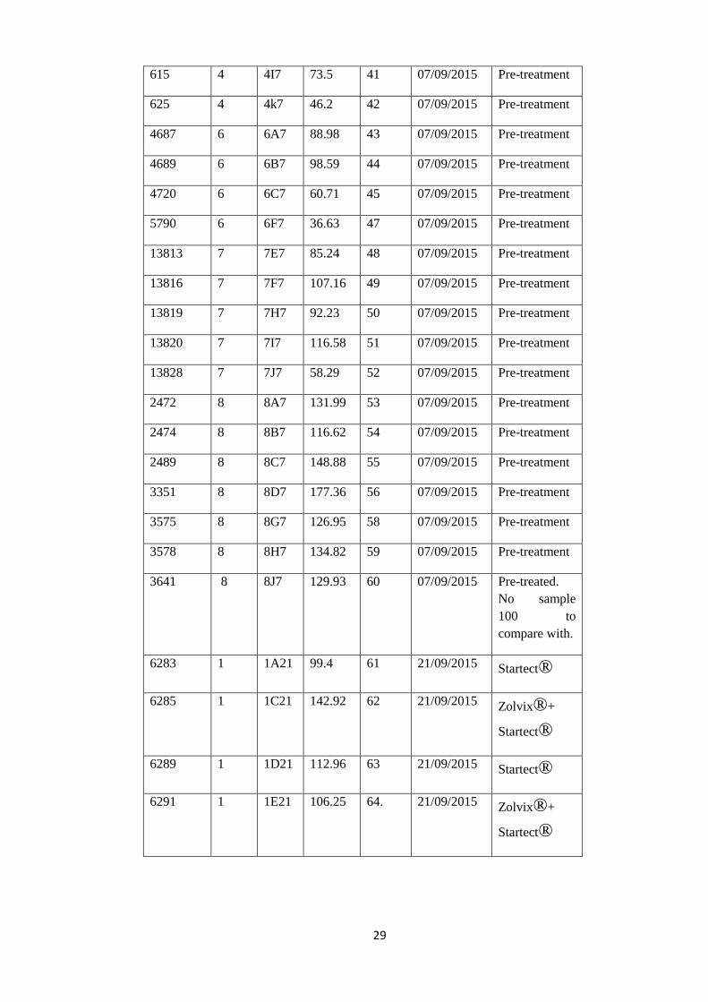
29

615 4 4I7 73.5 41 07/09/2015 Pre-treatment

625 4 4k7 46.2 42 07/09/2015 Pre-treatment

4687 6 6A7 88.98 43 07/09/2015 Pre-treatment

4689 6 6B7 98.59 44 07/09/2015 Pre-treatment

4720 6 6C7 60.71 45 07/09/2015 Pre-treatment

5790 6 6F7 36.63 47 07/09/2015 Pre-treatment

13813 7 7E7 85.24 48 07/09/2015 Pre-treatment

13816 7 7F7 107.16 49 07/09/2015 Pre-treatment

13819 7 7H7 92.23 50 07/09/2015 Pre-treatment

13820 7 7I7 116.58 51 07/09/2015 Pre-treatment

13828 7 7J7 58.29 52 07/09/2015 Pre-treatment

2472 8 8A7 131.99 53 07/09/2015 Pre-treatment

2474 8 8B7 116.62 54 07/09/2015 Pre-treatment

2489 8 8C7 148.88 55 07/09/2015 Pre-treatment

3351 8 8D7 177.36 56 07/09/2015 Pre-treatment

3575 8 8G7 126.95 58 07/09/2015 Pre-treatment

3578 8 8H7 134.82 59 07/09/2015 Pre-treatment

3641 8 8J7 129.93 60 07/09/2015 Pre-treated.

No sample

100 to

compare with.

6283 1 1A21 99.4 61 21/09/2015 Startect®

6285 1 1C21 142.92 62 21/09/2015 Zolvix®+

Startect®

6289 1 1D21 112.96 63 21/09/2015 Startect®

6291 1 1E21 106.25 64. 21/09/2015 Zolvix®+

Startect®

30

6293 1 1F21 71.88 65 21/09/2015 Startect®

6295 1 1G21 81.07 66 21/09/2015 Zolvix®

6350 1 1I21 89.76 67 21/09/2015 Startect®

2279 3 2C21 89.93 68 21/09/2015 Zolvix®

2286 3 2E21 148.53 69 21/09/2015 Zolvix®

2287 3 2F21 91.25 70 21/09/2015 Zolvix®

2294 3 2G21 98.7 71 21/09/2015 Zolvix®

2305 3 2I21 69.23 72 21/09/2015 Zolvix®+

Startect®

2362 3 2J21 100.76 73 21/09/2015 Startect®

586 4 4A21 147.76 74 21/09/2015 Startect®

587 4 4B21 104.95 75 21/09/2015 Zolvix®

588 4 4C21 84.9 76 21/09/2015 Startect®

605 4 4E21 39.75 77 21/09/2015 Zolvix®

609 4 4F21 82.41 78 21/09/2015 Startect®

610 4 4G21 10.74 79 21/09/2015 Zolvix®

613 4 4H21 113.94 80 21/09/2015 Zolvix®+

Startect®

615 4 4I21 82.05 81 21/09/2015 Zolvix®

625 4 4k21 71.42 82 21/09/2015 Zolvix®

4687 6 6A21 81.18 83 21/09/2015 Startect®

31

4689 6 6B21 42.55 84 21/09/2015 Zolvix®

4720 6 6C21 70.68 85 21/09/2015 Zolvix®

5790 6 6F21 55.55 87 21/09/2015 Zolvix®+

Startect®

13813 7 7E21 47.8 88 21/09/2015 Zolvix®

13816 7 7F21 75.29 89 21/09/2015 Zolvix®

13819 7 7H21 125.12 90 21/09/2015 Startect®

13820 7 7I21 98.27 91 21/09/2015 Zolvix®+

Startect®

13828 7 7J21 108.53 92 21/09/2015 Zolvix®+

Startect®

2472 8 8A21 140.66 93 21/09/2015 Zolvix®+

Startect®

2474 8 8B21 116.94 94 21/09/2015 Zolvix®

2489 8 8C21 192.55 95 21/09/2015 Zolvix®+

Startect®

3351 8 8D21 99.62 96 21/09/2015 Startect®

3575 8 8G21 91.84 98 21/09/2015 Startect®

3578 8 8H21 102.51 99 21/09/2015 Zolvic®+

Startect®

4.3 Analysis of Bacterial and Archael community. All the samples were pooled together to form an amplicon library. The bacterial 16SrRNA

gene V4 region amplicons were sequenced by the use of the Illumina barcoded MiSeq

platform. Sequences were separated into different samples based on their respective barcodes

32

(demultiplexed) by the Edinburgh Genomics at the University of Edinburgh. Forward and

reverse reads were paired and reads that were shorter than the expected 400bp PCR product

of the V4 region were filtered out as unsuccessful reads. DNA sequences composing of DNA

from two or more parents (Chimeras) were removed by the use of UCHIME. Denovo OTU

(operational Taxonomic Unit) picking was carried out using QIIME. PyNast (Python Nearest

alignment Space Termination) failures were removed. OTUs that only contain one sequence

(singletons) across the entire database were also remove.

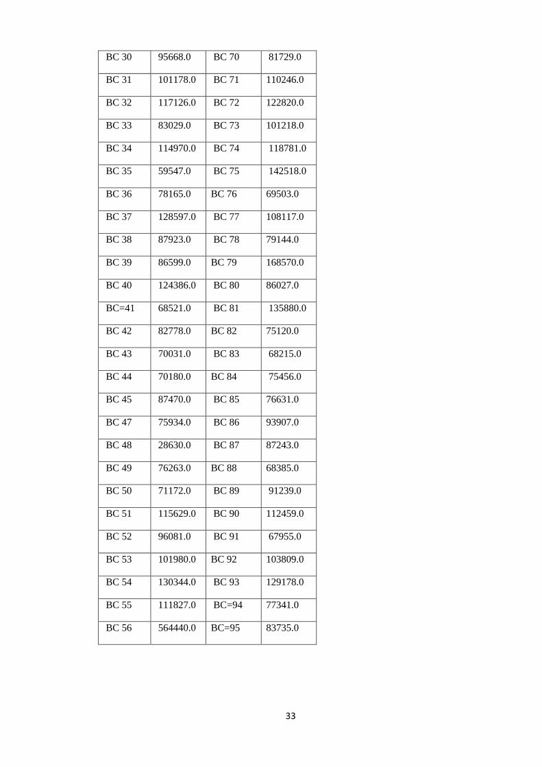
4.4 QIIME Taxonomy Results. Raw sequenced data, obtained from Edinburgh Genomics, for 38 pre-treatment (BC21-

BC60) and the 37 post-treated (BC61-BC99) PCR amplicons, was analysed using the QIIME

pipeline. About 10 million raw data sequences were analysed. However, approximately

36,500 sequences that were less than 240bp were filtered out. Usearch chimeric checking

was performed and 443,328 chimeric sequences were detected and filtered out. Complete

QIIME pipeline analysis was carried out including PyNast (python nearest alignment space

termination) with Greengenes 13_8 been the default database. OTUs were assigned. An

OTU table was made excluding the PyNast failures (11 OTUs). Singletons (227,927 OTUs)

were then removed from the filtered OTU table.

Table 4: OTU Sequence Counts for the Pre-treatment samples (BC21-BC60) and post-

treated samples (BC61-BC99).

Pre-treatment Post-treatment

Barcodes Counts Barcodes Counts

BC 21 79338.0 BC 61 61025.0

BC 22 125786.0 BC 62 110186.0

BC 23 101648.0 BC 63 84886.0

BC 24 89120.0 BC 64 71072.0

BC 25 115771.0 BC 65 74742.0

BC 26 109169.0 BC 66 98736.0

BC 27 89661.0 BC 67 96784.0

BC 28 86304.0 BC 68 80420.0

BC 29 79240.0 BC 69 76100.0

33

BC 30 95668.0 BC 70 81729.0

BC 31 101178.0 BC 71 110246.0

BC 32 117126.0 BC 72 122820.0

BC 33 83029.0 BC 73 101218.0

BC 34 114970.0 BC 74 118781.0

BC 35 59547.0 BC 75 142518.0

BC 36 78165.0 BC 76 69503.0

BC 37 128597.0 BC 77 108117.0

BC 38 87923.0 BC 78 79144.0

BC 39 86599.0 BC 79 168570.0

BC 40 124386.0 BC 80 86027.0

BC=41 68521.0 BC 81 135880.0

BC 42 82778.0 BC 82 75120.0

BC 43 70031.0 BC 83 68215.0

BC 44 70180.0 BC 84 75456.0

BC 45 87470.0 BC 85 76631.0

BC 47 75934.0 BC 86 93907.0

BC 48 28630.0 BC 87 87243.0

BC 49 76263.0 BC 88 68385.0

BC 50 71172.0 BC 89 91239.0

BC 51 115629.0 BC 90 112459.0

BC 52 96081.0 BC 91 67955.0

BC 53 101980.0 BC 92 103809.0

BC 54 130344.0 BC 93 129178.0

BC 55 111827.0 BC=94 77341.0

BC 56 564440.0 BC=95 83735.0

34

BC 58 114452.0 BC 96 81117.0

BC 59 91743.0 BC 98 98168.0

BC 60 114526.0 BC 99 66240.0

As can be seen from table 4, BC 48 had the lowest sequence count of 28,630 while BC 56

had the highest sequence counts of 564,440 sequences from the pre-treatment samples. The

average sequence count for the pre-treated samples was 105,927. For the Post-treated

samples, BC 61 had the lowest sequence count of 61,025 while BC 79 had the highest

sequence count of 168,570. The average sequence count for the post-treated samples was

93,018.

35

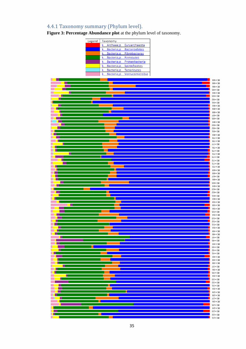
4.4.1 Taxonomy summary (Phylum level). Figure 3: Percentage Abundance plot at the phylum level of taxonomy.

36

At the Phylum level of taxonomy, Bacteroidetes made up 58.76% relative abundance in the

entire microbial population (pre-treatment + post treatment samples). Firmicutes (gram

positive bacteria) made up 28.53% relative abundance of the entire microbial community.

Proteobacteria had a relative abundance of 2.04%. Spirochates were 2.44% in relative

abundance, Tenericutes had a relative abundance of 0.08% while Verrucomicrobia are

2.09% in relative abundance and Euryarchaeota had a relative abundance of 1.12% (Table 5,

Figure 4 and Figure 3).

Table 5: Percentage mean of relative abundance at Phylum level of all samples (Pre-

treatment + Post-treated).

Phylum Mean Standard deviation

Euryarchaeota 1.12% 1.03%

Bacteroidetes 58.76% 6.09%

Fibrobacteres 4.95% 4.19%

Firmicutes 28.53% 5.09%

Proteobacteria 2.04% 2.53%

Spirochaetes 2.44% 2.01%

Tenericutes 0.08% 0.32%

Verrucomicrobia 2.09% 1.62%

37

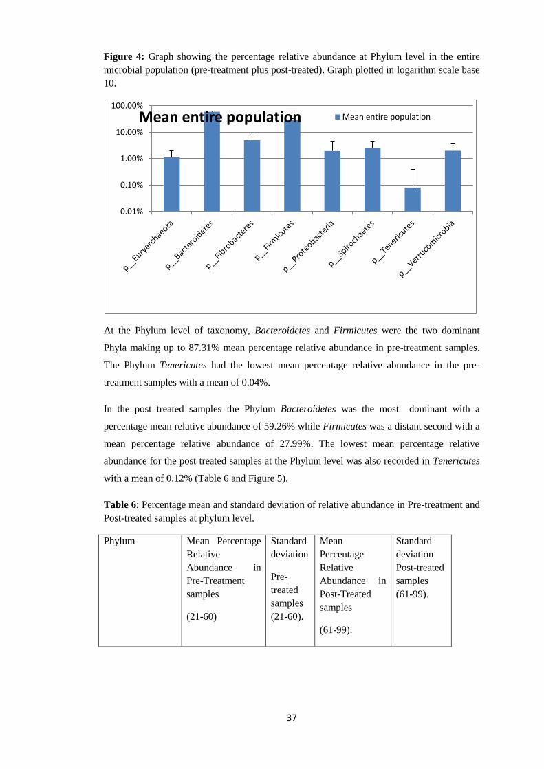
Figure 4: Graph showing the percentage relative abundance at Phylum level in the entire

microbial population (pre-treatment plus post-treated). Graph plotted in logarithm scale base

10.

At the Phylum level of taxonomy, Bacteroidetes and Firmicutes were the two dominant

Phyla making up to 87.31% mean percentage relative abundance in pre-treatment samples.

The Phylum Tenericutes had the lowest mean percentage relative abundance in the pre-

treatment samples with a mean of 0.04%.

In the post treated samples the Phylum Bacteroidetes was the most dominant with a

percentage mean relative abundance of 59.26% while Firmicutes was a distant second with a

mean percentage relative abundance of 27.99%. The lowest mean percentage relative

abundance for the post treated samples at the Phylum level was also recorded in Tenericutes

with a mean of 0.12% (Table 6 and Figure 5).

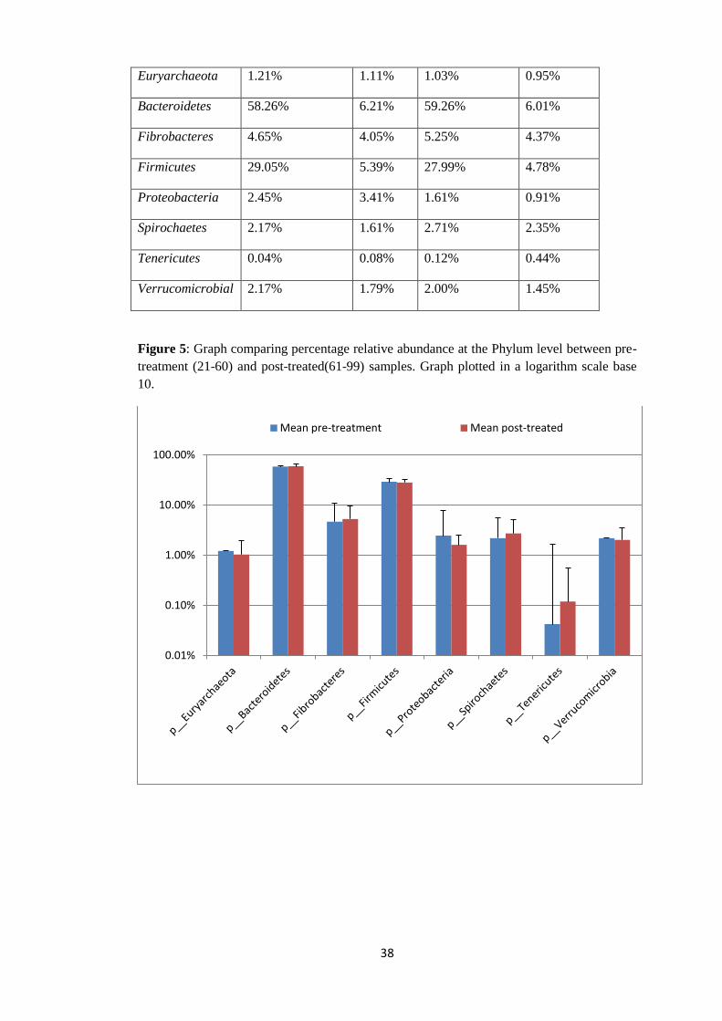
Table 6: Percentage mean and standard deviation of relative abundance in Pre-treatment and

Post-treated samples at phylum level.

Phylum Mean Percentage

Relative

Abundance in

Pre-Treatment

samples

(21-60)

Standard

deviation

Pre-

treated

samples

(21-60).

Mean

Percentage

Relative

Abundance in

Post-Treated

samples

(61-99).

Standard

deviation

Post-treated

samples

(61-99).

0.01%

0.10%

1.00%

10.00%

100.00%

Mean entire population Mean entire population

38

Euryarchaeota 1.21% 1.11% 1.03% 0.95%

Bacteroidetes 58.26% 6.21% 59.26% 6.01%

Fibrobacteres 4.65% 4.05% 5.25% 4.37%

Firmicutes 29.05% 5.39% 27.99% 4.78%

Proteobacteria 2.45% 3.41% 1.61% 0.91%

Spirochaetes 2.17% 1.61% 2.71% 2.35%

Tenericutes 0.04% 0.08% 0.12% 0.44%

Verrucomicrobial 2.17% 1.79% 2.00% 1.45%

Figure 5: Graph comparing percentage relative abundance at the Phylum level between pre-

treatment (21-60) and post-treated(61-99) samples. Graph plotted in a logarithm scale base

10.

0.01%

0.10%

1.00%

10.00%

100.00%

Mean pre-treatment Mean post-treated

39

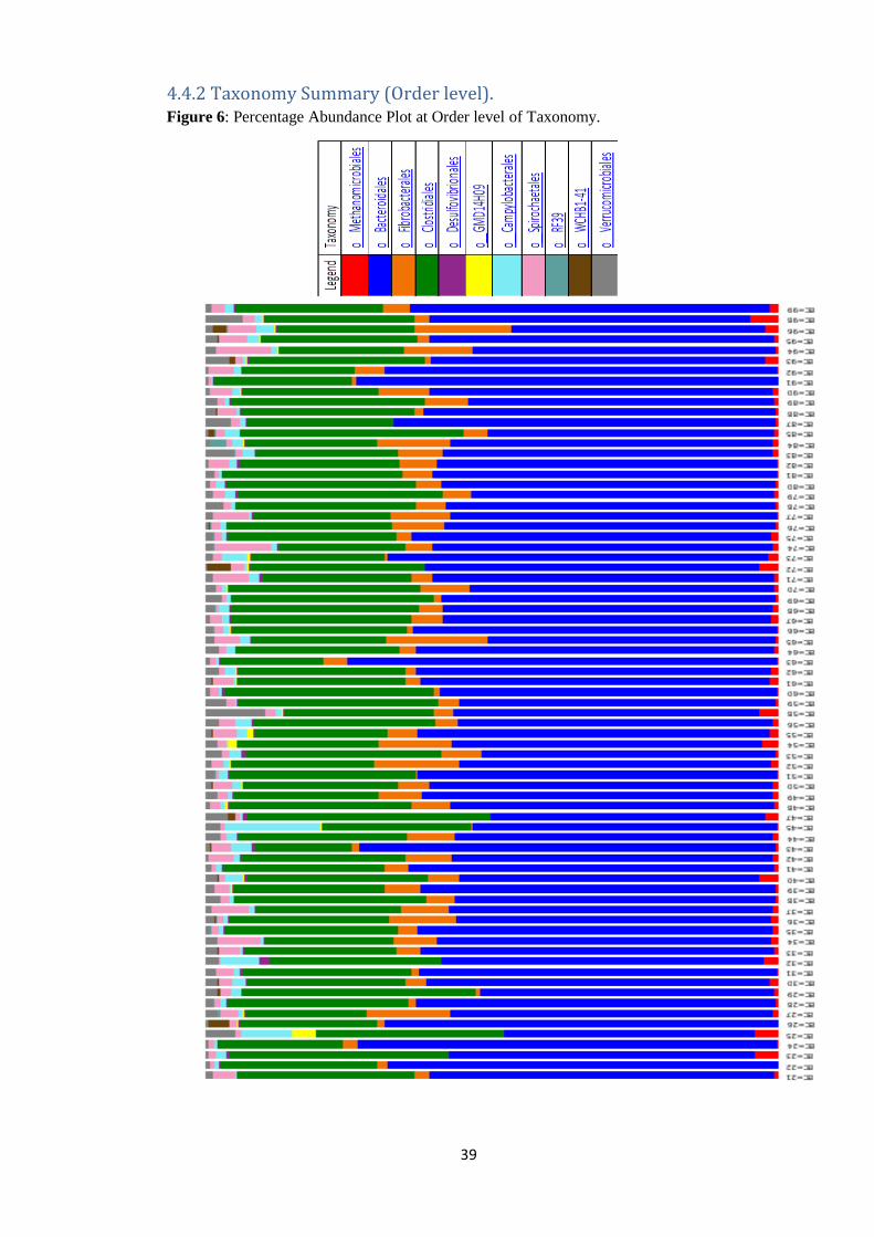
4.4.2 Taxonomy Summary (Order level). Figure 6: Percentage Abundance Plot at Order level of Taxonomy.

40

At the Order level of taxonomy, Bacteroidales and Clostridales made up to 87.30% of the

mean percentage relative abundance of the entire population (pre-treatment + post

treatment). The lowest percentage mean relative abundance at the order level of taxonomy

was seen in the uncultured Order RF39 from the Class Mollicutes which stood at 0.10%

(Table 7, Figure 7 and Figure 6).

Table 7: Combine percentage mean of relative abundance at order level of all samples (Pre-

treatment + Post-treated).

Order Mean percentage

relative

abundance (Pre-

treatment + Post

treated.

Standard deviation entire

population (Pre-treatment +

Post-treatment)

Methanomicrobiales 1.10% 1.03%

Bacteroidales 58.80% 6.09%

Fibrobacterales 4.90% 4.19%

Clostridiales 28.50% 5.09%

Desulfovibrionales 0.30% 0.22%

GMD14H09 0.20% 0.52%

Campylobacterales 1.60% 2.25%

Spirochaetales 2.40% 2.01%

Uncultured,Order

RF39, Mollicutes

0.10% 0.32%

Uncultured,Genus

WCHB1-41,Class

Verruco-5

0.20% 0.71%

Verrucomicrobiales 1.90% 1.56%

41

Figure 7: Graph showing the percentage relative abundance at Order level in the entire

microbial population (pre-treatment + post-treated). Graph plotted in logarithm scale base

10.

Bacteroidales and Clostridales were the dominant Orders in the pre-treatment samples with

relative abundance of 58.26% and 29.05% respectively. The least dominant order in the pre-

treatment sample was recorded in the uncultured Order RF39 from the Class Mollicutes with

a mean percentage relative abundance of 0.04% (Table 8, figure 8).

For the post-treated samples (61-99) at the Order level of taxonomy, Bacteroidales was

again dominant with a mean percentage relative abundance of 59.26% while the lowest

mean was seen in the uncultured Order Delta GMD14H09 ( Table 8 and Figure 8).

Table 8: Percentage mean and standard deviation of relative abundance in Pre-treatment and

Post-treated samples at Order level of taxonomy.

0.01%

0.10%

1.00%

10.00%

100.00%

Mean at order level Entire population Mean at order level Entire population

Order Mean Pre-

treatment

samples

(21-60).

Standard

deviation

Pre-

treatment

samples

Mean post-

treated

samples

(61-99).

Standard deviation

Post-Treated samples

(61-99).

42

(21-60).

Methanomicrobiales 1.21% 1.11% 1.03% 0.95%

Bacteroidales 58.26% 6.21% 59.26% 6.01%

Fibrobacterales 4.65% 4.05% 5.25% 4.37%

Clostridiales 29.05% 5.39% 27.99% 4.78%

Desulfovibrionales 0.31% 0.29% 0.23% 0.11%

Uncultured

Deltaproteobacterium

GMD14H09

0.24% 0.72% 0.08% 0.11%

Campylobacterales 1.89% 3.04% 1.31% 0.84%

Spirochaetales 2.17% 1.61% 2.71% 2.35%

Uncultured,Genus

RF39,Class

Mollicutes

0.04% 0.08% 0.12% 0.44%

Uncultured,Genus

WCHB1-41,Class

Verruco-5

0.20% 0.61% 0.26% 0.81%

Verrucomicrobiales 1.97% 1.75% 1.74% 1.36%

43

Figure 8: Graph of mean relative abundance in pre-treatment samples (21-60) and post

treated samples (61-99) at Order level of Taxonomy.

44

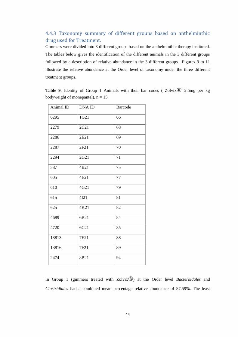
4.4.3 Taxonomy summary of different groups based on anthelminthic

drug used for Treatment. Gimmers were divided into 3 different groups based on the anthelminthic therapy instituted.

The tables below gives the identification of the different animals in the 3 different groups

followed by a description of relative abundance in the 3 different groups. Figures 9 to 11

illustrate the relative abundance at the Order level of taxonomy under the three different

treatment groups.

Table 9: Identity of Group 1 Animals with their bar codes ( Zolvix® 2.5mg per kg

bodyweight of monepantel). n = 15.

Animal ID DNA ID Barcode

6295 1G21 66

2279 2C21 68

2286 2E21 69

2287 2F21 70

2294 2G21 71

587 4B21 75

605 4E21 77

610 4G21 79

615 4I21 81

625 4K21 82

4689 6B21 84

4720 6C21 85

13813 7E21 88

13816 7F21 89

2474 8B21 94

In Group 1 (gimmers treated with Zolvix®) at the Order level Bacteroidales and

Clostridiales had a combined mean percentage relative abundance of 87.59%. The least

45

dominant in mean percentage relative abundance was the uncultured Order GMD14H09 from

the Class Deltaproteobacteria with a mean percentage relative abundance of 0.07% ( Table

10, Figure 9).

Table 10. Percentage mean and standard deviation of relative abundance in group 1 (treated

with Zolvix®) (2.5mg per kg bodyweight of Monepantel). n = 15

Order Mean Standard deviation.






Uncultured Order

GMD14H09,Class

Deltaproteobacteria

0.07% 0.09%



Uncultured Order RF39

Class Mollicutes

0.25% 0.68%

Uncultured Order WCHB1-

41 Class Verruco-5

0.11% 0.33%


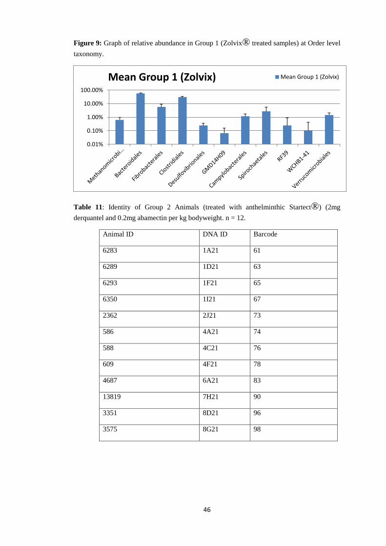
46

Figure 9: Graph of relative abundance in Group 1 (Zolvix® treated samples) at Order level

taxonomy.

Table 11: Identity of Group 2 Animals (treated with anthelminthic Startect®) (2mg

derquantel and 0.2mg abamectin per kg bodyweight. n = 12.

Animal ID DNA ID Barcode

6283 1A21 61

6289 1D21 63

6293 1F21 65

6350 1I21 67

2362 2J21 73

586 4A21 74

588 4C21 76

609 4F21 78

4687 6A21 83

13819 7H21 90

3351 8D21 96

3575 8G21 98

0.01%

0.10%

1.00%

10.00%

100.00%

Mean Group 1 (Zolvix) Mean Group 1 (Zolvix)

47

In Group 2 (animals treated with Startect®) the Order Bacteroidales had a mean percentage

relative abundance of 58.56% while Clostridiales had a mean percentage relative abundance

of 25.53%. Uncultured Order RF39 from the Class Mollicutes was the least dominant with a

mean percentage relative abundance of 0.05% in group 2 samples (Table 12, Figure 10).

Table 12: Percentage mean and standard deviation of relative abundance in group 2

:Startect® (2mg derquantel and 0.2mg abamectin per kg bodyweight). n = 12

Order Mean Standard deviation






Uncultured,Order

GMD14H09,Class

Deltaproteobacteria

0.12% 0.14%



Uncultured Order RF39,

Mollicutes

0.05% 0.09%

Uncultured Order WCHB1-41

Class Verruco-5

0.22% 0.69%


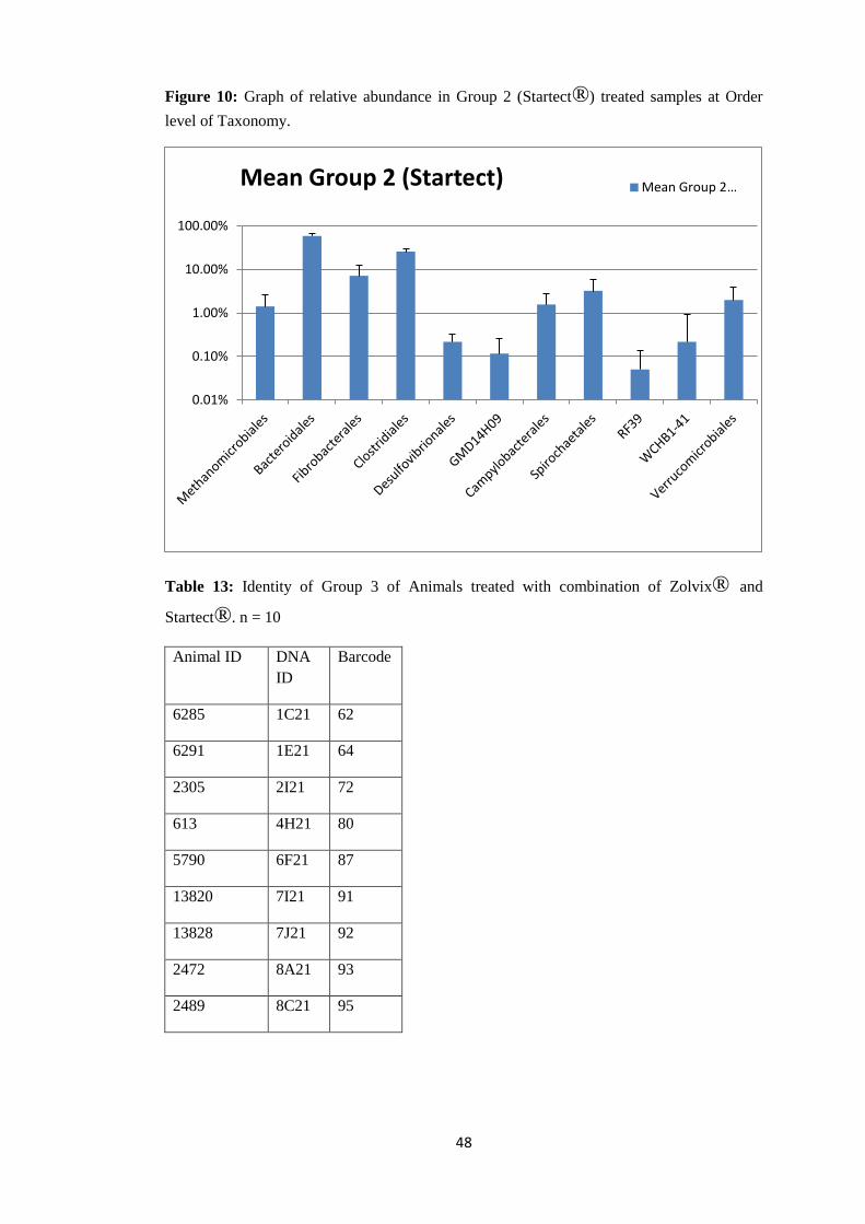
48

Figure 10: Graph of relative abundance in Group 2 (Startect®) treated samples at Order

level of Taxonomy.

Table 13: Identity of Group 3 of Animals treated with combination of Zolvix® and

Startect®. n = 10

Animal ID DNA

ID

Barcode

6285 1C21 62

6291 1E21 64

2305 2I21 72

613 4H21 80

5790 6F21 87

13820 7I21 91

13828 7J21 92

2472 8A21 93

2489 8C21 95

0.01%

0.10%

1.00%

10.00%

100.00%

Mean Group 2 (Startect) Mean Group 2 …

49

3578 8H21 99

The highest average relative abundance in Group 3 (gimmers treated with a combination of

Zolvix® and Startect®) was seen in the order Bacteroidales at 63.13%. Clostridiales was a

distant second with a mean of 27.43%. The uncultured Order RF39 from the Class

Mollicutes was also the least in relative abundance in this group with a mean of 0.01%

(Table 14, Figure 11).

Table 14: Percentage mean and standard deviation of relative abundance in group 3.

Combination of Zolvix® (2.5mg per kg bodyweight of monepantel) and Startect® (2mg

derquantel and 0.2mg abamectin per kg bodyweight). n = 10.

Order level of Taxonomy Mean Standard deviation.






Uncultured,Order

GMD14H09,Class

Deltaproteobacteria

0.06% 0.11%



Uncultured Order RF39,

Class Mollicutes

0.01% 0.03%

UnculturedOrder WCHB1-

41, Class Verruco-5.

0.55% 1.31%


50

Figure 11: Graph of relative abundance in Zolvix® + Startect® treated samples to the

Taxonomic level of Order.

The mean percentage relative abundance in each of the post treated groups was compared.

Bacteroidales had the highest mean percentage relative abundance of 63.13% in the group 3,

it stood at 58.56% in group 2 samples and 57. 25% in group 1 samples. Clostridiales

recorded the highest mean percentage relative abundance of 30.34% in group 1, closely

followed by a mean percentage relative abundance of 27.43% in group 3 samples.

Uncultured Order RF39 from the Class Mollicutes had a mean percentage relative abundance

of 0.25% in group 1, 0.05% in group 2 and 0.01% in group 3 (Table 15, Figure 12).

Table 15: Percentage mean of relative abundance in group 1, group 2, and group 3

Order Mean Group 1

(Zolvix®)

Mean

Group 2

(Startect

®)

Mean Group 3

(Zolvix® +

Startect®)

Methanomicrobiales 0.63% 1.42% 1.15%

Bacteroidales 57.25% 58.56% 63.13%

Fibrobacterales 5.73% 7.12% 2.28%

0.01%

0.10%

1.00%

10.00%

100.00%

Mean Group 3 (Zolvix + Startect) Mean Group 3(Zolvix + …

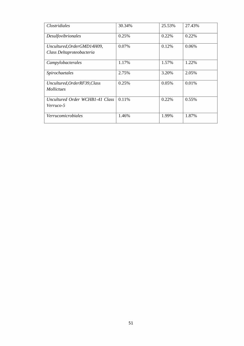
51

Clostridiales 30.34% 25.53% 27.43%

Desulfovibrionales 0.25% 0.22% 0.22%

Uncultured,OrderGMD14H09,

Class Deltaproteobacteria

0.07% 0.12% 0.06%

Campylobacterales 1.17% 1.57% 1.22%

Spirochaetales 2.75% 3.20% 2.05%

Uncultured,OrderRF39,Class

Mollictues

0.25% 0.05% 0.01%

Uncultured Order WCHB1-41 Class

Verruco-5

0.11% 0.22% 0.55%

Verrucomicrobiales 1.46% 1.99% 1.87%

52

Figure 12: Graph of mean relative abundance in Group 1, Group 2 and Group 3 Order level

of taxonomy.

53

The mean percentage relative abundance in the pre – treatment samples was compared with

the mean percentage relative abundance in different groups of the post – treated samples

(group 1, group 2 and group 3). The Order Bacteroidales had a mean percentage relative

abundance of 58.26% in the pre – treated samples, 63.13% in group 3, 58.56% in group 2,

57.25% in group 1. The order Clostridiales had a mean percentage relative abundance of

29.05% in the pre-treatment samples and a mean of 30.34% in group 1. Clostridiales also

recorded a mean of 25.53% in group 2, and 27.43% in group 3. Campylobacterales had a

mean percentage relative abundance of 1.89% in the pre-treatment samples. In group 1

Campylobacterales had a mean of 1.17%, a mean of 1.57% in group 2 and a mean of 1.22%

in the group 3 samples (Table 16, Figure 13).

Table 16: Percentage mean relative abundance in Pre-treated, Group 1, Group 2, Group 3 at

Order level of Taxonomy.

Order level of

Taxonomy

Mean Pre-

treatment

(21-60)

Mean Group 1

(Zolvix®)

Mean Group 2

(Startect®)

Mean

Group 3

(Zolvix® +

Startect®)


Bacteroidales 58.26% 57.25% 58.56% 63.13%


Clostridiales 29.05% 30.34% 25.53% 27.43%


Uncultured Order

GMD14H09, Class

Deltaproteobacteria

0.24% 0.07% 0.12% 0.06%


Spirochaetales 2.17% 2.75% 3.20% 2.05%

Uncultured Order,

RF39, Class

Mollicutes

0.04% 0.25% 0.05% 0.01%

Uncultured Order

WCHB1-41, Class

Verruco-5

0.20% 0.11% 0.22% 0.55%

54


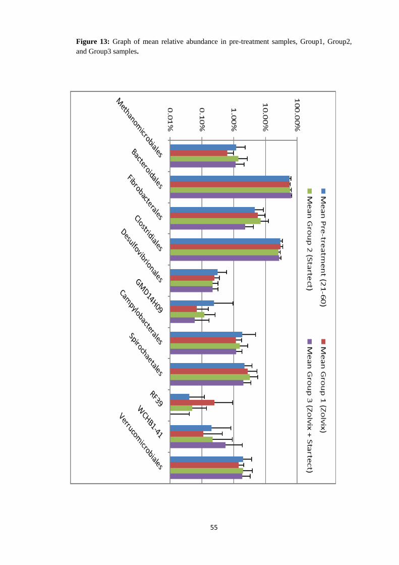
55

Figure 13: Graph of mean relative abundance in pre-treatment samples, Group1, Group2,

and Group3 samples.

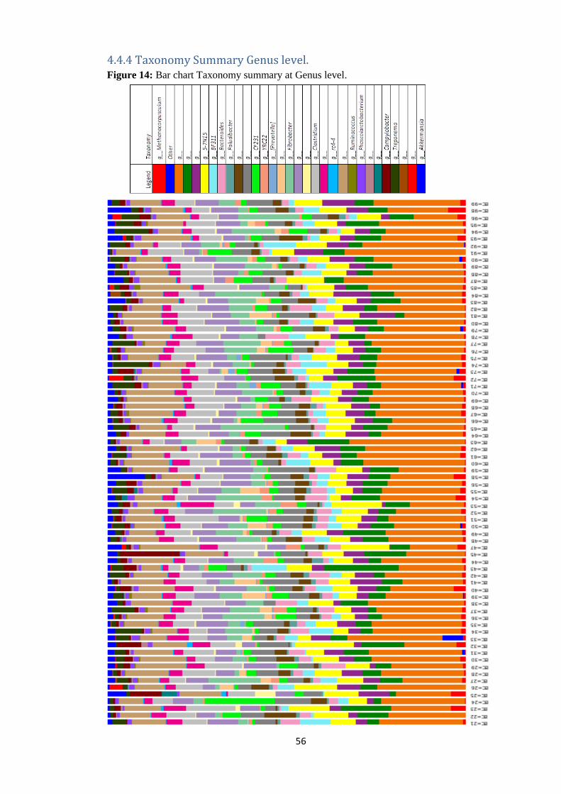
56

4.4.4 Taxonomy Summary Genus level. Figure 14: Bar chart Taxonomy summary at Genus level.

57

At the Genus level of Taxonomy, an uncultured genus from the Order Bacteroidales was the

most dominant Genus with a percentage mean relative abundance of 22.27% and a standard

deviation of 4.35% in the entire population. An uncultured Genus from the Family

Ruminococcaceae was a distant second in dominance with a mean of 9.73% closely followed

by the Genus Clostridium which had a mean of 7.19%. The lowest mean percentage relative

abundance at the Genus level of 0.08% was recorded in an uncultured Genus from the

uncultured Order RF39 from the Class Mollicutes (Table 17, Figure 15 and Figure 14).

Table 17: Percentage mean relative abundance at Genus level in all samples.

Genus Mean Standard deviation

Methanocorpusculum 1.12% 1.03%

Uncultured Genus, Order

Bacterooidales

0.15% 0.69%


Bacteroidales

22.27% 4.35%


Bacteroidales

5.97% 3.05%

Uncultured Genus, Family

Bacteroidaceae

4.43% 2.07%

Uncultured Genus 5-7N15,

Family Bacteroidaceae

6.58% 2.42%

Uncultured Genus BF311


2.71% 2.24%

Bacteroides 2.88% 1.61%

Paludibacter 0.76% 0.56%


Bacterooidales

2.46% 1.61%


Rikenellaceae

5.57% 1.88%

Uncultured Genus CF231,

Family Paraprevotellaceae

2.70% 2.61%

Uncultured Genus YRC22


1.05% 1.04%

58

[Prevotella] 0.15% 0.36%


Bacterooidales

1.06% 1.76%

Fibrobacter 4.95% 4.19%


Clostridiales

6.32% 1.93%


Christensenellaceae

0.46% 0.69%

Clostridium 7.19% 2.11%


Lachnospiraceae

3.17% 1.48%

Uncultured Genus rc4-4,

Family Peptococcaceae

0.31% 0.25%


Ruminococcaceae

9.73% 2.50%

Ruminococcus 0.22% 0.29%

Phascolarctobacterium 1.13% 0.36%


Desulfovibrionaceae

0.27% 0.22%

Uncultured Genus, Class

Deltaproteobacteria

0.16% 0.52%

Campylobacter 1.60% 2.25%

Treponema 2.44% 2.01%


Mollicutes

0.08% 0.32%


Verruco-5

0.23% 0.71%

Akkermansia 1.86% 1.56%

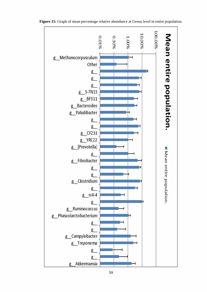
59

Figure 15: Graph of mean percentage relative abundance at Genus level in entire population.

60

In the pre-treatment samples, an uncultured Genus from the Order Bacteroidales was the

most dominant with a mean percentage relative abundance of 20.85% and a standard

deviation of 3.78%. An uncultured Genus from the Family Ruminococcaceae had a mean of

9.60% with a standard deviation of 2.32% making it second in dominance. The uncultured

Genus from the Uncultured Order RF39 from the Class Mollicutes was the least dominant

with a mean of 0.04% (Table 18, Figure 16).

Table 18: Mean percentage relative abundance at Genus level in Pre-treatment samples.

Taxonomy Mean Pre-treatment

Genus level.

Standard deviation

Pre-treatment



Bacterooidales

0.20% 0.94%


Bacteroidales

20.85% 3.78%


Bacteroidales

6.35% 3.71%


Bacteroidaceae

3.94% 1.89%



7.00% 2.99%



2.73% 2.38%




Bacterooidales

2.42% 1.75%


Rikenellaceae

5.65% 2.08%



2.65% 3.20%

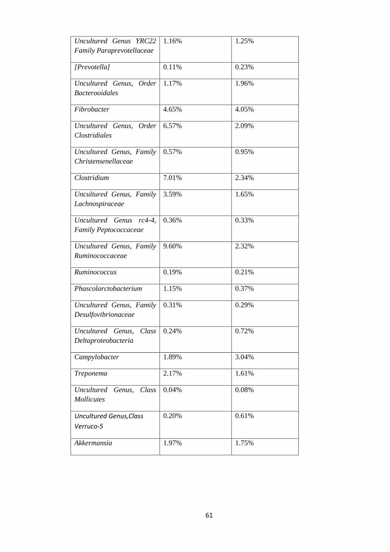
61



1.16% 1.25%



Bacterooidales

1.17% 1.96%



Clostridiales

6.57% 2.09%


Christensenellaceae

0.57% 0.95%



Lachnospiraceae

3.59% 1.65%



0.36% 0.33%


Ruminococcaceae

9.60% 2.32%




Desulfovibrionaceae

0.31% 0.29%


Deltaproteobacteria

0.24% 0.72%




Mollicutes

0.04% 0.08%

Uncultured Genus,Class

Verruco-5

0.20% 0.61%


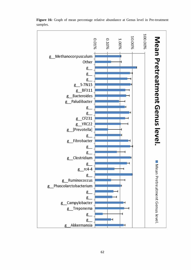
62

Figure 16: Graph of mean percentage relative abundance at Genus level in Pre-treatment

samples.

63

The Genus that was dominant in the post treated sample was again the uncultured Genus

from the Order Bacteroidales with a mean percentage relative abundance of 23.73% and a

standard deviation of 4.46%. An uncultured Genus from the Family Ruminococcaceae with

a mean of 9.86% and a standard deviation of 2.70% was second in dominance. The least with

mean relative abundance of 0.08% was the uncultured Genus from the uncultured Order

GMD14H09 from the class Deltaproteobacteria (Table 19, Figure 17).

Table 19: Mean percentage relative abundance at Genus level in Post treated samples.

Taxonomy Mean Post-treatment Genus

level

Standard deviation Post-

treated Genus level.



Bacterooidales

0.09% 0.26%


Bacteroidales

23.73% 4.46%


Bacteroidales

5.59% 2.17%


Bacteroidaceae

4.93% 2.15%



6.15% 1.58%



2.69% 2.12%




Bacterooidales

2.50% 1.48%


Rikenellaceae

5.48% 1.66%



2.74% 1.86%

Uncultured Genus YRC22 0.95% 0.79%

64




Bacterooidales

0.95% 1.56%



Clostridiales

6.06% 1.75%


Christensenellaceae

0.35% 0.17%



Lachnospiraceae

2.74% 1.14%



0.26% 0.12%


Ruminococcaceae

9.86% 2.70%




Desulfovibrionaceae

0.23% 0.11%

Uncultured Genus

GMD14H09, Class

Deltaproteobacteria

0.08% 0.11%




Mollicutes

0.12% 0.44%


Verruco-5

0.26% 0.81%


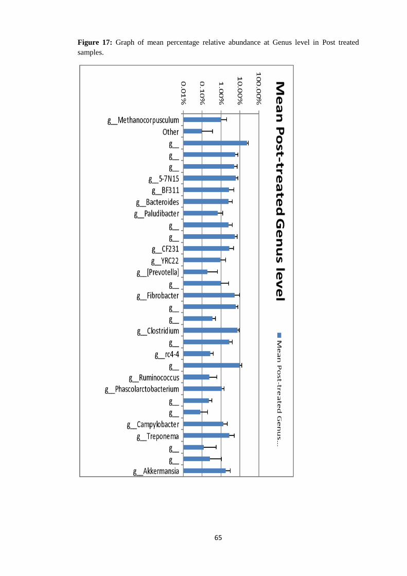
65

Figure 17: Graph of mean percentage relative abundance at Genus level in Post treated

samples.

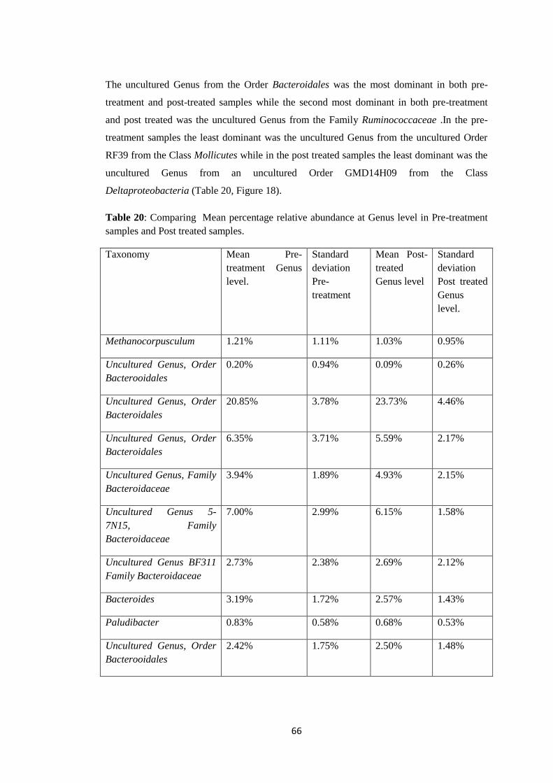
66

The uncultured Genus from the Order Bacteroidales was the most dominant in both pre-

treatment and post-treated samples while the second most dominant in both pre-treatment

and post treated was the uncultured Genus from the Family Ruminococcaceae .In the pre-

treatment samples the least dominant was the uncultured Genus from the uncultured Order

RF39 from the Class Mollicutes while in the post treated samples the least dominant was the

uncultured Genus from an uncultured Order GMD14H09 from the Class

Deltaproteobacteria (Table 20, Figure 18).

Table 20: Comparing Mean percentage relative abundance at Genus level in Pre-treatment

samples and Post treated samples.

Taxonomy Mean Pre-

treatment Genus

level.

Standard

deviation

Pre-

treatment

Mean Post-

treated

Genus level

Standard

deviation

Post treated

Genus

level.

Methanocorpusculum 1.21% 1.11% 1.03% 0.95%


Bacterooidales

0.20% 0.94% 0.09% 0.26%


Bacteroidales

20.85% 3.78% 23.73% 4.46%


Bacteroidales

6.35% 3.71% 5.59% 2.17%


Bacteroidaceae

3.94% 1.89% 4.93% 2.15%

Uncultured Genus 5-

7N15, Family

Bacteroidaceae

7.00% 2.99% 6.15% 1.58%



2.73% 2.38% 2.69% 2.12%

Bacteroides 3.19% 1.72% 2.57% 1.43%

Paludibacter 0.83% 0.58% 0.68% 0.53%


Bacterooidales

2.42% 1.75% 2.50% 1.48%

67


Rikenellaceae

5.65% 2.08% 5.48% 1.66%


Family

Paraprevotellaceae

2.65% 3.20% 2.74% 1.86%


Family

Paraprevotellaceae

1.16% 1.25% 0.95% 0.79%

[Prevotella] 0.11% 0.23% 0.19% 0.46%


Bacterooidales

1.17% 1.96% 0.95% 1.56%

Fibrobacter 4.65% 4.05% 5.25% 4.37%


Clostridiales

6.57% 2.09% 6.06% 1.75%


Christensenellaceae

0.57% 0.95% 0.35% 0.17%

Clostridium 7.01% 2.34% 7.37% 1.85%


Lachnospiraceae

3.59% 1.65% 2.74% 1.14%



0.36% 0.33% 0.26% 0.12%


Ruminococcaceae

9.60% 2.32% 9.86% 2.70%

Ruminococcus 0.19% 0.21% 0.24% 0.35%

Phascolarctobacterium 1.15% 0.37% 1.11% 0.36%


Desulfovibrionaceae

0.31% 0.29% 0.23% 0.11%


Deltaproteobacteria

0.24% 0.72% 0.08% 0.11%

Campylobacter 1.89% 3.04% 1.31% 0.84%

Treponema 2.17% 1.61% 2.71% 2.35%

Uncultured Genus, Class 0.04% 0.08% 0.12% 0.44%

68

Mollicutes


Verruco-5

0.20% 0.61% 0.26% 0.81%

Akkermansia 1.97% 1.75% 1.74% 1.36%

69

Figure 18: Graph comparing the mean percentage relative abundance at Genus level pre-

treatment and post treated samples.

70

In group 1 (Zolvix®), the uncultured Genus from the Order Bacteroidales was the most

dominant with a mean percentage relative abundance of 22.86% and a standard deviation of

2.96%. The uncultured Genus from the Family Ruminococcaceae was a distant second with

a mean of 10.34% closely followed by the Genus Clostridium with a mean of 8.09%. The

lowest mean percentage relative abundance of 0.07% was observed in the uncultured Genus

from the uncultured Order GMD14H09 from the Class Deltaproteobacteria (Table 21,

Figure 19).

Table 21: Mean percentage relative abundance at Genus level in Group 1 (Zolvix®).

Taxonomy Mean Genus level

Group 1

Standard deviation

Genus level Group 1



Bacterooidales

0.10% 0.27%


Bacteroidales

22.86% 2.96%


Bacteroidales

4.53% 1.52%


Bacteroidaceae

5.13% 2.25%



5.99% 1.56%

Uncultured Genus BF311 Family

Bacteroidaceae

2.23% 2.02%




Bacterooidales

1.97% 0.95%

Uncultured Genus, Family 5.61% 2.08%

71

Rikenellaceae

Uncultured Genus CF231, Family

Paraprevotellaceae

2.94% 1.80%

Uncultured Genus YRC22 Family

Paraprevotellaceae

0.97% 0.83%



Bacterooidales

1.08% 1.74%



Clostridiales

6.56% 1.81%


Christensenellaceae

0.38% 0.18%



Lachnospiraceae

3.18% 0.67%

Uncultured Genus rc4-4, Family

Peptococcaceae

0.29% 0.13%


Ruminococcaceae

10.34% 3.23%




Desulfovibrionaceae

0.25% 0.11%


Deltaproteobacteria

0.07% 0.09%




Mollicutes

0.25% 0.68%

72

UnculturedGenus,Class,Verruco

-5

0.11% 0.33%


73

Figure 19: Graph showing percentage relative abundance at Genus in Group 1 (Zolvix®).

s

74

In the group 2 (Startect®), the uncultured Genus from the Order Bacteroidales was

dominant with a mean percentage relative abundance of 22.87%. A distant second was an

uncultured Genus from the Family Ruminococcaceae with a mean percentage relative

abundance of 9.03%. Fibrobacter had a mean percentage relative abundance of 7.12%

which was closely followed by Clostridium that recorded a mean of 6.21%. The lowest mean

percentage relative abundance was recorded in the uncultured Genus from the uncultured

Order RF39 from the Class Mollicutes (Table 22, figure20).

Table 22: Mean percentage relative abundance at Genus level in Group 2 (Startect®).

Genus Mean Genus level

Group 2

Standard deviation Genus level

Group 2



Bacterooidales

0.14% 0.33%


Bacteroidales

22.87% 5.54%


Bacteroidales

6.19% 2.41%


Bacteroidaceae

4.38% 1.51%



5.98% 1.37%



3.24% 1.81%




Bacterooidales

2.64% 1.42%


Rikenellaceae

5.01% 1.37%



2.46% 1.90%

75



0.67% 0.53%



Bacterooidales

1.28% 1.81%



Clostridiales

5.80% 1.59%


Christensenellaceae

0.33% 0.16%



Lachnospiraceae

2.47% 1.22%



0.28% 0.12%


Ruminococcaceae

9.03% 1.82%




Desulfovibrionaceae

0.22% 0.10%


Deltaproteobacteria

0.12% 0.14%




Mollicutes

0.05% 0.09%

UnculturedGenus,ClassVer

ruco-5

0.22% 0.69%


76

Figure 20: Graph showing percentage relative abundance at Genus level in Group 2

(Startect®).

77

In Group 3 (Zolvix® + Startect®), the uncultured Genus from the Order Bacteroidales

recorded the highest mean percentage relative abundance 26.07%. An Uncultured Genus

from the Family Ruminococcaceae was second with a mean of 10.14%. The lowest mean

was observed in an uncultured Genus from the un cultured Order RF39 from the Class

Mollicutes (Table 23, Figure 21).

Table 23: Mean percentage relative abundance at Genus level in Group 3

Taxonomy Mean Genus level

Group 3

Standard deviation Genus level Group

3



Bacterooidales

0.03% 0.09%


Bacteroidales

26.07% 4.49%


Bacteroidales

6.46% 2.23%

Uncultured Genus,


5.28% 2.69%

Uncultured Genus 5-

7N15, Family

Bacteroidaceae

6.61% 1.87%



2.71% 2.62%




Bacterooidales

3.13% 1.99%

Uncultured Genus,

Family Rikenellaceae

5.85% 1.26%

Uncultured Genus

CF231, Family

Paraprevotellaceae

2.79% 2.04%

78


Family

Paraprevotellaceae

1.25% 0.92%



Bacterooidales

0.36% 0.63%



Clostridiales

5.62% 1.83%

Uncultured Genus,

Family

Christensenellaceae

0.33% 0.17%


Uncultured Genus,

Family Lachnospiraceae

2.42% 1.45%



0.21% 0.10%

Uncultured Genus,

Family

Ruminococcaceae

10.14% 2.73%



Uncultured Genus,

Family

Desulfovibrionaceae

0.22% 0.10%


Deltaproteobacteria

0.06% 0.11%




Mollicutes

0.01% 0.03%

Uncultured Genus,Class 0.55% 1.31%

79

Verruco-5


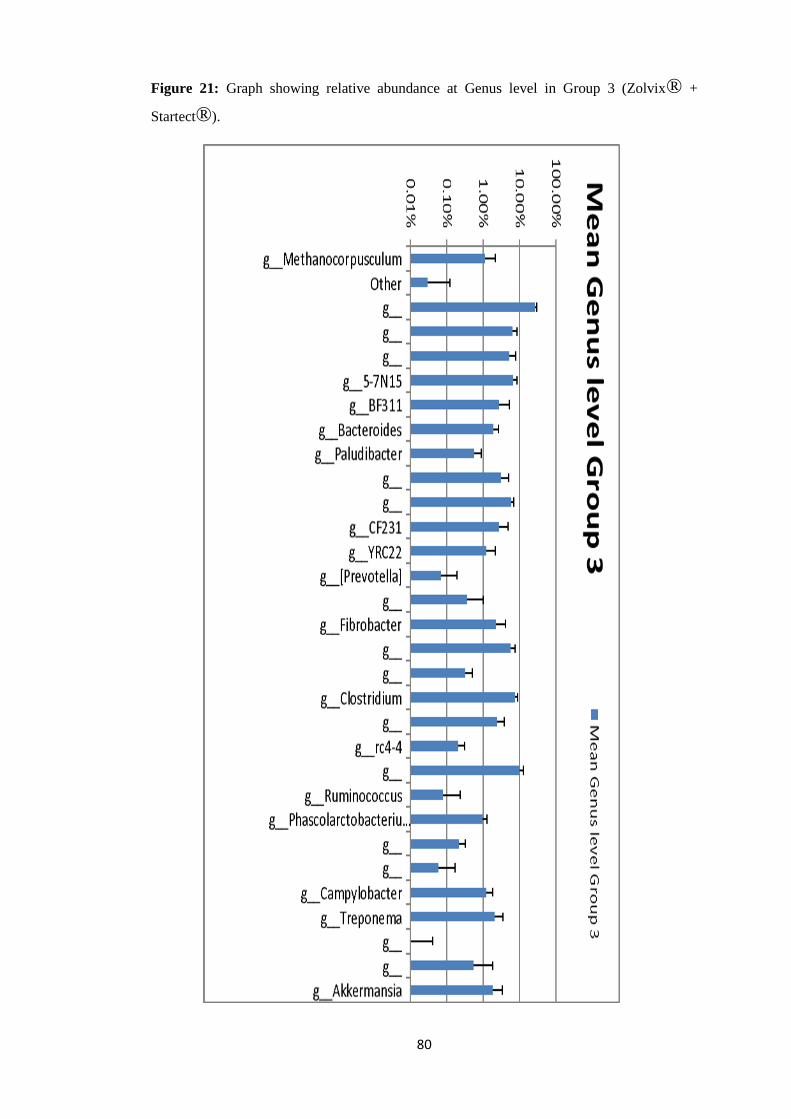
80

Figure 21: Graph showing relative abundance at Genus level in Group 3 (Zolvix® +

Startect®).

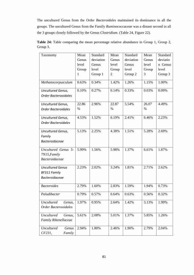
81

The uncultured Genus from the Order Bacteroidales maintained its dominance in all the

groups. The uncultured Genus from the Family Ruminococcaceae was a distant second in all

the 3 groups closely followed by the Genus Clostridium. (Table 24, Figure 22).

Table 24: Table comparing the mean percentage relative abundance in Group 1, Group 2,

Group 3.

Taxonomy Mean

Genus

level

Group

1

Standard

deviation

Genus

level

Group 1

Mean

Genus

level

Group

2

Standard

deviation

Genus

level

Group 2

Mean

Genus

level

Group

3

Standard

deviatio

n Genus

level

Group 3

Methanocorpusculum 0.63% 0.34% 1.42% 1.26% 1.15% 1.00%

Uncultured Genus,

Order Bacterooidales

0.10% 0.27% 0.14% 0.33% 0.03% 0.09%

Uncultured Genus,

Order Bacteroidales

22.86

%

2.96% 22.87

%

5.54% 26.07

%

4.49%

Uncultured Genus,

Order Bacteroidales

4.53% 1.52% 6.19% 2.41% 6.46% 2.23%

Uncultured Genus,

Family

Bacteroidaceae

5.13% 2.25% 4.38% 1.51% 5.28% 2.69%

Uncultured Genus 5-

7N15,Family

Bacteroidaceae

5.99% 1.56% 5.98% 1.37% 6.61% 1.87%

Uncultured Genus

BF311 Family

Bacteroidaceae

2.23% 2.02% 3.24% 1.81% 2.71% 2.62%

Bacteroides 2.79% 1.60% 2.83% 1.59% 1.94% 0.73%

Paludibacter 0.79% 0.57% 0.64% 0.63% 0.56% 0.32%

Uncultured Genus,


1.97% 0.95% 2.64% 1.42% 3.13% 1.99%

Uncultured Genus,


5.61% 2.08% 5.01% 1.37% 5.85% 1.26%

Uncultured Genus

CF231, Family

2.94% 1.80% 2.46% 1.90% 2.79% 2.04%

82

Paraprevotellaceae

Uncultured Genus

YRC22 Family

Paraprevotellaceae

0.97% 0.83% 0.67% 0.53% 1.25% 0.92%

[Prevotella] 0.25% 0.53% 0.21% 0.54% 0.07% 0.13%

Uncultured Genus,


1.08% 1.74% 1.28% 1.81% 0.36% 0.63%

Fibrobacter 5.73% 3.79% 7.12% 5.38% 2.28% 1.92%

Uncultured Genus,

Order Clostridiales

6.56% 1.81% 5.80% 1.59% 5.62% 1.83%

Uncultured Genus,

Family

Christensenellaceae

0.38% 0.18% 0.33% 0.16% 0.33% 0.17%

Clostridium 8.09% 1.96% 6.21% 1.58% 7.67% 1.36%

Uncultured Genus,

Family

Lachnospiraceae

3.18% 0.67% 2.47% 1.22% 2.42% 1.45%

Uncultured Genus rc4-

4, Family

Peptococcaceae

0.29% 0.13% 0.28% 0.12% 0.21% 0.10%

Uncultured Genus,

Family

Ruminococcaceae

10.34

%

3.23% 9.03% 1.82% 10.14

%

2.73%

Ruminococcus 0.35% 0.47% 0.23% 0.23% 0.08% 0.15%

Phascolarctobacteriu

m

1.14% 0.29% 1.20% 0.43% 0.96% 0.33%

Uncultured Genus,

Family

Desulfovibrionaceae

0.25% 0.11% 0.22% 0.10% 0.22% 0.10%

Uncultured Genus,

Class

Deltaproteobacteria

0.07% 0.09% 0.12% 0.14% 0.06% 0.11%

Campylobacter 1.17% 0.61% 1.57% 1.19% 1.22% 0.61%

83

Treponema 2.75% 2.65% 3.20% 2.58% 2.05% 1.49%

Uncultured Genus,

Class Mollicutes

0.25% 0.68% 0.05% 0.09% 0.01% 0.03%

Uncultured

Genus,Class Verruco5

0.11% 0.33% 0.22% 0.69% 0.55% 1.31%

Akkermansia 1.46% 0.60% 1.99% 1.89% 1.87% 1.49%

84

Figure 22: Graph comparing mean percentage relative abundance at Genus in group 1,

group 2 and group 3.

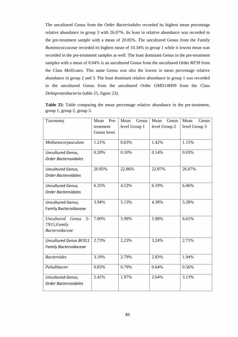
85

The uncultured Genus from the Order Bacteriodales recorded its highest mean percentage

relative abundance in group 3 with 26.07%. Its least in relative abundance was recorded in

the pre-treatment sample with a mean of 20.85%. The uncultured Genus from the Family

Ruminococcaceae recorded its highest mean of 10.34% in group 1 while it lowest mean was

recorded in the pre-treatment samples as well. The least dominant Genus in the pre-treatment

samples with a mean of 0.04% is an uncultured Genus from the uncultured Order RF39 from

the Class Mollicutes. This same Genus was also the lowest in mean percentage relative

abundance in group 2 and 3. The least dominant relative abundance in group 1 was recorded

in the uncultured Genus from the uncultured Order GMD14H09 from the Class

Deltaproteobacteria (table 25, figure 23).

Table 25: Table comparing the mean percentage relative abundance in the pre-treatment,

group 1, group 2, group 3.

Taxonomy Mean Pre-

treatment

Genus level.

Mean Genus

level Group 1

Mean Genus

level Group 2

Mean Genus

level Group 3


Uncultured Genus,


0.20% 0.10% 0.14% 0.03%

Uncultured Genus,

Order Bacteroidales

20.85% 22.86% 22.87% 26.07%

Uncultured Genus,

Order Bacteroidales

6.35% 4.53% 6.19% 6.46%

Uncultured Genus,


3.94% 5.13% 4.38% 5.28%

Uncultured Genus 5-

7N15,Family

Bacteroidaceae

7.00% 5.99% 5.98% 6.61%



2.73% 2.23% 3.24% 2.71%

Bacteroides 3.19% 2.79% 2.83% 1.94%

Paludibacter 0.83% 0.79% 0.64% 0.56%

Uncultured Genus,


2.42% 1.97% 2.64% 3.13%

86

Uncultured Genus,


5.65% 5.61% 5.01% 5.85%

Uncultured Genus

CF231, Family

Paraprevotellaceae

2.65% 2.94% 2.46% 2.79%

Uncultured Genus

YRC22 Family

Paraprevotellaceae

1.16% 0.97% 0.67% 1.25%

[Prevotella] 0.11% 0.25% 0.21% 0.07%

Uncultured Genus,


1.17% 1.08% 1.28% 0.36%

Fibrobacter 4.65% 5.73% 7.12% 2.28%

Uncultured Genus,

Order Clostridiales

6.57% 6.56% 5.80% 5.62%

Uncultured Genus,

Family

Christensenellaceae

0.57% 0.38% 0.33% 0.33%

Clostridium 7.01% 8.09% 6.21% 7.67%

Uncultured Genus,

Family Lachnospiraceae

3.59% 3.18% 2.47% 2.42%


4,Family

Peptococcaceae

0.36% 0.29% 0.28% 0.21%

Uncultured Genus,

Family

Ruminococcaceae

9.60% 10.34% 9.03% 10.14%

Ruminococcus 0.19% 0.35% 0.23% 0.08%


Uncultured Genus,

Family

Desulfovibrionaceae

0.31% 0.25% 0.22% 0.22%


Deltaproteobacteria

0.24% 0.07% 0.12% 0.06%

87

Campylobacter 1.89% 1.17% 1.57% 1.22%

Treponema 2.17% 2.75% 3.20% 2.05%


Mollicutes

0.04% 0.25% 0.05% 0.01%


Verruco-5

0.20% 0.11% 0.22% 0.55%

Akkermansia 1.97% 1.46% 1.99% 1.87%

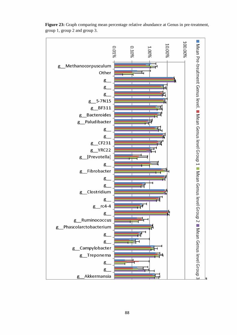
88

Figure 23: Graph comparing mean percentage relative abundance at Genus in pre-treatment,

group 1, group 2 and group 3.

s

89

4.5 Rarefaction Curves. Species richness (α-diversity) in both pre-treatment and post-treated samples was measured

by the use of rarefaction curve. A rarefaction curve is a plot of the number of species as a

function of the number of samples. It is determined by scaling down the number of

sequences to the same number in all the samples and determining the number of species in

the standardized sequences within each sample. Rarefaction is expressed statistically as

E(Sn) where n is the expected number of species in a standardized sequence from a larger

sample sequence N. Alpha rarefaction was performed using the QIIME pipeline.

The gradient of a rarefaction curve determines the species richness of a sample. The steeper

the gradient, the greater the species richness (alpha-diversity) in the sample. Figure 24

represents the rarefaction curve of the pre-treatment samples and the post-treated samples

with pre-treatment outliers and post treated outliers performed with QIIME. The post treated

samples (red curve) have a slightly higher gradient than the pre-treatment samples (orange)

indicating that they might have a slightly higher species richness than the pre-treated

samples. The post-treated outliers (blue) have a higher gradient than the pre-treated outliers

(green) indicating there is more alpha diversity in the post-treated outliers than the pre-

treated outliers.

There was no significant difference between the post treated group (red) and the pre-

treatment group (orange) with P = 1 and a t value of -1.33. The post treated group (Red) and

the post treated outliers (blue) were significantly different with P = 0.006 and a t value of

3.10. The post treated group (red) and the pre-treatment outliers (green) were also

significantly different with a P value of 0.006 and a t value of 8.81. The pre-treatment group

(orange) and the post treated outliers (blue) were not significantly different with a P = 0.672

and t = 1.57. The pre-treatment group (orange) and the pre-treatment outliers were

significantly different with a P value of 0.006 a t value of 5.50. The pre-treatment outliers

(green) and the post treated outliers (blue) were also significantly different with P = 0.01 and

t = 3.96.

90

Figure 24: Rarefaction curve of pre-treatment, post-treated samples with pre-treated and

post-treated outliers.

91

4.6 Shannon – diversity Index Shannon diversity is a statistical tool that measures alpha diversity and the proportion of the

distribution of each species within the sample. Samples high in species richness that are

more evenly distributed will have a higher Shannon diversity index than samples with low

species richness being less evenly distributed.

Figure 25 represents the Shannon diversity index of the pre-treatment and post treated

samples and their outliers. The post-treated sample has a higher Shannon diversity index

which means it is higher in species richness with the species more evenly distributed than the

other samples. The pre-treated sample outlier is the lowest in Shannon diversity index which

means it has the lowest species richness that are less evenly distributed.

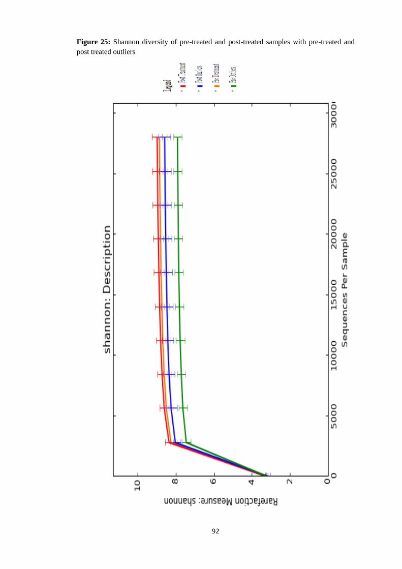
92

Figure 25: Shannon diversity of pre-treated and post-treated samples with pre-treated and

post treated outliers

93

4.7 Metric Multidimensional Scaling Analysis.

Similarity or resemblance between the pre-treatment and post-treated samples was measured

using the Bray – Curtis statistical tool based on the relative abundance of the OTUs in each

of the samples. Bray – Curtis similarity matrices was use to generate non – metric

multidimensional plots that show similarity or resemblance between the pre-treatment and

post-treated samples in a 2dimensional view. Factors namely Pre-treatment, S (Startect®,

same as group 2), Z+S (Zolvix® + Startec®t, same as group 3), Z (Zolvix® same as group

1) was use to generate the Bray - Curtis similarity curve. The Pre-treatment factor colour

coded green triangle represents barcodes 21-60 (38 samples), the Factor S colour coded blue

inverted triangle represents all the samples treated with Startect® that is group 2 (12

samples), the factor Z colour coded red rhombus represents samples treated with Zolvix®

that is group 1 (15 samples), while factor Z+S colour coded blue square represents samples

treated with a combination of Zolvix® plus Startect® that is group 3 (10 samples). The

Kruskal stress value which determines the fitness of the plot in the 2dimensional view was

0.18 which is within the acceptable range (stress < 0.2, if > 0.2 the plot is distorted).

Samples that resemble each other appear close together in the plot while samples that are not

similar are further apart from each other. There is a clustering together of most pre-treatment

samples with the post-treated samples. There is a clustering of post-treated samples (Z, S,

Z+S, that is group 1, 2 and 3). Most of the outliers appear in the pre-treated samples (23, 25,

32, 43, 45,47, 53).

From the statistical analysis by PERMANOVA, there was no significant difference between

the pre-treatment samples and the group 2 (Startect®) where P = 0.166 with a t value of

1.084. PERMANOVA revealed a marginal significance in differences between the pre-

treatment samples and the group 3 samples (Zolvix® + Startect®) with P = 0.052 and a t

value of 1.159. There was no significant difference between the pre-treatment samples and

group 1 (Zolvix®) with a P value of 0.06 and a t value of 1.156. The difference in the group

2 (Startect®) and group 3 was also not significant with P = 0.206 and t = 1.0535. Again

PERMANOVA also revealed no difference between the group 1 (Zolvix®) and the group 2

(Startect®) with P value of 0.161 and a t value of 1.0593. There was a significant difference

94

between the group 3 (Zolvix® + Startect®) and the group 1 (Zolvix®) with P = 0.01 and t

= 1.169 (table 26a).

Table 26a: PERMANOVA results of pre-treatment and post treatment pairwise with

outliers.

Groups t value P (perm) Unique perms

Pre-treatment, group 2

(Startect®)

1.0841 0.166 997


(Zolvix®+Startect®)

1.1599 0.052 998


(Zolvix®)

1.1564 0.06 994

Group2 (Startect®),

group3

(Zolvix®+Startect®)

1.0535 0.206 996

Group2 (Startect®),

Group1 (Zolvix®)

1.0593 0.161 997

Group3

(Zolvix®+Startect®),

Group 1 (Zolvix®).

1.1686 0.01 996

95

Figure 26a: Bray – Curtis MDS plot based on relative abundance of OTUs for pre-treatment

and post-treated samples (S, Z+S, Z) revealing outliers.

96

An MDS was again plotted to further view the relationship of the different groups without

the pre-treatment outliers. This was performed so as to view with a bit of details the Bray-

Curtis similarity curve (Figure 26b). PERMANOVA pair wise test revealed without the

outliers revealed no significant difference between the clustering of the pre-treatment

samples and the group 2 (Startect®),) with a P value of 0.221 and a t value of 1.046. It

revealed a significant difference between the clustering of pre-treatment samples and group 3

(Zolvix®), plus Startect®),) with P = 0.01 and t = 1.210. There was no significant

difference between the clustering of pre-treatment samples and group 1 (Zolvix®),) with P

= 0.111 and t = 1.098. It also showed no significant difference between the clustering of

group 2 (Startect®),) and group 3 (Zolvix®), plus Startect®),) P value of 0.167 t value of

1.053. Again there was no significant difference between the clustering of group 2

(Startect®),) and group 1 (Zolvix®),) P = 0.161 and t = 1.059. But it revealed a significant

difference between the clustering of Group 1(Zolvix®),) and Group 3 (Zolvix®), plus

Startect®) with a P value of 0.012 and a t value of 1.168 (table 26b).

Table 26b: PERMANOVA results of pre-treatment and post treatment pairwise without

outliers.

Groups t value P (perm) Unique perms


(Startect®)

1.046 0.221 995


(Zolvix+Startect®)

1.210 0.01 997

Pre-treatment group 1

(Zolvix®)

1.098 0.111 996

Group 2 (Startect®), group

3 (Zolvix®),+Startect®)

1.053 0.167 995

Group 2 (Startect®), Group 1.059 0.161 996

97

1 (Zolvix®)

Group 3

(Zolvix®)+Startect®),Group

1 (Zolvix®).

1.168 0.012 996

98

Figure 26b: Bray – Curtis MDS plot based on relative abundance of OTUs for pre-treatment

and post-treated samples (S, Z+S, Z) without outliers. Annotation of data is the sample

Barcode.

99

4.7.1 Statistical View of Outliers at Order level. From the MDS plot in Figure 26a, it is observed that some of the pre – treatment samples

appeared as outliers. The barcodes that appear as outliers include BC25, BC32, BC23, BC45,

BC53, BC47, and BC43.

Methanomicrobiales had a mean percentage relative of 2.07% in the pre – treatment outliers.

Bacteroidales which was the most dominant had a mean percentage relative abundance of

54.06% followed by the Order Clostridiales with a mean of 31.51%. Campylobacterales

recorded a mean percentage relative abundance of 5.79%. The least dominant was the

uncultured Order RF39 from the Class Mollicutes with a mean of 0.01%.

Table 27: Mean percentage relative abundance in Pre – treatment outliers.

Taxonomy Mean Pre - treatment

outliers

Standard deviation

outliers.






GMD14H09 0.61% 1.58%



Uncultured Order

RF39, Class

Mollicutes

0.01% 0.04%

Uncultured Order

WCHB1-41, Class

Verucco-5

0.23% 0.44%


100

Figure 27: Graph representing the mean percentage relative abundance in the pre – treatment

outliers at Order level of Taxonomy.

The Order Bacteroidales was most dominant in group 3. The Order Clostridiales were most

dominant in the outliers with a mean of 31.51%. The uncultured Order RF39 from the Class

Mollicutes was least in both the pre-treatment outliers and Group 3 (Table 28, Figure 28).

Table 28: Mean percentage relative abundance in pre – treatment outliers, Group 1

(Zolvix®), Group 2 (Startect®), Group 3 (Zolvix® + Startect®).

Taxonomy Mean Pre -

treatment

outliers

Mean Group 1 Mean Group 2 Mean Group

3


Bacteroidales 54.06% 57.25% 58.56% 63.13%


Clostridiales 31.51% 30.34% 25.53% 27.43%


0.01%

0.10%

1.00%

10.00%

100.00%

Mean Pre - treatment outliers Mean Pre - treatment outliers

101

Uncultured Order,

GMD14H09 Class

Deltaproteobacteria

0.61% 0.07% 0.12% 0.06%


Spirochaetales 1.21% 2.75% 3.20% 2.05%

Uncultured Order

RF39,Class

Mollicutes

0.01% 0.25% 0.05% 0.01%

Uncultured Order

WCHB1-41,Class

Verruco-5

0.23% 0.11% 0.22% 0.55%


Figure 28: Graph comparing mean percentage relative abundance in pre – treatment outliers,

group1, group 2 and group 3 at Order level of Taxonomy.

0.01%

0.10%

1.00%

10.00%

100.00%

Mean Treatment Outliers Mean Group 1 (Zolvix)

Mean Group 2 (Startect) Mean Group 3 (Zolvix + Startect)

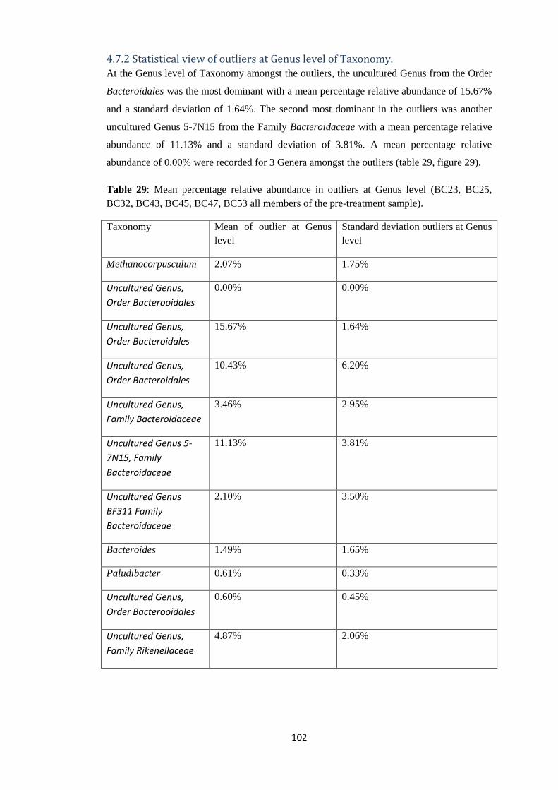
102

4.7.2 Statistical view of outliers at Genus level of Taxonomy. At the Genus level of Taxonomy amongst the outliers, the uncultured Genus from the Order

Bacteroidales was the most dominant with a mean percentage relative abundance of 15.67%

and a standard deviation of 1.64%. The second most dominant in the outliers was another

uncultured Genus 5-7N15 from the Family Bacteroidaceae with a mean percentage relative

abundance of 11.13% and a standard deviation of 3.81%. A mean percentage relative

abundance of 0.00% were recorded for 3 Genera amongst the outliers (table 29, figure 29).

Table 29: Mean percentage relative abundance in outliers at Genus level (BC23, BC25,

BC32, BC43, BC45, BC47, BC53 all members of the pre-treatment sample).

Taxonomy Mean of outlier at Genus

level

Standard deviation outliers at Genus

level


Uncultured Genus,


0.00% 0.00%

Uncultured Genus,

Order Bacteroidales

15.67% 1.64%

Uncultured Genus,

Order Bacteroidales

10.43% 6.20%

Uncultured Genus,


3.46% 2.95%

Uncultured Genus 5-

7N15, Family

Bacteroidaceae

11.13% 3.81%

Uncultured Genus

BF311 Family

Bacteroidaceae

2.10% 3.50%



Uncultured Genus,


0.60% 0.45%

Uncultured Genus,


4.87% 2.06%

103

Uncultured Genus

CF231, Family

Paraprevotellaceae

2.07% 1.49%

Uncultured Genus

YRC22 Family

Paraprevotellaceae

1.60% 1.97%


Uncultured Genus,


0.00% 0.00%


Uncultured Genus,

Order Clostridiales

4.71% 0.63%

Uncultured Genus,

Family

Christensenellaceae

1.81% 1.75%


Uncultured Genus,

Family

Lachnospiraceae

4.11% 3.23%


4, Family

Peptococcaceae

0.84% 0.52%

Uncultured Genus,

Family

Ruminococcaceae

10.67% 3.16%



Uncultured Genus,

Family

Desulfovibrionaceae

0.64% 0.56%

Uncultured Genus,

Class

Deltaproteobacteria

0.61% 1.58%

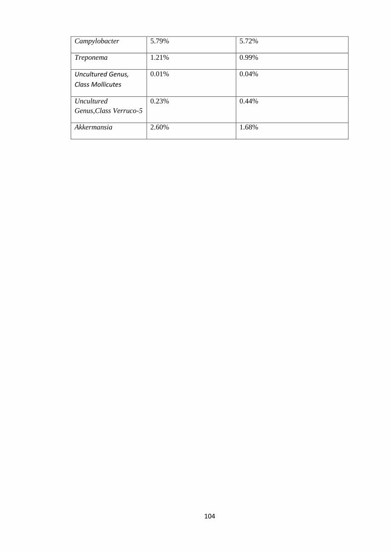
104



Uncultured Genus,

Class Mollicutes

0.01% 0.04%

Uncultured

Genus,Class Verruco-5

0.23% 0.44%


105

Figure 29: Graph of mean percentage relative abundance at Genus level in pre-treatment

outliers.

106

The uncultured Genus from the Order Bacteroidales recorded the highest mean percentage

relative abundance of 26.07% in group 3 while its lowest was recorded in the pre- treatment

outliers. A mean percentage relative abundance of 0.00% was seen in 3 Genera in the pre-

treatment outliers. Another uncultured Genus 5-7N15 from the Family Bacteroidaceae had a

mean percentage relative abundance of 11.13% in the pre-treatment outliers which was

higher than what it recorded in all the other groups. Campylobacter recorded a mean

percentage relative abundance of 5.79% in the pre-treatment outliers which was higher than

what it recorded in the other samples (table 30, figure 30).

Table 30: Table comparing mean percentage relative abundance at Genus level in Group1

(Zolvix®), Group2 (Startect®), Group3 (Zolvix® + Startect®) and Pre-treatment

outliers.

Taxonomy Mean

Genus

level

Group 1

Mean Genus

level Group 2

Mean Genus

level Group 3

Mean of outlier

at Genus level


Uncultured Genus,


0.10% 0.14% 0.03% 0.00%

Uncultured Genus,

Order Bacteroidales

22.86% 22.87% 26.07% 15.67%

Uncultured Genus,

Order Bacteroidales

4.53% 6.19% 6.46% 10.43%

Uncultured Genus,


5.13% 4.38% 5.28% 3.46%

Uncultured Genus 5-

7N15, Family

Bacteroidaceae

5.99% 5.98% 6.61% 11.13%

Uncultured Genus

BF311 Family

Bacteroidaceae

2.23% 3.24% 2.71% 2.10%

Bacteroides 2.79% 2.83% 1.94% 1.49%

Paludibacter 0.79% 0.64% 0.56% 0.61%

Uncultured Genus, 1.97% 2.64% 3.13% 0.60%

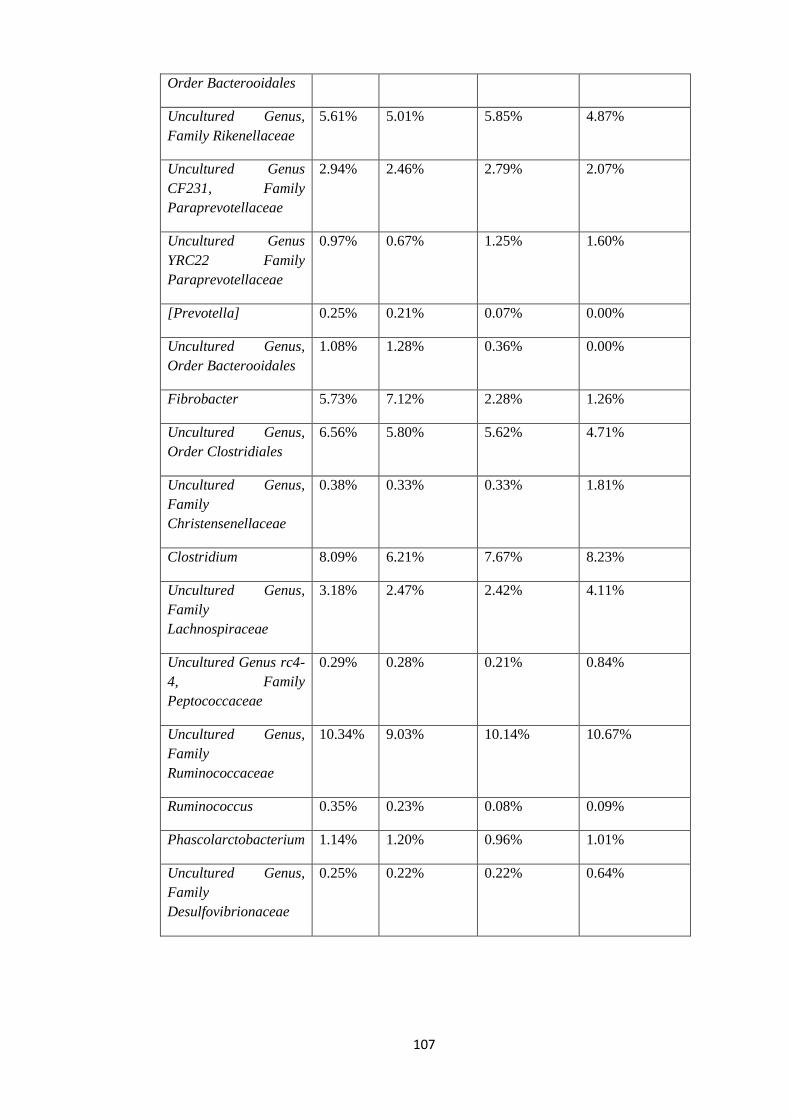
107


Uncultured Genus,


5.61% 5.01% 5.85% 4.87%

Uncultured Genus

CF231, Family

Paraprevotellaceae

2.94% 2.46% 2.79% 2.07%

Uncultured Genus

YRC22 Family

Paraprevotellaceae

0.97% 0.67% 1.25% 1.60%

[Prevotella] 0.25% 0.21% 0.07% 0.00%

Uncultured Genus,


1.08% 1.28% 0.36% 0.00%

Fibrobacter 5.73% 7.12% 2.28% 1.26%

Uncultured Genus,

Order Clostridiales

6.56% 5.80% 5.62% 4.71%

Uncultured Genus,

Family

Christensenellaceae

0.38% 0.33% 0.33% 1.81%

Clostridium 8.09% 6.21% 7.67% 8.23%

Uncultured Genus,

Family

Lachnospiraceae

3.18% 2.47% 2.42% 4.11%


4, Family

Peptococcaceae

0.29% 0.28% 0.21% 0.84%

Uncultured Genus,

Family

Ruminococcaceae

10.34% 9.03% 10.14% 10.67%

Ruminococcus 0.35% 0.23% 0.08% 0.09%


Uncultured Genus,

Family

Desulfovibrionaceae

0.25% 0.22% 0.22% 0.64%

108

Uncultured Genus,

Class

Deltaproteobacteria

0.07% 0.12% 0.06% 0.61%

Campylobacter 1.17% 1.57% 1.22% 5.79%

Treponema 2.75% 3.20% 2.05% 1.21%

Uncultured Genus,

Class Mollicutes

0.25% 0.05% 0.01% 0.01%

Uncultured

Genus,Class Verruco-5

0.11% 0.22% 0.55% 0.23%

Akkermansia 1.46% 1.99% 1.87% 2.60%

109

Figure 30: Graph comparing mean percentage relative abundance in Group1, Group2,

Group3 and Pre-treatment outliers at Genus level of Taxonomy.

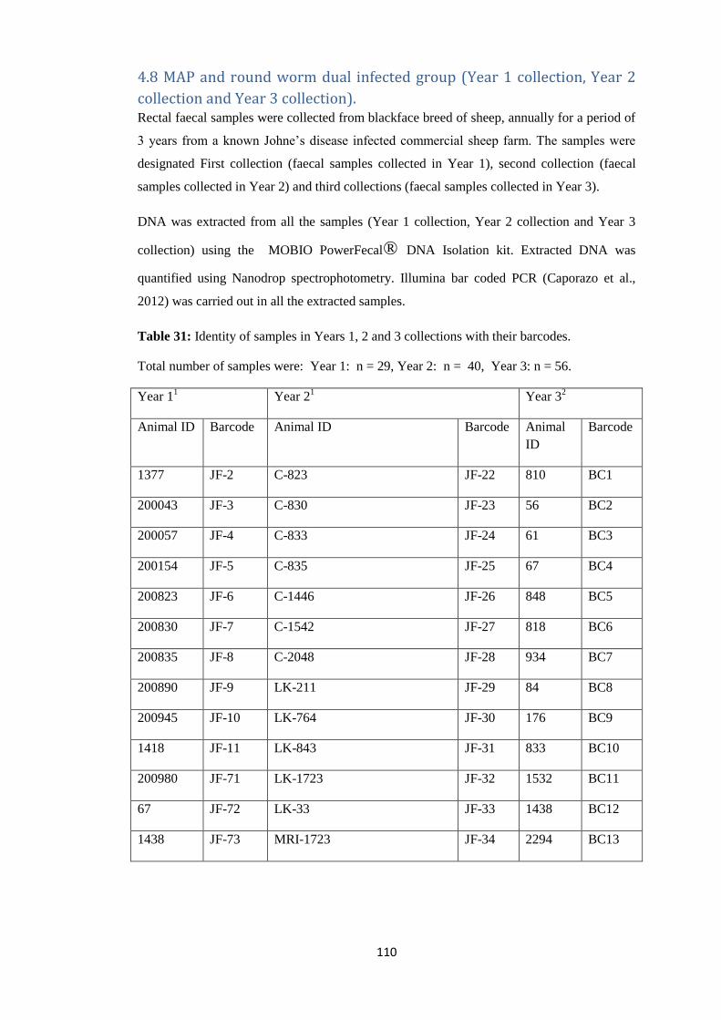
110

4.8 MAP and round worm dual infected group (Year 1 collection, Year 2

collection and Year 3 collection). Rectal faecal samples were collected from blackface breed of sheep, annually for a period of

3 years from a known Johne’s disease infected commercial sheep farm. The samples were

designated First collection (faecal samples collected in Year 1), second collection (faecal

samples collected in Year 2) and third collections (faecal samples collected in Year 3).

DNA was extracted from all the samples (Year 1 collection, Year 2 collection and Year 3

collection) using the MOBIO PowerFecal® DNA Isolation kit. Extracted DNA was

quantified using Nanodrop spectrophotometry. Illumina bar coded PCR (Caporazo et al.,

2012) was carried out in all the extracted samples.

Table 31: Identity of samples in Years 1, 2 and 3 collections with their barcodes.

Total number of samples were: Year 1: n = 29, Year 2: n = 40, Year 3: n = 56.

Year 11 Year 2

1 Year 3

2

Animal ID Barcode Animal ID Barcode Animal

ID

Barcode

1377 JF-2 C-823 JF-22 810 BC1

200043 JF-3 C-830 JF-23 56 BC2

200057 JF-4 C-833 JF-24 61 BC3

200154 JF-5 C-835 JF-25 67 BC4

200823 JF-6 C-1446 JF-26 848 BC5

200830 JF-7 C-1542 JF-27 818 BC6

200835 JF-8 C-2048 JF-28 934 BC7

200890 JF-9 LK-211 JF-29 84 BC8

200945 JF-10 LK-764 JF-30 176 BC9

1418 JF-11 LK-843 JF-31 833 BC10

200980 JF-71 LK-1723 JF-32 1532 BC11

67 JF-72 LK-33 JF-33 1438 BC12

1438 JF-73 MRI-1723 JF-34 2294 BC13

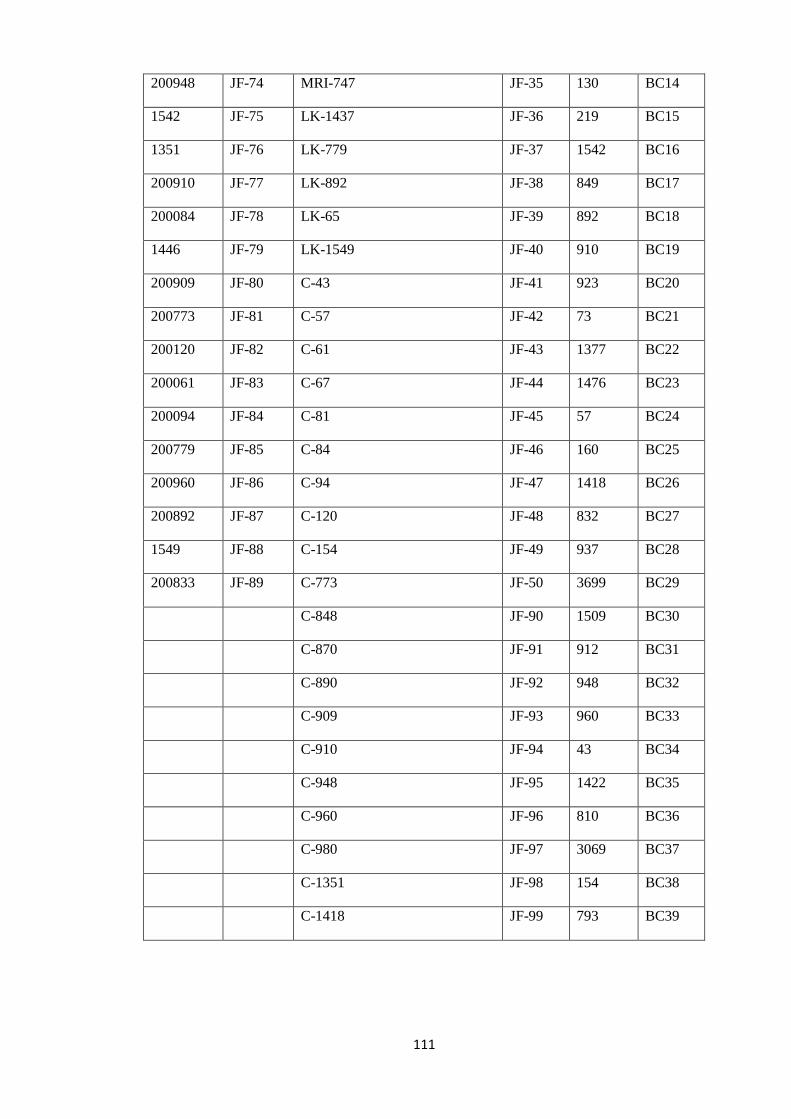
111

200948 JF-74 MRI-747 JF-35 130 BC14

1542 JF-75 LK-1437 JF-36 219 BC15

1351 JF-76 LK-779 JF-37 1542 BC16

200910 JF-77 LK-892 JF-38 849 BC17

200084 JF-78 LK-65 JF-39 892 BC18

1446 JF-79 LK-1549 JF-40 910 BC19

200909 JF-80 C-43 JF-41 923 BC20

200773 JF-81 C-57 JF-42 73 BC21

200120 JF-82 C-61 JF-43 1377 BC22

200061 JF-83 C-67 JF-44 1476 BC23

200094 JF-84 C-81 JF-45 57 BC24

200779 JF-85 C-84 JF-46 160 BC25

200960 JF-86 C-94 JF-47 1418 BC26

200892 JF-87 C-120 JF-48 832 BC27

1549 JF-88 C-154 JF-49 937 BC28

200833 JF-89 C-773 JF-50 3699 BC29

C-848 JF-90 1509 BC30

C-870 JF-91 912 BC31

C-890 JF-92 948 BC32

C-909 JF-93 960 BC33

C-910 JF-94 43 BC34

C-948 JF-95 1422 BC35

C-960 JF-96 810 BC36

C-980 JF-97 3069 BC37

C-1351 JF-98 154 BC38

C-1418 JF-99 793 BC39

112

C-1438 JF-100 800 BC40

823 BC41

830 BC42

1542 BC43

1619 BC44

1477 BC45

3136 BC46

2363 BC47

1446 BC48

3685 BC49

1433 BC50

834 BC51

835 BC52

1503 BC53

2401 BC54

1453 BC55

3685 BC56

1 samples extracted, PCR generated by Jelena Nikolić, 2014 and Miriam Navarro, 2015

and sequenced by Dr Craig Watkins; 2 samples extracted, PCR generated and

sequenced by Swang Shallangwa 2015-16

113

Figure 31: Ultraviolet Image of PCR products shown by gel electrophoresis for third

collection (Year3).

Figure 28 illustrates examples of the ultraviolet images that were obtained after gel

electrophoresis of the PCR products. As can be seen from the image, there was no band

obtained in well 13 which corresponded to BC33. The PCR was repeated for BC33 which

later on revealed a band after imaging.

4.8.1 Analysis of Bacterial and archael community. Following DNA extraction and amplification of the 16SrRNA gene V4 region by PCR , 29

Year 1, 40 Year 2 and 56 Year 3 collections making a total of 125 samples were chosen and

forwarded to the Edinburgh Genomics for sequencing through the use of Illumina MiSeq

platform.

4.8.2 QIIME Taxonomy Results The data obtained from Edinburgh Genomics was analysed by using the QIIME pipeline. An

output file of 10,066,725 sequences was obtained after chimeras were filtered out. The

complete QIIME pipeline analysis was performed, including the PyNast alignment with the

Lane Bar

code

100BP BP

1 0

2 23

3 24

4 25

5 26

6 27

7 28

8 29

9 30

10 31

11 32

12 33

114

Greengenes 13_8 databases. An OTU table excluding the PyNast failures was created.

Singletons were also filtered out (164,907 OTUs) from the overall sequence data sets.

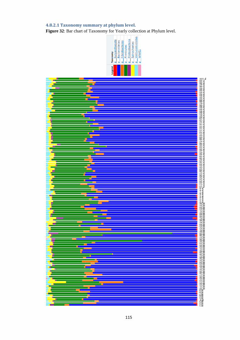
115

4.8.2.1 Taxonomy summary at phylum level.

Figure 32: Bar chart of Taxonomy for Yearly collection at Phylum level.

116

In the Year 1 collection at the Phylum level of taxonomy, a mean of 67.94% and a standard

deviation of 4.27% was recorded for Bacteroidetes, making it the Phylum with the highest

mean relative abundance in the Year 1 collection. Firmicutes was a distant second with a

mean relative abundance of 25.25% and a standard deviation of 3.52%. Fibrobacteres had a

mean relative abundance of 2.28% while Spirochaetes and Verrucomicrobia had a

percentage mean relative abundance of 1.89% and 1.88% respectively (Table 32, Figure 33

and Figure 32).

Table 32: Mean percentage of relative abundance at Phylum level, for Year 1 collection.

Taxonomy (Phylum) Mean Relative Abundance

– Year 1 collection

Standard deviation -

Year 1 Collection








Uncultured Phylum WWE1 0.00% 0.00%

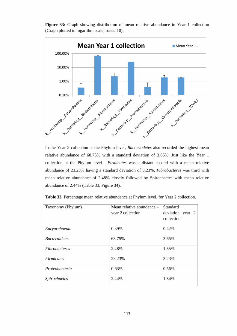
117

Figure 33: Graph showing distribution of mean relative abundance in Year 1 collection

(Graph plotted in logarithm scale, based 10).

In the Year 2 collection at the Phylum level, Bacteriodetes also recorded the highest mean

relative abundance of 68.75% with a standard deviation of 3.65%. Just like the Year 1

collection at the Phylum level. Firmicutes was a distant second with a mean relative

abundance of 23.23% having a standard deviation of 3.23%. Fibrobacteres was third with

mean relative abundance of 2.48% closely followed by Spirochaetes with mean relative

abundance of 2.44% (Table 33, Figure 34).

Table 33: Percentage mean relative abundance at Phylum level, for Year 2 collection.

Taxonomy (Phylum) Mean relative abundance –

year 2 collection

Standard

deviation year 2

collection







0.10%

1.00%

10.00%

100.00%

Mean Year 1 collection Mean Year 1 …

118



Figure 34: Graph showing mean percentage relative abundance for year 2 Collection (Graph

plotted in logarithm scale base 10).

In the Year 3 collection at the Phylum level, we also see Bacteriodetes with the highest mean

percentage relative abundance of 66.35% having a standard deviation of 10.48%. Like the

first and second collection Firmicutes was a distant second in the third collection with a

mean of 24.45% and a standard deviation of 10.06%. Fibrobacteres had a mean percentage

relative abundance of 3.52% (Table 34, Figure 35).

Table 34: Percentage mean relative abundance Phylum level Year 3 collection.

Taxonomy (Phylum) Mean relative abundance

- year 3 Collection

Standard Deviation

year 3 Collection







0.10%

1.00%

10.00%

100.00%

Mean year 2 collection Mean year 2 collection

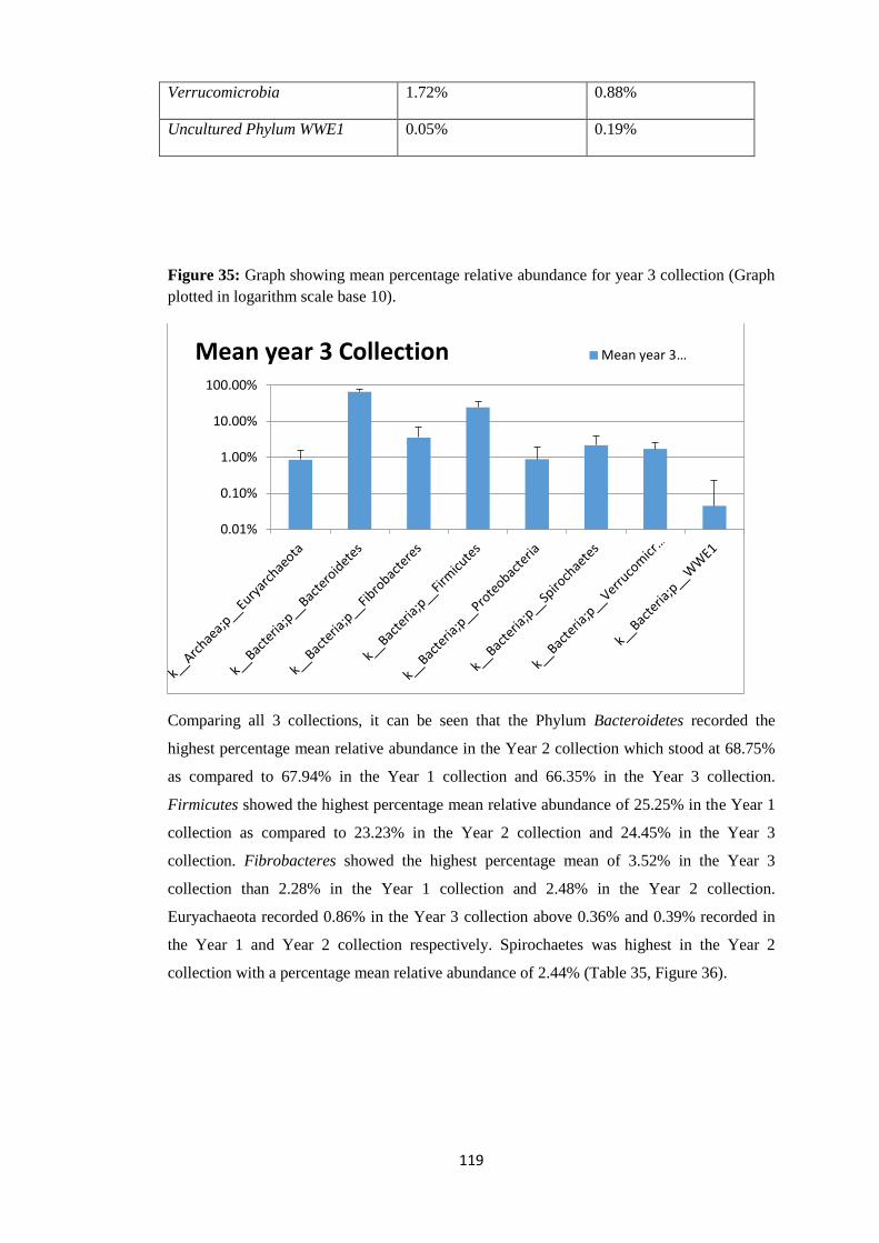
119



Figure 35: Graph showing mean percentage relative abundance for year 3 collection (Graph

plotted in logarithm scale base 10).

Comparing all 3 collections, it can be seen that the Phylum Bacteroidetes recorded the

highest percentage mean relative abundance in the Year 2 collection which stood at 68.75%

as compared to 67.94% in the Year 1 collection and 66.35% in the Year 3 collection.

Firmicutes showed the highest percentage mean relative abundance of 25.25% in the Year 1

collection as compared to 23.23% in the Year 2 collection and 24.45% in the Year 3

collection. Fibrobacteres showed the highest percentage mean of 3.52% in the Year 3

collection than 2.28% in the Year 1 collection and 2.48% in the Year 2 collection.

Euryachaeota recorded 0.86% in the Year 3 collection above 0.36% and 0.39% recorded in

the Year 1 and Year 2 collection respectively. Spirochaetes was highest in the Year 2

collection with a percentage mean relative abundance of 2.44% (Table 35, Figure 36).

0.01%

0.10%

1.00%

10.00%

100.00%

Mean year 3 Collection Mean year 3 …

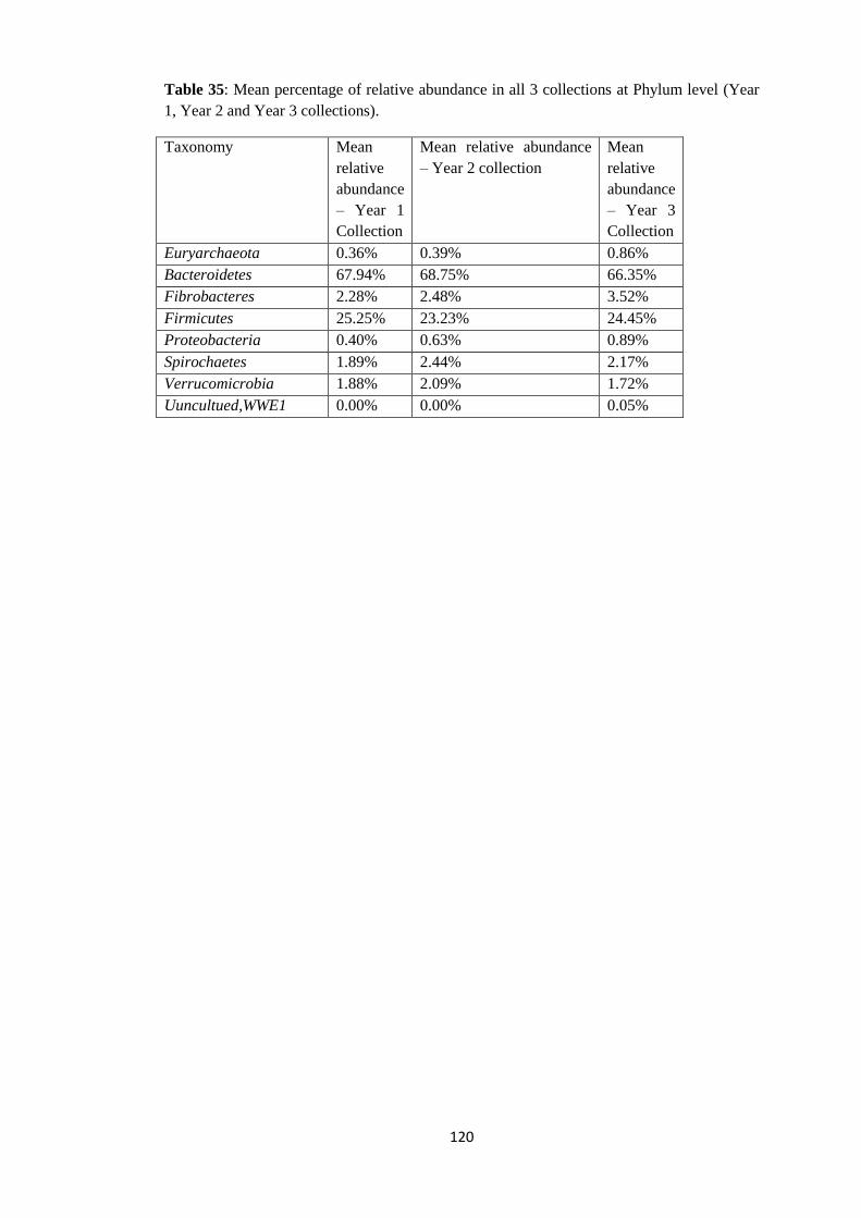
120

Table 35: Mean percentage of relative abundance in all 3 collections at Phylum level (Year

1, Year 2 and Year 3 collections).

Taxonomy Mean

relative

abundance

– Year 1

Collection

Mean relative abundance

– Year 2 collection

Mean

relative

abundance

– Year 3

Collection

Euryarchaeota 0.36% 0.39% 0.86%

Bacteroidetes 67.94% 68.75% 66.35%

Fibrobacteres 2.28% 2.48% 3.52%

Firmicutes 25.25% 23.23% 24.45%

Proteobacteria 0.40% 0.63% 0.89%

Spirochaetes 1.89% 2.44% 2.17%

Verrucomicrobia 1.88% 2.09% 1.72%

Uuncultued,WWE1 0.00% 0.00% 0.05%

121

Figure 36: Graph showing mean percentage relative abundance in all collections at the

Phylum level (year 1, year 2 and year 3).

122

4.8.2.2 Taxonomy summary at Order level.

Figure 37: Bar chart of Taxonomy at Order level for Yearly Collection.

123

The percentage mean relative abundance of the Order Methanomicrobiales in the Year 1

collection was 0.36% with a standard deviation of 0.34%. The Order Bacteroidales had the

highest mean percentage relative abundance standing at 67.94% with a standard deviation of

4.27 amongst the Year 1 collection. The Order Clostridiales was a distant second in the Year

1 collection with a mean percentage relative abundance of 25.17% and a standard deviation

of 3.50%. The Order Fibrobacterales had a percentage mean relative abundance of 2.28%

with a standard deviation of 1.63%. Campylobacterales had percentage mean relative

abundance of 0.21%. The Order Bacillales had a percentage mean relative abundance of

0.02% (Table 36, Figure 38).

Table 36: Percentage mean relative abundance with standard deviation at Order level of year

1 collection.

Taxonomy (Order) Mean

year 1 collection

Standard deviation

year 1 collection




Bacillales 0.02% 0.04%


Erysipelotrichales 0.06% 0.09%

Uncultured Order Class

Alphaproteobacteria

0.00% 0.02%



Enterobacteriales 0.01% 0.09%

Pasteurellales 0.00% 0.00%

Uncultured Order PL-

11B10, Phylum

Spirochaetes

0.17% 0.22%


WCHB1-41 0.74% 0.72%

124


[Cloacamonales] 0.00% 0.00%

Figure 38: Graph showing percentage mean relative abundance at Order level in year 1

collection. (Graph plotted in logarithm scale base 10).

In the Year 2 collection the Order Methanomicrobiales had a percentage mean relative

abundance of 0.39% with a standard deviation of 0.42%. Just like in the Year 1 collection,

the Order Bacteroidales also maintained the highest percentage mean relative abundance in

the Year 2 with a mean of 68.75% and a standard deviation of 3.65%. Clostridiales was

second in percentage mean relative abundance at 23.15%. Fibrobacterales stood at a

percentage mean relative abundance of 2.48% with a standard deviation of 1.55%. The Order

Erysipelotrichales had a mean of 0.04% and a standard deviation of 0.06% in percentage

relative abundance. Spirochaetales had a percentage mean relative abundance of 2.14%

while Campylobacterales had a mean of 0.42% respectively. Verrumicrobiales had a

percentage mean relative abundance of 1.29% with a standard deviation of 0.54% (Table 37,

Figure 29).

0.00%

0.01%

0.10%

1.00%

10.00%

100.00%

Mean order level year 1 collection

125

Table 37: Mean percentage of relative abundance with standard deviation at Order level of

Year 2 Collection.

Taxonomy (Order) Mean Relative Abundance

– year 2 collection

Standard deviation

year 2 collection







Uncultured Order

from the Class

Alphaproteobacteria

0.01% 0.03%





Uncultured Order

PL-11B10, Phylum

Spirochaetes

0.31% 0.62%


Uncultured Order

WCHB1-41, Class

Verruco-5

0.80% 0.47%



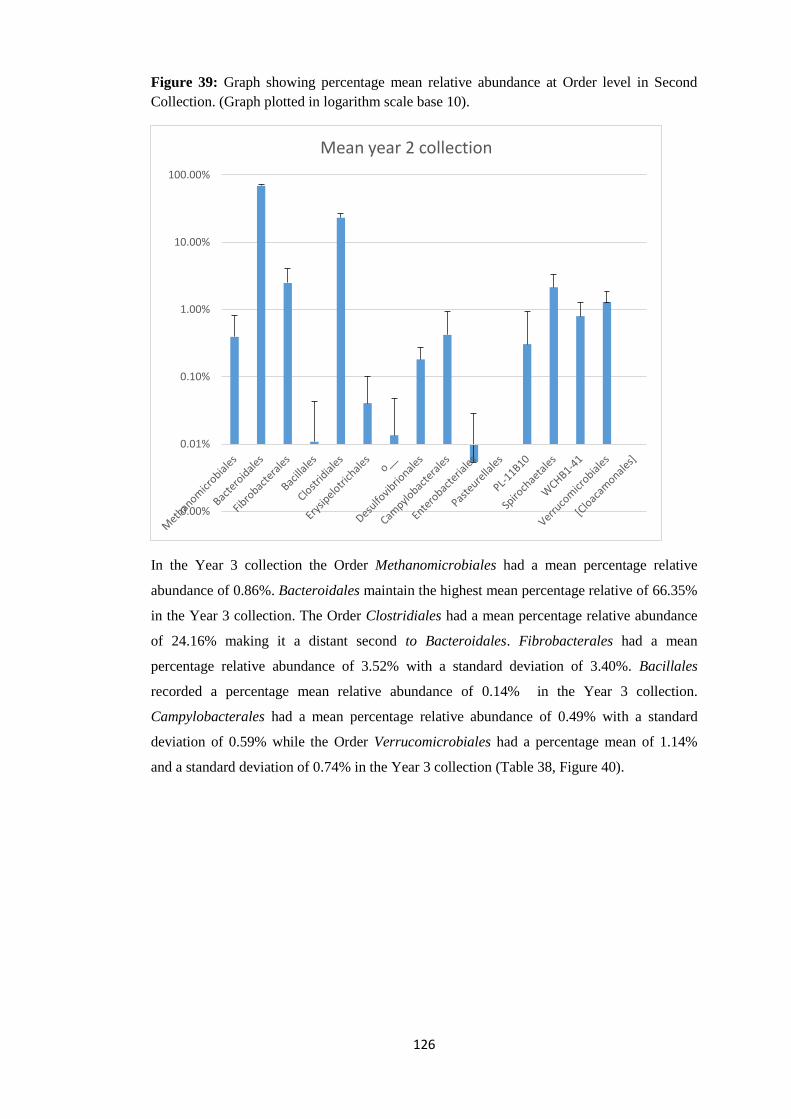
126

Figure 39: Graph showing percentage mean relative abundance at Order level in Second

Collection. (Graph plotted in logarithm scale base 10).

In the Year 3 collection the Order Methanomicrobiales had a mean percentage relative

abundance of 0.86%. Bacteroidales maintain the highest mean percentage relative of 66.35%

in the Year 3 collection. The Order Clostridiales had a mean percentage relative abundance

of 24.16% making it a distant second to Bacteroidales. Fibrobacterales had a mean

percentage relative abundance of 3.52% with a standard deviation of 3.40%. Bacillales

recorded a percentage mean relative abundance of 0.14% in the Year 3 collection.

Campylobacterales had a mean percentage relative abundance of 0.49% with a standard

deviation of 0.59% while the Order Verrucomicrobiales had a percentage mean of 1.14%

and a standard deviation of 0.74% in the Year 3 collection (Table 38, Figure 40).

0.00%

0.01%

0.10%

1.00%

10.00%

100.00%

Mean year 2 collection

127

Table 38: Percentage mean relative abundance with standard deviation at Order level of

Year 3 Collection.

Taxonomy (Order) Mean relative abundance

year 3 collection

Standard deviation

year 3 collection.







Uncultured Order

Class

Alphaproteobacteria

0.08% 0.47%





Uncultured Order PL-

11B10, Phylum

Spirochaetes

0.21% 0.39%


Uncultured Order

WCHB1-41Class

Verruco-5

0.58% 0.50%



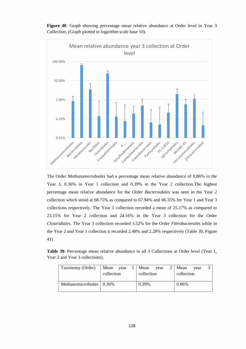
128

Figure 40: Graph showing percentage mean relative abundance at Order level in Year 3

Collection. (Graph plotted in logarithm scale base 10).

The Order Methanomicrobiales had a percentage mean relative abundance of 0.86% in the

Year 3, 0.36% in Year 1 collection and 0.39% in the Year 2 collection.The highest

percentage mean relative abundance for the Order Bacteroidales was seen in the Year 2

collection which stood at 68.75% as compared to 67.94% and 66.35% for Year 1 and Year 3

collections respectively. The Year 1 collection recorded a mean of 25.17% as compared to

23.15% for Year 2 collection and 24.16% in the Year 3 collection for the Order

Clostridiales. The Year 3 collection recorded 3.52% for the Order Fibrobacterales while in

the Year 2 and Year 1 collection it recorded 2.48% and 2.28% respectively (Table 39, Figure

41)

Table 39: Percentage mean relative abundance in all 3 Collections at Order level (Year 1,

Year 2 and Year 3 collections).

Taxonomy (Order) Mean year 1

collection

Mean year 2

collection

Mean year 3

collection

Methanomicrobiales 0.36% 0.39% 0.86%

0.01%

0.10%

1.00%

10.00%

100.00%

Mean relative abundance year 3 collection at Order level

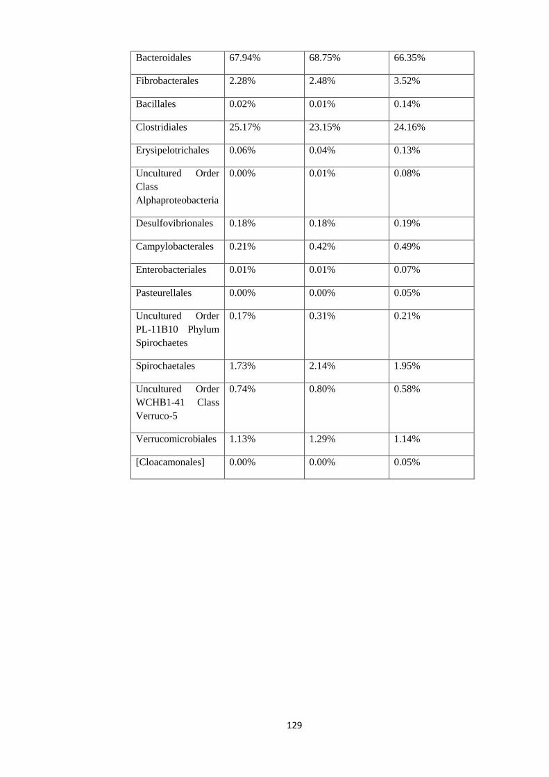
129

Bacteroidales 67.94% 68.75% 66.35%

Fibrobacterales 2.28% 2.48% 3.52%

Bacillales 0.02% 0.01% 0.14%

Clostridiales 25.17% 23.15% 24.16%

Erysipelotrichales 0.06% 0.04% 0.13%

Uncultured Order

Class

Alphaproteobacteria

0.00% 0.01% 0.08%

Desulfovibrionales 0.18% 0.18% 0.19%

Campylobacterales 0.21% 0.42% 0.49%

Enterobacteriales 0.01% 0.01% 0.07%

Pasteurellales 0.00% 0.00% 0.05%

Uncultured Order

PL-11B10 Phylum

Spirochaetes

0.17% 0.31% 0.21%

Spirochaetales 1.73% 2.14% 1.95%

Uncultured Order

WCHB1-41 Class

Verruco-5

0.74% 0.80% 0.58%

Verrucomicrobiales 1.13% 1.29% 1.14%

[Cloacamonales] 0.00% 0.00% 0.05%

130

Figure 41: Graph showing mean percentage relative abundance in all year 1, year 2 and year

3 collections. (Graph plotted in logarithm scale base 10). Data which is ≤0.01 is not plotted

on this graph due to log10 conversion on the y-axis.

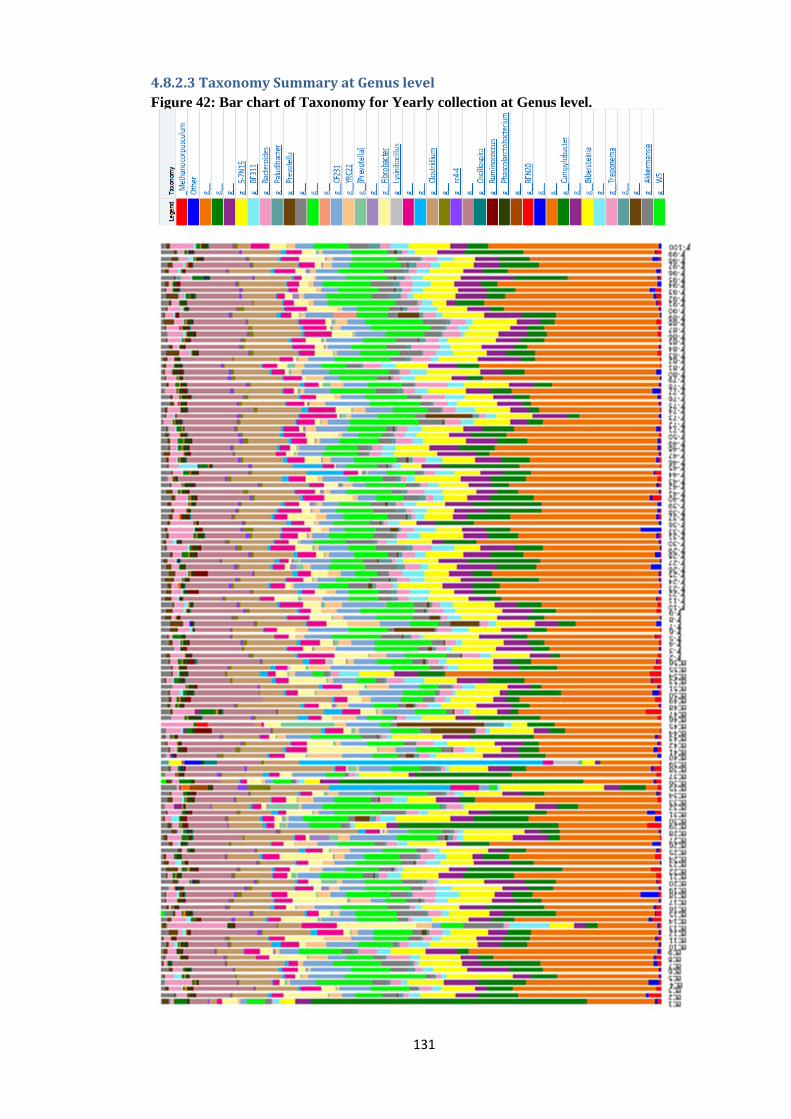
131

4.8.2.3 Taxonomy Summary at Genus level

Figure 42: Bar chart of Taxonomy for Yearly collection at Genus level.

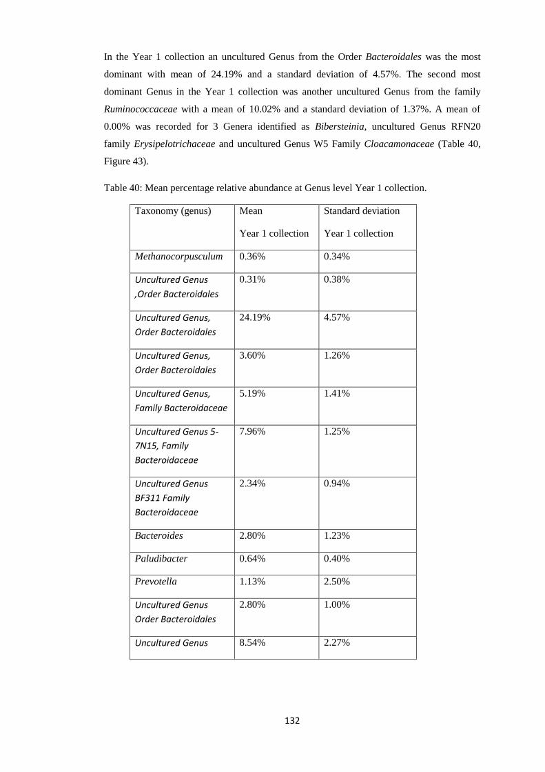
132

In the Year 1 collection an uncultured Genus from the Order Bacteroidales was the most

dominant with mean of 24.19% and a standard deviation of 4.57%. The second most

dominant Genus in the Year 1 collection was another uncultured Genus from the family

Ruminococcaceae with a mean of 10.02% and a standard deviation of 1.37%. A mean of

0.00% was recorded for 3 Genera identified as Bibersteinia, uncultured Genus RFN20

family Erysipelotrichaceae and uncultured Genus W5 Family Cloacamonaceae (Table 40,

Figure 43).

Table 40: Mean percentage relative abundance at Genus level Year 1 collection.

Taxonomy (genus) Mean

Year 1 collection

Standard deviation

Year 1 collection


Uncultured Genus

,Order Bacteroidales

0.31% 0.38%

Uncultured Genus,

Order Bacteroidales

24.19% 4.57%

Uncultured Genus,

Order Bacteroidales

3.60% 1.26%

Uncultured Genus,


5.19% 1.41%

Uncultured Genus 5-

7N15, Family

Bacteroidaceae

7.96% 1.25%

Uncultured Genus

BF311 Family

Bacteroidaceae

2.34% 0.94%



Prevotella 1.13% 2.50%

Uncultured Genus

Order Bacteroidales

2.80% 1.00%

Uncultured Genus 8.54% 2.27%

133


Uncultured Genus

Order Bacteroidales

0.16% 0.87%

Uncultured Genus

CF231 Family

Paraprevotellaceae

5.54% 1.45%

Uncultured Genus

YRC22 Family

Paraprevotellaceae

2.28% 1.36%


Uncultured Genus

Order Bacteroidales

0.11% 0.14%


Lysinibacillus 0.02% 0.04%

Uncultured Genus

Order Clostridiales

3.77% 1.37%

Uncultured Genus

Family

Christendenellaceae

0.41% 0.23%


Uncultured Genus

Family

Lachnospiraceae

0.58% 0.22%


4 Family

Peptococcaceae

0.33% 0.18%

Uncultured Genus

Family

Ruminococcaceae

10.02% 1.37%

Oscillospira 0.07% 0.08%

g__Ruminococcus 0.27% 0.23%


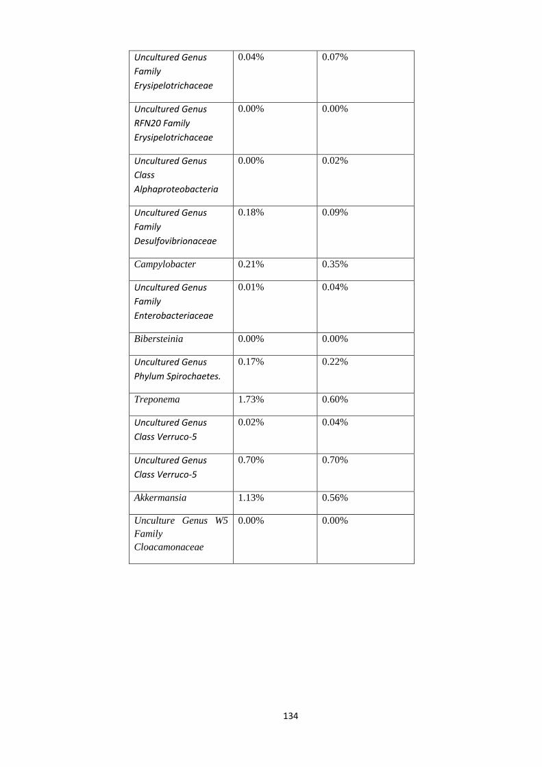
134

Uncultured Genus

Family

Erysipelotrichaceae

0.04% 0.07%

Uncultured Genus

RFN20 Family

Erysipelotrichaceae

0.00% 0.00%

Uncultured Genus

Class

Alphaproteobacteria

0.00% 0.02%

Uncultured Genus

Family

Desulfovibrionaceae

0.18% 0.09%


Uncultured Genus

Family

Enterobacteriaceae

0.01% 0.04%

Bibersteinia 0.00% 0.00%

Uncultured Genus

Phylum Spirochaetes.

0.17% 0.22%


Uncultured Genus

Class Verruco-5

0.02% 0.04%

Uncultured Genus

Class Verruco-5

0.70% 0.70%


Unculture Genus W5

Family

Cloacamonaceae

0.00% 0.00%

135

Figure 43: Graph representing mean percentage relative abundance in Year 1 collection at

Genus level.

136

The uncultured Genus from the Order Bacteroidales was the most dominant in relative

abundance with a mean of 28.11% and a standard deviation of 4.41% in the Year 2

collection. The second most dominant in relative abundance in the Year 2 collection was

another uncultured Genus from the family Ruminococcaceae with a mean of 9.12% and a

standard deviation of 1.58%. A mean percentage of 0.00% was recorded for 3 Genera

namely Biberteinia, an uncultured Genus from the Order Bacteroidale and another

uncultured Genus W5 from the Family Cloacamonceae (Table 41, Figure 44).


Taxonomy (Genus) Mean

year 2 collection

Standard deviation

year 2 collection


Uncultured Genus

Order Bacteroidales

0.59% 0.71%

Uncultured Genus

Order Bacteroidales

28.11% 4.41%

Uncultured Genus

Order Bacteroidales

6.91% 3.19%

Uncultured Genus


5.19% 1.64%

Uncultured Genus 5-

7N15 Family

Bacteroidaceae

6.31% 1.59%

Uncultured Genus

BF311 Family

Bacteroidaceae

2.59% 0.92%




Uncultured Genus

Order Bacteroidales

3.00% 1.32%

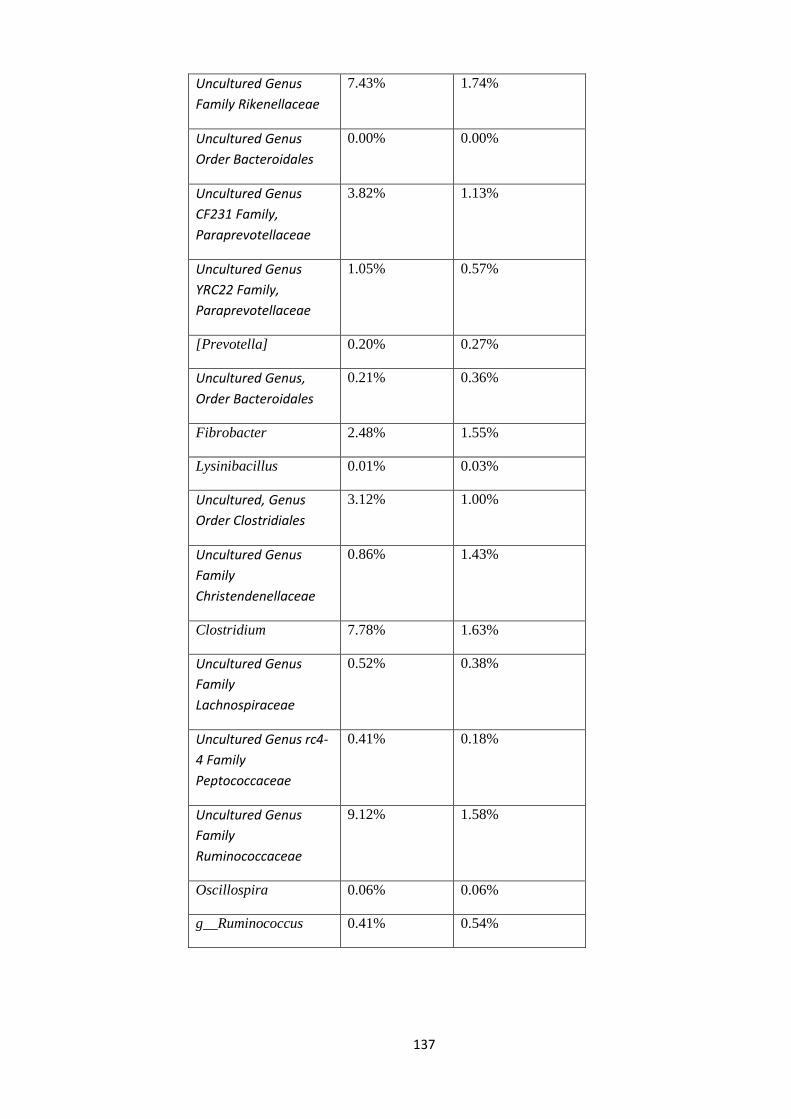
137

Uncultured Genus


7.43% 1.74%

Uncultured Genus

Order Bacteroidales

0.00% 0.00%

Uncultured Genus

CF231 Family,

Paraprevotellaceae

3.82% 1.13%

Uncultured Genus

YRC22 Family,

Paraprevotellaceae

1.05% 0.57%


Uncultured Genus,

Order Bacteroidales

0.21% 0.36%



Uncultured, Genus

Order Clostridiales

3.12% 1.00%

Uncultured Genus

Family

Christendenellaceae

0.86% 1.43%


Uncultured Genus

Family

Lachnospiraceae

0.52% 0.38%


4 Family

Peptococcaceae

0.41% 0.18%

Uncultured Genus

Family

Ruminococcaceae

9.12% 1.58%


g__Ruminococcus 0.41% 0.54%

138


Uncultured Genus

Family

Erysipelotrichaceae

0.02% 0.04%

Uncultured Genus

RFN20 Family

Erysipelotrichaceae

0.01% 0.04%

Uncultured Genus,

Class

Alphaproteobacteria

0.01% 0.03%

Uncultured Genus,

Family

Desulfovibrionaceae

0.18% 0.09%


Uncultured Genus,

Family

Enterobacteriaceae

0.01% 0.02%


Uncultured Genus


0.31% 0.62%


Uncultured Genus

Class Verruco-5

0.06% 0.15%

Uncultured Genus,

Class Verruco-5

0.73% 0.47%


Uncultured Genus W5

Family

Cloacamonaceae

0.00% 0.00%

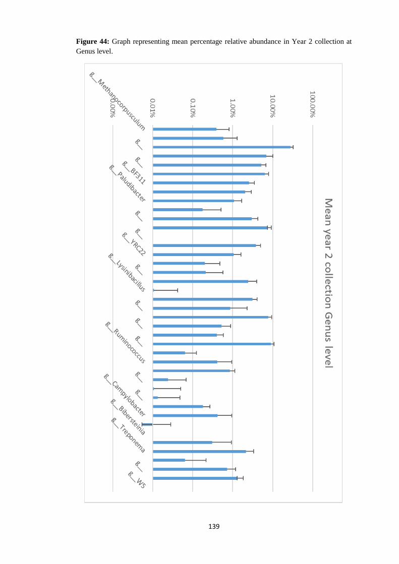
139


Genus level.

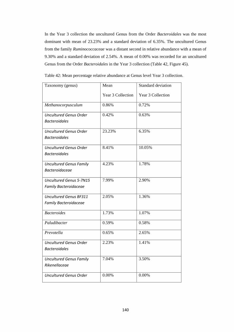
140

In the Year 3 collection the uncultured Genus from the Order Bacteroidales was the most

dominant with mean of 23.23% and a standard deviation of 6.35%. The uncultured Genus

from the family Ruminococcaceae was a distant second in relative abundance with a mean of

9.30% and a standard deviation of 2.54%. A mean of 0.00% was recorded for an uncultured

Genus from the Order Bacteroidales in the Year 3 collection (Table 42, Figure 45).



Year 3 Collection

Standard deviation

Year 3 Collection


Uncultured Genus Order

Bacteroidales

0.42% 0.63%


Bacteroidales

23.23% 6.35%


Bacteroidales

8.41% 10.05%

Uncultured Genus Family

Bacteroidaceae

4.23% 1.78%

Uncultured Genus 5-7N15


7.99% 2.90%



2.05% 1.36%





Bacteroidales

2.23% 1.41%


Rikenellaceae

7.04% 3.50%

Uncultured Genus Order 0.00% 0.00%

141

Bacteroidales

Uncultured Genus CF231


4.84% 2.14%



2.14% 1.86%



Bacteroidales

0.13% 0.55%




Clostridiales

2.76% 1.10%


Christendenellaceae

2.00% 7.20%



Lachnospiraceae

0.48% 0.63%

Uncultured Genus rc4-4


0.30% 0.26%


Ruminococcaceae

9.30% 2.54%





Erysipelotrichaceae

0.08% 0.49%

Uncultured Genus RFN20

Family Erysipelotrichaceae

0.05% 0.34%

Uncultured Genus Class

Alphaproteobacteria

0.08% 0.47%

142


Desulfovibrionaceae

0.19% 0.26%



Enterobacteriaceae

0.07% 0.25%


Uncultured Genus Phylum

Spirochaetes.

0.21% 0.39%



Verruco-5

0.09% 0.22%


Verruco-5

0.48% 0.46%


Unculture Genus W5 Family

Cloacamonaceae

0.05% 0.19%

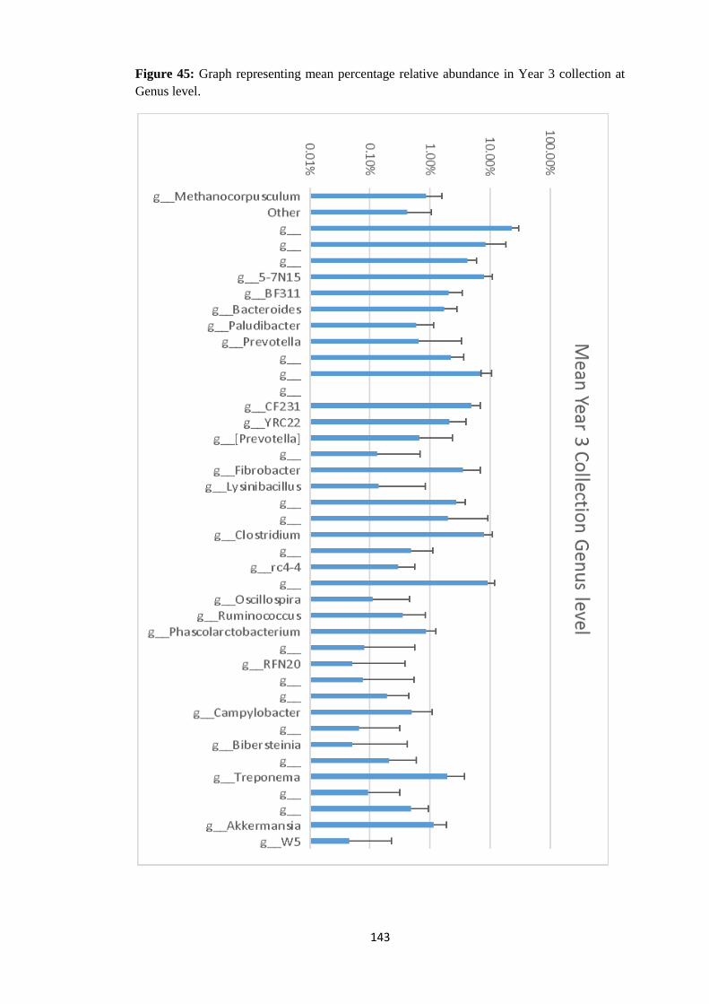
143


Genus level.

144

The uncultured Genus from the Order Bacteroidales had the highest mean percentage

relative abundance of 28.11% in the Year 2 collection. Another uncultured Genus from the

family Ruminococcaceae recorded a mean of 10.02% in the Year 1 collection. The Genus

Bibersteinia recorded a mean of 0.00% in both Year 1 and Year 2 collection and a mean of

0.05% in the Year 3 collection. Another uncultured Genus W5 from the family

Cloacamonaceae recorded a mean of 0.00% in both Year 1 and Year 2 collections while

recording a mean of 0.05% in the Year 3 collections (Table 43, Figure 46).

Table 43: Table comparing the mean percentage relative abundance in Year 1, Year 2 and

Year 3 collections Genus level of Taxonomy.


Year 1

Mean

Year 2

Mean

Year 3

Standard

deviation

Year 1

Standard

deviation

Year 2

Standard

deviation

Year 3

Methanocorpusculum 0.36% 0.39% 0.86% 0.34% 0.42% 0.72%

Uncultured Genus

Order Bacteroidales

0.31% 0.59% 0.42% 0.38% 0.71% 0.63%

Uncultured Genus

Order Bacteroidales

24.19% 28.11% 23.23% 4.57% 4.41% 6.35%

Uncultured Genus

Order Bacteroidales

3.60% 6.91% 8.41% 1.26% 3.19% 10.05%

Uncultured Genus


5.19% 5.19% 4.23% 1.41% 1.64% 1.78%

Uncultured Genus 5-

7N15,Family

Bacteroidaceae

7.96% 6.31% 7.99% 1.25% 1.59% 2.90%

Uncultured Genus

BF311 Family

Bacteroidaceae

2.34% 2.59% 2.05% 0.94% 0.92% 1.36%

Bacteroides 2.80% 2.07% 1.73% 1.23% 0.87% 1.07%

Paludibacter 0.64% 1.09% 0.59% 0.40% 0.61% 0.58%

Prevotella 1.13% 0.18% 0.65% 2.50% 0.33% 2.65%

Uncultured Genus,

Order Bacteroidales

2.80% 3.00% 2.23% 1.00% 1.32% 1.41%

145

Uncultured Genus


8.54% 7.43% 7.04% 2.27% 1.74% 3.50%

Uncultured Genus

Order Bacteroidales

0.16% 0.00% 0.00% 0.87% 0.00% 0.00%

Uncultured Genus

CF231 Family

Paraprevotellaceae

5.54% 3.82% 4.84% 1.45% 1.13% 2.14%

Uncultured Genus

YRC22 Family

Paraprevotellaceae

2.28% 1.05% 2.14% 1.36% 0.57% 1.86%

[Prevotella] 0.34% 0.20% 0.66% 0.38% 0.27% 1.68%

Uncultured Genus

Order Bacteroidales

0.11% 0.21% 0.13% 0.14% 0.36% 0.55%

Fibrobacter 2.28% 2.48% 3.52% 1.63% 1.55% 3.40%

Lysinibacillus 0.02% 0.01% 0.14% 0.04% 0.03% 0.70%

Uncultured Genus

Order Clostridiales

3.77% 3.12% 2.76% 1.37% 1.00% 1.10%

Uncultured Genus

Family

Christendenellaceae

0.41% 0.86% 2.00% 0.23% 1.43% 7.20%

Clostridium 8.92% 7.78% 8.01% 1.19% 1.63% 2.83%

Uncultured Genus

Family

Lachnospiraceae

0.58% 0.52% 0.48% 0.22% 0.38% 0.63%


4 Family

Peptococcaceae

0.33% 0.41% 0.30% 0.18% 0.18% 0.26%

Uncultured Genus

Family

Ruminococcaceae

10.02% 9.12% 9.30% 1.37% 1.58% 2.54%

Oscillospira 0.07% 0.06% 0.11% 0.08% 0.06% 0.35%

Ruminococcus 0.27% 0.41% 0.35% 0.23% 0.54% 0.49%

146

Phascolarctobacterium 0.79% 0.85% 0.85% 0.41% 0.30% 0.40%

Uncultured Genus

Family

Erysipelotrichaceae

0.04% 0.02% 0.08% 0.07% 0.04% 0.49%

Uncultured Genus

RFN20 Family

Erysipelotrichaceae

0.00% 0.01% 0.05% 0.00% 0.04% 0.34%

Uncultured Genus

Class

Alphaproteobacteria

0.00% 0.01% 0.08% 0.02% 0.03% 0.47%

Uncultured Genus

Family

Desulfovibrionaceae

0.18% 0.18% 0.19% 0.09% 0.09% 0.26%

Campylobacter 0.21% 0.42% 0.49% 0.35% 0.53% 0.59%

Uncultured Genus

Family

Enterobacteriaceae

0.01% 0.01% 0.07% 0.04% 0.02% 0.25%

Bibersteinia 0.00% 0.00% 0.05% 0.00% 0.00% 0.36%

Uncultured Genus


0.17% 0.31% 0.21% 0.22% 0.62% 0.39%

Treponema 1.73% 2.14% 1.95% 0.60% 1.18% 1.78%

Uncultured Genus

Class Verruco-5

0.02% 0.06% 0.09% 0.04% 0.15% 0.22%

Uncultured Genus

Class Verruco-5

0.70% 0.73% 0.48% 0.70% 0.47% 0.46%

Akkermansia 1.13% 1.29% 1.14% 0.56% 0.54% 0.74%

Unculture Genus W5,

Family

Cloacamonaceae

0.00% 0.00% 0.05% 0.00% 0.00% 0.19%

147

Figure 46: Graph comparing percentage mean relative abundance at Genus level in Year 1,

Year 2 sand Year 3 collections.

A plot of number of species as a function of number of samples was performed in the Year 1,

Year 2 and Year 3 collections. Species richness also known as alpha (α) diversity in all the

148

collection was determined by scaling down the number of sequences in all the samples to a

uniform or standardized sequence in all the samples and determining the number of species

in standardized samples.

Species richness is determined by the gradient of the rarefaction curve. A steep gradient is

indicative of higher species richness or a higher alpha diversity while a lower gradient is

indicative of a lower species richness or low alpha diversity. As can be seen in Figure 23,

year 1 collection (red curve) had a very slightly higher gradient than both the year 2

collection (blue curve) and year 3 collection (orange curve). What this means is that there are

slightly more species in year 1 collection than any of the other 2 collections. Looking closely

at the graph it will be observed that though year 1 collection (red curve) is slightly higher in

gradient it is very close to year 3 collection (orange curve). This means year 1 collection (red

curve) is very slightly higher in alpha diversity but is closely followed by year 3 collection

(orange curve).

Year 2 collection (blue curve) has the lowest gradient when compared to Year 1 and Year 3

collections. This means year 2 has slightly lowest alpha diversity. It should also be noted that

the gradients of the curves are not widely apart which suggest that the difference in species

richness amongst the collections is not markedly different. It can also be noted that the

gradient in Year 1 collection (red curve) and year 3 collection (orange curve) is much closer

than in Year 1 and Year 2 or in Year 3 and Year 2. This means that alpha diversity in Year 1

is much similar to Year 3 than Year 2 (Figure 47).

149

Figure 47: Rarefaction curve of year 1, year 2 and year 3 collections.

150

4.8.4 Shannon Diversity – Index Species richness and the proportion of distribution of each species in the Year 1, Year 2 and

Year 3 collection was measured and compared using Shannon diversity index.

Year 1 (red curve) collection has a slightly higher Shannon diversity index that the other 2

collections. This means that Year 1 (red curve) collection has a very slightly higher alpha

diversity with a more even distribution of species within the sample than the other 2

collections. The Shannon diversity also shows that year 2 collection has also a narrow higher

species richness with species more evenly distributed in the samples than in Year 3 (Figure

48).

151

Figure 48: Shannon diversity curve for the Year 1, Year 2 and Year 3 Collections.

152

4.8.5 Non – Metric Multidimensional Scaling. Similarity or resemblance between the samples in all the collection was measured and

compared using the Bray – Curtis statistical tool.

Samples were divided into Year 1 samples, Year 2 samples and Year 3 samples. There is a

clustering of samples based on resemblance or similarity. Samples that are not similar appear

wider apart on the 2 dimensional Bray – Curtis plot. The plot has a stress value of 0.1

revealing the fitness of the values into the 2 dimensional plot (Figure 49a).

153

Figure 49a: Bray – Curtis MDS plot base on relative abundance of OTUs for Year 1, Year 2

and Year 3 collections.

154

As can be seen from the MDS plot above (Figure 49a), there is a visual clustering of samples

in the Year 1, Year 2 and Year 3 collections. Samples in Year 1 collection (inverted blue

triangle), Year 2 collection (light blue square) and Year 3 (green triangle) cluster visually.

Samples in the Year 3 collections identified as BC1,BC36, BC35, BC39, BC45 appear as

outliers because of their lack of similarity to the other samples in the collections.

Employing PERMANOVA pair wise test to further analyses the data, a significant difference

in the clustering of Year 3 and Year 1 was observed with a P value of 0.001 and a t value of

2.119. PERMANOVA again showed a significant difference between the clustering of Year

3 and Year 2 with a P = 0.001 and t = 2.214. PERMANOVA pair wise test also revealed a

significant difference between the clustering of Year 1 and Year 2 collection with a P value

of 0.001 and a t value of 2.440.

PERMDISP pair wise test was also performed to further analyse the data. It revealed a

significant difference between Year 3 and Year 1 collections with P = 0.001 and t = 4.745. It

again showed a significant difference between Year 2 and Year 3 collections with P value of

0.001 and a t value of 4.453. However PERMDISP pair wise test revealed no significant

difference between Year 1 and Year 2 collections with P = 0.133 and t = 1.577.

To further analyse the collections another MDS plot was done without the outliers from the

Year 3 collections. The MDS plot had a 2D stress of 0.23 (Figure 49b). When the outliers

were removed a better appreciation of the visual difference in clustering was seen. With the

outliers removed, PERMANOVA pair wise test again revealed a significant difference in

clustering between Year 1 and Year 3 collections with a P value of 0.001 and a t value of

2.15. There was a significant difference in the clustering of Year 2 and Year 3 collections

with P = 0.001 and t = 2.287. Again PERMANOVA revealed significant difference in

clustering of Year 1 and Year 2 collection with P = 0.001 t = 2.440.

PERMDISP pair wise test also revealed significant difference in the clustering of Year 1 and

Year 3 collection with P = 0.001 and t = 5.917. There was a significant difference in Year 2

and Year 3 collection with a P value of 0.001 and a t value of 4.743. However PERMDISP

also showed no significant difference between Year 1 and Year 2 collections (Figure 49b).

155

Figure 49b : Bray – Curtis MDS plot base on relative abundance of OTUs for Year 1, Year

2 and Year 3 without outliers.

156

4.8.6 Statistical View of Outliers at Order level. From the MDS plot in figure 49a, BC1, BC36, BC35, BC39 and BC45 appear as outliers. All

the outliers are located in the Year 3 collection. It should also be noted that BC1 and BC36

are from the same animal identified as 810 and therefore act as biological replicates.

Percentage mean relative abundance for the Order Methanomicrobiales in the outliers was

0.54% with a standard deviation of 0.42%. Bacteroidales had a mean percentage relative

abundance of 58.20% with a standard deviation of 30.26%. Clostridiales had a mean of

30.84% and a standard deviation of 29.33%. Erysipelotrichales recorded a mean of 1.22%

while the Order Campylobacterales recorded a percentage mean of 1.02%. Bacillales had a

mean of 1.00%. Enterobacteriales had a mean of 0.06%. Pasteurellales recorded a mean of

0.54% while the order Spirochaetales had a mean of 1.90% with a standard deviation of

2.62%. Verrucomicrobiales had an average of 0.66%. the uncultured Order WCHB1-41from

the Class Verruco-5 had a mean of 0.88% and a standard deviation of 0.81% (Table 44,

Figure 50).

Table 44: Percentage mean relative abundance for the outliers (BC1,BC35,BC36,BC39 and

BC45) from the year 3 collection.

Taxonomy Mean of outliers at Order

level

Standard deviation of

Outliers







Unclassified Order

Class

Alphaproteobacteria

0.70% 1.57%



157



Uncultured Order

PL-11B10 Phylum

Spirochaetes

0.00% 0.00%


Uncultured

OrderWCHB1-41,

Class Verruco-5

0.88% 0.81%



158

Figure 50: Graph representing the average percentage relative abundance in the outliers

(BC1, BC35, BC36, BC39, BC45).

159

The order Methanomicrobiales recorded a mean percentage relative abundance of 0.54% in

the outliers and a mean of 0.36% and 0.39% in the Year 1 and Year 2 collections

respectively. The Order Bacillales recorded a percentage mean relative abundance of 1.00%

in the outliers, it however recorded a mean of 0.02% in the Year 1 collection and a mean of

0.01% in the Year 2 collection. Erysipelotriachales had a mean of 1.22% in the outliers,

0.06% in the Year 1 collection and 0.04% in the Year 2 collection. The Order

Campylobacterales recorded a mean of 1.02% relative abundance in the outliers, 0.21% in

the Year 1 collection and 0.42% in the Year 2 collection. Enterobacteriales had a percentage

mean relative abundance of 0.06% in the outliers and a mean of 0.01% in both the Year 1

and Year 2 collection. The Order Pasteurellales had a mean percentage relative abundance

of 0.54% in the outliers and 0.00% in both the Year 1 and Year 2 collections (Table 45,

Figure 51).

Table 45: Percentage mean relative abundance in the outliers, Year 1 collection, Year 2

collection and Year 3 collection minus the outliers at the Order level of Taxonomy.

Taxonomy Mean of

outliers at

order level

Mean order

level year 1

collection

Mean year

2

collection

Mean

year 3

collection

minus

outliers


Bacteroidales 58.20% 67.94% 68.75% 67.17%


Bacillales 1.00% 0.02% 0.01% 0.05%

Clostridiales 30.84% 25.17% 23.15% 23.49%

Erysipelotrichales 1.22% 0.06% 0.04% 0.02%

Unclassified Order

Class

Alphaproteobacteria

0.70% 0.00% 0.01% 0.01%



Enterobacteriales 0.06% 0.01% 0.01% 0.07%

Pasteurellales 0.54% 0.00% 0.00% 0.00%

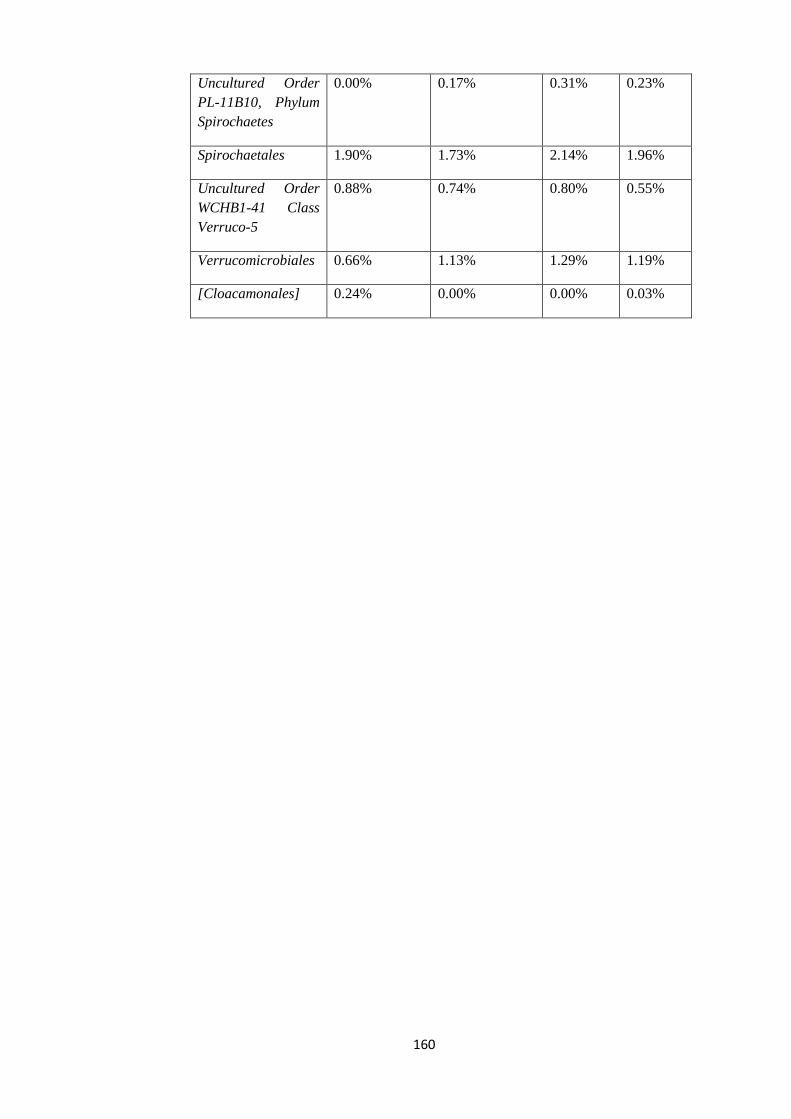
160

Uncultured Order

PL-11B10, Phylum

Spirochaetes

0.00% 0.17% 0.31% 0.23%

Spirochaetales 1.90% 1.73% 2.14% 1.96%

Uncultured Order

WCHB1-41 Class

Verruco-5

0.88% 0.74% 0.80% 0.55%


[Cloacamonales] 0.24% 0.00% 0.00% 0.03%

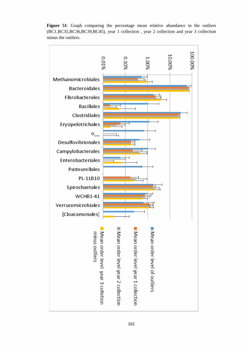
161

Figure 51: Graph comparing the percentage mean relative abundance in the outliers

(BC1,BC35,BC36,BC39,BC45), year 1 collection , year 2 collection and year 3 collection

minus the outliers.

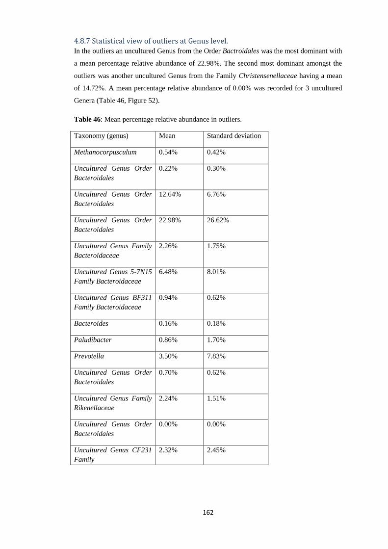
162

4.8.7 Statistical view of outliers at Genus level. In the outliers an uncultured Genus from the Order Bactroidales was the most dominant with

a mean percentage relative abundance of 22.98%. The second most dominant amongst the

outliers was another uncultured Genus from the Family Christensenellaceae having a mean

of 14.72%. A mean percentage relative abundance of 0.00% was recorded for 3 uncultured

Genera (Table 46, Figure 52).

Table 46: Mean percentage relative abundance in outliers.

Taxonomy (genus) Mean Standard deviation



Bacteroidales

0.22% 0.30%


Bacteroidales

12.64% 6.76%


Bacteroidales

22.98% 26.62%


Bacteroidaceae

2.26% 1.75%

Uncultured Genus 5-7N15


6.48% 8.01%



0.94% 0.62%





Bacteroidales

0.70% 0.62%


Rikenellaceae

2.24% 1.51%


Bacteroidales

0.00% 0.00%

Uncultured Genus CF231

Family

2.32% 2.45%

163

Paraprevotellaceae


Family

Paraprevotellaceae

0.78% 1.01%



Bacteroidales

0.00% 0.00%




Clostridiales

2.16% 2.03%


Christendenellaceae

14.72% 21.73%



Lachnospiraceae

1.08% 2.03%

Uncultured Genus rc4-4


0.42% 0.77%


Ruminococcaceae

6.30% 2.47%





Erysipelotrichaceae

0.72% 1.61%

Uncultured Genus RFN20

Family

Erysipelotrichaceae

0.50% 1.12%


Alphaproteobacteria

0.70% 1.57%


Desulfovibrionaceae

0.42% 0.83%

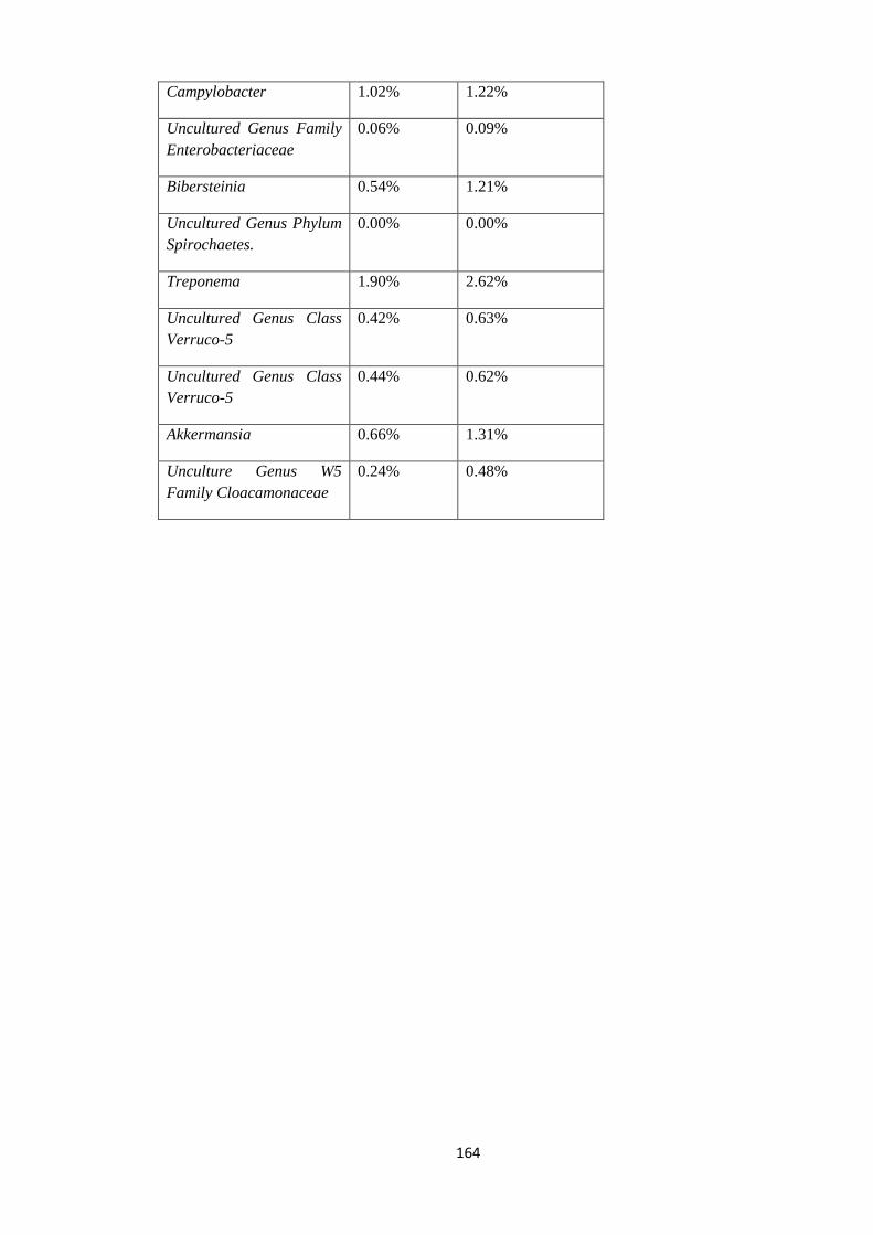
164



Enterobacteriaceae

0.06% 0.09%


Uncultured Genus Phylum

Spirochaetes.

0.00% 0.00%



Verruco-5

0.42% 0.63%


Verruco-5

0.44% 0.62%


Unculture Genus W5

Family Cloacamonaceae

0.24% 0.48%

165

Figure 52: Graph showing mean percentage relative abundance Genus level in outliers.

166

The uncultured Genus from the Order Bacteroidales recorded its most dominant mean

percentage relative abundance of 28.11% in the Year 2 collection. It recorded a mean of

12.64% in the outliers which are originally all members of the year 3 collections. Another

uncultured Genus from the Order Bacteroidales had a mean percentage relative of 22.98% in

the outliers. The Genus Bibersteinia had a mean percentage relative abundance of 0.54% in

the outliers but recorded a mean of 0.00% in all the other collections. The Genus

Lysinbacillus had mean of 1.00% in the outliers which exceeds its relative abundance in the

other collections. The Genus Oscillospira was most dominant in the outliers with mean of

0.56% (Table 47, Figure 53).

Table 47: Table comparing mean percentage relative abundance in Year 1, Year 2, Year 3

minus outliers, and outliers.

Taxonomy (Genus) Mean

Year

1

Mean

year

2

Mean

Year

3

witho

ut

outlie

rs

Mean

outlie

rs

only

Standa

rd

deviati

on

Year 1

Standa

rd

deviati

on

year 2

Standa

rd

deviati

on

outlier

s only

Standa

rd

deviati

on year

3

collecti

on

withou

t

outliers

Methanocorpusculu

m

0.36

%

0.39

%

0.89

%

0.54

%

0.34% 0.42% 0.42% 0.73%

Uncultured Genus

Order Bacteroidales

0.31

%

0.59

%

0.44

%

0.22

%

0.38% 0.71% 0.30% 0.66%

Uncultured Genus

Order Bacteroidales

24.19

%

28.11

%

24.29

%

12.64

%

4.57% 4.41% 6.76% 5.30%

Uncultured Genus

Order Bacteroidales

3.60

%

6.91

%

6.95

%

22.98

%

1.26% 3.19% 26.62

%

5.44%

Uncultured Genus

Family

Bacteroidaceae

5.19

%

5.19

%

4.43

%

2.26

%

1.41% 1.64% 1.75% 1.67%

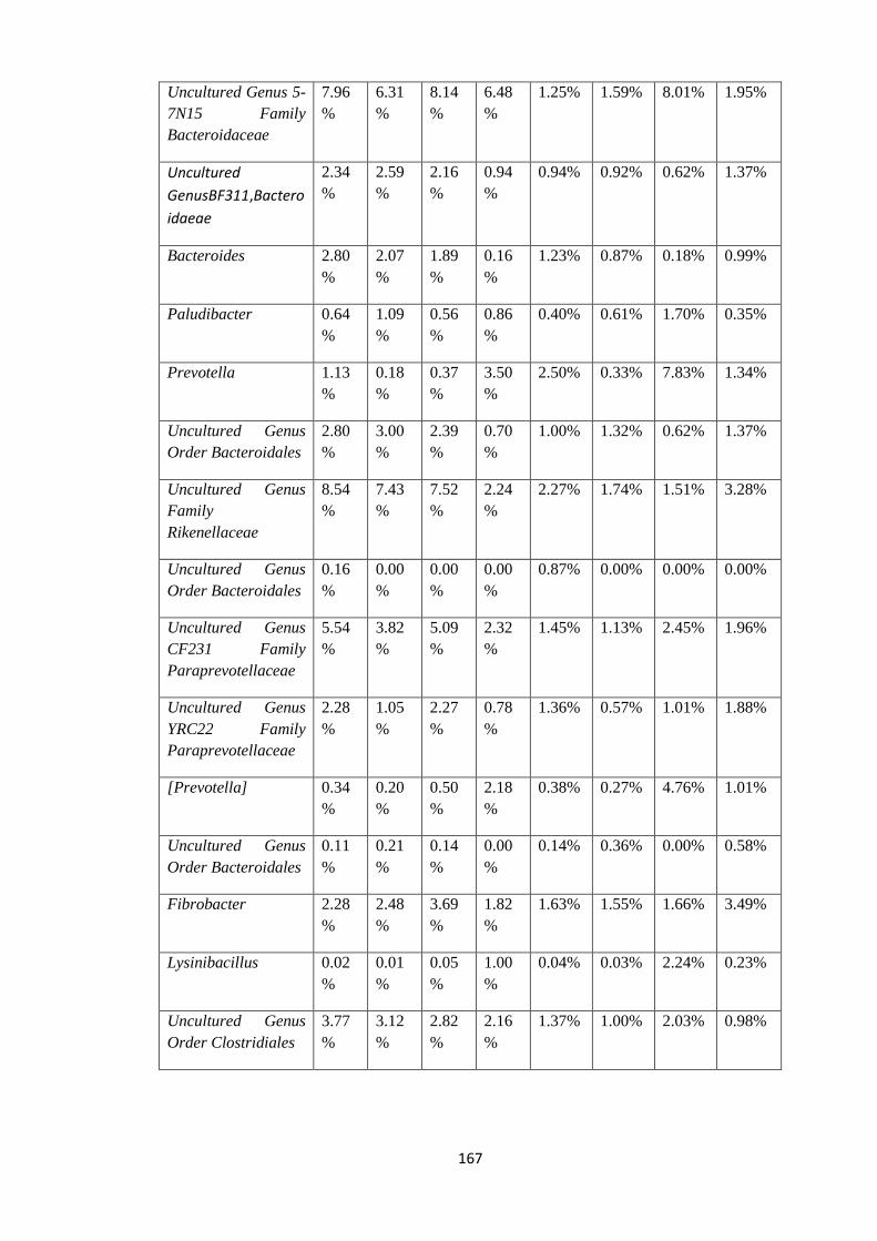
167

Uncultured Genus 5-

7N15 Family

Bacteroidaceae

7.96

%

6.31

%

8.14

%

6.48

%

1.25% 1.59% 8.01% 1.95%

Uncultured

GenusBF311,Bactero

idaeae

2.34

%

2.59

%

2.16

%

0.94

%

0.94% 0.92% 0.62% 1.37%

Bacteroides 2.80

%

2.07

%

1.89

%

0.16

%

1.23% 0.87% 0.18% 0.99%

Paludibacter 0.64

%

1.09

%

0.56

%

0.86

%

0.40% 0.61% 1.70% 0.35%

Prevotella 1.13

%

0.18

%

0.37

%

3.50

%

2.50% 0.33% 7.83% 1.34%

Uncultured Genus

Order Bacteroidales

2.80

%

3.00

%

2.39

%

0.70

%

1.00% 1.32% 0.62% 1.37%

Uncultured Genus

Family

Rikenellaceae

8.54

%

7.43

%

7.52

%

2.24

%

2.27% 1.74% 1.51% 3.28%

Uncultured Genus

Order Bacteroidales

0.16

%

0.00

%

0.00

%

0.00

%

0.87% 0.00% 0.00% 0.00%

Uncultured Genus

CF231 Family

Paraprevotellaceae

5.54

%

3.82

%

5.09

%

2.32

%

1.45% 1.13% 2.45% 1.96%

Uncultured Genus

YRC22 Family

Paraprevotellaceae

2.28

%

1.05

%

2.27

%

0.78

%

1.36% 0.57% 1.01% 1.88%

[Prevotella] 0.34

%

0.20

%

0.50

%

2.18

%

0.38% 0.27% 4.76% 1.01%

Uncultured Genus

Order Bacteroidales

0.11

%

0.21

%

0.14

%

0.00

%

0.14% 0.36% 0.00% 0.58%

Fibrobacter 2.28

%

2.48

%

3.69

%

1.82

%

1.63% 1.55% 1.66% 3.49%

Lysinibacillus 0.02

%

0.01

%

0.05

%

1.00

%

0.04% 0.03% 2.24% 0.23%

Uncultured Genus

Order Clostridiales

3.77

%

3.12

%

2.82

%

2.16

%

1.37% 1.00% 2.03% 0.98%

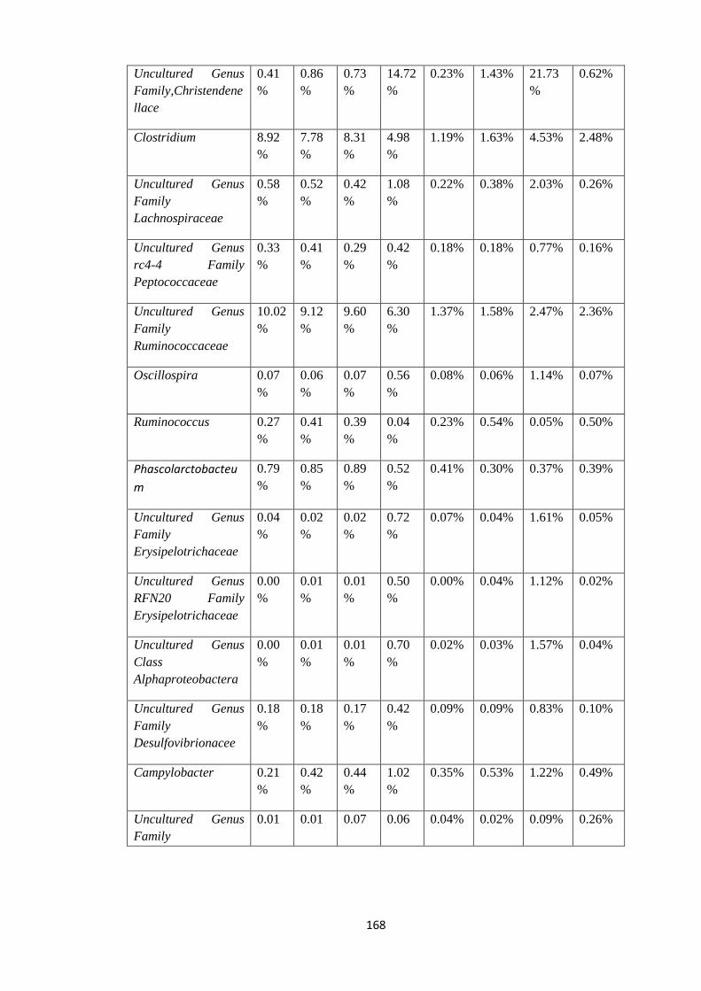
168

Uncultured Genus

Family,Christendene

llace

0.41

%

0.86

%

0.73

%

14.72

%

0.23% 1.43% 21.73

%

0.62%

Clostridium 8.92

%

7.78

%

8.31

%

4.98

%

1.19% 1.63% 4.53% 2.48%

Uncultured Genus

Family

Lachnospiraceae

0.58

%

0.52

%

0.42

%

1.08

%

0.22% 0.38% 2.03% 0.26%

Uncultured Genus

rc4-4 Family

Peptococcaceae

0.33

%

0.41

%

0.29

%

0.42

%

0.18% 0.18% 0.77% 0.16%

Uncultured Genus

Family

Ruminococcaceae

10.02

%

9.12

%

9.60

%

6.30

%

1.37% 1.58% 2.47% 2.36%

Oscillospira 0.07

%

0.06

%

0.07

%

0.56

%

0.08% 0.06% 1.14% 0.07%

Ruminococcus 0.27

%

0.41

%

0.39

%

0.04

%

0.23% 0.54% 0.05% 0.50%

Phascolarctobacteu

m

0.79

%

0.85

%

0.89

%

0.52

%

0.41% 0.30% 0.37% 0.39%

Uncultured Genus

Family

Erysipelotrichaceae

0.04

%

0.02

%

0.02

%

0.72

%

0.07% 0.04% 1.61% 0.05%

Uncultured Genus

RFN20 Family

Erysipelotrichaceae

0.00

%

0.01

%

0.01

%

0.50

%

0.00% 0.04% 1.12% 0.02%

Uncultured Genus

Class

Alphaproteobactera

0.00

%

0.01

%

0.01

%

0.70

%

0.02% 0.03% 1.57% 0.04%

Uncultured Genus

Family

Desulfovibrionacee

0.18

%

0.18

%

0.17

%

0.42

%

0.09% 0.09% 0.83% 0.10%

Campylobacter 0.21

%

0.42

%

0.44

%

1.02

%

0.35% 0.53% 1.22% 0.49%

Uncultured Genus

Family

0.01 0.01 0.07 0.06 0.04% 0.02% 0.09% 0.26%

169

Enterobacteriacee % % % %

Bibersteinia 0.00

%

0.00

%

0.00

%

0.54

%

0.00% 0.00% 1.21% 0.01%

Uncultured Genus

Phylum

Spirochaetes.

0.17

%

0.31

%

0.23

%

0.00

%

0.22% 0.62% 0.00% 0.40%

Treponema 1.73 2.14 1.96 1.90 0.60% 1.18% 2.62% 1.72%

Uncultured Genus

Class Verruco-5

0.02

%

0.06

%

0.06

%

0.42

%

0.04% 0.15% 0.63% 0.09%

Uncultured Genus

Class Verruco-5

0.70

%

0.73

%

0.49

%

0.44

%

0.70% 0.47% 0.62% 0.45%

Akkermansia 1.13

%

1.29

%

1.19

%

0.66

%

0.56% 0.54% 1.31% 0.66%

Unculture Genus W5

Family

Cloacamonaceae

0.00

%

0.00

%

0.03

%

0.24

%

0.00% 0.00% 0.48% 0.12%

170

Figure 53: Graph comparing mean percentage relative abundance in Year1, Year2, Year 3

without outliers, and outliers.

171

172

4.9 MDS plot for Study 1 and Study 2. In an attempt to have an overview of the 2 studies namely:

Study 1: Helminth only infected sheep study.

Study 2: MAP and helminth infected sheep study using only the Year 3 collection.

An MDS plot was carried out to give a broader picture on the gastrointestinal microbiome in

the 2 studies.

173

Figure 54: MDS plot of Study 1 (Helminth only infected sheep) and Study 2 (MAP and

helminths infected sheep).

174

PERMANOVA pair – wise test showed a significant difference in the clustering between

Study 1 and Study 2 with a P value of 0.001 and a t value of 3.685. PERMANOVA main test

also revealed a significant difference in study 1 and study 2 with a P value of 0.001 and a

Pseudo F value of 13.581. PERMDISP pair wise comparison did not show significant

difference with a P value of 0.758 and t = 0.319.

175

5. DISCUSSION In the first part of this study, the gastrointestinal microbiomes of different sheep groups

were analysed to understand the effect of helminthiasis on the gut microbiome of sheep

that are not infected with Mycobacterium avium subspecies paratuberculosis (MAP).

Illumina MiSeq platform was use to carryout analysis of the V4 region of the 16SrRNA gene.

Quantitative Insight Into Microbial Ecology (QIIME) was used to further investigate the raw

sequences data obtained from Edinburgh Genomics for Operational Taxonomic Unit (OTU)

picking, Taxonomic assignment, alpha diversity analysis and beta diversity analysis. Non

metric multidimensional plots were use to determine relationships between Operational

taxonomy units based on similarity. PRIMER and PERMANOVA statistical tools were

employed to investigate further the level significant difference between samples.

In the second part of the study, the gastrointestinal microbiome of sheep infected with

MAP and helminths were examined and analysed. Illumina MiSeq sequencing was used to

examine the V4 region of the prokaryotic 16SrRNA gene. QIIME was used to investigate the

raw data obtained from Edinburgh genomics. MDS plots using Bray-Curtis similarity curve

were plotted to determine the relationship between OTUs based on resemblance.

Statistically analysis were carried out by the PRIMER and PERMANOVA tools.

The two studies were then compared to analyse whether there was a difference in the

microbiomes of sheep dually infected with both JD and gastrointestinal roundworms and

those only infected with the roundworms. MDS plots were plotted and statistical tools

PERMANOVA and PERMDISP were used to analyse significance in difference between the 2

studies.

5.1 Gastrointestinal Microbiome the main objective of this study is to discover the effect of intestinal infections on the

gastrointestinal microbiome of sheep focussing on helminthiasis and Johne’s disease of

sheep. In Helminth infected group, which is the first part of the study, 38 pre-treatment

amplicons and 37 post-treated amplicons were examined by analysing the V4 region of the

16SrRNA gene using Illumina MiSeq platform.

In the MAP infected group which is the second part of the study the V4 region of the

16SrRNA of 29 amplicons from the Year 1 collection, 40 amplicons from Year 2 collection

176

and 56 amplicons from Year 3 collections were analysed by the use of Illumina MiSeq

platform.

5.2 Helminth infected group Sheep in this group were positive for helminthiasis. The V4 region of the 16SrRNA of 38 pre-

treatments and 37 post treated amplicons were analysed by Illumina MiSeq platform.

QIIME pipeline was use to analyse the raw data obtained. In all the samples in this group

(Pre-treatment plus post-treated) QIIME revealed the Phylum Bacteroidetes as the most

dominant followed by Firmicutes (Henderson et al., 2015). Other Phyla observed amongst

the 8 top in the helminth infected group include Fibrobacteres, Proteobacteria,

Spirochaetes, Tenerictutes and Verrucomicrobia.

The Phylum Bacteroidetes was slightly higher in the post-treated samples (59.26%) than the

pre-treatment samples (58.26%), Fibrobacteres was also slightly higher in the post-treated

(5.25%) than the pre-treatment samples (4.65%). Firmicutes was slightly higher in the pre-

treatment samples than the post-treated samples while Tenericutes was higher in post-

treated samples than pre-treatment sample. These marginal variations of change in relative

abundance at the Phylum level might suggest that the administration of anthelminthic does

not drastically change the microbiome in any particular pattern at the Phylum level.

At the Order level of taxonomy, the Order Bacteroidales was slightly higher in the post-

treated samples (59.26%) than the pre-treatment samples (58.26%). The same pattern was

also seen in the Fibrobacterales with post- treated samples recording a mean of 5.25% and

pre-treatment samples having a mean of 4.65%. the Order Clostridiales was only marginally

higher in pre-treatment (29.05%) than in post-treated samples (27.99%). The uncultured

Deltaproteobacterium GMD14H09 was more dominant in the pre-treatment samples

(0.24%) than the post-treated samples (0.08%). The opposite is true for another uncultured

Order RF39 which was less dominant in the pre-treatment samples (0.04%) than the post-

treated samples (0.12%). Again These variations in percentage relative abundance do not

show an obvious pattern in the effect of the anthelminthic on the gut microbiome at the

Order level of Taxonomy which might suggest that the anthelminthic drug does not show

any effect on the gut microbiome at the Order level of Taxonomy.

At the Genus level the uncultured Genus from the Order Bacteroidales was marginally

higher in the post treated samples (23.73%) than the pre-treatment (20.85%). In both pre-

177

treatment and post-treated samples another uncultured Genus from the Family

Ruminococcaceae was next in relative abundance with its mean slightly higher in post-

treated (9.86%) than pre-treatment samples (9.60%). The uncultured Genus from the

uncultured Order RF39 from the Class Mollicutes was the least dominant in the pre-

treatment samples (0.04%) while the least dominant in the post-treated sample was

another uncultured Genus from an uncultured Order GMD14H09 from the Class Mollicutes

(0.08%). Most of the Genera show only slight differences between the pre-treatment and

post treated samples in no particular pattern, therefore it can be suggested that even at the

Genus level there was no clear distinction between the relative abundance in the pre-

treatment and post-treated samples which might suggest that the anthelminthic used is not

causing any change in the gut microbiome.

In The post-treated groups (1, 2 and 3) an uncultured Genus from the Order Bacteroidales

was most dominant followed by another uncultured Genus from the Family

Ruminococcaceae which was closely followed by the Genus Clostridium in all the 3 groups

except in group 2 where the Genus Fibrobacter (7.21%) was slightly higher than the Genus

Clostridium (6.21%).

5.2.1 Pre- treatment and Post – treated groups based on anthelminthic.

The similarity between pre-treatment samples and the different groups of the post treated

samples were measured by Bray – Curtis similarity plots. PERMDISP pairwise comparison

showed no significant difference observed in the clustering of pre – treatment samples and

group 2 (Startect®) with P = 0.265 and t = 1.489. It also showed no significant difference in

the pre – treatment and group 3 (Zolvix®), + Startect®) with P value of 0.193 t value of

1.692. PERMDISP revealed a marginal significant difference in the clustering of pre –

treatment and group 1 (Zolvix®) with a P = 0.022 and t = 2.621. There was no significance

difference in the clustering of group 2 (Startect®) and group 3 (Zolvix® + Startect®) with

P = 0.689 and t = 0.440. There was also no significance difference in the clustering of group

1 (Zolvix®) and group 2 (Startect®) with a P value of 0.287 and a t value of 1.225.

PERMDISP pairwise comparison also showed no significant difference in the clustering of

the group 1 (Zolvix®) and group 3 (Zolvix®), + Startec®) with P = 0.436 t = 0.917. This

suggest that the overall PERMDISP clustering of the different groups from the centroid

178

when the different groups were paired was not significantly different with P = 0.062 and an

F value of 3.583.

PERMANOVA pair wise test showed there was no significant difference between the

clustering of the pre-treatment samples and the clustering of group 2 (Startect®) with P =

0.166 and a t value of 1.0841. PERMANOVA revealed a marginal significant difference

between the clustering of pre-treatment samples and the group 3 (Zolvix®) + Startect®)

with P = 0.052 and t value of 1.159. It also showed no significant difference when the pre-

treatment samples were paired with group 1 (Zolvix®)) with P = 0.06 and t = 1.156. When

PERMANOVA paired group 2 (Startect®) and group 3 (Zolvix® + Startect®), it also

revealed no significant difference in the clustering with p value of 0.206 and t value of

1.0535. There was also no significant difference in the clustering of group 1 (Zolvix®) and

group 2 (Startect®) with P = 0.161 and t = 1.059. PERMANOVA revealed a significant

difference in clustering of group 3 (Zolvix® + Startect®) and group 1 (Zolvix) with a P

value of 0.01 and t value of 1.169.

It can be observed from the PERMANOVA pair wise test that a significant difference is seen

when the when group 3 (Zolvix® + Startect®) is paired with group 1 (Zolvix®) with P

value of 0.01 and also when group 3 (Zolvix® + Startect®) is paired with the pre-

treatment with P value of 0.052. this might be as a result of the combined effect of the 2

anthelminthic they related with microbiome. But again this can be mere speculation

because the same pattern of difference was not seen when group 3 (Zolvix® + Startect®)

is paired with group 2 (Startect®) with P value of 0.206.

Comparing the pre – treatment samples with the different post treatment groups at the

Order level revealed that the Order Bacteroidales was higher in group 3 (63.13%) than

group 1 (57.25%) and group 2 (58.56%) and pre-treatment (58.26%). The Order

Fibrobacterales was lowest in group 3 (2.28%) and highest in group 2 (7.12%), and recorded

a mean of 5.73% and a mean of 4.65% in groups 1 and pre-treatment samples respectively.

An uncultured Order GMD14H09 was slightly lower in group 3 (0.06%) than other groups.

The same also applies for another uncultured Genus RF39 with a mean of 0.01% in group 3.

179

Some marginal variations have been observed between the group 3 samples and the other

groups, but it is still inconclusive to say that the changes in the microbiome were due to the

combination of the 2 anthelminthic drug Zolvix® and Startect®.

At the Genus level, the uncultured Genus from the Order Bacteroidales was slightly higher

in group 3 (26.07%) than in the pre-treatment (20.85%), group 1 (22.86%), group 2

(22.87%). The Genus Fibrobacter had the least dominance in group 3 (2.28%) and most

dominance in group 2 (7.12%). The Genus Ruminococcus had the least dominance also in

group 3 (0.08%) with highest dominance of 0.35% in group 1. An uncultured Genus from

the Class Mollicutes also recorded the least dominance in group 3 (0.01%) than in pre –

treatment (0.04%), group 1 (0.25%) and group 2 (0.01%).

Another uncultured Genus from the Order Bacteroidales was also least dominant in group 3

(0.03%) than in all the other groups.

At the Genus level, some degree of variations was observed in all the groups. Some Genera

were more abundant in one group and less abundant in another. This does not show any

particular pattern so it will be inconclusive to say whether it was the effect of the

anthelminthic or not.

A trend that was also observed in the MDS plot is that the outliers appear predominantly in

the pre-treatment group which seems to go back into the centre after treatment amongst

the post treated group, this is just a trend that might suggest an alteration of the gut

microbiome of the outliers after treatment making them more similar to the others.

5.2.2 Pre – treatment outliers compared to group 1, group2 and group 3.

The pre – treatment outliers observed in the MDS plots were analysed on the basis of

relative abundance at the Genus level of Taxonomy. The Genus Methanocorpusculum was

most dominant in the outliers (2.07%) than in group 1 (0.63%), group 2 (1.42%) and group 3

(1.15%). An unknown Genus from the Order Bacteroidales was also least dominant in the

outliers (15.67%) than the group 1 (22.86%), group 2 (22.87) and group 3 (26.07%). An

uncultured Genus from the Order Bacteroidales had a mean of 10.43% in the outliers which

was the highest as compared to group 1 (4.53%), group 2 (6.16%) and group 3 (6.46%).

Another uncultured Genus 5-7N15 from the Family Bacteroidaceae recorded the highest

mean of 11.13% in the outliers. The Genus Prevotella had a mean of 0.00% only in the

outliers. Interestingly, the outliers had the highest mean of 5.79% for the Genus

180

Campylobacter which recorded a mean of 1.17% in group 1, 1.57% in group 2 and 1.22% in

group 3.

These variations seen in the relative abundance of the Outliers observed at the Genus level

could be attributed to the fact that sheep (gimmers) were sourced from different locations

living under different conditions, exposed to different types of diseases and parasites , fed

different kinds of diet, administered different kinds of medication (Carding et al., 2015) .

The period of quarantine might also not have been adequate for the gut microbiome to

adjust as to reflect some degree of uniformity with all the other gimmers.

5.3 MAP and round worm dual infected group (Year 1 collection, Year 2

and Year 3 collection. Sheep in this group had dual infection with MAP and helminths. Rectal faecal samples were

collected annually for a period of 3 years identified as Year 1 collection, Year 2 collection

and Year 3 collections. Year 1 collection had 29 samples that were extracted, PCR generated

by Jelena Nikolić (previous student), in 2014. Year 2 collection had 40 samples that were

extracted and PCR generated by Miriam Navarro (previous student). Year 3 collection had

56 samples that were extracted and their PCR generated during this project. All the

amplicons in all the collections were sequenced using the Illumina MiSeq platform. QIIME

pipeline was used to analyse the raw data obtained from Edinburgh Genomics. QIIME

revealed the Phylum Bacteroidetes as the most dominant (67.5%) followed by the Phylum

Firmicutes (24.3%). Other Phyla include Euryarchaeota, Fibrobacteres, Proteobacteria,

Spirochaetes, Verrucomicrobia and an uncultured Phylum WWE1.

PERMANOVA pair-wise test revealed a significant difference in clustering between the Year

3 collection and the Year 1 collection with a P = 0.001 and t = 2.119. There was also a

significant difference in clustering observed by PERMANOVA between the Year 3 collection

and the Year 2 collection with a P value of 0.001 t value of 2.214. Again PERMANOVA

showed a significant level of difference between the Year 1 collection and the Year 2

collection with P = 0.001 and t = 2.440. These significant differences observed in the

different pair-wise PERMANOVA might be attributed to the changes in the gut microbiome

as result of the effects or clinical signs associated with MAP infection and or helminths

infection which might alter the gut microbiome. PERMANOVA also revealed that average

similarity within Year 1 collection was higher (65.14) than the average similarity within Year

2 (63.276) and within Year 3 (51.488). These might suggest that as the disease condition

181

progresses there was the likelihood of variations occurring in the gut microbiome.

PERMDISP pair wise comparisons revealed a significant difference in the clustering between

Year 1 and Year 3 collections with a P value of 0.001 and a t value of 4.745. There was also a

significant difference in the clustering between Year 2 and Year 3 collection P = 0.001 and t

= 4.453. PERMDISP however did not show a significant difference between Year 1 and Year

2 collection with P value of 0.133 and t value of 1.577. Again it can be argued here that the

progression of the disease might have played a role in detecting the degree of significant

difference in the clustering between the collections.

At the Order level of taxonomy, the Order Methanomicrobiales had the highest mean

percentage relative abundance in Year 3 which stood at 0.86% as compared to Year 1

(0.36%) and Year 2 (0.39%). Also another Order Bacialles had the highest mean in Year 3

collection (0.14%) as compared to Year 1 (0.02%) and Year 2 (0.01%). The Order

Erysipelotrichales again recorded the highest mean in Year 3 at 0.13% when compared to

Year 1 (0.06%) and Year 2 (0.04%). Enterobacteriales was higher in Year 3 (0.08%) than

Years 1 and 2 were both (0.01%). The Order Pasteurella was only present in Year 3 with a

mean of 0.05%. The Order Cloacamonales was only present in Year 3 with a mean of 0.05%

as well. At the Order level of taxonomy, it can be seen that Year 3 collection recorded

higher mean of relative abundance in quite a number of Orders than what was observed in

Year 1 and Year 2. Also Year 3 collection had some Orders (Pasteurella, Cloacamonales and

an uncultured Order from the Class Alphaproteobacteria) which were not present in Year 1

and Year 2 collections. Year 3 collection had varied from both Year 1 and Year 2 at the

Order level of Taxonomy which might be due to disease conditions or other factors

affecting the gut microbiome such as undiagnosed diseases and parasitic infections, diet,

toxins (Carding et al., 2015).

At the Genus level of Taxonomy Methanocorpusculum had its highest mean in the Year 3

collection at 0.86% when compared to 0.36% in Year 1 and 0.39% in Year 2. Another Genus

Lysinbacillus also had the highest mean in Year 3 (0.14%) than Year 1 (0.02%) with its lowest

recorded in Year 2 (0.01%). The Genus Bibersteinia was only seen in the Year 3 collection

with a mean of 0.05%. An unknown Genus W5 from the Family Cloacamonaceae was also

only observed in the Year 3 collection at a mean of 0.05%. A lot of uncultured bacteria at

the Genus level were observed making it difficult to say whether variations at this stage can

182

be clearly seen, but from the Genera observed the Year 3 collection might be showing some

degree of variations from Year 1 and Year 2 collections.

5.3.1 Year 3 collection outliers compared to Year 1 and Year 2.

Year 3 outliers observed in the MDS plots were examined based on average relative

abundance of the Genera found in them. An uncultured Genus from the Order

Bacteroidales recorded a mean of 22.98% in the outliers which was about seven times that

recorded in the Year 1 collection (3.60%) and three times what was recorded in Year 2

collection (6.91%). The Genus Bacteroides had a mean of 0.16% in the outliers, which was

lower that what was recorded in the Year 1 (2.80%) and Year 2 (2.07%). The Genus

Prevotella was highest in the outliers with a mean of 3.50%. An uncultured Genus from the

Family Rikenellaceae recorded a mean of 2.24% in the outliers which was lower that what

was recorded in Year 1 (8.54%), Year 2 (7.43%). The Genus Lysinbacillus had a mean of

1.00% in the outliers, 0.02% in Year 1 and 0.01% in the Year 2 collection. Another

uncultured Genus from the Family Christenesenellaceae recorded a mean of 14.72% in the

outliers which exceeded what it recorded in the Year 1 (0.41%) and Year 2 (0.86%)

collections. The Genus Campylobacter had a mean of 1.02% in the outliers, it had a mean of

0.21% and 0.42% in the Year 1 and Year 2 collections respectively. Another variation worthy

of note in the outliers is that the Genus Bibersteinia and another uncultured Genus W5

from the Family Cloacamonaceae were only present in the outliers and not in the Year 1 or

Year 2 collections at a mean of 0.54% for Bibersteinia and 0.24% for the uncultured Genus

W5 respectively.

One of the outliers tested positive by nested real time PCR of IS900 gene (result kindly

provided by Dr Celia Leao). Another outlier tested positive for serum antibody. Two of the

outliers tested negative to serum antibody test.

It can be suggested that as Johne’s disease progresses in sheep, it can cause changes in the

gut microbiome with the gut microbiome becoming more different in sick animals when

compared to healthy ones. More work is required in order to substantiate that the changes

in the gut microbiome are due specifically to Johne’s disease and not the consequence of

other diseases or conditions within the flock. Although the sheep sampled were from a

closed flock, limiting the numbers of sheep being introduced to the farm, it is possible that

new diseases could have been introduced by new animals being introduced or co-grazing

with other flocks or cattle or wildlife. A vaccination study is currently underway, to

183

vaccinate sheep against Johne’s disease, to compare the vaccinated sheep with those sheep

that were not vaccinated within the same flock so as to reduce the spread of the disease

and to further determine whether the microbiome of the vaccinated sheep differ from the

microbiome of the unvaccinated sheep.

5.4 Overall comparison of study 1 and study 2. The gastrointestinal microbiome of sheep in study 1 and the gastrointestinal microbiome of

sheep in study 2 were compared by plotting an MDS curve. PERMANOVA pair wise test

revealed a significant difference between study 1 and study 2 with a P value of 0.001 and t

value of 3.685. This difference in the gut microbiome might be as a result of diet, location,

drugs, toxins and pathogens that the sheep in the 2 different studies were exposed to

(Carding et al., 2015). On the other hand, PERMDISP showed no significant difference

between the clustering of Study 1 samples and Study 2 samples with a P value of 0.758 and

a t value of 0.319. This might suggest that there is more happening in the sheep which

might be as result of exposure to pathogens, diet or other factors in the wider environment

that is causing some form of resemblance in the gut microbiome.

184

6. Conclusion. In study 1 the effect of helminth infection and anthelminthic treatment on the

gastrointestinal microbiome was examined and analysed. The pre-treatment samples on

comparison with the 3 groups of post treated samples showed no significant difference in

the gastrointestinal microbiome with P>0.05. This study revealed that there are variations

in relative abundance at different level of taxonomy observed in the pre-treatment and the

different groups of the post-treated samples. It is still immature to say that this differences

were as a result of the effect of the anthelminthic used. A more precise experimental

design involving animals of the same age and breed, raised from the same environmental

conditions and fed the same kind of diet should be organised and carried out so as to

obtain more reliable results and outcomes.

In study 2 involving the dually MAP and helminth infected sheep it was discovered that

variations in the gastrointestinal microbiome occured as disease progress in sheep with

Year 3 sheep showing significant difference from the Year 1 and Year 2 sheep with P =

0.001. This might suggest that as Johne’s disease progress in sheep some degree of

alterations also occur on the gastrointestinal microbiome. In order to understand the

specific interaction of the gastrointestinal microbiome with MAP, more work will be

required to discover biomarkers in the microbiome population that supports and potentiate

MAP infection.

185

References.

Agrawal, a R., Karim, S. a, Kumar, R., Sahoo, a, & John, P. J. (2014). Review Article Sheep

and goat production : basic differences , impact on climate and molecular tools for

rumen microbiome study, 3(1), 684–706.

Arsenault, R. J., Maattanen, P., Daigle, J., Potter, A., Griebel, P., & Napper, S. (2014). From

mouth to macrophage: mechanisms of innate immune subversion by Mycobacterium

avium subsp. paratuberculosis. Veterinary Research, 45(1), 54.

Bastida, F., & Juste, R. A. (2011). Paratuberculosis control: a review with a focus on

vaccination. Journal of Immune Based Therapies and Vaccines, 9, 8.

Baumgart, D. C., & Carding, S. R. (2007). Inflammatory bowel disease: cause and

immunobiology. Lancet, 369(9573), 1627–40.

Begg, D. J., & Griffin, J. F. T. (2005). Vaccination of sheep against M. paratuberculosis:

immune parameters and protective efficacy. Vaccine, 23, 4999–5008.

Carding, S., Verbeke, K., Vipond, D. T., Corfe, B. M., & Owen, L. J. (2015). Dysbiosis of

the gut microbiota in disease. Microbial Ecology in Health and Disease, 26, 26191.

Cousins, D. V, Whittington, R., Marsh, I., Masters, a, Evans, R. J., & Kluver, P. (1999).

Mycobacteria distenct from Mycobacterium avium subsp. paratuberculosis isolated

from the faeces of ruminants possess IS900-like sequences detectable IS900

polymerase chain reaction: implications for diagnosis. Molecular and Cellular Probes,

13(6), 431–442.

Dennis, M. M., Reddacliff, L. a, & Whittington, R. J. (2011). Longitudinal study of

clinicopathological features of Johne’s disease in sheep naturally exposed to

Mycobacterium avium subspecies paratuberculosis. Veterinary Pathology, 48(3), 565–

75.

El-Zaatari, J. H.-T. and F. a K. (2004). The Mycobacterium avium subspecies

paratuberculosis problem and its relation to the causation of Crohn disease. World

Health Organization. Pathogenic Mycobacteria in Water: A Guide to Public Health

Consequences, Monitoring and Management.

Fridriksdottir, V., Gunnarsson, E., Sigurdarson, S., & Gudmundsdottir, K. B. (n.d.).

Paratuberculosis in Iceland: epidemiology and control measures, past and present.

Grant, I. R. (2005). Zoonotic potential of Mycobacterium avium ssp. paratuberculosis: The

current position. Journal of Applied Microbiology, 98(6), 1282–1293.

186

Hansen, J., Gulati, A., & Sartor, R. B. (2010). The role of mucosal immunity and host

genetics in defining intestinal commensal bacteria. Current Opinion in

Gastroenterology, 26(6), 564–71.

Harris, N. B. (2001). Mycobacterium avium. Society, 14(3), 489–512.

http://doi.org/10.1128/CMR.14.3.489

Henderson, G., Cox, F., Ganesh, S., Jonker, A., Young, W., Abecia, L., … Janssen, P. H.

(2015). Rumen microbial community composition varies with diet and host, but a core

microbiome is found across a wide geographical range. Scientific Reports, 5(April),

14567.

Kamada, N., Seo, S.-U., Chen, G. Y., & Núñez, G. (2013). Role of the gut microbiota in

immunity and inflammatory disease. Nature Reviews Immunology, 13(5), 321–335.

Khare, S., Ficht, T. A., Santos, R. L., Romano, J., Ficht, A. R., Zhang, S., … Adams, L. G.

(2004). Rapid and Sensitive Detection of Mycobacterium avium subsp.

paratuberculosis in Bovine Milk and Feces by a Combination of Immunomagnetic

Bead Separation-Conventional PCR and Real-Time PCR. JOURNAL OF CLINICAL

MICROBIOLOGY, 42(3), 1075–1081.

Kim, S., Kim, E., Lafferty, C., Miller, L., Koo, H., Stehman, S., & Shin, S. (2004). Use of

conventional and real-time polymerase chain reaction for confirmation of

Mycobacterium avium subsp. paratuberculosis in a broth-based culture system ESP II.

Journal of Veterinary Diagnostic Investigation, 16(5), 448–453.

Lamont, E. a., O’Grady, S. M., Davis, W. C., Eckstein, T., & Sreevatsan, S. (2012). Infection

with Mycobacterium avium subsp. paratuberculosis results in rapid interleukin-1??

release and Macrophage transepithelial migration. Infection and Immunity, 80(9),

3225–3235.

Leatham, M. P., Banerjee, S., Autieri, S. M., Mercado-Lubo, R., Conway, T., & Cohen, P. S.

(2009). Precolonized Human Commensal Escherichia coli Strains Serve as a Barrier to

E. coli O157:H7 Growth in the Streptomycin-Treated Mouse Intestine. Infection and

Immunity, 77(7), 2876–2886.

Leser, T. D., & Mølbak, L. (2009). Better living through microbial action: The benefits of

the mammalian gastrointestinal microbiota on the host. Environmental Microbiology,

11, 2194–2206.

Malmuthuge, N., Griebel, P. J., & Guan, L. L. (2015). The Gut Microbiome and Its Potential

Role in the Development and Function of Newborn Calf Gastrointestinal Tract.

Frontiers in Veterinary Science.

McDermott, A. J., & Huffnagle, G. B. (2014). The microbiome and regulation of mucosal

immunity. Immunology, 142(1), 24–31.

187

Mohana, M. V, & Praveen Kumar P, S. B. (2015). Paratuberculosis: Diagnostic Methods and

their Constraints. Journal of Veterinary Science & Technology, 06(05).

R.C., A. (1992). Nematode parasites of vertebrates, their development and transmission.

Reyes, A., Haynes, M., Hanson, N., Angly, F. E., Andrew, C., Rohwer, F., & Gordon, J. I.

(2010). Viruses in the fecal microbiota of monozygotic twins and their mothers.

Nature, 466(7304), 334–338.

Salgado, M., Collins, M. T., Salazar, F., Kruze, J., Bölske, G., Söderlund, R., … Alfaro, M.

(2011). Fate of Mycobacterium avium subsp. paratuberculosis after application of

contaminated dairy cattle manure to agricultural soils. Applied and Environmental

Microbiology, 77(6), 2122–2129.

Sauer, M., Marx, H., & Mattanovich, D. (2012). From rumen to industry. Microbial Cell

Factories, 11(1), 121.

Singh, S. V., Singh, A. V., Kumar, A., Singh, P. K., & Deb, R. (2013). Survival mechanisms

of Mycobacterium avium subspecies paratuberculosis within host species and in the

environment — A review, 5(6), 710–723.

Soulsby, E. J. . (1968). Helminths, arthropods and protozoa of domesticated animals.

London.

Sweeney,R.W (1996). Transmisssion of paratuberculosis. The Veterinary Clinics of North

America. Food Animal Practice, 12, 305 – 312.

Uyeno, Y., Shigemori, S., & Shimosato, T. (2015). Effect of Probiotics/Prebiotics on Cattle

Health and Productivity. Microbes and Environments, 30(2), 126–132.

Wayne, L.G. & Kubica, G. . (1986). The Mycobacteria. Bergey’s Manual Systematic

Bacteriology, 2.

Whittington, R. J., Lloyd, J. B., & Reddacliff, L. A. (2001). Recovery of Mycobacterium

avium subsp . paratuberculosis from nematode larvae cultured from the faeces of sheep

with Johne ’ s disease, 81, 273–279.

Windsor, P. a. (2015). Paratuberculosis in sheep and goats. Veterinary Microbiology, 181(1-

2), 161–169.

188

Appendix A Parasite Egg Counts from faeces and Blood Serum Antibody Results

Samples collected 20th Jan 2016

Sheep Tag No.

Results

Fecal Egg Count (FEC)

Strongyloids/Nematoduris1

Serum Antibody

Johne'sTest2

00043 42

00053 42

00057 15

00061 30

00067 57

00073 18 negative

00081 *

00084 12

00094 *

00130 6

01377 87

001418 9

01422 612 negative

001433 9

001438 2

001446 30

001476 27

01477 0 negative

001503 57

001523 18

00154 2

001542 27

00160 57 negative

00176 255

00219 15

03136 3 positive

03685 6

00793 48 positive

0800 27

00810 9 negative

00818 54 positive

00823 0

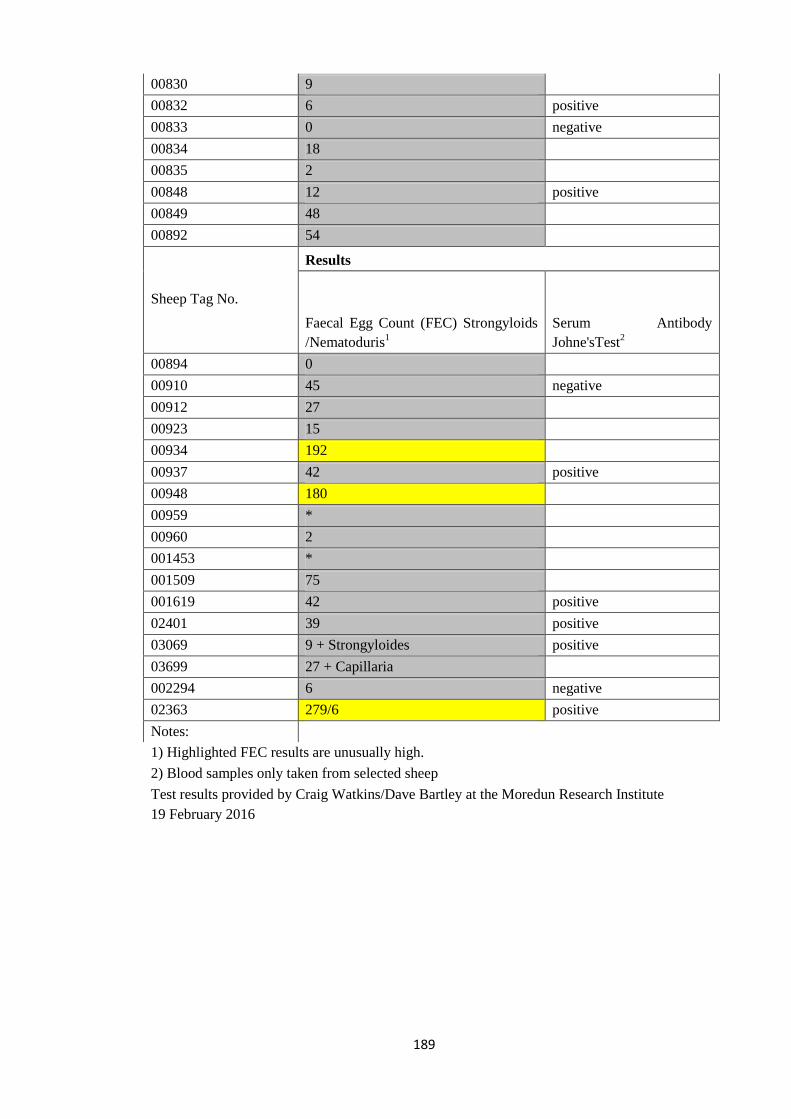
189

00830 9

00832 6 positive

00833 0 negative

00834 18

00835 2

00848 12 positive

00849 48

00892 54

Sheep Tag No.

Results

Faecal Egg Count (FEC) Strongyloids

/Nematoduris1

Serum Antibody

Johne'sTest2

00894 0

00910 45 negative

00912 27

00923 15

00934 192

00937 42 positive

00948 180

00959 *

00960 2

001453 *

001509 75

001619 42 positive

02401 39 positive

03069 9 + Strongyloides positive

03699 27 + Capillaria

002294 6 negative

02363 279/6 positive

Notes:

1) Highlighted FEC results are unusually high.

2) Blood samples only taken from selected sheep

Test results provided by Craig Watkins/Dave Bartley at the Moredun Research Institute

19 February 2016

Documents

Declaration of own work (Research dissertation)