Deconvolution Methods for 3-D Fluorescence Microscopy …

Deconvolution of three-dimensional (3-D) fluorescence microscopy images usingcomputational restoration techniques has attracted great interest in the pastdecades [1]–[3]. Fluorescence microscope imaging properties and measurementimperfections distort the original 3-D image and reduce the maximal resolutionobtainable by the imaging system, thereby restricting the quantitative analysis of

the 3-D specimen [4]. Deconvolution is an operation that mitigates the distortion created by themicroscope. The problem is often ill-posed, since little information on the imaging system isavailable in practice [5]. In this article, we present an overview of various deconvolution tech-niques on 3-D fluorescence microscopy images. We describe the subject of image deconvolutionfor 3-D fluorescence microscopy images and provide an overview of the distortion issues in dif-ferent areas. We introduce a brief schematic description of fluorescence microscope systems andprovide a summary of the microscope point-spread function (PSF), which often creates themost severe distortion in the acquired 3-D image. We discuss our ongoing research work in thisarea. We give a brief review of performance measures of three-dimensional (3-D) deconvolutionmicroscopy techniques and summarize numerical results using simulated data, and then wepresent results obtained from the real data.

IEEE SIGNAL PROCESSING MAGAZINE [32] MAY 2006 1053-5888/06/$20.00©2006IEEE

Deconvolution Methodsfor 3-D FluorescenceMicroscopy Images

[An overview]

[Pinaki Sarder and Arye Nehorai]

©D

IGIT

ALV

ISIO

N, S

MA

LLC

IRC

LE IM

AG

ES

FR

OM

TO

PT

O B

OT

TO

M: L

. SO

US

TE

LLE

, C. J

AC

QU

ES

, AN

D

A. G

IAN

GR

AN

DE

, IG

BM

C, I

LLK

IRC

H, F

RA

NC

E; G

. SC

HE

RR

ER

, P. T

RY

OE

N-T

OT

H, A

ND

B. L

. KIE

FF

ER

, IG

BM

C,

ILLK

IRC

H, F

RA

NC

E; L

. MC

MA

HO

N, J

.-L.

VO

NE

SC

H, A

ND

M. L

AB

OU

ES

SE

, IG

BM

C, I

LLK

IRC

H, F

RA

NC

E.

IEEE SIGNAL PROCESSING MAGAZINE [33] MAY 2006

IMAGE DECONVOLUTION

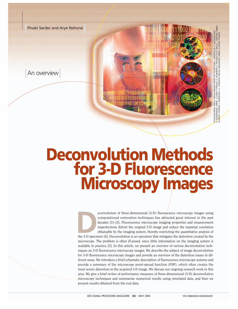
APPLICATIONSIn biomedical research, fluorescence microscopy is widely usedto analyze 3-D structures of living biological cells and tissues[4]. Micro total analysis systems (µTAS) have been developedusing a regenerable microparticle ensemble that could poten-tially determine the existence of hundreds of different targets inbiochemical detection, where quantum dot encoded microparti-cle based arrays (QDEMA) are imaged by using a computer-con-trolled epi-fluorescence microscope [3]. A very similar problemdeals with quantifying the total amount of DNA inside a cellnucleus using fluorescence microscopy imaging. All these treat-ments share a common challenge: imaging systems always dis-tort objects. Image deconvolution restores objects typically bycharacterizing this distortion [6]. Other applications for imagedeconvolution can be found in astronomical speckle imaging,remote sensing, positron-emission tomography, and so on. Forexample, in Figure 1, the captured 3-D fluorescence microscopeimage of a spherical cell stretches along the opticalaxis (z-axis) and maintains its circular shape alongthe radial direction. All two-dimensional (2-D)optical slices have an in-focus plane and a contri-bution from the out-of-focus fluorescence thatobscures the image and reduces contrast [7].

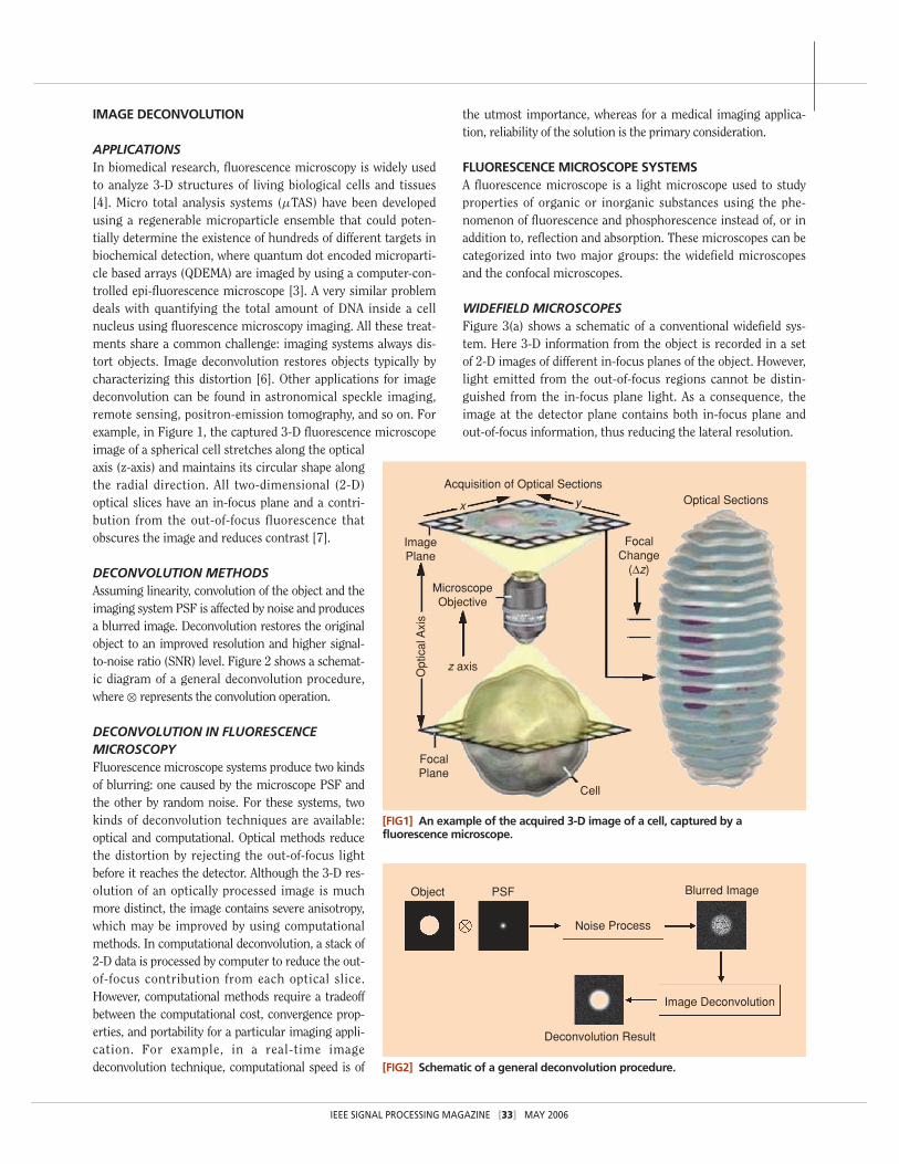
DECONVOLUTION METHODSAssuming linearity, convolution of the object and theimaging system PSF is affected by noise and producesa blurred image. Deconvolution restores the originalobject to an improved resolution and higher signal-to-noise ratio (SNR) level. Figure 2 shows a schemat-ic diagram of a general deconvolution procedure,where ⊗ represents the convolution operation.

DECONVOLUTION IN FLUORESCENCEMICROSCOPYFluorescence microscope systems produce two kindsof blurring: one caused by the microscope PSF andthe other by random noise. For these systems, twokinds of deconvolution techniques are available:optical and computational. Optical methods reducethe distortion by rejecting the out-of-focus lightbefore it reaches the detector. Although the 3-D res-olution of an optically processed image is muchmore distinct, the image contains severe anisotropy,which may be improved by using computationalmethods. In computational deconvolution, a stack of2-D data is processed by computer to reduce the out-of-focus contribution from each optical slice.However, computational methods require a tradeoffbetween the computational cost, convergence prop-erties, and portability for a particular imaging appli-cation. For example, in a real-time imagedeconvolution technique, computational speed is of

the utmost importance, whereas for a medical imaging applica-tion, reliability of the solution is the primary consideration.

FLUORESCENCE MICROSCOPE SYSTEMSA fluorescence microscope is a light microscope used to studyproperties of organic or inorganic substances using the phe-nomenon of fluorescence and phosphorescence instead of, or inaddition to, reflection and absorption. These microscopes can becategorized into two major groups: the widefield microscopesand the confocal microscopes.

WIDEFIELD MICROSCOPESFigure 3(a) shows a schematic of a conventional widefield sys-tem. Here 3-D information from the object is recorded in a setof 2-D images of different in-focus planes of the object. However,light emitted from the out-of-focus regions cannot be distin-guished from the in-focus plane light. As a consequence, theimage at the detector plane contains both in-focus plane andout-of-focus information, thus reducing the lateral resolution.

[FIG1] An example of the acquired 3-D image of a cell, captured by afluorescence microscope.

Optical SectionsAcquisition of Optical Sections

ImagePlane

MicroscopeObjective

FocalPlane

Cell

FocalChange

(∆z)

z axis

Opt

ical

Axi

s

x y

[FIG2] Schematic of a general deconvolution procedure.

Object PSF Blurred Image

Image Deconvolution

Deconvolution Result

Noise Process

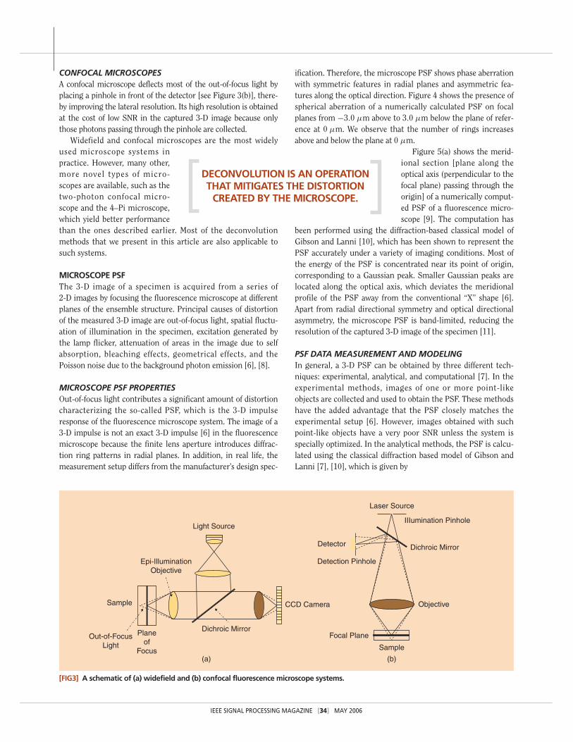
CONFOCAL MICROSCOPESA confocal microscope deflects most of the out-of-focus light byplacing a pinhole in front of the detector [see Figure 3(b)], there-by improving the lateral resolution. Its high resolution is obtainedat the cost of low SNR in the captured 3-D image because onlythose photons passing through the pinhole are collected.

Widefield and confocal microscopes are the most widelyused microscope systems inpractice. However, many other,more novel types of micro-scopes are available, such as thetwo-photon confocal micro-scope and the 4–Pi microscope,which yield better performancethan the ones described earlier. Most of the deconvolutionmethods that we present in this article are also applicable tosuch systems.

MICROSCOPE PSFThe 3-D image of a specimen is acquired from a series of 2-D images by focusing the fluorescence microscope at differentplanes of the ensemble structure. Principal causes of distortionof the measured 3-D image are out-of-focus light, spatial fluctu-ation of illumination in the specimen, excitation generated bythe lamp flicker, attenuation of areas in the image due to selfabsorption, bleaching effects, geometrical effects, and thePoisson noise due to the background photon emission [6], [8].

MICROSCOPE PSF PROPERTIESOut-of-focus light contributes a significant amount of distortioncharacterizing the so-called PSF, which is the 3-D impulseresponse of the fluorescence microscope system. The image of a3-D impulse is not an exact 3-D impulse [6] in the fluorescencemicroscope because the finite lens aperture introduces diffrac-tion ring patterns in radial planes. In addition, in real life, themeasurement setup differs from the manufacturer’s design spec-

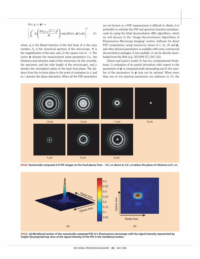
ification. Therefore, the microscope PSF shows phase aberrationwith symmetric features in radial planes and asymmetric fea-tures along the optical direction. Figure 4 shows the presence ofspherical aberration of a numerically calculated PSF on focalplanes from −3.0 µm above to 3.0 µm below the plane of refer-ence at 0 µm. We observe that the number of rings increasesabove and below the plane at 0 µm.

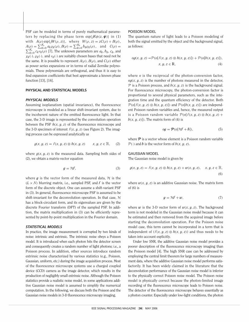
Figure 5(a) shows the merid-ional section [plane along theoptical axis (perpendicular to thefocal plane) passing through theorigin] of a numerically comput-ed PSF of a fluorescence micro-scope [9]. The computation has

been performed using the diffraction-based classical model ofGibson and Lanni [10], which has been shown to represent thePSF accurately under a variety of imaging conditions. Most ofthe energy of the PSF is concentrated near its point of origin,corresponding to a Gaussian peak. Smaller Gaussian peaks arelocated along the optical axis, which deviates the meridionalprofile of the PSF away from the conventional “X” shape [6].Apart from radial directional symmetry and optical directionalasymmetry, the microscope PSF is band-limited, reducing theresolution of the captured 3-D image of the specimen [11].

PSF DATA MEASUREMENT AND MODELINGIn general, a 3-D PSF can be obtained by three different tech-niques: experimental, analytical, and computational [7]. In theexperimental methods, images of one or more point-likeobjects are collected and used to obtain the PSF. These methodshave the added advantage that the PSF closely matches theexperimental setup [6]. However, images obtained with suchpoint-like objects have a very poor SNR unless the system isspecially optimized. In the analytical methods, the PSF is calcu-lated using the classical diffraction based model of Gibson andLanni [7], [10], which is given by


[FIG3] A schematic of (a) widefield and (b) confocal fluorescence microscope systems.

(b)(a)

Laser Source

Detector

Detection Pinhole

Dichroic Mirror

IIIumination Pinhole

Objective

Focal Plane

Sample

Out-of-FocusLight

Planeof

Focus

Epi-IlluminationObjective

Dichroic Mirror

CCD Camera

Light Source

Sample

DECONVOLUTION IS AN OPERATIONTHAT MITIGATES THE DISTORTION

CREATED BY THE MICROSCOPE.


h(x, y, z;ψψψ) =∣∣∣∣∣∣∫ 1

0J0

KNaρ

√x2 + y2

M

exp{ jKφ(z,ψψψ)}ρdρ

∣∣∣∣∣∣2

, (1)

where J0 is the Bessel function of the first kind, K is the wavenumber, Na is the numerical aperture of the microscope, M isthe magnification of the lens, and j is the square root of −1. The vector ψψψ denotes the measurement setup parameters (i.e., thethickness and refractive index of the immersion oil, the coverslip,the specimen, and the tube length of the microscope), and ρdenotes the normalized radius in the back focal plane. The dis-tance from the in-focus plane to the point of evaluation is z, andφ(·) denotes the phase aberration. When all the PSF parameters

are not known or a PSF measurement is difficult to obtain, it ispreferable to estimate the PSF and specimen function simultane-ously by using the blind deconvolution (BD) algorithms, whichwe will discuss in the “Image Deconvolution Algorithms ofFlourescence Microscopy Imaging” section. Software for directPSF computation using numerical values of λ, Na, M, and ψψψ ,and other physical parameters is available with some commercialdeconvolution packages; if not available, it can be directly down-loaded from the Web (e.g., XCOSM) [7], [10], [12].

Gibson and Lanni’s model (1) has two computational limita-tions: 1) evaluation of its partial derivatives with respect to theparameters of ψψψ is computationally demanding and 2) the num-ber of the parameters in ψψψ may not be optimal. When morethan one or two physical parameters are unknown in (1), the

[FIG4] Numerically computed 2-D PSF images on the focal planes from −3.0 µm above to 3.0 µm below the plane of reference at 0 µm.

−3 µm

3 µm2 µm1 µm

−2 µm −1 µm 0 µm

[FIG5] (a) Meridional section of the numerically computed PSF of a fluorescence microscope with the signal intensity represented byheight; (b) projected top view of the signal intensity of the PSF in the meridional section.

(a) (b)

Radial Axis

0.4

0.35

0.3

0.25

0.2

0.15

0.1

0.05

Optical Axis

Radial Axis

Opt

ical

Axi

s

PSF can be modeled in terms of purely mathematical parame-ters by replacing the phase term exp{ jKφ(z,ψψψ)} in (1) with A(ρ) exp{ jW(ρ, z)} , where W(ρ, z) = zC(ρ) + B(ρ) ,A(ρ) = ∑Ka

k=0 akχk(ρ), B(ρ) = ∑Kbk=0 bk�k(ρ) , and C(ρ) =∑Kc

k=0 ckνk(ρ) [7]. The unknown parameters are ak, bk, ck, andχk(·), �k(·), and νk(·) are suitably chosen bases that need not bethe same. It is possible to represent A(ρ), B(ρ), and C(ρ) eitheras power series expansions or in terms of radial Zernike polyno-mials. These polynomials are orthogonal, and thus it is easy tofind expansion coefficients that best approximate a known phasefunction [13], [14].

PHYSICAL AND STATISTICAL MODELS

PHYSICAL MODELSAssuming isoplanatism (spatial invariance), the fluorescencemicroscope is modeled as a linear shift-invariant system, due tothe incoherent nature of the emitted fluorescence light. In thatcase, the 3-D image is represented by the convolution operationbetween the PSF h(x, y, z) of the fluorescence microscope andthe 3-D specimen of interest f(x, y, z) (see Figure 2). The imag-ing process can be expressed analytically as

g(x, y, z) = f(x, y, z) ⊗ h(x, y, z) x, y, z ∈ R, (2)

where g(x, y, z) is the measured data. Sampling both sides of(2), we obtain a matrix-vector equation

g = Hf , (3)

where g is the vector form of the measured data, H is the(L × N) blurring matrix, i.e., sampled PSF, and f is the vectorform of the discrete object. One can assume a shift-variant PSFin (3). In general, fluorescence microscope PSF is assumed to beshift-invariant for the deconvolution operation. In that case, Hhas a block-circulant form, and its eigenvalues are given by thediscrete Fourier transform (DFT) of the sampled PSF. In addi-tion, the matrix multiplication in (3) can be efficiently repre-sented by point-by-point multiplication in the Fourier domain.

STATISTICAL MODELSIn practice, the image measurement is corrupted by two kinds ofnoise: intrinsic and extrinsic. The intrinsic noise obeys a Poissonmodel. It is introduced when each photon hits the detector screenand consequently creates a random number of light photons; i.e., aPoisson process. In addition, other sources introduce randomextrinsic noise characterized by various statistics (e.g., Poisson,Gaussian, uniform, etc.) during the image acquisition process. Mostof the fluorescence microscope systems use a charged coupleddevice (CCD) camera as the image detector, which results in theproduction of negligibly small extrinsic noise. Although the Poissonstatistics provide a realistic noise model, in some applications addi-tive Gaussian noise model is assumed to simplify the numericalcomputation. In the following, we discuss both the Poisson and theGaussian noise models in 3-D fluorescence microscopy imaging.

POISSON MODELThe quantum nature of light leads to a Poisson modeling ofboth the signal emitted by the object and the background signal,as follows:

og(x, y, z) =P(o[ f(x, y, z) ⊗ h(x, y, z)]) + P(o[b(x, y, z)]),

x, y, z ∈ R, (4)

where o is the reciprocal of the photon-conversion factor,og(x, y, z) is the number of photons measured in the detector,P is a Poisson process, and b(x, y, z) is the background signal.For fluorescence microscopy, the photon-conversion factor isproportional to several physical parameters, such as the inte-gration time and the quantum efficiency of the detector. BothP(o[ f(x, y, z) ⊗ h(x, y, z)]) and P(o[b(x, y, z)]) are independ-ent Poisson random variables and, hence, the measured outputis a Poisson random variable P(o[ f(x, y, z) ⊗ h(x, y, z) +b(x, y, z)]). The matrix form of (4) is

og = PPP(o[Hf + b]), (5)

where PPP is a vector whose element is a Poisson random variableP(·) and b is the vector form of b(x, y, z).

GAUSSIAN MODELThe Gaussian noise model is given by

g(x, y, z) = f(x, y, z) ⊗ h(x, y, z) + w(x, y, z), x, y, z ∈ R,

(6)

where w(x, y, z) is an additive Gaussian noise. The matrix formof (6) is

g = Hf + w, (7)

where w is the 3-D vector form of w(x, y, z). The backgroundterm is not modeled in the Gaussian noise model because it canbe estimated and then removed from the acquired image beforestarting the deconvolution operation. For the Poisson noisemodel case, this term cannot be incorporated in a term that isindependent of ( f(x, y, z) ⊗ h(x, y, z)) and thus needs to betaken into account explicitly.

Under low SNR, the additive Gaussian noise model provides apoorer description of the fluorescence microscopy imaging thanthe Poisson model [4]. The high SNR case can be addressed byemploying the central limit theorem for large numbers of measure-ment data, where the additive Gaussian noise model performs satis-factorily. It has been widely claimed in the literature that thedeconvolution performance of the Gaussian noise model is inferiorto the physically correct Poisson noise model. The Poisson noisemodel is physically correct because the photon-limited imagerecording of the fluorescence microscope leads to Poisson noise.The detector of the fluorescence microscope behaves essentially asa photon counter. Especially under low-light conditions, the photon



number is generally extremely small, and the statistical variation inthe number of detected photons is best described by a Poisson mod-eling of the noise. In addition, it is assumed that the Poisson noisemodel leads to a faster convergence of the object function.

IMAGE DECONVOLUTION ALGORITHMS OF FLUORESCENCE MICROSCOPY IMAGINGThe computational 3-D image deconvolution techniques can be cat-egorized into six broad classes: no-neighbors methods, neighboringmethods, linear methods, nonlinear methods, statistical methods,and BDs. Often, the raw 3-D image data contain nonuniform spatialillumination and uneven sensitivity imposed by the CCD camera.To correct those errors, an image smoothing operation called flatfielding is necessary. Flat fielding is done by imaging a uniformly flu-orescent object (such as fluorescent plastic) and then using the fluc-tuations in this image to calibrate the uneven illumination.

NO-NEIGHBORS METHODSThese computationally efficient methods process each 2-D focalplane slice separately. Applications of such methods are limitedto high-spatial-frequency objects [6], [15].

NEIGHBORING METHODSThe next computationally efficient and simplest methods are theneighboring methods. These methods are classified into twogroups: the nearest-neighbors methods and the multineighborsmethods. In the nearest-neighbors methods, each 2-D focal planeimage is deblurred by considering information from two adjacentplanes. Focal planes above and below the plane of interest areblurred by using a digital blurring filter. After that, deconvolutionis performed by subtracting the blurred planes from the focalplane image [1]. Such methods work satisfactorily when a signifi-cant amount of blur in the focal plane image is contributed by theadjacent planes. Multineighbors methods extend the nearest-neighbors methods by considering a number of user-definedplanes. While the neighboring methods sharpen the 3-D image,they have several disadvantages. For one, they are not efficient atremoving the noise. For another, these methods introduce struc-tural artifacts. Care is required while applying these methods,especially for morphometric measurements, quantitative fluores-cence measurements, and intensity ratio calculations.

LINEAR METHODSThe simplest and truest 3-D methods for deconvolution use theinformation from all the focal planes. Deterministic blurring ismodeled by (2) and (3). Some linear methods (e.g., the Wienerfiltering method) assume additive Gaussian noise [(6) and (7)]for the corresponding 3-D image deconvolution operation.

INVERSE FILTERINGThe image distortion model in (2) is assumed without furtherassumptions on noise statistics. For a known h(x, y, z), the 3-D deconvolved image of the specimen is given by [6]f(x, y, z) = F−1(G(ωx, ωy, ωz))/(H(ωx, ωy, ωz)}), whereωx, ωy, and ωz denote the frequency domain counterparts of the

space variables x, y, and z, respectively; G(ωx, ωy, ωz) andH(ωx, ωy, ωz) are the 3-D Fourier transforms of g(x, y, z) andh(x, y, z); f(x, y, z) is the deconvolved image of the specimen in3-D; and F−1 is the inverse Fourier transform operation in 3-D.The PSF is band-limited, therefore at high spatial frequency thedenominator of G(ωx, ωy, ωz)/H(ωx, ωy, ωz) is close to zeroand the inverse filtering method suffers from severe noise ampli-fication [6]. This problem can be tackled by using a truncatedinverse filter given by

f(x, y, z) ={

F−1{

G(ωx,ωy,ωz)

H(ωx,ωy,ωz)

}if |H(ωx, ωy, ωz)| ≥ ε

0 if |H(ωx, ωy, ωz)| ≤ ε,

(8)

where ε is a small positive constant.

WIENER FILTERINGThe image distortion model in (6) is considered for signal-independent additive Gaussian noise. For a known h(x, y, z),g(x, y, z) in (6) is deconvolved as f(x, y, z) = g(x, y, z)⊗ h(x, y, z) , where x, y, z ∈ R and h(x, y, z) is the mean-square error (MSE)-optimal stationary linear filter forthe deconvolution. In the frequency domain, h(x, y, z) isgiven as H(ωx, ωy, ωz) = H∗(ωx, ωy, ωz)/{|H(ωx, ωy, ωz)|2+(Pw(ωx, ωy, ωz)/Pf (ωx, ωy, ωz))}, where H(ωx, ωy, ωz) is the3-D Fourier transform of h(x, y, z), “∗’’ is the complex conjuga-tion operation, and Pw(ωx, ωy, ωz) and Pf (ωx, ωy, ωz) are thepower spectral densities of the noise and the specimen, respec-tively [16]–[17].

LINEAR LEAST SQUARES METHODThe linear least squares (LLS) method assumes the image dis-tortion model (2) and (3). For the sake of clarity, we follow thematrix equation (3). The least-squares solution of (3) is given asf = (HTH)

−1HTg, where f denotes the estimated 3-D image invector form after the deconvolution operation. The blurringmatrix H might not be of full column rank and, hence, HTHmight not have an inverse [18].

TIKHONOV FILTERINGThe same image distortion model is assumed as in the LLSmethod. Direct minimization of ||Hf − g||2 (|| · || is theEuclidean norm) for a known H in the LLS method producesundesired results since it does not restore high-frequency components of the specimen. Therefore, the authors in [5] suggest minimizing the Tikhonov functional �(f ) =||Hf − g||2 + λ||C f ||2, where λ is the regularization parameterand C is the regularization matrix. The matrix C penalizes thesolution of f in the regions where it oscillates due to the spectralcomponents dominated by noise. In matrix notation f is given asf = (HTH + λCTC)

−1HTg.Wiener, LLS, and Tikhonov filtering do not restore the origi-

nal specimen’s frequency components beyond the PSF band-width. Sometimes, linear methods estimate negative intensity in

the deconvolved image. In addition, these methods are very sen-sitive to errors in the PSF data used for the estimation, causinga ringing artifact in the deconvolved 3-D image.

NONLINEAR METHODSTo solve the difficulties encountered in the linear methods, addi-tional physical information (e.g., nonnegativity, finite specimensupport, specimen smoothness, and regularization) is incorpo-rated, yielding nonlinear iterative algorithms at the cost ofincreased computational complexity.

JANSON VAN CITTERT ALGORITHMHistorically, the Janson Van Cittert (JVC) algorithm was the firstiterative method for constrained deconvolution. At each itera-tion, an error image is calculated by subtracting the estimatedimage from the recorded distorted image. To prevent negativeintensities or very bright intensities, the error image is multi-plied by a finite weight function that is defined over a positiveintensity band. Finally, the weighted error is subtracted fromthe specimen estimate to obtain the new estimate. This methodamplifies high-frequency noise at each iteration and thusrequires a smoothing step at each iteration. Unfortunately, thesmoothing operation does not work well for low SNR images.While JVC improves the resolution in the final estimated image,this method is not good for removing the noise [1].

NONLINEAR LEAST-SQUARES METHODIn JVC, the error between the recorded image and the estimatedimage can be negative. In the nonlinear least-squares (NLS)approach, the sum of the squared error between the recordeddistorted image and the estimated image is minimized by incor-porating a nonnegativity constraint, where either negativeintensities are set to zero values or the specimen is constrainedto be positive [19].

ITERATIVE CONSTRAINEDTIKHONOV-MILLER ALGORITHM In the iterative constrained Tikhonov-Miller algorithm (ICTM)approach, the minimum of �(f ) is searched iteratively by clip-ping the estimated negative intensities to zero after each itera-tion. In general, a conjugate gradient (CG) method is used forthe iterative search operation. CG computes a path in thedirection of the minimum of �(f ) after an initial downhillstep. CG direction is given as dk = rk + ξkdk−1, where for thekth iteration ξk = ||rk||2/||rk−1||2 and rk is the steepestdescent (SD) direction, given by rk = (−1/2)�

f�(f ) =

(HTH + λCTC )fk − HTg. Finally, the CG estimate is

fk+1 ={

fk + ιkdk if fk + ιkdk ≥ 00 otherwise,

(9)

where ιk is the optimal step size. In the absence of any nonneg-ativity constraint, ιk can be computed analytically; otherwise,the iterative golden section rule searches for an optimum ιk ineach iteration. The computational speed of the ICTM algorithm

is dominated by the search for ιk performed at each iteration [4],[8], [20]. A modified version of the ICTM algorithm, theCarrington algorithm, achieves minimization using the Kuhn-Tucker condition. The result of the ICTM algorithm is overlysmooth when the regularization parameter λ is close to 1/SNR.Higher values of λ produce smoother results. Three reliablemethods are available for determining the λ parameter, namely,constrained least squares, generalized cross validation, and max-imum likelihood [4], [21], [22].

LLS, Tikhonov filtering, NLS, ICTM, and the Carrington algo-rithm are based on the assumption that the general noise distor-tion function can be modeled as additive Gaussian noise.However, these methods do not have a direct noise-reductionstrategy. Nonetheless, statistical processing with necessary physi-cal constraints would eliminate both the out-of-focus light andrandom noise and, thus, improve the deconvolution performance.

STATISTICAL METHODSThese methods are extremely effective when the noise in theacquired 3-D image is fairly strong [6]. These methods have a moresubtle noise strategy than the simple regularizations. They are alsohelpful in obtaining certain information not captured by the micro-scope optics [6]. However, they are more complex and computa-tionally more intensive than the linear and nonlinear methods.

MAXIMUM LIKELIHOOD METHODSMaximum likelihood (ML) methods have the apparent charac-teristic of restoring good-quality images in the presence of highnoise levels. For the additive Gaussian noise models in (6) and(7), the ML solution is essentially the LLS solution for a knownh(x, y, z), assuming the noise is signal independent. To obtainthe ML estimate of f(x, y, z), the likelihood function for thePoisson imaging model in (4) is maximized as J( f) =∑

x∑

y∑

z {g(x, y, z) log[ f (x, y, z)⊗h(x, y, z) + b(x, y, z)] −( f(x, y, z)⊗h(x, y, z))}. To apply classical ML estimation, bothh(x, y, z) and f(x, y, z) are required to be in parametric form.When h(x, y, z) is known and b(x, y, z) is omitted, a multiplica-tive gradient-based iterative search algorithm maximizes J( f )

and yields the following iterative algorithm,

fi+1(x, y, z) ={[

g(x, y, z)

fi(x, y, z)⊗h(x, y, z)

]⊗ h(−x,−y,−z)

}

× fi(x, y, z), (10)

where fi(·) is the estimation of the object at the i th iteration. Theiterative form (10) ensures nonnegativity for a nonnegativeinitial guess f0(·). An expectation maximization (EM) algorithmfor the ML estimation can also produce the same solution for theobject estimation as given in (10). For conciseness, we summarizethe philosophy behind the EM approach rather than giving thedetailed derivations. In the EM algorithm, two data sets aredefined for the ML estimation: the unobservable complete data setand the observable incomplete data set. In 3-D fluorescencemicroscopy, the complete data set is commonly defined as thespecimen function f(x, y, z) to be estimated and the incomplete



data set is defined as the recorded image g(x, y, z). The first step(E-step) finds the expected value of the complete-data log-likeli-hood of (4) with respect to the conditional probability densityfunction (pdf) of the complete data set given the incomplete dataset g(x, y, z) [7]. The second step (M-step) maximizes the expec-tation that is computed in the E-step. However, because the 3-Ddeconvolution process is ill-posed, the iterative solution given by(10) converges to noise asymptotically, which can be removed fur-ther by using regularization techniques [11]. The EM algorithmhas a slow rate of convergence, and the computation is intensive[23]–[25]. We present a new approach using parametric modelwith ML estimation method for deconvolution of 3-D fluores-cence microscopy images at the end of this section.

MAXIMUM A POSTERIORI METHODThe ML estimation can be easily extended to the maximum aposteriori (MAP) method based on realistic prior knowledge ofthe object. From (5) and (7), we write in terms of Bayesian ter-minology, p(f |g) = p(g|f )p(f )/p(g), where p(f ) denotes thepdf of f and p(f |g) denotes the conditional pdf of f given g. TheMAP solution is obtained by maximizing p(g|f )p(f ) . TheGaussian prior distribution of the object is given byp(f ) = kexp(−1/(2τ 2)||C (f − m)||2) , where m is the priorknowledge of the shape of the object, C is the regularizationmatrix based on the constraints, τ 2 is the variance of the priorGaussian distribution, and k is a normalizing constant. In theabsence of further prior knowledge, the entropy distribution isthe only consistent prior distribution for positive additiveimages. The entropy function S is defined byS(x, y) = ∑M

i=1(xi − yi − xi ln (xi/yi)) , where the model yreflects the prior knowledge of x and xi, yi are the i th elementsof vectors x and y. The global maximum of S(·) is y and, hence,y is the most likely value of x according to the entropy distribu-tion. The entropy prior distribution of the object is given byp(f ) = kexp(ζ S(|C f |, |Cm|)), where the absolute value | · | isapplied to each element of |C f | and |Cm|, corresponding to theassumption that the absolute values of linear combinations ofpixels have an entropy distribution. The arbitrary constants aredenoted by k and ζ . The conditional distribution p(g|f ) can beboth Gaussian or Poisson distributed, according to (5) or (7).Assuming a Gaussian or Poisson noise model and either aGaussian or an entropy prior distribution for the object, MAPestimates are produced by minimizing functionals ς(f ) as dis-cussed in Table 1, where � is the regularization parameter anddivisions of vectors are performed element by element.Similarly, a Poisson prior of the object can be assumed and thecorresponding functional ς(f ) can be formed. The parameter �determines the tradeoff between the amount of smoothing andfitting accuracy. The roots of the gradients of the functionalsς(f ) are searched iteratively by using a CG algorithm [26]–[28].

BLIND DECONVOLUTION METHODSPerformance of all the previous algorithms depends on accurate PSFmodeling, which is a challenging task in a real imaging scenario.Noise is always present in an experimentally measured PSF, whereas

a theoretical PSF cannot completely determine all aberrations pres-ent in microscope optics. Blind deconvolution (BD) methods simul-taneously estimate the microscope PSF and the original 3-Dspecimen image [6]. The following brief review of the BD algorithmis based on the Richardson-Lucy (RL) algorithm, which adopts thePoisson noise model. The RL algorithm can be given in one dimen-sion as fi+1(α) = {∫ h(β, α)g(β)dβ/

∫h(β, γ ) fi(γ )dγ } fi(α) ,

where α and β are two events, fi(α) is the object distribution at thei th iteration, h(β, α) is the PSF centered at α, and the degradedimage is g(β). Assuming an isoplanatic condition and extending theproblem into 3-D, we derive (10) from (2) and f(·)(α). The blindform of (10) can be written as

hki+1(x, y, z) =

{[g(x, y, z)

h ki (x, y, z)⊗ f k−1(x, y, z)

]

⊗ f k−1(−x,−y,−z)

}hk

i (x, y, z),

f ki+1(x, y, z) =

{[g(x, y, z)

f ki (x, y, z)⊗hk−1(x, y, z)

]

⊗ hk−1(−x,−y,−z)

}f ki (x, y, z), (11)

where at the kth blind iteration it is assumed that the PSF is knownfrom the (k − 1)th iteration. The object f k(x, y, z) is then calcu-lated for a specified number of RL iterations as in (11), where theindex i represents RL iteration. The PSF hk(x, y, z) is then calculat-ed from (11) for the same number of RL iterations. This algorithmautomatically satisfies a priori image-domain constraints (i.e., posi-tivity, energy conservation, and support constraint [29]) while con-verging towards the ML solution. In [24], only two RL iterations areperformed within one blind iteration, one for the object and one forthe PSF evaluation, which does not perform well on simulatedexamples [29]. The RL algorithm is very sensitive to noise. To reducethe noise sensitivity, the high-frequency parts (i.e., low SNR regions)of the object are suppressed by convolving the recorded image witha Gaussian function. This preconvolution operation causes smooth-ing in the RL algorithm and is further compensated by convolvingthe PSF with the same Gaussian [4]. The literature on BD aboundsin variations of the iterative algorithm presented in (11) (e.g., simu-lated annealing, error metric minimization, ML method, EM algo-rithm, etc.). However, all those cases are governed by the samephilosophy, i.e., simultaneous estimation of the object and the PSFin an iterative fashion [7], [30]–[32].

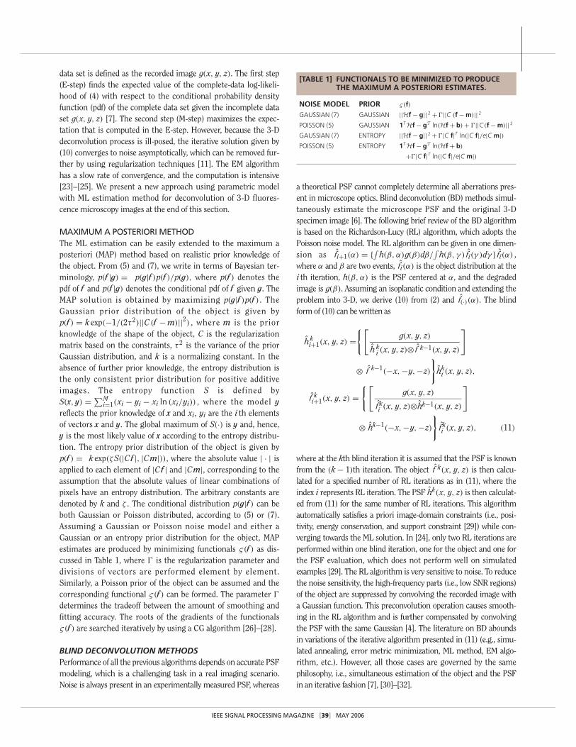
NOISE MODEL PRIOR ς(f)

GAUSSIAN (7) GAUSSIAN ||Hf − g|| 2 +�||C (f − m)|| 2

POISSON (5) GAUSSIAN 1T Hf − gT ln(Hf + b) + �||C (f − m)|| 2

GAUSSIAN (7) ENTROPY ||Hf − g|| 2 +�|C f|T ln(|C f|/e|C m|)POISSON (5) ENTROPY 1T Hf − gT ln(Hf + b)

+�|C f|T ln(|C f|/e|C m|)

[TABLE 1] FUNCTIONALS TO BE MINIMIZED TO PRODUCE THE MAXIMUM A POSTERIORI ESTIMATES.

Care should be taken to avoid nonuniqueness of the BD solu-tion. Even if the solution in (11) is constrained to be nonnega-tive, (2) has two trivial solutions, { f(x, y, z), h(x, y, z)} ={g(x, y, z), δ(x, y, z)} and { f(x, y, z), h(x, y, z)} = {δ(x, y, z),g(x, y, z)}. Similarly, other nonunique solutions also exist, e.g.,{Kf(x, y, z), h(x, y, z)/K} is a solution of (2) for any K > 0.Trivial solutions can be avoided by considering the PSF to becircularly symmetric with a finite frequency domain support.The scaled induced nonuniqueness is avoided by constrainingthe volume integral of the PSF to be finite [24].

In [7], the authors propose a parametric BD technique basedon an iterative algorithm, and the parametric model from (1) isused to avoid the nonunique solutions. The PSF model in (1)automatically satisfies all the physical constraints. In the k thiteration of the algorithm, either the object function f(x, y, z) isestimated by using (10) while keeping the vector of the PSFparameters constant (ψψψ = ψψψ

(k)) or the PSF parameters are

updated numerically while keeping the object function constant.Another well-known method is the BD technique based on thepenalized ML method. With this method, the likelihood is penal-

ized in order to achieve a higher accuracy [33]. However, care isneeded in the selection of penalty terms, since they significantlyaffect the estimates.

WAVELET-BASED PROCESSINGFine details of the 3-D captured image are more sensitive to noise,mismatches in the PSF, under sampling, etc., than are the largerfeatures. Wavelet analysis can perform quite well by analyzing thedifferent scales separately in the deconvolution process. However,development of a 3-D deconvolution scheme using wavelets is stillunexplored because the inverse kernel is known only approximate-ly, a situation routinely encountered in 3-D microscopy. Anapproximate PSF model makes it attractive to propose a computa-tionally efficient wavelet deconvolution scheme dealing with huge3-D images. However, wavelet denoising methods can act as anefficient regularization scheme for 3-D deconvolution, enablinghigher resolution. These methods not only keep the frequencybandwidth of the final restored image nonincreasing, but also sup-press many of the artifacts that would be present at a given step ofdeconvolution without denoising. In general, in combination withmore classical deconvolution algorithms, wavelet denoising meth-ods can provide a robust and efficient deconvolution scheme [34].

COMMERCIAL DECONVOLUTION PACKAGESCommercial deconvolution software packages are available byAutoQuant Imaging, VayTek, Scanalytics, Intelligent ImagingInnovations, and Applied Precision, to name a few. Many ofthese packages include numerous features such as deblurringalgorithms of 3-D fluorescence microscopy images, generat-ing 3-D PSF of fluorescence microscope, etc. The noncom-mercial software package XCOSM can be downloaded fromthe Web directly as free open source code, which runs onUnix-based systems. Developers of XCOSM are working onenhancing the performance and efficiency of this software

with a new software package OMRF-COSM that will run under Windows,Mac OS X, and Linux [12].

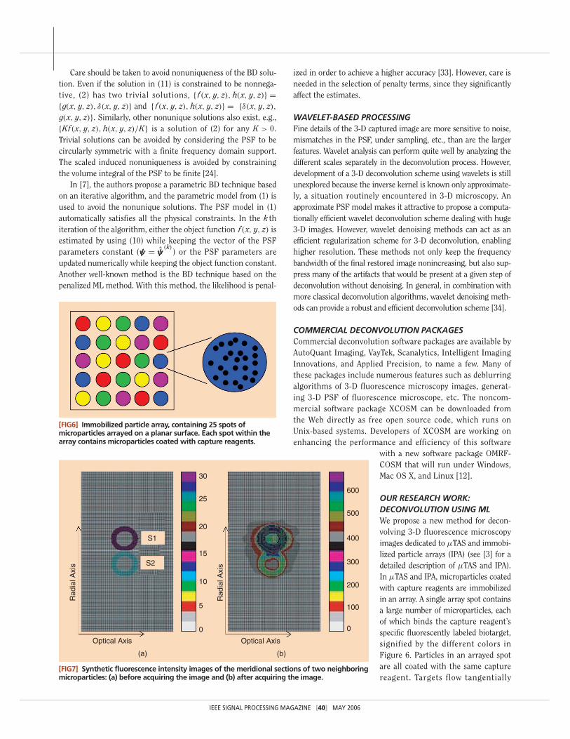
OUR RESEARCH WORK:DECONVOLUTION USING MLWe propose a new method for decon-volving 3-D fluorescence microscopyimages dedicated to µTAS and immobi-lized particle arrays (IPA) (see [3] for adetailed description of µTAS and IPA).In µTAS and IPA, microparticles coatedwith capture reagents are immobilizedin an array. A single array spot containsa large number of microparticles, eachof which binds the capture reagent’sspecific fluorescently labeled biotarget,signified by the different colors inFigure 6. Particles in an arrayed spotare all coated with the same capturereagent. Targets flow tangentially


[FIG6] Immobilized particle array, containing 25 spots ofmicroparticles arrayed on a planar surface. Each spot within thearray contains microparticles coated with capture reagents.

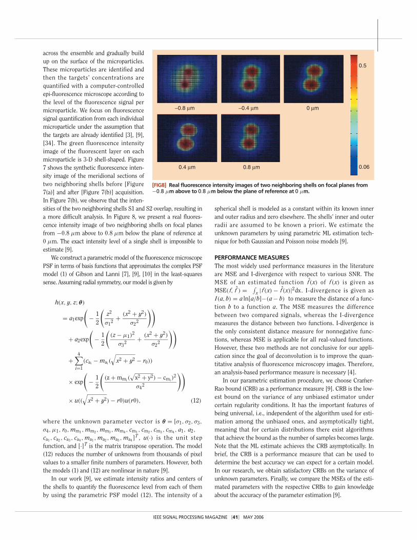
[FIG7] Synthetic fluorescence intensity images of the meridional sections of two neighboringmicroparticles: (a) before acquiring the image and (b) after acquiring the image.

Rad

ial A

xis

Rad

ial A

xis

S1

S2

Optical Axis Optical Axis

(b)(a)

30

25

20

15

10

5

0

600

500

400

300

200

100

0


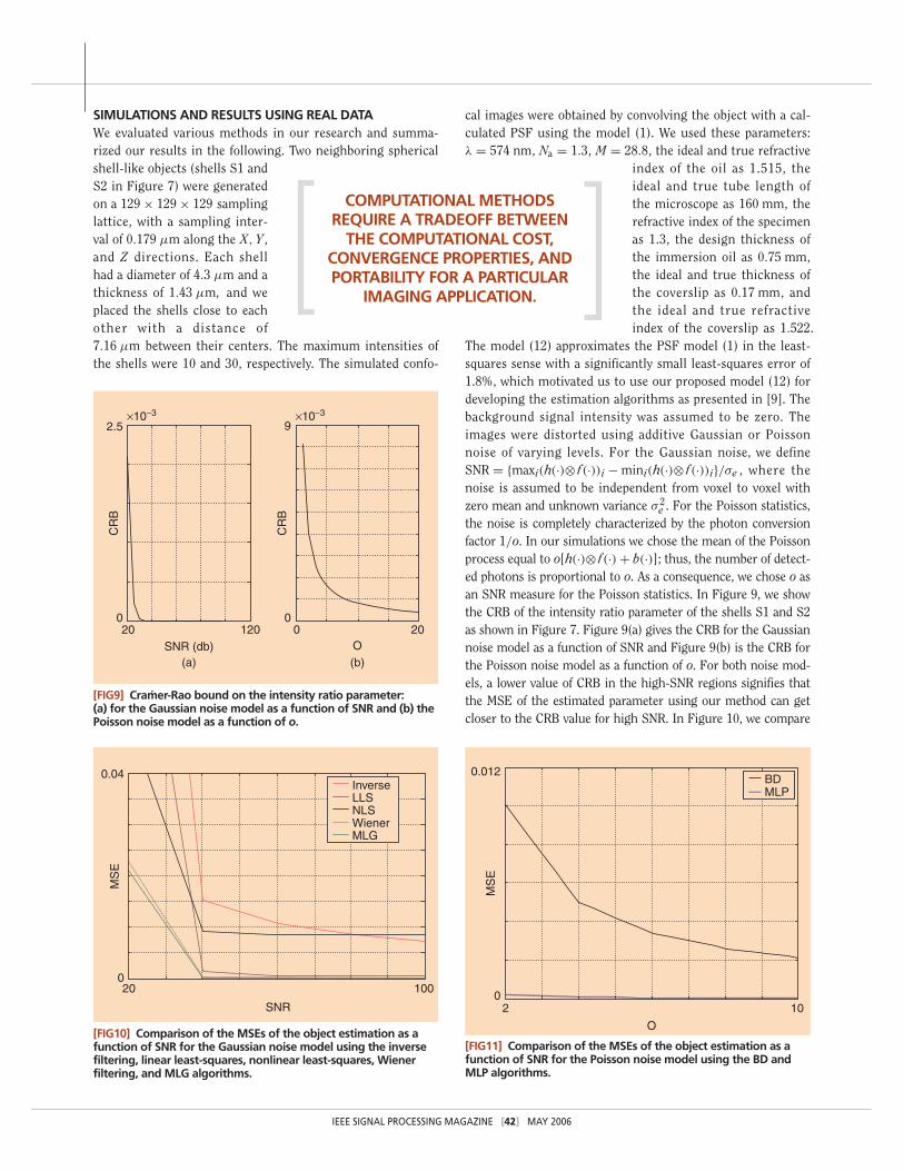
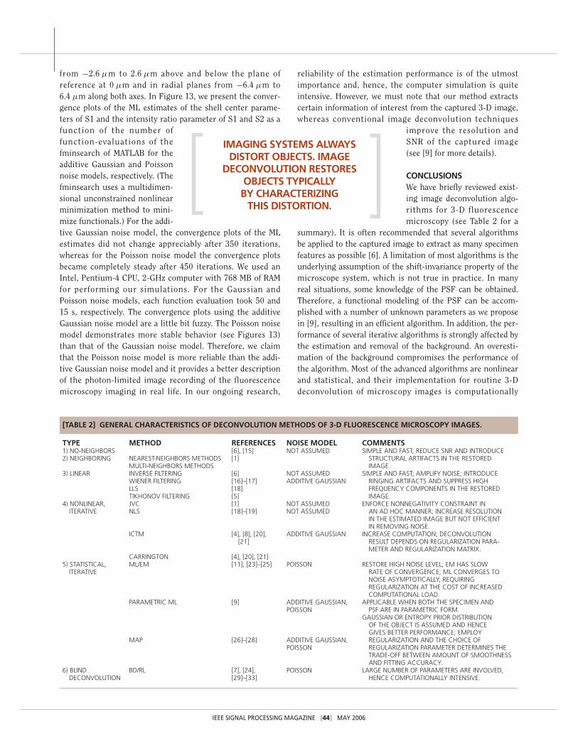
across the ensemble and gradually buildup on the surface of the microparticles.These microparticles are identified andthen the targets’ concentrations arequantified with a computer-controlledepi-fluorescence microscope according tothe level of the fluorescence signal permicroparticle. We focus on fluorescencesignal quantification from each individualmicroparticle under the assumption thatthe targets are already identified [3], [9],[34]. The green fluorescence intensityimage of the fluorescent layer on eachmicroparticle is 3-D shell-shaped. Figure7 shows the synthetic fluorescence inten-sity image of the meridional sections oftwo neighboring shells before [Figure7(a)] and after [Figure 7(b)] acquisition.In Figure 7(b), we observe that the inten-sities of the two neighboring shells S1 and S2 overlap, resulting ina more difficult analysis. In Figure 8, we present a real fluores-cence intensity image of two neighboring shells on focal planesfrom −0.8 µm above to 0.8 µm below the plane of reference at0 µm. The exact intensity level of a single shell is impossible toestimate [9].

We construct a parametric model of the fluorescence microscopePSF in terms of basis functions that approximates the complex PSFmodel (1) of Gibson and Lanni [7], [9], [10] in the least-squaressense. Assuming radial symmetry, our model is given by

h(x, y, z; θθθ)

= a1exp

(− 1

2

(z2

σ12 + (x2 + y2)

σ22

))

+ a2exp

(− 1

2

((z − µ1)

2

σ32 + (x2 + y2)

σ22

))

+4∑

i=1

(cai − mai(

√x2 + y2 − r0))

× exp

(− 1

2

((z + mmi(

√x2 + y2) − cmi)

2

σ42

))

× u((

√x2 + y2) − r0)u(r0), (12)

where the unknown parameter vector is θθθ = [σ1, σ2, σ3,

σ4, µ1, r0, mm1 , mm2 , mm3 , mm4 , cm1 , cm2 , cm3 , cm4 , a1, a2,

ca1 , ca2 , ca3 , ca4 , ma1 , ma2 , ma3 , ma4 ]T , u(·) is the unit stepfunction, and [·]T is the matrix transpose operation. The model(12) reduces the number of unknowns from thousands of pixelvalues to a smaller finite numbers of parameters. However, boththe models (1) and (12) are nonlinear in nature [9].

In our work [9], we estimate intensity ratios and centers ofthe shells to quantify the fluorescence level from each of themby using the parametric PSF model (12). The intensity of a

spherical shell is modeled as a constant within its known innerand outer radius and zero elsewhere. The shells’ inner and outerradii are assumed to be known a priori. We estimate theunknown parameters by using parametric ML estimation tech-nique for both Gaussian and Poisson noise models [9].

PERFORMANCE MEASURESThe most widely used performance measures in the literatureare MSE and I-divergence with respect to various SNR. TheMSE of an estimated function f(x) of f(x) is given asMSE( f, f ) = ∫

x | f(x) − f(x)|2dx. I-divergence is given asI(a, b) = a ln[a/b]−(a − b) to measure the distance of a func-tion b to a function a. The MSE measures the differencebetween two compared signals, whereas the I-divergencemeasures the distance between two functions. I-divergence isthe only consistent distance measure for nonnegative func-tions, whereas MSE is applicable for all real-valued functions.However, these two methods are not conclusive for our appli-cation since the goal of deconvolution is to improve the quan-titative analysis of fluorescence microscopy images. Therefore,an analysis-based performance measure is necessary [4].

In our parametric estimation procedure, we choose Cramer-Rao bound (CRB) as a performance measure [9]. CRB is the low-est bound on the variance of any unbiased estimator undercertain regularity conditions. It has the important features ofbeing universal, i.e., independent of the algorithm used for esti-mation among the unbiased ones, and asymptotically tight,meaning that for certain distributions there exist algorithmsthat achieve the bound as the number of samples becomes large.Note that the ML estimate achieves the CRB asymptotically. Inbrief, the CRB is a performance measure that can be used todetermine the best accuracy we can expect for a certain model.In our research, we obtain satisfactory CRBs on the variance ofunknown parameters. Finally, we compare the MSEs of the esti-mated parameters with the respective CRBs to gain knowledgeabout the accuracy of the parameter estimation [9].

[FIG8] Real fluorescence intensity images of two neighboring shells on focal planes from−0.8 µm above to 0.8 µm below the plane of reference at 0 µm.

−0.8 µm −0.4 µm 0 µm

0.5

0.060.4 µm 0.8 µm

SIMULATIONS AND RESULTS USING REAL DATAWe evaluated various methods in our research and summa-rized our results in the following. Two neighboring sphericalshell-like objects (shells S1 andS2 in Figure 7) were generatedon a 129 × 129 × 129 samplinglattice, with a sampling inter-val of 0.179 µm along the X, Y ,and Z directions. Each shellhad a diameter of 4.3 µm and athickness of 1.43 µm, and weplaced the shells close to eachother with a distance of7.16 µm between their centers. The maximum intensities ofthe shells were 10 and 30, respectively. The simulated confo-

cal images were obtained by convolving the object with a cal-culated PSF using the model (1). We used these parameters:λ = 574 nm, Na = 1.3, M = 28.8, the ideal and true refractive

index of the oil as 1.515, theideal and true tube length ofthe microscope as 160 mm, therefractive index of the specimenas 1.3, the design thickness ofthe immersion oil as 0.75 mm,the ideal and true thickness ofthe coverslip as 0.17 mm, andthe ideal and true refractiveindex of the coverslip as 1.522.

The model (12) approximates the PSF model (1) in the least-squares sense with a significantly small least-squares error of1.8%, which motivated us to use our proposed model (12) fordeveloping the estimation algorithms as presented in [9]. Thebackground signal intensity was assumed to be zero. Theimages were distorted using additive Gaussian or Poissonnoise of varying levels. For the Gaussian noise, we defineSNR = {maxi(h(·)⊗ f(·))i − mini(h(·)⊗ f(·))i}/σe , where thenoise is assumed to be independent from voxel to voxel withzero mean and unknown variance σ 2

e . For the Poisson statistics,the noise is completely characterized by the photon conversionfactor 1/o. In our simulations we chose the mean of the Poissonprocess equal to o[h(·)⊗ f(·) + b(·)]; thus, the number of detect-ed photons is proportional to o. As a consequence, we chose o asan SNR measure for the Poisson statistics. In Figure 9, we showthe CRB of the intensity ratio parameter of the shells S1 and S2as shown in Figure 7. Figure 9(a) gives the CRB for the Gaussiannoise model as a function of SNR and Figure 9(b) is the CRB forthe Poisson noise model as a function of o. For both noise mod-els, a lower value of CRB in the high-SNR regions signifies thatthe MSE of the estimated parameter using our method can getcloser to the CRB value for high SNR. In Figure 10, we compare


[FIG9] Cramer-Rao bound on the intensity ratio parameter: (a) for the Gaussian noise model as a function of SNR and (b) thePoisson noise model as a function of o.

×10−3 ×10−3

2.5

CR

B

020

SNR (db)120

(a)

9

CR

B

00

O(b)

20

[FIG10] Comparison of the MSEs of the object estimation as afunction of SNR for the Gaussian noise model using the inversefiltering, linear least-squares, nonlinear least-squares, Wienerfiltering, and MLG algorithms.

20 100

SNR

0

0.04

MS

E

InverseLLSNLSWienerMLG

[FIG11] Comparison of the MSEs of the object estimation as afunction of SNR for the Poisson noise model using the BD andMLP algorithms.

BD

O

1020

0.012

MS

E

MLP

COMPUTATIONAL METHODSREQUIRE A TRADEOFF BETWEEN

THE COMPUTATIONAL COST,CONVERGENCE PROPERTIES, ANDPORTABILITY FOR A PARTICULAR

IMAGING APPLICATION.


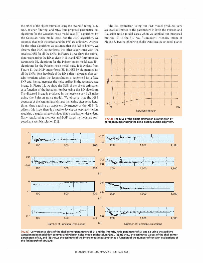
the MSEs of the object estimates using the inverse filtering, LLS,NLS, Wiener filtering, and MLG (our proposed parametric MLalgorithm for the Gaussian noise model case [9]) algorithms forthe Gaussian noise model case. For the MLG algorithm, weassumed that both the object and the PSF are unknown, whereasfor the other algorithms we assumed that the PSF is known. Weobserve that MLG outperforms the other algorithms with thesmallest MSE for all the SNRs. In Figure 11, we show the estima-tion results using the BD as given in (11) and MLP (our proposedparametric ML algorithm for the Poisson noise model case [9])algorithms for the Poisson noise model case. It is evident fromFigure 11 that MLP outperforms BD in MSE by big margins forall the SNRs. One drawback of the BD is that it diverges after cer-tain iterations when the deconvolution is performed for a fixedSNR and, hence, increases the noise artifact in the reconstructedimage. In Figure 12, we show the MSE of the object estimationas a function of the iteration number using the BD algorithm.The distorted image is produced in the presence of 40 dB noiseusing the Poisson noise model. We observe that the MSEdecreases at the beginning and starts increasing after some itera-tions, thus causing an apparent divergence of the MSE. Toaddress this issue, there is a need to develop a stopping criterion,requiring a regularizing technique that is application-dependent.Many regularizing methods and MAP-based methods are pro-posed as a possible solution [11].

The ML estimation using our PSF model produces veryaccurate estimates of the parameters in both the Poisson andGaussian noise model cases when we applied our proposedmethod [9] to the 3-D real fluorescent intensity image of Figure 8. Two neighboring shells were located on focal planes

[FIG12] The MSE of the object estimation as a function ofiteration number using the blind deconvolution algorithm.

240

80

MS

E0 100

×10−4

Iteration Number

[FIG13] Convergence plots of the shell center parameters of S1 and the intensity ratio parameter of S1 and S2 using the additiveGaussian noise model (left column) and Poisson noise model (right column): (a), (b), (c) show the estimated values of the shell centerparameters of S1, and (d) shows the estimate of the intensity ratio parameter as a function of the number of function-evaluations ofthe fminsearch of MATLAB.

100 500

(a)

−1

−2

100 500 900

(c)

0

−1

100 500 900

(d)Number of Function Evaluations

1

0.7

200 1,000 1,800

−1.2

−1.8

200 1,000 1,800

−0.2

−0.8

200 1,000 1,800

0.5

−0.5

Number of Function Evaluations

200 1,000 1,800

1

0.8

100 500 900

(b)

−0.2

−0.8

900


from −2.6 µm to 2.6 µm above and below the plane ofreference at 0 µm and in radial planes from −6.4 µm to6.4 µm along both axes. In Figure 13, we present the conver-gence plots of the ML estimates of the shell center parame-ters of S1 and the intensity ratio parameter of S1 and S2 as afunction of the number offunction-evaluations of thefminsearch of MATLAB for theadditive Gaussian and Poissonnoise models, respectively. (Thefminsearch uses a multidimen-sional unconstrained nonlinearminimization method to mini-mize functionals.) For the addi-tive Gaussian noise model, the convergence plots of the MLestimates did not change appreciably after 350 iterations,whereas for the Poisson noise model the convergence plotsbecame completely steady after 450 iterations. We used anIntel, Pentium-4 CPU, 2-GHz computer with 768 MB of RAMfor performing our simulations. For the Gaussian andPoisson noise models, each function evaluation took 50 and15 s, respectively. The convergence plots using the additiveGaussian noise model are a little bit fuzzy. The Poisson noisemodel demonstrates more stable behavior (see Figures 13)than that of the Gaussian noise model. Therefore, we claimthat the Poisson noise model is more reliable than the addi-tive Gaussian noise model and it provides a better descriptionof the photon-limited image recording of the fluorescencemicroscopy imaging in real life. In our ongoing research,

reliability of the estimation performance is of the utmostimportance and, hence, the computer simulation is quiteintensive. However, we must note that our method extractscertain information of interest from the captured 3-D image,whereas conventional image deconvolution techniques

improve the resolution andSNR of the captured image(see [9] for more details).

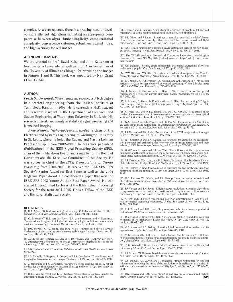
CONCLUSIONSWe have briefly reviewed exist-ing image deconvolution algo-rithms for 3-D fluorescencemicroscopy (see Table 2 for a

summary). It is often recommended that several algorithmsbe applied to the captured image to extract as many specimenfeatures as possible [6]. A limitation of most algorithms is theunderlying assumption of the shift-invariance property of themicroscope system, which is not true in practice. In manyreal situations, some knowledge of the PSF can be obtained.Therefore, a functional modeling of the PSF can be accom-plished with a number of unknown parameters as we proposein [9], resulting in an efficient algorithm. In addition, the per-formance of several iterative algorithms is strongly affected bythe estimation and removal of the background. An overesti-mation of the background compromises the performance ofthe algorithm. Most of the advanced algorithms are nonlinearand statistical, and their implementation for routine 3-Ddeconvolution of microscopy images is computationally

TYPE METHOD REFERENCES NOISE MODEL COMMENTS1) NO-NEIGHBORS [6], [15] NOT ASSUMED SIMPLE AND FAST; REDUCE SNR AND INTRODUCE2) NEIGHBORING NEAREST-NEIGHBORS METHODS [1] STRUCTURAL ARTIFACTS IN THE RESTORED

MULTI-NEIGHBORS METHODS IMAGE.3) LINEAR INVERSE FILTERING [6] NOT ASSUMED SIMPLE AND FAST; AMPLIFY NOISE; INTRODUCE

WIENER FILTERING [16]–[17] ADDITIVE GAUSSIAN RINGING ARTIFACTS AND SUPPRESS HIGHLLS [18] FREQUENCY COMPONENTS IN THE RESTOREDTIKHONOV FILTERING [5] IMAGE.

4) NONLINEAR, JVC [1] NOT ASSUMED ENFORCE NONNEGATIVITY CONSTRAINT INITERATIVE NLS [18]–[19] NOT ASSUMED AN AD HOC MANNER; INCREASE RESOLUTION

IN THE ESTIMATED IMAGE BUT NOT EFFICIENTIN REMOVING NOISE.

ICTM [4], [8], [20], ADDITIVE GAUSSIAN INCREASE COMPUTATION; DECONVOLUTION[21] RESULT DEPENDS ON REGULARIZATION PARA-

METER AND REGULARIZATION MATRIX.CARRINGTON [4], [20], [21]

5) STATISTICAL, ML/EM [11], [23]–[25] POISSON RESTORE HIGH NOISE LEVEL; EM HAS SLOWITERATIVE RATE OF CONVERGENCE; ML CONVERGES TO

NOISE ASYMPTOTICALLY, REQUIRING REGULARIZATION AT THE COST OF INCREASED COMPUTATIONAL LOAD.

PARAMETRIC ML [9] ADDITIVE GAUSSIAN, APPLICABLE WHEN BOTH THE SPECIMEN ANDPOISSON PSF ARE IN PARAMETRIC FORM.

GAUSSIAN OR ENTROPY PRIOR DISTRIBUTIONOF THE OBJECT IS ASSUMED AND HENCEGIVES BETTER PERFORMANCE; EMPLOY

MAP [26]–[28] ADDITIVE GAUSSIAN, REGULARIZATION AND THE CHOICE OF POISSON REGULARIZATION PARAMETER DETERMINES THE

TRADE-OFF BETWEEN AMOUNT OF SMOOTHNESSAND FITTING ACCURACY.

6) BLIND BD/RL [7], [24], POISSON LARGE NUMBER OF PARAMETERS ARE INVOLVED,DECONVOLUTION [29]–[33] HENCE COMPUTATIONALLY INTENSIVE.

[TABLE 2] GENERAL CHARACTERISTICS OF DECONVOLUTION METHODS OF 3-D FLUORESCENCE MICROSCOPY IMAGES.

IMAGING SYSTEMS ALWAYSDISTORT OBJECTS. IMAGE

DECONVOLUTION RESTORESOBJECTS TYPICALLYBY CHARACTERIZING

THIS DISTORTION.


complex. As a consequence, there is a pressing need to devel-op more efficient algorithms exhibiting an appropriate com-promise between algorithmic simplicity, computationalcomplexity, convergence criterion, robustness against noise,and high accuracy for real images.

ACKNOWLEDGMENTSWe are grateful to Prof. David Kelso and John Ketterson ofNorthwestern University, as well as Prof. Alan Feinerman ofthe University of Illinois at Chicago, for providing the imagesin Figures 1 and 8. This work was supported by NSF GrantCCR-0330342.

AUTHORPinaki Sarder ([email protected]) received a B.Tech degreein electrical engineering from the Indian Institute ofTechnology, Kanpur, in 2003. He is currently a Ph.D. studentand research assistant in the Department of Electrical andSystem Engineering at Washington University in St. Louis. Hisresearch interests are mainly in statistical signal processing andbiomedical imaging.

Arye Nehorai ([email protected]) is chair of theElectrical and Systems Engineering of Washington Universityin St. Louis, where he holds the Eugene and Martha LohmanProfessorship. From 2002–2005, he was vice president(Publications) of the IEEE Signal Processing Society (SPS),chair of the Publications Board, and a member of the Board ofGovernors and the Executive Committee of this Society. Hewas editor-in-chief of the IEEE Transactions on SignalProcessing from 2000–2002. He received the IEEE SPS 1989Society’s Senior Award for Best Paper as well as the 2004Magazine Paper Award. He coauthored a paper that won theIEEE SPS 2003 Young Author Best Paper Award. He waselected Distinguished Lecturer of the IEEE Signal ProcessingSociety for the term 2004–2005. He is a Fellow of the IEEEand the Royal Statistical Society.

REFERENCES[1] D.A. Agard, “Optical sectioning microscopy: Cellular architecture in threedimensions,” Ann. Rev. Biophys. Bioeng., vol. 13, pp. 191–219, 1984.

[2] G. Brakenhoff, H.T. van der Voort, E.A. van Spronson, and N. Nanninga, “3-dimensional imaging of biological structures by high resolution confocal scan-ning laser microscopy,” Scanning Microsc., vol. 2, no. 1, pp. 33–40, 1988.

[3] P.W. Stevens, C.H.J. Wang, and D.M. Kelso, “Immobilized particle arrays:Coalescence of planar and suspension-array technologies,” Analyt. Chem., vol. 75,no. 5, pp. 1141–1146, 2003.

[4] G.M.P. van der Kempen, L.J. van Vliet, P.J. Verveer, and H.T.M. van der Voort, “A quantitative comparison of image restoration methods for confocalmicroscopy,” J. Microsc., vol. 185, no. 3, pp. 354–365, 1997.

[5] A.N. Tikhonov and V.Y. Arsenin, Solutions of Ill-Posed Problems. Wiley: NewYork, 1977.

[6] J.G. McNally, T. Karpova, J. Cooper, and J.A. Conchello, “Three-dimensionalimaging by deconvolution microscopy,” Methods, vol. 19, no. 3, pp. 373–385, 1999.

[7] J. Markham and J. Conchello, “Parametric blind deconvolution: A robustmethod for the simultaneous estimation of image and blur,” J. Opt. Soc. Amer. A.,vol. 16, no. 10, pp. 2377–2391, 1999.

[8] H.T.M. van der Voort and K.C. Strasters, “Restoration of confocal images forquantitative image analysis,” J. Microsc., vol. 178, no. 2, pp. 165–181, 1995.

[9] P. Sarder and A. Nehorai, “Quantifying fluorescence of quantum dot encodedmicroparticles using maximum likelihood estimation,” to be published.

[10] S.F. Gibson and F. Lanni, “Experimental test of an analytical model of aberra-tion in an oil-immersion objective lens used in three-dimensional lightmicroscopy,” J. Opt. Soc. Amer. A., vol. 8, no. 10, pp. 1601–1612, 1991.

[11] T.J. Holmes, “Maximum-likelihood image restoration adapted for non coher-ent optical imaging,” J. Opt. Soc. Amer. A., vol. 5, no. 5, pp. 666–673, 1988.

[12] The XCOSM package, Biomedical Computer Laboratory, WashingtonUniversity, St. Louis, MO, May 2002 [Online]. Available: http://rayleigh.omrf.ouhsc.edu/~xcosm/

[13] V.N. Mahajan, “Zernike circle polynomials and optical aberrations of systemswith circular pupils,” Eng. Lab. Notes, vol. 17, pp. S21–S24, 1994.

[14] W.Y. Kim and Y.S. Kim, “A regino based-shape descriptor using Zernikemoments,” Signal Processing: Image Commun., vol. 16, no. 1, pp. 95–102, 2000.

[15] J.R. Monck, A.F. Oberhauser, T.J. Keating, and J.M. Fernandez, “Thin-sectionratiometric Ca2+ images obtained by optical sectioning of fura-2 loaded mastcells,” J. Cell Biol., vol. 116, no. 3, pp. 745–759, 1992.

[16] T. Tomasi, A. Diaspro, and B. Bianco, “3-D reconstruction in opticalmicroscopy by a frequency-domain approach,” Signal Processing, vol. 32, no. 3, pp.357–366, 1993.

[17] A. Erhardt, G. Zinser, D. Komitowski, and J. Bille, “Reconstructing 3-D light-microscopic images by digital image processing,” Applied Opt., vol. 24, no. 2, pp. 194–200, 1985.

[18] C. Preza, M.I. Miller, L.J. Thomas Jr., and J.G. McNally, “Regularized linearmethod for reconstruction of three-dimensional microscopic objects from opticalsections,” J. Opt. Soc. Amer. A., vol. 9, pp. 219–228, 1992.

[19] W.A. Carrington, K.E. Fogarty, and F.S. Fay, “3D fluorescence imaging of sin-gle cells using image restoration,” in Noninvasive Techniques in Cell Biology, K.Foskett and S. Grinstein, Eds. New York: Wiley-Liss, 1990, pp. 53–72.

[20] P.J. Verveer and T.M. Jovin, “Acceleration of the ICTM image restoration algo-rithm,” J. Microsc., vol. 188, pp. 191–195, 1997.

[21] N.P. Galatsanos and A.K. Katsaggelos, “Methods for choosing the regulariza-tion parameter and estimating the noise variance in image restoration and theirrelation,” IEEE Trans. Image Processing, vol. 1, no. 3, pp. 322–336, 1992.

[22] G.M.P. van Kempen and L.J. van Vliet, “The influence of the regularizationparameter and the first estimate on the performance of Tikhonov regularized non-linear image restoration algorithms,” J. Microsc., vol. 198, no. 1, pp. 63–75, 2000.

[23] A.P. Dempster, N.M. Laird, and D.B. Rubin, “Maximum likelihood from incom-plete data via the EM algorithm,” J. R. Statist. Soc. B, vol. 39, no. 1, pp. 1–38, 1977.

[24] T.J. Holmes, “Blind deconvolution of quantum-limited incoherent imagery:Maximum-likelihood approach,” J. Opt. Soc. Amer. A, vol. 9, no. 7, pp. 1052–1061,1992.

[25] R.G. Paxman, T.J. Schulz, and J.R. Fienup, “Joint estimation of object andaberrations by using phase diversity,” J. Opt. Soc. Amer. A., vol. 9, no. 7, pp.1072–1085, 1992.

[26] P.J. Verveer and T.M. Jovin, “Efficient super resolution restoration algorithmsusing maximum a posteriori estimations with application to fluorescencemicroscopy,” J. Opt. Soc. Amer. A., vol. 14, no. 8, pp. 1696–1706, 1997.

[27] S. Joshi and M.I. Miller, “Maximum a posteriori estimation with Good’s rough-ness for optical sectioning microscopy,” J. Opt. Soc. Amer. A., vol. 10, no. 5, pp.1078–1085, 1993.

[28] H.J. Trussell and B.R. Hunt, “Improved methods of maximum a posteriorirestoration,” IEEE Trans. Comput., vol. 27, pp. 57–62, 1979.

[29] D.A. Fish, A.M. Brinicombe, E.R. Pike, and J.G. Walker, “Blind deconvolutionby means of the Richardson-Lucky algorithm,” J. Opt. Soc. Amer. A., vol. 12, no. 1, pp. 58–65, 1995.

[30] G.R. Ayers and J.C. Dainty, “Iterative blind deconvolution method and itsapplications.,” Optics Lett., vol. 13, no. 7, pp. 547–549, 1988.

[31] V. Krishnamurthi, Y.H. Liu, S. Bhattacharyya, J.N. Turner, and T.J. Holmes,“Blind deconvolution of fluorescence micrographs by maximum-likelihood estima-tion,” Applied Opt., vol. 34, no. 29, pp. 6633–6647, 1995.

[32] G.B. Avinash, “Simultaneous blur and image restoration in 3D opticalmicroscopy,” Zool. Stud., vol. 34, no. 1, pp. 185–185, 1995.

[33] T.J. Schulz, “Multi-frame blind deconvolution of astronomical images,” J. Opt.Soc. Amer. A., vol. 10, no. 5, pp. 1064–1073, 1993.

[34] J.B. Monvel, S.L. Calvez, and M. Ulfendahl, “Image restoration for confocalmicroscopy: Improving the limits of deconvolution, with application to the visuali-zation of the mammalian hearing organ,” Biophys J., vol. 80, no. 5, pp. 2455–2470,2001.

[35] P.W. Stevens and D.M. Kelso, “Imaging and analysis of immobilized particlearrays,” Analyt. Chem., vol. 75, no. 5, pp. 1147–1154, 2003. [SP]

Documents

Deconvolution Methods for 3-D Fluorescence Microscopy …