Deep Generative Models of Urban Mobility

Ziheng Lin∗

Civil Systems, CEE, UC Berkeleyzihenglin@berkeley.edu

Mogeng Yin†

Transportation, CEE, UC Berkeleymogengyin@berkeley.edu

Sidney Feygin‡

Civil Systems, CEE, UC Berkeleysid.feygin@berkeley.edu

Madeleine SheehanTransportation, CEE, UC Berkeley

Jean-Francois PaiementAT&T Research

Alexei PozdnoukhovCEE, UC Berkeley

ABSTRACTLocational data generated by mobile devices present an opportu-nity to substantially simplify methodologies and reduce analysislatencies in transportation planning applications. In this paper,we describe a modeling framework that supports most commontransportation planning tasks, delivering actionable solutions at afraction of time and cost as compared to the state of practice. �eframework builds up on cell phone data processing and activity-based inferences of travel purposes with an Input-Output HiddenMarkov Model (IO-HMM), followed by a Long Short Term Memory(LSTM) network that learns travelers’ mobility sequences. It com-bines the desired interpretability due to the parametric speci�cationof an IO-HMM with �exibility and predictive power of deep neuralmodels. We describe our target use case for the synthesized activitychains: delivering decision support and transportation scenarioevaluation to practitioners. We outline domain-driven operationalobjectives and verify that our framework meets these criteria byillustrating its usability in typical transportation demand planningapplications. It is currently being deployed for testing by a majornetwork carrier serving millions of users in the San Francisco BayArea.

CCS CONCEPTS•Computing methodologies →Modeling methodologies;

KEYWORDSCellular data, generative models, recurrent neural network, demandforecasting, activity-based models

ACM Reference format:Ziheng Lin, Mogeng Yin, Sidney Feygin, Madeleine Sheehan, Jean-FrancoisPaiement, and Alexei Pozdnoukhov. 2017. Deep Generative Models of UrbanMobility. In Proceedings of ACM SIGKDD Conference, Halifax, Nova Scotia,Canada, August 13-17, 2017 (KDD’17), 9 pages.DOI: 10.475/123 4

∗equally contributing author†equally contributing author‡equally contributing author

Permission to make digital or hard copies of part or all of this work for personal orclassroom use is granted without fee provided that copies are not made or distributedfor pro�t or commercial advantage and that copies bear this notice and the full citationon the �rst page. Copyrights for third-party components of this work must be honored.For all other uses, contact the owner/author(s).KDD’17, Halifax, Nova Scotia, Canada© 2017 Copyright held by the owner/author(s). 123-4567-24-567/08/06. . .$15.00DOI: 10.475/123 4

1 INTRODUCTIONFrom the exponential growth of on-demand shared ride serviceslike Uber and Ly� to an increased reliance on public transit in theface of environmental concerns over emissions and uncertainty ingas prices, today’s transportation policy makers and planners mustdeal with a rapidly changing urban mobility landscape. Despitemethodological and technical advances in survey distribution andprocessing over the last 20 years [1], improvements in the accuracyof transportation demand prediction models have remained �at [15].As a consequence, project overruns due to inaccurate economicvalue appraisals continue to cost taxpayers billions of dollars [9, 34].Non-invasive, automated, continuous data collection mechanismsare increasingly being used to complement manual survey tech-niques by improving their statistical representativeness [12]. Inparticular, large volumes of call detail records (CDRs) from mobilephones have been used to construct individual daily itinerariesand train travel activity models using weeks and months of datarather than several days’ worth [36]. While applications of miningmobility trajectories from crowd-sourced locational data are com-mon (these are thoroughly reviewed in Section 2), existing modelso�en trade o� the interpretability that transportation practitionersrequire in practice for the computational tractability necessary todeal with large volumes of data [10].

In practice, the activity-based travel models used by practitionersare incredibly rich in describing the intricacies of human activitiesand context of decision making in travel-related choices. �e ap-peal of econometric models estimated from these stated preferencedata of transportation system users rests on empirically-validatedutility maximization axioms and the estimation of parameters forlinear models that explain choices based on the characteristics ofindividual decision makers and the a�ributes of the alternativesunder consideration [4]. One key research challenge for the ma-chine learning community in this domain thus lies in developinga framework that reduces reliance on domain experts to specifyrobust models of travel decision-making while maintaining the�exibility to include covariates that rationalize observed behaviorand responses to the applied system-level policies.

1.1 Contribution of this workIn this paper, we describe the developed two-step generative mod-eling framework that is capable of learning activity sequences fromlarge volumes of call data while incorporating behavioral param-eters that are sensitive to policy levers. By combining recurrentneural networks with probabilistic modeling techniques speci�c tothe task of generating human activity chains from cellular data, we

KDD’17, August 13-17, 2017, Halifax, Nova Scotia, Canada Z. Lin et al.

thus expand the scope of state-of-the-art human mobility model-ing techniques to the realm of decision support for transportationpolicy analysis.

�is paper details the following contributions:• We implement an extensible end-to-end processing and in-

ference pipeline: using raw cellular data as input, our dataprocessing framework provides transportation planners,policy-makers and related stakeholders with detailed andtimely travel demand models.

• To the best of the authors’ knowledge, this is the �rstwork using deep recurrent neural network architecture togenerate human activity chains from cellular data. �anksto its �exibility in modeling long temporal dependenciesand explicit location choices, it was found to be the keymodeling component to be deployed in practice.

• Leveraging rich activity-based inferences of observed travel,we connect our framework with the state-of-the-art dis-crete choice modeling to include socio-economic variablesinto explicit choice models that inform scenario micro-simulation and support policy evaluation by practitioners.

To validate the framework, we sample trained generative models toproduce synthetic travel plans for the population in the region, anduse them as inputs to an agent-based microscopic tra�c simulator.We validate the resulting tra�c volumes against an independentdataset of tra�c counts collected on all the major freeways andtransit lines within the region of study.

As the framework is currently being implemented for a test de-ployment in the San Francisco Bay Area, we discuss some additionalmetrics that we have set to validate its usability in practice.

2 RELATEDWORKEnabled by petabyte-scale data processing techniques, urban com-puting innovations and challenges have been drawing increasingsocial, commercial, and academic a�ention in the past decade [40].Human activity recognition from spatiotemporal microdata streams,an application of urban computing research, has been explored ex-tensively by practitioners across disciplines[10, 16]. A summary ofrelevant developments in urban activity modelling is given belowwith respect to the main data sources and the properties of theexplored algorithms.

2.1 Locational Data SourcesGPS data is granular in both spatial and temporal resolution. Earlywork in extracting signi�cant places took advantage of this rela-tively rich data source for activity inference models [24, 41]. How-ever, collecting GPS data o�en requires active user participation andpermissions for physical devices as well as careful ba�ery manage-ment, thus limiting its practicality in terms of collecting continuousand representative samples from traveler populations.

Locational-based social network (LBSN) data usually containslocations of users of a service at the time of interaction (a check-in), and is limited by the frequency of users’ check-ins. Basedon LBSN data, researches have developed methods for classifyingactivities into distinct categories [23, 37], for separating social tripsfrom commute trips [11], promoting products and services [42] andinferring mobility of grouped individuals [39].

LSTM Sequence Modeling

TransportSimulation

IO-HMM Activity Recognition

Data Key Components Product

k-anonymity and DP

filterCDR

Activity Sequences

Activity Recognition with IO-HMM

SyntheticTravelPlans

Traffic and

TransitData

MicroscopicSimulator

Traffic Simulation

and Validation

Stored data Database Process Derived Data Outputs

LSTM Training

LSTM Models

Activity Labels

Privacy Test and Filter

Travel Demand

Explorer

Discrete Choice

Modeler

Census Data

Figure 1: Modeling framework diagram.

�e anonymized Call Detail Records (CDRs) from cellular net-work operators provide a compromise between spatial-temporalresolution and ubiquity. Due to its relatively poor resolution inspace, CDR data has been mainly used to derive spatially aggre-gated results such as mass movements of population [13], aggre-gated origin-destination (OD) estimation [35], stylized mobilitylaws [16, 29], and disaster response [25]. Until recently, there waslimited work using cellular data for urban activity recognition [36],especially in the context of high-�delity travel modelling [38].

2.2 Generative Models for Sequential DataTo a large extent, human mobility is structured by highly regulardaily/weekly schedules, demonstrating high predictability acrossdiverse populations [16]. Longitudinal analysis also suggests thathuman mobility has high temporal and spatial regularities [29].With the right tools, these pa�erns can be employed in predictivemodels.

Recurrent neural networks (RNNs) have become the state ofthe art for sequence modeling and generation, especially in thelanguage and translation domain [31]. Long short term memory(LSTM) [21] is one of the most popular variations of RNNs withproven ability to generate sequences in various domains, such astext [30], images [18] and hand-writing [17]. A recent work showedthe capability of LSTM to predict pedestrians’ motion from videodata [2]. �e success of RNNs in these domains motivated ourwork of applying RNNs for human activity sequence modeling andgeneration.

Hidden (semi-) Markov models are generative models that cannot only be used to analyze activity pa�erns, but also to generatenew sequences [19]. Our recent work used Input-Output HiddenMarkov Models (IO-HMMs) to reveal urban activity pa�erns (in-cluding the spatial-temporal pro�les of urban activity and hetero-geneous transition probabilities) and to generate synthetic activitysequences to inform microscopic tra�c simulations [38].

�e advantages of IO-HMM over standard HMM is that it relaxesthe assumption that the transition probabilities and emission proba-bilities are homogeneous. Instead, the transitions and emissions inIO-HMM can depend on the contextual variables such as time of dayand day of week. While HMMs bene�t from a simple interpretablestructure and an ability to model dynamic latent variables, theysu�er from a few limitations. For one, when training the model, the

Deep Generative Models of Urban Mobility KDD’17, August 13-17, 2017, Halifax, Nova Scotia, Canada

ActivityFeatures

IO-HMMActivityInference

CDR Trace

f1 f2 f3 f4 f5

HWO

HWO

HWO

HWO

HWO

GenerativeLSTMTraining

SyntheticSequences

Figure 2: Processing of a CDR trace to synthetic activitysequence, featuring aHome-Work-Other-Work-Home activ-ity chain. Raw CDR traces are �rst converted to spatial, tem-poral and contextual activity features. IO-HMMs are used toidentify activity labels. Activity sequences with labels aresent to LSTM recurrent generative neural networks.

number of hidden nodes (each hidden node corresponds to an activ-ity) needs to be pre-speci�ed. Although one can use the number ofconventional urban activities (home, work, food, shop, recreation,etc.), the learned activities do not necessarily correspond to eachpre-de�ned activity type.

LSTMs, on the other hand, are more �exible as they use manycontinuous hidden units with implicit embedding corresponds tothe discrete activities. LSTM also holds an advantage over HMMsin modeling long term dependencies thanks to the automaticallylearned “input”, “output” and “forget” gates. Moreover, the �ex-ibility and the tremendous learning power allows LSTMs to pa-rametrize complex joint distributions required to reproduce thevariability of destination location choice for urban travelers withheterogeneous preferences and lifestyles.

3 MODELING FRAMEWORKIn our previous work, we have used IO-HMMs to recognize urbanactivity, analyze activity pa�erns, and generate synthetic activitychains [38]. �e activity recognition resulted an accuracy of 88%for home, work and all secondary activities. However, one missingpiece in the work is explicit and privacy preserving location choicesof activities. A common approach is to sample a random locationwithin a tra�c analysis zone (TAZ), which is chosen based onthe learned spatial coe�cients (distance to home and distance towork) of the activity. In this work, we are interested in an activitysequence modeling framework for producing realistic syntheticactivity plans including explicit location choices, while preservingthe interpretability of the IO-HMM model. �is objective leads usto the following two-step framework of generating urban activities.

(1) In the �rst step, raw CDR data containing a timestampedrecord for each communication of anonymous user’s deviceserved by the cellular network go through a k-anonymitycheck [32] and optional di�erential privacy (DP) �lters [20,27] as required by a data provider. �e masked CDR data

are then pre-processed to a sequence of stay location clus-ters that may correspond to distinct yet unlabeled activities.A�ributes of each activity, such as the start time, duration,location features, and the context of the activity (whetherthis activity happens during a home-based trip, work-basedtrip, or a commute trip), is also extracted as a result of thisprocessing. IO-HMMs are then used to label each activityand uncover the activity pa�erns [38].

(2) In the second step, the activity sequences, together with therecognized activity labels, are sent to a generative recurrentneural network with LSTM cells for training. �e trainedmodel is able to learn explicit location choice with mixturedensity outputs for each type of activity, and thus capableof generating realistic activity chains. LSTM is designedwith a locational privacy bound parameter that controlsthe variance of sampled locations, making it suitable forplacing additional privacy �lters [7, 20].

�e full framework (shown in Figure 1) has some additionalimportant components. Current practice of understanding trav-eler’s mode choice preference is based on travel surveys that areusually outdated to re�ect the rapid changes in people’s behavior.A discrete choice modeler (DCM) allows us to obtain up-to-datetravelers’ preference using CDR data. Its importance is two-fold: (1)�e calibrated DCM is one of the direct outputs to transportationdecision makers, which can be used for scenario evaluation andurban planning. (2) It is a way to calibrate the utility functions ofagents in a microscopic travel simulation. For enhanced realism inextrapolating scenarios towards unseen situations, we use a simu-lation where agents are independent decision makers with logic oftravel choices (such as travel mode choice given the trip purpose)being governed by a parametric utility function. To this extent wealso use social-demographic information from census data (suchas the median income in the district a traveler lives) as contextualvariables to make the discrete choice model more accurate andpractical in extrapolating scenarios [4], as detailed in Section 5.3.

Finally, travel plans are generated for the synthetic population inthe region from the generative LSTM model. Synthetic travel plansdo not correspond to any real user trajectories. To further protectprivacy, traces that are too close to real trajectories can be �lteredusing existing techniques [7, 20]. �e �ltered synthetic travel plans,together with the travelers’ travel mode choice parameters, are fedto a microscopic transport simulator.

�e output of the simulator provides:

• detailed daily travel itineraries of the synthetic population,• tra�c volumes and transit passenger counts for compari-

son against real counts from highway sensors and transitagencies data,

• range of metrics for a given scenario including its environ-mental impact,

• aggregated travel demand volumes and performance met-rics accessible through basic interactive elements imple-mented within the travel demand explorer (Figure 9) toevaluate the proposed policy and infrastructure changesin the transportation system.

KDD’17, August 13-17, 2017, Halifax, Nova Scotia, Canada Z. Lin et al.

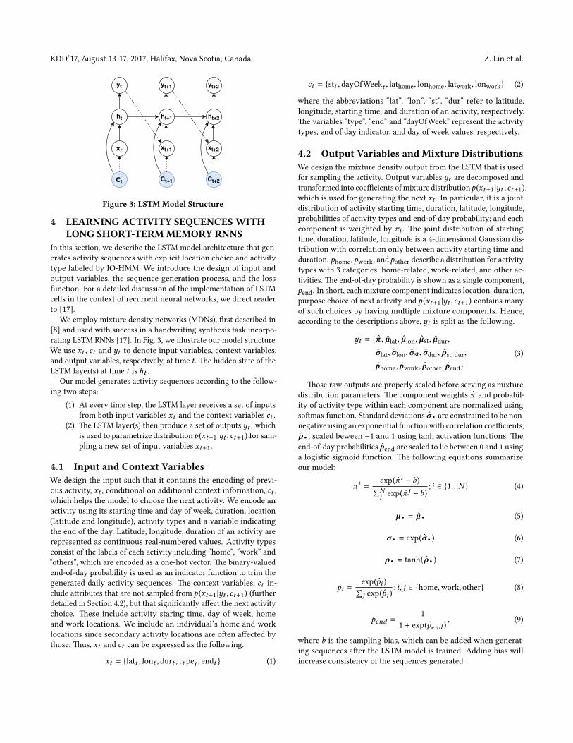
Figure 3: LSTM Model Structure

4 LEARNING ACTIVITY SEQUENCES WITHLONG SHORT-TERMMEMORY RNNS

In this section, we describe the LSTM model architecture that gen-erates activity sequences with explicit location choice and activitytype labeled by IO-HMM. We introduce the design of input andoutput variables, the sequence generation process, and the lossfunction. For a detailed discussion of the implementation of LSTMcells in the context of recurrent neural networks, we direct readerto [17].

We employ mixture density networks (MDNs), �rst described in[8] and used with success in a handwriting synthesis task incorpo-rating LSTM RNNs [17]. In Fig. 3, we illustrate our model structure.We use xt , ct and yt to denote input variables, context variables,and output variables, respectively, at time t . �e hidden state of theLSTM layer(s) at time t is ht .

Our model generates activity sequences according to the follow-ing two steps:

(1) At every time step, the LSTM layer receives a set of inputsfrom both input variables xt and the context variables ct .

(2) �e LSTM layer(s) then produce a set of outputs yt , whichis used to parametrize distributionp (xt+1 |yt , ct+1) for sam-pling a new set of input variables xt+1.

4.1 Input and Context VariablesWe design the input such that it contains the encoding of previ-ous activity, xt , conditional on additional context information, ct ,which helps the model to choose the next activity. We encode anactivity using its starting time and day of week, duration, location(latitude and longitude), activity types and a variable indicatingthe end of the day. Latitude, longitude, duration of an activity arerepresented as continuous real-numbered values. Activity typesconsist of the labels of each activity including “home”, “work” and“others”, which are encoded as a one-hot vector. �e binary-valuedend-of-day probability is used as an indicator function to trim thegenerated daily activity sequences. �e context variables, ct in-clude a�ributes that are not sampled from p (xt+1 |yt , ct+1) (furtherdetailed in Section 4.2), but that signi�cantly a�ect the next activitychoice. �ese include activity staring time, day of week, homeand work locations. We include an individual’s home and worklocations since secondary activity locations are o�en a�ected bythose. �us, xt and ct can be expressed as the following.

xt = {latt , lont , durt , typet , endt } (1)

ct = {stt , dayOfWeekt , lathome, lonhome, latwork, lonwork} (2)

where the abbreviations “lat”, “lon”, “st”, “dur” refer to latitude,longitude, starting time, and duration of an activity, respectively.�e variables “type”, “end” and “dayOfWeek” represent the activitytypes, end of day indicator, and day of week values, respectively.

4.2 Output Variables and Mixture DistributionsWe design the mixture density output from the LSTM that is usedfor sampling the activity. Output variables yt are decomposed andtransformed into coe�cients of mixture distributionp (xt+1 |yt , ct+1),which is used for generating the next xt . In particular, it is a jointdistribution of activity starting time, duration, latitude, longitude,probabilities of activity types and end-of-day probability; and eachcomponent is weighted by πi . �e joint distribution of startingtime, duration, latitude, longitude is a 4-dimensional Gaussian dis-tribution with correlation only between activity starting time andduration. phome, pwork, andpother describe a distribution for activitytypes with 3 categories: home-related, work-related, and other ac-tivities. �e end-of-day probability is shown as a single component,pend. In short, each mixture component indicates location, duration,purpose choice of next activity and p (xt+1 |yt , ct+1) contains manyof such choices by having multiple mixture components. Hence,according to the descriptions above, yt is split as the following.

yt = {π , µlat, µlon, µst, µdur,

σlat, σlon, σst, σdur, ρst, dur,

phome, pwork, pother, pend}

(3)

�ose raw outputs are properly scaled before serving as mixturedistribution parameters. �e component weights π and probabil-ity of activity type within each component are normalized usingso�max function. Standard deviations σ· are constrained to be non-negative using an exponential function with correlation coe�cients,ρ· , scaled beween −1 and 1 using tanh activation functions. �eend-of-day probabilities pend are scaled to lie between 0 and 1 usinga logistic sigmoid function. �e following equations summarizeour model:

π i =exp(π i − b)∑Nj exp(π j − b)

; i ∈ {1...N } (4)

µ· = µ· (5)

σ· = exp(σ· ) (6)

ρ· = tanh(ρ· ) (7)

pi =exp(pi )∑j exp(pj )

; i, j ∈ {home,work, other} (8)

pend =1

1 + exp(pend ), (9)

where b is the sampling bias, which can be added when generat-ing sequences a�er the LSTM model is trained. Adding bias willincrease consistency of the sequences generated.

Deep Generative Models of Urban Mobility KDD’17, August 13-17, 2017, Halifax, Nova Scotia, Canada

Now, we write mixture of joint distribution as follows.

p (xt |yt−1, ct ) =N∑iπ ipi (xt |yt−1, ct )

N∑iπ ipi (latt , lont , stt , durt , typet , endt |yt−1, ct )

(10)

We de�ne the following decomposition of the joint distribution sothat the loss (negative log-likelihood) of the model can be calculatedconveniently.

pi (latt , lont , stt ,durt , typet , endt |yt−1, ct )def= pi (latt , lont )·

pi (stt , durt ) · pi (typet ) · pi (endt )(11)

pi (latt , lont ) = N *,latt , lont

������

[µilatµilon

], Σilat, lon

+-

(12)

pi (stt , durt ) = N *,stt , durt

������

[µistµidur

], Σist,dur

+-

(13)

pi (typet ) =∑jjt ·pj + (1 − jt ) · (1 − pj );

j ∈ {home,work, others}jt ∈ {0, 1}

(14)

pi (endt ) = endt · pend + (1 − endt ) · (1 − pend) (15)Here we split a single spatiotemporal four-dimensional Gaussiandistribution into two two-dimensional Gaussian distributions forbe�er computation e�ciency, with an assumption of independencebetween the spatial (latitude, longitude) and temporal variables.

4.3 Sequence generationSequence generation is initialized by feeding the LSTM model withx0 and c0. We specify the initial input vector x0 as constant since wedo not give the model any information about the �rst activity andthe model should generate the �rst activity from its learnt weights.�e initialization of c0 is described in Section 5.2. Starting fromt = 1, we sample location, duration, activity type and end-of-dayprobability from p (xt |yt−1, ct ), which is a mixture distribution con-ditional on the observed starting time of the activity. �e mixtureweights are calculated as the following.

wi (stt ) =π i · N (stt |µst,σst)i∑Nj π j · N (stt |µst,σst) j

(16)

Because of the correlation between activity staring time andduration, the mean and standard deviation of activity durationconditioned on the observed starting time, stt , is expressed as

µdur |stt = µdur +σdurσst· ρst,dur · (stt − µst) (17)

σdur |stt =√(1 − ρ2

st,dur) · σdur (18)

Now we can sample a new activity xt from the mixture dis-tribution p (xt |yt−1, ct ) following Eq. 19 through Eq. 23. First, acomponent is sampled from the multinomial distribution of mix-ture weights ( Eq. 16). �en, durt , latt , lont , typet , endt can be

further sampled from the selected component, yielding a joint dis-tribution of all those variables. Once a new activity is sampled, thetime of day in ct is incremented by durt .

k ∼ Multinomial(w (stt )1, ...,w (stt )N ;n = 1

)(19)

latt , lont ∼ N *,

µklatµklon

, Σklat, lon

+-

(20)

durt ∼ N(µkdur |stt ,σ

kdur |stt

)(21)

typet ∼ Multinomial(pkhome,p

kwork,p

kothers;n = 1

)(22)

endt ∼ Binomial(pkend

)(23)

4.4 Loss Function and Model EstimationWe use negative log-likelihood as the loss of the model. �e lossfunction can be decomposed using Eq. 10 through Eq. 15.

loss =T∑t=1− log

N∑iπ ipi (xt |yt−1, ct ) (24)

Given an activity chain, the loss is calculated as sum of negative log-likelihood of each observed activity. �us, it is cumulative over theentire sequence. �e �nal gradients are backpropagated throughthe model weights at each time step. We use the Adam optimizer[22] for the stochastic gradient descent.

Individuals may have di�erent numbers of daily activities suchthat the LSTM model has to handle sequences with di�erent length.Most implementations of LSTM networks do not directly handlesequences with di�erent length because the number of unrollingsteps is �xed when the model is compiled. We use zero padding topad activity sequences to the same length; and the loss due to thepadding is masked when calculating the sequence loss.

5 EXPERIMENTAL RESULTS�is section describes the steps in a full-scale regional experimentwhere we train LSTM model for commuters from each of the 34super-districts in the San Francisco Bay Area, in order to developan actionable mobility model for a typical weekday.

�e data used in these studies comprise a month of anonymizedand aggregated CDR logs collected in Summer 2015 by a majormobile carrier in the US, serving millions of customers in the SanFrancisco Bay Area. No personally identi�able information (PII)was gathered or used for this study. As described previously, CDRraw locations are converted into highly aggregated location featuresbefore any actual modeling takes places.

5.1 Data Pre-processingWe pre-process the data following the steps in [38]. �e homeand work locations are identi�ed during the pre-processing step.We take cell phone users that showed up for more than 21 days amonth at their identi�ed “home” place; showed up for more than 14days a month at their identi�ed “work” place; have home and worknot at the same location. �ese criteria identify regular workingcommuters with a day structure containing both distinct Home andWork.

KDD’17, August 13-17, 2017, Halifax, Nova Scotia, Canada Z. Lin et al.

�e median number of activities is 4.4 per weekday and 4.0 perweekend. �is is consistent with the California Household TravelSurvey, reporting a number of 4 activities per day [1].

Overall, the aggregated statistics of activity labeling by IO-HMMmatch with the travel surveys. �e percentage of US employedperson who go to work on an average weekday is 82.9% [33], thisnumber is 83.7% for IO-HMM labeling. Considering the summarystatistics for people who go to work, we compare the percentage ofpeople who participate in activities at di�erent times of day. �epercentage of people participating in at least one activity beforemorning commute, during morning commute and a�er work is3.1%, 14.8% and 46.3% in the Bay Area Travel Survey [6] and thesenumbers are 2.9%, 15.2% and 43.7% in our labeled data.

5.2 Activity Generation from LSTMOne of our goals is to enable activity based travel demand mod-els that use cellular data to create synthetic agent travel pa�ernswithout compromising the privacy of cell phone users. As such,we test our models’ generative power in the Bay Area context —we simulate 463, 000 agents in the Bay Area (15% sample of thecommuters) and create a day-long activity plan for all agents withanticipated start-times, locations, and durations of all activities inthe day.

As travel pa�erns vary greatly over the region, we trained 34LSTM models, each for a subset of cell phone users residing withineach of the 34 super-districts as de�ned by the San Francisco Met-ropolitan Transportation Commission (MTC). Using standard pro-cedures to �t the population marginals with the census data [14],we sample residents home and work locations to create syntheticcommuters with a predetermined home TAZ and work TAZ. �eprecise home and work locations (lat/lon coordinates) are sampleduniformly within the home and work TAZs.

We use single layer of LSTM with 128 units. Number of outputmixture components, N , is chosen as 80. We use 10% dropoutrate for the LSTM units to prevent over ��ing of the data. �econtext variables c0 are initialized with starting time of �rst activitydrawn from the observations within the super-district with addedGaussian noise and home and work locations are determined asmentioned above. �e sampling bias b is tuned as 2.0 in order toreduce number of outliers in the generated sequences. We also apply�lters on the activity sequences generated to delete unrealistic ones:we �ltered the sequences that don’t end with home activities andthose containing multiple consecutive home or work activities.

We present the temporal characteristics of the generated se-quences in Fig. 4 and Fig. 5. In Fig. 4, we observe a decreasingnumber of work and home activities while there is a slight increasein secondary (other) activities. Fig. 5 shows the joint distributions ofstarting time and duration of each activity type. �e home activitiesstarted around noon are relatively short. Night-time home activitieshave strong correlations between staring time and duration. Workactivities show typical working pa�ern of commuters that somelast the entire day staring in the morning while others last only halfof the day. Secondary (other) activities peak around the morningand a�ernoon commute hour and they usually last within 1.5 hours.Finally, the last activities of the day determined by the LSTM modelis consistent with the pa�ern of night-time home activities. We

Figure 4: Number of activities (labeled per highest posteriorprobability) by their respective start time within a course of5 weekdays.

(a) Home (b) Work (c) Other Activities

Figure 5: Joint distribution plot of duration and start hourof labeled activities.

refer a reader to [38] for a similar but much more detailed analysisof inferred activities.

5.3 Behavioral parameters and DCMWhile providing accurate spatio-temporal representation of travel,the IO-HMM/LSTM component of our framework lacks an impor-tant property: it does not relate the observed choices to socio-demographic characteristics of travelers, nor does it allow implicitforecasting of travel choices beyond previously observed condi-tions (changing tolls, transit fares, or increasing travel delays dueto growing congestion). To provide this capability, we developed anadditional modeling component based on discrete xchoice models(DCMs).

Popularized by a Nobel prize winning economic school of thought[26], DCMs are a de facto standard in practical evaluation of thetravelers’ population response to system parameters and policyinterventions. In practice, planners operate with parametric DCMsto learn traveler’s choice preferences and determine how travelerstrade o� various a�ributes of a given set of travel choice alterna-tives [5]. DCMs are typically �t globally to an entire metropolitanregion, but, if used in combination with the IO-HMM/LSTM com-ponent, DCMs allow for rich, activity and context-dependent travelchoice model.

A common assumption in behavioral modeling is that there existsa utilityU , that person n obtains from choosing a travel alternativei , is a linear form over a�ributes of each travel alternative in thechoice set: Uni = βzni + ϵni , where zni represents a vector ofobserved variables of trip i and traveler n, β is a vector of thecorresponding coe�cients that are interacted with each of theobservable variable, and ϵni represents the utility of unobservablefactors that contribute to travel choices.

Deep Generative Models of Urban Mobility KDD’17, August 13-17, 2017, Halifax, Nova Scotia, Canada

�e probability of traveler n selecting travel alternative i is theprobability that the utility of alternative i is greater than the utilityof all other alternatives. With an assumption that ϵni follows ageneralized extreme value Type I distribution and a traveler is con-sidering J total alternatives with known a�ributes, the probabilityof choosing mode i is given by:

Pni =eβzni∑Jj=1 e

βznj

With a powerful set of techniques to infer travel choices withina context of daily tours described above, the presented frameworkenables estimation of DCMs.

Here we illustrate it on a simple case of a travel mode choicemodel, noting that more sophisticated model speci�cations can beconsidered if required. We selected a subset of several hundredtrans-bay trips with an origin or destination of downtown SanFrancisco, where both driving and public transit alternatives areavailable. For this set of observed trips, we used a discriminativemodel to detect trip mode [28], and queried an in-house routingservice that provides travel times and costs for a set of possibletravel alternatives between the observed origin and destinationzones. Eq. (25) shows a DCM speci�cation that accounts for thetime and cost of travel, a traveler’s anticipated income (the medianincome of the traveler�s home census track is used as a proxy for thetraveler’s income), and unobserved systematic mode preferencescaptured in an o�set term βdr ive (the so-called alternative-speci�cconstant).

Vdr ive =βdr ive + βincome ∗ Income

+ βTT ∗TravelTimedr ive

+ βTC ∗TravelCostdr ive (25)Vpublic transit =βTT ∗TravelTimepublic transit

+ βTC ∗TravelCostpublic transit

�e maximum likelihood estimation of this model resulted inparameters listed in Table 1. �e estimated parameters indicate thatthe utility of a travel option decreases as travel time and travel costincrease; that, all else equal, for trips to and from downtown SanFrancisco, travelers have an a�nity for public transit over driving(likely because driving downtown can be a hassle and parking canbe expensive); that higher income travelers are more likely to drive;and �nally, comparing the travel time and cost coe�cients, travelersvalue their time at a rate of about $30/hour 1. �ese result allowevaluating the response of the city commuters to interventions suchas changing transit fares, improving the level of service (travel timeby transit), and evaluating the price at which travelers will chooseUber over existing public transit options. �e inferred values canalso inform the agents’ logic in the micro-simulation of travel.

5.4 Scenario micro-simulationTra�c micro-simulation is a conventional approach in studying per-formance and evaluating transportation planning and developmentscenarios, including the ones where the travel system conditions arechanged and the response is extrapolated with behavioral models.1�is example results in parameter values within a range of common practice, butit serves as an illustration only. Policy analysis conducted by planning authoritiesinvolves a more thorough and detailed investigation.

Table 1: Discrete choice model parameters for travel mode

Variable Coe� Std. error Z P > |Z|

βdr ive -1.048 0.525 -1.996 0.046βincome 0.0156 0.006 2.557 0.011βTT -1.9495 0.413 -4.72 0.000βTC -0.0653 0.061 -1.071 0.284

Micro-simulation of a typical weekday tra�c is performed usingthe MATSim2 platform [3]. MATSim is a state-of-the-art agentbased multi-modal mobility micro-simulation tool that performsmoe choice and tra�c assignment for the set of agents with pre-de�ned activity plans. It varies departure times and routing of eachagent depending on the congestion generated on the network, inorder to maximize agent’s daily utility, parametrically de�ned withseveral parameters including income, the value of time, and modepreference parameters. �e simulation is run on the SF Bay Areanetwork containing all major transit routes, freeways, primary andsecondary roads (network fragment is visualized in Figure 6).

We have compared the results of the �ows simulated from thegenerated activity sequences with the observed tra�c and transitpassenger volumes, provided by the California DOT PerformanceManagement System (PeMS) and the Metropolitan TransportationCommission respectively. �e simulation is run at 15% of the totalpopulation, and the road capacities as well as total resulting countsare scaled accordingly.

Note that observed tra�c and transit passenger counts are notused for model calibration. �ey are used as independent data toevaluate the validity of the synthetic travel sequences producedwith the LSTM model. Fig. 6 demonstrates examples of the threecharacteristic hourly volume pro�les comparing the modeled andobserved counts on freeways. Figure 7 shows examples of transitpassengers counts entering and exiting 2 major rapid transit sta-tions. Validation results for the full set of sensors are presentedin Fig. 8. Fig. 8a shows a comparison of the volumes for three dis-tinct time periods. Fig. 8b summarizes the validation results over300 freeway and transit sensors in terms of the relative error (%volume) over-/under- estimated by the model as compared to theground truth. One can notice lower accuracy at night and earlymorning hours explained by the fact that the model was developedand applied on a subset of daily commuters and did not include alarge portion of trips performed by unemployed population andpeople working from home, besides multiple other tra�c compo-nents (commercial �eets, taxis, visitors) that are out of scope of themodel. Despite it’s relative simplicity, the model has demonstrateda reasonable accuracy (r2 = 0.76,p < 10−3 in Fig. 8a ) as comparedto the ground truth data.

6 CONCLUSIONS AND FUTUREWORKIn this paper, we presented an end-to-end pipeline of processing,modeling, and simulating urban mobility from cellular data. Weintroduced a two-step generative model framework for learningurban activities and mobility. An IO-HMM model, developed inour previous work, is used for labeling activity types of the pre-processed and anonymized cellular data in San Francisco Bay Area.

2 MATSim code available at h�ps://github.com/matsim-org

KDD’17, August 13-17, 2017, Halifax, Nova Scotia, Canada Z. Lin et al.

Figure 6: A fragment of the multi-modal SF Bay Area net-work with sample tra�c volume detectors and transit sta-tions used for validation. Inset graphs illustrate three sam-ple hourly vehicle volume pro�les for observed (orange) andmodeled (blue) �ows on a typical weekday in June 2015.Sample transit counts histograms are shown in Figure 7.

(a) 16th St. and Mission Station (b) MacArthur Station

Figure 7: Actual and simulated boarding and alightingcounts on 2 major BART stations.

We proposed an LSTM model that is capable of learning explicitlocation choices that is applied on the labeled activity sequences.

Both IO-HMM3 and LSTM4 models are evaluated with eithersurvey or real data collected from the transportation network. �eactivities labeled by IO-HMM were validated by comparing the3 IO-HMM code is available at h�ps://github.com/Mogeng/IO-HMM4 LSTM code is available at h�ps://github.com/zihenglin/LSTM-Mobility-Model

(a) Modeled vs observedvolumes at 8am (black),1pm (red) and 6pm (blue).

(b) Mean relative error (%) of mod-elled vs observed tra�c volumesduring the day.

Figure 8: Micro-simulation validation.

aggregated activity statistics with 2015 travel, which showed highsimilarity to the survey results. To examine the generative power ofthe LSTM model, we synthesized urban mobility plans using trainedmodels. An agent-based micro-simulation of travel with multipletravel modes was run using the synthesized plans. �e vehicletra�c counts and public transit boarding and alighting counts fromthe simulation result were compared with real tra�c and transitdata. A reasonable �t accuracy was observed.

We further demonstrated the capabilities of the framework tocontribute to the transportation planning practice by applying adiscrete choice model on traveler’s mode choice. Travelers’ be-havior can be interpreted from the estimated parameters, and theparameters such as the value of time and mode preferences used inmicro-simulation or in other analysis methodologies of evaluatingscenarios in transportation planning and policy making.

6.1 Travel Demand ExplorerSeveral improvements are planned to further build on the work pre-sented herein. We have prototyped and will evaluate the usabilityof our system with a graphical travel demand explorer dashboard(Figure 9), which provides a system-level visualization of alterna-tive mobility scenarios. It shows aggregated travel volumes androutes as well as basic interactive elements to evaluate the impactsof proposed policies and changes in transportation infrastructureon travel impact and level of service metrics.

With privacy concerns in mind, we will also work on improvingperformance and modeling accuracy by partitioning a populationinto �ner sub-groups (whether socially or spatially) to take advan-tage of parameter sharing between the IO-HMM/LSTM models.Along with conducting performance evaluations and enhancingpractical usability, we plan to study the privacy/utility trade-o�s ofthe overall system.

A range of issues remain where limitations of the current designpresent a challenge. One limitation involves DCM calibration fromindirectly assigned socio-demographic variables based on the aggre-gated values within Census tracts. Other limitations are concernedwith the nature of cellular data and inherent di�culties in the iden-ti�cation of the number of car-pools, on-demand vs. private vehicletrips, and modeling short-range and non-motorized travel to namea few.

Deep Generative Models of Urban Mobility KDD’17, August 13-17, 2017, Halifax, Nova Scotia, Canada

Figure 9: Travel demand explorer interface.

We identify the long-term dependency resolution of RNNs andthe expressiveness of probabilistic modeling techniques as two com-ponents that working in concert have the potential to drive thefuture state of practice in transportation demand modeling. In par-ticular, this research anticipates the rapidly growing developmentof novel techniques in learning the parameters of recurrent neuralnetworks and training generative models that specify parametersnecessary to model socioeconomic correlates of travel behavior.We look forward to developing additional innovations using thistemplate, exploring its promising future to help mitigate the sig-ni�cant costs and delays associated with traditional practices oftransportation planning and operations.

ACKNOWLEDGMENTS�is work was partially funded by a gi� from AT&T. Support fromthe California DOT through UCCONNECT program, agreement65A0529, is also acknowledged. We thank Dr. Rashid Waraich andAndrew Campbell for their help in micro-simulation set up.

REFERENCES[1] 2010-2012 california household travel survey �nal report appendix.

h�p://www.dot.ca.gov/hq/tpp/o�ces/omsp/statewide travel analysis/�les/CHTS Final Report June 2013.pdf.

[2] A. Alahi, K. Goel, V. Ramanathan, A. Robicquet, L. Fei-Fei, and S. Savarese. Sociallstm: Human trajectory prediction in crowded spaces. In Proceedings of the IEEEConference on Computer Vision and Pa�ern Recognition, pages 961–971, 2016.

[3] M. Balmer, K. Meister, M. Rieser, K. Nagel, K. W. Axhausen, K. W. Axhausen, andK. W. Axhausen. Agent-based simulation of travel demand: Structure and compu-tational performance of MATSim-T. ETH, Eidgenossische Technische HochschuleZurich, IVT Institut fur Verkehrsplanung und Transportsysteme, 2008.

[4] M. Ben-Akiva and B. Boccara. Discrete choice models with latent choice sets.International Journal of Research in Marketing, 12(1):9–24, 1995.

[5] M. E. Ben-Akiva and S. R. Lerman. Discrete choice analysis: theory and applicationto travel demand, volume 9. MIT press, 1985.

[6] C. R. Bhat and S. K. Singh. A comprehensive daily activity-travel generationmodel system for workers. Transportation Research Part A: Policy and Practice,34(1):1–22, 2000.

[7] V. Bindschaedler and R. Shokri. Synthesizing plausible privacy-preserving loca-tion traces. In Security and Privacy, 2016 IEEE, pages 546–563. IEEE, 2016.

[8] C. M. Bishop. Mixture density networks. 1994.[9] C. C. Cantarelli, B. Flyvbjerg, E. J. Molin, and B. van Wee. Cost overruns in large-

scale transportation infrastructure projects: explanations and their theoreticalembeddedness. 2010.

[10] C. Chen, J. Ma, Y. Susilo, Y. Liu, and M. Wang. �e promises of big data andsmall data for travel behavior (aka human mobility) analysis. TransportationResearch Part C: Emerging Technologies, 68:285–299, 2016.

[11] E. Cho, S. A. Myers, and J. Leskovec. Friendship and mobility: user movementin location-based social networks. In Proceedings of the 17th ACM SIGKDDinternational conference on Knowledge discovery and data mining, pages 1082–1090. ACM, 2011.

[12] C. Co�rill, F. Pereira, F. Zhao, I. Dias, H. Lim, M. Ben-Akiva, and P. Zegras. Futuremobility survey: Experience in developing a smartphone-based travel survey insingapore. Transportation Research Record: Journal of the Transportation ResearchBoard, (2354):59–67, 2013.

[13] P. Deville, C. Linard, S. Martin, M. Gilbert, F. R. Stevens, A. E. Gaughan, V. D.Blondel, and A. J. Tatem. Dynamic population mapping using mobile phone data.Proceedings of the National Academy of Sciences, 111(45):15888–15893, 2014.

[14] S. E. Fienberg. An Iterative Procedure for Estimation in Contingency Tables. �eAnnals of Mathematical Statistics, 41(3):907–917, 1970.

[15] B. Flyvbjerg, N. Bruzelius, and W. Rothenga�er. Megaprojects and risk: Ananatomy of ambition. Cambridge University Press, 2003.

[16] M. C. Gonzalez, C. A. Hidalgo, and A.-L. Barabasi. Understanding individualhuman mobility pa�erns. Nature, 453(7196):779–782, 2008.

[17] A. Graves. Generating sequences with recurrent neural networks. arXiv preprintarXiv:1308.0850, 2013.

[18] K. Gregor, I. Danihelka, A. Graves, D. J. Rezende, and D. Wierstra. Draw: Arecurrent neural network for image generation. arXiv:1502.04623, 2015.

[19] R. Hariharan and K. Toyama. Project lachesis: parsing and modeling locationhistories. In Geographic Information Science, pages 106–124. Springer, 2004.

[20] X. He, G. Cormode, A. Machanavajjhala, C. M. Procopiuc, and D. Srivastava. Dpt:Di�erentially private trajectory synthesis using hierarchical reference systems.Proceedings of the VLDB Endowment, 8(11):1154–1165, 2015.

[21] S. Hochreiter and J. Schmidhuber. Long short-term memory. Neural computation,9(8):1735–1780, 1997.

[22] D. Kingma and J. Ba. Adam: A method for stochastic optimization. arXiv preprintarXiv:1412.6980, 2014.

[23] F. Kling and A. Pozdnoukhov. When a city tells a story: urban topic analysis.In Proceedings of the 20th international conference on advances in geographicinformation systems, pages 482–485. ACM, 2012.

[24] L. Liao, D. Fox, and H. Kautz. Hierarchical conditional random �elds for gps-basedactivity recognition. In Robotics Research, pages 487–506. Springer, 2007.

[25] X. Lu, L. Bengtsson, and P. Holme. Predictability of population displacementa�er the 2010 haiti earthquake. Proceedings of the National Academy of Sciences,109(29):11576–11581, 2012.

[26] D. McFadden. Econometric models for probabilistic choice among products.Journal of Business, pages S13–S29, 1980.

[27] D. J. Mir, S. Isaacman, R. Caceres, M. Martonosi, and R. N. Wright. Dp-where:Di�erentially private modeling of human mobility. In Big Data, 2013 IEEEInternational Conference on, pages 580–588. IEEE, 2013.

[28] M. Sheehan, M. Yin, S. Feygin, and A. Pozdnukhov. Context recognition andalternatives set generation for travel mode detection. (submi�ed), 2017.

[29] C. Song, Z. �, N. Blumm, and A.-L. Barabasi. Limits of predictability in humanmobility. Science, 327(5968):1018–1021, 2010.

[30] I. Sutskever, J. Martens, and G. E. Hinton. Generating text with recurrent neuralnetworks. In Proceedings of the 28th International Conference on Machine Learning(ICML-11), pages 1017–1024, 2011.

[31] I. Sutskever, O. Vinyals, and Q. V. Le. Sequence to sequence learning with neuralnetworks. In NIPS, pages 3104–3112, 2014.

[32] L. Sweeney. k-anonymity: A model for protecting privacy. International Journalof Uncertainty, Fuzziness and Knowledge-Based Systems, 10(05):557–570, 2002.

[33] US Bureau of Labor Statistics. American Time Use Survey: 2015 Results. Techni-cal report, 06 2016.

[34] US Department of Transportation: Federal Transit. �e Predicted and ActualImpacts of New Starts Projects - 2007: Capital Cost and Ridership. Technicalreport, 2008.

[35] P. Wang, T. Hunter, A. M. Bayen, K. Schechtner, and M. C. Gonzalez. Under-standing road usage pa�erns in urban areas. Scienti�c reports, 2, 2012.

[36] P. Widhalm, Y. Yang, M. Ulm, S. Athavale, and M. C. Gonzalez. Discoveringurban activity pa�erns in cell phone data. Transportation, 42(4):597–623, 2015.

[37] J. Ye, Z. Zhu, and H. Cheng. What’s your next move: User activity predictionin location-based social networks. In Proceedings of the SIAM InternationalConference on Data Mining. SIAM, 2013.

[38] M. Yin, M. Sheehan, S. Feygin, J.-F. Paiement, and A. Pozdnoukhov. A generativemodel of urban activities from cellular data. IEEE Transactions in ITS.

[39] C. Zhang, K. Zhang, Q. Yuan, L. Zhang, T. Hanra�y, and J. Han. Gmove: Group-level mobility modeling using geo-tagged social media. In Proceedings of the22nd ACM SIGKDD International Conference on Knowledge Discovery and DataMining, pages 1305–1314. ACM, 2016.

[40] Y. Zheng, L. Capra, O. Wolfson, and H. Yang. Urban computing: concepts,methodologies, and applications. ACM Transactions on Intelligent Systems andTechnology (TIST), 5(3):38, 2014.

[41] Y. Zheng, Q. Li, Y. Chen, X. Xie, and W.-Y. Ma. Understanding mobility basedon gps data. In Proceedings of the 10th international conference on Ubiquitouscomputing, pages 312–321. ACM, 2008.

[42] W.-Y. Zhu, W.-C. Peng, L.-J. Chen, K. Zheng, and X. Zhou. Modeling user mobilityfor location promotion in location-based social networks. In Proceedings of the21th ACM SIGKDD International Conference on Knowledge Discovery and DataMining, pages 1573–1582. ACM, 2015.