Embed Size (px)
Citation preview
2016/06/01
Deep LearningPresenter: Dr. Denis KrompaßSiemens Corporate Technology – Machine Intelligence [email protected]
Slides: Dr. Denis Krompaß and Dr. Sigurd Spieckermann

2018/05/24
Lecture Overview
I. Introduction to Deep Learning
II. Implementation of a Deep Learning Modeli. Overviewii. Model Architecture Design
a. Basic Building Blocksb. Thinking in Macro Structuresc. End-to-End Model Design
iii. Model Traininga. Loss Functionsb. Optimizationc. Regularization
Deep LearningIntroduction
2018/05/24
Recommended Courses
Deep Learning:
https://www.coursera.org/specializations/deep-learning#courses
Machine Learning
https://www.coursera.org/learn/machine-learning
Deep Learning:
There will be a lecture in WS 2018/2019
2018/05/24
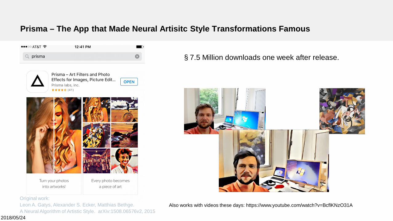
Prisma – The App that Made Neural Artisitc Style Transformations Famous
§ 7.5 Million downloads one week after release.
Also works with videos these days: https://www.youtube.com/watch?v=BcflKNzO31AOriginal work:Leon A. Gatys, Alexander S. Ecker, Matthias Bethge.A Neural Algorithm of Artistic Style. arXiv:1508.06576v2, 2015
2018/05/24
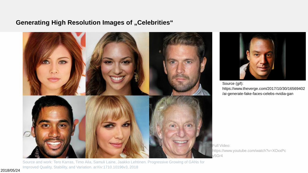
Generating High Resolution Images of „Celebrities“
Source and work: Tero Karras, Timo Aila, Samuli Laine, Jaakko Lehtinen. Progressive Growing of GANs forImproved Quality, Stability, and Variation. arXiv:1710.10196v3, 2018
Full Video:https://www.youtube.com/watch?v=XOxxPcy5Gr4
Source (gif):https://www.theverge.com/2017/10/30/16569402/ai-generate-fake-faces-celebs-nvidia-gan
2018/05/24
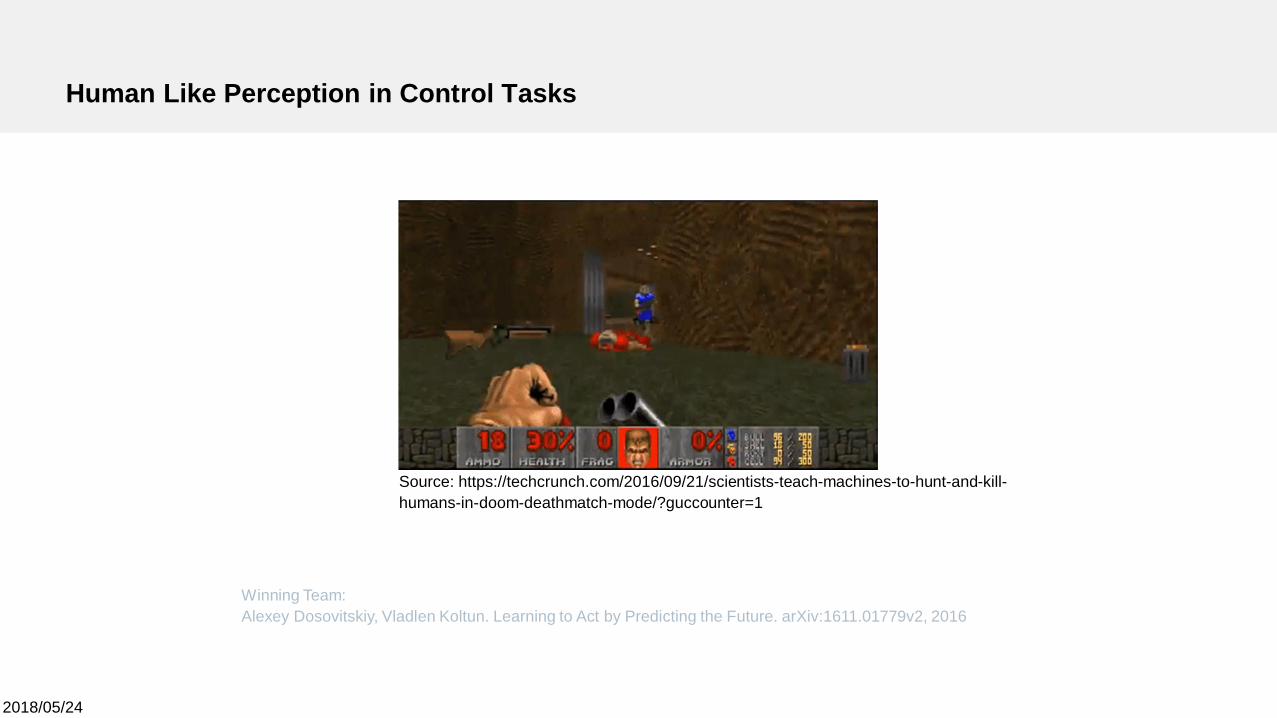
Human Like Perception in Control Tasks
Winning Team:Alexey Dosovitskiy, Vladlen Koltun. Learning to Act by Predicting the Future. arXiv:1611.01779v2, 2016
Source: https://techcrunch.com/2016/09/21/scientists-teach-machines-to-hunt-and-kill-humans-in-doom-deathmatch-mode/?guccounter=1
2018/05/24
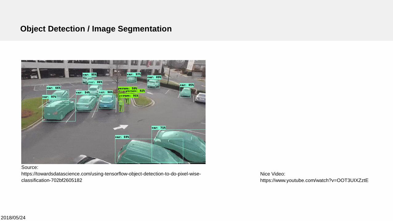
Object Detection / Image Segmentation
Nice Video:https://www.youtube.com/watch?v=OOT3UIXZztE
Source:https://towardsdatascience.com/using-tensorflow-object-detection-to-do-pixel-wise-classification-702bf2605182
2018/05/24
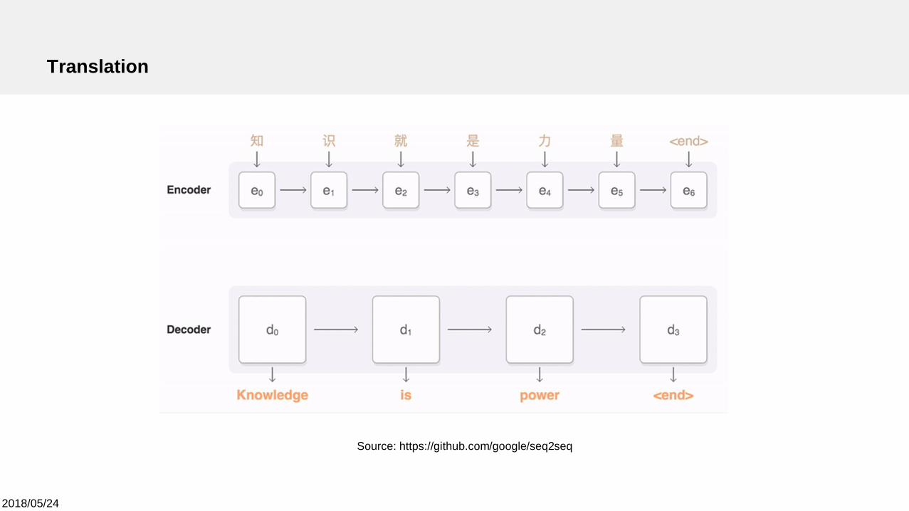
Translation
Source: https://github.com/google/seq2seq

And more…
2018/05/24
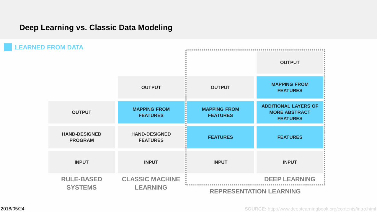
Deep Learning vs. Classic Data Modeling
INPUT
HAND-DESIGNEDPROGRAM
OUTPUT
INPUT
HAND-DESIGNEDFEATURES
MAPPING FROMFEATURES
OUTPUT
INPUT
FEATURES
MAPPING FROMFEATURES
OUTPUT
INPUT
FEATURES
ADDITIONAL LAYERS OFMORE ABSTRACT
FEATURES
MAPPING FROMFEATURES
OUTPUT
RULE-BASEDSYSTEMS
CLASSIC MACHINELEARNING REPRESENTATION LEARNING
DEEP LEARNING
SOURCE: http://www.deeplearningbook.org/contents/intro.html
LEARNED FROM DATA
2018/05/24
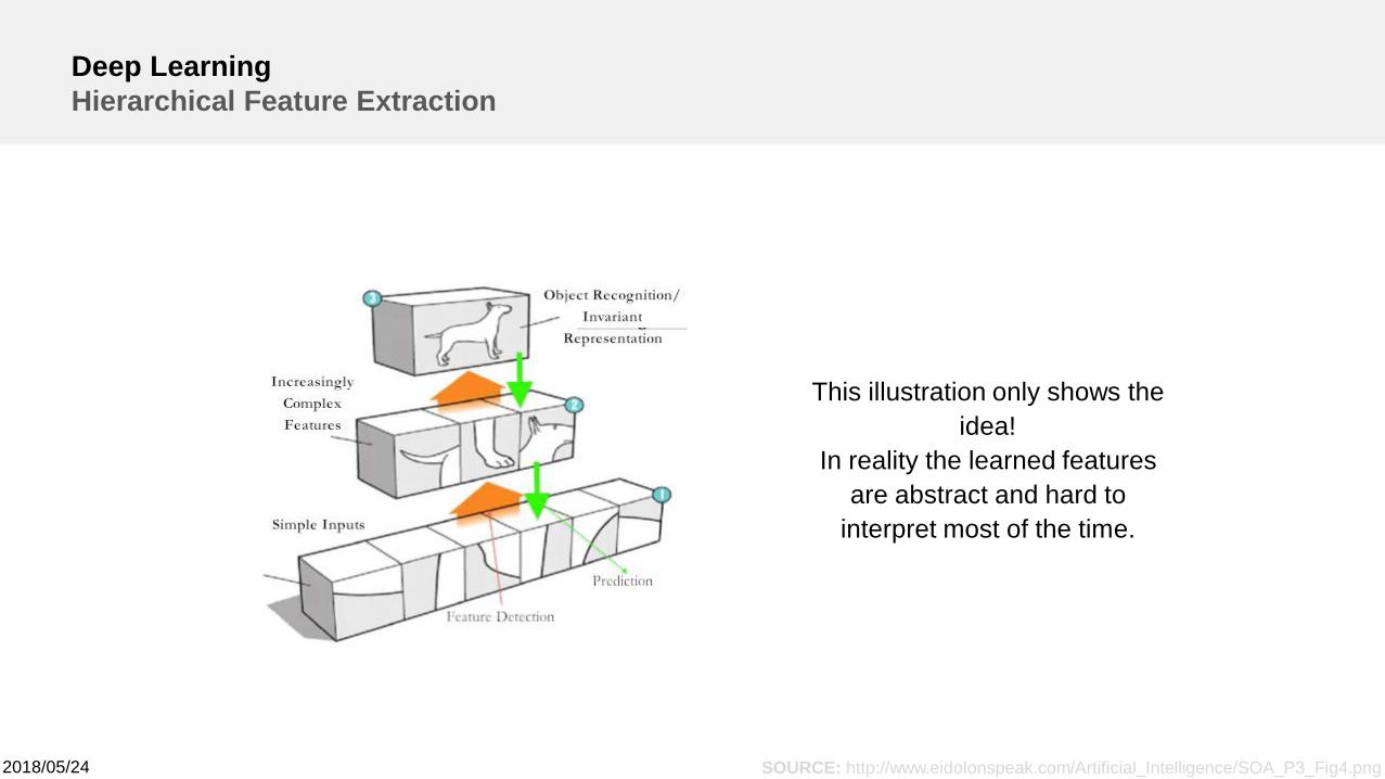
Deep LearningHierarchical Feature Extraction
SOURCE: http://www.eidolonspeak.com/Artificial_Intelligence/SOA_P3_Fig4.png
This illustration only shows theidea!
In reality the learned featuresare abstract and hard to
interpret most of the time.
2018/05/24
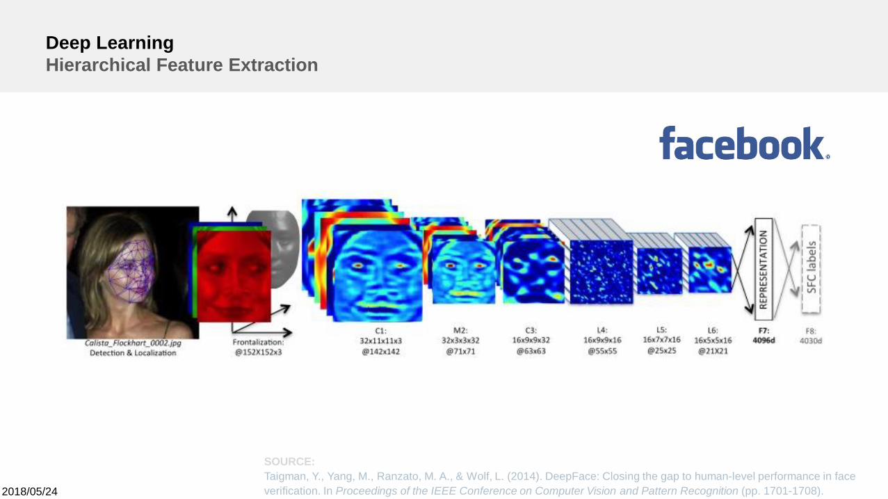
Deep LearningHierarchical Feature Extraction
SOURCE:Taigman, Y., Yang, M., Ranzato, M. A., & Wolf, L. (2014). DeepFace: Closing the gap to human-level performance in faceverification. In Proceedings of the IEEE Conference on Computer Vision and Pattern Recognition (pp. 1701-1708).
(Classic) Neural Networks are an importantbuilding block of Deep Learning but there is more
to it.
NEURAL NETWORKS HAVE BEEN AROUND FOR DECADES!
2018/05/24
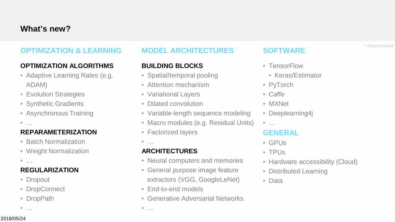
What’s new?
OPTIMIZATION & LEARNING
OPTIMIZATION ALGORITHMS• Adaptive Learning Rates (e.g.
ADAM)• Evolution Strategies• Synthetic Gradients• Asynchronous Training• …REPARAMETERIZATION• Batch Normalization• Weight Normalization• …REGULARIZATION• Dropout• DropConnect• DropPath• …
MODEL ARCHITECTURES
BUILDING BLOCKS• Spatial/temporal pooling• Attention mechanism• Variational Layers• Dilated convolution• Variable-length sequence modeling• Macro modules (e.g. Residual Units)• Factorized layers• …ARCHITECTURES• Neural computers and memories• General purpose image feature
extractors (VGG, GoogleLeNet)• End-to-end models• Generative Adversarial Networks• …
SOFTWARE
• TensorFlow• Keras/Estimator
• PyTorch• Caffe• MXNet• Deeplearning4j• …GENERAL• GPUs• TPUs• Hardware accessibility (Cloud)• Distributed Learning• Data
* deprecated
2018/05/24
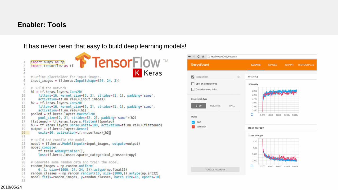
Enabler: Tools
It has never been that easy to build deep learning models!
2018/05/24
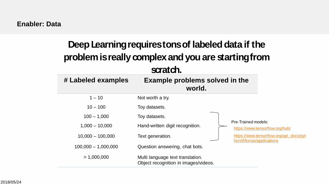
Enabler: Data
Deep Learning requires tons of labeled data if theproblem is really complex and you are starting from
scratch.# Labeled examples Example problems solved in the
world.1 – 10 Not worth a try.
10 – 100 Toy datasets.
100 – 1,000 Toy datasets.
1,000 – 10,000 Hand-written digit recognition.
10,000 – 100,000 Text generation.
100,000 – 1,000,000 Question answering, chat bots.
> 1,000,000 Multi language text translation.Object recognition in images/videos.
https://www.tensorflow.org/hub/
https://www.tensorflow.org/api_docs/python/tf/keras/applications
Pre-Trained models:

2018/05/24
Enabler: Computing Power for Everyone
GPUs
kmmn RWRXWXh ´´ ÎÎ×= ,,
Matrix Products are highly parallelizable Distributed training enables us to train verylarge deep learning models on tons of data
2018/05/24
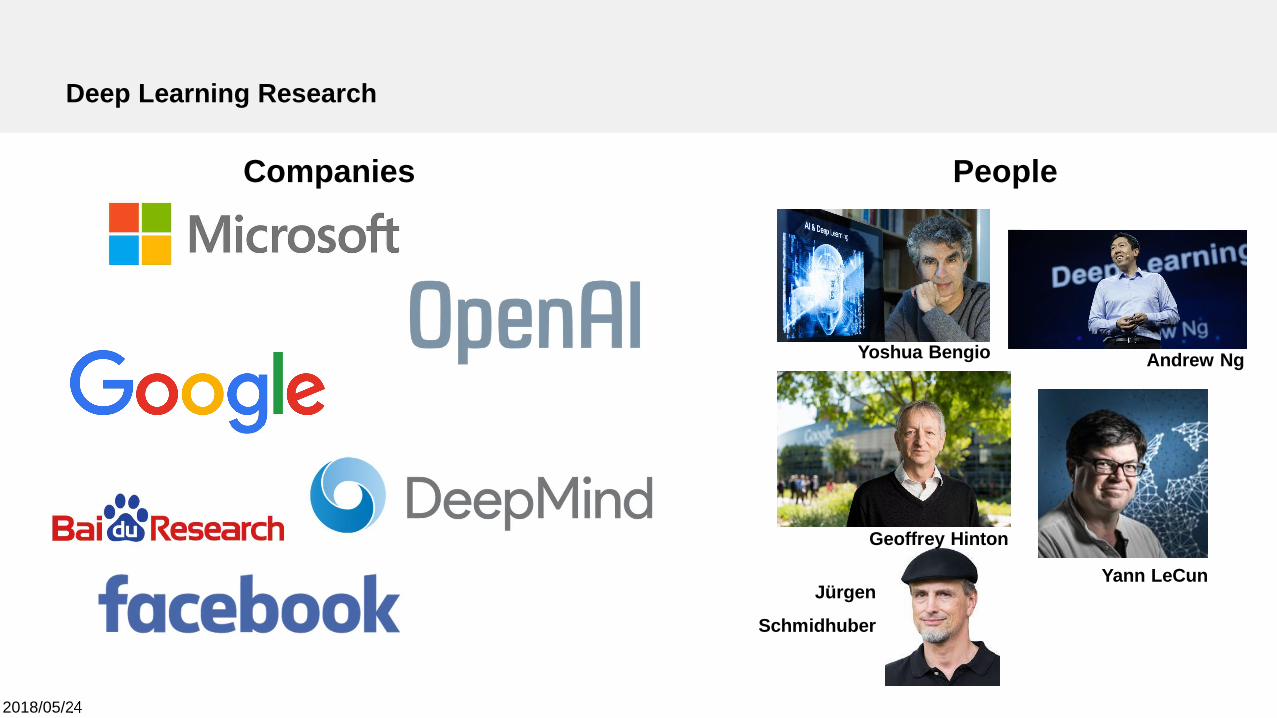
Deep Learning Research
Companies People
Jürgen
Schmidhuber
Geoffrey Hinton
Yann LeCun
Andrew NgYoshua Bengio
Deep LearningImplementation
2018/05/24
Lecture Overview
I. Introduction to Deep Learning
II. Implementation of a Deep Learning Modeli. Overviewii. Model Architecture Design
a. Basic Building Blocksb. Thinking in Macro Structuresc. End-to-End Model Design
iii. Model Traininga. Loss Functionsb. Optimizationc. Regularization
2018/05/24
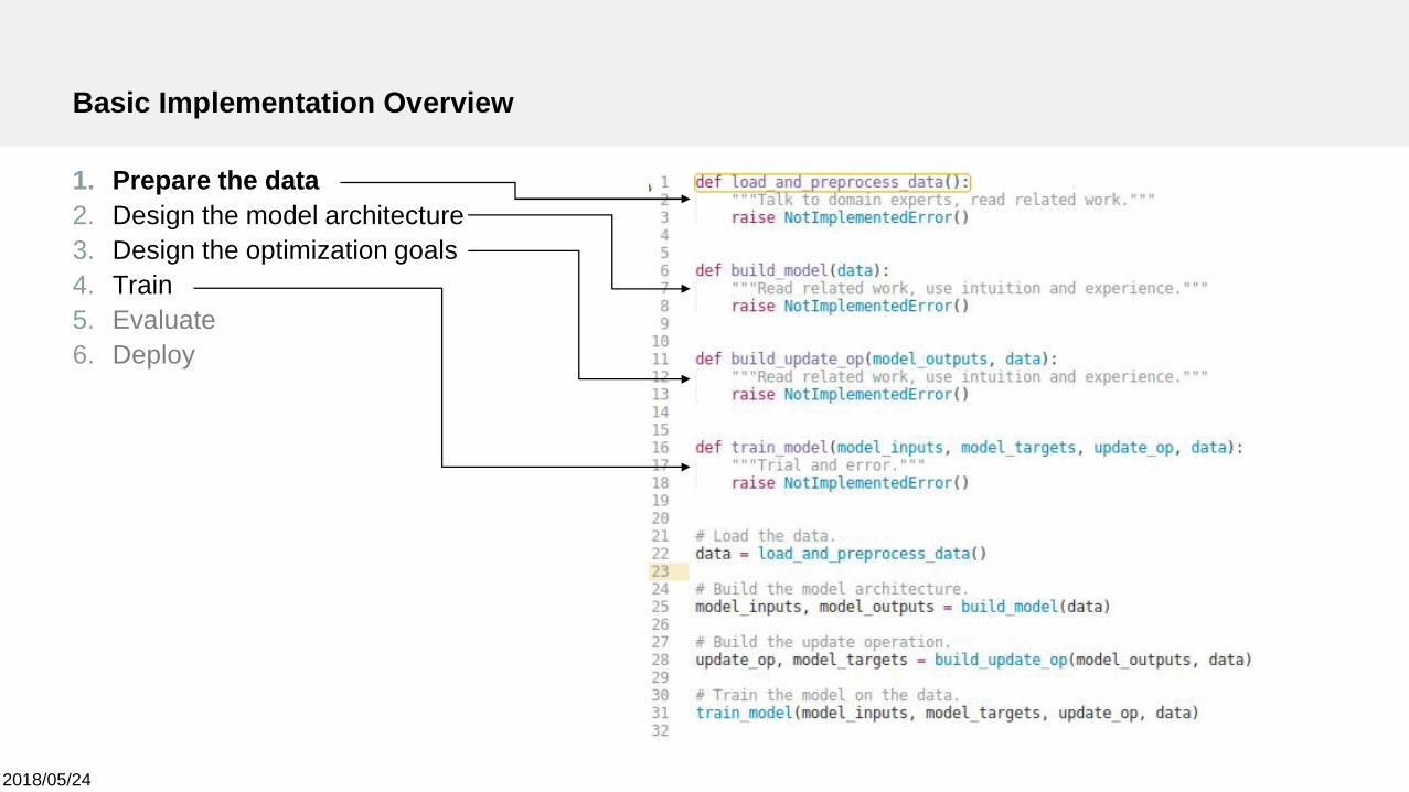
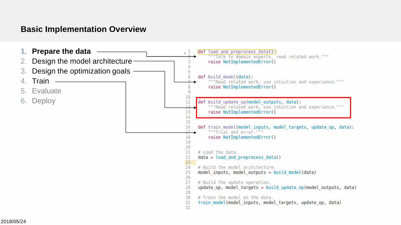
Basic Implementation Overview
1. Prepare the data2. Design the model architecture3. Design the optimization goals4. Train5. Evaluate6. Deploy
2018/05/24
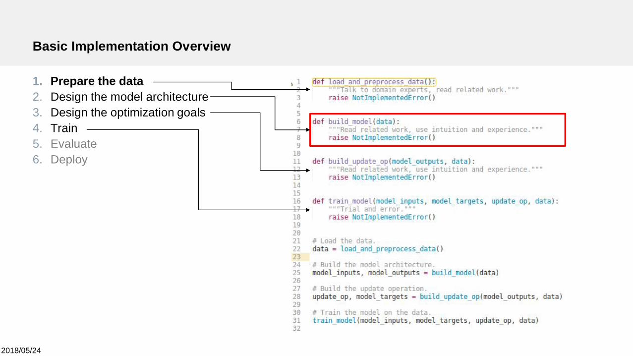
Basic Implementation Overview
1. Prepare the data2. Design the model architecture3. Design the optimization goals4. Train5. Evaluate6. Deploy
2018/05/24
Deep Learning Model Architecture
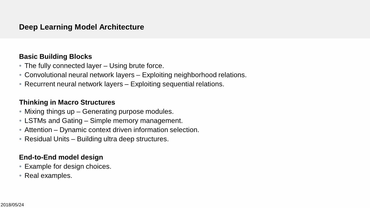
Basic Building Blocks• The fully connected layer – Using brute force.• Convolutional neural network layers – Exploiting neighborhood relations.• Recurrent neural network layers – Exploiting sequential relations.
Thinking in Macro Structures• Mixing things up – Generating purpose modules.• LSTMs and Gating – Simple memory management.• Attention – Dynamic context driven information selection.• Residual Units – Building ultra deep structures.
End-to-End model design• Example for design choices.• Real examples.
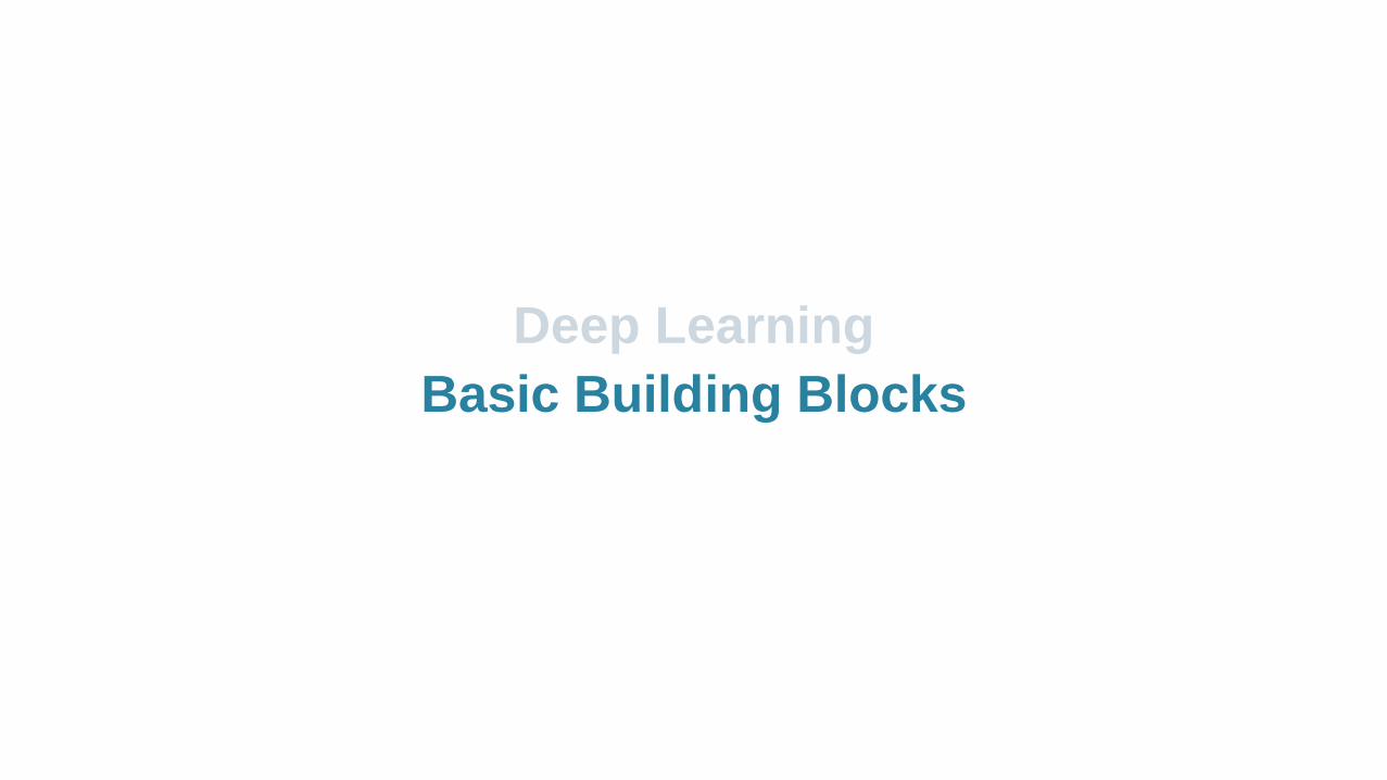
Deep LearningBasic Building Blocks
2018/05/24
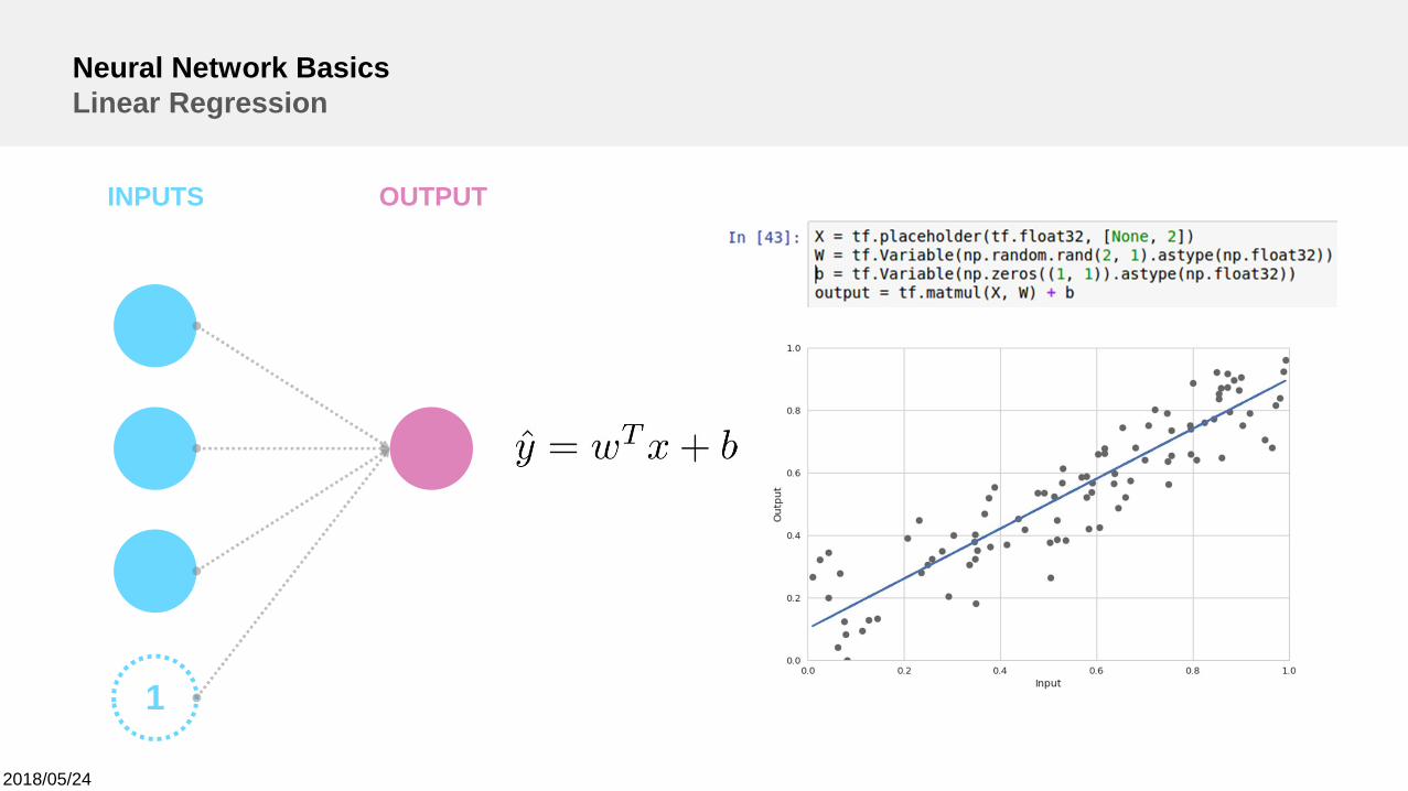
Neural Network BasicsLinear Regression
INPUTS OUTPUT
1
2018/05/24
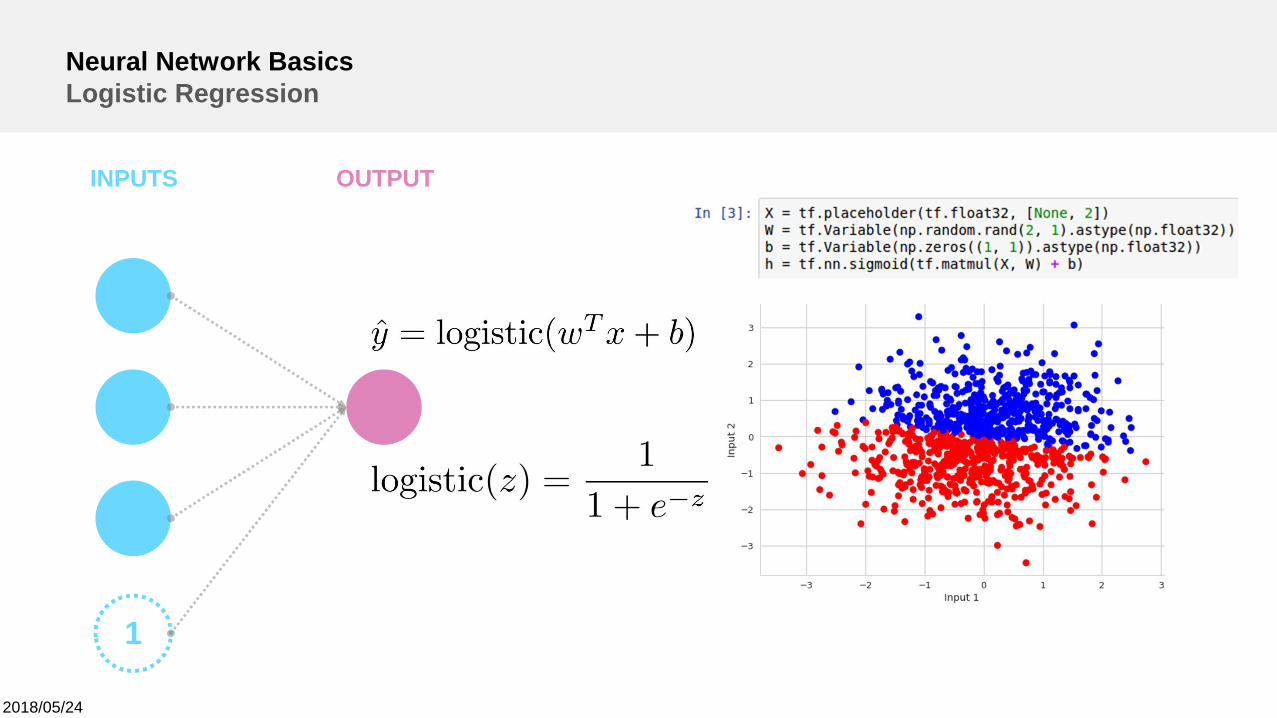
Neural Network BasicsLogistic Regression
INPUTS OUTPUT
1
2018/05/24
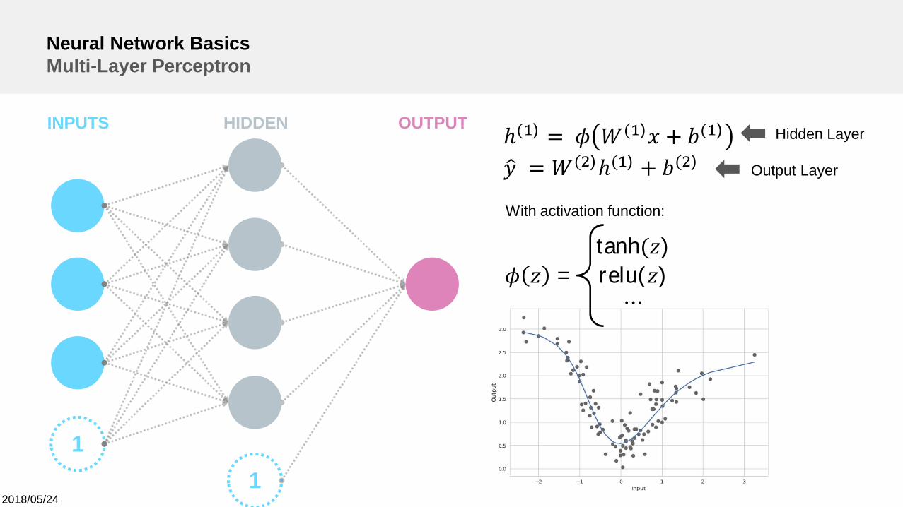
Neural Network BasicsMulti-Layer Perceptron
INPUTS OUTPUTHIDDEN
1
With activation function:
1
Output Layer
Hidden Layerℎ( ) = ( ) + ( )
= ( )ℎ( ) + ( )
tanh( )= relu( )
⋯
2018/05/24
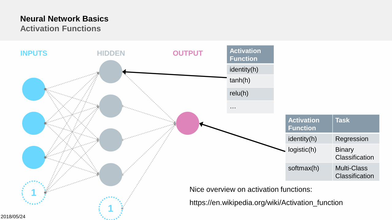
Neural Network BasicsActivation Functions
INPUTS OUTPUTHIDDEN
11
ActivationFunction
Task
identity(h) Regressionlogistic(h) Binary
Classificationsoftmax(h) Multi-Class
Classification
Nice overview on activation functions:
https://en.wikipedia.org/wiki/Activation_function
ActivationFunctionidentity(h)tanh(h)
relu(h)
…
2018/05/24
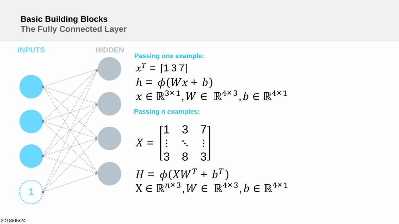
Basic Building BlocksThe Fully Connected Layer
INPUTS HIDDEN
1
Passing one example:
Passing n examples:
= 137
=1 3 7⋮ ⋱ ⋮3 8 3
ℎ = +∈ ℝ × , ∈ ℝ × , ∈ ℝ ×
= +X ∈ ℝ × , ∈ ℝ × , ∈ ℝ ×
2018/05/24
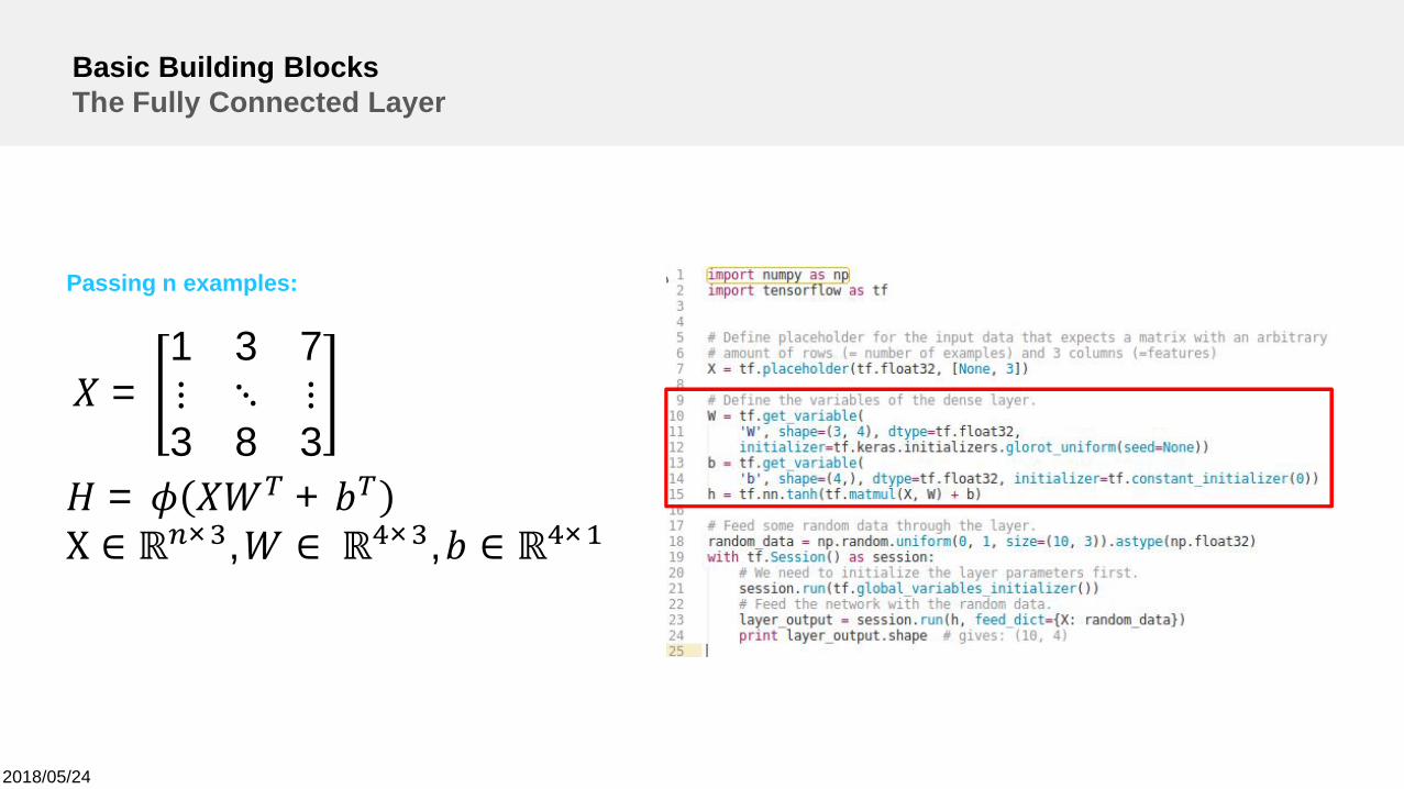
Basic Building BlocksThe Fully Connected Layer
Passing n examples:
=1 3 7⋮ ⋱ ⋮3 8 3
= +X ∈ ℝ × , ∈ ℝ × , ∈ ℝ ×
2018/05/24
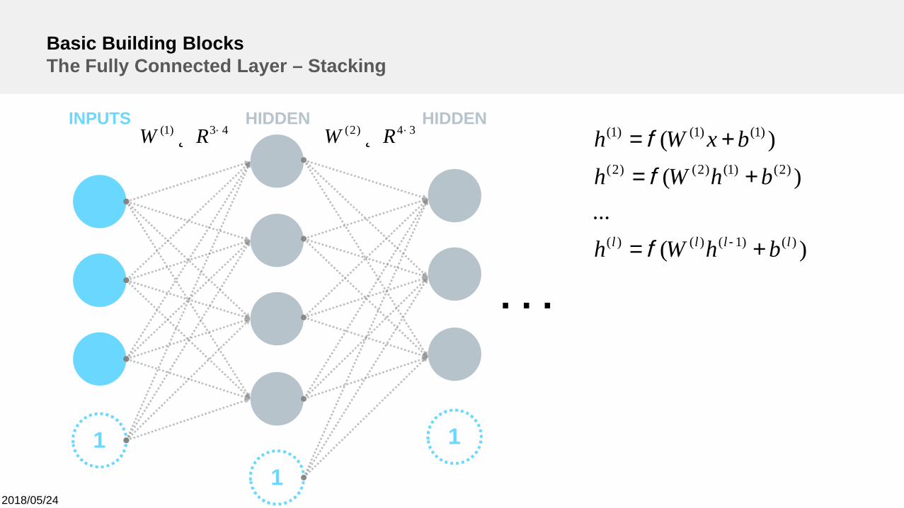
Basic Building BlocksThe Fully Connected Layer – Stacking
INPUTS HIDDEN
11
1
HIDDEN
)(...
)()(
)()1()()(
)2()1()2()2(
)1()1()1(
llll bhWh
bhWhbxWh
+=
+=
+=
-f
f
f
. . .
43)1( ´Î RW 34)2( ´Î RW
2018/05/24
Basic Building BlocksThe Fully Connected Layer – Using Brute Force
INPUTS HIDDEN
1
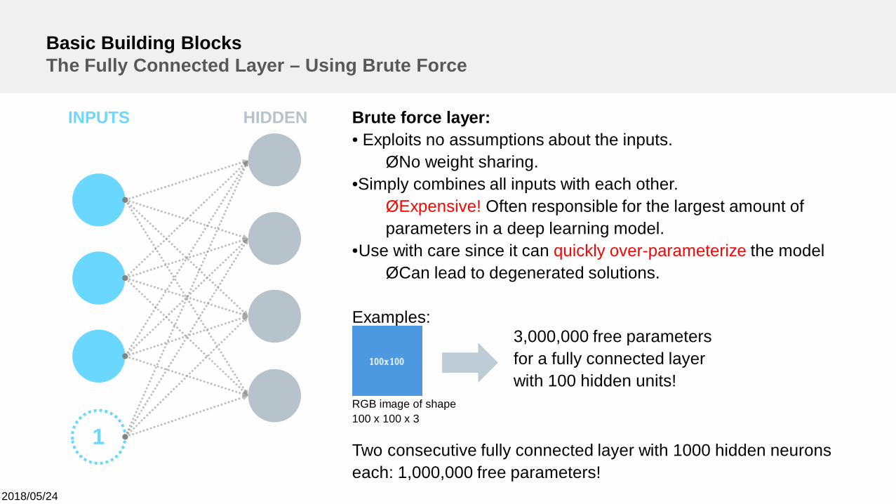
Brute force layer:• Exploits no assumptions about the inputs.ØNo weight sharing.
•Simply combines all inputs with each other.ØExpensive! Often responsible for the largest amount ofparameters in a deep learning model.
•Use with care since it can quickly over-parameterize the modelØCan lead to degenerated solutions.
Examples:
Two consecutive fully connected layer with 1000 hidden neuronseach: 1,000,000 free parameters!
3,000,000 free parametersfor a fully connected layerwith 100 hidden units!
RGB image of shape100 x 100 x 3
2018/05/24
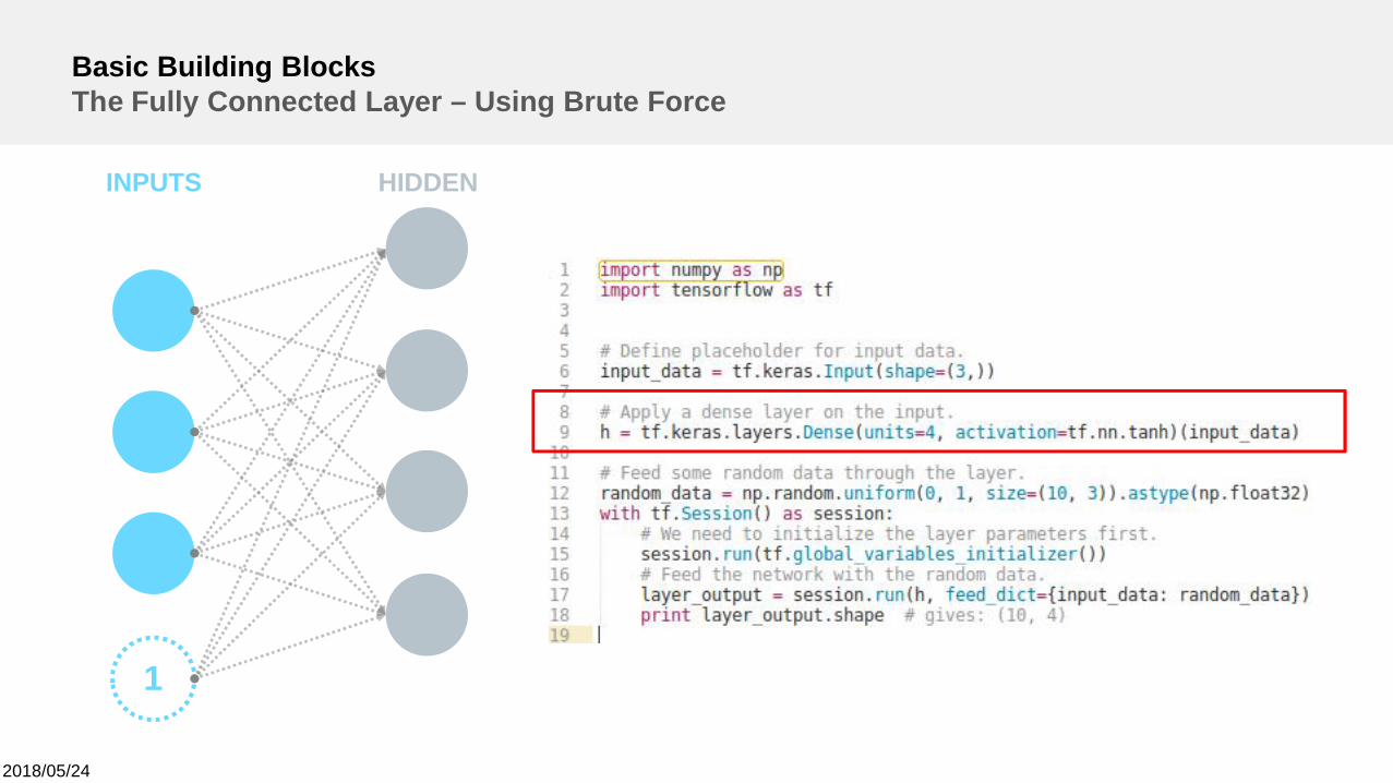
Basic Building BlocksThe Fully Connected Layer – Using Brute Force
INPUTS HIDDEN
1
2018/05/24
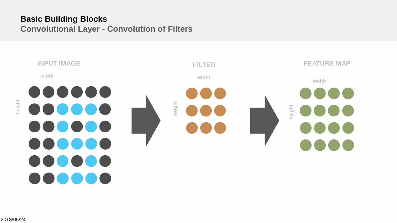
Basic Building BlocksConvolutional Layer - Convolution of Filters
width
heig
ht
INPUT IMAGE
width
heig
ht
FILTER FEATURE MAP
width
heig
ht
2018/05/24
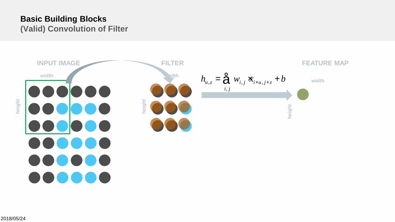
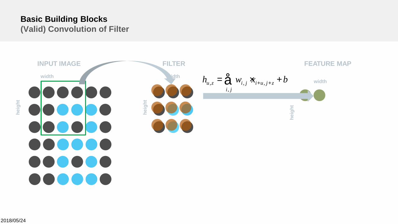
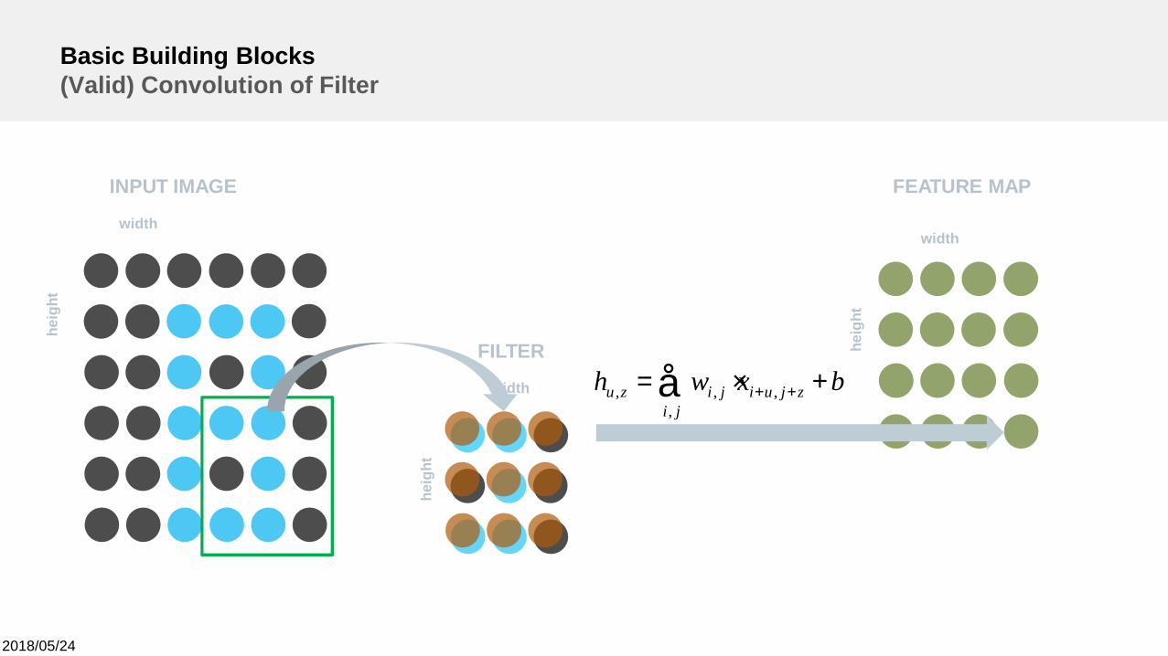
Basic Building Blocks(Valid) Convolution of Filter
width
heig
ht
INPUT IMAGE
width
heig
ht
FILTER FEATURE MAP
width
heig
ht
bxwh zjuiji
jizu +×= ++å ,,
,,
2018/05/24
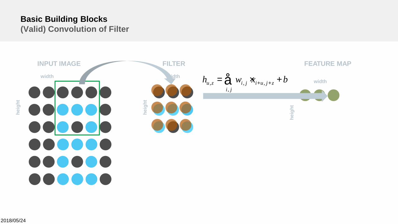
Basic Building Blocks(Valid) Convolution of Filter
width
heig
ht
INPUT IMAGE
width
heig
ht
FILTER FEATURE MAP
width
heig
ht
bxwh zjuiji
jizu +×= ++å ,,
,,
2018/05/24
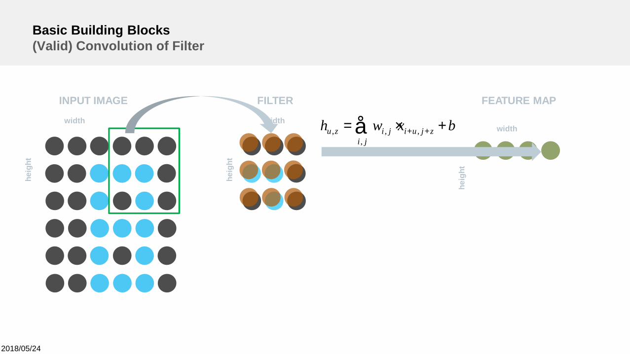
Basic Building Blocks(Valid) Convolution of Filter
width
heig
ht
INPUT IMAGE
width
heig
ht
FILTER FEATURE MAP
width
heig
ht
bxwh zjuiji
jizu +×= ++å ,,
,,
2018/05/24
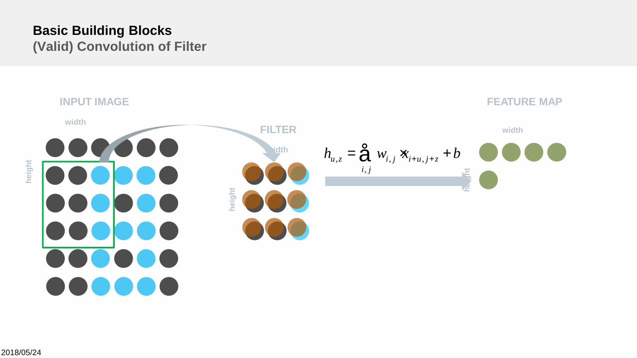
Basic Building Blocks(Valid) Convolution of Filter
width
heig
ht
INPUT IMAGE
width
heig
ht
FILTER FEATURE MAP
width
heig
ht
bxwh zjuiji
jizu +×= ++å ,,
,,
2018/05/24
Basic Building Blocks(Valid) Convolution of Filter
width
heig
ht
INPUT IMAGE
width
heig
ht
FILTER
FEATURE MAP
width
heig
ht
bxwh zjuiji
jizu +×= ++å ,,
,,
2018/05/24
Basic Building Blocks(Valid) Convolution of Filter
width
heig
ht
INPUT IMAGE
width
heig
ht
FILTER
FEATURE MAP
width
heig
ht
bxwh zjuiji
jizu +×= ++å ,,
,,
2018/05/24
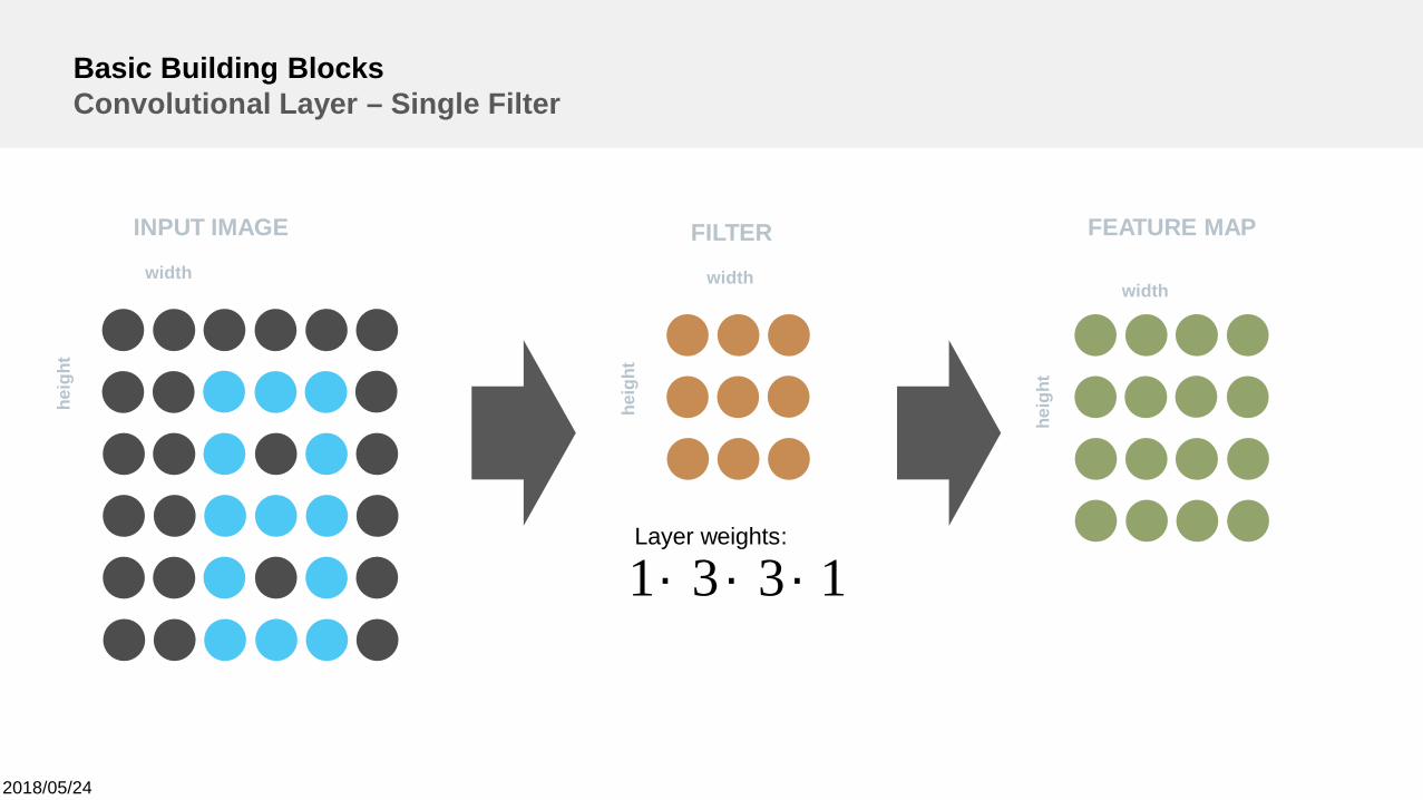
Basic Building BlocksConvolutional Layer – Single Filter
width
heig
ht
INPUT IMAGE
width
heig
ht
FILTER FEATURE MAP
width
heig
ht
1331 ´´´Layer weights:
2018/05/24
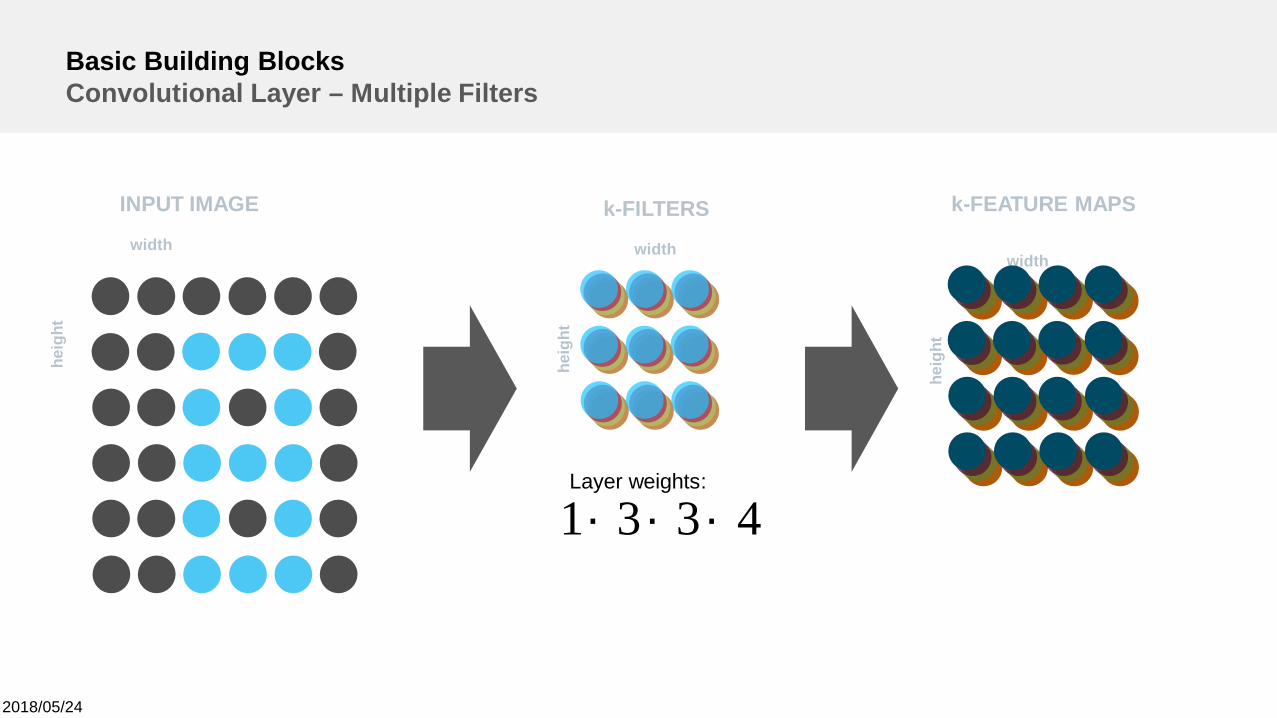
Basic Building BlocksConvolutional Layer – Multiple Filters
width
heig
ht
INPUT IMAGE
width
heig
ht
k-FILTERS k-FEATURE MAPS
width
heig
ht
4331 ´´´Layer weights:
2018/05/24
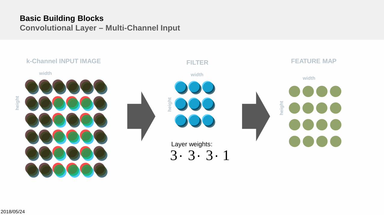
Basic Building BlocksConvolutional Layer – Multi-Channel Input
width
heig
ht
k-Channel INPUT IMAGE
width
heig
ht
FILTER FEATURE MAP
width
heig
ht
1333 ´´´Layer weights:
2018/05/24
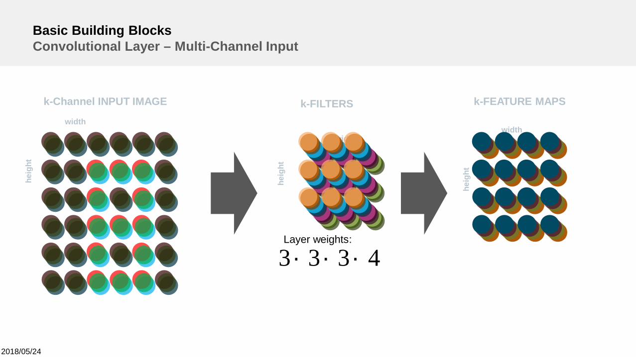
Basic Building BlocksConvolutional Layer – Multi-Channel Input
width
heig
ht
k-Channel INPUT IMAGE
width
heig
ht
k-FILTERS k-FEATURE MAPS
width
heig
ht
4333 ´´´Layer weights:
2018/05/24
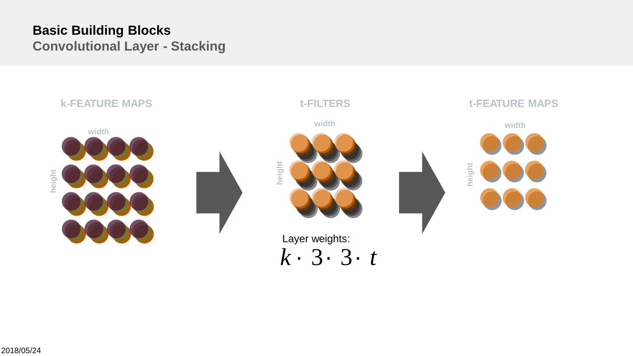
Basic Building BlocksConvolutional Layer - Stacking
width
heig
ht
t-FILTERSk-FEATURE MAPS
width
heig
ht
width
heig
ht
t-FEATURE MAPS
tk ´´´ 33Layer weights:
2018/05/24
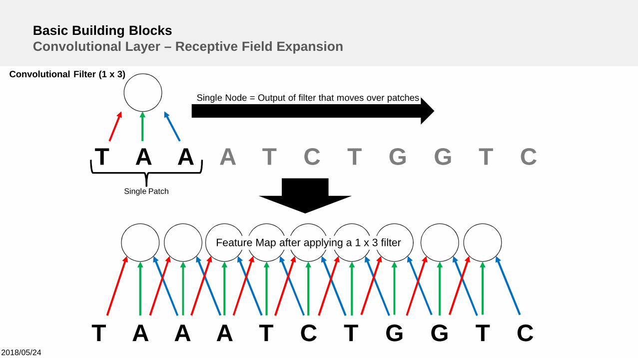
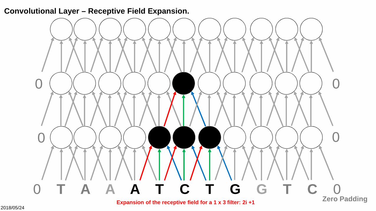
Basic Building BlocksConvolutional Layer – Receptive Field Expansion
T A A A T C T G G T C
Convolutional Filter (1 x 3)
Single Node = Output of filter that moves over patches
Single Patch
Feature Map after applying a 1 x 3 filter
0 T A A A T C T G G T C 0
2018/05/24
0 T A A A T C T G G T C 0
0 0
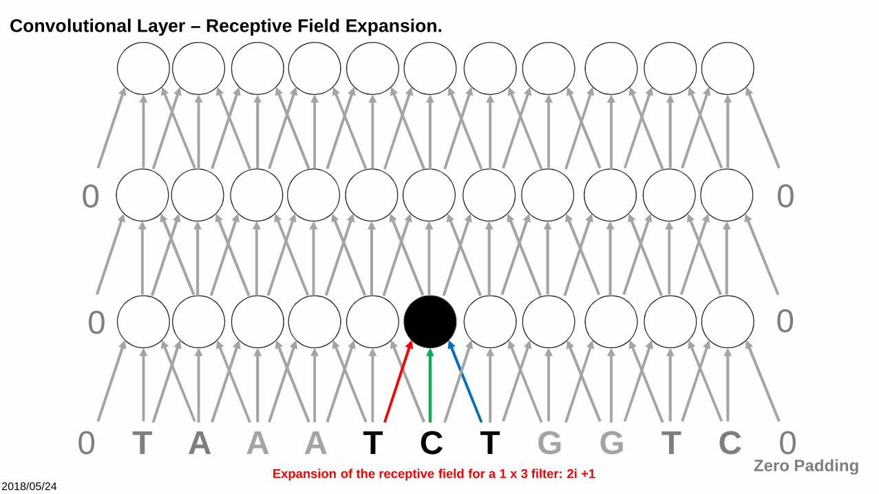
Zero Padding
Convolutional Layer – Receptive Field Expansion.
00
Expansion of the receptive field for a 1 x 3 filter: 2i +1
2018/05/24
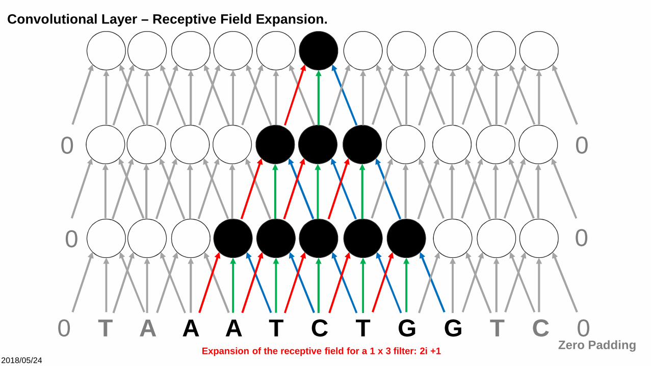
0 T A A A T C T G G T C 0
0 0
Zero Padding
Convolutional Layer – Receptive Field Expansion.
00
Expansion of the receptive field for a 1 x 3 filter: 2i +1
2018/05/24
0 T A A A T C T G G T C 0
0 0
Zero Padding
Convolutional Layer – Receptive Field Expansion.
00
Expansion of the receptive field for a 1 x 3 filter: 2i +1
2018/05/24
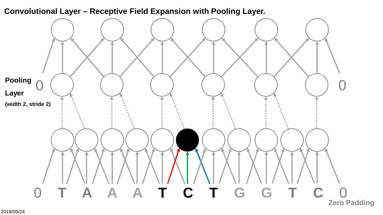
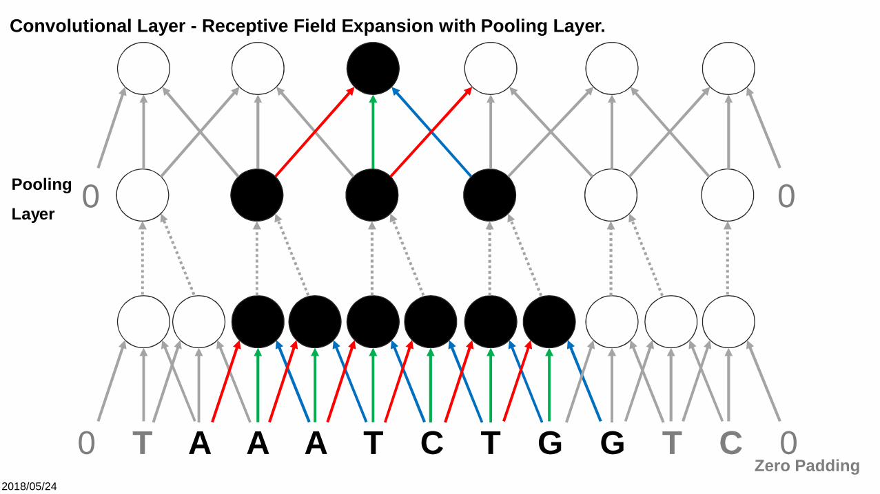
0 T A A A T C T G G T C 0Zero Padding
Convolutional Layer – Receptive Field Expansion with Pooling Layer.
00Pooling
Layer(width 2, stride 2)
2018/05/24
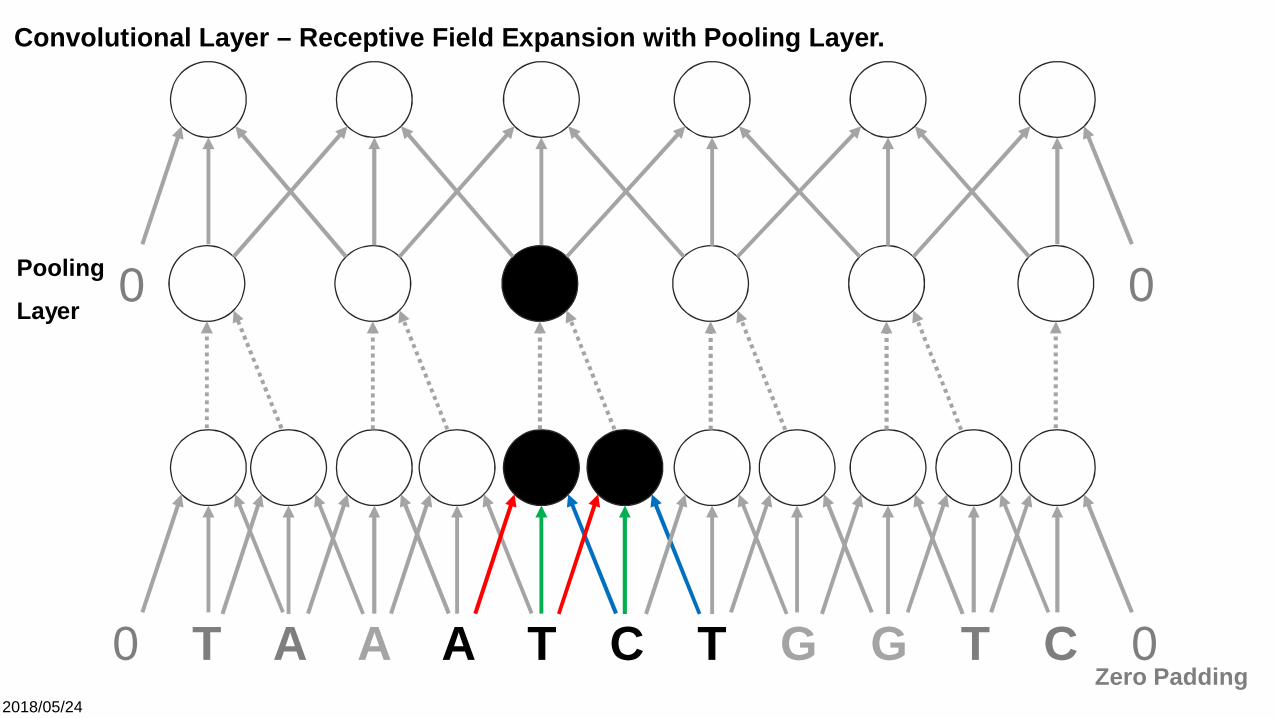
0 T A A A T C T G G T C 0Zero Padding
Convolutional Layer – Receptive Field Expansion with Pooling Layer.
00Pooling
Layer
2018/05/24
0 T A A A T C T G G T C 0Zero Padding
Convolutional Layer - Receptive Field Expansion with Pooling Layer.
00Pooling
Layer
2018/05/24
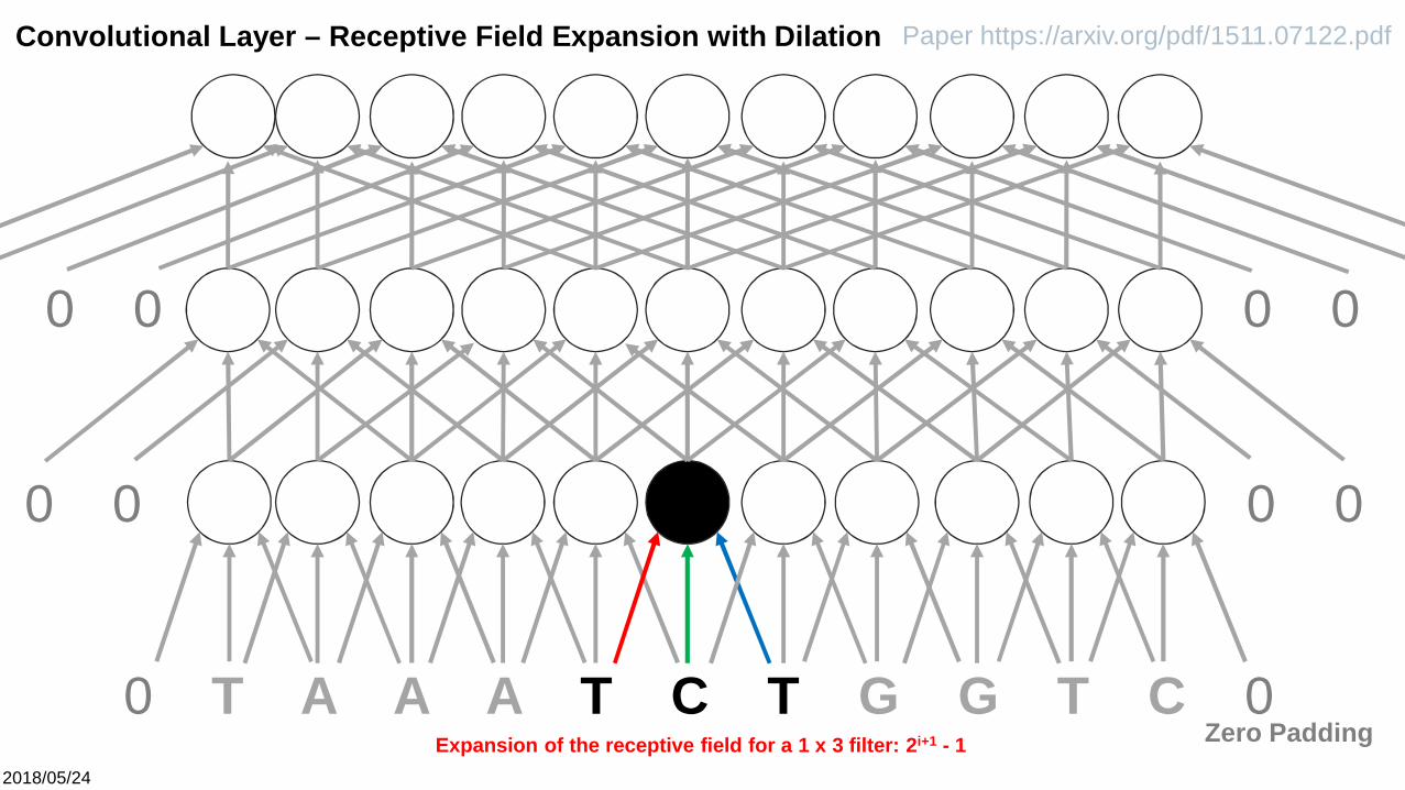
0 T A A A T C T G G T C 0
0 0 0 0
0 00 0
Zero Padding
Convolutional Layer – Receptive Field Expansion with Dilation
Expansion of the receptive field for a 1 x 3 filter: 2i+1 - 1
Paper https://arxiv.org/pdf/1511.07122.pdf
2018/05/24
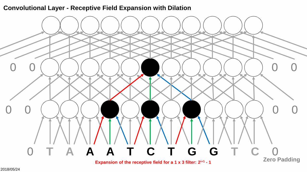
0 T A A A T C T G G T C 0
0 0 0 0
0 00 0
Zero Padding
Convolutional Layer - Receptive Field Expansion with Dilation
Expansion of the receptive field for a 1 x 3 filter: 2i+1 - 1
2018/05/24
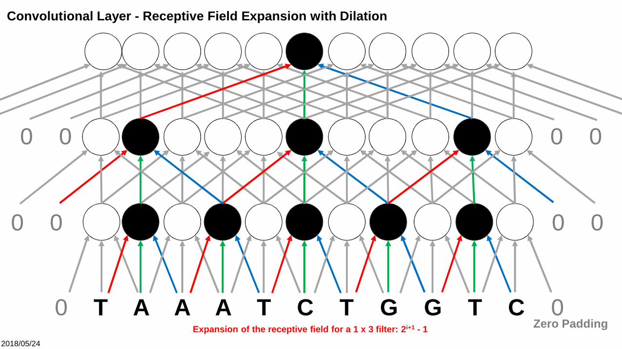
0 T A A A T C T G G T C 0
0 0 0 0
0 00 0
Zero Padding
Convolutional Layer - Receptive Field Expansion with Dilation
Expansion of the receptive field for a 1 x 3 filter: 2i+1 - 1
2018/05/24
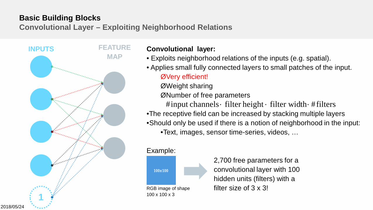
Basic Building BlocksConvolutional Layer – Exploiting Neighborhood Relations
INPUTS FEATUREMAP
Convolutional layer:• Exploits neighborhood relations of the inputs (e.g. spatial).• Applies small fully connected layers to small patches of the input.ØVery efficient!ØWeight sharingØNumber of free parameters
•The receptive field can be increased by stacking multiple layers•Should only be used if there is a notion of neighborhood in the input:
•Text, images, sensor time-series, videos, …
Example:2,700 free parameters for aconvolutional layer with 100hidden units (filters) with afilter size of 3 x 3!RGB image of shape
100 x 100 x 3
filters#thfilter widheightfilterchannelsinput# ´´´
1
2018/05/24
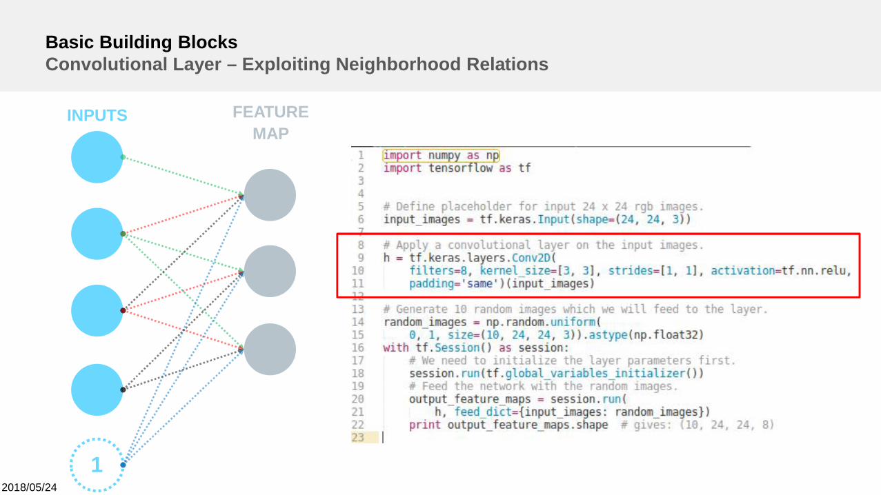
Basic Building BlocksConvolutional Layer – Exploiting Neighborhood Relations
INPUTS FEATUREMAP
1
2018/05/24
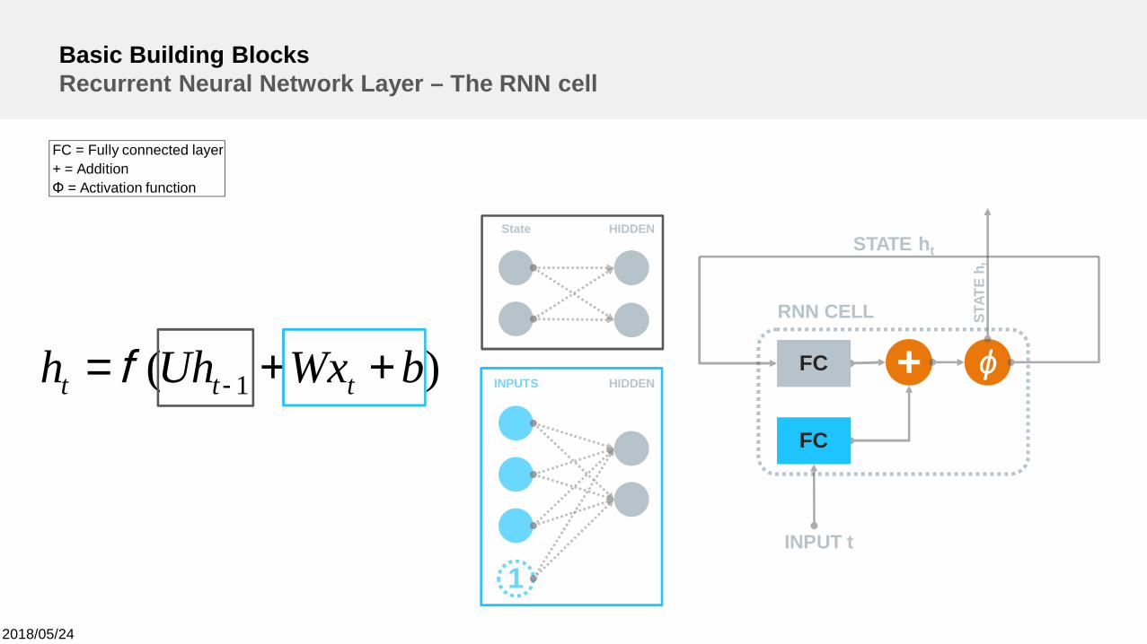
Basic Building BlocksRecurrent Neural Network Layer – The RNN cell
+RNN CELL
INPUT t
ϕFC
FC
STAT
Eh t
STATE ht
FC = Fully connected layer+ = AdditionΦ = Activation function
INPUTS HIDDEN
1
State HIDDEN
)( 1 bWxUhh ttt ++= -f
2018/05/24
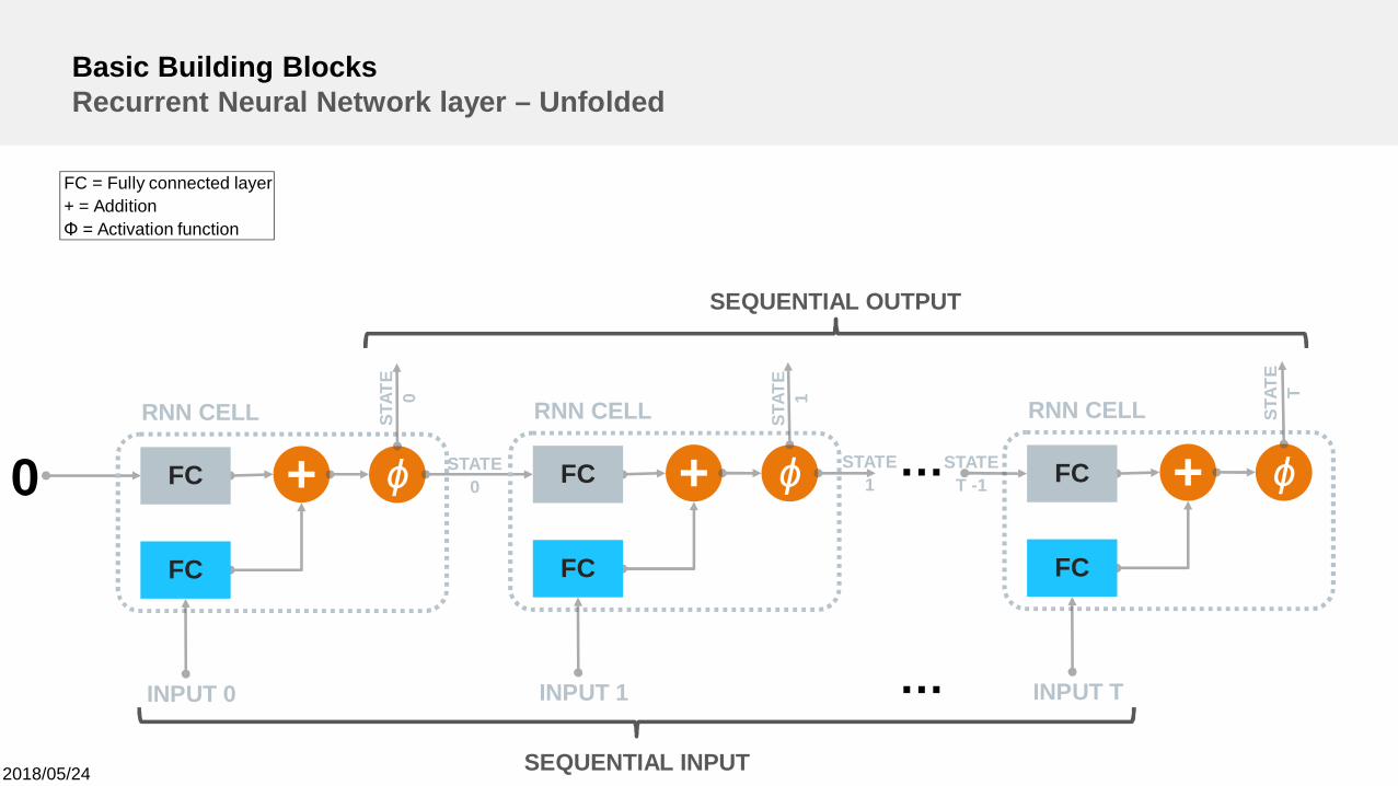
Basic Building BlocksRecurrent Neural Network layer – Unfolded
+0RNN CELL
INPUT 0
ϕFC
FC
+RNN CELL
INPUT 1
ϕFC
FC
STAT
E0
STATE0 +
RNN CELL
INPUT T
ϕFC
FC
…
…
STATE1
STATET -1
FC = Fully connected layer+ = AdditionΦ = Activation function
STAT
E1
STAT
ET
SEQUENTIAL INPUT
SEQUENTIAL OUTPUT
2018/05/24
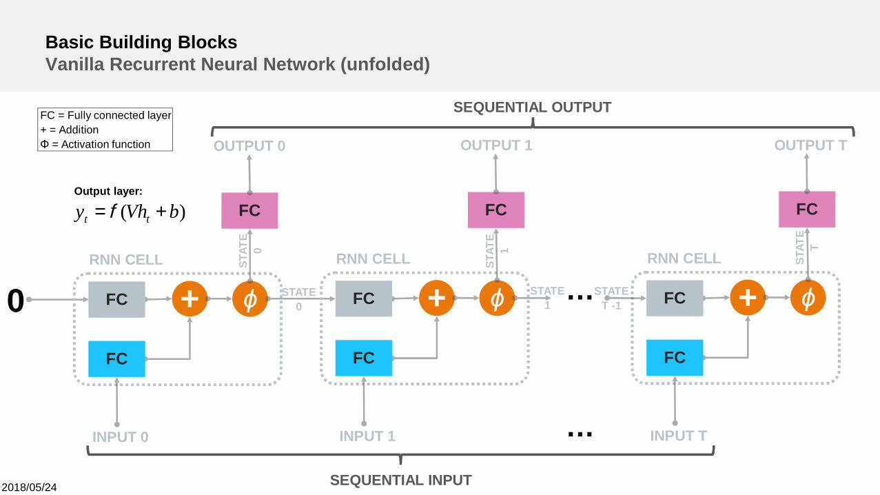
Basic Building BlocksVanilla Recurrent Neural Network (unfolded)
+0RNN CELL
INPUT 0
ϕFC
FC
FC
OUTPUT 0
+RNN CELL
INPUT 1
ϕFC
FC
FC
OUTPUT 1
STAT
E0
STATE0 +
RNN CELL
INPUT T
ϕFC
FC
FC
OUTPUT T
…
…
STATE1
STATET -1
SEQUENTIAL INPUT
SEQUENTIAL OUTPUTFC = Fully connected layer+ = AdditionΦ = Activation function
STAT
E1
STAT
ET
)( bVhy tt += fOutput layer:
2018/05/24
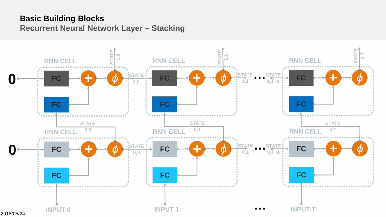
Basic Building BlocksRecurrent Neural Network Layer – Stacking
+0RNN CELL
INPUT 0
ϕFC
FC
+RNN CELL
INPUT 1
ϕFC
FC
STATE0,0
STATE0,0 +
RNN CELL
INPUT T
ϕFC
FC
…
…
STATE0,1
STATE0,T -1
STATE0,1
STATE0,T
+0RNN CELL
ϕFC
FC
+RNN CELL
ϕFC
FCST
ATE
1,0
STATE1,0 +
RNN CELL
ϕFC
FC
…STATE1,1
STATE1,T -1
STAT
E1,
1
STAT
E1,
T
2018/05/24
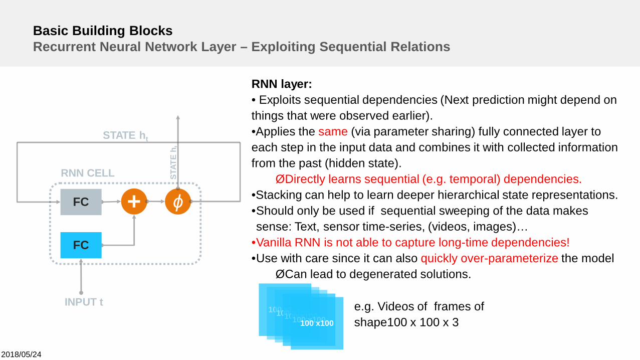
Basic Building BlocksRecurrent Neural Network Layer – Exploiting Sequential Relations
RNN layer:• Exploits sequential dependencies (Next prediction might depend onthings that were observed earlier).•Applies the same (via parameter sharing) fully connected layer toeach step in the input data and combines it with collected informationfrom the past (hidden state).ØDirectly learns sequential (e.g. temporal) dependencies.
•Stacking can help to learn deeper hierarchical state representations.•Should only be used if sequential sweeping of the data makessense: Text, sensor time-series, (videos, images)…
•Vanilla RNN is not able to capture long-time dependencies!•Use with care since it can also quickly over-parameterize the model
ØCan lead to degenerated solutions.
100 x100100 x100100 x100100 x100100 x100
e.g. Videos of frames ofshape100 x 100 x 3
+RNN CELL
INPUT t
ϕFC
FC
STAT
Eh t
STATE ht
2018/05/24
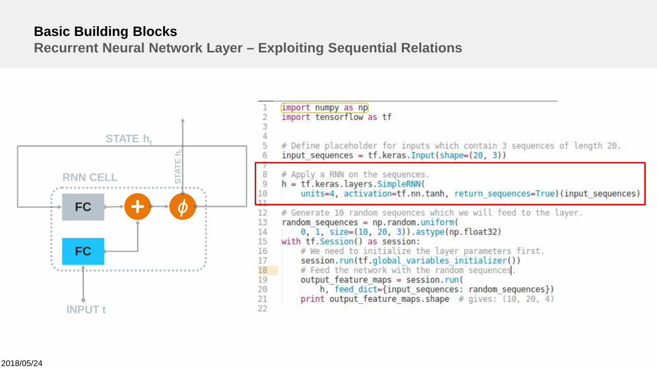
Basic Building BlocksRecurrent Neural Network Layer – Exploiting Sequential Relations
+RNN CELL
INPUT t
ϕFC
FC
STAT
Eh t
STATE ht
Deep LearningThinking in Macro Structures
2018/05/24
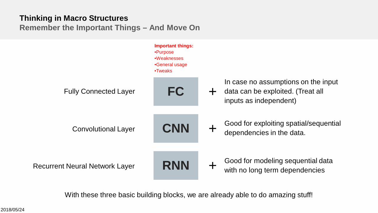
Thinking in Macro StructuresRemember the Important Things – And Move On
In case no assumptions on the inputdata can be exploited. (Treat allinputs as independent)
FC +
Good for exploiting spatial/sequentialdependencies in the data.CNN +
Good for modeling sequential datawith no long term dependenciesRNN +
Fully Connected Layer
Convolutional Layer
Recurrent Neural Network Layer
With these three basic building blocks, we are already able to do amazing stuff!
Important things:•Purpose•Weaknesses•General usage•Tweaks
2018/05/24
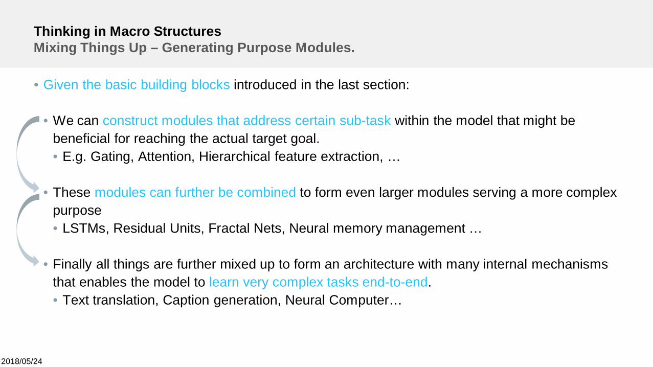
Thinking in Macro StructuresMixing Things Up – Generating Purpose Modules.
• Given the basic building blocks introduced in the last section:
• We can construct modules that address certain sub-task within the model that might bebeneficial for reaching the actual target goal.• E.g. Gating, Attention, Hierarchical feature extraction, …
• These modules can further be combined to form even larger modules serving a more complexpurpose• LSTMs, Residual Units, Fractal Nets, Neural memory management …
• Finally all things are further mixed up to form an architecture with many internal mechanismsthat enables the model to learn very complex tasks end-to-end.• Text translation, Caption generation, Neural Computer…
2018/05/24
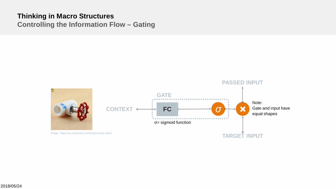
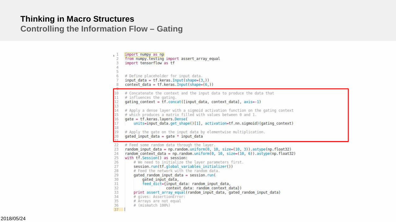
Thinking in Macro StructuresControlling the Information Flow – Gating
Image: https://au.pinterest.com/explore/tap-valve/ TARGET INPUT
σFCCONTEXT
PASSED INPUT
GATE
σ= sigmoid function
Note:Gate and input haveequal shapes
2018/05/24
Thinking in Macro StructuresControlling the Information Flow – Gating
Note:Gate and input haveequal shapes
Add implementation
2018/05/24
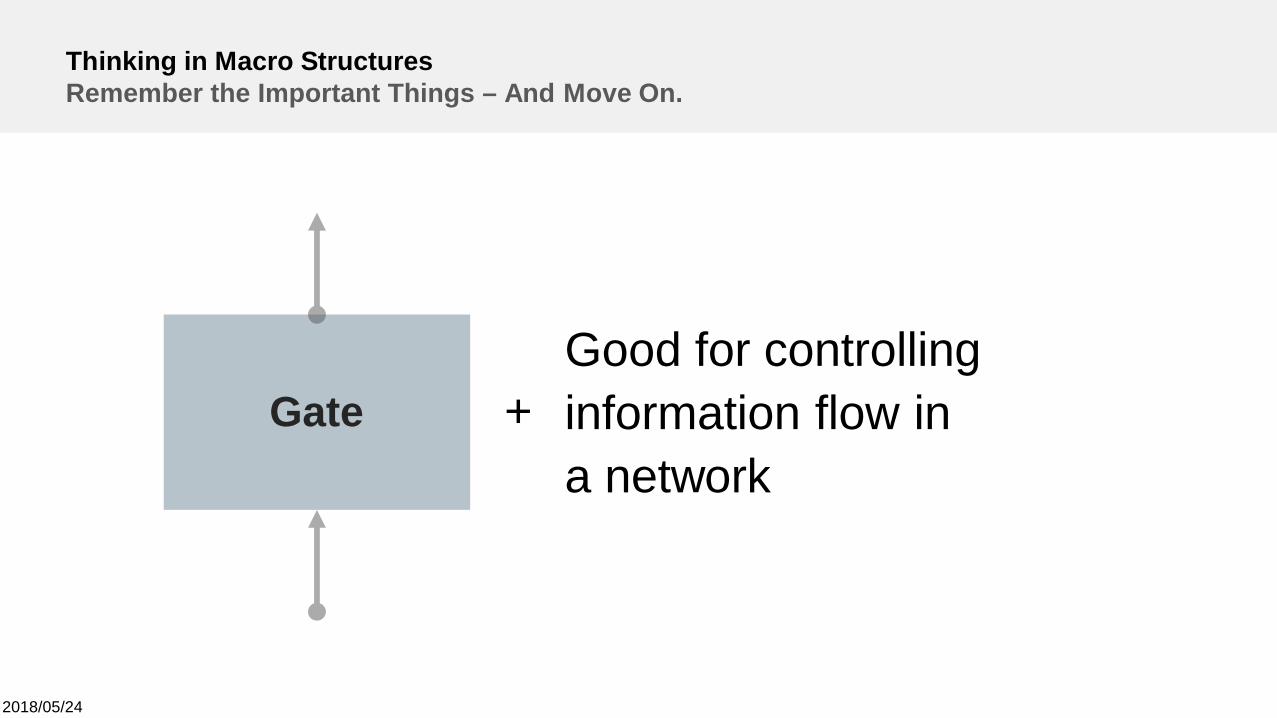
Thinking in Macro StructuresRemember the Important Things – And Move On.
GateGood for controllinginformation flow ina network
+
2018/05/24
ttt
ototot
ctctctttt
itittt
ftfttt
cohbhUxWo
bhUxWicfcbhUxWi
bhUxWf
×=++=
++×+×=++=
++=
-
--
-
-
)()(
)(
)(
1
11
1
1
sf
s
s
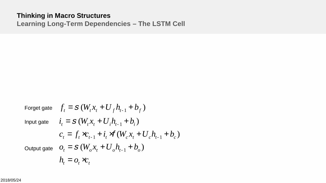
Thinking in Macro StructuresLearning Long-Term Dependencies – The LSTM Cell
Forget gate
Input gate
Output gate
2018/05/24
CELL STATE ct
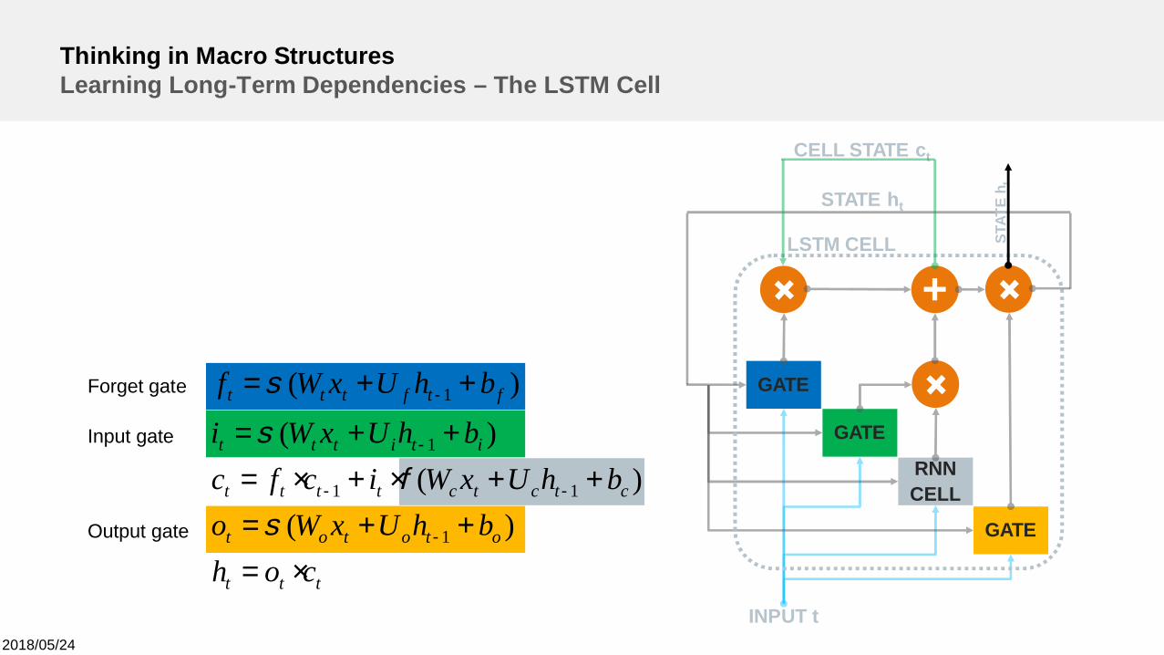
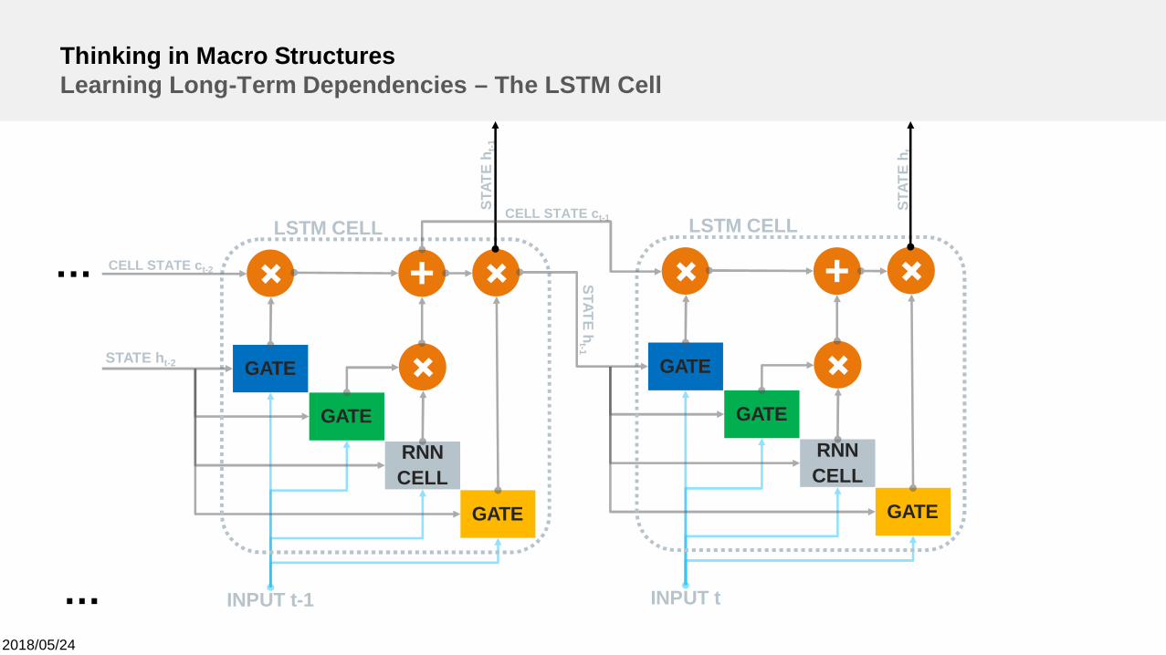
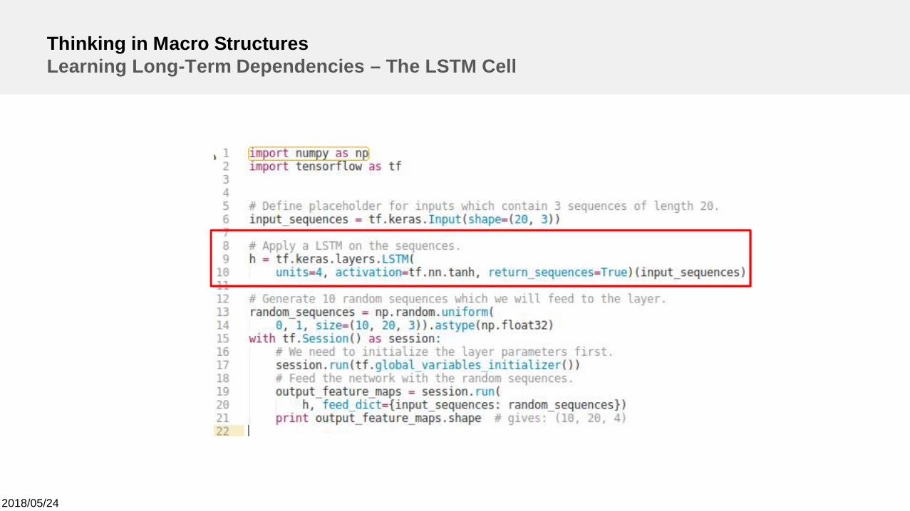
Thinking in Macro StructuresLearning Long-Term Dependencies – The LSTM Cell
LSTM CELL
GATE
INPUT t
GATE
RNNCELL
+
GATE
STAT
Eh tSTATE ht
ttt
ototot
ctctctttt
itittt
ftfttt
cohbhUxWo
bhUxWicfcbhUxWi
bhUxWf
×=++=
++×+×=++=
++=
-
--
-
-
)()(
)(
)(
1
11
1
1
sf
s
sForget gate
Input gate
Output gate
2018/05/24
Thinking in Macro StructuresLearning Long-Term Dependencies – The LSTM Cell
STATEh
t-1
…
…
LSTM CELL
GATE
INPUT t-1
GATE
RNNCELL
+
GATEST
ATE
h t-1
CELL STATE ct-1 LSTM CELL
GATE
INPUT t
GATE
RNNCELL
+
GATE
STAT
Eh t
CELL STATE ct-2
STATE ht-2
2018/05/24
Thinking in Macro StructuresLearning Long-Term Dependencies – The LSTM Cell
2018/05/24
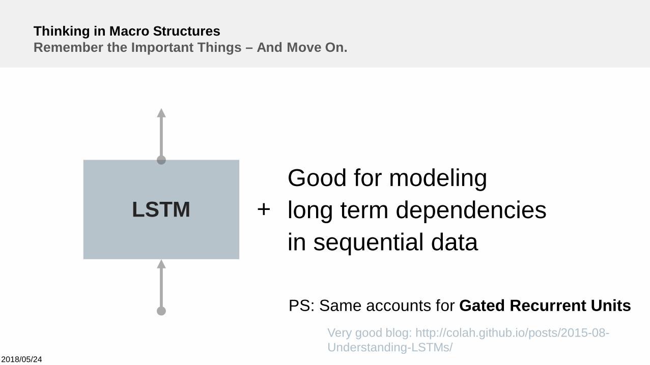
Thinking in Macro StructuresRemember the Important Things – And Move On.
LSTMGood for modelinglong term dependenciesin sequential data
+
PS: Same accounts for Gated Recurrent UnitsVery good blog: http://colah.github.io/posts/2015-08-Understanding-LSTMs/
2018/05/24
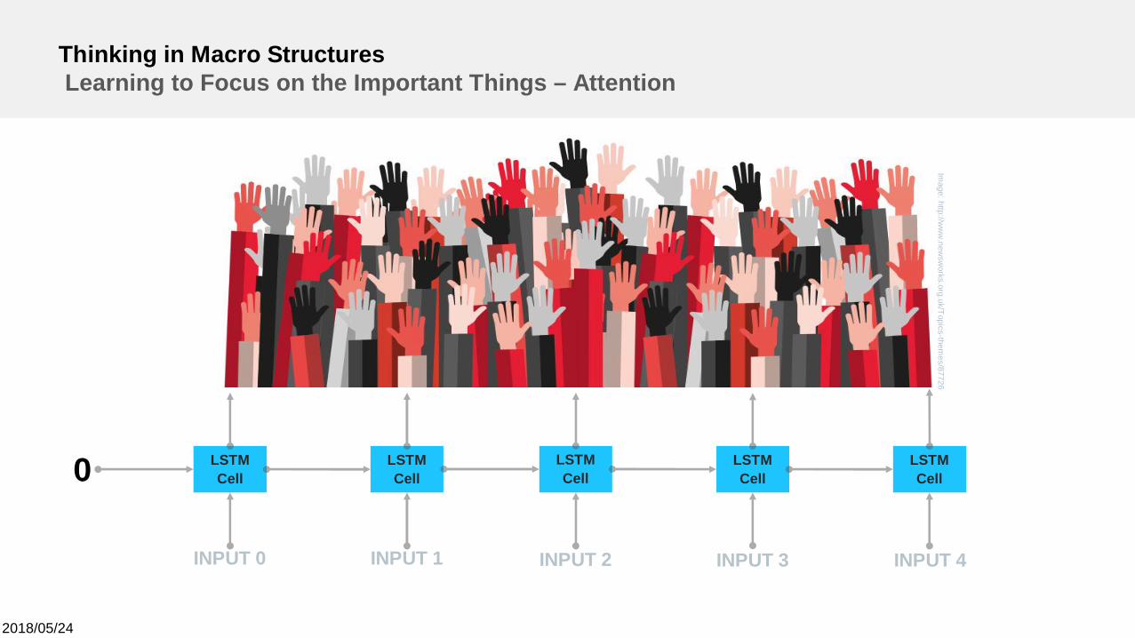
Thinking in Macro StructuresLearning to Focus on the Important Things – Attention
Image:http://w
ww
.newsw
orks.org.uk/Topics-themes/87726
LSTMCell
LSTMCell
LSTMCell
LSTMCell
LSTMCell0
INPUT 0 INPUT 1 INPUT 2 INPUT 3 INPUT 4
2018/05/24
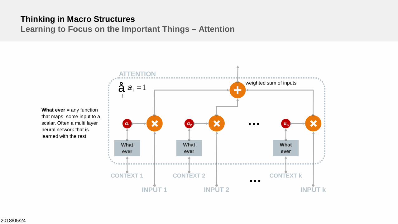
Thinking in Macro StructuresLearning to Focus on the Important Things – Attention
CONTEXT 1
ATTENTION
What ever = any functionthat maps some input to ascalar. Often a multi layerneural network that islearned with the rest.
INPUT 1
Whatever
α1
CONTEXT 2
INPUT 2
Whatever
α2
CONTEXT k
INPUT k
Whatever
αn
+
…
…
å =i
i 1aweighted sum of inputs
2018/05/24
Thinking in Macro StructuresLearning to Focus on the Important Things – Attention
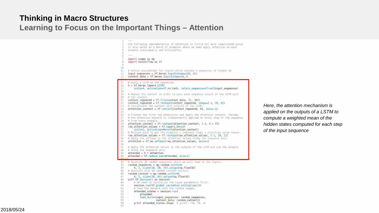
Here, the attention mechanism isapplied on the outputs of a LSTM tocompute a weighted mean of thehidden states computed for each stepof the input sequence
2018/05/24
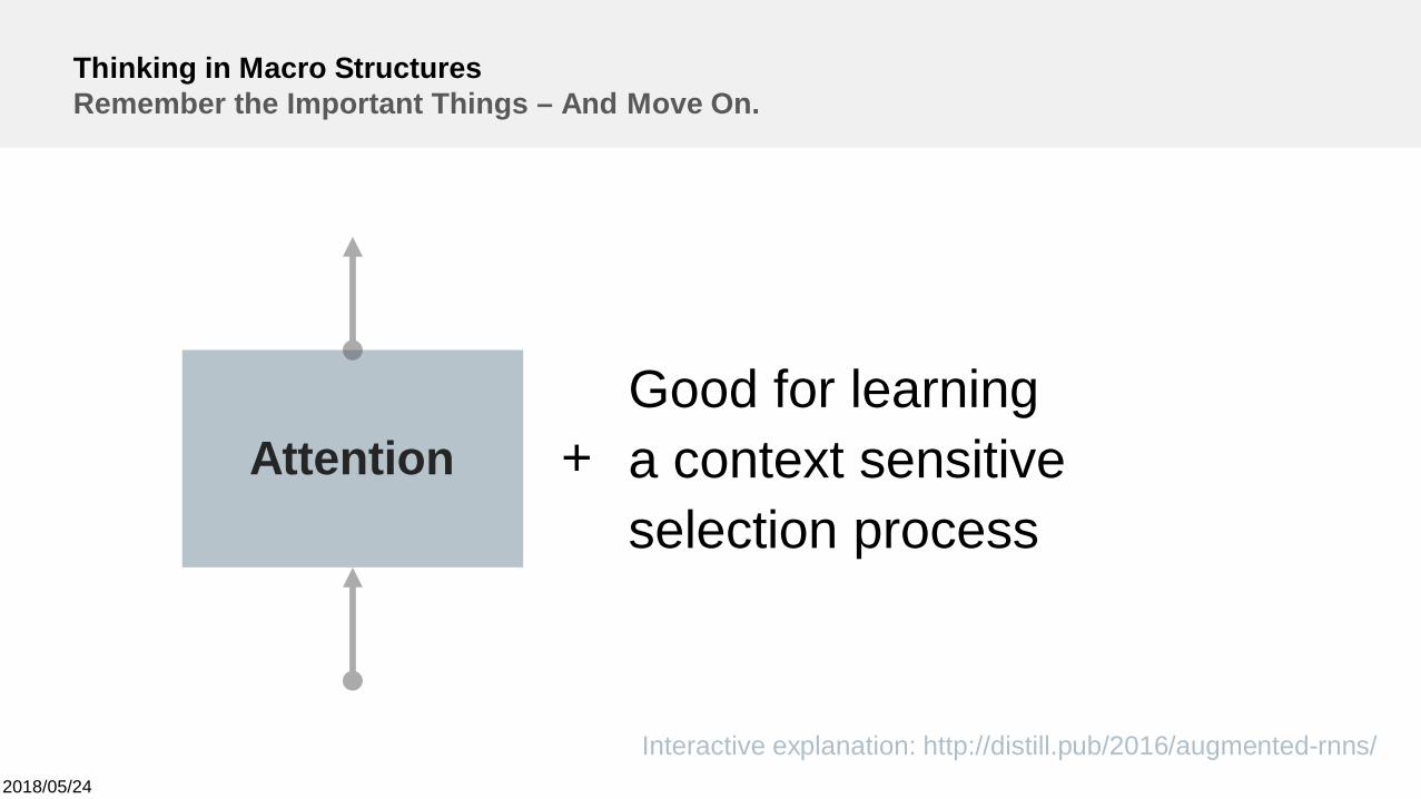
Thinking in Macro StructuresRemember the Important Things – And Move On.
AttentionGood for learninga context sensitiveselection process
+
Interactive explanation: http://distill.pub/2016/augmented-rnns/
2018/05/24
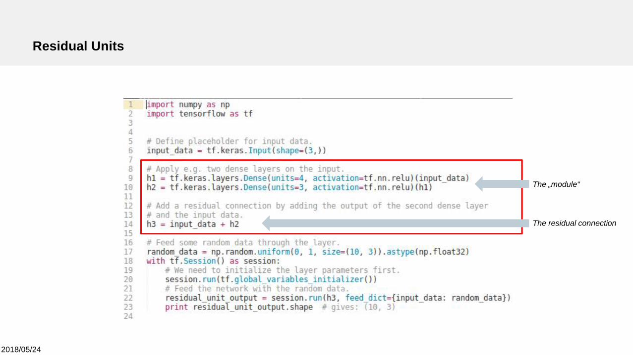
Residual Units
INPUT
Module
+OUTPUT
RES
IDU
ALC
ON
NEC
TIO
N
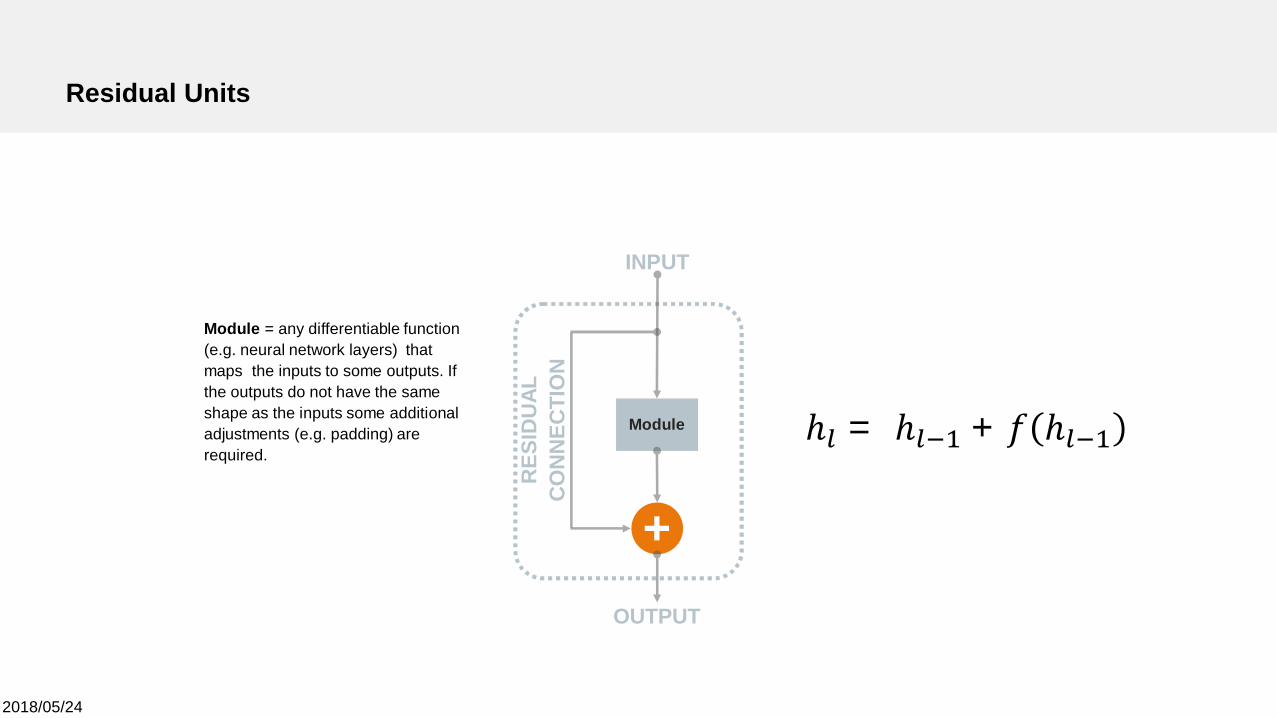
ℎ = ℎ + ℎ
Module = any differentiable function(e.g. neural network layers) thatmaps the inputs to some outputs. Ifthe outputs do not have the sameshape as the inputs some additionaladjustments (e.g. padding) arerequired.
2018/05/24
Residual Units
The „module“
The residual connection
2018/05/24
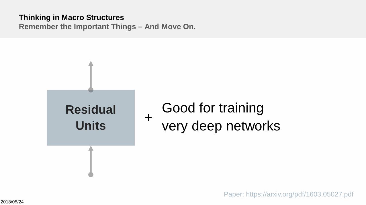
Thinking in Macro StructuresRemember the Important Things – And Move On.
ResidualUnits
Good for trainingvery deep networks+
Paper: https://arxiv.org/pdf/1603.05027.pdf

And more…
Deep LearningEnd-to-End Model Design
2018/05/24
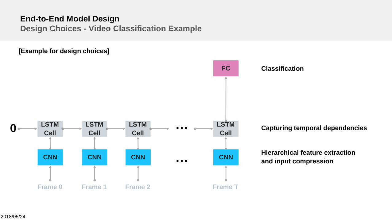
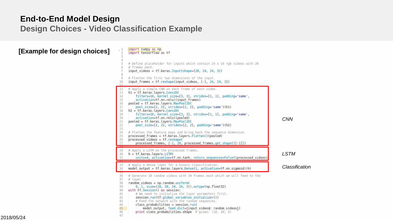
End-to-End Model DesignDesign Choices - Video Classification Example
0 LSTMCell
Frame 0
CNN
LSTMCell
Frame 1
CNN
LSTMCell
Frame 2
CNN
Frame T
LSTMCell
CNN
FC
…
… Hierarchical feature extractionand input compression
Capturing temporal dependencies
Classification
[Example for design choices]
2018/05/24
End-to-End Model DesignDesign Choices - Video Classification Example
[Example for design choices]
CNN
LSTM
Classification
2018/05/24
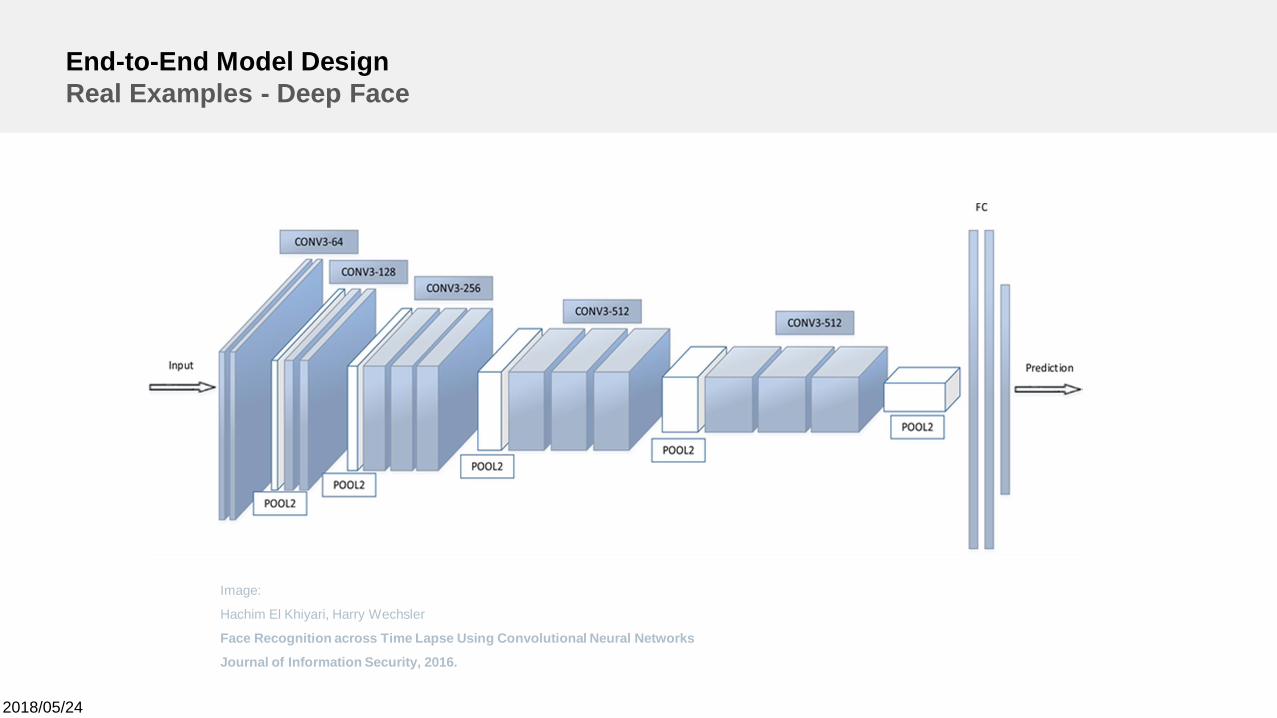
End-to-End Model DesignReal Examples - Deep Face
Image:
Hachim El Khiyari, Harry Wechsler
Face Recognition across Time Lapse Using Convolutional Neural Networks
Journal of Information Security, 2016.
2018/05/24
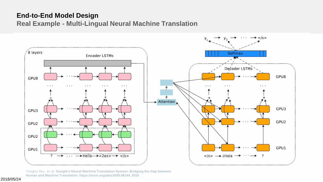
End-to-End Model DesignReal Example - Multi-Lingual Neural Machine Translation
Yonghui Wu, et. al. Google's Neural Machine Translation System: Bridging the Gap betweenHuman and Machine Translation. https://arxiv.org/abs/1609.08144. 2016
2018/05/24
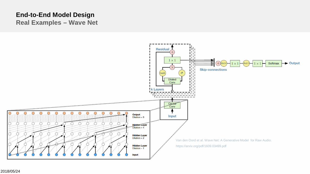
End-to-End Model DesignReal Examples – Wave Net
Van den Oord et al. Wave Net: A Generative Model for Raw Audio.
https://arxiv.org/pdf/1609.03499.pdf
Deep LearningDeep Learning Model Training
2018/05/24
Basic Implementation Overview
1. Prepare the data2. Design the model architecture3. Design the optimization goals4. Train5. Evaluate6. Deploy
2018/05/24
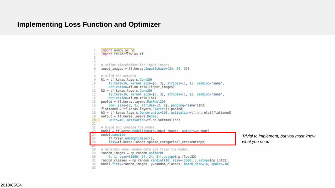
Implementing Loss Function and Optimizer
Trivial to implement, but you must knowwhat you need
2018/05/24
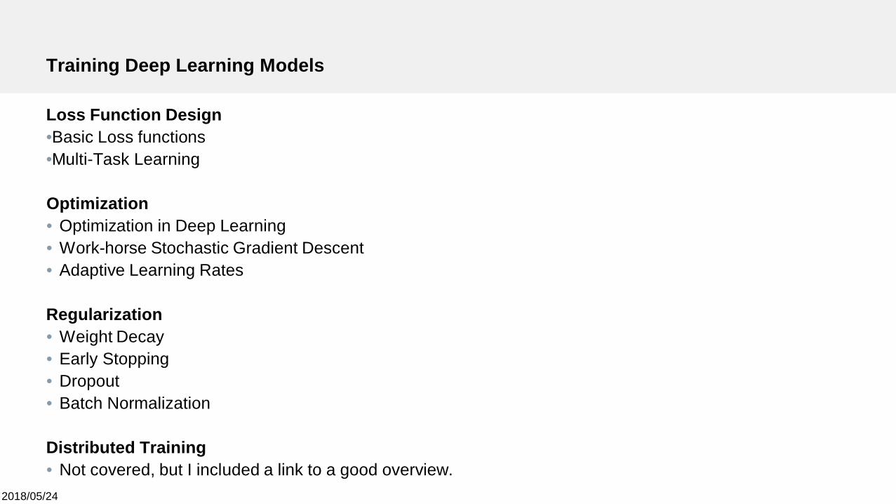
Training Deep Learning Models
Loss Function Design•Basic Loss functions•Multi-Task Learning
Optimization• Optimization in Deep Learning• Work-horse Stochastic Gradient Descent• Adaptive Learning Rates
Regularization• Weight Decay• Early Stopping• Dropout• Batch Normalization
Distributed Training• Not covered, but I included a link to a good overview.
Deep LearningLoss Function Design
2018/05/24
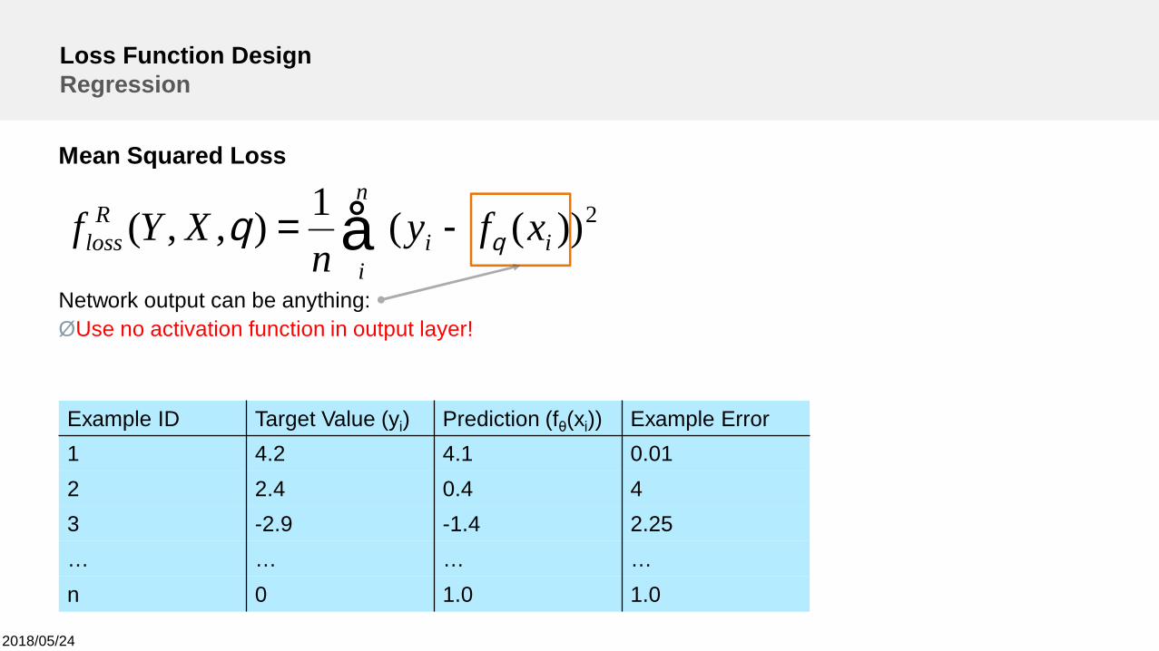
Loss Function DesignRegression
Mean Squared Loss
Network output can be anything:ØUse no activation function in output layer!
Example ID Target Value (yi) Prediction (fθ(xi)) Example Error1 4.2 4.1 0.012 2.4 0.4 43 -2.9 -1.4 2.25… … … …n 0 1.0 1.0
å -=n
iii
Rloss xfy
nXYf 2))((1),,( qq
2018/05/24
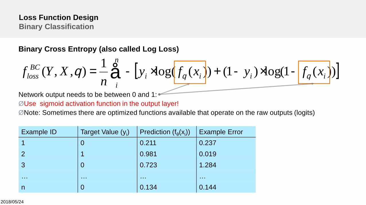
Loss Function DesignBinary Classification
Binary Cross Entropy (also called Log Loss)
Network output needs to be between 0 and 1:ØUse sigmoid activation function in the output layer!ØNote: Sometimes there are optimized functions available that operate on the raw outputs (logits)
[ ]å -×-+×-=n
iiiii
BCloss xfyxfy
nXYf ))(1(log)1())(log(1),,( qqq
Example ID Target Value (yi) Prediction (fθ(xi)) Example Error1 0 0.211 0.2372 1 0.981 0.0193 0 0.723 1.284… … … …n 0 0.134 0.144
2018/05/24
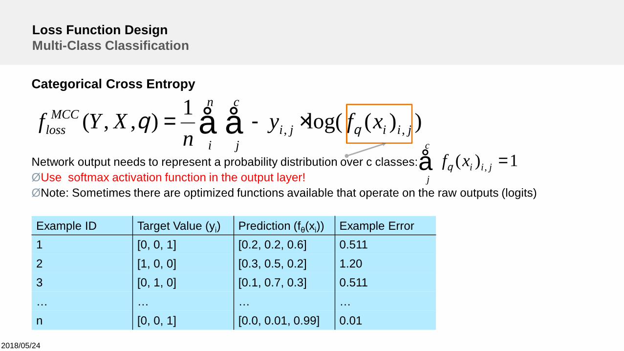
Categorical Cross Entropy
Network output needs to represent a probability distribution over c classes:ØUse softmax activation function in the output layer!ØNote: Sometimes there are optimized functions available that operate on the raw outputs (logits)
åå ×-=n
i
c
jjiiji
MCCloss xfy
nXYf ))(log(1),,( ,, qq
Loss Function DesignMulti-Class Classification
Example ID Target Value (yi) Prediction (fθ(xi)) Example Error1 [0, 0, 1] [0.2, 0.2, 0.6] 0.5112 [1, 0, 0] [0.3, 0.5, 0.2] 1.203 [0, 1, 0] [0.1, 0.7, 0.3] 0.511… … … …n [0, 0, 1] [0.0, 0.01, 0.99] 0.01
1)( , =åc
jjiixfq
2018/05/24
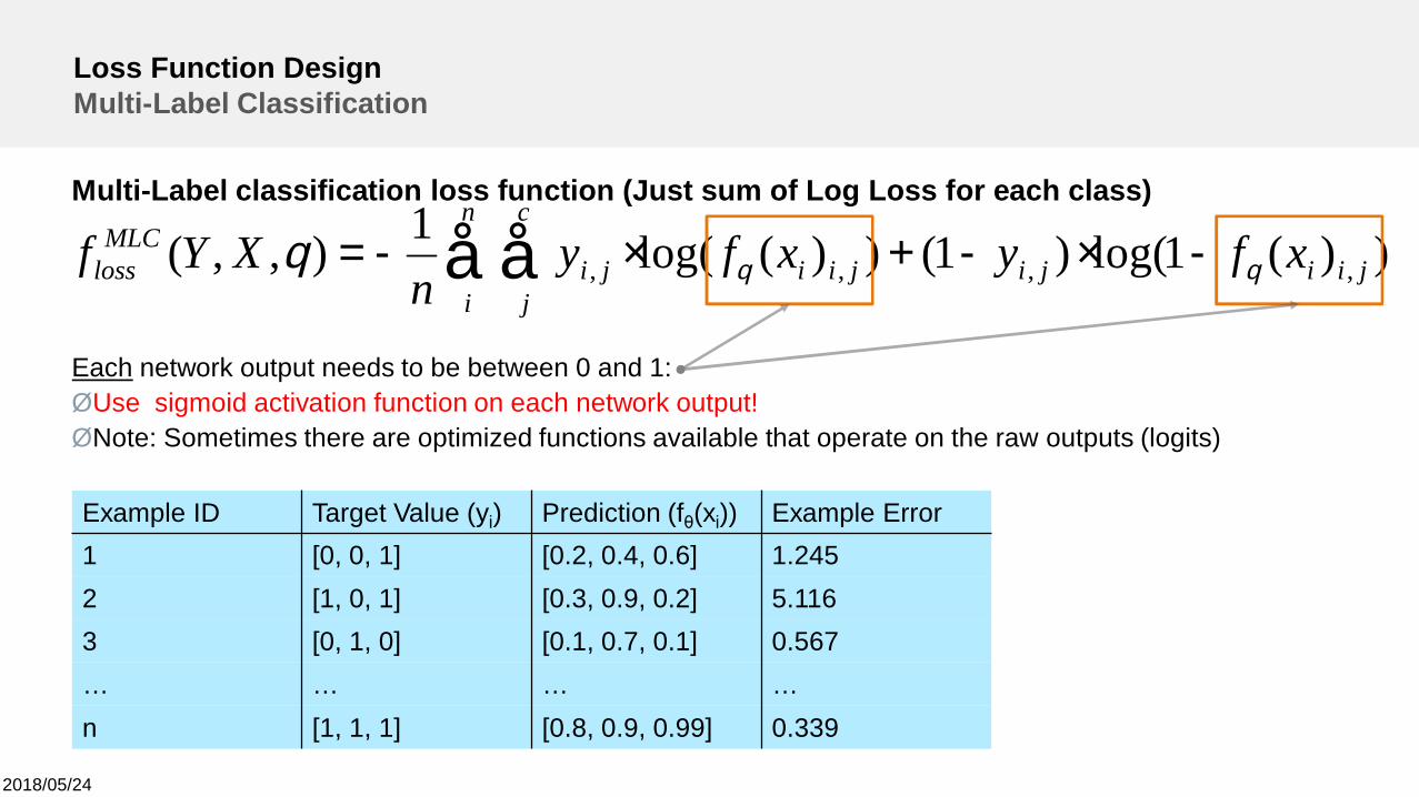
Multi-Label classification loss function (Just sum of Log Loss for each class)
Each network output needs to be between 0 and 1:ØUse sigmoid activation function on each network output!ØNote: Sometimes there are optimized functions available that operate on the raw outputs (logits)
))(1log()1())(log(1),,( ,,,, jiiji
n
i
c
jjiiji
MLCloss xfyxfy
nXYf qqq -×-+×-= åå
Loss Function DesignMulti-Label Classification
Example ID Target Value (yi) Prediction (fθ(xi)) Example Error1 [0, 0, 1] [0.2, 0.4, 0.6] 1.2452 [1, 0, 1] [0.3, 0.9, 0.2] 5.1163 [0, 1, 0] [0.1, 0.7, 0.1] 0.567… … … …n [1, 1, 1] [0.8, 0.9, 0.99] 0.339
2018/05/24
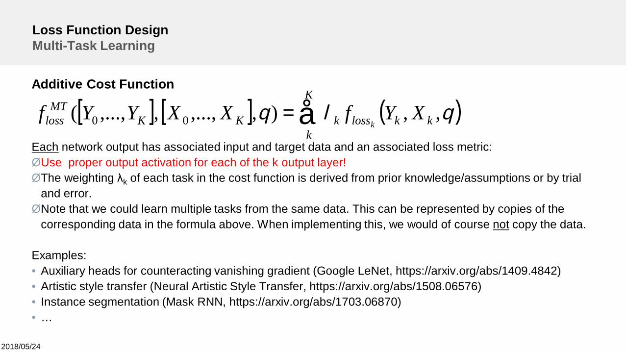
Additive Cost Function
Each network output has associated input and target data and an associated loss metric:ØUse proper output activation for each of the k output layer!ØThe weighting λk of each task in the cost function is derived from prior knowledge/assumptions or by trial
and error.ØNote that we could learn multiple tasks from the same data. This can be represented by copies of the
corresponding data in the formula above. When implementing this, we would of course not copy the data.
Examples:• Auxiliary heads for counteracting vanishing gradient (Google LeNet, https://arxiv.org/abs/1409.4842)• Artistic style transfer (Neural Artistic Style Transfer, https://arxiv.org/abs/1508.06576)• Instance segmentation (Mask RNN, https://arxiv.org/abs/1703.06870)• …
Loss Function DesignMulti-Task Learning
[ ] [ ] ( )qlq ,,),,...,,,...,( 00 kk
K
klosskKK
MTloss XYfXXYYf
kå=
Deep LearningOptimization
2018/05/24
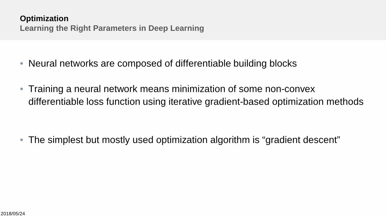
OptimizationLearning the Right Parameters in Deep Learning
• Neural networks are composed of differentiable building blocks
• Training a neural network means minimization of some non-convexdifferentiable loss function using iterative gradient-based optimization methods
• The simplest but mostly used optimization algorithm is “gradient descent”
2018/05/24
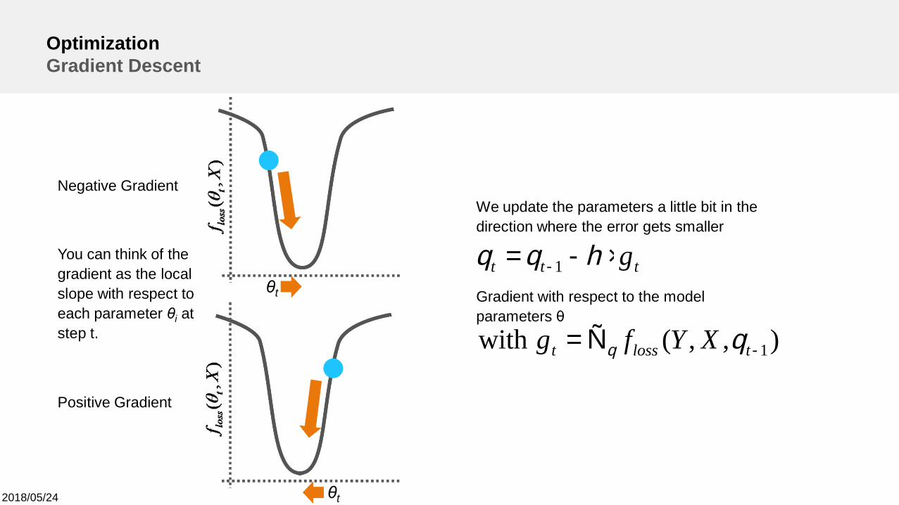
Gradient with respect to the modelparameters θ
),,(with 1
1
-
-
Ñ=
×-=
tlosst
ttt
XYfg
g
q
hqq
q
OptimizationGradient Descent
We update the parameters a little bit in thedirection where the error gets smaller
Negative Gradient
Positive Gradient
θt
θt
You can think of thegradient as the localslope with respect toeach parameter θi atstep t.
2018/05/24
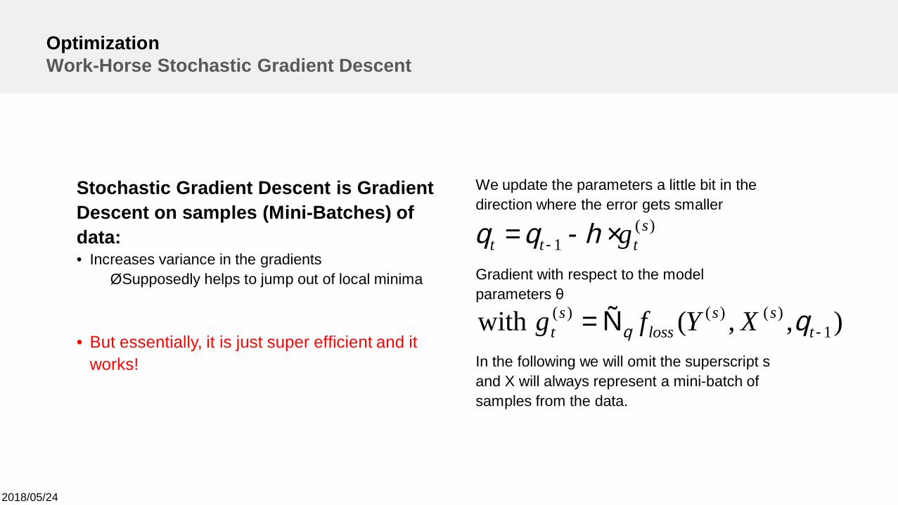
),,(with 1)()()(
)(1
-
-
Ñ=
×-=
tss
losss
t
sttt
XYfg
g
q
hqq
q
Gradient with respect to the modelparameters θ
OptimizationWork-Horse Stochastic Gradient Descent
We update the parameters a little bit in thedirection where the error gets smaller
Stochastic Gradient Descent is GradientDescent on samples (Mini-Batches) ofdata:• Increases variance in the gradients
ØSupposedly helps to jump out of local minima
• But essentially, it is just super efficient and itworks! In the following we will omit the superscript s
and X will always represent a mini-batch ofsamples from the data.
2018/05/24
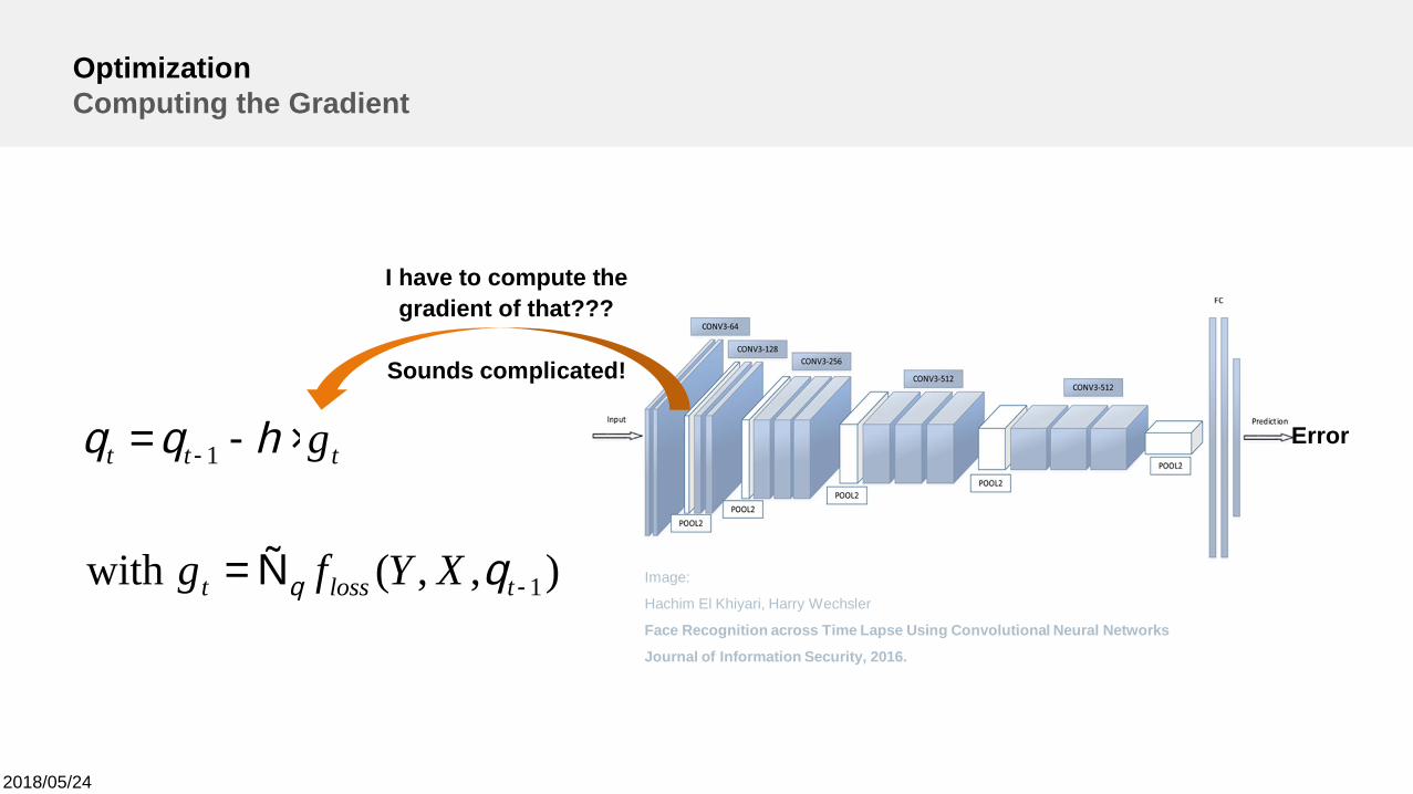
OptimizationComputing the Gradient
I have to compute thegradient of that???
Sounds complicated!
Error
),,(with 1
1
-
-
Ñ=
×-=
tlosst
ttt
XYfg
g
q
hqq
q Image:
Hachim El Khiyari, Harry Wechsler
Face Recognition across Time Lapse Using Convolutional Neural Networks
Journal of Information Security, 2016.
2018/05/24
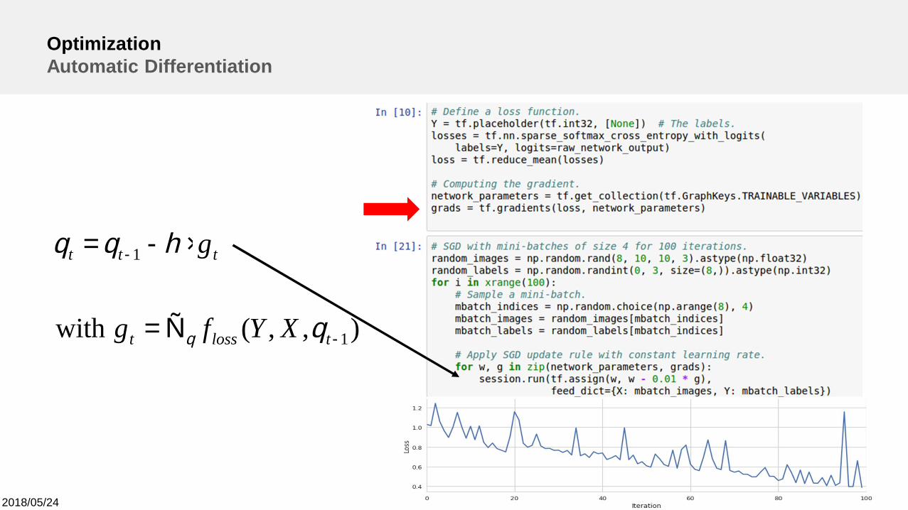
OptimizationAutomatic Differentiation
),,(with 1
1
-
-
Ñ=
×-=
tlosst
ttt
XYfg
g
q
hqq
q
2018/05/24
OptimizationAutomatic Differentiation
AUTOMATIC DIFFERENTIATIONIS AN
EXTREMELY POWERFUL FEATUREFOR DEVELOPING MODELS WITH
DIFFERENTIABLEOPTIMIZATION OBJECTIVES
2018/05/24
OptimizationWait a Minute, I thought Neural Networks are Optimized via Backpropagation
Backpropagation is just a fancy name forapplying the chain rule to compute the
gradients in neural networks!
2018/05/24
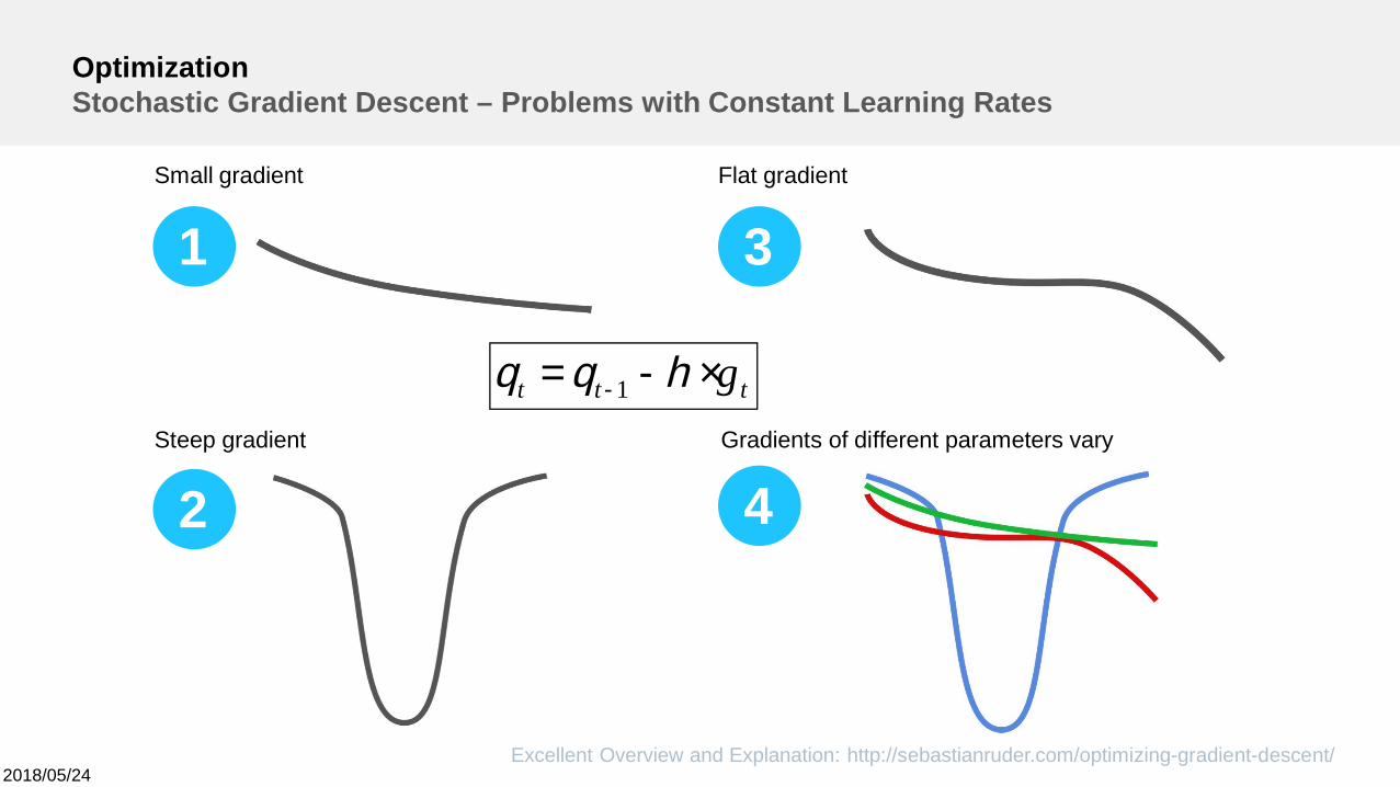
OptimizationStochastic Gradient Descent – Problems with Constant Learning Rates
Excellent Overview and Explanation: http://sebastianruder.com/optimizing-gradient-descent/
1
2
3
4
Small gradient
Steep gradient
Flat gradient
Gradients of different parameters vary
ttt g×-= - hqq 1
2018/05/24
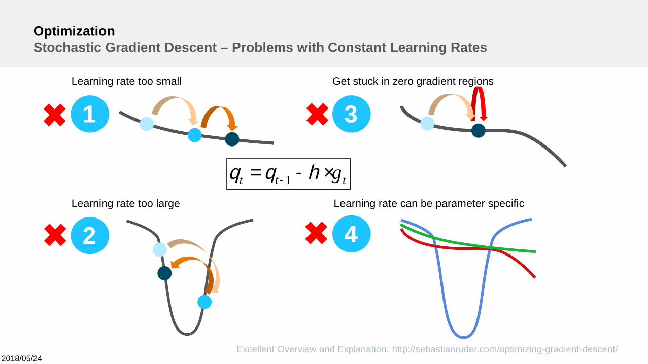
OptimizationStochastic Gradient Descent – Problems with Constant Learning Rates
Excellent Overview and Explanation: http://sebastianruder.com/optimizing-gradient-descent/
1
2
3
4
Learning rate too small
Learning rate too large
Get stuck in zero gradient regions
Learning rate can be parameter specific
ttt g×-= - hqq 1
2018/05/24
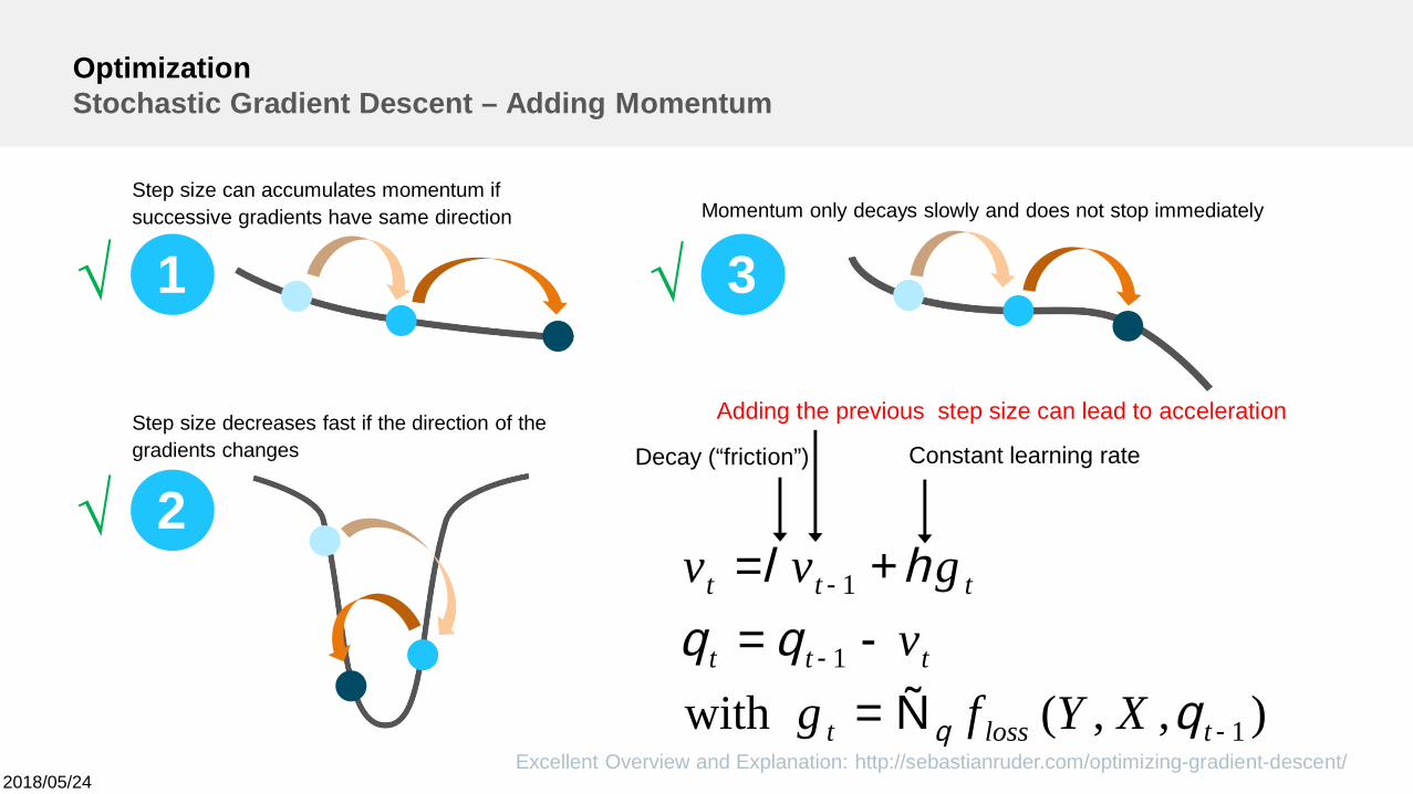
OptimizationStochastic Gradient Descent – Adding Momentum
Excellent Overview and Explanation: http://sebastianruder.com/optimizing-gradient-descent/
1
2
3
Step size can accumulates momentum ifsuccessive gradients have same direction
Step size decreases fast if the direction of thegradients changes
Momentum only decays slowly and does not stop immediately
),,(with 1
1
1
-
-
-
Ñ=-=+=
tlosst
ttt
ttt
XYfgv
gvv
qqq
hl
q
Decay (“friction”) Constant learning rate
Adding the previous step size can lead to acceleration
√
√
√
2018/05/24
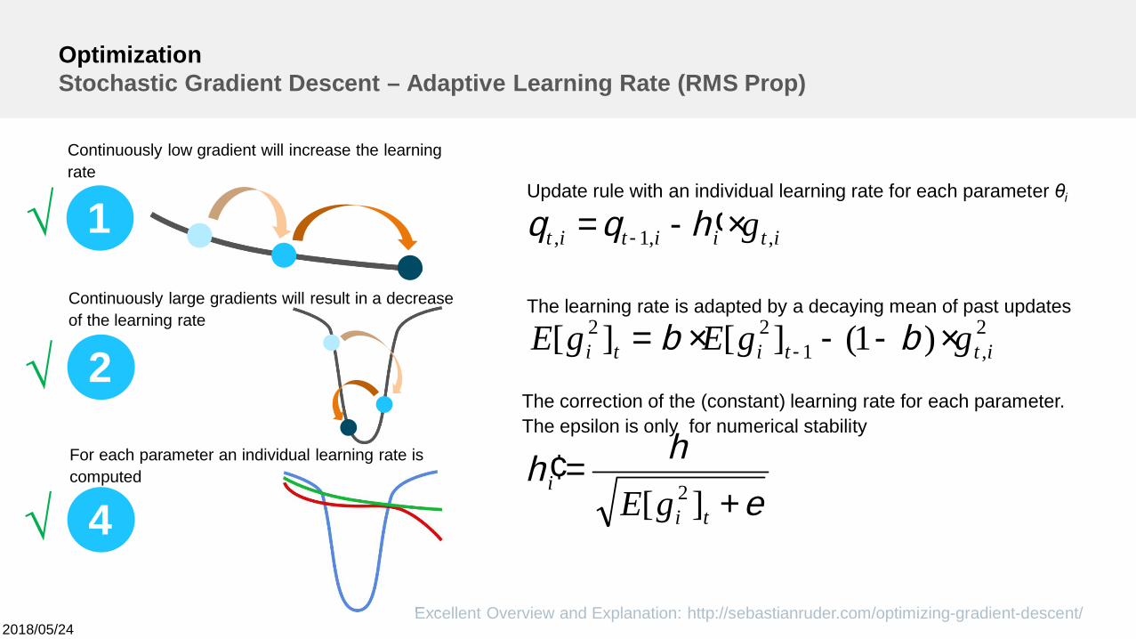
OptimizationStochastic Gradient Descent – Adaptive Learning Rate (RMS Prop)
Excellent Overview and Explanation: http://sebastianruder.com/optimizing-gradient-descent/
4For each parameter an individual learning rate iscomputed
e
hh
bb
hqq
+=¢
×--×=
×¢-=
-
-
ti
i
ittiti
itiitit
gE
ggEgE
g
][
)1(][][
2
2,1
22
,,1,
Update rule with an individual learning rate for each parameter θi
The learning rate is adapted by a decaying mean of past updates
The correction of the (constant) learning rate for each parameter.The epsilon is only for numerical stability
1
Continuously low gradient will increase the learningrate
2
Continuously large gradients will result in a decreaseof the learning rate
√
√
√
2018/05/24
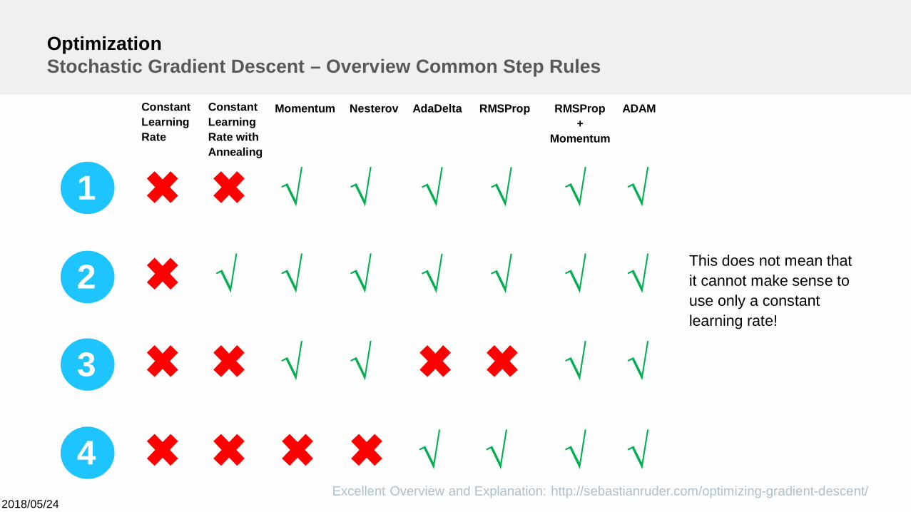
OptimizationStochastic Gradient Descent – Overview Common Step Rules
Excellent Overview and Explanation: http://sebastianruder.com/optimizing-gradient-descent/
1
2
3
4
ConstantLearningRate
ConstantLearningRate withAnnealing
Momentum AdaDelta RMSProp RMSProp+
Momentum
ADAMNesterov
√
√
√
√
√
√
√ √
√
√
√
√
√
√
√
√
This does not mean thatit cannot make sense touse only a constantlearning rate!
√
√
√
√
√
Deep LearningRegularization
2018/05/24
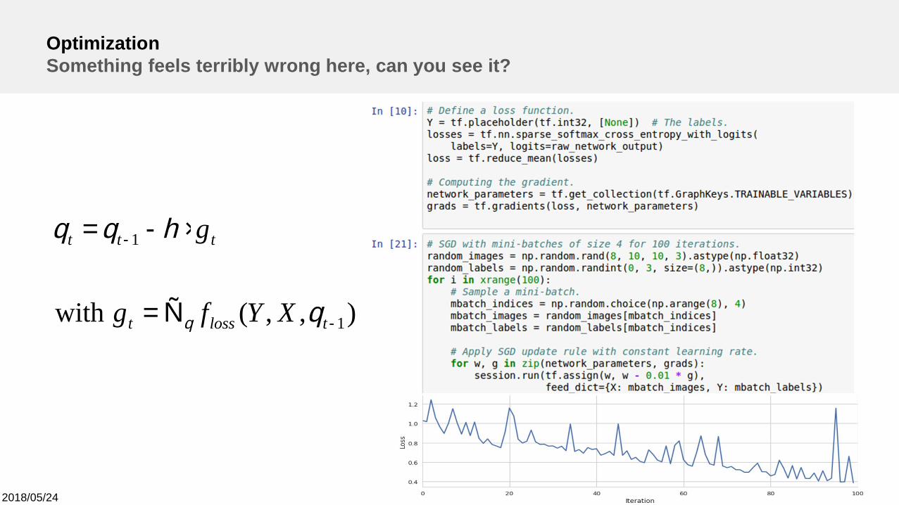
OptimizationSomething feels terribly wrong here, can you see it?
),,(with 1
1
-
-
Ñ=
×-=
tlosst
ttt
XYfg
g
q
hqq
q
2018/05/24
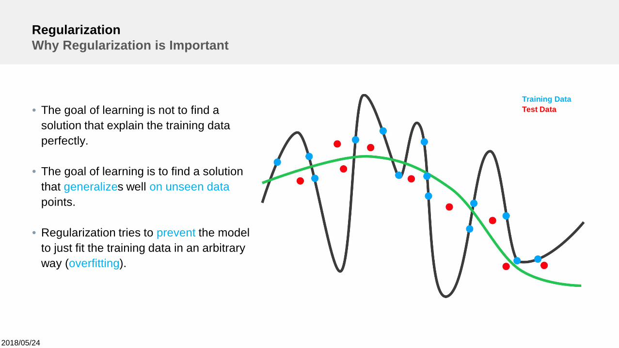
RegularizationWhy Regularization is Important
• The goal of learning is not to find asolution that explain the training dataperfectly.
• The goal of learning is to find a solutionthat generalizes well on unseen datapoints.
• Regularization tries to prevent the modelto just fit the training data in an arbitraryway (overfitting).
Training DataTest Data
2018/05/24
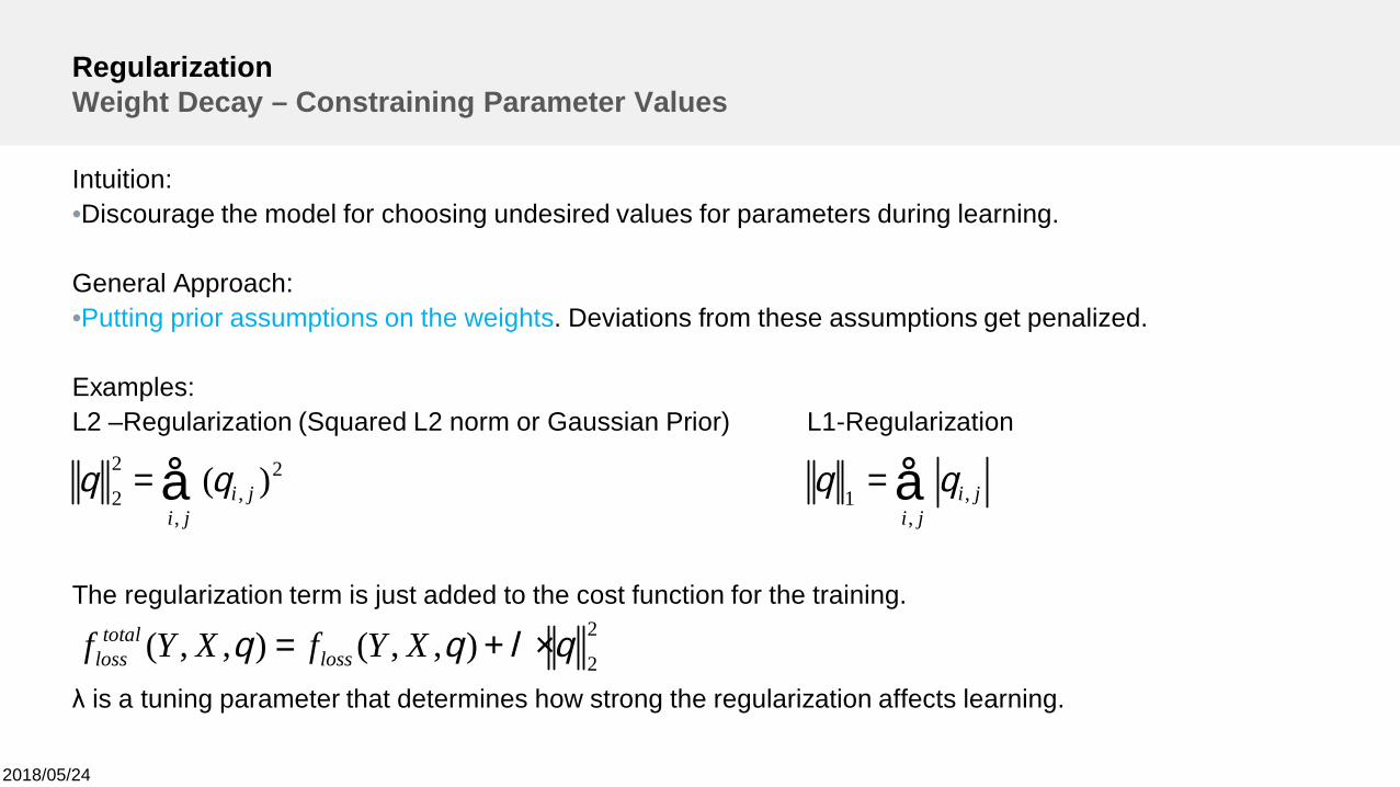
RegularizationWeight Decay – Constraining Parameter Values
Intuition:•Discourage the model for choosing undesired values for parameters during learning.
General Approach:•Putting prior assumptions on the weights. Deviations from these assumptions get penalized.
Examples:L2 –Regularization (Squared L2 norm or Gaussian Prior) L1-Regularization
The regularization term is just added to the cost function for the training.
λ is a tuning parameter that determines how strong the regularization affects learning.
å=ji
ji,
2,
2
2)(qq
2
2),,(),,( qlqq ×+= XYfXYf loss
totalloss
å=ji
ji,
,1qq
2018/05/24
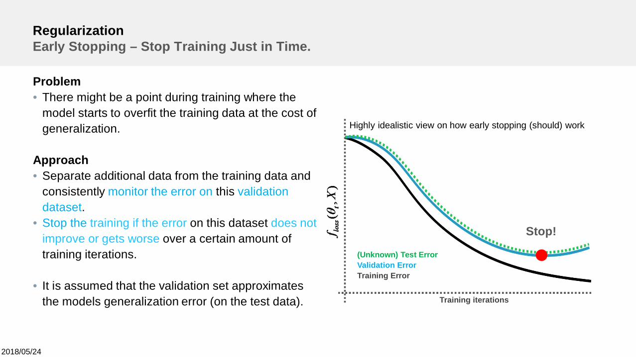
RegularizationEarly Stopping – Stop Training Just in Time.
Problem• There might be a point during training where the
model starts to overfit the training data at the cost ofgeneralization.
Approach• Separate additional data from the training data and
consistently monitor the error on this validationdataset.
• Stop the training if the error on this dataset does notimprove or gets worse over a certain amount oftraining iterations.
• It is assumed that the validation set approximatesthe models generalization error (on the test data).
Stop!
(Unknown) Test ErrorValidation ErrorTraining Error
Training iterations
Highly idealistic view on how early stopping (should) work
2018/05/24
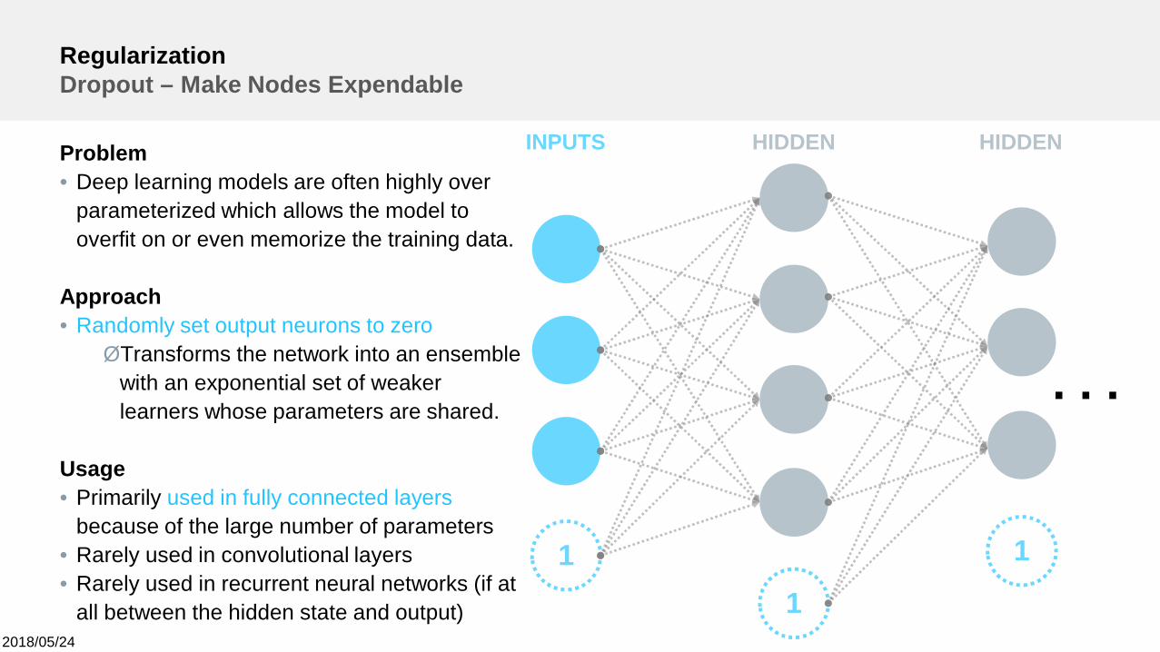
RegularizationDropout – Make Nodes Expendable
Problem• Deep learning models are often highly over
parameterized which allows the model tooverfit on or even memorize the training data.
Approach• Randomly set output neurons to zeroØTransforms the network into an ensemble
with an exponential set of weakerlearners whose parameters are shared.
Usage• Primarily used in fully connected layers
because of the large number of parameters• Rarely used in convolutional layers• Rarely used in recurrent neural networks (if at
all between the hidden state and output)
11
1
INPUTS HIDDEN HIDDEN
. . .
2018/05/24
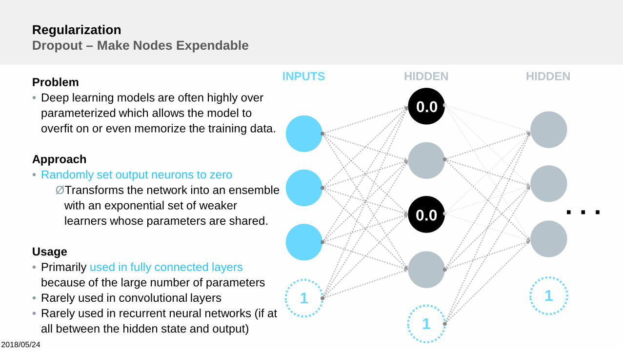
RegularizationDropout – Make Nodes Expendable
11
1
INPUTS HIDDEN HIDDEN
. . .
0.0
0.0
Problem• Deep learning models are often highly over
parameterized which allows the model tooverfit on or even memorize the training data.
Approach• Randomly set output neurons to zeroØTransforms the network into an ensemble
with an exponential set of weakerlearners whose parameters are shared.
Usage• Primarily used in fully connected layers
because of the large number of parameters• Rarely used in convolutional layers• Rarely used in recurrent neural networks (if at
all between the hidden state and output)
2018/05/24
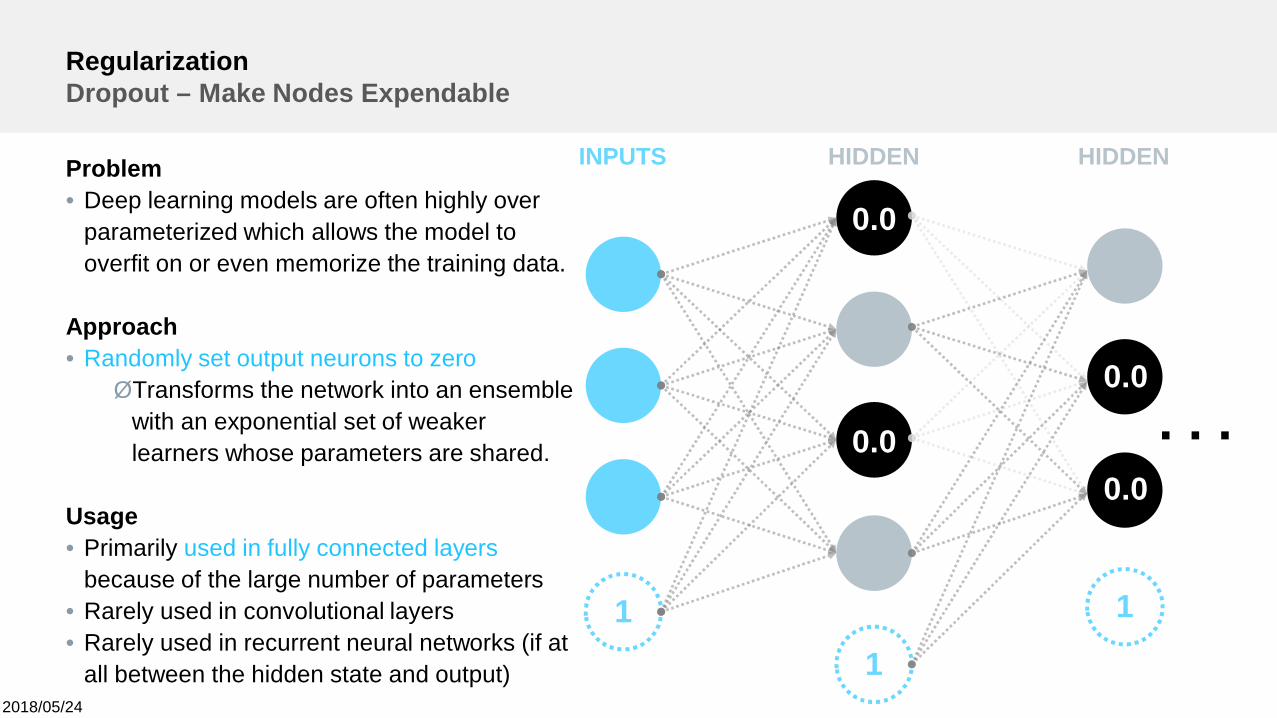
RegularizationDropout – Make Nodes Expendable
11
1
INPUTS HIDDEN HIDDEN
. . .
0.0
0.00.0
0.0
Problem• Deep learning models are often highly over
parameterized which allows the model tooverfit on or even memorize the training data.
Approach• Randomly set output neurons to zeroØTransforms the network into an ensemble
with an exponential set of weakerlearners whose parameters are shared.
Usage• Primarily used in fully connected layers
because of the large number of parameters• Rarely used in convolutional layers• Rarely used in recurrent neural networks (if at
all between the hidden state and output)
2018/05/24
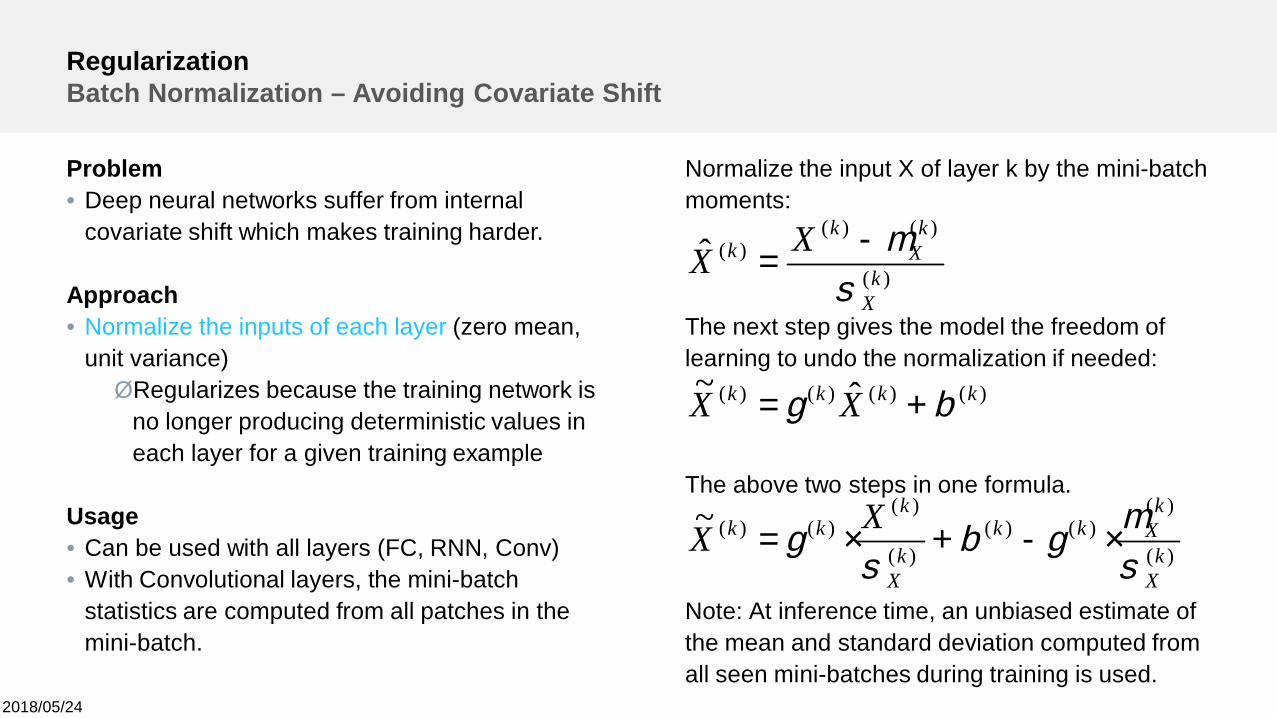
Normalize the input X of layer k by the mini-batchmoments:
The next step gives the model the freedom oflearning to undo the normalization if needed:
The above two steps in one formula.
Note: At inference time, an unbiased estimate ofthe mean and standard deviation computed fromall seen mini-batches during training is used.
)(
)()()(
)(
)()()(
)()()()(
)(
)()()(
~
ˆ~
ˆ
kX
kXkk
kX
kkk
kkkk
kX
kX
kk
XX
XX
XX
smgb
sg
bg
sm
×-+×=
+=
-=
RegularizationBatch Normalization – Avoiding Covariate Shift
Problem• Deep neural networks suffer from internal
covariate shift which makes training harder.
Approach• Normalize the inputs of each layer (zero mean,
unit variance)ØRegularizes because the training network is
no longer producing deterministic values ineach layer for a given training example
Usage• Can be used with all layers (FC, RNN, Conv)• With Convolutional layers, the mini-batch
statistics are computed from all patches in themini-batch.
Deep LearningAdditional Notes
2018/05/24
Distributed Training
https://blog.skymind.ai/distributed-deep-learning-part-1-an-introduction-to-distributed-training-of-neural-networks/
2018/05/24
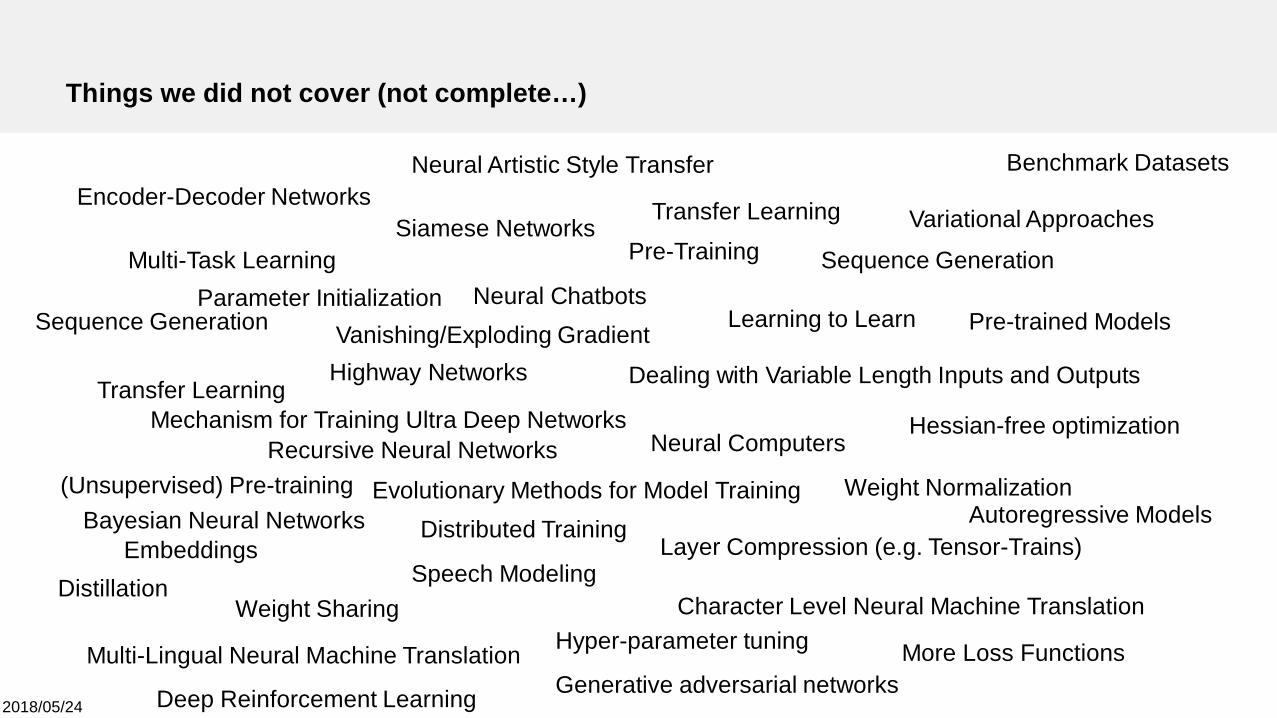
Things we did not cover (not complete…)
Encoder-Decoder Networks
Generative adversarial networks
Variational Approaches
Layer Compression (e.g. Tensor-Trains)
Evolutionary Methods for Model Training
Neural Computers
Dealing with Variable Length Inputs and Outputs
Pre-trained ModelsLearning to Learn
Transfer Learning
Siamese NetworksSequence Generation
Sequence Generation
Multi-Task Learning
Multi-Lingual Neural Machine Translation
Recursive Neural Networks
Character Level Neural Machine Translation
Neural Artistic Style Transfer
Neural Chatbots
Weight Normalization
Weight Sharing
(Unsupervised) Pre-training
Highway Networks
Transfer Learning
Speech Modeling
Vanishing/Exploding Gradient
Hessian-free optimization
More Loss FunctionsHyper-parameter tuning
Benchmark Datasets
Mechanism for Training Ultra Deep Networks
Parameter Initialization
Pre-Training
Distributed Training
Deep Reinforcement Learning
EmbeddingsDistillation
Bayesian Neural Networks Autoregressive Models
2018/05/24
Recommended Material
http://www.deeplearningbook.org/

2018/05/24
Recommended Courses
Deep Learning:
https://www.coursera.org/specializations/deep-learning#courses
Machine Learning
https://www.coursera.org/learn/machine-learning
Deep Learning:
There will be a lecture in WS 2018/2019

2018/05/24
Tackling AIchallenges
July 12th – 14th 2018Two major companies join forces to dive
deep into AI challenges together with you.
Join us for the AI Hackathon of theyear!
Featuring tracks on computer vision andimage recognition, digital companions,
natural language processing, signalprocessing, anomaly detection, and more.
Let’s develop something great together!
2018/05/24
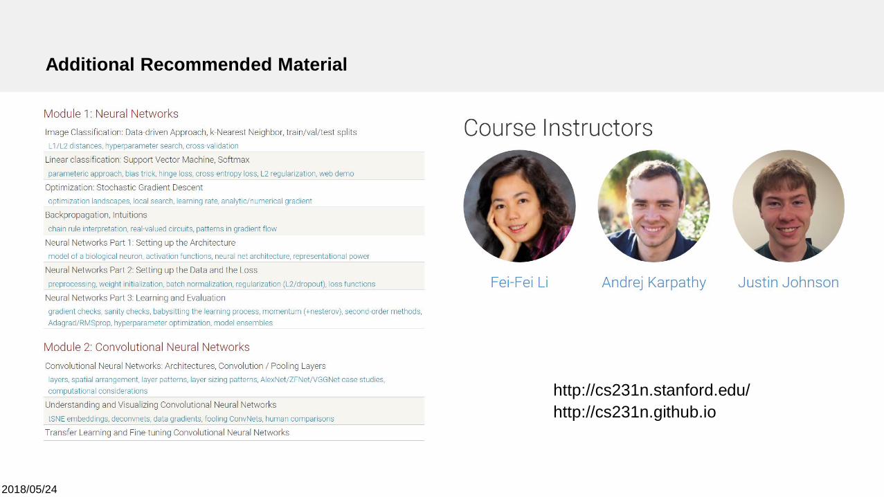
Additional Recommended Material
http://cs231n.stanford.edu/http://cs231n.github.io
2018/05/24
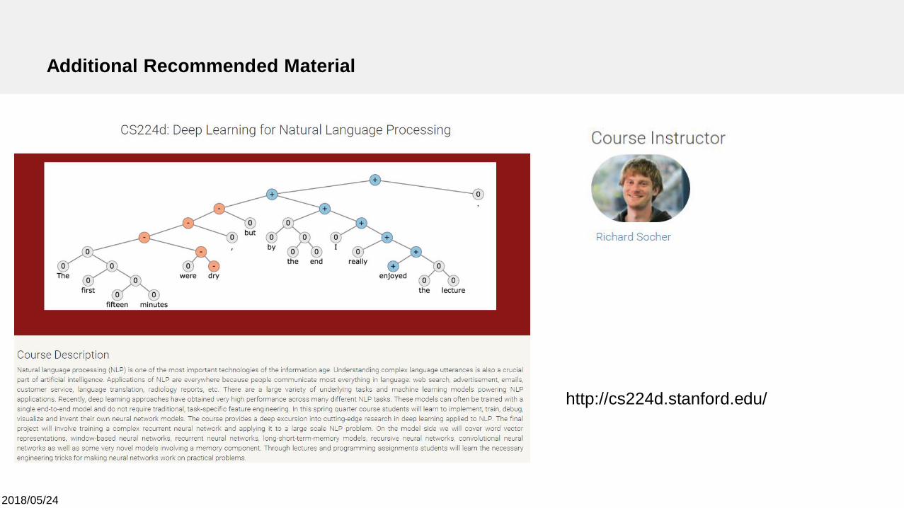
Additional Recommended Material
http://cs224d.stanford.edu/
2018/05/24
Additonal Recommended Material
INTRODUCTION• Tutorial on Neural Networks (Deep Learning and Unsupervised Feature
Learning): http://deeplearning.stanford.edu/wiki/index.php/UFLDL_Tutorial• Deep Learning for Computer Vision lecture: http://cs231n.stanford.edu (http://cs231n.github.io)• Deep Learning for NLP lecture: http://cs224d.stanford.edu (http://cs224d.stanford.edu/syllabus.html)• Deep Learning for NLP (without magic) tutorial: http://lxmls.it.pt/2014/socher-lxmls.pdf (Videos from NAACL
2013: http://nlp.stanford.edu/courses/NAACL2013)
2018/05/24
Additional Recommended Material
PARAMETER INITIALIZATION• Glorot, Xavier, and Yoshua Bengio. "Understanding the difficulty of training deep feedforward neural
networks." International Conference on Artificial Intelligence and Statistics. 2010.• He, K., Zhang, X., Ren, S., & Sun, J. (2015). Delving deep into rectifiers: Surpassing human-level performance on
ImageNet classification. In Proceedings of the IEEE International Conference on Computer Vision (pp. 1026-1034).
BATCH NORMALIZATION• Ioffe, S., & Szegedy, C. (2015). Batch Normalization: Accelerating Deep Network Training by Reducing Internal
Covariate Shift. In Proceedings of The 32nd International Conference on Machine Learning (pp. 448-456).• Cooijmans, T., Ballas, N., Laurent, C., & Courville, A. (2016). Recurrent Batch Normalization. arXiv preprint
arXiv:1603.09025.
DROPOUT• Hinton, Geoffrey E., et al. "Improving neural networks by preventing co-adaptation of feature detectors." arXiv preprint
arXiv:1207.0580 (2012).• Srivastava, Nitish, et al. "Dropout: A simple way to prevent neural networks from overfitting." The Journal of Machine
Learning Research 15.1 (2014): 1929-1958.
2018/05/24
Additional Recommended Material
OPTIMIZATION & TRAINING• Duchi, J., Hazan, E., & Singer, Y. (2011). Adaptive subgradient methods for online learning and stochastic
optimization. The Journal of Machine Learning Research, 12, 2121-2159.• Zeiler, M. D. (2012). ADADELTA: An adaptive learning rate method. arXiv preprint arXiv:1212.5701.• Tieleman, T., & Hinton, G. (2012). Lecture 6.5-rmsprop: Divide the gradient by a running average of its recent
magnitude. COURSERA: Neural Networks for Machine Learning, 4, 2.• Sutskever, I., Martens, J., Dahl, G., & Hinton, G. (2013). On the importance of initialization and momentum in deep
learning. In Proceedings of the 30th International Conference on Machine Learning (ICML) (pp. 1139-1147).• Kingma, D., & Ba, J. (2014). Adam: A method for stochastic optimization.arXiv preprint arXiv:1412.6980.• Martens, J., & Sutskever, I. (2012). Training deep and recurrent networks with hessian-free optimization. In Neural
networks: Tricks of the trade (pp. 479-535). Springer Berlin Heidelberg.
2018/05/24
Additional Recommended Material
COMPUTER VISION• Krizhevsky, A., Sutskever, I., & Hinton, G. E. (2012). ImageNet classification with deep convolutional neural networks.
In Advances in Neural Information Processing Systems (pp. 1097-1105).• Taigman, Y., Yang, M., Ranzato, M. A., & Wolf, L. (2014). DeepFace: Closing the gap to human-level performance in
face verification. In Proceedings of the IEEE Conference on Computer Vision and Pattern Recognition (pp. 1701-1708).• Szegedy, C., Liu, W., Jia, Y., Sermanet, P., Reed, S., Anguelov, D., ... & Rabinovich, A. (2015). Going deeper with
convolutions. In Proceedings of the IEEE Conference on Computer Vision and Pattern Recognition (pp. 1-9).• Simonyan, K., & Zisserman, A. (2014). Very deep convolutional networks for large-scale image recognition. arXiv
preprint arXiv:1409.1556.• Jaderberg, M., Simonyan, K., & Zisserman, A. (2015). Spatial transformer networks. In Advances in Neural Information
Processing Systems (pp. 2008-2016).• Ren, S., He, K., Girshick, R., & Sun, J. (2015). Faster R-CNN: Towards real-time object detection with region proposal
networks. In Advances in Neural Information Processing Systems (pp. 91-99).• Xu, K., Ba, J., Kiros, R., Cho, K., Courville, A., Salakhudinov, R., ... & Bengio, Y. (2015). Show, Attend and Tell: Neural
Image Caption Generation with Visual Attention. In Proceedings of The 32nd International Conference on MachineLearning (pp. 2048-2057).
• Johnson, J., Karpathy, A., & Fei-Fei, L. (2015). DenseCap: Fully Convolutional Localization Networks for DenseCaptioning. arXiv preprint arXiv:1511.07571.
2018/05/24
Additional Recommended Material
NATURAL LANGUAGE PROCESSING• Bengio, Y., Schwenk, H., Senécal, J. S., Morin, F., & Gauvain, J. L. (2006). Neural probabilistic language models.
In Innovations in Machine Learning (pp. 137-186). Springer Berlin Heidelberg.• Collobert, R., Weston, J., Bottou, L., Karlen, M., Kavukcuoglu, K., & Kuksa, P. (2011). Natural language processing
(almost) from scratch. The Journal of Machine Learning Research, 12, 2493-2537.• Mikolov, T. (2012). Statistical language models based on neural networks (Doctoral dissertation, PhD thesis, Brno
University of Technology. 2012.)• Mikolov, T., Chen, K., Corrado, G., & Dean, J. (2013). Efficient estimation of word representations in vector space. arXiv
preprint arXiv:1301.3781.• Mikolov, T., Sutskever, I., Chen, K., Corrado, G. S., & Dean, J. (2013). Distributed representations of words and phrases
and their compositionality. In Advances in Neural Information Processing Systems (pp. 3111-3119).• Mikolov, T., Yih, W. T., & Zweig, G. (2013). Linguistic Regularities in Continuous Space Word Representations. In HLT-
NAACL (pp. 746-751).• Socher, R. (2014). Recursive Deep Learning for Natural Language Processing and Computer Vision (Doctoral
dissertation, Stanford University).• Cho, K., Van Merriënboer, B., Gulcehre, C., Bahdanau, D., Bougares, F., Schwenk, H., & Bengio, Y. (2014). Learning
phrase representations using RNN encoder-decoder for statistical machine translation. arXiv preprint arXiv:1406.1078.• Bahdanau, D., Cho, K., & Bengio, Y. (2014). Neural machine translation by jointly learning to align and translate. arXiv
preprint arXiv:1409.0473.