Universitat Politecnica de Catalunya

Universitat de Barcelona

Universitat Rovira i Virgili

Facultat d’Informetica de Barcelona

Deep Learning for Expression Recognition inImage Sequences

Daniel Natanael Garcıa Zapata

Supervisors:

Dr. Sergio Escalera

Dr. Gholamreza Anbarjafari

Submitted in part fulfilment of the requirements for the degree ofMaster of Science in Artificial Intelligence

April 2018

Abstract

Facial expressions convey lots of information, which can be used for identifying emotions.

These facial expressions vary in time when they are being performed. Recognition of certain

emotions is a very challenging task even for people. This thesis consists of using machine

learning algorithms for recognizing emotions in image sequences. It uses the state-of-the-art

deep learning on collected data for automatic analysis of emotions. Concretely, the thesis

presents a comparison of current state-of-the-art learning strategies that can handle spatio-

temporal data and adapt classical static approaches to deal with images sequences. Expanded

versions of CNN, 3DCNN, and Recurrent approaches are evaluated and compared in two public

datasets for universal emotion recognition, where the performances are shown, and pros and

cons are discussed.

i

Resumen

Las expresiones faciales transmiten mucha informacion, las cuales pueden ser usadas para iden-

tificar emociones. Estas expresiones faciales varıan en tiempo cuando son realizadas. Inclusive

para las personas el reconocimiento de ciertas emociones es una tarea muy desafiante. Esta

tesis consiste en utilizar algoritmos de aprendizaje automatico para reconocer emociones en

secuencia de imagenes. Usando estado del arte del aprendizaje profundo en datos recolectados

para analisis automtico de emociones. Concretamente, esta tesis presenta una comparativa del

estado del arte actual de estrategias de aprendizaje que pueden manejar datos espaciotempo-

rales y una adaptacion de los enfoques clasicos para imgenes estaticas. Versiones expandidas

de CNN, 3DCNN y recurrentes son evaluadas y comparadas en dos conjuntos de datos publicos

de reconocimiento universal de emociones y donde se discuten los pros y contras.

ii

Resum

Les expressions facials transmeten molta informacio, que es pot utilitzar per identificar les emo-

cions. Aquestes expressions facials varien en el temps en que s’estan realitzant. El reconeixe-

ment de certes emocions es una tasca molt complicada fins i tot per a les persones. Aquesta tesi

consisteix a utilitzar algoritmes d’aprenentatge automtic per reconeixer emocions en sequencies

d’imatges. Utilitza Deep Learning d’ultima generacio sobre les dades recopilades per a l’analisi

automatic de les emocions. Concretament, la tesi presenta una comparacio de les estrategies

d’aprenentatge d’avantguarda actuals que permeten manejar dades espaciotemporals i adaptar

els enfocaments estatics classics per a tractar les sequencies d’imatges. Les versions ampliades

de CNN, 3DCNN i enfocaments recurrents s’avaluen i es comparen en dos conjunts de dades

d’expressions de sequencia d’imatges publiques per al reconeixement universal de l’emocio, on

es mostren els resultats i es discuteixen els pros i els contres.

iii

Acknowledgements

I would first like to thank my thesis advisor Doctor Sergio Escalera at Universitat de Barcelona.

Prof. Escalera was always open and available whenever I ran into any trouble or had any

question. He guided me in the right direction and gave me all his support.

Also, I would like to thank my second thesis advisor Doctor Gholamreza Anbarjafari (Shahab)

of the Intelligent Computer Vision Research Group at University of Tartu.

Finally, I must express my very profound gratitude to my parents and family for providing me

with unfailing support. This accomplishment would not have been possible without them.

iv

To my parents.

v

Contents

Abstract i

Acknowledgements iii

1 Introduction 1

1.1 Motivation and Objectives . . . . . . . . . . . . . . . . . . . . . . . . . . . . . . 1

1.2 Contributions . . . . . . . . . . . . . . . . . . . . . . . . . . . . . . . . . . . . . 2

2 Related Work 3

2.1 Related Work . . . . . . . . . . . . . . . . . . . . . . . . . . . . . . . . . . . . . 3

2.1.1 RGB Emotion Recognition . . . . . . . . . . . . . . . . . . . . . . . . . . 5

2.1.2 Multi-modal Emotion Recognition . . . . . . . . . . . . . . . . . . . . . . 6

2.1.3 Deep Learning base Emotion Recognition from Still Images . . . . . . . . 7

2.1.4 Deep Learning base Emotion Recognition from Image Sequences . . . . . 9

3 Theoretical Framework 11

3.1 Artificial Neural Networks . . . . . . . . . . . . . . . . . . . . . . . . . . . . . . 11

3.1.1 Backpropagation and Stochastic Gradient Descent . . . . . . . . . . . . . 12

vi

3.1.2 Architecture of Neural Network . . . . . . . . . . . . . . . . . . . . . . . 12

3.1.3 Loss Function . . . . . . . . . . . . . . . . . . . . . . . . . . . . . . . . . 14

3.1.4 Adaptive Learning Methods . . . . . . . . . . . . . . . . . . . . . . . . . 17

3.1.5 Activation Functions . . . . . . . . . . . . . . . . . . . . . . . . . . . . . 21

3.1.6 Sigmoid . . . . . . . . . . . . . . . . . . . . . . . . . . . . . . . . . . . . 21

3.1.7 Tanh . . . . . . . . . . . . . . . . . . . . . . . . . . . . . . . . . . . . . . 22

3.1.8 Rectified Linear Units . . . . . . . . . . . . . . . . . . . . . . . . . . . . 23

3.2 Convolutional Neural Networks . . . . . . . . . . . . . . . . . . . . . . . . . . . 23

3.2.1 CNN Architecture . . . . . . . . . . . . . . . . . . . . . . . . . . . . . . 25

3.2.2 Convolutional Layer . . . . . . . . . . . . . . . . . . . . . . . . . . . . . 26

3.2.3 Fully-Connected Layer . . . . . . . . . . . . . . . . . . . . . . . . . . . . 28

3.2.4 Pooling Layer . . . . . . . . . . . . . . . . . . . . . . . . . . . . . . . . . 28

3.3 3D Convolutional Neural Networks . . . . . . . . . . . . . . . . . . . . . . . . . 29

3.4 Recurrent Neural Networks . . . . . . . . . . . . . . . . . . . . . . . . . . . . . . 30

3.5 Long Short-Term Memory . . . . . . . . . . . . . . . . . . . . . . . . . . . . . . 31

3.5.1 LSTM Architecture . . . . . . . . . . . . . . . . . . . . . . . . . . . . . . 31

3.6 Gated Recurrent Units . . . . . . . . . . . . . . . . . . . . . . . . . . . . . . . . 35

3.7 Reducing Overfitting . . . . . . . . . . . . . . . . . . . . . . . . . . . . . . . . . 36

3.7.1 L1/L2 Regularization . . . . . . . . . . . . . . . . . . . . . . . . . . . . . 36

3.7.2 Dropout . . . . . . . . . . . . . . . . . . . . . . . . . . . . . . . . . . . . 37

3.7.3 Data Augmentation . . . . . . . . . . . . . . . . . . . . . . . . . . . . . . 37

vii

3.8 Dimensionality Reduction . . . . . . . . . . . . . . . . . . . . . . . . . . . . . . 38

4 Deep Architectures 41

4.1 Convolutional Neural Networks . . . . . . . . . . . . . . . . . . . . . . . . . . . 41

4.2 3D Convolutional Network . . . . . . . . . . . . . . . . . . . . . . . . . . . . . . 43

4.3 Recurrent Neural Networks . . . . . . . . . . . . . . . . . . . . . . . . . . . . . . 44

4.3.1 CNN + LSTM . . . . . . . . . . . . . . . . . . . . . . . . . . . . . . . . 44

4.3.2 CNN + GRU . . . . . . . . . . . . . . . . . . . . . . . . . . . . . . . . . 45

5 Datasets 46

5.1 SASE-FE . . . . . . . . . . . . . . . . . . . . . . . . . . . . . . . . . . . . . . . 46

5.2 OULU-CASIA . . . . . . . . . . . . . . . . . . . . . . . . . . . . . . . . . . . . . 48

6 Setup 50

6.1 Pre-processing . . . . . . . . . . . . . . . . . . . . . . . . . . . . . . . . . . . . . 50

7 Experimental Results 52

7.1 SASE-FE Emotion Results . . . . . . . . . . . . . . . . . . . . . . . . . . . . . . 52

7.1.1 No Pre-Processing . . . . . . . . . . . . . . . . . . . . . . . . . . . . . . 52

7.1.2 Frontalization . . . . . . . . . . . . . . . . . . . . . . . . . . . . . . . . . 53

7.1.3 2-Stream CNN . . . . . . . . . . . . . . . . . . . . . . . . . . . . . . . . 54

7.2 SASE-FE Hidden Emotion Results . . . . . . . . . . . . . . . . . . . . . . . . . 55

7.2.1 Still Images Input . . . . . . . . . . . . . . . . . . . . . . . . . . . . . . . 55

7.2.2 Image Sequences Input . . . . . . . . . . . . . . . . . . . . . . . . . . . . 56

viii

7.3 OULU-CASIA Results . . . . . . . . . . . . . . . . . . . . . . . . . . . . . . . . 57

7.3.1 Still Images Input . . . . . . . . . . . . . . . . . . . . . . . . . . . . . . . 57

7.3.2 Image Sequence Input . . . . . . . . . . . . . . . . . . . . . . . . . . . . 58

7.4 Discussion . . . . . . . . . . . . . . . . . . . . . . . . . . . . . . . . . . . . . . . 59

8 Conclusion 64

8.0.1 Future Work . . . . . . . . . . . . . . . . . . . . . . . . . . . . . . . . . . 65

Bibliography 65

ix

List of Tables

4.1 CNN Parameters . . . . . . . . . . . . . . . . . . . . . . . . . . . . . . . . . . . 43

4.2 3D CNN Parameters . . . . . . . . . . . . . . . . . . . . . . . . . . . . . . . . . 44

4.3 CNN + RNN Parameters . . . . . . . . . . . . . . . . . . . . . . . . . . . . . . . 45

5.1 SASE-FE Dataset . . . . . . . . . . . . . . . . . . . . . . . . . . . . . . . . . . . 47

5.2 OULU-CASIA Dataset . . . . . . . . . . . . . . . . . . . . . . . . . . . . . . . . 49

7.1 Emotion No Pre-processing Test Accuracy . . . . . . . . . . . . . . . . . . . . . 53

7.2 Emotion Frontalization Test Accuracy . . . . . . . . . . . . . . . . . . . . . . . 53

7.3 Emotion Fuse-Stream Test Accuracy . . . . . . . . . . . . . . . . . . . . . . . . 54

7.4 CNNs Hidden Test Accuracy . . . . . . . . . . . . . . . . . . . . . . . . . . . . . 55

7.5 Temporal Hidden Test Accuracy . . . . . . . . . . . . . . . . . . . . . . . . . . . 57

7.6 Temporal Test Accuracy . . . . . . . . . . . . . . . . . . . . . . . . . . . . . . . 58

7.7 Temporal Test Accuracy . . . . . . . . . . . . . . . . . . . . . . . . . . . . . . . 59

7.8 Final Models Discussion Accuracy . . . . . . . . . . . . . . . . . . . . . . . . . . 60

7.9 OULU-CASIA CNN Confusion Matrix . . . . . . . . . . . . . . . . . . . . . . . 60

7.10 OULU-CASIA CNN+Geometry Confusion Matrix . . . . . . . . . . . . . . . . . 61

x

List of Figures

2.1 Facial expression samples from JAFFE [35] database. (from [50]) . . . . . . . . 4

2.2 The images on the top level are from the original CK database and those on the

bottom are from the CK+ database. Both dataset present 7 emotions and 30

AUs. (from [34]) . . . . . . . . . . . . . . . . . . . . . . . . . . . . . . . . . . . 5

2.3 The face is tracked using an AAM to obtain features which are used for classifi-

cation using a linear SVM. . . . . . . . . . . . . . . . . . . . . . . . . . . . . . 5

2.4 Sample facial images with AU. (from [36]) . . . . . . . . . . . . . . . . . . . . . 6

2.5 Visual and Infrared image of a subject side by side. . . . . . . . . . . . . . . . . 7

2.6 Overview of the model proposed by Liu et al. (from [33]) . . . . . . . . . . . . 7

2.7 Example of a surprise emotion in emoFBVP dataset. (from [44]) . . . . . . . . 8

2.8 Participant of the KDEF database showing the emotions: angry, disgust, fear,

happy, neutral, sad and surprise. (from [2]) . . . . . . . . . . . . . . . . . . . . 9

2.9 SCAE architecture. . . . . . . . . . . . . . . . . . . . . . . . . . . . . . . . . . 9

2.10 Example of the region of interest image obtained while performing face land-

marks. (from [45]) . . . . . . . . . . . . . . . . . . . . . . . . . . . . . . . . . . 10

2.11 The hybrid CNN-RNN model proposed by Ronghen et al. (from [45]) . . . . . . 10

3.1 Typical architecture of an Artificial Neural Network. All layers are FC (from [54]) 14

xi

3.2 A single neuron schema.[24] . . . . . . . . . . . . . . . . . . . . . . . . . . . . . 14

3.3 The error is the difference between the real value y (red dots) and the predicted

values y (values in the function). [13] . . . . . . . . . . . . . . . . . . . . . . . . 15

3.4 Sigmoid activation function. . . . . . . . . . . . . . . . . . . . . . . . . . . . . . 21

3.5 Tanh activation function. . . . . . . . . . . . . . . . . . . . . . . . . . . . . . . . 22

3.6 ReLu activation function. . . . . . . . . . . . . . . . . . . . . . . . . . . . . . . 23

3.7 LeNet 5 . . . . . . . . . . . . . . . . . . . . . . . . . . . . . . . . . . . . . . . . 24

3.8 Alexnet Architecture . . . . . . . . . . . . . . . . . . . . . . . . . . . . . . . . . 24

3.9 Example of an image as a CNN input (from [51]) . . . . . . . . . . . . . . . . . 26

3.10 The weights and the window are described by the convolution kernel. . . . . . . 27

3.11 Left: Different from a FFNN, there are multiple neurons along the depth, all

looking at the same region in the input. Right: The neurons as with an FFNN,

computes a dot product but their connectivity is now restricted to be local

spatially (from [25]) . . . . . . . . . . . . . . . . . . . . . . . . . . . . . . . . . 27

3.12 Left: The example shows the input volume of size [224× 224× 64] is pooled into

a volume of size [112× 112× 64]. Right: Max pooling example using a stride of

2 (from [25]) . . . . . . . . . . . . . . . . . . . . . . . . . . . . . . . . . . . . . 29

3.13 Differences between a 2D CNN, 2D CNN with multiple frames and a 3D CNN

(from [57]) . . . . . . . . . . . . . . . . . . . . . . . . . . . . . . . . . . . . . . 29

3.14 The 3D kernel is applied in the input video to extract temporal features (from

[57]) . . . . . . . . . . . . . . . . . . . . . . . . . . . . . . . . . . . . . . . . . . 30

3.15 LSTM memory cell and control gates (from [41]) . . . . . . . . . . . . . . . . . 31

3.16 The cell state is the line that crosses the top of the memory cell (from [41]) . . 32

xii

3.17 Forget Gate. (from [57]) . . . . . . . . . . . . . . . . . . . . . . . . . . . . . . . 32

3.18 Input Gate. (from [57]) . . . . . . . . . . . . . . . . . . . . . . . . . . . . . . . 33

3.19 Update Gate (from [57]) . . . . . . . . . . . . . . . . . . . . . . . . . . . . . . . 34

3.20 Forget Gate (from [57]) . . . . . . . . . . . . . . . . . . . . . . . . . . . . . . . 34

3.21 Gated Recurrent Units Architecture. [41] . . . . . . . . . . . . . . . . . . . . . 35

3.22 Left: A standard neural net with 2 hidden layers. Right: An example of a

thinned net produced by applying dropout to the network on the left. (from [55]) 37

3.23 Style Data Augmentation Example (from [61]) . . . . . . . . . . . . . . . . . . . 38

3.24 Orientation Data Augmentation Example (from [61]) . . . . . . . . . . . . . . . 38

3.25 Colour Data Augmentation Example (from [61]) . . . . . . . . . . . . . . . . . . 38

3.26 The largest principal component is the direction that maximizes the variance

of the projected data, and the smallest principal component minimizes that

variance (from [14]) . . . . . . . . . . . . . . . . . . . . . . . . . . . . . . . . . 39

4.1 VGG-Face Architecture . . . . . . . . . . . . . . . . . . . . . . . . . . . . . . . . 42

4.2 Fully connected layers are listed as convolutional layers. Each convolution has

it’s corresponding padding, number of filters and stride (from [43]) . . . . . . . 42

4.3 C3D Architecture (from [57]) . . . . . . . . . . . . . . . . . . . . . . . . . . . . 43

5.1 Genuine and Deceptive emotions example in Fake vs Real Expressions dataset. 47

5.2 Six universal emotions example in Fake vs Real Expressions dataset. . . . . . . 48

5.3 Six universal emotions example in the OULU-CASIA dataset. . . . . . . . . . . 49

6.1 Right image shows an image with No Symmetry frontalization. Left image cor-

responds to a Soft Symmetry frontalization process. . . . . . . . . . . . . . . . . 51

xiii

6.2 68 fiducial points overlaid on the detected face. . . . . . . . . . . . . . . . . . . 51

7.1 Example of wrong and correct predicted images. . . . . . . . . . . . . . . . . . 62

xiv

Chapter 1

Introduction

1.1 Motivation and Objectives

The face of humans contains lots of information, some of this is useful to convey the emotion

that the person is transmitting. Emotion recognition in faces consists of a series of facial

expressions. In order to accurately recognise emotions, the whole range of these expressions

must be considered. Thus, it is important to consider image sequences where the full range of

the emotion is presented.

Emotion recognition is a complex task that even some humans have a hard time recognizing

certain emotions. Such is the case of blocked and/or micro emotions, a skilled person can

conceal an emotion that is being expressed with facial expressions. Unfortunately, common

people cannot accurately recognize real and fake facial expressions.

Deep Learning algorithms have gotten great results in the area of computer vision in identifying

human expressions, postures, etc. Recent advances have included a sequence of images that

represent the whole facial expression of the emotion from start to finish. This thesis presents a

comparison of computer vision techniques that seeks to recognise emotions in facial expressions

from image sequences. The comparison includes still images models and image sequences models

in the datasets. In addition, it extends to deep learning models with different inputs. The

1

objective of this comparison is to identify pros and cons of the different deep learning models

that are tested.

1.2 Contributions

This thesis tests state-of-the-art deep learning models for emotion recognition using two public

datasets.

• Pre-process emotion image sequences data to detect and align faces by means of rigid

registration.

• Consider different data modalities as features: face landmarks (i.e. geometry of the face),

CNN features on the face itself (spatial features), and 3DCNN features (spatio-temporal

ones).

• Evaluate the different feature modalities on current state-of-the-art deep models, i.e.

CNN, 3DCNN, and deep recurrent approaches.

• Evaluation of the methodology on two public emotion datasets analysing pros and cons

of the different methodologies.

2

Chapter 2

Related Work

2.1 Related Work

Facial expressions have an important role in human communication, specially about trans-

mitting emotions. With the crescent development of computer vision techniques in artificial

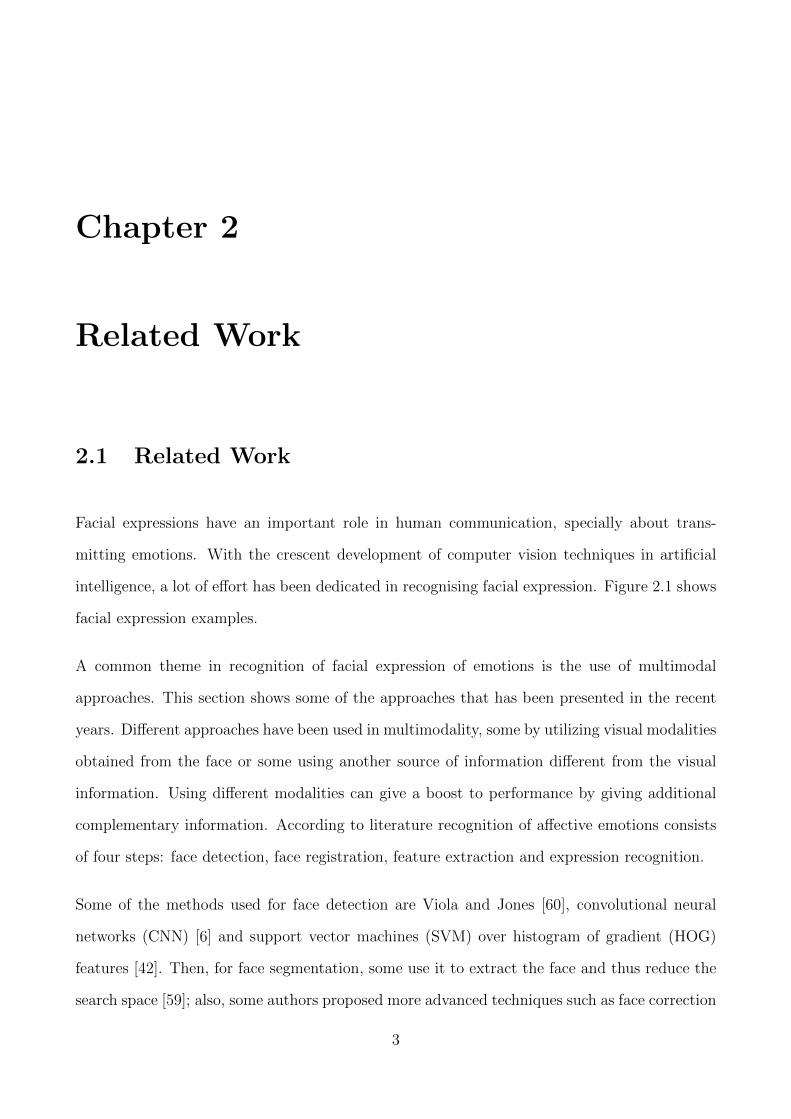
intelligence, a lot of effort has been dedicated in recognising facial expression. Figure 2.1 shows

facial expression examples.

A common theme in recognition of facial expression of emotions is the use of multimodal

approaches. This section shows some of the approaches that has been presented in the recent

years. Different approaches have been used in multimodality, some by utilizing visual modalities

obtained from the face or some using another source of information different from the visual

information. Using different modalities can give a boost to performance by giving additional

complementary information. According to literature recognition of affective emotions consists

of four steps: face detection, face registration, feature extraction and expression recognition.

Some of the methods used for face detection are Viola and Jones [60], convolutional neural

networks (CNN) [6] and support vector machines (SVM) over histogram of gradient (HOG)

features [42]. Then, for face segmentation, some use it to extract the face and thus reduce the

search space [59]; also, some authors proposed more advanced techniques such as face correction

3

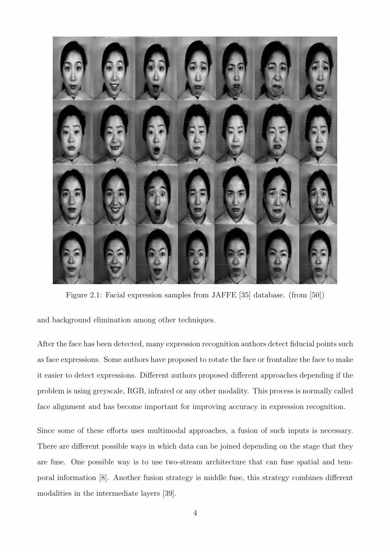
Figure 2.1: Facial expression samples from JAFFE [35] database. (from [50])

and background elimination among other techniques.

After the face has been detected, many expression recognition authors detect fiducial points such

as face expressions. Some authors have proposed to rotate the face or frontalize the face to make

it easier to detect expressions. Different authors proposed different approaches depending if the

problem is using greyscale, RGB, infrared or any other modality. This process is normally called

face alignment and has become important for improving accuracy in expression recognition.

Since some of these efforts uses multimodal approaches, a fusion of such inputs is necessary.

There are different possible ways in which data can be joined depending on the stage that they

are fuse. One possible way is to use two-stream architecture that can fuse spatial and tem-

poral information [8]. Another fusion strategy is middle fuse, this strategy combines different

modalities in the intermediate layers [39].

4

2.1.1 RGB Emotion Recognition

Originally presented by Kanade et al. [23], the Cohn-Kanade (CK) database is intended for

detecting individual facial emotion-specified expression. It was later extended into the CK+

by Lucey et al. [34]. These two datasets use 7 basic emotion categories: Anger, Contempt,

Disgust, Fear, Happy, Sadness and Surprise; and 30 facial action units (AUs) that represent

contractions of a specific set of facial muscles. Figure 2.1 shows examples of CK and CK+.

Figure 2.2: The images on the top level are from the original CK database and those on thebottom are from the CK+ database. Both dataset present 7 emotions and 30 AUs. (from [34])

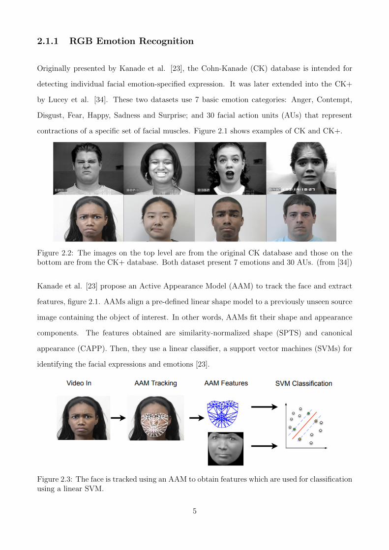
Kanade et al. [23] propose an Active Appearance Model (AAM) to track the face and extract

features, figure 2.1. AAMs align a pre-defined linear shape model to a previously unseen source

image containing the object of interest. In other words, AAMs fit their shape and appearance

components. The features obtained are similarity-normalized shape (SPTS) and canonical

appearance (CAPP). Then, they use a linear classifier, a support vector machines (SVMs) for

identifying the facial expressions and emotions [23].

Figure 2.3: The face is tracked using an AAM to obtain features which are used for classificationusing a linear SVM.

5

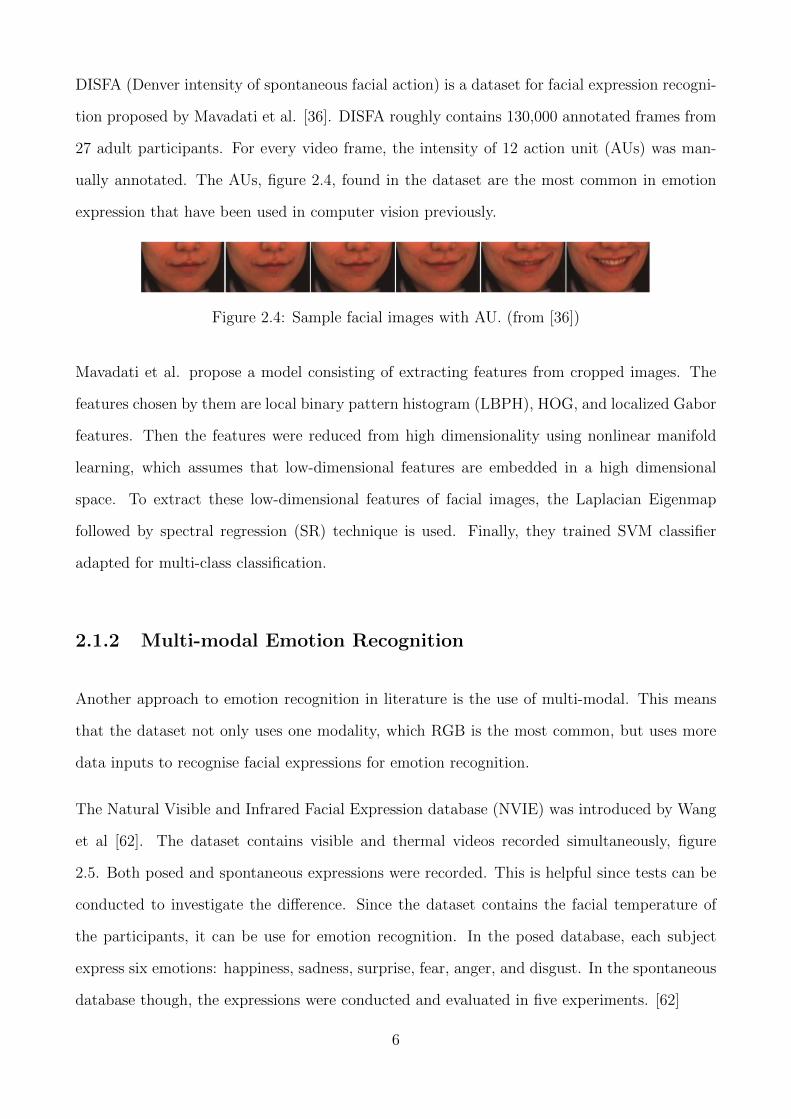
DISFA (Denver intensity of spontaneous facial action) is a dataset for facial expression recogni-

tion proposed by Mavadati et al. [36]. DISFA roughly contains 130,000 annotated frames from

27 adult participants. For every video frame, the intensity of 12 action unit (AUs) was man-

ually annotated. The AUs, figure 2.4, found in the dataset are the most common in emotion

expression that have been used in computer vision previously.

Figure 2.4: Sample facial images with AU. (from [36])

Mavadati et al. propose a model consisting of extracting features from cropped images. The

features chosen by them are local binary pattern histogram (LBPH), HOG, and localized Gabor

features. Then the features were reduced from high dimensionality using nonlinear manifold

learning, which assumes that low-dimensional features are embedded in a high dimensional

space. To extract these low-dimensional features of facial images, the Laplacian Eigenmap

followed by spectral regression (SR) technique is used. Finally, they trained SVM classifier

adapted for multi-class classification.

2.1.2 Multi-modal Emotion Recognition

Another approach to emotion recognition in literature is the use of multi-modal. This means

that the dataset not only uses one modality, which RGB is the most common, but uses more

data inputs to recognise facial expressions for emotion recognition.

The Natural Visible and Infrared Facial Expression database (NVIE) was introduced by Wang

et al [62]. The dataset contains visible and thermal videos recorded simultaneously, figure

2.5. Both posed and spontaneous expressions were recorded. This is helpful since tests can be

conducted to investigate the difference. Since the dataset contains the facial temperature of

the participants, it can be use for emotion recognition. In the posed database, each subject

express six emotions: happiness, sadness, surprise, fear, anger, and disgust. In the spontaneous

database though, the expressions were conducted and evaluated in five experiments. [62]

6

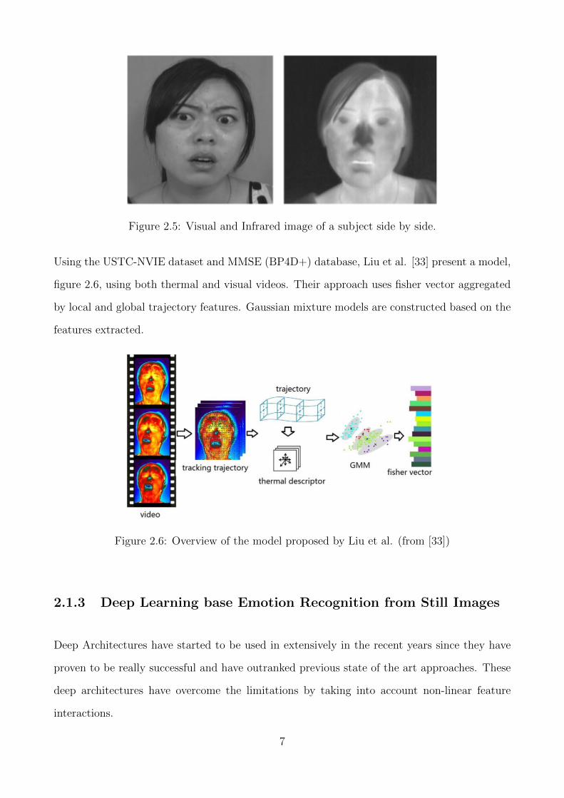
Figure 2.5: Visual and Infrared image of a subject side by side.

Using the USTC-NVIE dataset and MMSE (BP4D+) database, Liu et al. [33] present a model,

figure 2.6, using both thermal and visual videos. Their approach uses fisher vector aggregated

by local and global trajectory features. Gaussian mixture models are constructed based on the

features extracted.

Figure 2.6: Overview of the model proposed by Liu et al. (from [33])

2.1.3 Deep Learning base Emotion Recognition from Still Images

Deep Architectures have started to be used in extensively in the recent years since they have

proven to be really successful and have outranked previous state of the art approaches. These

deep architectures have overcome the limitations by taking into account non-linear feature

interactions.

7

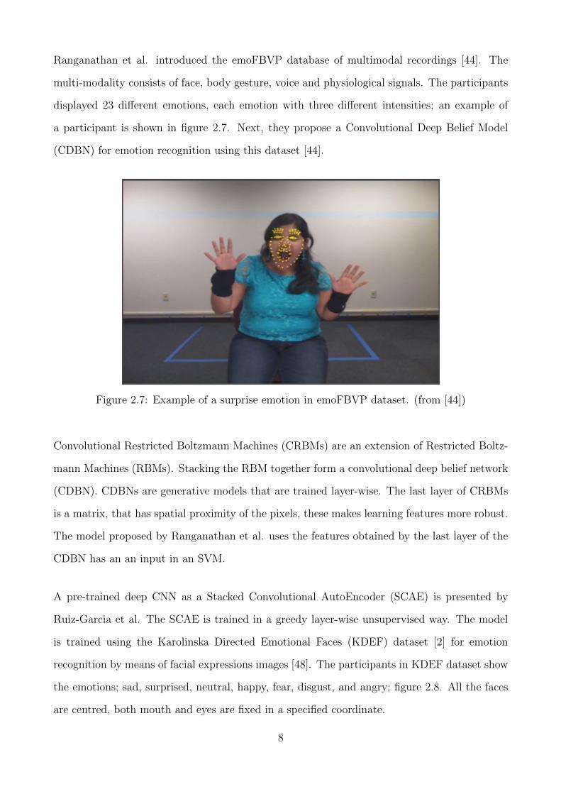
Ranganathan et al. introduced the emoFBVP database of multimodal recordings [44]. The

multi-modality consists of face, body gesture, voice and physiological signals. The participants

displayed 23 different emotions, each emotion with three different intensities; an example of

a participant is shown in figure 2.7. Next, they propose a Convolutional Deep Belief Model

(CDBN) for emotion recognition using this dataset [44].

Figure 2.7: Example of a surprise emotion in emoFBVP dataset. (from [44])

Convolutional Restricted Boltzmann Machines (CRBMs) are an extension of Restricted Boltz-

mann Machines (RBMs). Stacking the RBM together form a convolutional deep belief network

(CDBN). CDBNs are generative models that are trained layer-wise. The last layer of CRBMs

is a matrix, that has spatial proximity of the pixels, these makes learning features more robust.

The model proposed by Ranganathan et al. uses the features obtained by the last layer of the

CDBN has an an input in an SVM.

A pre-trained deep CNN as a Stacked Convolutional AutoEncoder (SCAE) is presented by

Ruiz-Garcia et al. The SCAE is trained in a greedy layer-wise unsupervised way. The model

is trained using the Karolinska Directed Emotional Faces (KDEF) dataset [2] for emotion

recognition by means of facial expressions images [48]. The participants in KDEF dataset show

the emotions; sad, surprised, neutral, happy, fear, disgust, and angry; figure 2.8. All the faces

are centred, both mouth and eyes are fixed in a specified coordinate.

8

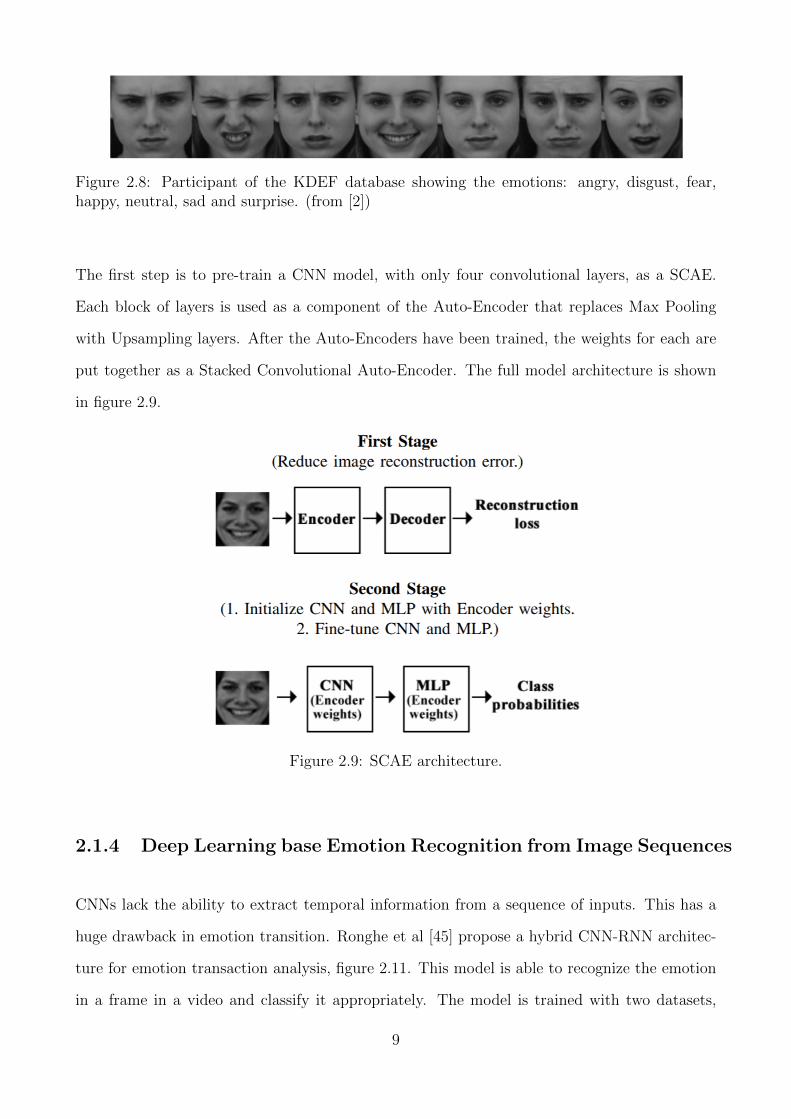
Figure 2.8: Participant of the KDEF database showing the emotions: angry, disgust, fear,happy, neutral, sad and surprise. (from [2])

The first step is to pre-train a CNN model, with only four convolutional layers, as a SCAE.

Each block of layers is used as a component of the Auto-Encoder that replaces Max Pooling

with Upsampling layers. After the Auto-Encoders have been trained, the weights for each are

put together as a Stacked Convolutional Auto-Encoder. The full model architecture is shown

in figure 2.9.

Figure 2.9: SCAE architecture.

2.1.4 Deep Learning base Emotion Recognition from Image Sequences

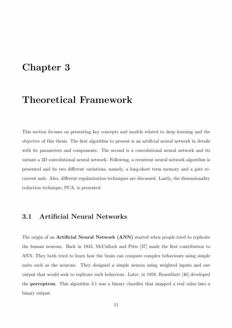
CNNs lack the ability to extract temporal information from a sequence of inputs. This has a

huge drawback in emotion transition. Ronghe et al [45] propose a hybrid CNN-RNN architec-

ture for emotion transaction analysis, figure 2.11. This model is able to recognize the emotion

in a frame in a video and classify it appropriately. The model is trained with two datasets,

9

the CASIA-Webface [66], a large-scale dataset containing about 10,000 subjects and 500,000

images, and the Emotion Recognition in the Wild [7], an audio-video based emotion and static

image based facial expression recognition.

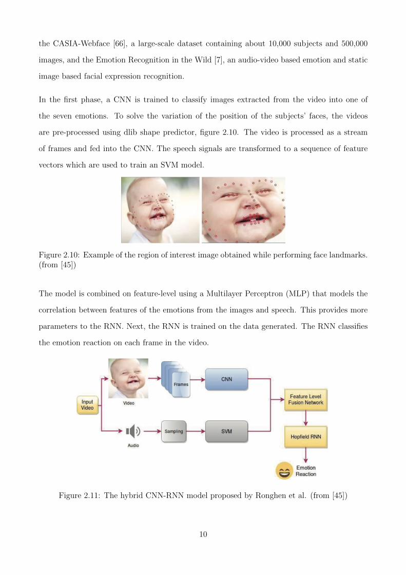
In the first phase, a CNN is trained to classify images extracted from the video into one of

the seven emotions. To solve the variation of the position of the subjects’ faces, the videos

are pre-processed using dlib shape predictor, figure 2.10. The video is processed as a stream

of frames and fed into the CNN. The speech signals are transformed to a sequence of feature

vectors which are used to train an SVM model.

Figure 2.10: Example of the region of interest image obtained while performing face landmarks.(from [45])

The model is combined on feature-level using a Multilayer Perceptron (MLP) that models the

correlation between features of the emotions from the images and speech. This provides more

parameters to the RNN. Next, the RNN is trained on the data generated. The RNN classifies

the emotion reaction on each frame in the video.

Figure 2.11: The hybrid CNN-RNN model proposed by Ronghen et al. (from [45])

10

Chapter 3

Theoretical Framework

This section focuses on presenting key concepts and models related to deep learning and the

objective of this thesis. The first algorithm to present is an artificial neural network in details

with its parameters and components. The second is a convolutional neural network and its

variant a 3D convolutional neural network. Following, a recurrent neural network algorithm is

presented and its two different variations, namely, a long-short term memory and a gate re-

current unit. Also, different regularization techniques are discussed. Lastly, the dimensionality

reduction technique, PCA, is presented.

3.1 Artificial Neural Networks

The origin of an Artificial Neural Network (ANN) started when people tried to replicate

the human neurons. Back in 1943, McCulloch and Pitts [37] made the first contribution to

ANN. They both tried to learn how the brain can compute complex behaviours using simple

units such as the neurons. They designed a simple neuron using weighted inputs and one

output that would seek to replicate such behaviour. Later, in 1958, Rosenblatt [46] developed

the perceptron. This algorithm 3.1 was a binary classifier that mapped a real value into a

binary output.

11

f(x) =

1 if w · x+ b > 0

0 otherwise(3.1)

3.1.1 Backpropagation and Stochastic Gradient Descent

In 1985, Hinton and Williams [49] rediscovered the backpropagation algorithm that was first

introduced by Werbos [63] in 1974. Backpropagation makes a forward pass of the input, when

the input reaches the last layer, the prediction is compared to the ground truth. Using a loss

function an error is calculated. The loss is then used to find the best gradient for minimizing

the error using a partial derivative. This gradient is then used to update the weights of the

last layer. Backpropagation uses the chain rule to compute the derivative of the previous layers

and update the weights of all layers.

The first proposal used Stochastic Gradient Descent (SGD). This method estimates the

best direction for optimizing the function using only a random subset of the dataset. The back-

propagation method is used iteratively until it ultimately fits the weights of all layers. Nowa-

days there exists more alternatives to SGD, these methods are called Adaptative Learning

Methods.

3.1.2 Architecture of Neural Network

A typical Neural Network (NN) has a huge number of artificial neurons, also called units,

organised in different layers [54]. An ANN can be viewed as weighted directed graph in which

artificial neurons are nodes, and directed edges with weights are connections between neuron

outputs and neuron inputs, figure 3.1.

The ANN receives information from the external world in the form of pattern and image in

vector form. These inputs are mathematically designated by the notation x(n) for n number

of inputs.

12

Each input is multiplied by its corresponding weights. Weights are the information used by the

neural network to solve a problem. Typically, weight represents the strength of the intercon-

nection between neurons inside the neural network.

Layers

The simplest form of an ANN is the Feed-Forward Neural Network (FFNN). In this kind

of network, nodes are arranged in layers. Nodes from the adjacent layers have connections

among them. These connections represent the weights between layers of nodes. Since all the

nodes of the layer are connected to all the nodes of the adjacent layer, this kind is known as

Fully Connected Layer (FC).

In a feed-forward neural network all layers are FC. Still, there can be distinguished three kinds

depending on the action they perform:

• Input layer:these layers receives data as input that will be using to learn.

• Hidden layer:these layers transform the input so that the output layer can utilise the data.

• Output layer:in this layer, the units interacts with the function that tells how it should

learn.

Neurons

The input value that neuron k in layer l receives is shown in equation 3.2. Where blk is the bias

in neuron k in layer l. Nl−1 is the number of neurons in layer l − 1. wl−1ik is the weight that

connects unit i in layer l−1 and unit k in layer l. yl−1i is the output of unit i in layer l−1. [28]

xlk = blk

Nl−1∑i=1

wl−1ik yl−1

i (3.2)

The output value that a neuron computes in a hidden layer is shown in equation 3.3. Where f

is a differentiable function of the total inputs of the neuron.

13

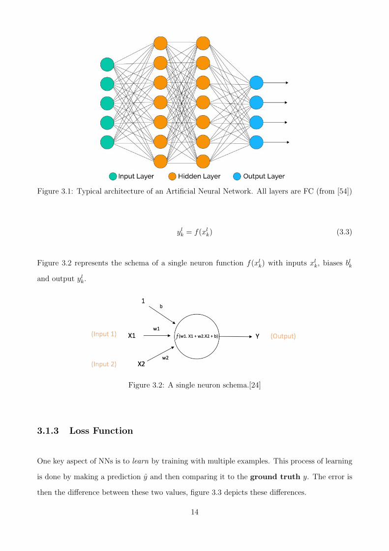
Figure 3.1: Typical architecture of an Artificial Neural Network. All layers are FC (from [54])

ylk = f(xlk) (3.3)

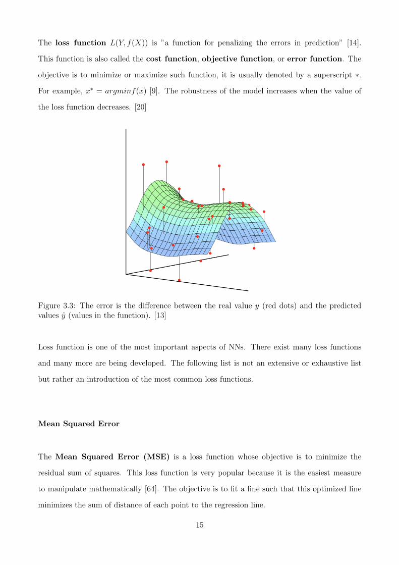
Figure 3.2 represents the schema of a single neuron function f(xlk) with inputs xlk, biases blk

and output ylk.

Figure 3.2: A single neuron schema.[24]

3.1.3 Loss Function

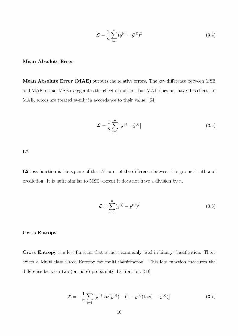
One key aspect of NNs is to learn by training with multiple examples. This process of learning

is done by making a prediction y and then comparing it to the ground truth y. The error is

then the difference between these two values, figure 3.3 depicts these differences.

14

The loss function L(Y, f(X)) is ”a function for penalizing the errors in prediction” [14].

This function is also called the cost function, objective function, or error function. The

objective is to minimize or maximize such function, it is usually denoted by a superscript ∗.

For example, x∗ = argminf(x) [9]. The robustness of the model increases when the value of

the loss function decreases. [20]

Figure 3.3: The error is the difference between the real value y (red dots) and the predictedvalues y (values in the function). [13]

Loss function is one of the most important aspects of NNs. There exist many loss functions

and many more are being developed. The following list is not an extensive or exhaustive list

but rather an introduction of the most common loss functions.

Mean Squared Error

The Mean Squared Error (MSE) is a loss function whose objective is to minimize the

residual sum of squares. This loss function is very popular because it is the easiest measure

to manipulate mathematically [64]. The objective is to fit a line such that this optimized line

minimizes the sum of distance of each point to the regression line.

15

L =1

n

n∑i=1

(y(i) − y(i))2 (3.4)

Mean Absolute Error

Mean Absolute Error (MAE) outputs the relative errors. The key difference between MSE

and MAE is that MSE exaggerates the effect of outliers, but MAE does not have this effect. In

MAE, errors are treated evenly in accordance to their value. [64]

L =1

n

n∑i=1

∣∣y(i) − y(i)∣∣ (3.5)

L2

L2 loss function is the square of the L2 norm of the difference between the ground truth and

prediction. It is quite similar to MSE, except it does not have a division by n.

L =n∑i=1

(y(i) − y(i))2 (3.6)

Cross Entropy

Cross Entropy is a loss function that is most commonly used in binary classification. There

exists a Multi-class Cross Entropy for multi-classification. This loss function measures the

difference between two (or more) probability distribution. [38]

L = − 1

n

n∑i=1

[y(i) log(y(i)) + (1− y(i)) log(1− y(i))

](3.7)

16

Hinge Loss

Hinge Loss is a loss function for training classifiers. The objective of Hinge is to maximise

the margin. This loss function is the basis of the Support Vector Machines (SVM). [38]

L =1

n

n∑i=1

max(0, 1− y(i) · y(i)) (3.8)

3.1.4 Adaptive Learning Methods

The objective of training an ANN is to perform optimization by minimizing the error using

backpropagation. Gradient Descent is one of the most popular algorithms for this task, it is

also the most common algorithm for optimizing a neural network.

The task is to follow the slope of the surface until a minimum (local minimum) is reached.

Gradient descent is an algorithms that was first used to minimize an objective function J(θ).

This objective function is parametrized by the parameters θ ∈ Rd of the model. SGD updates

the parameters in the opposite direction of the gradient from the objective function ∇θJ(θ)

w.r.t. to the parameters. This gradient is then used to traverse the surface of the objective

function. The learning rate η determines the size of the steps taken to reach this minimum.

[47]

In recent years, there has been a development of new learning methods aside from SGD. These

algorithms have tried to solve problems and challenges that SGD has. The following algorithms

are widely used in deep learning.

Momentum

Momentum is a method that helps accelerate SGD in the significant direction and get faster

convergence and also diminish the oscillations. To obtain this behaviour, momentum adds a

fraction γ of the update vector of the past time step to the current update vector as shown in

equation 3.9. [56]

17

vt = γvt−1 + η∇θJ(θ)

θ = θ − vt(3.9)

To obtain these two benefits, the momentum term γ increases when the gradients of the dimen-

sions point in the same direction and reduces updates when the gradients of the dimensions

change directions. [47]

Adagrad

Adagrad (Adaptive Gradient) is an algorithm that adapts the learning rate to the param-

eters. The algorithm makes a larger update for parameters that are not frequent and smaller

updates when the parameters are frequent. The main benefit of Adagrad is that it is no longer

needed to manually tune the learning rate. Adagrad uses different learning rate for every pa-

rameter θi at each time step t. The main weakness is that it accumulates the squared gradient

in the denominator and the sum keeps growing. This leads to the learning rate to shrink and

become extremely small where it can no longer acquire knowledge from the gradient. [17]

The gradient of the objective function, equation 3.10 [17], is defined as gt,i w.r.t. to the

parameter θi at time step t.

gt,i = ∆θJ(θt,i) (3.10)

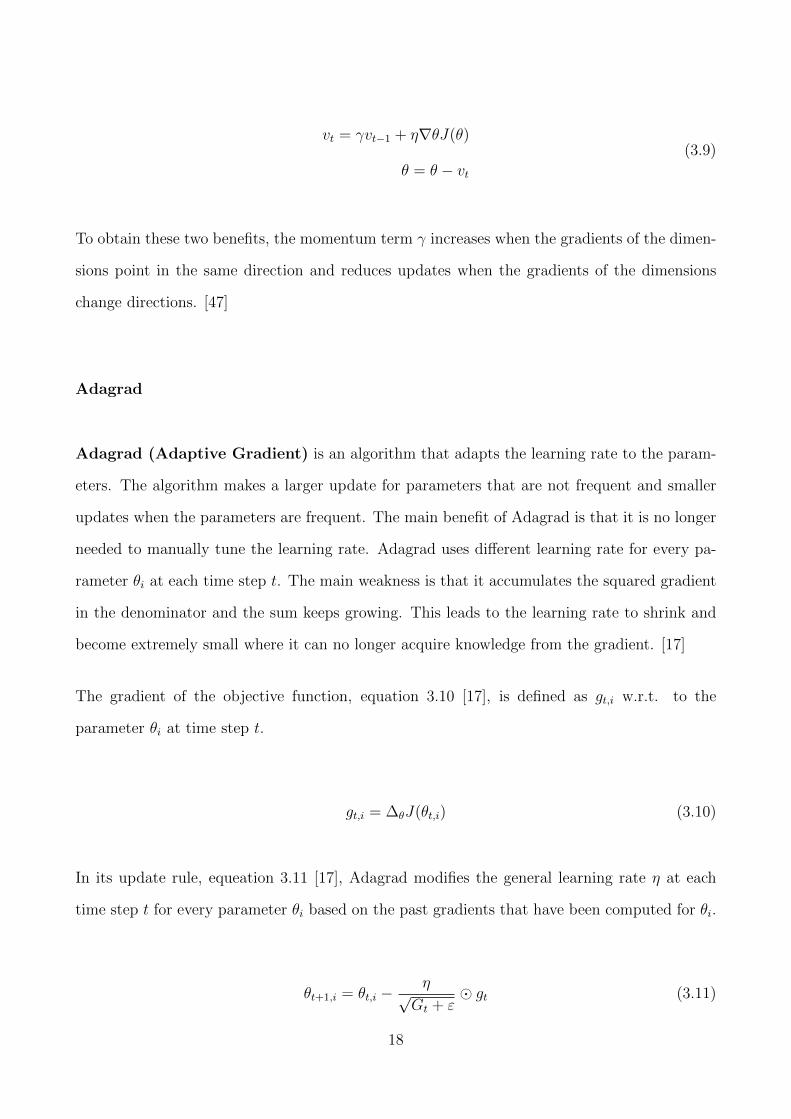
In its update rule, equeation 3.11 [17], Adagrad modifies the general learning rate η at each

time step t for every parameter θi based on the past gradients that have been computed for θi.

θt+1,i = θt,i −η√

Gt + ε� gt (3.11)

18

Adadelta

Adadelta tries to solve the problem of the shrinking rate of Adagrad. To solve it, Adadelta

restricts the accumulation of past gradient with a windows size w. [67]

Adadelta stores the sum of gradients but it recursively defines it as a decaying average of the

previous squared gradients. This average E[g2]t, at time step t, depends on the previous average

and the current gradient.

Using equation 3.11 from Adagrad. The new update equation from Adadelta replaces Gt with

the average of the precious squared gradient. The update equation is as follow:

θt+1,i = θt,i −η√

E[g2]t + ε� gt (3.12)

Since the update needs to have the same hypothetical units. The learning rate is replaced with

another exponentially decaying average. In this case, instead of the updates of the squared

gradients, the squared parameter updates are used instead E[∆θ2]t. Since this parameter at

time step t is unknown, the parameter at time step t − 1 is used instead E[∆θ2]t−1 and then

the root mean squared of this parameter.

Since both the numerator and the denominator are root mean squared, the short-hand is used

(RMS). The final update equation for Adadelta is:

θt+1,i = −RMS[∆θ]t−1

RMS[g]tgt

θt+1 = θt + ∆θt+1

(3.13)

RMSprop

RMSprop is a method introduced by Hinton [15], that also tries to solve the issue with the

shrinking learning rate of Adagrad. Similar to what Adadelta does, RMSprop divides the

19

learning rate by an exponentially decaying average of squared gradients. [47] RMSprop is

actually equal to the first update of Adadelta:

E[g2]t = 0.9E[g2]t−1 + 0.1g2t

θt+1,i = θt,i −η√

E[g2]t + εgt

(3.14)

Adam

Adam (Adaptive Moment Estimation) [27] calculates adaptive learning rates, that are

calculated for all parameters. Like Adadelta and RMSprop, Adam also calculates the exponen-

tially decaying average of past squared gradients. Adam, however, also keeps an exponentially

decaying average of past gradients mt like Momentum; and also, an estimate of the second

moment vt. [47]

mt = β1mt−1 + (1− β1)gt

vt = β2vt−1 + (1− β2)g2t(3.15)

There are biased towards zero when the decay rates are small. To avoid this, some bias correc-

tions are computed:

mt =mt

1− βt2

mt =vt

1− βt2

(3.16)

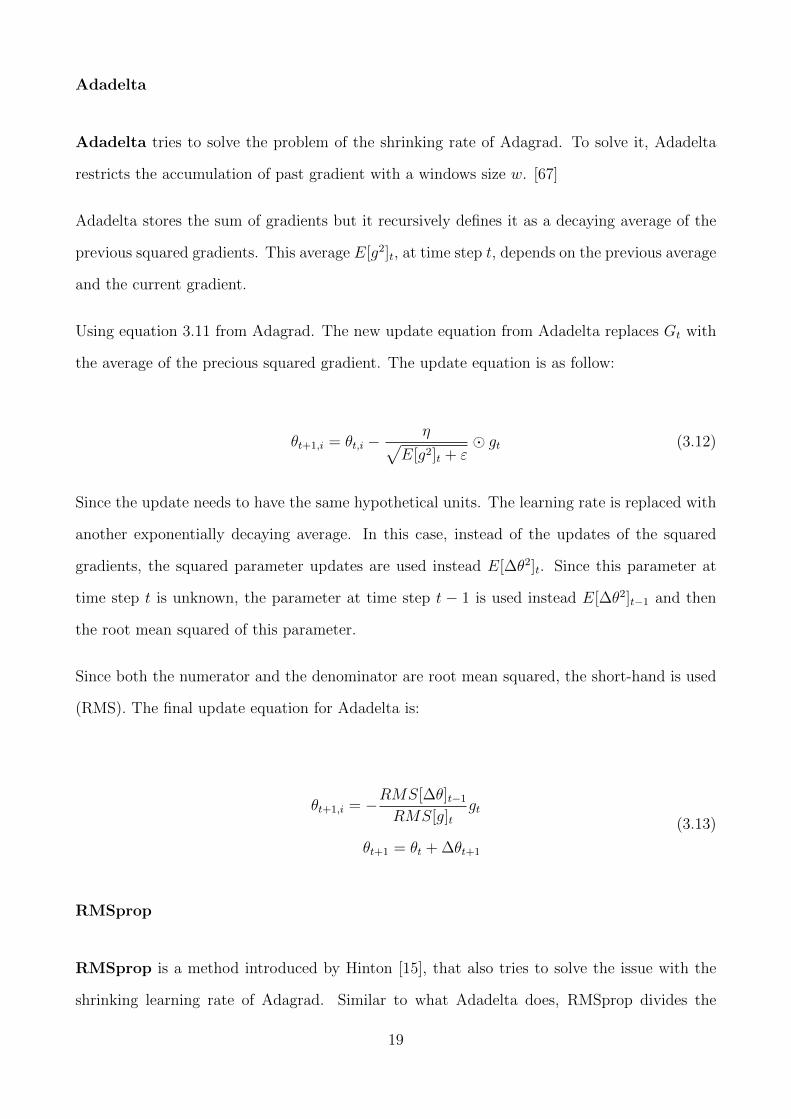
The update formula is:

θt+1 = θt −η√vt + ε

mt (3.17)

20

3.1.5 Activation Functions

In an artificial neural network, not all neurons always activate. There exists a threshold for a

neuron to be activated. The neuron calculates the input with an activation function and then

it sends the result as an output. The activation function is then used to decide when the

connection fires or not a neuron. Activation functions can be any function, although in deep

architectures the activation functions are used for non-linear operations.

3.1.6 Sigmoid

Sigmoid function is one of the most widely used in neural network. The non-linear nature of

the sigmoid function makes that any combination also non-linear and ideal for neural networks.

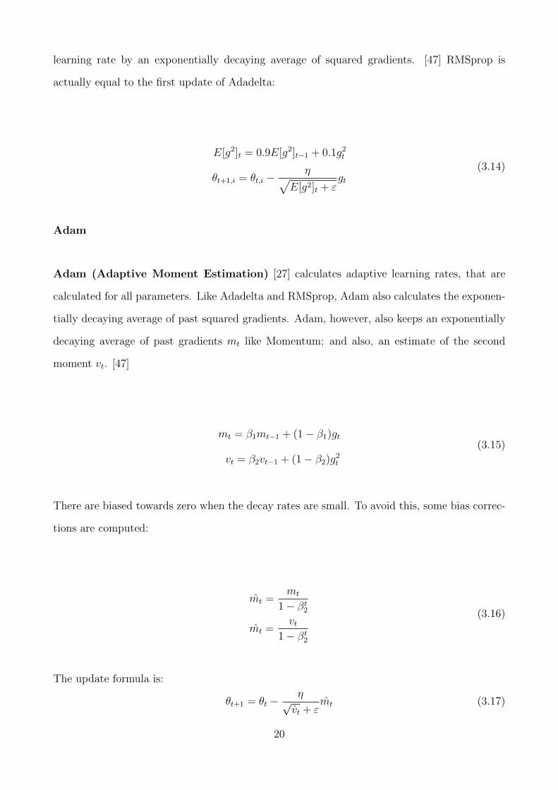
f(x) =1

1 + e−x(3.18)

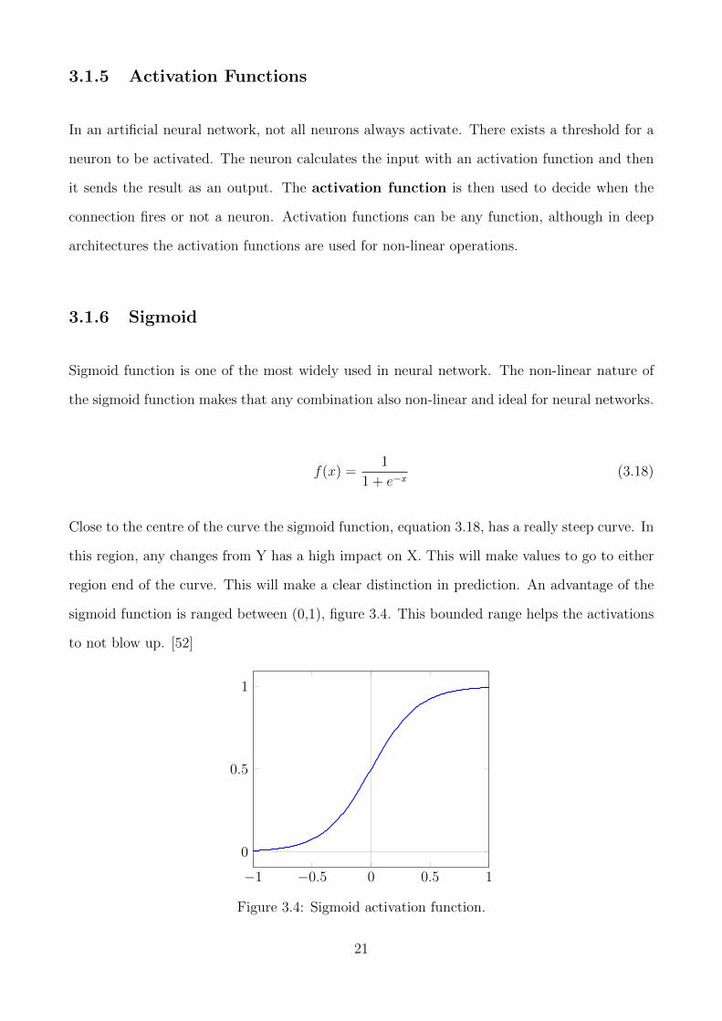
Close to the centre of the curve the sigmoid function, equation 3.18, has a really steep curve. In

this region, any changes from Y has a high impact on X. This will make values to go to either

region end of the curve. This will make a clear distinction in prediction. An advantage of the

sigmoid function is ranged between (0,1), figure 3.4. This bounded range helps the activations

to not blow up. [52]

−1 −0.5 0 0.5 1

0

0.5

1

Figure 3.4: Sigmoid activation function.

21

However, close to the end of either sigmoid function, the values of Y respond less to the values

of X. In this part, the gradient at that region is really small. This results in a problem known as

’vanishing gradient’. In this part of the curve, the gradient is so small that the neural network

cannot learn further. By multiplying such small gradients the values will tend more to zero

and thus making the learning process infeasible.

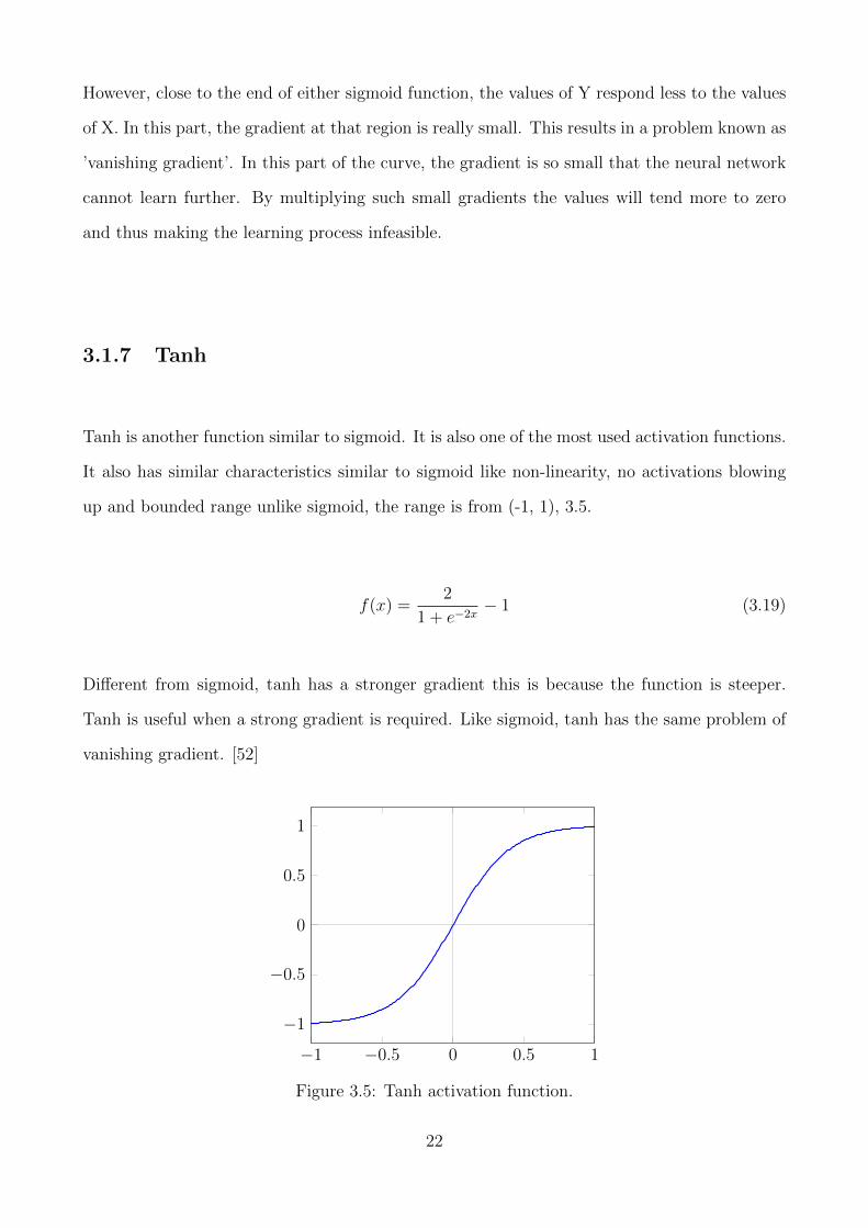
3.1.7 Tanh

Tanh is another function similar to sigmoid. It is also one of the most used activation functions.

It also has similar characteristics similar to sigmoid like non-linearity, no activations blowing

up and bounded range unlike sigmoid, the range is from (-1, 1), 3.5.

f(x) =2

1 + e−2x− 1 (3.19)

Different from sigmoid, tanh has a stronger gradient this is because the function is steeper.

Tanh is useful when a strong gradient is required. Like sigmoid, tanh has the same problem of

vanishing gradient. [52]

−1 −0.5 0 0.5 1

−1

−0.5

0

0.5

1

Figure 3.5: Tanh activation function.

22

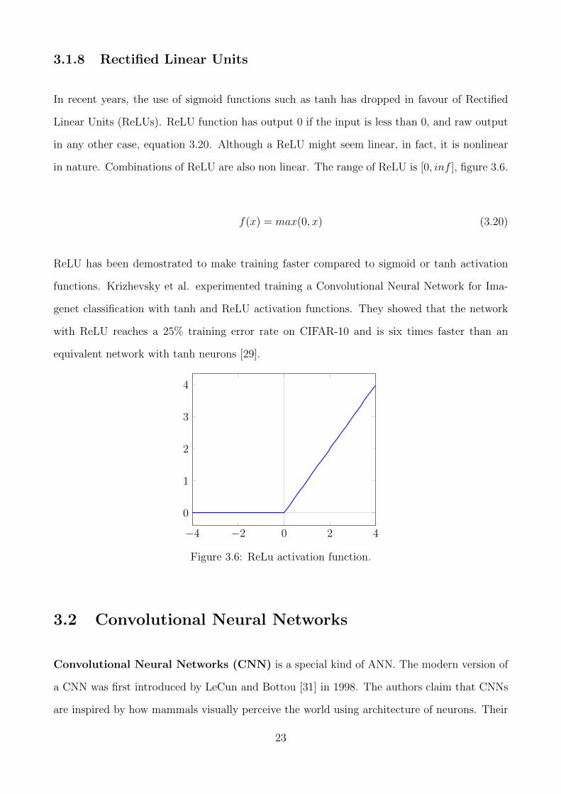
3.1.8 Rectified Linear Units

In recent years, the use of sigmoid functions such as tanh has dropped in favour of Rectified

Linear Units (ReLUs). ReLU function has output 0 if the input is less than 0, and raw output

in any other case, equation 3.20. Although a ReLU might seem linear, in fact, it is nonlinear

in nature. Combinations of ReLU are also non linear. The range of ReLU is [0, inf ], figure 3.6.

f(x) = max(0, x) (3.20)

ReLU has been demostrated to make training faster compared to sigmoid or tanh activation

functions. Krizhevsky et al. experimented training a Convolutional Neural Network for Ima-

genet classification with tanh and ReLU activation functions. They showed that the network

with ReLU reaches a 25% training error rate on CIFAR-10 and is six times faster than an

equivalent network with tanh neurons [29].

−4 −2 0 2 4

0

1

2

3

4

Figure 3.6: ReLu activation function.

3.2 Convolutional Neural Networks

Convolutional Neural Networks (CNN) is a special kind of ANN. The modern version of

a CNN was first introduced by LeCun and Bottou [31] in 1998. The authors claim that CNNs

are inspired by how mammals visually perceive the world using architecture of neurons. Their

23

work was inspired by a research investigation by Hubel and Wiesel [19] in which they describe

in detail the mammal’s visual perception architecture.

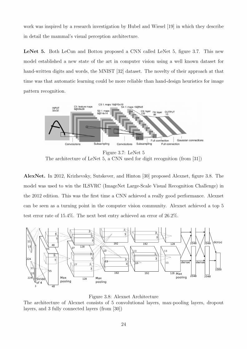
LeNet 5. Both LeCun and Bottou proposed a CNN called LeNet 5, figure 3.7. This new

model established a new state of the art in computer vision using a well known dataset for

hand-written digits and words, the MNIST [32] dataset. The novelty of their approach at that

time was that automatic learning could be more reliable than hand-design heuristics for image

pattern recognition.

Figure 3.7: LeNet 5The architecture of LeNet 5, a CNN used for digit recognition (from [31])

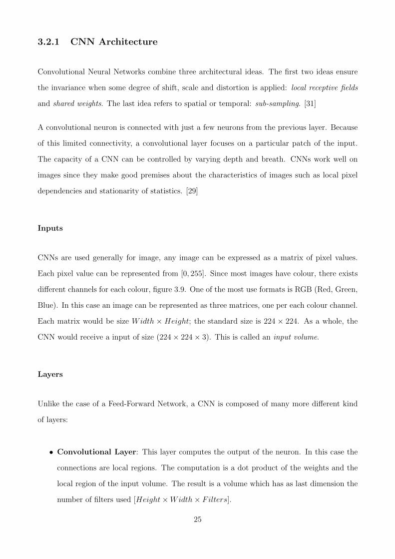
AlexNet. In 2012, Krizhevsky, Sutskever, and Hinton [30] proposed Alexnet, figure 3.8. The

model was used to win the ILSVRC (ImageNet Large-Scale Visual Recognition Challenge) in

the 2012 edition. This was the first time a CNN achieved a really good performance. Alexnet

can be seen as a turning point in the computer vision community. Alexnet achieved a top 5

test error rate of 15.4%. The next best entry achieved an error of 26.2%.

Figure 3.8: Alexnet ArchitectureThe architecture of Alexnet consists of 5 convolutional layers, max-pooling layers, dropoutlayers, and 3 fully connected layers (from [30])

24

3.2.1 CNN Architecture

Convolutional Neural Networks combine three architectural ideas. The first two ideas ensure

the invariance when some degree of shift, scale and distortion is applied: local receptive fields

and shared weights. The last idea refers to spatial or temporal: sub-sampling. [31]

A convolutional neuron is connected with just a few neurons from the previous layer. Because

of this limited connectivity, a convolutional layer focuses on a particular patch of the input.

The capacity of a CNN can be controlled by varying depth and breath. CNNs work well on

images since they make good premises about the characteristics of images such as local pixel

dependencies and stationarity of statistics. [29]

Inputs

CNNs are used generally for image, any image can be expressed as a matrix of pixel values.

Each pixel value can be represented from [0, 255]. Since most images have colour, there exists

different channels for each colour, figure 3.9. One of the most use formats is RGB (Red, Green,

Blue). In this case an image can be represented as three matrices, one per each colour channel.

Each matrix would be size Width × Height; the standard size is 224 × 224. As a whole, the

CNN would receive a input of size (224× 224× 3). This is called an input volume.

Layers

Unlike the case of a Feed-Forward Network, a CNN is composed of many more different kind

of layers:

• Convolutional Layer: This layer computes the output of the neuron. In this case the

connections are local regions. The computation is a dot product of the weights and the

local region of the input volume. The result is a volume which has as last dimension the

number of filters used [Height×Width× Filters].

25

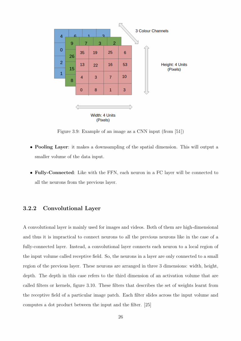
Figure 3.9: Example of an image as a CNN input (from [51])

• Pooling Layer: it makes a downsampling of the spatial dimension. This will output a

smaller volume of the data input.

• Fully-Connected: Like with the FFN, each neuron in a FC layer will be connected to

all the neurons from the previous layer.

3.2.2 Convolutional Layer

A convolutional layer is mainly used for images and videos. Both of them are high-dimensional

and thus it is impractical to connect neurons to all the previous neurons like in the case of a

fully-connected layer. Instead, a convolutional layer connects each neuron to a local region of

the input volume called receptive field. So, the neurons in a layer are only connected to a small

region of the previous layer. These neurons are arranged in three 3 dimensions: width, height,

depth. The depth in this case refers to the third dimension of an activation volume that are

called filters or kernels, figure 3.10. These filters that describes the set of weights learnt from

the receptive field of a particular image patch. Each filter slides across the input volume and

computes a dot product between the input and the filter. [25]

26

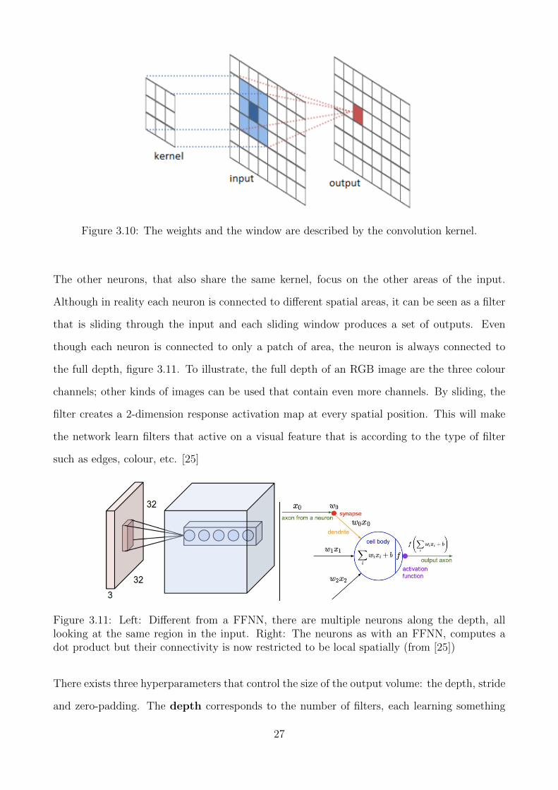
Figure 3.10: The weights and the window are described by the convolution kernel.

The other neurons, that also share the same kernel, focus on the other areas of the input.

Although in reality each neuron is connected to different spatial areas, it can be seen as a filter

that is sliding through the input and each sliding window produces a set of outputs. Even

though each neuron is connected to only a patch of area, the neuron is always connected to

the full depth, figure 3.11. To illustrate, the full depth of an RGB image are the three colour

channels; other kinds of images can be used that contain even more channels. By sliding, the

filter creates a 2-dimension response activation map at every spatial position. This will make

the network learn filters that active on a visual feature that is according to the type of filter

such as edges, colour, etc. [25]

Figure 3.11: Left: Different from a FFNN, there are multiple neurons along the depth, alllooking at the same region in the input. Right: The neurons as with an FFNN, computes adot product but their connectivity is now restricted to be local spatially (from [25])

There exists three hyperparameters that control the size of the output volume: the depth, stride

and zero-padding. The depth corresponds to the number of filters, each learning something

27

different from the input. As an example, some might look for different oriented edges, or blobs

of colour. The stride is how many pixels the filter is slide. When the slide corresponds to 1

then the filter is moved one pixel at a time. If the stride is 2 then there will be a jump of 2

pixels. The zero-padding correspond to adding zeros to the border of the input. This will

allow to control the spatial size of the output volume. [25]

3.2.3 Fully-Connected Layer

Like with a Feed-Forward Neural Network, a fully-connected layer has full connections to all

activations in the previous layer. [25]

3.2.4 Pooling Layer

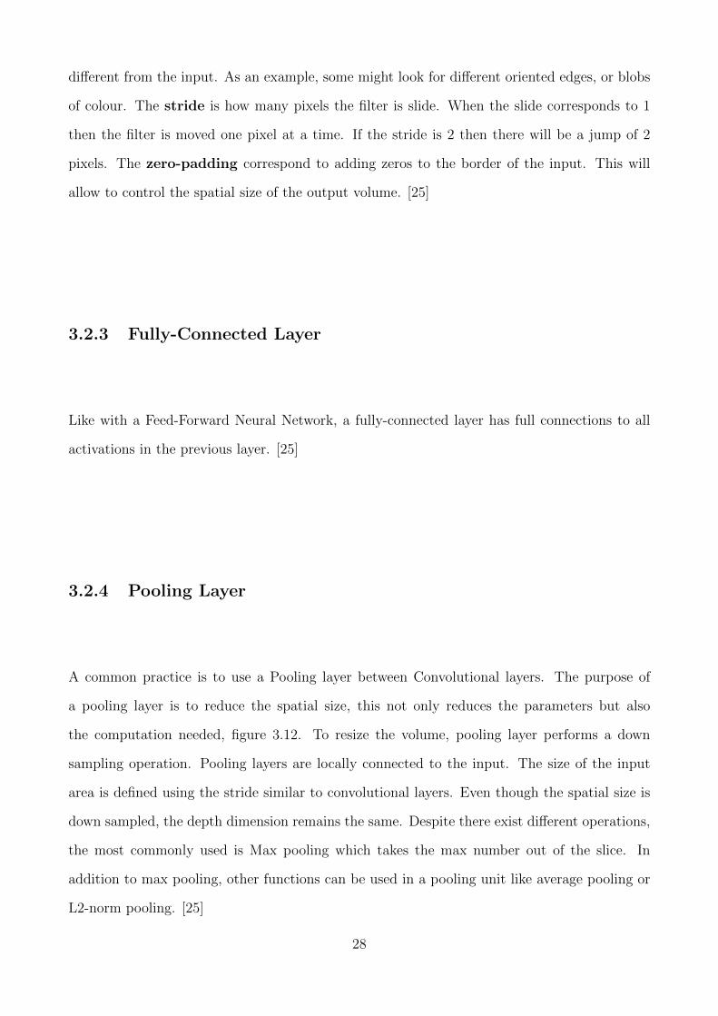
A common practice is to use a Pooling layer between Convolutional layers. The purpose of

a pooling layer is to reduce the spatial size, this not only reduces the parameters but also

the computation needed, figure 3.12. To resize the volume, pooling layer performs a down

sampling operation. Pooling layers are locally connected to the input. The size of the input

area is defined using the stride similar to convolutional layers. Even though the spatial size is

down sampled, the depth dimension remains the same. Despite there exist different operations,

the most commonly used is Max pooling which takes the max number out of the slice. In

addition to max pooling, other functions can be used in a pooling unit like average pooling or

L2-norm pooling. [25]

28

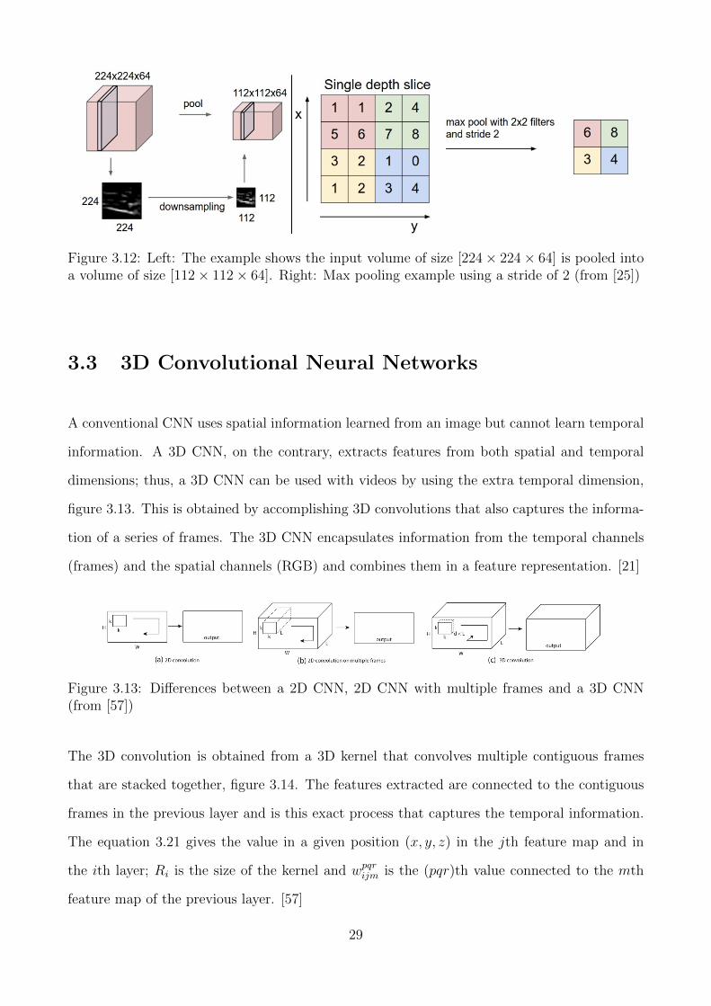
Figure 3.12: Left: The example shows the input volume of size [224× 224× 64] is pooled intoa volume of size [112× 112× 64]. Right: Max pooling example using a stride of 2 (from [25])

3.3 3D Convolutional Neural Networks

A conventional CNN uses spatial information learned from an image but cannot learn temporal

information. A 3D CNN, on the contrary, extracts features from both spatial and temporal

dimensions; thus, a 3D CNN can be used with videos by using the extra temporal dimension,

figure 3.13. This is obtained by accomplishing 3D convolutions that also captures the informa-

tion of a series of frames. The 3D CNN encapsulates information from the temporal channels

(frames) and the spatial channels (RGB) and combines them in a feature representation. [21]

Figure 3.13: Differences between a 2D CNN, 2D CNN with multiple frames and a 3D CNN(from [57])

The 3D convolution is obtained from a 3D kernel that convolves multiple contiguous frames

that are stacked together, figure 3.14. The features extracted are connected to the contiguous

frames in the previous layer and is this exact process that captures the temporal information.

The equation 3.21 gives the value in a given position (x, y, z) in the jth feature map and in

the ith layer; Ri is the size of the kernel and wpqrijm is the (pqr)th value connected to the mth

feature map of the previous layer. [57]

29

vxyzij = tanh

(bij +

∑m

Pi−1∑p=0

Qi−1∑q=0

Ri−1∑r=0

wpqrijmv(x+p)(y+q)(z+r)(i−1)m

)(3.21)

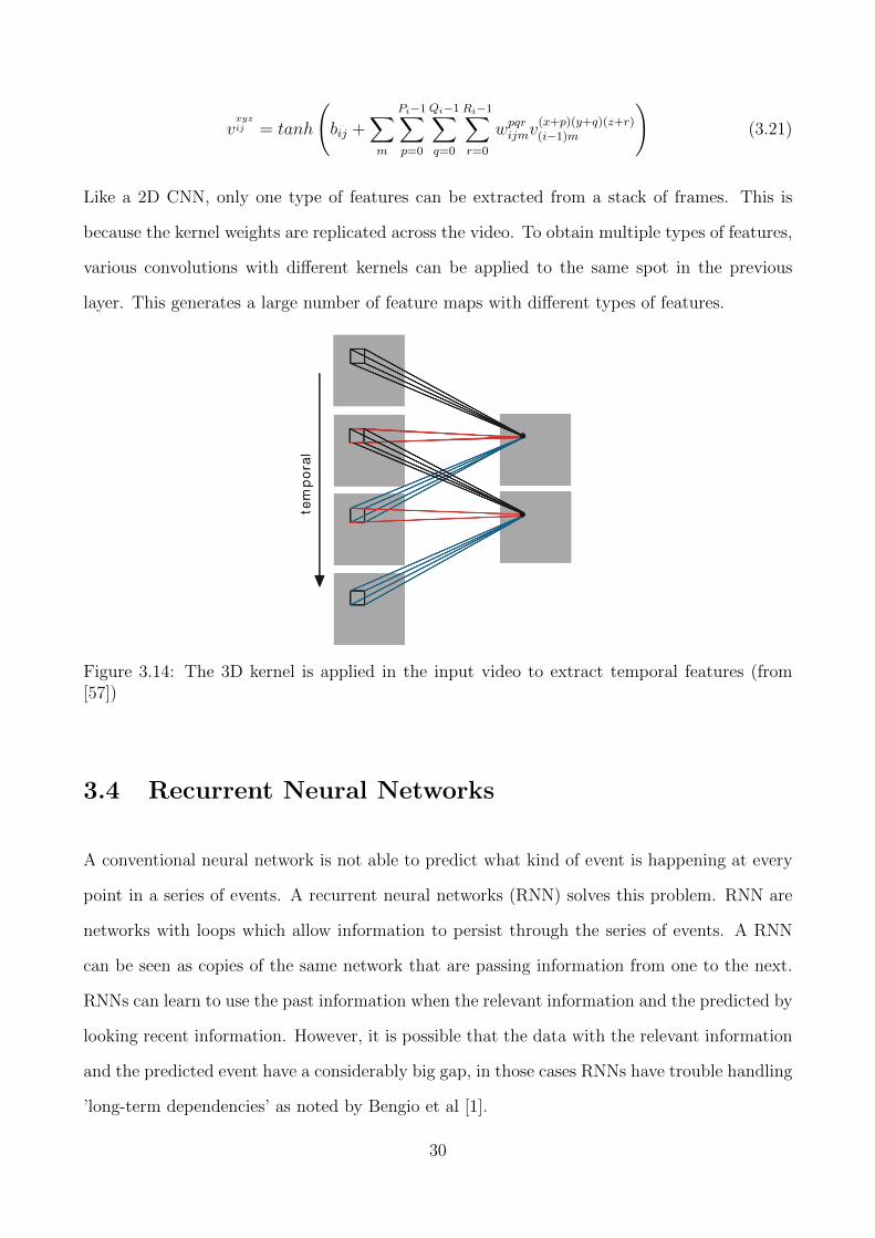
Like a 2D CNN, only one type of features can be extracted from a stack of frames. This is

because the kernel weights are replicated across the video. To obtain multiple types of features,

various convolutions with different kernels can be applied to the same spot in the previous

layer. This generates a large number of feature maps with different types of features.

Figure 3.14: The 3D kernel is applied in the input video to extract temporal features (from[57])

3.4 Recurrent Neural Networks

A conventional neural network is not able to predict what kind of event is happening at every

point in a series of events. A recurrent neural networks (RNN) solves this problem. RNN are

networks with loops which allow information to persist through the series of events. A RNN

can be seen as copies of the same network that are passing information from one to the next.

RNNs can learn to use the past information when the relevant information and the predicted by

looking recent information. However, it is possible that the data with the relevant information

and the predicted event have a considerably big gap, in those cases RNNs have trouble handling

’long-term dependencies’ as noted by Bengio et al [1].

30

3.5 Long Short-Term Memory

Long Short Term Memory networks (LSTM), first introduced by Hochreiter and Schmid-

huber [16], solved the problem of long-term dependencies. These special kind of RNNs are

capable of learning both short-term and long-term dependencies although they are specialised

for long-term relationships.

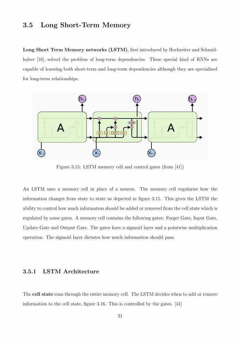
Figure 3.15: LSTM memory cell and control gates (from [41])

An LSTM uses a memory cell in place of a neuron. The memory cell regularise how the

information changes from state to state as depicted in figure 3.15. This gives the LSTM the

ability to control how much information should be added or removed from the cell state which is

regulated by some gates. A memory cell contains the following gates: Forget Gate, Input Gate,

Update Gate and Output Gate. The gates have a sigmoid layer and a pointwise multiplication

operation. The sigmoid layer dictates how much information should pass.

3.5.1 LSTM Architecture

The cell state runs through the entire memory cell. The LSTM decides when to add or remove

information to the cell state, figure 3.16. This is controlled by the gates. [41]

31

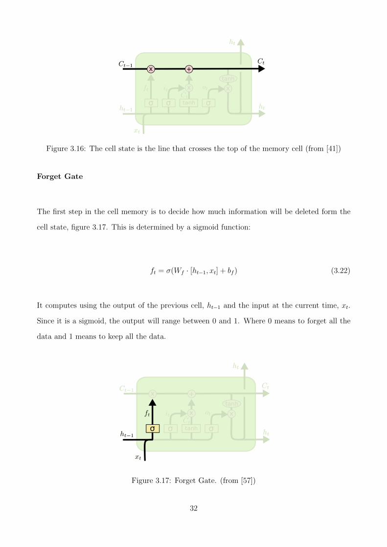
Figure 3.16: The cell state is the line that crosses the top of the memory cell (from [41])

Forget Gate

The first step in the cell memory is to decide how much information will be deleted form the

cell state, figure 3.17. This is determined by a sigmoid function:

ft = σ(Wf · [ht−1, xt] + bf ) (3.22)

It computes using the output of the previous cell, ht−1 and the input at the current time, xt.

Since it is a sigmoid, the output will range between 0 and 1. Where 0 means to forget all the

data and 1 means to keep all the data.

Figure 3.17: Forget Gate. (from [57])

32

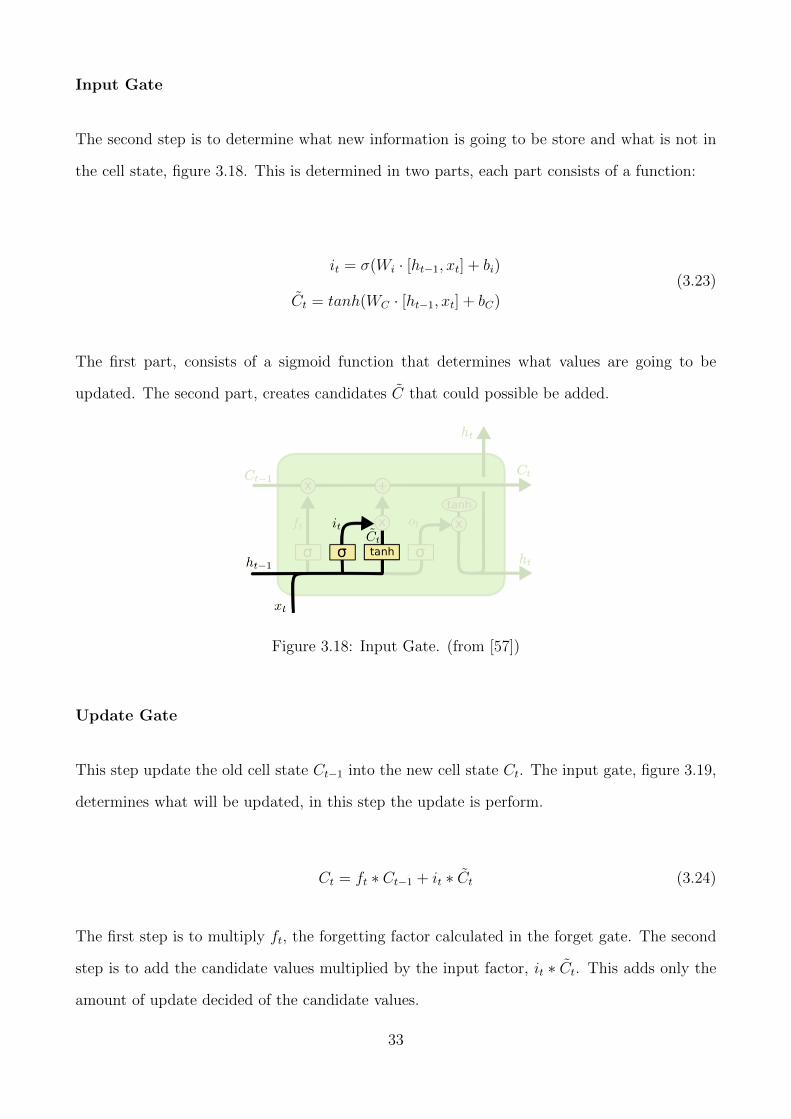
Input Gate

The second step is to determine what new information is going to be store and what is not in

the cell state, figure 3.18. This is determined in two parts, each part consists of a function:

it = σ(Wi · [ht−1, xt] + bi)

Ct = tanh(WC · [ht−1, xt] + bC)

(3.23)

The first part, consists of a sigmoid function that determines what values are going to be

updated. The second part, creates candidates C that could possible be added.

Figure 3.18: Input Gate. (from [57])

Update Gate

This step update the old cell state Ct−1 into the new cell state Ct. The input gate, figure 3.19,

determines what will be updated, in this step the update is perform.

Ct = ft ∗ Ct−1 + it ∗ Ct (3.24)

The first step is to multiply ft, the forgetting factor calculated in the forget gate. The second

step is to add the candidate values multiplied by the input factor, it ∗ Ct. This adds only the

amount of update decided of the candidate values.

33

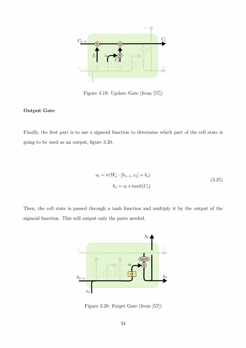
Figure 3.19: Update Gate (from [57])

Output Gate

Finally, the first part is to use a sigmoid function to determine which part of the cell state is

going to be used as an output, figure 3.20.

ot = σ(Wo · [ht−1, xt] + bo)

ht = ot ∗ tanh(Ct)

(3.25)

Then, the cell state is passed through a tanh function and multiply it by the output of the

sigmoid function. This will output only the parts needed.

Figure 3.20: Forget Gate (from [57])

34

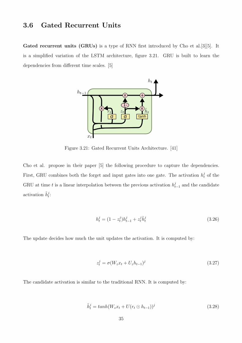
3.6 Gated Recurrent Units

Gated recurrent units (GRUs) is a type of RNN first introduced by Cho et al.[3][5]. It

is a simplified variation of the LSTM architecture, figure 3.21. GRU is built to learn the

dependencies from different time scales. [5]

Figure 3.21: Gated Recurrent Units Architecture. [41]

Cho et al. propose in their paper [5] the following procedure to capture the dependencies.

First, GRU combines both the forget and input gates into one gate. The activation hjt of the

GRU at time t is a linear interpolation between the previous activation hjt−1 and the candidate

activation hjt :

hjt = (1− zjt )hjt−1 + zjt h

jt (3.26)

The update decides how much the unit updates the activation. It is computed by:

zjt = σ(Wzxt + Uzht−1)j (3.27)

The candidate activation is similar to the traditional RNN. It is computed by:

hjt = tanh(Wzxt + U(rt � ht−1))j (3.28)

35

the reset gate makes the unit forget previous computed states. It is computed by:

rjt = σ(Wrxt + Urht−1)j (3.29)

3.7 Reducing Overfitting

Deep architectures usually have millions of parameters, each layer is connected by weight con-

nections. Many of these relationships can become really complicated, which are the result of

sampling noise. These models with a lot of parameters can easily overfit the training data.

Much of the noise exists in the training set but not in test or real data even if they are drawn

from the same distribution. To help avoid this problem, there exist methods that have been

developed to help reduce it.

3.7.1 L1/L2 Regularization

L1 and L2 regularization adds a penalty term that prevents the coefficient to fit perfectly to the

data, thus preventing overfitting. This causes the model to fit less to the noise of the training

data which in turn improves the model generalization.

The L1 regularization term, shown in equation 3.30, is the absolute sum of the weights

multiplied by the coefficient. [38]

w∗ = argminw

∑j

(t(xj)−

∑i

wihi(xj)

)2

+ λk∑i=1

|wi| (3.30)

The L2 regularization term in equation 3.31, is the sum of the square of the weights multiplied

by the coefficient. [38]

w∗ = argminw

∑j

(t(xj)−

∑i

wihi(xj)

)2

+ λk∑i=1

w2i (3.31)

36

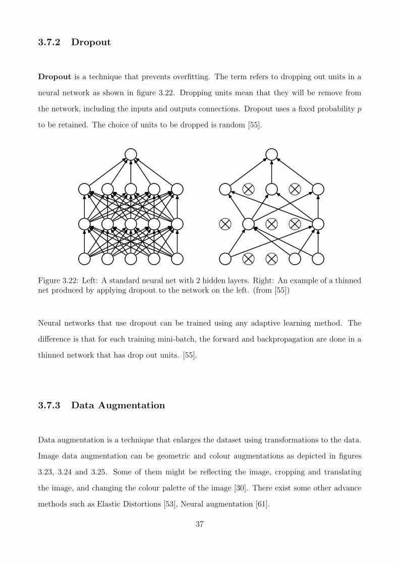
3.7.2 Dropout

Dropout is a technique that prevents overfitting. The term refers to dropping out units in a

neural network as shown in figure 3.22. Dropping units mean that they will be remove from

the network, including the inputs and outputs connections. Dropout uses a fixed probability p

to be retained. The choice of units to be dropped is random [55].

Figure 3.22: Left: A standard neural net with 2 hidden layers. Right: An example of a thinnednet produced by applying dropout to the network on the left. (from [55])

Neural networks that use dropout can be trained using any adaptive learning method. The

difference is that for each training mini-batch, the forward and backpropagation are done in a

thinned network that has drop out units. [55].

3.7.3 Data Augmentation

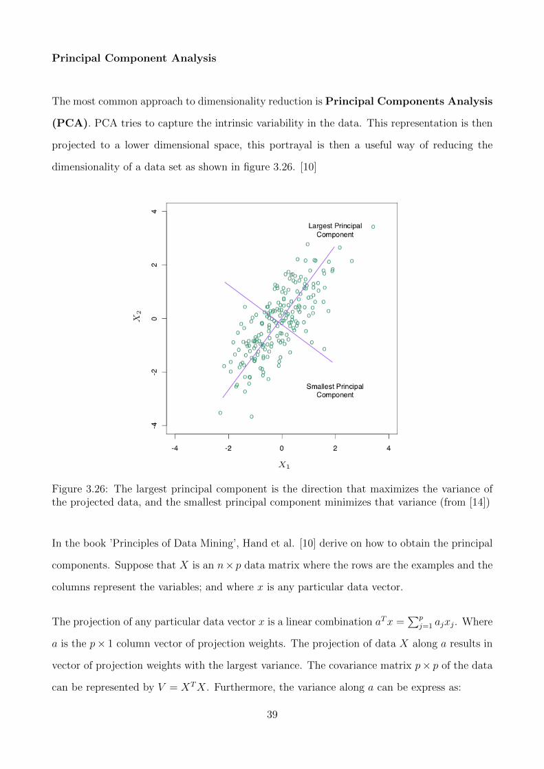
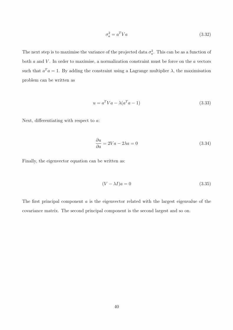
Data augmentation is a technique that enlarges the dataset using transformations to the data.

Image data augmentation can be geometric and colour augmentations as depicted in figures

3.23, 3.24 and 3.25. Some of them might be reflecting the image, cropping and translating

the image, and changing the colour palette of the image [30]. There exist some other advance

methods such as Elastic Distortions [53], Neural augmentation [61].

37

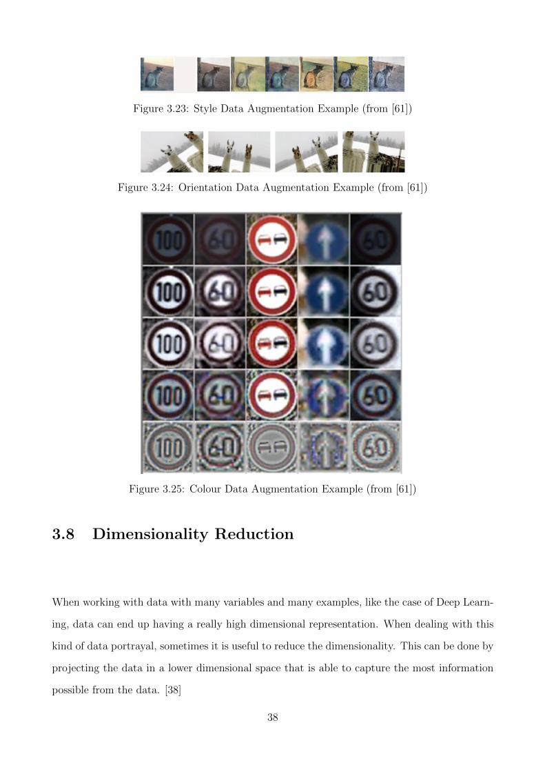
Figure 3.23: Style Data Augmentation Example (from [61])

Figure 3.24: Orientation Data Augmentation Example (from [61])

Figure 3.25: Colour Data Augmentation Example (from [61])

3.8 Dimensionality Reduction

When working with data with many variables and many examples, like the case of Deep Learn-

ing, data can end up having a really high dimensional representation. When dealing with this

kind of data portrayal, sometimes it is useful to reduce the dimensionality. This can be done by

projecting the data in a lower dimensional space that is able to capture the most information

possible from the data. [38]

38

Principal Component Analysis

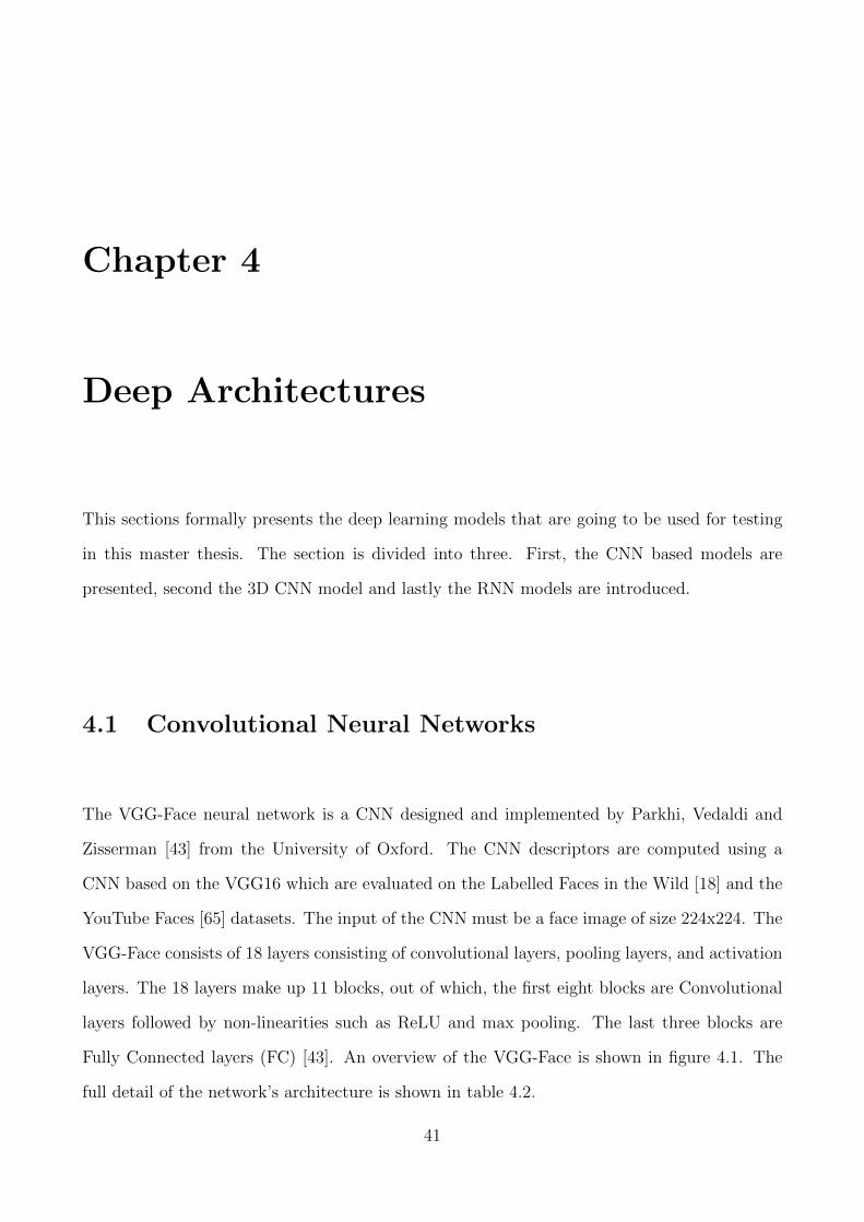
The most common approach to dimensionality reduction is Principal Components Analysis

(PCA). PCA tries to capture the intrinsic variability in the data. This representation is then

projected to a lower dimensional space, this portrayal is then a useful way of reducing the

dimensionality of a data set as shown in figure 3.26. [10]

Figure 3.26: The largest principal component is the direction that maximizes the variance ofthe projected data, and the smallest principal component minimizes that variance (from [14])

In the book ’Principles of Data Mining’, Hand et al. [10] derive on how to obtain the principal

components. Suppose that X is an n× p data matrix where the rows are the examples and the

columns represent the variables; and where x is any particular data vector.

The projection of any particular data vector x is a linear combination aTx =∑p

j=1 ajxj. Where

a is the p× 1 column vector of projection weights. The projection of data X along a results in

vector of projection weights with the largest variance. The covariance matrix p× p of the data

can be represented by V = XTX. Furthermore, the variance along a can be express as:

39

σ2a = aTV a (3.32)

The next step is to maximise the variance of the projected data σ2a. This can be as a function of

both a and V . In order to maximise, a normalization constraint must be force on the a vectors

such that aTa = 1. By adding the constraint using a Lagrange multiplier λ, the maximisation

problem can be written as

u = aTV a− λ(aTa− 1) (3.33)

Next, differentiating with respect to a:

∂u

∂a= 2V a− 2λa = 0 (3.34)

Finally, the eigenvector equation can be written as:

(V − λI)a = 0 (3.35)

The first principal component a is the eigenvector related with the largest eigenvalue of the

covariance matrix. The second principal component is the second largest and so on.

40

Chapter 4

Deep Architectures

This sections formally presents the deep learning models that are going to be used for testing

in this master thesis. The section is divided into three. First, the CNN based models are

presented, second the 3D CNN model and lastly the RNN models are introduced.

4.1 Convolutional Neural Networks

The VGG-Face neural network is a CNN designed and implemented by Parkhi, Vedaldi and

Zisserman [43] from the University of Oxford. The CNN descriptors are computed using a

CNN based on the VGG16 which are evaluated on the Labelled Faces in the Wild [18] and the

YouTube Faces [65] datasets. The input of the CNN must be a face image of size 224x224. The

VGG-Face consists of 18 layers consisting of convolutional layers, pooling layers, and activation

layers. The 18 layers make up 11 blocks, out of which, the first eight blocks are Convolutional

layers followed by non-linearities such as ReLU and max pooling. The last three blocks are

Fully Connected layers (FC) [43]. An overview of the VGG-Face is shown in figure 4.1. The

full detail of the network’s architecture is shown in table 4.2.

41

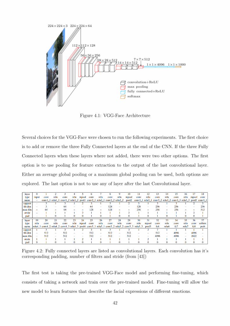
Figure 4.1: VGG-Face Architecture

Several choices for the VGG-Face were chosen to run the following experiments. The first choice

is to add or remove the three Fully Connected layers at the end of the CNN. If the three Fully

Connected layers when these layers where not added, there were two other options. The first

option is to use pooling for feature extraction to the output of the last convolutional layer.

Either an average global pooling or a maximum global pooling can be used, both options are

explored. The last option is not to use any of layer after the last Convolutional layer.

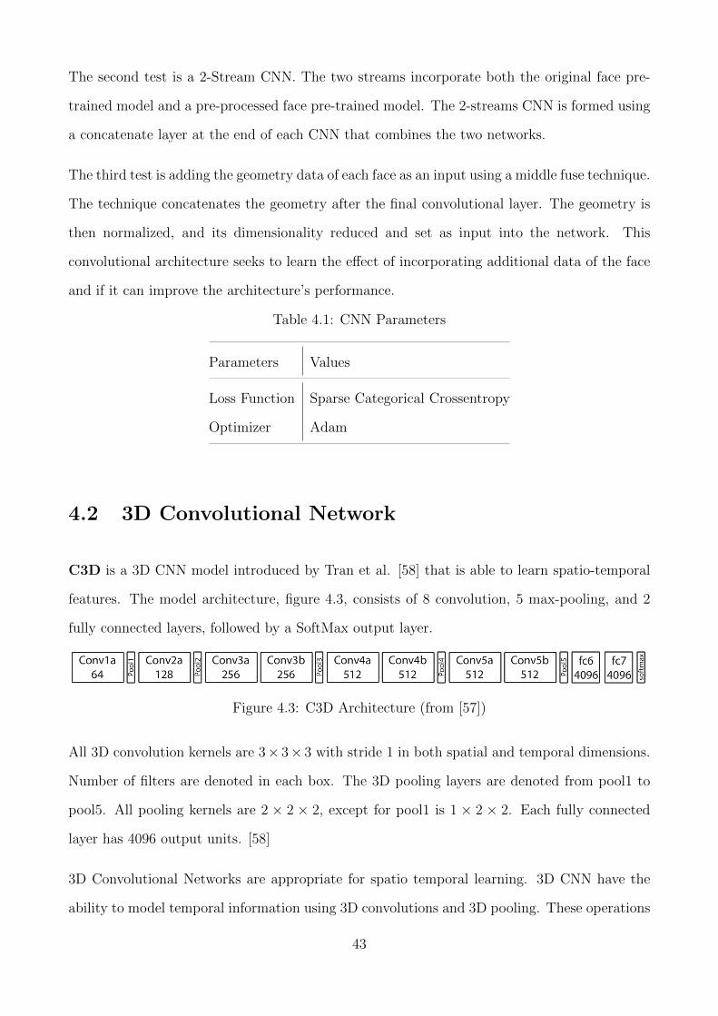
Figure 4.2: Fully connected layers are listed as convolutional layers. Each convolution has it’scorresponding padding, number of filters and stride (from [43])

The first test is taking the pre-trained VGG-Face model and performing fine-tuning, which

consists of taking a network and train over the pre-trained model. Fine-tuning will allow the

new model to learn features that describe the facial expressions of different emotions.

42

The second test is a 2-Stream CNN. The two streams incorporate both the original face pre-

trained model and a pre-processed face pre-trained model. The 2-streams CNN is formed using

a concatenate layer at the end of each CNN that combines the two networks.

The third test is adding the geometry data of each face as an input using a middle fuse technique.

The technique concatenates the geometry after the final convolutional layer. The geometry is

then normalized, and its dimensionality reduced and set as input into the network. This

convolutional architecture seeks to learn the effect of incorporating additional data of the face

and if it can improve the architecture’s performance.

Table 4.1: CNN Parameters

Parameters Values

Loss Function Sparse Categorical Crossentropy

Optimizer Adam

4.2 3D Convolutional Network

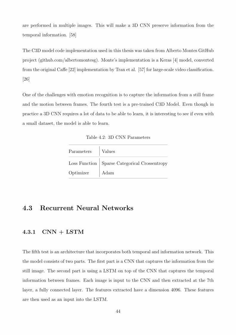
C3D is a 3D CNN model introduced by Tran et al. [58] that is able to learn spatio-temporal

features. The model architecture, figure 4.3, consists of 8 convolution, 5 max-pooling, and 2

fully connected layers, followed by a SoftMax output layer.

Figure 4.3: C3D Architecture (from [57])

All 3D convolution kernels are 3× 3× 3 with stride 1 in both spatial and temporal dimensions.

Number of filters are denoted in each box. The 3D pooling layers are denoted from pool1 to

pool5. All pooling kernels are 2 × 2 × 2, except for pool1 is 1 × 2 × 2. Each fully connected

layer has 4096 output units. [58]

3D Convolutional Networks are appropriate for spatio temporal learning. 3D CNN have the

ability to model temporal information using 3D convolutions and 3D pooling. These operations

43

are performed in multiple images. This will make a 3D CNN preserve information from the

temporal information. [58]

The C3D model code implementation used in this thesis was taken from Alberto Montes GitHub

project (github.com/albertomontesg). Monte’s implementation is a Keras [4] model, converted

from the original Caffe [22] implementation by Tran et al. [57] for large-scale video classification.

[26]

One of the challenges with emotion recognition is to capture the information from a still frame

and the motion between frames. The fourth test is a pre-trained C3D Model. Even though in

practice a 3D CNN requires a lot of data to be able to learn, it is interesting to see if even with

a small dataset, the model is able to learn.

Table 4.2: 3D CNN Parameters

Parameters Values

Loss Function Sparse Categorical Crossentropy

Optimizer Adam

4.3 Recurrent Neural Networks

4.3.1 CNN + LSTM

The fifth test is an architecture that incorporates both temporal and information network. This

the model consists of two parts. The first part is a CNN that captures the information from the

still image. The second part is using a LSTM on top of the CNN that captures the temporal

information between frames. Each image is input to the CNN and then extracted at the 7th

layer, a fully connected layer. The features extracted have a dimension 4096. These features

are then used as an input into the LSTM.

44

4.3.2 CNN + GRU

The sixth test is similar to the previous model however instead of using a LSTM, a GRU is

used. Again, this model incorporates both temporal and information network in a two-part

network. The first is a CNN and the second is a GRU on top. Each image is input to the

CNN and then extracted at the 7th layer, a fully connected layer. The features extracted have

a dimension 4096. These features are then used as an input into the GRU.

GRU is a simplified version of LSTM. It is interesting to analyse the performance between both

of them.

Table 4.3: CNN + RNN Parameters

Parameters Values

Loss Function Sparse Categorical Crossentropy

Optimizer Adam

Number of Layers 3

45

Chapter 5

Datasets

Two public datasets have been selected to test the models. Both datasets consist of videos

of various participants that perform a facial expression that characterize a series of emotions.

Both of them are used for image sequences; one is only used for hidden emotion though.

5.1 SASE-FE

The first experiments were conducted using the SASE-FE database [40]. This dataset consists

of 643 different videos. A total of 50 subjects participate. The participants have a range of age

between 19 to 36. The dataset uses the six universal expressions: Happiness, Sadness, Anger,

Disgust, Contempt and Surprise as shown in figure 5.2. Each participant in the dataset has

two facial expressions of emotions, a genuine and a deceptive, an example is depicted in figure

5.1.

46

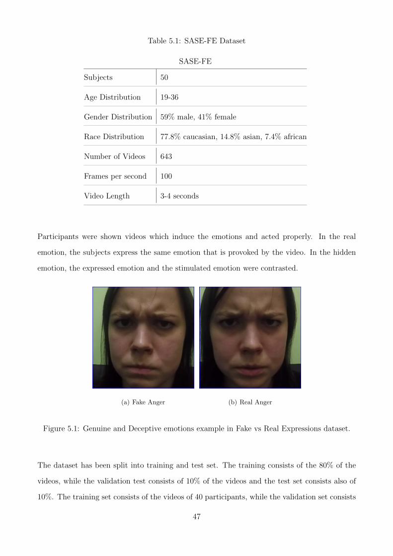
Table 5.1: SASE-FE Dataset

SASE-FE

Subjects 50

Age Distribution 19-36

Gender Distribution 59% male, 41% female

Race Distribution 77.8% caucasian, 14.8% asian, 7.4% african

Number of Videos 643

Frames per second 100

Video Length 3-4 seconds

Participants were shown videos which induce the emotions and acted properly. In the real

emotion, the subjects express the same emotion that is provoked by the video. In the hidden

emotion, the expressed emotion and the stimulated emotion were contrasted.

(a) Fake Anger (b) Real Anger

Figure 5.1: Genuine and Deceptive emotions example in Fake vs Real Expressions dataset.

The dataset has been split into training and test set. The training consists of the 80% of the

videos, while the validation test consists of 10% of the videos and the test set consists also of

10%. The training set consists of the videos of 40 participants, while the validation set consists

47

of videos of 8 participants.

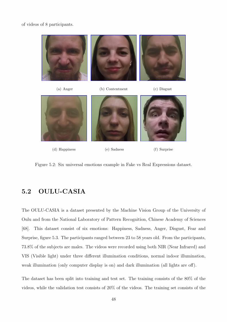
(a) Anger (b) Contentment (c) Disgust

(d) Happiness (e) Sadness (f) Surprise

Figure 5.2: Six universal emotions example in Fake vs Real Expressions dataset.

5.2 OULU-CASIA

The OULU-CASIA is a dataset presented by the Machine Vision Group of the University of

Oulu and from the National Laboratory of Pattern Recognition, Chinese Academy of Sciences

[68]. This dataset consist of six emotions: Happiness, Sadness, Anger, Disgust, Fear and

Surprise, figure 5.3. The participants ranged between 23 to 58 years old. From the participants,

73.8% of the subjects are males. The videos were recorded using both NIR (Near Infrared) and

VIS (Visible light) under three different illumination conditions, normal indoor illumination,

weak illumination (only computer display is on) and dark illumination (all lights are off).

The dataset has been split into training and test set. The training consists of the 80% of the

videos, while the validation test consists of 20% of the videos. The training set consists of the

48

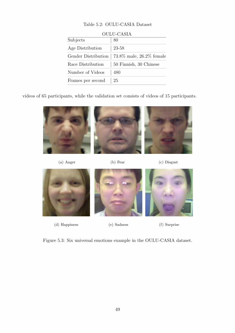
Table 5.2: OULU-CASIA Dataset

OULU-CASIASubjects 80

Age Distribution 23-58

Gender Distribution 73.8% male, 26.2% female

Race Distribution 50 Finnish, 30 Chinese

Number of Videos 480

Frames per second 25

videos of 65 participants, while the validation set consists of videos of 15 participants.

(a) Anger (b) Fear (c) Disgust

(d) Happiness (e) Sadness (f) Surprise

Figure 5.3: Six universal emotions example in the OULU-CASIA dataset.

49

Chapter 6

Setup

This section discusses the steps performed for pre-processing. Both SASE-FE and OULU-

CASIA datasets follow the same process. The non-temporal models do not accept videos as

inputs; the videos must be converted by extracting frames and using them as inputs to the

models. The temporal models receive as an input a vector consisting of a series of these frames.

6.1 Pre-processing

The videos were pre-processed to extract each frame as an image. Because the videos start with

a neutral face expression and then the participant makes the facial expression corresponding

to the emotion, there are some frames which are of no use. The pre-processing considers this

and only keep the frames from half of the video duration until the 80% of the video duration.

This ensures that the frames obtained shows the intended emotion.

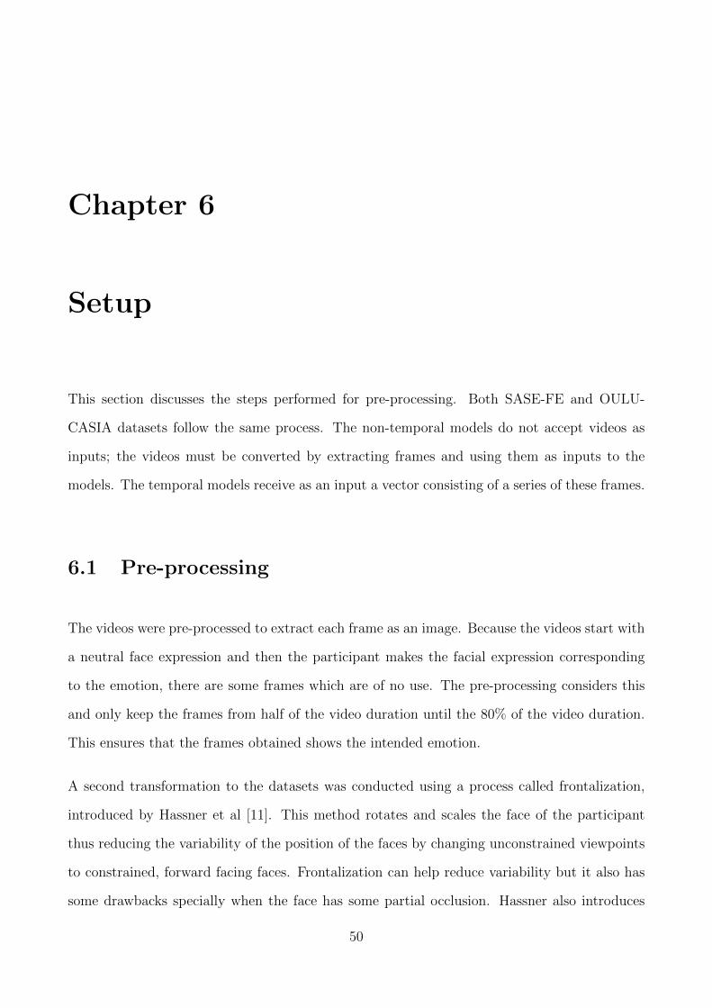
A second transformation to the datasets was conducted using a process called frontalization,

introduced by Hassner et al [11]. This method rotates and scales the face of the participant

thus reducing the variability of the position of the faces by changing unconstrained viewpoints

to constrained, forward facing faces. Frontalization can help reduce variability but it also has

some drawbacks specially when the face has some partial occlusion. Hassner also introduces

50

soft symmetry that allows occluded parts of the face to be estimated when both parts of the

face are different. Blending methods are employed obtain an image that is symmetrical on both

sides. Figure 6.1 shows an image with no symmetry and one with soft symmetry.

Figure 6.1: Right image shows an image with No Symmetry frontalization. Left image corre-sponds to a Soft Symmetry frontalization process.

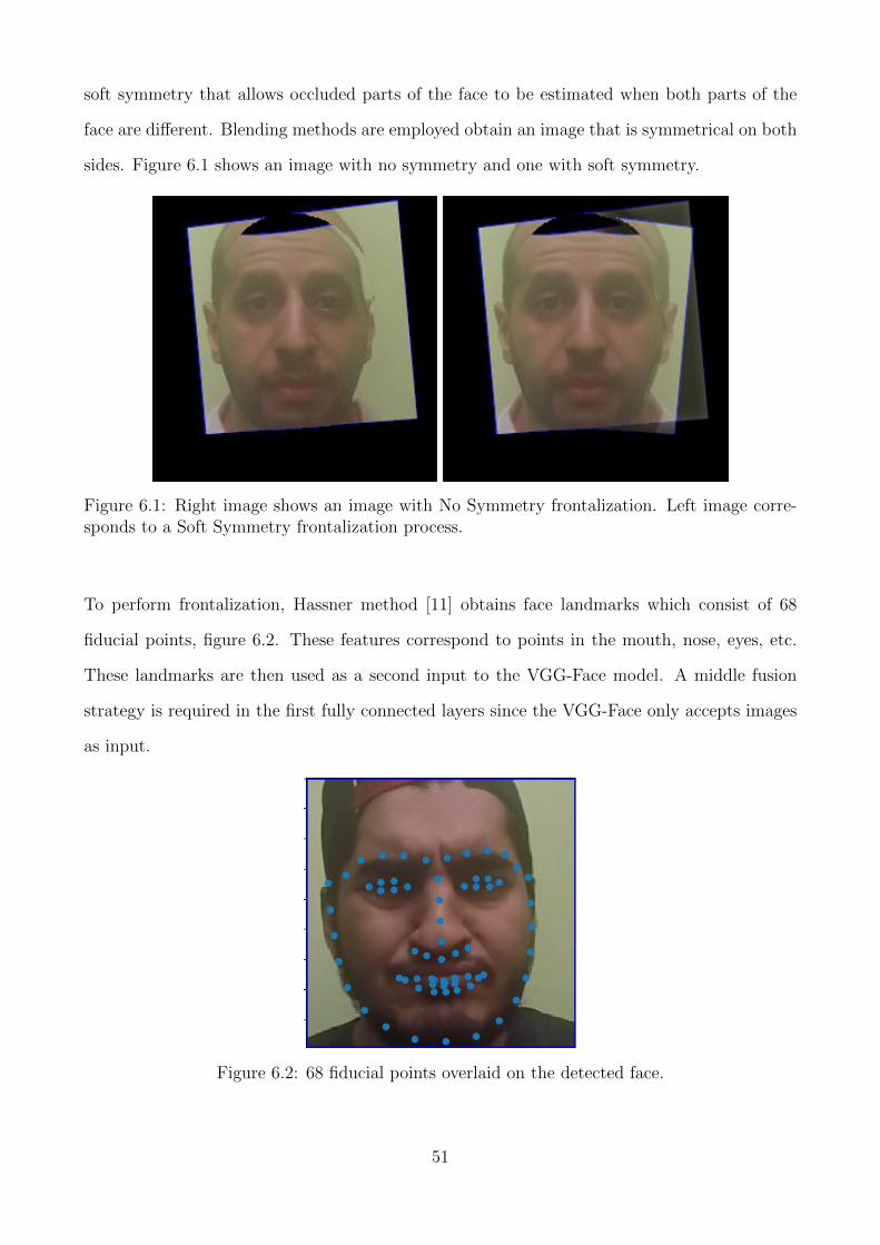
To perform frontalization, Hassner method [11] obtains face landmarks which consist of 68

fiducial points, figure 6.2. These features correspond to points in the mouth, nose, eyes, etc.

These landmarks are then used as a second input to the VGG-Face model. A middle fusion

strategy is required in the first fully connected layers since the VGG-Face only accepts images

as input.

Figure 6.2: 68 fiducial points overlaid on the detected face.

51

Chapter 7

Experimental Results

This chapter presents the results from the different experiments held on different dataset con-

figurations using different model arrangements. For general purpose, only the test accuracy is

presented.

7.1 SASE-FE Emotion Results

The first set of experiments were conducted only to classify the six emotions, both real and fake

emotions were combined. These experiments consist of doing fine-tuning to the model using

the SASE-FE dataset. The purpose is to explore different configurations and choose the model

with the highest test accuracy.

7.1.1 No Pre-Processing

The experiments try to explore if adding three fully connected layers and/or pooling

layer at the end of the convolutional layers improves the performance of the CNN. Other

experiments consist of freezing all the convolutional layers, freezing just the first few

layers and no freezing any layer.

52

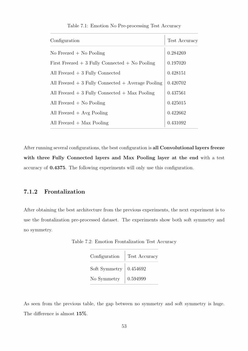
Table 7.1: Emotion No Pre-processing Test Accuracy

Configuration Test Accuracy

No Freezed + No Pooling 0.284269

First Freezed + 3 Fully Connected + No Pooling 0.197020

All Freezed + 3 Fully Connected 0.428151

All Freezed + 3 Fully Connected + Average Pooling 0.420702

All Freezed + 3 Fully Connected + Max Pooling 0.437561

All Freezed + No Pooling 0.425015

All Freezed + Avg Pooling 0.422662

All Freezed + Max Pooling 0.431092

After running several configurations, the best configuration is all Convolutional layers freeze

with three Fully Connected layers and Max Pooling layer at the end with a test

accuracy of 0.4375. The following experiments will only use this configuration.

7.1.2 Frontalization

After obtaining the best architecture from the previous experiments, the next experiment is to

use the frontalization pre-processed dataset. The experiments show both soft symmetry and

no symmetry.

Table 7.2: Emotion Frontalization Test Accuracy

Configuration Test Accuracy

Soft Symmetry 0.454692

No Symmetry 0.594999

As seen from the previous table, the gap between no symmetry and soft symmetry is huge.

The difference is almost 15%.

53

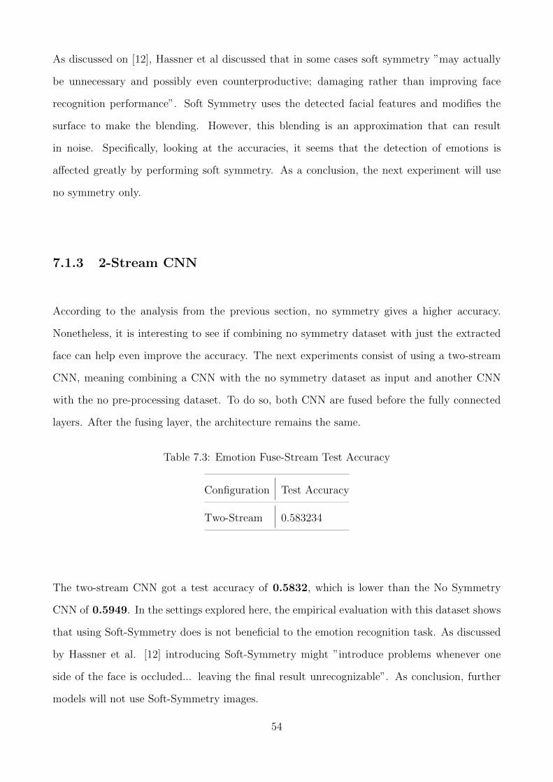
As discussed on [12], Hassner et al discussed that in some cases soft symmetry ”may actually

be unnecessary and possibly even counterproductive; damaging rather than improving face

recognition performance”. Soft Symmetry uses the detected facial features and modifies the

surface to make the blending. However, this blending is an approximation that can result

in noise. Specifically, looking at the accuracies, it seems that the detection of emotions is

affected greatly by performing soft symmetry. As a conclusion, the next experiment will use

no symmetry only.

7.1.3 2-Stream CNN

According to the analysis from the previous section, no symmetry gives a higher accuracy.

Nonetheless, it is interesting to see if combining no symmetry dataset with just the extracted

face can help even improve the accuracy. The next experiments consist of using a two-stream

CNN, meaning combining a CNN with the no symmetry dataset as input and another CNN

with the no pre-processing dataset. To do so, both CNN are fused before the fully connected

layers. After the fusing layer, the architecture remains the same.

Table 7.3: Emotion Fuse-Stream Test Accuracy

Configuration Test Accuracy

Two-Stream 0.583234

The two-stream CNN got a test accuracy of 0.5832, which is lower than the No Symmetry

CNN of 0.5949. In the settings explored here, the empirical evaluation with this dataset shows

that using Soft-Symmetry does is not beneficial to the emotion recognition task. As discussed

by Hassner et al. [12] introducing Soft-Symmetry might ”introduce problems whenever one

side of the face is occluded... leaving the final result unrecognizable”. As conclusion, further

models will not use Soft-Symmetry images.

54

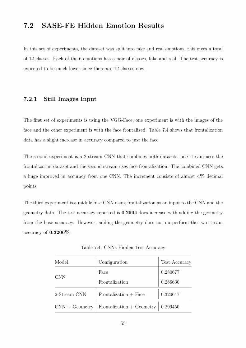
7.2 SASE-FE Hidden Emotion Results

In this set of experiments, the dataset was split into fake and real emotions, this gives a total

of 12 classes. Each of the 6 emotions has a pair of classes, fake and real. The test accuracy is

expected to be much lower since there are 12 classes now.

7.2.1 Still Images Input

The first set of experiments is using the VGG-Face, one experiment is with the images of the

face and the other experiment is with the face frontalized. Table 7.4 shows that frontalization

data has a slight increase in accuracy compared to just the face.

The second experiment is a 2 stream CNN that combines both datasets, one stream uses the

frontalization dataset and the second stream uses face frontalization. The combined CNN gets

a huge improved in accuracy from one CNN. The increment consists of almost 4% decimal

points.

The third experiment is a middle fuse CNN using frontalization as an input to the CNN and the

geometry data. The test accuracy reported is 0.2994 does increase with adding the geometry

from the base accuracy. However, adding the geometry does not outperform the two-stream

accuracy of 0.3206%.

Table 7.4: CNNs Hidden Test Accuracy

Model Configuration Test Accuracy

CNNFace 0.280677

Frontalization 0.286630

2-Stream CNN Frontalization + Face 0.320647

CNN + Geometry Frontalization + Geometry 0.299450

55

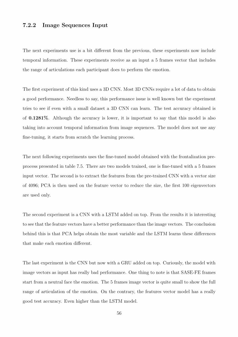
7.2.2 Image Sequences Input

The next experiments use is a bit different from the previous, these experiments now include

temporal information. These experiments receive as an input a 5 frames vector that includes

the range of articulations each participant does to perform the emotion.

The first experiment of this kind uses a 3D CNN. Most 3D CNNs require a lot of data to obtain

a good performance. Needless to say, this performance issue is well known but the experiment

tries to see if even with a small dataset a 3D CNN can learn. The test accuracy obtained is

of 0.1281%. Although the accuracy is lower, it is important to say that this model is also

taking into account temporal information from image sequences. The model does not use any

fine-tuning, it starts from scratch the learning process.

The next following experiments uses the fine-tuned model obtained with the frontalization pre-

process presented in table 7.5. There are two models trained, one is fine-tuned with a 5 frames

input vector. The second is to extract the features from the pre-trained CNN with a vector size

of 4096; PCA is then used on the feature vector to reduce the size, the first 100 eigenvectors

are used only.

The second experiment is a CNN with a LSTM added on top. From the results it is interesting

to see that the feature vectors have a better performance than the image vectors. The conclusion

behind this is that PCA helps obtain the most variable and the LSTM learns these differences

that make each emotion different.

The last experiment is the CNN but now with a GRU added on top. Curiously, the model with

image vectors as input has really bad performance. One thing to note is that SASE-FE frames

start from a neutral face the emotion. The 5 frames image vector is quite small to show the full

range of articulation of the emotion. On the contrary, the features vector model has a really

good test accuracy. Even higher than the LSTM model.

56

Table 7.5: Temporal Hidden Test Accuracy

Model Configuration Test Accuracy

3D CNN Frontalization 0.128125

CNN + LSTMFeatures 0.159200

Image 0.148684

CNN + GRUFeatures 0.183311

Image 0.084134

7.3 OULU-CASIA Results

The following set of experiments were conducted only to classify the six emotions of the OULU-

CASIA dataset.

7.3.1 Still Images Input

The first set of experiments consists of first fine-tuning the VGG-Face with the images without

any pre-processing; the other experiment is performed using the frontalization pre-processed

images. The pre-processed images outperformed the non-processing images with almost 0.03%.

This pre-processing does improve the accuracy of the models. This is because the frontalization

normalizes the faces and helps the model learn better the differences of the emotions; by

normalizing the images data loses noise so in this case the performance receives an increase in

accuracy.

The second experiment uses a 2-Stream CNN, which tries to see if adding both the face and

the frontalization datasets improves the accuracy of the previous two experiments. From the

previous experiments, the frontalization got a 0.2659%. The two stream CNN outperform the

model with a higher score of 0.2737%. This makes sure that the model learns all the informa-

tion possible from the face, even information that might have been lost from the frontalization

57

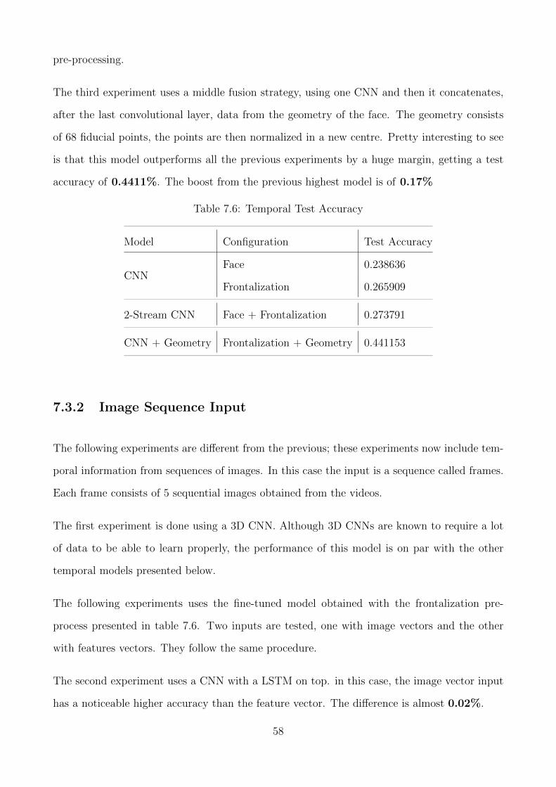
pre-processing.

The third experiment uses a middle fusion strategy, using one CNN and then it concatenates,

after the last convolutional layer, data from the geometry of the face. The geometry consists

of 68 fiducial points, the points are then normalized in a new centre. Pretty interesting to see

is that this model outperforms all the previous experiments by a huge margin, getting a test

accuracy of 0.4411%. The boost from the previous highest model is of 0.17%

Table 7.6: Temporal Test Accuracy

Model Configuration Test Accuracy

CNNFace 0.238636

Frontalization 0.265909

2-Stream CNN Face + Frontalization 0.273791

CNN + Geometry Frontalization + Geometry 0.441153

7.3.2 Image Sequence Input

The following experiments are different from the previous; these experiments now include tem-

poral information from sequences of images. In this case the input is a sequence called frames.

Each frame consists of 5 sequential images obtained from the videos.

The first experiment is done using a 3D CNN. Although 3D CNNs are known to require a lot

of data to be able to learn properly, the performance of this model is on par with the other

temporal models presented below.

The following experiments uses the fine-tuned model obtained with the frontalization pre-

process presented in table 7.6. Two inputs are tested, one with image vectors and the other

with features vectors. They follow the same procedure.

The second experiment uses a CNN with a LSTM on top. in this case, the image vector input

has a noticeable higher accuracy than the feature vector. The difference is almost 0.02%.

58

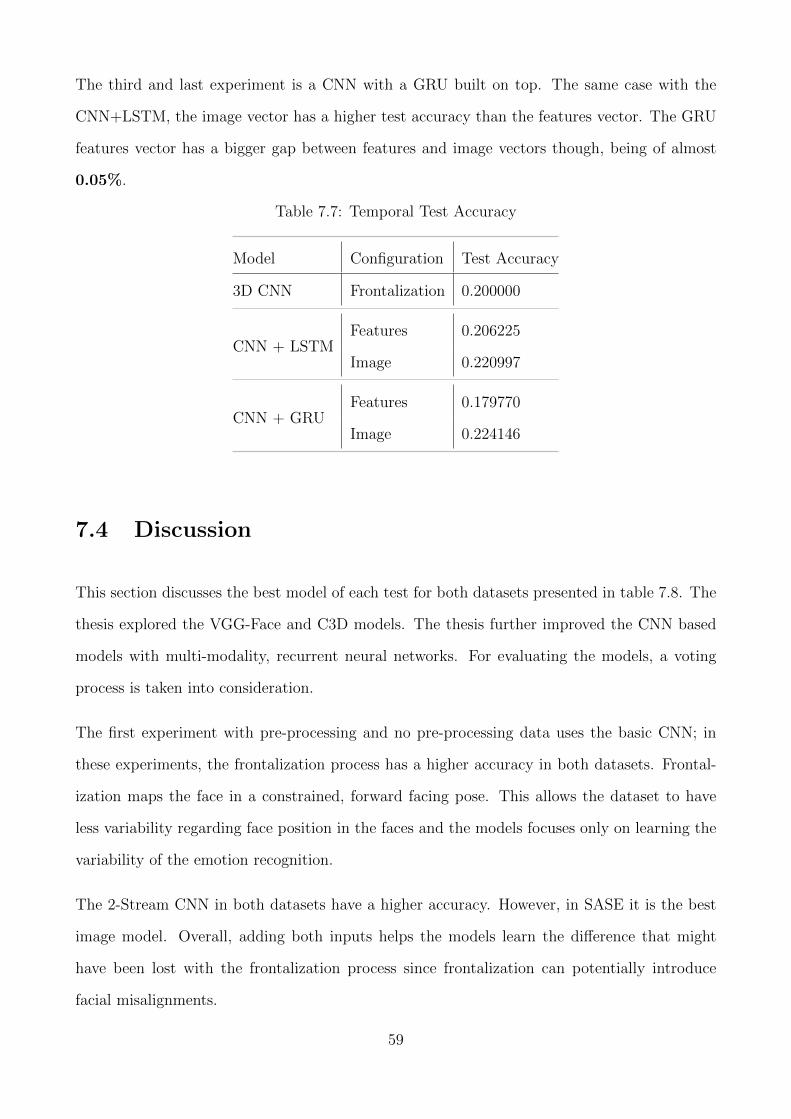
The third and last experiment is a CNN with a GRU built on top. The same case with the

CNN+LSTM, the image vector has a higher test accuracy than the features vector. The GRU

features vector has a bigger gap between features and image vectors though, being of almost

0.05%.

Table 7.7: Temporal Test Accuracy

Model Configuration Test Accuracy

3D CNN Frontalization 0.200000

CNN + LSTMFeatures 0.206225

Image 0.220997

CNN + GRUFeatures 0.179770

Image 0.224146

7.4 Discussion

This section discusses the best model of each test for both datasets presented in table 7.8. The

thesis explored the VGG-Face and C3D models. The thesis further improved the CNN based

models with multi-modality, recurrent neural networks. For evaluating the models, a voting

process is taken into consideration.

The first experiment with pre-processing and no pre-processing data uses the basic CNN; in

these experiments, the frontalization process has a higher accuracy in both datasets. Frontal-

ization maps the face in a constrained, forward facing pose. This allows the dataset to have

less variability regarding face position in the faces and the models focuses only on learning the

variability of the emotion recognition.

The 2-Stream CNN in both datasets have a higher accuracy. However, in SASE it is the best

image model. Overall, adding both inputs helps the models learn the difference that might

have been lost with the frontalization process since frontalization can potentially introduce

facial misalignments.

59

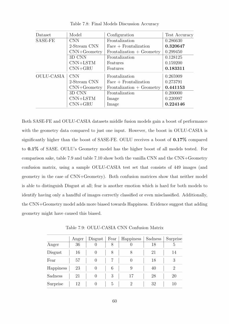
Table 7.8: Final Models Discussion Accuracy

Dataset Model Configuration Test AccuracySASE-FE CNN Frontalization 0.286630

2-Stream CNN Face + Frontalization 0.320647CNN+Geometry Frontalization + Geometry 0.2994503D CNN Frontalization 0.128125CNN+LSTM Features 0.159200CNN+GRU Features 0.183311

OULU-CASIA CNN Frontalization 0.2659092-Stream CNN Face + Frontalization 0.273791CNN+Geometry Frontalization + Geometry 0.4411533D CNN Frontalization 0.200000CNN+LSTM Image 0.220997CNN+GRU Image 0.224146

Both SASE-FE and OULU-CASIA datasets middle fusion models gain a boost of performance

with the geometry data compared to just one input. However, the boost in OULU-CASIA is

significantly higher than the boost of SASE-FE. OULU receives a boost of 0.17% compared

to 0.1% of SASE. OULU’s Geometry model has the higher boost of all models tested. For

comparison sake, table 7.9 and table 7.10 show both the vanilla CNN and the CNN+Geometry

confusion matrix, using a sample OULU-CASIA test set that consists of 449 images (and

geometry in the case of CNN+Geometry). Both confusion matrices show that neither model

is able to distinguish Disgust at all; fear is another emotion which is hard for both models to

identify having only a handful of images correctly classified or even misclassified. Additionally,

the CNN+Geometry model adds more biased towards Happiness. Evidence suggest that adding

geometry might have caused this biased.

Table 7.9: OULU-CASIA CNN Confusion Matrix

Anger Disgust Fear Happiness Sadness SurpriseAnger 36 0 8 0 18 5

Disgust 16 0 8 8 21 14

Fear 57 0 7 0 18 3

Happiness 23 0 6 9 40 2

Sadness 21 0 3 17 28 20

Surprise 12 0 5 2 32 10

60

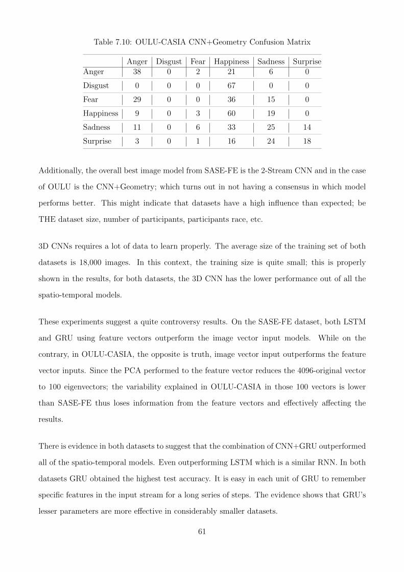
Table 7.10: OULU-CASIA CNN+Geometry Confusion Matrix

Anger Disgust Fear Happiness Sadness SurpriseAnger 38 0 2 21 6 0

Disgust 0 0 0 67 0 0

Fear 29 0 0 36 15 0

Happiness 9 0 3 60 19 0

Sadness 11 0 6 33 25 14

Surprise 3 0 1 16 24 18

Additionally, the overall best image model from SASE-FE is the 2-Stream CNN and in the case

of OULU is the CNN+Geometry; which turns out in not having a consensus in which model

performs better. This might indicate that datasets have a high influence than expected; be

THE dataset size, number of participants, participants race, etc.

3D CNNs requires a lot of data to learn properly. The average size of the training set of both

datasets is 18,000 images. In this context, the training size is quite small; this is properly

shown in the results, for both datasets, the 3D CNN has the lower performance out of all the

spatio-temporal models.

These experiments suggest a quite controversy results. On the SASE-FE dataset, both LSTM

and GRU using feature vectors outperform the image vector input models. While on the

contrary, in OULU-CASIA, the opposite is truth, image vector input outperforms the feature

vector inputs. Since the PCA performed to the feature vector reduces the 4096-original vector

to 100 eigenvectors; the variability explained in OULU-CASIA in those 100 vectors is lower

than SASE-FE thus loses information from the feature vectors and effectively affecting the

results.

There is evidence in both datasets to suggest that the combination of CNN+GRU outperformed

all of the spatio-temporal models. Even outperforming LSTM which is a similar RNN. In both

datasets GRU obtained the highest test accuracy. It is easy in each unit of GRU to remember

specific features in the input stream for a long series of steps. The evidence shows that GRU’s

lesser parameters are more effective in considerably smaller datasets.

61

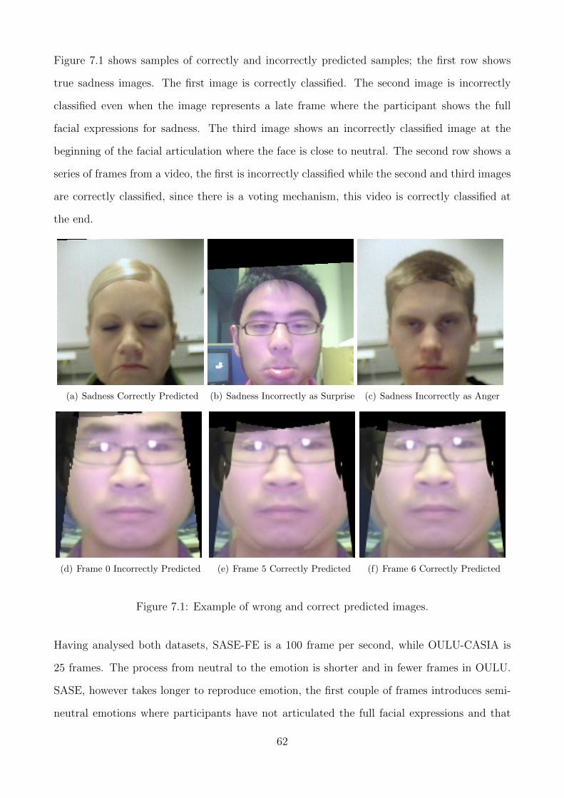
Figure 7.1 shows samples of correctly and incorrectly predicted samples; the first row shows

true sadness images. The first image is correctly classified. The second image is incorrectly

classified even when the image represents a late frame where the participant shows the full

facial expressions for sadness. The third image shows an incorrectly classified image at the

beginning of the facial articulation where the face is close to neutral. The second row shows a

series of frames from a video, the first is incorrectly classified while the second and third images

are correctly classified, since there is a voting mechanism, this video is correctly classified at

the end.

(a) Sadness Correctly Predicted (b) Sadness Incorrectly as Surprise (c) Sadness Incorrectly as Anger

(d) Frame 0 Incorrectly Predicted (e) Frame 5 Correctly Predicted (f) Frame 6 Correctly Predicted

Figure 7.1: Example of wrong and correct predicted images.

Having analysed both datasets, SASE-FE is a 100 frame per second, while OULU-CASIA is

25 frames. The process from neutral to the emotion is shorter and in fewer frames in OULU.

SASE, however takes longer to reproduce emotion, the first couple of frames introduces semi-

neutral emotions where participants have not articulated the full facial expressions and that

62

could have introduced noise into the learning models.

Overall, still images models have a higher accuracy than image sequences models. Although

there is evidence to say that temporal features are not as important, temporal models require

huge amount of data to be able to generalize compared to still images; having said that, there

is not sufficient evidence to conclude if temporal models perform worse given the small size of

both datasets.

63

Chapter 8

Conclusion

In this thesis, it is empirically evaluated deep learning models including CNNs, 3D CNNs and

RNNs. The evaluation focuses on the task of emotion recognition through facial expression

in image sequences on a number of datasets including SASE-FE and OULU-CASIA. These

datasets provide data for six basic emotions, presented in a series of videos, that were used, one

for emotion classification and the other for real and hidden emotions using image sequences.

The evaluation clearly demonstrated the superiority of performing face frontalization for pre-

processing the data over performing no pre-processing at all.

The basic model was further improved using multi-modal models using the geometry data of

the face. In addition, using a 2-Stream CNN further improved the base model. In spite the

fact that both improved the base model, there was no clear consensus which model improved

to a greater extent the base model.

A 3D CNN model was considered in the experiment and it was successfully shown their useful-

ness in emotion recognition. Moreover, it was demonstrated the superiority of the GRU models

in image-sequence inputs over the 3D CNN and LSTM spatio-temporal models. However, it

was not possible to concretely conclude if using extracted feature vectors from the CNN as the

input of the RNNs were better than using image vectors as inputs.

64

8.0.1 Future Work

In the work for this thesis, deep learning models were trained with pre-processed images that

aligned the face and resolve occlusion. To further improve the model, it is compulsory to focus

on adding deep characteristics around the face’s points of interest.

Also, it is compelling to include more data using more databases as most temporal models

require lots of data for training. This thesis uses the VGG-Face, future work would try other

pre-trained models such as LeNet, AlexNet, etc.

Moreover, it would be interesting to combine deep architectures with hand-crafted features that

combine spatio-temporal features like spatio-temporal interest points (STIPS), histograms of

optical flow (HOF), motion boundary histograms (MBH), etc.

65

Bibliography

[1] F. P. Bengio Yoshua, Simard Patrice. Learning Long-Term Dependencies with Gradient

Descent is Difficult. IEEE Transactions on Neural Networks, 5(2):157 – 166, 1994.

[2] M. G. Calvo and D. Lundqvist. Facial expressions of emotion (KDEF): Identification under

different display-duration conditions. Behavior Research Methods, 2008.

[3] K. Cho, B. Van Merrienboer, C. Gulcehre, D. Bahdanau, F. Bougares, H. Schwenk, and

Y. Bengio. Learning Phrase Representations using RNN EncoderDecoder for Statistical

Machine Translation.

[4] F. Chollet et al. Keras, 2015.

[5] J. Chung, C. Gulcehre, and K. Cho. Empirical Evaluation of Gated Recurrent Neural

Networks on Sequence Modeling.

[6] N. Dalal and B. Triggs. Histograms of oriented gradients for human detection. In Pro-

ceedings - 2005 IEEE Computer Society Conference on Computer Vision and Pattern

Recognition, CVPR 2005, 2005.

[7] A. Dhall, O. V. Ramana Murthy, R. Goecke, J. Joshi, and T. Gedeon. Video and image

based emotion recognition challenges in the wild: Emotiw 2015. Proceedings of the 2015

ACM on International Conference on Multimodal Interaction, 2015.

[8] C. Feichtenhofer, A. Pinz, and A. Zisserman. Convolutional Two-Stream Network Fusion

for Video Action Recognition. 2016.

[9] Goodfellow. Ian, Y. Bengio, and A. Courville. Deep Learning. MIT Press, 2016.

66

[10] D. J. Hand, H. Mannila, and P. Smyth. Principles of Data Mining. The MIT Press,

Cambridge, Massachusetts, 1st edition, 2001.

[11] T. Hassner, S. Harel, E. Paz, and R. Enbar. Effective Face Frontalization in Unconstrained

Images.

[12] T. Hassner, S. Harel, E. Paz, and R. Enbar. Effective face frontalization in unconstrained

images. In Proceedings of the IEEE Computer Society Conference on Computer Vision

and Pattern Recognition, 2015.

[13] T. Hastie, R. Tibshirani, and J. Friedman. Springer Series in Statistics The Elements of

Statistical Learning The Elements of Statistical Learning.

[14] T. Hastie, R. Tibshirani, and J. Friedman. Elements of Statistical Learning. Elements,

2009.

[15] G. Hinton, N. Srivastava, and K. Swersky. Neural Networks for Machine Learning Lecture

6a Overview of mini-batch gradient descent.

[16] S. Hochreiter and J. Urgen Schmidhuber. LONG SHORT-TERM MEMORY. Neural

Computation, 9(8):1735–1780, 1997.

[17] C. Hu, J. T. Kwok, and W. Pan. Adaptive Subgradient Methods for Online Learning and

Stochastic Optimization. Science And Technology, 2011.

[18] G. B. Huang, M. Ramesh, T. Berg, and E. Learned-Miller. Labeled Faces in the Wild: A

Database for Studying Face Recognition in Unconstrained Environments.

[19] D. H. Hubel and T. N. Wiesel. Receptive fields and functional architecture of monkey

striate cortex. J. Physiol., 1968.

[20] K. Janocha and W. M. Czarnecki. On Loss Functions for Deep Neural Networks in Clas-

sification. Schedae Informaticae, 2017.

[21] S. Ji, W. Xu, M. Yang, and K. Yu. 3D Convolutional Neural Networks for Human Action

Recognition.

67

[22] Y. Jia, E. Shelhamer, J. Donahue, S. Karayev, J. Long, R. Girshick, S. Guadarrama, and

T. Darrell. Caffe: Convolutional Architecture for Fast Feature Embedding *.

[23] T. Kanade, J. F. Cohn, and Y. Tian. Comprehensive Database for Facial Expression

Analysis.

[24] U. Karn. A Quick Introduction to Neural Networks.

[25] A. Karpath. CS231n Convolutional Neural Networks for Visual Recognition, 2018.

[26] A. Karpathy, G. Toderici, S. Shetty, T. Leung, R. Sukthankar, and L. Fei-Fei. Large-scale

Video Classication with Convolutional Neural Networks. In Large-scale Video Classication

with Convolutional Neural Networks, 2014.

[27] D. P. Kingma and J. Ba. Adam: A Method for Stochastic Optimization. In The 3rd

International Conference for Learning Representations, 2015.

[28] A. Krizhevsky. Learning Multiple Layers of Features from Tiny Images. 2009.

[29] A. Krizhevsky, I. Sutskever, and G. E. Hinton. ImageNet Classification with Deep Convo-

lutional Neural Networks.

[30] A. Krizhevsky, I. Sutskever, and G. E. Hinton. ImageNet Classification with Deep Convo-

lutional Neural Networks.

[31] Y. LeCun, L. Bottou, Y. Bengio, and P. Haffner. Gradient-based learning applied to

document recognition. Proceedings of the IEEE, 1998.

[32] Y. LeCun and C. Cortes. MNIST handwritten digit database. AT&T Labs [Online].

Available: http://yann. lecun. com/exdb/mnist, 2010.

[33] P. Liu and L. Yin. Spontaneous Thermal Facial Expression Analysis Based On Trajectory-

Pooled Fisher Vector Descriptor.

[34] P. Lucey, J. F. Cohn, T. Kanade, J. Saragih, Z. Ambadar, and I. Matthews. The Extended

Cohn-Kanade Dataset (CK+): A complete dataset for action unit and emotion-specified

expression.

68

[35] M. Lyons, S. Akamatsu, M. Kamachi, and J. Gyoba. Coding Facial Expressions with

Gabor Wavelets.

[36] S. M. Mavadati, M. H. Mahoor, K. Bartlett, P. Trinh, and J. F. Cohn. DISFA: A sponta-

neous facial action intensity database. IEEE Transactions on Affective Computing, 2013.

[37] W. S. Mcculloch and W. Pitts. A LOGICAL CALCULUS OF THE IDEAS IMMANENT

IN NERVOUS ACTIVITY*. Bulletin of Mothemnticnl Biology, 52(l2):99–115, 1990.

[38] K. P. Murphy. Machine Learning: A Probabilistic Perspective. The MIT Press, Cambridge,

Massachusetts, 1st edition, 2012.

[39] N. Neverova, C. Wolf, G. Taylor, and F. Nebout. ModDrop: Adaptive multi-modal gesture

recognition. IEEE Transactions on Pattern Analysis and Machine Intelligence, 2016.

[40] I. Ofodile, K. Kulkarni, C. A. Corneanu, S. Escalera, X. Baro, S. Hyniewska, J. Allik, and

G. Anbarjafari. Automatic Recognition of Deceptive Facial Expressions of Emotion. 2017.

[41] Olah Christopher. Understanding LSTM Networks, 2015.

[42] M. Osadchy, Le Cun. Yann, and M. L. Miller. Synergistic Face Detection and Pose Esti-

mation with Energy-Based Models. The Journal of Machine Learning Research, 2007.

[43] O. M. Parkhi, A. Vedaldi, and A. Zisserman. Deep Face Recognition. In Procedings of the

British Machine Vision Conference 2015, 2015.

[44] H. Ranganathan, S. Chakraborty, and S. Panchanathan. Multimodal Emotion Recognition

using Deep Learning Architectures.

[45] N. Ronghe, S. Nakashe, A. Pawar, and S. Bobde. Emotion recognition and reaction pre-

diction in videos, 2017.

[46] F. Rosenblatt. THE PERCEPTRON: A PROBABILISTIC MODEL FOR INFOR-

MATION STORAGE AND ORGANIZATION IN THE BRAIN. Psychological Review,

65(6):19–8.

[47] S. Ruder. An overview of gradient descent optimization algorithms. 9 2016.

69

[48] A. Ruiz-Garcia, M. Elshaw, A. Altahhan, and V. Palade. Stacked Deep Convolutional

Auto-Encoders for Emotion Recognition from Facial Expressions.

[49] D. E. Rumelhart, G. E. Hinton, and R. J. Williams. Learning Internal Representations by

Error Propagation, 1986.

[50] N. Sarode and S. Bhatia. Facial Expression Recognition. International Journal on Com-

puter Science and Engineering, 02(05):1552–1557, 2010.

[51] A. Saxena. Convolutional Neural Networks (CNNs): An Illustrated Explanation, 2016.

[52] A. Sharma V. Understanding Activation Functions in Neural Networks.

[53] P. Y. Simard, D. Steinkraus, and J. C. Platt. Best Practices for Convolutional Neural

Networks Applied to Visual Document Analysis.

[54] N. Singh Gill. Overview and Applications of Artificial Neural Networks.

[55] N. Srivastava, G. Hinton, A. Krizhevsky, I. Sutskever, and R. Salakhutdinov. Dropout: A

Simple Way to Prevent Neural Networks from Overfitting. Journal of Machine Learning

Research, 15:1929–1958, 2014.

[56] R. S. Sutton. Two problems with backpropagation and other steepest-descent learning

procedures for networks, 1986.

[57] D. Tran, L. Bourdev, R. Fergus, L. Torresani, and M. Paluri. Learning spatiotempo-

ral features with 3D convolutional networks. In Proceedings of the IEEE International

Conference on Computer Vision, 2015.

[58] D. Tran, L. Bourdev, R. Fergus, L. Torresani, and M. Paluri. Learning spatiotempo-

ral features with 3D convolutional networks. In Proceedings of the IEEE International

Conference on Computer Vision, 2015.

[59] H. C. Vijay Lakshmi and S. PatilKulakarni. Segmentation Algorithm for Multiple Face

Detection in Color Images with Skin Tone Regions using Color Spaces and Edge Detec-

tion Techniques. IEEE Signal Acquisition and Processing, 2010. ICSAP’10. International

Conference on, pages 162–166, 2010.

70

[60] P. Viola and M. Jones. Rapid object detection using a boosted cascade of simple features.

In Proceedings of the 2001 IEEE Computer Society Conference on Computer Vision and

Pattern Recognition. CVPR 2001.

[61] J. Wang and L. Perez. The Effectiveness of Data Augmentation in Image Classification

using Deep Learning.

[62] S. Wang, Z. Liu, S. Lv, Y. Lv, G. Wu, P. Peng, F. Chen, and X. Wang. A natural visible

and infrared facial expression database for expression recognition and emotion inference.

IEEE Transactions on Multimedia, 2010.

[63] P. Werbos. Beyond Regression: New Tools for Prediction and Analysis in the Behavioral

Sciences. PhD thesis, 1974.

[64] I. H. Witten, E. Frank, and M. A. Hall. Data Mining: Practical Machine Learning Tools

and Techniques. Morgan Kaufmann Publishers Inc., 3rd edition, 2011.

[65] L. Wolf, T. Hassner, and I. Maoz. Face Recognition in Unconstrained Videos with Matched

Background Similarity.

[66] D. Yi, Z. Lei, S. Liao, and S. Z. Li. Learning Face Representation from Scratch. 11 2014.

[67] M. D. Zeiler. ADADELTA: An Adaptive Learning Rate Method. 2012.

[68] G. Zhao, X. Huang, M. Taini, S. Z. Li, and M. Pietikainen. Facial expression recognition

from near-infrared videos. Image and Vision Computing, 2011.

71