Deep Representation Learning for Trajectory Similarity

Deep Representation Learning for TrajectorySimilarity Computation

Xiucheng Li†, Kaiqi Zhao†, Gao Cong†, Christian S. Jensen‡, Wei Wei◦

† Nanyang Technological Univeristy, ‡ Aalborg University, ◦ Huazhong University of Science and Technology{xli055@e., kzhao002@e., gaocong@}ntu.edu.sg, [email protected], [email protected]

Abstract—Trajectory similarity computation is fundamentalfunctionality with many applications such as animal migrationpattern studies and vehicle trajectory mining to identify popularroutes and similar drivers. While a trajectory is a continu-ous curve in some spatial domain, e.g., 2D Euclidean space,trajectories are often represented by point sequences. Existingapproaches that compute similarity based on point matchingsuffer from the problem that they treat two different pointsequences differently even when the sequences represent thesame trajectory. This is particularly a problem when the pointsequences are non-uniform, have low sampling rates, and havenoisy points. We propose the first deep learning approach tolearning representations of trajectories that is robust to lowdata quality, thus supporting accurate and efficient trajectorysimilarity computation and search. Experiments show that ourmethod is capable of higher accuracy and is at least one order ofmagnitude faster than the state-of-the-art methods for k-nearesttrajectory search.

I. INTRODUCTION

With the proliferation of GPS-enabled devices, trajectorydata is being generated at an unprecedented speed. A trajectoryis typically represented as a sequence of discrete locations,or sample points, which describes the underlying route of amoving object over time. Quantifying the similarity betweentwo trajectories is a fundamental research problem and isa foundation for many trajectory based applications, suchas tracking migration patterns of animals [1], mining hotroutes in cities [2], trajectory clustering [3] and moving groupdiscovery [4], [5]. The importance of measuring trajectorysimilarity has also been recognized by researchers, and anumber of classic methods have been proposed, such asdynamic time wrapping (DTW) [6], longest common subse-quence (LCSS) [7], edit distance with real penalty (ERP) [8],and edit distance on real sequences (EDR) [9].

These existing methods usually try to form a pairwisematching the sample points of two trajectories and iden-tify the best alignment using dynamic programming. Morespecifically, these pairwise point-matching methods implicitlypartition the space into cells according to a threshold ε andmatch two points if they fall into the same cell. Dynamicprogramming is then used to find an alignment that minimizesa matching cost.

The pairwise point-matching methods for computing trajec-tory similarity often suffer in three scenarios: the first is whenthe sampling rates of trajectories are non-uniform. Samplingrates often vary across devices due to different device settings,battery constraints, and communication failures. Even for the

same device, the sampling rates may vary. For example, a taxidriver may alter the default device sampling rate to reducethe power consumption [10]. This may result in samplingpoints alternating between sparse and dense episodes. Thisposes challenges to the existing methods—if two trajectoriesrepresent the same underlying route, but are generated atdifferent sampling rates, it is difficult for these methods toidentify them as similar trajectories. The second scenariowhere it is challenging to align the sample points of similartrajectories is when the sampling rate is low. For example, thesampling rates for trajectories generated from online “check-ins” (e.g., Foursquare, Facebook), geo-tagged tweets, geo-tagged photo albums, and call detail records are low andinherently non-uniform [11]. Third, the performance of thesemethods may be degraded when the sample points are noisy.Such noise may occur in GPS points when moving in urbancanyons.

Moreover, the existing methods rely on local point matchingand identify an optimal alignment using dynamic program-ming, which leads to quadratic computational complexityO(n2), where n is the mean length of the trajectories. Weargue that a good trajectory similarity measure should be bothaccurate and scalable to large datasets.

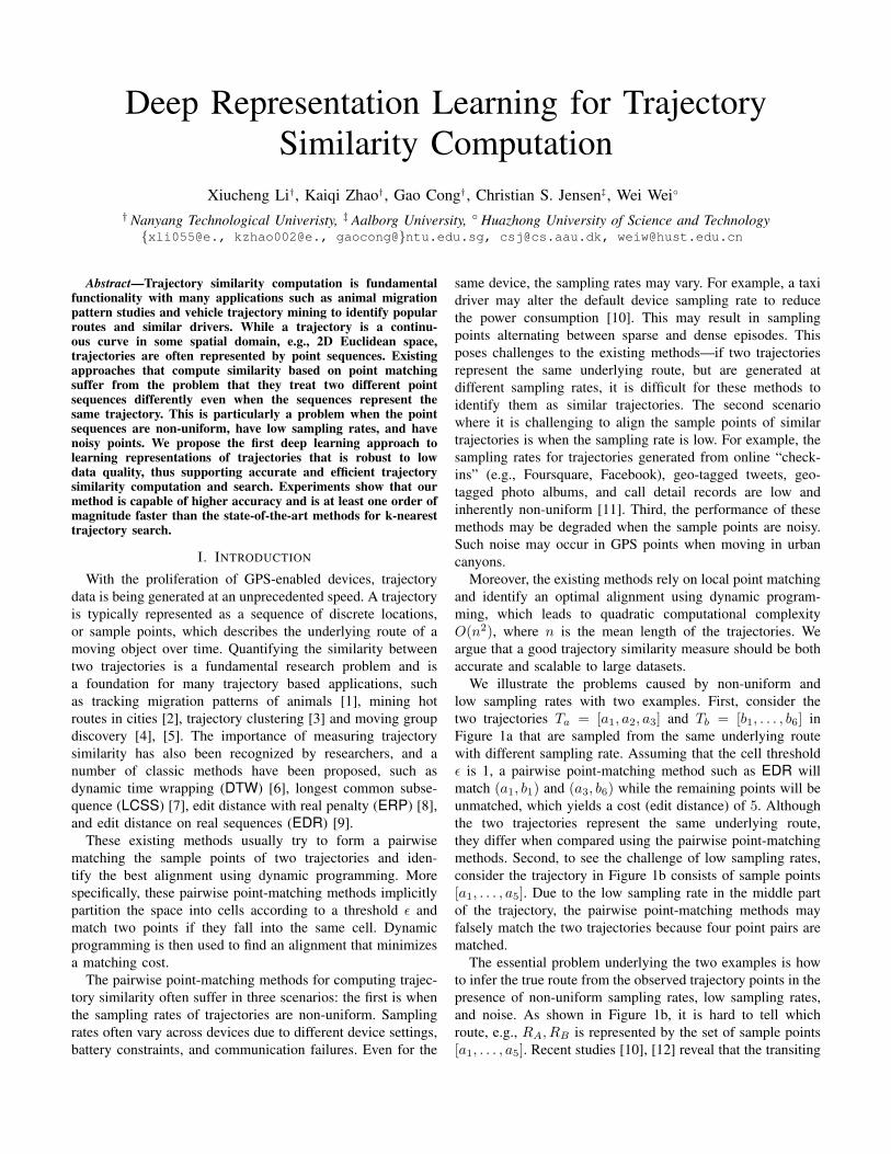
We illustrate the problems caused by non-uniform andlow sampling rates with two examples. First, consider thetwo trajectories Ta = [a1, a2, a3] and Tb = [b1, . . . , b6] inFigure 1a that are sampled from the same underlying routewith different sampling rate. Assuming that the cell thresholdε is 1, a pairwise point-matching method such as EDR willmatch (a1, b1) and (a3, b6) while the remaining points will beunmatched, which yields a cost (edit distance) of 5. Althoughthe two trajectories represent the same underlying route,they differ when compared using the pairwise point-matchingmethods. Second, to see the challenge of low sampling rates,consider the trajectory in Figure 1b consists of sample points[a1, . . . , a5]. Due to the low sampling rate in the middle partof the trajectory, the pairwise point-matching methods mayfalsely match the two trajectories because four point pairs arematched.

The essential problem underlying the two examples is howto infer the true route from the observed trajectory points in thepresence of non-uniform sampling rates, low sampling rates,and noise. As shown in Figure 1b, it is hard to tell whichroute, e.g., RA, RB is represented by the set of sample points[a1, . . . , a5]. Recent studies [10], [12] reveal that the transiting

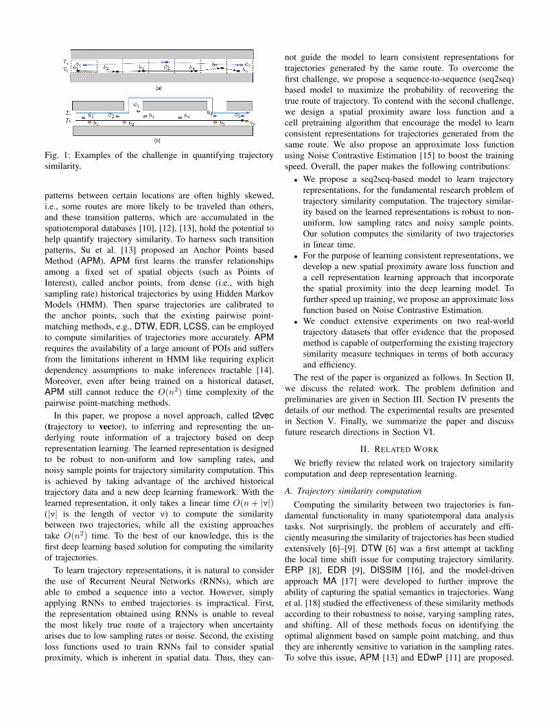
Fig. 1: Examples of the challenge in quantifying trajectorysimilarity.

patterns between certain locations are often highly skewed,i.e., some routes are more likely to be traveled than others,and these transition patterns, which are accumulated in thespatiotemporal databases [10], [12], [13], hold the potential tohelp quantify trajectory similarity. To harness such transitionpatterns, Su et al. [13] proposed an Anchor Points basedMethod (APM). APM first learns the transfer relationshipsamong a fixed set of spatial objects (such as Points ofInterest), called anchor points, from dense (i.e., with highsampling rate) historical trajectories by using Hidden MarkovModels (HMM). Then sparse trajectories are calibrated tothe anchor points, such that the existing pairwise point-matching methods, e.g., DTW, EDR, LCSS, can be employedto compute similarities of trajectories more accurately. APMrequires the availability of a large amount of POIs and suffersfrom the limitations inherent in HMM like requiring explicitdependency assumptions to make inferences tractable [14].Moreover, even after being trained on a historical dataset,APM still cannot reduce the O(n2) time complexity of thepairwise point-matching methods.

In this paper, we propose a novel approach, called t2vec(trajectory to vector), to inferring and representing the un-derlying route information of a trajectory based on deeprepresentation learning. The learned representation is designedto be robust to non-uniform and low sampling rates, andnoisy sample points for trajectory similarity computation. Thisis achieved by taking advantage of the archived historicaltrajectory data and a new deep learning framework. With thelearned representation, it only takes a linear time O(n + |v|)(|v| is the length of vector v) to compute the similaritybetween two trajectories, while all the existing approachestake O(n2) time. To the best of our knowledge, this is thefirst deep learning based solution for computing the similarityof trajectories.

To learn trajectory representations, it is natural to considerthe use of Recurrent Neural Networks (RNNs), which areable to embed a sequence into a vector. However, simplyapplying RNNs to embed trajectories is impractical. First,the representation obtained using RNNs is unable to revealthe most likely true route of a trajectory when uncertaintyarises due to low sampling rates or noise. Second, the existingloss functions used to train RNNs fail to consider spatialproximity, which is inherent in spatial data. Thus, they can-

not guide the model to learn consistent representations fortrajectories generated by the same route. To overcome thefirst challenge, we propose a sequence-to-sequence (seq2seq)based model to maximize the probability of recovering thetrue route of trajectory. To contend with the second challenge,we design a spatial proximity aware loss function and acell pretraining algorithm that encourage the model to learnconsistent representations for trajectories generated from thesame route. We also propose an approximate loss functionusing Noise Contrastive Estimation [15] to boost the trainingspeed. Overall, the paper makes the following contributions:• We propose a seq2seq-based model to learn trajectory

representations, for the fundamental research problem oftrajectory similarity computation. The trajectory similar-ity based on the learned representations is robust to non-uniform, low sampling rates and noisy sample points.Our solution computes the similarity of two trajectoriesin linear time.

• For the purpose of learning consistent representations, wedevelop a new spatial proximity aware loss function anda cell representation learning approach that incorporatethe spatial proximity into the deep learning model. Tofurther speed up training, we propose an approximate lossfunction based on Noise Contrastive Estimation.

• We conduct extensive experiments on two real-worldtrajectory datasets that offer evidence that the proposedmethod is capable of outperforming the existing trajectorysimilarity measure techniques in terms of both accuracyand efficiency.

The rest of the paper is organized as follows. In Section II,we discuss the related work. The problem definition andpreliminaries are given in Section III. Section IV presents thedetails of our method. The experimental results are presentedin Section V. Finally, we summarize the paper and discussfuture research directions in Section VI.

II. RELATED WORK

We briefly review the related work on trajectory similaritycomputation and deep representation learning.

A. Trajectory similarity computation

Computing the similarity between two trajectories is fun-damental functionality in many spatiotemporal data analysistasks. Not surprisingly, the problem of accurately and effi-ciently measuring the similarity of trajectories has been studiedextensively [6]–[9]. DTW [6] was a first attempt at tacklingthe local time shift issue for computing trajectory similarity.ERP [8], EDR [9], DISSIM [16], and the model-drivenapproach MA [17] were developed to further improve theability of capturing the spatial semantics in trajectories. Wanget al. [18] studied the effectiveness of these similarity methodsaccording to their robustness to noise, varying sampling rates,and shifting. All of these methods focus on identifying theoptimal alignment based on sample point matching, and thusthey are inherently sensitive to variation in the sampling rates.To solve this issue, APM [13] and EDwP [11] are proposed.

As discussed in the introduction, APM solves this issue bylearning transition patterns of anchor points from historicaltrajectories. To compute the similarity of two trajectories,EDwP computes the cheapest set of replacement and insertionoperations using linear interpolation to make them identical.Our solution is very different from APM and EDwP in thatwe aim to learn a vector that represents a trajectory andto then compute similarity using the new representation. Inexperiments, we compare with EDwP and not APM for tworeasons: i) The implementation of APM partly requires anabundance of POIs which are not available in our datasets; ii)the more recent EDwP has been reported to perform betterin similarity analysis of trajectories with non-uniform and lowsampling rates. Our work is also related to the inference ofhidden routes from partial observations. Zheng et al. [10] firststudied the problem, and Banerjee et al. [12] further exploredit using Bayesian posterior inference to estimate the top-kmost likely routes. Our work differs from these two in thatour ultimate goal is to learn representations of the trajectoriesrather than solely inferring the most possible routes.

Moreover, all the aforementioned existing measures fortrajectory similarity are based on the dynamic programmingtechnique to identify the optimal alignment which leads toO(n2) computation complexity. Given the complexity, it willbe computationally expensive if we want to apply thesesimilarity measures to cluster a large trajectory database. Incontrast, our method has a linear time complexity O(n+ |v|)to measure the similarity of two trajectories, which is able tosupport analysis on big trajectory data, such as clustering tra-jectories. We can also offer near-instantaneous response timesthat support interactive use, while the competition cannot.

B. Representation learning

Learning representations for specific tasks has been alongstanding open problem in machine learning. Recently,inspired by the success of word2vec [19], the idea of learninggeneral representation has been extended to paragraphs [20],networks [21], [22], etc. To capture the sequential order infor-mation emerging in the sequence processing tasks, RecurrentNeural Networks (RNNs) based encoder-decoder models havebeen developed, such as sequence to sequence learning [23]–[25], and skip-thought vectors [26]. Our model is based onthe general sequence encoder-decoder framework. However,these existing sequence encoder-decoder models were initiallyproposed for natural language processing to deal with discretetokens (i.e., words, punctuations). Our scenarios is different inthat the tokens inherently share the spatial proximity relation.Our model therefore differs from the above sequence encoder-decoders in two ways: i) we design a spatial proximity awareloss function and a cell representation pretraining approach toincorporate the spatial proximity into the deep representationmodel, and ii) we also propose an approximate loss functionbased on Noise Contrastive Estimation to accelerate the train-ing.

III. DEFINITIONS AND PRELIMINARIES

In this section, we present definitions and preliminariesessential to understand the problem addressed and the se-quence encoder-decoder model used in our solution. For easeof reference, frequently used notation is given in Table I.

TABLE I: Frequently used notation.

Symbol DefinitionT (or Ta) TrajectoryR Underlying routex A sequence of tokensxt Token at position tx1:t A sequence of tokens from position 1 to t|T | (or |x|) Length of T (or x)v Embedded vectorht Hidden state (vector)V Vocabularyr1 (r2) Dropping rate (distorting rate)

A. Definitions

We next define the notions of underlying route and trajec-tory.

Definition 1. (UNDERLYING ROUTE) An underlying routeof a moving object is a continuous spatial curve (e.g., in thelongitude-latitude domain), indicating the exact path taken bythe object.

The underlying route is only a theoretical concept as lo-cation acquisition techniques do not record moving locationscontinuously.

Definition 2. (TRAJECTORY) A trajectory T is a sequence ofsample points from the underlying route of a moving object.

In practice, an underlying route can be represented by enor-mous trajectories, depending on the specifics of the movingobjects and the sampling strategies used. Each generated tra-jectory can be considered as a representative of an underlyingroute. In the rest of this paper, a trajectory is also referred toas trip, depending on the context.Problem statement. Given a collection of historical trajec-tories, we aim to learn a representation v ∈ Rn (n is thedimension of a Euclidean space) for each trajectory T suchthat the representation can reflect the underlying route of thetrajectory for computing trajectory similarity. The similarity oftwo trajectories based on the learned representations must berobust to non-uniform, low sampling rates and noisy samplepoints.

Our proposed method for solving the problem is based ondeep representation learning techniques. Specifically, we adaptthe sequence encoder-decoder framework for the first time tocompute trajectory similarity (the motivation for adapting thatparticular framework is explained in Section IV-A).

B. Preliminaries of sequence encoder-decoders

We briefly present the sequence encoder-decoder frame-work. Consider two sequences x = 〈xt〉|x|t=1 and y = 〈yt〉|y|t=1

where each xt and yt denotes token (e.g., a word or punc-tuation mark in a natural language sentence) and |x| and|y| represent lengths. We next illustrate how to build theconditional probability P(y|x) in the framework.

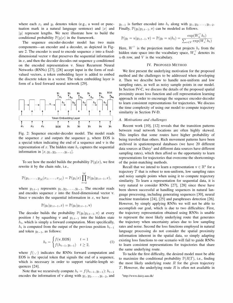
The sequence encoder-decoder model has two maincomponents—an encoder and a decoder, as depicted in Fig-ure 2. The encoder is used to encode sequence x into a fixed-dimensional vector v that preserves the sequential informationin x, and then the decoder decodes out sequence y conditionedon the encoded representation v. Since Recurrent NeuralNetworks (RNNs) [27], [28] accept input in the form of real-valued vectors, a token embedding layer is added to embedthe discrete token in a vector. The token embedding layer isform of a feed forward neural network [29].

Fig. 2: Sequence encoder-decoder model. The model readsthe sequence x and outputs the sequence y, where EOS isa special token indicating the end of a sequence and v is therepresentation of x. The hidden state ht captures the sequentialinformation in [x, y1, y2, . . . , yt−1].

To see how the model builds the probability P(y|x), we firstrewrite it by the chain rule, i.e.,

P(y1, . . . , y|y||x1, . . . , x|x|) = P(y1|x)|y|∏t=2

P(yt|y1:t−1, x),

where y1:t−1 represents y1, y2, . . . , yt−1. The encoder readsand encodes sequence x into the fixed-dimensional vector v.Since v encodes the sequential information in x, we have

P(yt|y1:t−1, x) = P(yt|y1:t−1, v)

The decoder builds the probability P(yt|y1:t−1, v) at everyposition t by squashing v and y1:t−1 into the hidden stateht, which is simply a forward computation. More specifically,ht is computed from the output of the previous position ht−1and token yt−1, as follows:

ht =

{f(v,EOS) t = 1

f(ht−1, yt−1) t ≥ 2,(1)

where f(·, ·) indicates the RNNs forward computation andEOS is the special token that signals the end of a sequence,which is necessary in order to support variable-length se-quences [24].

Note that we recursively compute ht = f(ht−1, yt−1): ht−1encodes the information of v along with y1, y2, . . . , yt−2, and

yt−1 is further encoded into ht along with y1, y2, . . . , yt−2.Finally, P(yt|y1:t−1, v) can be modeled as follows.

P(yt = u|y1:t−1, v) = P(yt = u|ht) =exp(W>u ht)∑

v∈V exp(W>v ht)

Here, W> is the projection matrix that projects ht from thehidden state space into the vocabulary space, W>u denotes itsu-th row, and V is the vocabulary.

IV. PROPOSED METHOD

We first present the underlying motivation for the proposedmethod and the challenges to be addressed when developingit. Then we describe how to handle non-uniform and lowsampling rates, as well as noisy sample points in our model.In Section IV-C, we discuss the details of the proposed spatialproximity aware loss function and cell representation learningapproach in order to encourage the sequence encoder-decoderto learn consistent representations for trajectories. We discussthe time complexity of using our model to compute trajectorysimilarity in Section IV-D.

A. Motivations and challenges

Recent work [10], [12] reveals that the transition patternsbetween road network locations are often highly skewed.This implies that some routes have higher probability ofbeing traveled than others. Rich movement patterns have beenarchived in spatiotemporal databases (we have 20 differentdata sources at Daisy1 and different data sources have differentsampling rates), which then afford us the opportunity to learnrepresentations for trajectories that overcome the shortcomingsof the point-matching methods.

Recall that we intend to learn a representation v ∈ Rn for atrajectory T that is robust to non-uniform, low sampling ratesand noisy sample points when using it to compute trajectorysimilarity. To learn a representation for sequential data, it isvery natural to consider RNNs [27], [28] since these havebeen shown successful at handling sequences in natural lan-guage processing, including generating sequences [30], neuralmachine translation [24], [25] and paraphrases detection [26].However, by simply applying RNNs we will not be able toaccomplish our goal, which is due to two difficulties: First,the trajectory representation obtained using RNNs is unableto represent the most likely underlying route that generatesthe trajectory when uncertainty arises due to low samplingrates and noise. Second the loss functions employed in naturallanguage processing do not consider the spatial proximityinformation inherent in the spatial data, so simply adaptingexisting loss functions to our scenario will fail to guide RNNsto learn consistent representations for trajectories that sharethe same underlying route.

To tackle the first difficulty, the desired model must be ableto maximize the conditional probability P(R|T ), i.e., findingthe most likely underlying route R for the given trajectoryT . However, the underlying route R is often not available in

1http://www.daisy.aau.dk/

practice. To circumvent this, we exploit two observations: i)both a non-uniform, relatively low sampling rate trajectory,denoted by Ta, and a relatively high sampling rate trajectory,denoted by Tb, are paraphrases of their underlying route,and ii) a relatively high sampling rate trajectory Tb is closerto their true underlying route R than is Ta, and it haslower uncertainty. These observations cause us to replacethe objective of maximizing P(R|Ta) into the objective ofmaximizing P(Tb|Ta) and to build the model using a sequenceencoder-decoder framework. The encoder embeds Ta intoits representation v, and the decoder will try to recover itscounterpart Tb with relatively high sampling rate conditionedon v by optimizing its parameters. When the model is trainedusing the real-world trajectories, the transition patterns hiddenin historical data will be learned by the model. To overcomethe second difficulty, we propose a new spatial proximityaware loss function and cell (token) representation pre-trainingmethod to incorporate spatial proximity into the model. Toaccelerate the training, we develop an approximate spatialproximity aware loss function based on Noise ContrastiveEstimation [15].

B. Handling varying sampling rates and noise

Based on the above analysis, given a collection of samplingrate trajectories {T (i)

b }Ni=1 (where N is the cardinality of thecollection), we create a collection of pairs (Ta, Tb), where Tb isan original trajectory and Ta is obtained by randomly droppingsample points from Tb with dropping rate r1. By doing so,each down-sampled Ta is also non-uniformly sampled andthus represents a real-life trajectory with non-uniform and lowsampling rate. The start and end points of Tb are preservedin Ta to avoid changing the underlying route of the down-sampled trajectory. To illustrate, consider generating the sub-trajectories for Tb in Figure 1b, we randomly drop points inb2:5, i.e., all generated sub-trajectories will start with b1 andend with b6. After the generating procedure, we maximizethe joint probability of all (Ta, Tb) pairs with the sequenceencoder-decoder model:

maximizeN∏i=1

P(T (i)b |T

(i)a ) (2)

In the sequence encoder-decoder model, the inputs shouldbe sequences of discrete tokens. Therefore, we need to finda way to map the continuous coordinates (i.e., longitude,latitude) into discrete tokens (analogous to words in naturallanguage). We adopt a simple strategy that is used commonlyin spatial data analytics, i.e., we partition the space into cellsof equal size [31] and treat each cell as a token. All samplepoints falling into the same cell are then mapped to the sametoken.

The above helps mainly to overcome the problems of non-uniform and low sampling rates. However, the realistic trajec-tories also may have noisy sample points. For example, whena GPS receiver is in an urban canyon and satellite visibilityis poor, inaccurate locations may result. To eliminate the

influence of noisy sample points, we only keep the cells whichare hit by more than δ sample points. These cells are referredto as hot cells and form the final vocabulary V (in the rest ofpaper, we will interchangeably use token and cell to refer toan element V ). Sample points are represented by their nearesthot cell. To make the learned representations more robust tothe noisy data, we further distort each downsampled Ta basedon a distorting rate r2 to create the distorted variants, i.e., werandomly sample a fraction of the points (size indicated by r2)that are then distorted. Point (px, py) is distorted by adding aGaussian noise with a radius 30 (meters) as follows,

px = px + 30 · dx, dx ∼ Gaussian(0, 1)py = py + 30 · dy, dy ∼ Gaussian(0, 1)

(3)

We can optimize the same objective as shown in Equation 2where Ta is both downsampled and distorted.

C. Learning consistent representations

The original sequence encoder-decoder does not model thespatial correlation between cells, which is important in orderto learn consistent representations for trajectories drawn fromthe same route. To address this, we propose a novel spatialproximity aware loss function (in Section IV-C1) and a newcell representation pretraining approach that takes into accountspatial proximity (in Section IV-C2) To further improve thetraining, an approximate loss function based on Noise Con-trastive Estimation [15] is also proposed (in Section IV-C1).

1) Spatial proximity aware loss function: To train a se-quence encoder-decoder, we need a loss function to character-ize the optimization objective. This is important, as differencesin the loss function would encourage the model to learndifferent representations [32]. When the sequence encoder-decoder is employed in natural language processing, e.g.,in neural machine translation [23], [24], [33], Negative LogLikelihood (NLL) loss is chosen to minimize the negative loglikelihood function for tokens in the target sentence as follows,

L1 = − log∏t

P(yt|y1:t−1, x) (4)

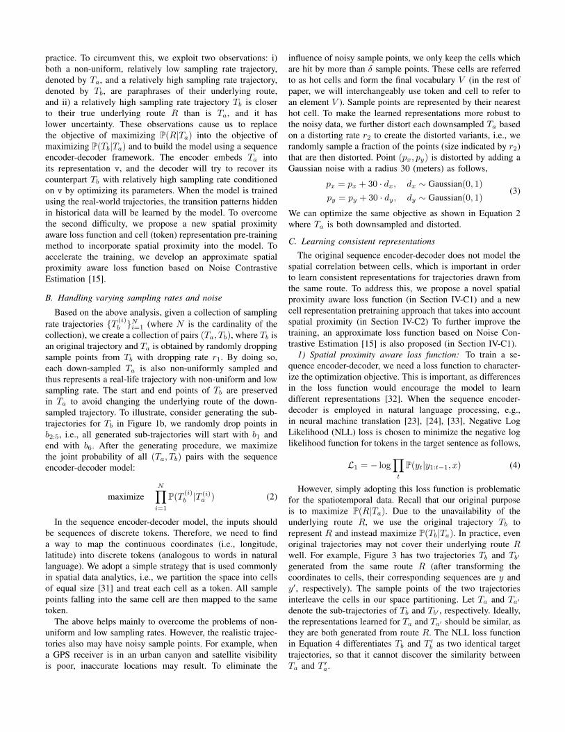
However, simply adopting this loss function is problematicfor the spatiotemporal data. Recall that our original purposeis to maximize P(R|Ta). Due to the unavailability of theunderlying route R, we use the original trajectory Tb torepresent R and instead maximize P(Tb|Ta). In practice, evenoriginal trajectories may not cover their underlying route Rwell. For example, Figure 3 has two trajectories Tb and Tb′

generated from the same route R (after transforming thecoordinates to cells, their corresponding sequences are y andy′, respectively). The sample points of the two trajectoriesinterleave the cells in our space partitioning. Let Ta and Ta′

denote the sub-trajectories of Tb and Tb′ , respectively. Ideally,the representations learned for Ta and Ta′ should be similar, asthey are both generated from route R. The NLL loss functionin Equation 4 differentiates Tb and T ′b as two identical targettrajectories, so that it cannot discover the similarity betweenTa and T ′a.

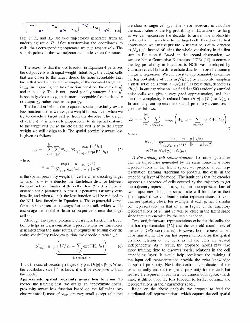
Fig. 3: Tb and Tb′ are two trajectories generated from anunderlying route R. After transforming the coordinates tocells, their corresponding sequences are y, y′ respectively. Thesample points in the two trajectories interleave on the route.

The reason is that the loss function in Equation 4 penalizesthe output cells with equal weight. Intuitively, the output cellsthat are closer to the target should be more acceptable thanthose that are far way. For example, if the decoded target cellis y3 (in Figure 3), the loss function penalizes the outputs y′3and y1 equally. This is not a good penalty strategy. Since y′3is spatially closer to y3, it is more acceptable for the decoderto output y′3 rather than to output y1.

The intuition behind the proposed spatial proximity awareloss function is that we assign a weight for each cell when wetry to decode a target cell yt from the decoder. The weightof cell u ∈ V is inversely proportional to its spatial distanceto the target cell yt, so the closer the cell is to yt the largerweight we will assign to it. The spatial proximity aware lossis given as follows.

L2 = −|y|∑t=1

∑u∈V

wuyt logexp(W>u ht)∑

v∈V exp(W>v ht), (5)

where

wuyt =exp (−||u− yt||2/θ)∑v∈V exp(−||v − yt||2/θ)

is the spatial proximity weight for cell u when decoding targetyt, and ||u − yt||2 denotes the Euclidean distance betweenthe centroid coordinates of the cells. Here θ > 0 is a spatialdistance scale parameter. A small θ penalizes far away cellsheavily, and when θ → 0, the loss function will be reduced tothe NLL loss function in Equation 4. The exponential kernelfunction is chosen as it decays fast at the tail, which wouldencourage the model to learn to output cells near the targetcell yt.

Although the spatial proximity aware loss function in Equa-tion 5 helps us learn consistent representations for trajectoriesgenerated from the same routes, it requires us to sum over theentire vocabulary twice every time we decode a target yt:∑

u∈V wuyt

(W>u ht −

∑v∈V

exp(W>v ht)

)︸︷︷︸

log probability

(6)

Thus, the cost of decoding a trajectory y is O(|y|×|V |). Whenthe vocabulary size |V | is large, it will be expensive to trainthe model.Approximate spatial proximity aware loss function. Toreduce the training cost, we design an approximate spatialproximity aware loss function based on the following twoobservations: i) most of wuyt

are very small except cells that

are close to target cell yt; ii) it is not necessary to calculatethe exact value of the log probability in Equation 6, as longas we can encourage the decoder to assign the probabilityto the cells that are close to the target cell. Based on the firstobservation, we can use just the K nearest cells of yt, denotedas NK(yt), instead of using the whole vocabulary in the firstsum in Equation 6. Based on the second observation, wecan use Noise Contrastive Estimation (NCE) [15] to computethe log probability in Equation 6. NCE was developed byGutmann et al. [15] to differentiate data from noise by traininga logistic regression. We can use it to approximately maximizethe log probability of cells in NK(yt) by randomly samplinga small set of cells from V −NK(yt) as noise data, denoted asO(yt). In our experiments, we find that 500 randomly samplednoise cells can give a very good approximation, and thusthe time complexity is reduced from O(|y| × |V |) to O(|y|).In summary, our approximate spatial proximity aware loss isgiven as follows.

L3 = −|y|∑t=1

∑u∈NK(yt)

wuyt

(W>u ht −

∑v∈NO

exp(W>v ht)

),

(7)where

wuyt =exp (−||u− yt||2/θ)∑

v∈NK(yt)exp(−||v − yt||2/θ)

NO = NK(yt) ∪ O(yt)2) Pre-training cell representations: To further guarantee

that the trajectories generated by the same route have closerepresentations in the latent space, we propose a cell rep-resentation learning algorithm to pre-train the cells in theembedding layer of the model. The intuition is that the encodersqueezes a sequence of cells covered by the trajectory to getthe trajectory representation v, and thus the representations oftwo trajectories along the same route will be close in theirlatent space if we can learn similar representations for cellsthat are spatially close. For example, if each yi has a similarcell representation as that of y′i in Figure 3, the trajectoryrepresentations of Ta and T ′a will be close in the latent spacesince they are encoded by the same encoder.

Two straightforward representations exist for the cells, theone-hot representation [32] and the centroid coordinates ofthe cells (GPS coordinates). However, both representationshave limitations. The one-hot representation loses the spatialdistance relation of the cells as all the cells are treatedindependently. As a result, the proposed model may takemore training time to discover spatial relations in the cellembedding layer. It would help accelerate the training ifthe input cell representations provide the prior knowledgeof spatial proximity. Next, the centroid coordinates of thecells naturally encode the spatial proximity for the cells butrestrict the representations in a two-dimensional space, whichmake it difficult for the loss function to further optimize therepresentations in their parameter space.

Based on the above analysis, we propose to feed thedistributed cell representations, which capture the cell spatial

proximity relation, to the embedding layer of the model. Weachieve this by borrowing the key idea from skip-grams [19].The intuition behind skip-grams is that words with similarmeanings tend to appear together in the same contexts, and ifwe use the representation of a word to predict its surroundingwords then we can embed the words into a Euclidean space ina way that captures the semantic distances between the words.Towards this end, we create the context for a given cell u ∈ Vby randomly sampling its neighbor u′ ∈ NK(u) (we also onlyconsider its K-nearest neighbors) according to the followingcell sampling distribution:

P(u′) =exp(−||u′ − u||2/θ)∑

v∈NK(u) exp(−||v − u||2/θ)(8)

The cell sampling distribution is similar to the spatial proxim-ity weight in Equation 5. Note that their θ values do not have tobe equal. For each cell u ∈ V , the cell sampling distributiontends to sample the cells that are spatially close to it as itscontext. In this fashion, we are able to create the context foreach cell and to learn the cell representation efficiently withthe negative sampling algorithm [34] by maximizing the logprobability of observing the neighboring cells in its context,C(u), given cell u:

maximize∑u∈V

logP(C(u)|g(u)) (9)

Here, g(u) denotes the representation of cell u. The learnedcell representations will be used to initialize the embeddinglayer in the model, but we do not fix their values. Thusthey can still be further optimized by the loss function inEquation 7. The learning algorithm is shown in Algorithm 1.

Algorithm 1: CellLearning (CL)Input: The dimension of the learned representations d, context window

size lOutput: The learned cell representations g(u)

1 for u ∈ V do2 C(u)← ∅ ;3 while |C(u)| < l do4 u′ ∼ P(u′) according to Equation 8;5 C(u)← C(u) ∪ u′;

6 Optimizing the loss function in Equation 9;7 return g(u) for u ∈ V ;

D. Complexity of similarity computation

Our model can be trained completely unsupervised with theSGD (Stochastic Gradient Descent) algorithm. Given a trainedmodel, it only requires O(n) time (as shown in Equation 1,where f(·, ·) indicates the encoder-RNN and h0 is a zerovector) to embed a trajectory into a vector which is fast andcan be done using GPUs. Then we can use the Euclideandistance of the two vectors to measure the similarity of twotrajectories, with a time complexity of O(|v|). Therefore thetime complexity of measuring the similarity between twotrajectories is O(n+ |v|).

TABLE II: Dataset statistics.

Dataset #Points #Trips Mean lengthPorto 74,269,739 1,233,766 60

Harbin 184,809,109 1,527,348 121

V. EXPERIMENTS

We study the effectiveness and scalability of our proposedmethod on two real-world taxi datasets. The experimentalsetup and parameter settings are presented in Sections V-Aand V-B respectively. Then we evaluate the accuracy of differ-ent methods using most similar search, cross-similarity, and k-nn queries in Sections V-C1 to V-C3, respectively. Scalabilityis covered in Section V-D. The proposed loss functions andcell learning approach are evaluated in Section V-E. We end byevaluating the impact of the cell size, the hidden state size ofthe encoder, and the training data size on the learned trajectoryrepresentations in Sections V-F and V-G.

A. Experimental setup

Dataset. The experiments are conducted on two real-worldtaxi datasets. The first dataset2 is collected in the city of Porto,Portugal over 19 months and contains 1.7 million trajectories.Each taxi reports its location at 15 second intervals. We removetrajectories with length less than 30, which yields 1.2 milliontrajectories. The second dataset contains trajectories collectedfrom 13,000 taxis over 8 months in Harbin, China. We selecttrajectories with length at least 30 and time gaps between con-secutive sample points being less than 20 second. This yields1.5 million trajectories. We partition both sets into trainingdata and testing data based on the starting timestamp of thetrajectories. For both sets, the first 0.8 million trajectories areused for training, and the remaining trajectories are used fortesting. Statistics of the two sets are shown in Table II.

To create the training trajectory pairs as described in Sec-tion IV-A, we perform two kinds of transformations, down-sampling and distortion. For each trajectory Tb we first down-sample it with a dropping rate r1 varied in [0, 0.2, 0.4, 0.6]to create its 4 sub-trajectories Ta. And we further distort eachdown-sampled Ta based on a distorting rate r2 (as described inEquation 3) varied in [0, 0.2, 0.4, 0.6]. As a result, 16 trainingpairs (Ta, Tb) are created for each original trajectory Tb.Benchmarking Methods: We compare t2vec with threeother methods for measuring the trajectory similarity, namelyEDR [9], LCSS [7], and EDwP [11]. LCSS and EDR aretwo of the most widely adopted trajectory similarity measuresin spatiotemporal data analyses. EDwP is the state-of-the-artmethod for measuring similarity of non-uniform and low sam-pling rate trajectories. We do not include DTW as it has beendemonstrated to be consistently inferior to EDR in trajectorysimilarity computation [11]. Moreover, we compare with thevanilla RNN (vRNN) [35] and the common set representation(CMS). The vanilla RNN serves as an embedding baselinemethod, and the common set representation is used to measure

2http://www.geolink.pt/ecmlpkdd2015-challenge

the similarity of two trajectories based on their common setafter they have been mapped to cells. We discuss the reasonsfor comparing with the two baselines in Section V-C1.Evaluation Platform: Our method3 is implemented in Ju-lia [36] and PyTorch, and trained using a Tesla K40 GPU.The baseline methods are written in Java4. The platform runsthe Ubuntu 14.04 operating system with an Intel Xeon E5-1620 CPU.

B. Parameter settings and training details

Cell size: The default cell size in the experiments is 100meters. After removing the cells hit by less than 50 points(i.e., δ = 50), we get 18,866 hot cells for the Porto datasetand 22,171 hot cells for the Harbin dataset.RNN units: In our model, GRU [35] with 3 layers is chosenas the computational unit because it has been shown to be asgood as LSTM [37] in sequence modeling tasks, while it ismuch more efficient to compute [35].Gradient clipping: Although RNNs tend not suffer fromgradient vanishing problem, they may have exploding gra-dients [38]. Hence, we clip the gradients by enforcing amaximum gradient norm constraint [30], which is set to 5in our experiments.Terminating condition: We randomly select 10,000 trajecto-ries as a validation dataset from the test dataset (the selectedtrajectories are removed from the test dataset). The trainingis terminated if the loss in the validation dataset does notdecrease in 20,000 successive iterations.

In addition, both the hidden layer size in GRU and thedimension of the learned cell representation d are set to 256,the context window size l in the cell learning algorithm is setto 10. For simplicity, θ in Equations 5 and 8 is fixed at 100(meters). Parameter K and the size of O(yt) in Section IV-Care set to 20 and 500, respectively. We adopt Adam stochasticgradient descent [39] with an initial learning rate of 0.001 totrain the model. We evaluate the training time in Sections V-Eand V-F.

To set the parameter ε of the baseline methods EDR andLCSS, we adopt the strategies described in the studies [7], [9]proposing the two methods; the parameters of vRNN are setto be the same as our encoder-RNN except that it is trained bypredicting the next cell based on the cells that it has alreadyseen.

C. Performance evaluation

The lack of ground-truth dataset makes it a challengingproblem to evaluate the accuracy of trajectory similarity. Tworecent studies [11], [13] propose to evaluate the accuracy ofmethods for computing trajectory similarity using the self-similarity and cross-similarity comparisons and assessmentsof the precision of finding the k-nearest neighbors. Currently,this is the best evaluation methodology, and we adopt thismethodology in the experiments. In addition, we also designa new experiment, called most similar search (which can be

3https://github.com/boathit/research-papers/tree/master/t2vec4The authors of EDwP give us access to their compiled jar file.

TABLE III: Mean rank versus the database size using the Portoand Harbin datasets.

PortoDB size 20k 40k 60k 80k 100k

EDR 25.73 50.70 76.07 104.01 130.98LCSS 31.95 59.20 95.85 130.40 150.67CMS 62.18 112.84 173.34 231.55 291.26vRNN 32.73 61.24 100.20 135.22 163.10EDwP 6.78 11.48 16.08 23.02 28.90t2vec 2.30 3.45 4.73 6.35 7.67

HarbinDB size 20k 40k 60k 80k 100k


considered as a sort of self-similarity measure) to evaluate theeffectiveness of different methods, in Section V-C1.

One of the most important tasks in trajectory analysis issimilar trajectory search. To overcome the lack of ground-truth, we design three experiments to evaluate the performanceusing different methods for this task.

We randomly choose 10,000 trajectories from the testdataset, denoted as Q, and then we choose another m (aparameter to be evaluated) trajectories, denoted by P . Foreach trajectory Tb ∈ Q, we create two sub-trajectories fromit by alternately taking points from it, denoted as Ta and Ta′

(see Figure 4), and we use them to construct two datasetsDQ = {Ta} and D′Q = {Ta′}. We perform the sametransformation for the trajectories in P to get DP and D′P .Then for each query Ta ∈ DQ, we retrieve its top-k mostsimilar trajectories from database D′Q ∪D′P and calculate therank of Ta′ . Ideally Ta′ is ranked at the top since it is generatedfrom the same original trajectory as Ta. The reason for usingD′Q ∪D′P as the database instead of D′Q ∪P is that the querytrajectory will have similar mean length as the trajectories inthe database5. Moreover, to evaluate whether RNN encodestwo sequences of cells into two similar vectors simply becausethe two sequences have the same starting or ending cells, orjust because they have sufficient numbers of common cells,we include another two baselines, vRNN and CMS. If theaforementioned reason is true, vRNN and CMS should alsogive good performance in the task.

Fig. 4: Creating two sub-trajectories Ta and Ta′ from trajectoryTb by alternately taking points from it.

1) Most similar trajectory search: Experiment 1 We firststudy the performance of the different methods when weincrease m, the size of P , from 20,000 to 100,000. Table III

5Similar results were found using database D′Q ∪ P .

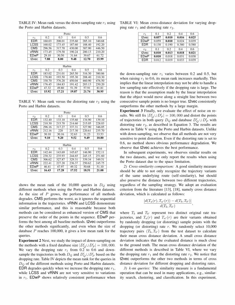
TABLE IV: Mean rank versus the down-sampling rate r1 usingthe Porto and Harbin datasets.

Portor1 0.2 0.3 0.4 0.5 0.6


Harbinr1 0.2 0.3 0.4 0.5 0.6


TABLE V: Mean rank versus the distorting rate r2 using thePorto and Harbin datasets.

Portor2 0.2 0.3 0.4 0.5 0.6

EDR 132.40 133.10 135.60 134.90 139.10LCSS 210.30 215.70 214.60 215.05 228.03CMS 296.16 317.27 337.31 327.90 346.05vRNN 212.16 220 217.30 220.61 235.70EDwP 30.10 30.16 32.63 31.23 33.53t2vec 9.10 9.20 9.52 9.49 10.80

Harbinr2 0.2 0.3 0.4 0.5 0.6


shows the mean rank of the 10,000 queries in DQ usingdifferent methods when using the Porto and Harbin datasets.As the size of P grows, the performance of all methodsdegrades. CMS performs the worst, as it ignores the sequentialinformation in the trajectories. vRNN and LCSS demonstratesimilar performance, and this is reasonable because bothmethods can be considered as enhanced version of CMS thatpreserve the order of the points in the sequence. EDwP per-forms the best among all baseline methods. t2vec outperformsthe other methods significantly, and even when the size ofdatabase P reaches 100,000, it gives a low mean rank for thequeries.Experiment 2 Next, we study the impact of down-sampling onthe methods with a fixed database size |D′Q∪D′P | = 100, 000.We vary the dropping rate r1 from 0.2 to 0.6 and down-sample the trajectories in both DQ and D′Q∪D′P based on thedropping rate. Table IV depicts the mean rank for the queries inDQ of the different methods using Porto and Harbin datasets.EDR degrades quickly when we increase the dropping rate r1,while LCSS and vRNN are not very sensitive to variationsin r1. EDwP shows relatively consistent performance when

TABLE VI: Mean cross-distance deviation for varying drop-ping rate r1 and distorting rate r2.

r1 0.1 0.2 0.4 0.6t2vec 0.057 0.010 0.016 0.025EDwP 0.059 0.010 0.024 0.039EDR 0.130 0.190 0.380 0.580r2 0.1 0.2 0.4 0.6

t2vec 0.010 0.013 0.018 0.021EDwP 0.010 0.018 0.031 0.038EDR 0.012 0.019 0.033 0.039

the down-sampling rate r1 varies between 0.2 and 0.5, butwhen raising r1 to 0.6, its mean rank increases markedly. Thisimplies that the linear interpolation may not be able to handle alow sampling rate effectively if the dropping rate is large. Thereason is that the assumption made by the linear interpolationthat the object would move along a straight line between twoconsecutive sample points is no longer true. t2vec consistentlyoutperforms the other methods by a large margin.Experiment 3 Finally, we evaluate the effect of noise on re-sults. We still fix |D′Q∪D′P | = 100, 000 and distort the pointsof trajectories in both query DQ and database D′Q ∪D′P withdistorting rate r2, as described in Equation 3. The results areshown in Table V using the Porto and Harbin datasets. Unlikewith down-sampling, we observe that all methods are not verysensitive to point distortion. Even if the distorting rate is set to0.6, no method shows obvious performance degradation. Weobserve that t2vec achieves the best performance.

In subsequent experiments, we observes similar results onthe two datasets, and we only report the results when usingthe Porto dataset due to the space limitation.

2) Cross-similarity comparison: A good similarity measureshould be able to not only recognize the trajectory variantsof the same underlying route (self-similarity), but shouldalso preserve the distance between two different trajectories,regardless of the sampling strategy. We adopt an evaluationcriterion from the literature [13], [18], namely cross distancedeviation, which is calculated as follows:

|d(Ta(r), Ta′(r))− d(Tb, Tb′)|d(Tb, Tb′)

,

where Tb and Tb′ represent two distinct original rate tra-jectories, and Ta(r) and Ta′(r) are their variants obtainedby randomly dropping (or distorting) sample points with thedropping (or distorting) rate r. We randomly select 10,000trajectory pairs (Tb, Tb′) from the test dataset to calculatetheir mean cross distance deviation. A small cross distancedeviation indicates that the evaluated distance is much closeto the ground truth. The mean cross distance deviation of thedifferent methods is described in Table VI, where we varythe dropping rate r1 and the distorting rate r2. We notice thatt2vec outperforms the other two methods in terms of crossdistance deviation for different dropping and distorting rates.

3) k-nn queries: The similarity measure is a fundamentaloperation that can be used in many applications, e.g., similar-ity search, clustering, and classification. In this experiment,

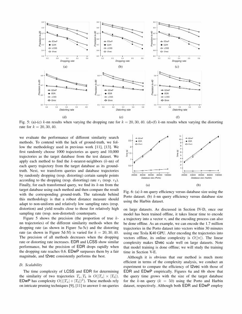
(a) (b) (c)

(d) (e) (f)Fig. 5: (a)-(c) k-nn results when varying the dropping rate for k = 20, 30, 40. (d)-(f) k-nn results when varying the distortingrate for k = 20, 30, 40.

we evaluate the performance of different similarity searchmethods. To contend with the lack of ground-truth, we fol-low the methodology used in previous work [11], [13]. Wefirst randomly choose 1000 trajectories as query and 10,000trajectories as the target database from the test dataset. Weapply each method to find the k-nearest-neighbors (k-nn) ofeach query trajectory from the target database as its ground-truth. Next, we transform queries and database trajectoriesby randomly dropping (resp. distorting) certain sample pointsaccording to the dropping (resp. distorting) rate r1 (resp. r2).Finally, for each transformed query, we find its k-nn from thetarget database using each method and then compare the resultwith the corresponding ground-truth. The rationale behindthis methodology is that a robust distance measure shouldadapt to non-uniform and relatively low sampling rates (resp.distortion) and yield results close to those for relatively highsampling rate (resp. non-distorted) counterparts.

Figure 5 shows the precision (the proportion of true k-nn trajectories) of the different similarity methods when thedropping rate (as shown in Figure 5a-5c) and the distortingrate (as shown in Figure 5d-5f) is varied for k = 20, 30, 40.The precision of all methods decreases when the droppingrate or distorting rate increases. EDR and LCSS show similarperformance, but the precision of EDR drops rapidly whenthe dropping rate reaches 0.6. EDwP surpasses them by a fairmagnitude, and t2vec consistently performs the best.

D. Scalability

The time complexity of LCSS and EDR for determiningthe similarity of two trajectories Ta, Tb is O(|Ta| × |Tb|).EDwP has complexity O((|Ta|+ |Tb|)2). These methods relyon intricate pruning techniques [9], [11] to answer k-nn queries

(a) (b)

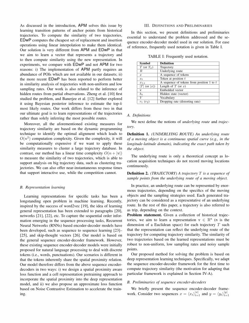
Fig. 6: (a) k-nn query efficiency versus database size using thePorto dataset. (b) k-nn query efficiency versus database sizeusing the Harbin dataset.

on large datasets. As discussed in Section IV-D, once ourmodel has been trained offline, it takes linear time to encodea trajectory into a vector v, and the encoding process can alsobe done offline. As an example, we can encode the 1.7 milliontrajectories in the Porto dataset into vectors within 30 minutesusing one Tesla K40 GPU. After encoding the trajectories intovectors offline, its online complexity is O(|v|). The linearcomplexity makes t2vec scale well on large datasets. Notethat model training is done offline; we will study the trainingtime in Section V-E.

Although it is obvious that our method is much moreefficient in terms of the complexity analysis, we conduct anexperiment to compare the efficiency of t2vec with those ofEDR and EDwP empirically. Figures 6a and 6b show thatthe query time grows with the size of the target databasefor the k-nn query (k = 50) using the Porto and Harbindataset, respectively. Although both EDR and EDwP employ

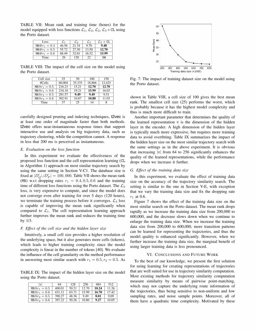
TABLE VII: Mean rank and training time (hours) for themodel equipped with loss functions L1, L2, L3, L3+CL usingthe Porto dataset.

Loss L1 L2 L3 L3 + CL

MR@r1 = 0.4 46.56 21.34 9.70 9.48MR@r1 = 0.5 55.72 27.30 13.50 12.70MR@r1 = 0.6 68.49 32.01 16.52 15.99

Time 26 120 22 14

TABLE VIII: The impact of the cell size on the model usingthe Porto dataset.

Cell size 25 50 100 150#Cells 60,004 35,335 18,866 12,425

MR@r1 = 0.5 216.23 15.21 12.70 12.70MR@r1 = 0.6 234.18 19.21 15.99 16.03MR@r2 = 0.5 291.57 9.49 9.49 9.51MR@r2 = 0.6 302.91 10.87 10.80 11.03

Time 37 25 14 8

carefully designed pruning and indexing techniques, t2vec isat least one order of magnitude faster than both methods.t2vec offers near-instantaneous response times that supportinteractive use and analysis on big trajectory data, such astrajectory clustering, while the competition cannot. A responsein less that 200 ms is perceived as instantaneous.

E. Evaluation on the loss function

In this experiment we evaluate the effectiveness of theproposed loss function and the cell representation learning (CLin Algorithm 1) approach on most similar trajectory search byusing the same setting in Section V-C1. The database size isfixed at |D′Q∪D′P | = 100, 000. Table VII shows the mean rank(MR) w.r.t dropping rates r1 = 0.4, 0.5, 0.6 and the trainingtime of different loss functions using the Porto dataset. The L2

loss, is very expensive to compute, and since the model doesnot converge even after training for over 5 days (120 hours),we terminate the training process before it converges. L3 lossis capable of improving the mean rank significantly whencompared to L1. The cell representation learning approachfurther improves the mean rank and reduces the training timeby 1/3.

F. Effect of the cell size and the hidden layer size

Intuitively, a small cell size provides a higher resolution ofthe underlying space, but it also generates more cells (tokens),which leads to higher training complexity since the modelcomplexity is linear in the number of tokens [40]. We evaluatethe influence of the cell granularity on the method performancein answering most similar search with r1 = 0.5, r2 = 0.5. As

TABLE IX: The impact of the hidden layer size on the modelusing the Porto dataset.

|v| 64 128 256 484 512MR@r1 = 0.5 400.01 50.21 12.70 10.24 11.26MR@r1 = 0.6 431.11 63.71 15.99 16.70 17.42MR@r2 = 0.5 390.27 48.36 9.49 8.01 9.09MR@r2 = 0.6 397.22 50.26 10.80 9.27 10.05

Fig. 7: The impact of training dataset size on the model usingthe Porto dataset.

shown in Table VIII, a cell size of 100 gives the best meanrank. The smallest cell size (25) performs the worst, whichis probably because it has the highest model complexity andthus is much more difficult to train.

Another important parameter that determines the quality ofthe learned representation v is the dimension of the hiddenlayer in the encoder. A high dimension of the hidden layeris typically much more expressive, but requires more trainingdata to avoid overfitting. Table IX summarizes the impact ofthe hidden layer size on the most similar trajectory search withthe same settings as in the above experiment. It is obviousthat increasing |v| from 64 to 256 significantly enhances thequality of the learned representations, while the performancedrops when we increase it further.

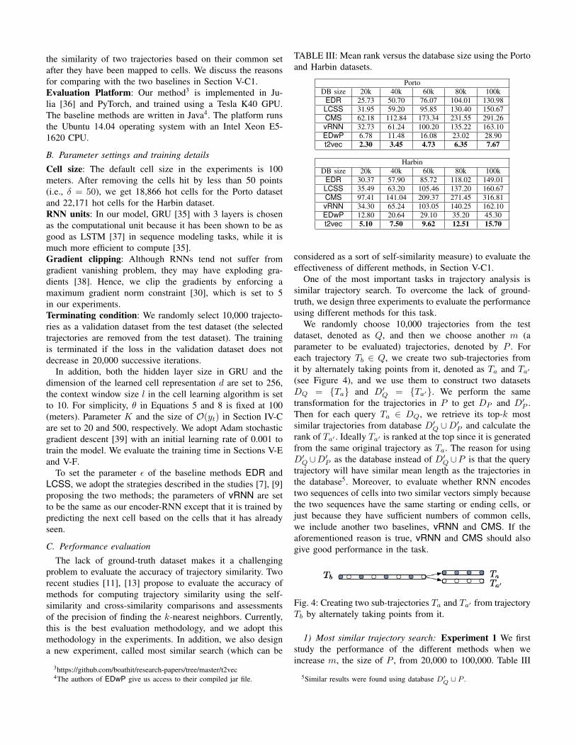
G. Effect of the training data size

In this experiment, we evaluate the effect of training datasize on the accuracy of the trajectory similarity search. Thesetting is similar to the one in Section V-E, with exceptionthat we vary the training data size and fix the dropping rater1 at 0.6.

Figure 7 shows the effect of the training data size on themost similar search on the Porto dataset. The mean rank dropsrapidly as we increase the training data size from 200,000 to600,000, and the decrease slows down when we continue toenlarge the training data size. When we increase the trainingdata size from 200,000 to 600,000, more transition patternscan be learned for representing the trajectories, and thus themodel quality is enhanced significantly. However, when wefurther increase the training data size, the marginal benefit ofusing larger training data is less pronounced.

VI. CONCLUSIONS AND FUTURE WORK

To the best of our knowledge, we present the first solutionfor using learning for creating representations of trajectoriesthat are well suited for use in trajectory similarity computation.Most existing methods for trajectory similarity computationmeasure similarity by means of pairwise point-matching,which may not capture the underlying route information ofthe trajectories, thus being sensitive to non-uniform and lowsampling rates, and noise sample points. Moreover, all ofthem have a quadratic time complexity. Motivated by these

observations, we propose a seq2seq-based method to learnrepresentations for trajectories that enable accurate and effi-cient trajectory similarity search that is robust to sampling ratevariations and noisy sample points. The method is evaluatedempirically with favorable results in terms of both accu-racy and efficiency. It consistently outperforms the baselinemethods by a large margin in the most similarity tasks. Themethod is at least one order of magnitude faster than theother methods, thus it can support big trajectory analysis andinteractive use while the competition cannot.

This work sheds light on several new research directions:1) Employing the learned representations to explore moredownstream tasks, e.g., trajectory clustering and popular-routes search. 2) Extending the proposed method to moregeneral time series data beyond trajectories. 3) Developingindexing techniques like Locality-Sensitive Hashing [41] tofurther speed up the proposed method.

Acknowledgments. This work is supported in part by theRapid-Rich Object Search (ROSE) Lab at Nanyang Techno-logical University. The ROSE Lab is supported by the NationalResearch Foundation, Prime Minister’s Office, Singapore, un-der its IDM Futures Funding Initiative, administered by theInteractive and Digital Media Programme Office. This workwas also supported by the MOE Tier-2 grant MOE2016-T2-1-137, MOE Tier-1 grant RG31/17, NSFC under the grant61772537, and a grant from Microsoft. C. S. Jensen wassupported by the DiCyPS project and by a grant from the ObelFamily Foundation. W. Wei was supported by NSFC under thegrant 61602197, NSF under the grant 2016CFB192.

REFERENCES

[1] Z. Li, J. Han, M. Ji, L. A. Tang, Y. Yu, B. Ding, J. Lee, andR. Kays, “Movemine: Mining moving object data for discovery ofanimal movement patterns,” ACM TIST, vol. 2, no. 4, pp. 37:1–37:32,2011.

[2] Z. Chen, H. T. Shen, and X. Zhou, “Discovering popular routes fromtrajectories,” in ICDE, 2011, pp. 900–911.

[3] C.-C. Hung, W.-C. Peng, and W.-C. Lee, “Clustering and aggregatingclues of trajectories for mining trajectory patterns and routes,” VLDBJ,vol. 24, no. 2, pp. 169–192, 2015.

[4] H. Jeung, M. L. Yiu, X. Zhou, C. S. Jensen, and H. T. Shen, “Discoveryof convoys in trajectory databases,” PVLDB, vol. 1, no. 1, pp. 1068–1080, 2008.

[5] X. Li, V. Ceikute, C. S. Jensen, and K.-L. Tan, “Effective online groupdiscovery in trajectory databases,” IEEE TKDE, vol. 25, no. 12, pp.2752–2766, 2013.

[6] B.-K. Yi, H. Jagadish, and C. Faloutsos, “Efficient retrieval of similartime sequences under time warping,” in ICDE, 1998, pp. 201–208.

[7] M. Vlachos, G. Kollios, and D. Gunopulos, “Discovering similar mul-tidimensional trajectories,” in ICDE, 2002, pp. 673–684.

[8] L. Chen and R. Ng, “On the marriage of lp-norms and edit distance,”in PVLDB, 2004, pp. 792–803.

[9] L. Chen, M. T. Ozsu, and V. Oria, “Robust and fast similarity searchfor moving object trajectories,” in SIGMOD, 2005, pp. 491–502.

[10] K. Zheng, Y. Zheng, X. Xie, and X. Zhou, “Reducing uncertainty oflow-sampling-rate trajectories,” in ICDE, 2012, pp. 1144–1155.

[11] S. Ranu, P. Deepak, A. D. Telang, P. Deshpande, and S. Raghavan,“Indexing and matching trajectories under inconsistent sampling rates,”in ICDE, 2015, pp. 999–1010.

[12] P. Banerjee, S. Ranu, and S. Raghavan, “Inferring uncertain trajectoriesfrom partial observations,” in ICDM, 2014, pp. 30–39.

[13] H. Su, K. Zheng, H. Wang, J. Huang, and X. Zhou, “Calibratingtrajectory data for similarity-based analysis,” in SIGMOD, 2013, pp.833–844.

[14] A. Graves, S. Fernandez, F. Gomez, and J. Schmidhuber, “Connection-ist temporal classification: labelling unsegmented sequence data withrecurrent neural networks,” in ICML, 2006, pp. 369–376.

[15] M. Gutmann and A. Hyvarinen, “Noise-contrastive estimation: A newestimation principle for unnormalized statistical models,” in AISTATS,2010, pp. 297–304.

[16] E. Frentzos, K. Gratsias, and Y. Theodoridis, “Index-based most similartrajectory search,” in ICDE, 2007, pp. 816–825.

[17] S. Sankararaman, P. K. Agarwal, T. Mølhave, J. Pan, and A. P.Boedihardjo, “Model-driven matching and segmentation of trajectories,”in SIGSPATIAL, 2013, pp. 234–243.

[18] H. Wang, H. Su, K. Zheng, S. Sadiq, and X. Zhou, “An effectivenessstudy on trajectory similarity measures,” in Australian Database Con-ference, 2013, pp. 13–22.

[19] T. Mikolov, K. Chen, G. Corrado, and J. Dean, “Efficient estimation ofword representations in vector space,” arXiv preprint arXiv:1301.3781,2013.

[20] Q. V. Le and T. Mikolov, “Distributed representations of sentences anddocuments.” in ICML, 2014, pp. 1188–1196.

[21] B. Perozzi, R. Al-Rfou, and S. Skiena, “Deepwalk: Online learning ofsocial representations,” in SIGKDD, 2014, pp. 701–710.

[22] J. Tang, M. Qu, M. Wang, M. Zhang, J. Yan, and Q. Mei, “Line: Large-scale information network embedding,” in WWW, 2015, pp. 1067–1077.

[23] K. Cho, B. Van Merrienboer, C. Gulcehre, D. Bahdanau, F. Bougares,H. Schwenk, and Y. Bengio, “Learning phrase representations usingrnn encoder-decoder for statistical machine translation,” arXiv preprintarXiv:1406.1078, 2014.

[24] I. Sutskever, O. Vinyals, and Q. V. Le, “Sequence to sequence learningwith neural networks,” in NIPS, 2014, pp. 3104–3112.

[25] O. Vinyals, Ł. Kaiser, T. Koo, S. Petrov, I. Sutskever, and G. Hinton,“Grammar as a foreign language,” in NIPS, 2015, pp. 2773–2781.

[26] R. Kiros, Y. Zhu, R. R. Salakhutdinov, R. Zemel, R. Urtasun, A. Tor-ralba, and S. Fidler, “Skip-thought vectors,” in NIPS, 2015, pp. 3294–3302.

[27] D. Williams and G. Hinton, “Learning representations by back-propagating errors,” Nature, vol. 323, no. 6088, pp. 533–538, 1986.

[28] P. J. Werbos, “Backpropagation through time: what it does and how todo it,” Proceedings of the IEEE, vol. 78, no. 10, pp. 1550–1560, 1990.

[29] Y. Bengio, R. Ducharme, P. Vincent, and C. Jauvin, “A neural proba-bilistic language model,” JMLR, vol. 3, pp. 1137–1155, 2003.

[30] A. Graves, “Generating sequences with recurrent neural networks,” arXivpreprint arXiv:1308.0850, 2013.

[31] R. H. Guting and M. Schneider, “Realm-based spatial data types: therose algebra,” VLDBJ, vol. 4, no. 2, pp. 243–286, 1995.

[32] Y. Bengio, A. Courville, and P. Vincent, “Representation learning: Areview and new perspectives,” TPAMI, vol. 35, no. 8, pp. 1798–1828,2013.

[33] D. Bahdanau, K. Cho, and Y. Bengio, “Neural machine translation byjointly learning to align and translate,” arXiv preprint arXiv:1409.0473,2014.

[34] T. Mikolov, I. Sutskever, K. Chen, G. S. Corrado, and J. Dean,“Distributed representations of words and phrases and their composi-tionality,” in NIPS, 2013, pp. 3111–3119.

[35] J. Chung, C. Gulcehre, K. Cho, and Y. Bengio, “Empirical evaluation ofgated recurrent neural networks on sequence modeling,” arXiv preprintarXiv:1412.3555, 2014.

[36] J. Bezanson, A. Edelman, S. Karpinski, and V. B. Shah, “Julia: A freshapproach to numerical computing,” SIAM review, vol. 59, no. 1, pp.65–98, 2017.

[37] S. Hochreiter and J. Schmidhuber, “Long short-term memory,” Neuralcomputation, vol. 9, no. 8, pp. 1735–1780, 1997.

[38] R. Pascanu, T. Mikolov, and Y. Bengio, “On the difficulty of trainingrecurrent neural networks,” in ICML (3), 2013, pp. 1310–1318.

[39] D. Kingma and J. Ba, “Adam: A method for stochastic optimization,”arXiv preprint arXiv:1412.6980, 2014.

[40] S. Jean, K. Cho, R. Memisevic, and Y. Bengio, “On using verylarge target vocabulary for neural machine translation,” arXiv preprintarXiv:1412.2007, 2014.

[41] A. Andoni and P. Indyk, “Near-optimal hashing algorithms for approxi-mate nearest neighbor in high dimensions,” in FOCS, 2006, pp. 459–468.

Documents

Deep Representation Learning for Trajectory Similarity