Embed Size (px)
Citation preview
Computational Fluid Dynamics
Computational Fluid Dynamics
R. Verfurth
Fakultat fur MathematikRuhr-Universitat Bochum
www.ruhr-uni-bochum.de/num1
Lecture Series / Milan / March 2010
1/ 300
Computational Fluid Dynamics
Contents
Fundamentals
Variational Formulation of the Stokes Equations
Discretization of the Stokes Equations
Solution of the Discrete Problems
A Posteriori Error Estimation and Adaptivity
Stationary Incompressible Navier-Stokes Equations
Non-Stationary Incompressible Navier-StokesEquations
Compressible and Inviscid Problems
References
2/ 300
Computational Fluid Dynamics
Fundamentals
Fundamentals
I Modelization
I Notations and Auxiliary Results
3/ 300
Computational Fluid Dynamics
Fundamentals
Modelization
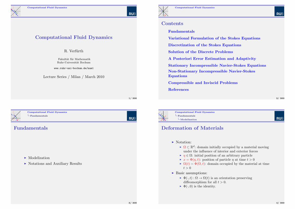
Deformation of Materials
I Notation:I Ω ⊂ Rd: domain initially occupied by a material moving
under the influence of interior and exterior forcesI η ∈ Ω: initial position of an arbitrary particleI x = Φ(η, t): position of particle η at time t > 0I Ω(t) = Φ(Ω, t): domain occupied by the material at timet > 0
I Basic assumptions:I Φ(·, t) : Ω→ Ω(t) is an orientation preserving
diffeomorphism for all t > 0.I Φ(·, 0) is the identity.
4/ 300
Computational Fluid Dynamics
Fundamentals
Modelization
Lagrange and Euler Representation
I Lagrange representation: Fix η and look at the trajectoryt 7→ Φ(η, t). η is called Lagrange coordinate. TheLangrange coordinate system moves with the fluid.
I Euler representation: Fix the point x and look at thetrajectory t 7→ Φ(·, t)−1(x) which passes through x. x iscalled Euler coordinate. The Euler coordinate system isfixed.
5/ 300
Computational Fluid Dynamics
Fundamentals
Modelization
Velocity
Velocity of the movement at the point x = Φ(η, t) is
v(x, t) =∂
∂tΦ(η, t).
6/ 300
Computational Fluid Dynamics
Fundamentals
Modelization
Properties
DΦ = (∂Φi∂ηj
)1≤i,j≤d Jacobi matrix of Φ, J = detDΦ Jacobi
determinant of Φ, Aij co-factors of DΦ (1 ≤ i, j ≤ d):
∂
∂tJ =
∑i,j
∂
∂(DΦ)ijJ∂
∂t(DΦ)ij =
∑i,j
(−1)i+jAij∂2
∂t∂ηjΦi
=∑i,j
(−1)i+jAij∂
∂ηjvi =
∑i,j,k
(−1)i+jAij∂
∂ηjΦk
∂
∂xkvi
=∑i,k
Jδi,k∂
∂xkvi = J divv
7/ 300
Computational Fluid Dynamics
Fundamentals
Modelization
Transport Theorem
d
dt
∫V (t)
f(x, t)dx
=d
dt
∫Vf(Φ(η, t), t)J(η, t)dη
=
∫V
( ∂∂tf(Φ(η, t), t)J(η, t)
+∇f(Φ(η, t), t) · v(Φ(η, t), t)J(η, t)
+ f(Φ(η, t), t) divv(Φ(η, t), t)J(η, t))dη
=
∫V (t)
( ∂∂tf(x, t) + div
[f(x, t)v(x, t)
])dx
8/ 300
Computational Fluid Dynamics
Fundamentals
Modelization
Conservation of Mass
I ρ denotes the density of the material.
I
∫V (t)
ρdx is the total mass of a control volume.
I Total mass is conserved:
0 =d
dt
∫V (t)
ρdx =
∫V (t)
( ∂∂tρ+ div
[ρv])dx.
I This holds for every control volume, hence:
∂
∂tρ+ div
[ρv]
= 0.
9/ 300
Computational Fluid Dynamics
Fundamentals
Modelization
Conservation of Momentum
I
∫V (t)
ρvdx is the total momentum of a control volume.
I Its temporal change is
d
dt
∫V (t)
ρvdx =
∫V (t)
( ∂∂t
[ρv]
+ div[ρv ⊗ v
])dx.
I This is in equilibrium with exterior and interior forces.
I Exterior forces are given by
∫V (t)
ρfdx.
10/ 300
Computational Fluid Dynamics
Fundamentals
Modelization
Interior Forces
Basic assumptions:
I Interior forces act via the surface of a volume V (t).
I Interior forces only depend on the normal direction of thesurface of the volume.
I Interior forces are additive and continuous.
11/ 300
Computational Fluid Dynamics
Fundamentals
Modelization
Cauchy Theorem
The previous assumptions imply:
I There is a tensor field T : Ω→ Rd×d such that the interior
forces are given by
∫∂V (t)
T · ndS.
I T is such that the divergence theorem of Gauß holds∫∂V (t)
T · ndS =
∫V (t)
divTdx.
12/ 300
Computational Fluid Dynamics
Fundamentals
Modelization
Conservation of Momentum (ctd.)
I The conservation of momentum and the Cauchy theoremimply:∫
V (t)
( ∂∂t
(ρv) + div(ρv ⊗ v))
=
∫V (t)
(ρf + divT
).
I This holds for every control volume, hence:
∂
∂t(ρv) + div(ρv ⊗ v) = ρf + divT.
13/ 300
Computational Fluid Dynamics
Fundamentals
Modelization
Conservation of Energy
I
∫V (t)
edx is the total energy of a control volume.
I Its temporal change is in equilibrium with the internalenergy and the energy of exterior and interior forces.
I Exterior forces contribute
∫V (t)
ρf · vdx.
I Interior forces give
∫∂V (t)
n ·T · vdS =
∫V (t)
div[T · v
]dx.
I The Cauchy theorem implies that the internal energy is of
the form
∫∂V (t)
n · σdS =
∫V (t)
divσdx.
I Hence, conservation of energy implies
∂
∂te+ div(ev) = ρf · v + div(T · v) + divσ.
14/ 300
Computational Fluid Dynamics
Fundamentals
Modelization
Constitutive Laws
Basic assumptions:
I T only depends on the gradient of the velocity.
I The dependence on the velocity gradient is linear.
I T is symmetric.
(Due to the Cauchy theorem this is a consequence of theconservation of angular momentum.)
I In the absence of internal friction, T is diagonal andproportional to the pressure, i.e. all interior forces act innormal direction.
I The total energy e is the sum of internal and kinetic energy.
I σ is proportional to the variation of the internal energy.
15/ 300
Computational Fluid Dynamics
Fundamentals
Modelization
Consequences of the Constitutive Laws
Above assumptions imply:
I T = 2λD(v) + µ(divv) I− pI,where D(v) = 1
2(∇v +∇vt) is the deformation tensor, λ, µare the dynamic viscosities, p is the pressure, I is the unittensor.
I e = ρε+ 12ρ|v|
2,
where ε is often identified with the temperature.
I σ = α∇ε.
16/ 300
Computational Fluid Dynamics
Fundamentals
Modelization
Compressible Navier-Stokes Equations inConservative Form
∂
∂tρ+ div(ρv) = 0
∂
∂t(ρv) + div(ρv ⊗ v) = ρf + 2λdivD(v)
+ µ grad divv − grad p
∂
∂te+ div(ev) = ρf · v + 2λ div[D(v) · v]
+ µdiv[divv · v]− div(pv) + α∆ε
p = p(ρ, ε)
e = ρε+1
2ρ|v|2
17/ 300
Computational Fluid Dynamics
Fundamentals
Modelization
Euler Equations
Inviscid flows, i.e. λ = µ = 0:
∂
∂tρ+ div(ρv) = 0
∂
∂t(ρv) + div(ρv ⊗ v + pI) = ρf
∂
∂te+ div(ev + pv) = ρf · v + α∆ε
p = p(ρ, ε)
e = ρε+1
2ρ|v|2
18/ 300
Computational Fluid Dynamics
Fundamentals
Modelization
Compressible Navier-Stokes Equations inNon-Conservative Form
Insert first equation in second one and first and second equationin third one:
∂
∂tρ+ div(ρv) = 0
ρ[∂
∂tv + (v · ∇)v] = ρf + λ∆v + (λ+ µ) grad divv − grad p
ρ[∂
∂tε+ ρv · grad ε] = λD(v) : D(v) + µ(divv)2 − p divv
+ α∆ε
p = p(ρ, ε)
19/ 300
Computational Fluid Dynamics
Fundamentals
Modelization
Non-Stationary Incompressible Navier-StokesEquations
I Assume that the density ρ is constant,
I replace p by pρ ,
I denote by ν = λρ the kinematic viscosity,
I drop the energy equation:
divv = 0
∂
∂tv + (v · ∇)v = f + ν∆v − grad p
20/ 300
Computational Fluid Dynamics
Fundamentals
Modelization
Reynolds’ Number
I Introduce a reference length L, a reference time T , areference velocity U , a reference pressure P , and areference force F and new variables and quantities byx = Ly, t = Tτ , v = Uu, p = Pq, f = Fg.
I Choose T , F and P such that T = LU , F = νU
L2 and PLνU = 1.
I Then
divu = 0
∂
∂tu +Re(u · ∇)u = f + ∆u− grad q,
where Re = LUν is the dimensionless Reynolds’ number.
21/ 300
Computational Fluid Dynamics
Fundamentals
Modelization
Stationary Incompressible Navier-StokesEquations
Assume that the flow is stationary:
divv = 0
−ν∆v + (v · ∇)v + grad p = f
22/ 300
Computational Fluid Dynamics
Fundamentals
Modelization
Stokes Equations
Linearize at velocity v = 0:
divv = 0
−∆v + grad p = f
23/ 300
Computational Fluid Dynamics
Fundamentals
Modelization
Boundary Conditions
I Around 1827, Pierre Louis Marie Henri Navier suggestedthe general boundary condition
λnv · n + (1− λn)n ·T · n = 0
λt[v − (v · n)n] + (1− λt)[T · n− (n ·T · n)n] = 0
with parameters λn, λt ∈ [0, 1] depending on the actualflow-problem.
I A particular case is the slip boundary conditionv · n = 0, T · n− (n ·T · n)n = 0.
I Around 1845, Sir George Gabriel Stokes suggested theno-slip boundary condition v = 0.
24/ 300
Computational Fluid Dynamics
Fundamentals
Notations and Auxiliary Results
Sobolev Spaces and Norms
I L2(Ω) Lebesgue space with norm ‖ϕ‖Ω = ‖ϕ‖ =∫
Ω ϕ2 1
2
I Hk(Ω) = ϕ ∈ L2(Ω) : Dαϕ ∈ L2(Ω)∀α1 + . . .+ αd ≤ k,k ≥ 1, Sobolev spaces with semi-norm
|ϕ|k,Ω = |ϕ|k =∑
α1+...+αd=k‖Dαϕ‖2 1
2and norm
‖ϕ‖k,Ω = ‖ϕ‖k =∑k
`=0|ϕ|2` 1
2
I Norms of vector- or tensor-valued functions are definedcomponent-wise.
I H10 (Ω) = ϕ ∈ H1(Ω) : ϕ = 0 on Γ = ∂Ω
I V = v ∈ H10 (Ω)d : divv = 0
I L20(Ω) = ϕ ∈ L2(Ω) :
∫Ω ϕ = 0
25/ 300
Computational Fluid Dynamics
Fundamentals
Notations and Auxiliary Results
Poincare, Friedrichs and Trace Inequalities
I Poincare inequality: ‖ϕ‖ ≤ cP diam(Ω)|ϕ|1 for allϕ ∈ H1(Ω) ∩ L2
0(Ω)
I cP = 1π if Ω is convex.
I Friedrichs inequality: ‖ϕ‖ ≤ cF diam(Ω)|ϕ|1 for allϕ ∈ H1
0 (Ω)
I Trace inequality: ‖ϕ‖Γ ≤cT,1(Ω)‖ϕ‖2 + cT,2(Ω)|ϕ|21
12
for
all ϕ ∈ H1(Ω)
I cT,1(Ω) ≈ diam(Ω)−1, cT,2(Ω) ≈ diam(Ω) if Ω is a simplexor parallelepiped
26/ 300
Computational Fluid Dynamics
Fundamentals
Notations and Auxiliary Results
Finite Element Meshes T
I Ω ∪ Γ is the union of all elements in T .
I Affine equivalence: Each K ∈ T is either a triangle or aparallelogram, if d = 2, or a tetrahedron or aparallelepiped, if d = 3.
I Admissibility: Any two elements in T are either disjoint orshare a vertex or a complete edge or – if d = 3 – a completeface.
I Shape-regularity: For every element K, the ratio of itsdiameter hK to the diameter ρK of the largest ballinscribed into K is bounded independently of K.
I Mesh-size: h = hT = maxK∈T
hK
27/ 300
Computational Fluid Dynamics
Fundamentals
Notations and Auxiliary Results
Finite Element Spaces
I Rk(K) =
spanxα1
1 · . . . · xαdd : α1 + . . .+ αd ≤ k
if K is a triangle or a tetrahedronspanxα1
1 · . . . · xαdd : maxα1, . . . , αd ≤ k
if K is a parallelogram or a parallelepiped
I Sk,−1(T ) = ϕ : Ω→ R : ϕ∣∣K∈ Rk(K) ∀K ∈ T
I Sk,0(T ) = Sk,−1(T ) ∩ C(Ω)
I Sk,00 (T ) = Sk,0(T ) ∩H10 (Ω)
= ϕ ∈ Sk,0(T ) : ϕ = 0 on Γ
28/ 300
Computational Fluid Dynamics
Fundamentals
Notations and Auxiliary Results
Approximation Properties
I infϕT ∈Sk,−1(T )
‖ϕ− ϕT ‖ ≤ chk+1|ϕ|k+1
ϕ ∈ Hk+1(Ω), k ∈ NI inf
ϕT ∈Sk,0(T )|ϕ− ϕT |j ≤ chk+1−j |ϕ|k+1
ϕ ∈ Hk+1(Ω), j ∈ 0, 1, k ∈ N∗
I infϕT ∈Sk,00 (T )
|ϕ− ϕT |j ≤ chk+1−j |ϕ|k+1
ϕ ∈ Hk+1(Ω) ∩H10 (Ω),
j ∈ 0, 1, k ∈ N∗
29/ 300
Computational Fluid Dynamics
Fundamentals
Notations and Auxiliary Results
Vertices and Faces
I N : set of all element vertices
I E : set of all (d− 1)-dimensional element faces
I A subscript K, Ω or Γ to N or E indicates that only thosevertices or faces are considered that are contained in therespective set.
30/ 300
Computational Fluid Dynamics
Fundamentals
Notations and Auxiliary Results
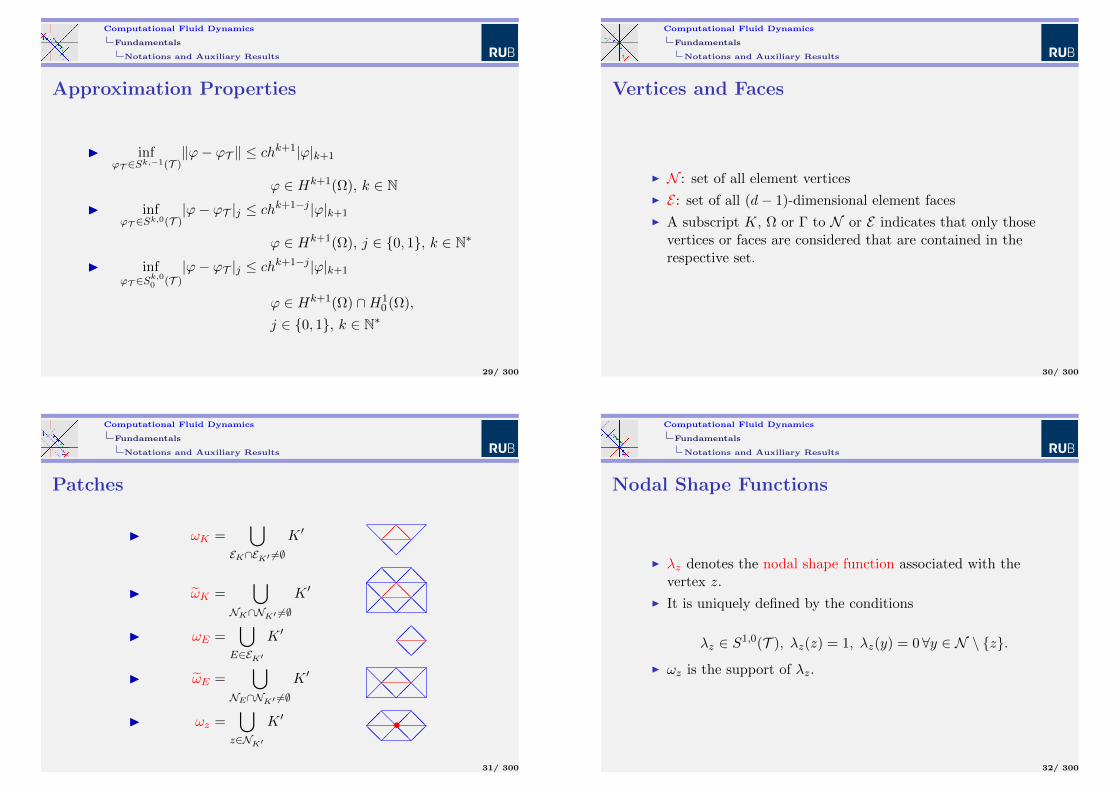
Patches
I ωK =⋃
EK∩EK′ 6=∅
K ′ @@@
@@
I ωK =⋃
NK∩NK′ 6=∅
K ′@@@@@@@@
@@
@@
I ωE =⋃
E∈EK′
K ′ @@@@
I ωE =⋃
NE∩NK′ 6=∅
K ′
@@@
@@@
I ωz =⋃
z∈NK′
K ′ @@@
@@@@
•
31/ 300
Computational Fluid Dynamics
Fundamentals
Notations and Auxiliary Results
Nodal Shape Functions
I λz denotes the nodal shape function associated with thevertex z.
I It is uniquely defined by the conditions
λz ∈ S1,0(T ), λz(z) = 1, λz(y) = 0∀y ∈ N \ z.
I ωz is the support of λz.
32/ 300
Computational Fluid Dynamics
Fundamentals
Notations and Auxiliary Results
A Quasi-Interpolation Operator
I Define the quasi-interpolation operatorRT : L1(Ω)→ S1,0
0 (T ) by
RT ϕ =∑z∈NΩ
λzϕz with ϕz =
∫ωzϕdx∫
ωzdx
.
I It has the following local approximation properties for allϕ ∈ H1
0 (Ω)
‖ϕ−RT ϕ‖K ≤ cA1hK |ϕ|1,ωK
‖ϕ−RT ϕ‖∂K ≤ cA2h12K |ϕ|1,ωK .
33/ 300
Computational Fluid Dynamics
Fundamentals
Notations and Auxiliary Results
Proof of the Local Approximation Properties
I The Poincare inequality implies for every vertex z‖ϕ− ϕz‖ωz ≤ cz diam(ωz)|ϕ|1,ωz .
I The trace inequality yields for all faces E of all elements K
‖ϕ‖E ≤ c1h− 1
2K ‖ϕ‖K + c2h
12K |ϕ|1,K .
I The properties of the nodal shape functions imply
‖ϕ−RT ϕ‖K ≤∑z∈NK
‖ϕ− ϕz‖K +∑
z∈NK,Γ
‖ϕz‖K .
I The first term is bounded using the Poincare inequality,the second one using ϕ ∈ H1
0 (Ω).
34/ 300
Computational Fluid Dynamics
Fundamentals
Notations and Auxiliary Results
Bubble Functions
I Define element and face bubble functions by
ψK = αK∏z∈NK
λz, ψE = αE∏z∈NE
λz.
I The weights αK and αE are determined by the conditions
maxx∈K
ψK(x) = 1, maxx∈E
ψE(x) = 1.
I K is the support of ψK ; ωE is the support of ψE .
35/ 300
Computational Fluid Dynamics
Fundamentals
Notations and Auxiliary Results
Inverse Estimates for the Bubble Functions
For all elements K, all faces E and all polynomials ϕ thefollowing inverse estimates are valid
cI1,k‖ϕ‖K ≤ ‖ψ12Kϕ‖K ,
‖∇(ψKϕ)‖K ≤ cI2,kh−1K ‖ϕ‖K ,
cI3,k‖ϕ‖E ≤ ‖ψ12Eϕ‖E ,
‖∇(ψEϕ)‖ωE ≤ cI4,kh− 1
2E ‖ϕ‖E ,
‖ψEϕ‖ωE ≤ cI5,kh12E‖ϕ‖E .
36/ 300
Computational Fluid Dynamics
Fundamentals
Notations and Auxiliary Results
Proof of the Inverse Estimates
I Transform the left hand-sides to the reference simplex orcube.
I Take into account that the left-hand sides definesemi-norms.
I Invoke the equivalence of norms on finite dimensionalspaces to prove the corresponding estimates on thereference element.
I Transform the right-hand sides back to the current elementor face.
37/ 300
Computational Fluid Dynamics
Fundamentals
Notations and Auxiliary Results
Jumps
I nE : a unit vector perpendicular to a given face E
I [ϕ]E : jump of a given piece-wise continuous function acrossa given face E in the direction of nE
I [ϕ]E depends on the orientation of nE but quantities of theform [nE · ∇ϕ]E are independent thereof.
38/ 300
Computational Fluid Dynamics
Variational Formulation of the Stokes Equations
Variational Formulation of the Stokes Equations
I A First Attempt
I Abstract Saddle-Point Problems
I Saddle-Point Formulation of the Stokes Equations
39/ 300
Computational Fluid Dynamics
Variational Formulation of the Stokes Equations
A First Attempt
A Variational Formulation of the StokesEquations
I Stokes equations with no-slip boundary condition
−∆u + grad p = f in Ω, divu = 0 in Ω, u = 0 on Γ
I Multiply momentum equation withv ∈ V = w ∈ H1
0 (Ω)d : divw = 0, integrate over Ω anduse integration by parts.
I Resulting variational formulation:
Find u ∈ V such that for all v ∈ V∫Ω∇u : ∇v =
∫Ωf · v
40/ 300
Computational Fluid Dynamics
Variational Formulation of the Stokes Equations
A First Attempt
Corresponding Discretization
I Find uT ∈ V (T ) ⊂ V such that for all vT ∈ V (T )∫Ω∇uT : ∇vT =
∫Ωf · vT
I Advantage:
The discrete problem is symmetric positive definite.
I Disadvantage:
The discrete problem gives no information on the pressure.
I Candidate for lowest order discretization:
V (T ) = S1,00 (T )d ∩ V .
41/ 300
Computational Fluid Dynamics
Variational Formulation of the Stokes Equations
A First Attempt
The Space V (T ) = S1,00 (T )d ∩ V
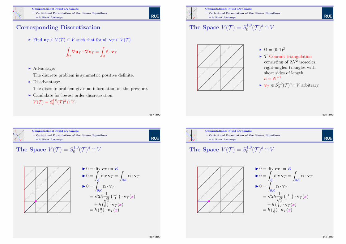
I Ω = (0, 1)2
I T Courant triangulationconsisting of 2N2 isoscelesright-angled triangles withshort sides of lengthh = N−1
I vT ∈ S1,00 (T )d ∩ V arbitrary
42/ 300
Computational Fluid Dynamics
Variational Formulation of the Stokes Equations
A First Attempt
The Space V (T ) = S1,00 (T )d ∩ V
•
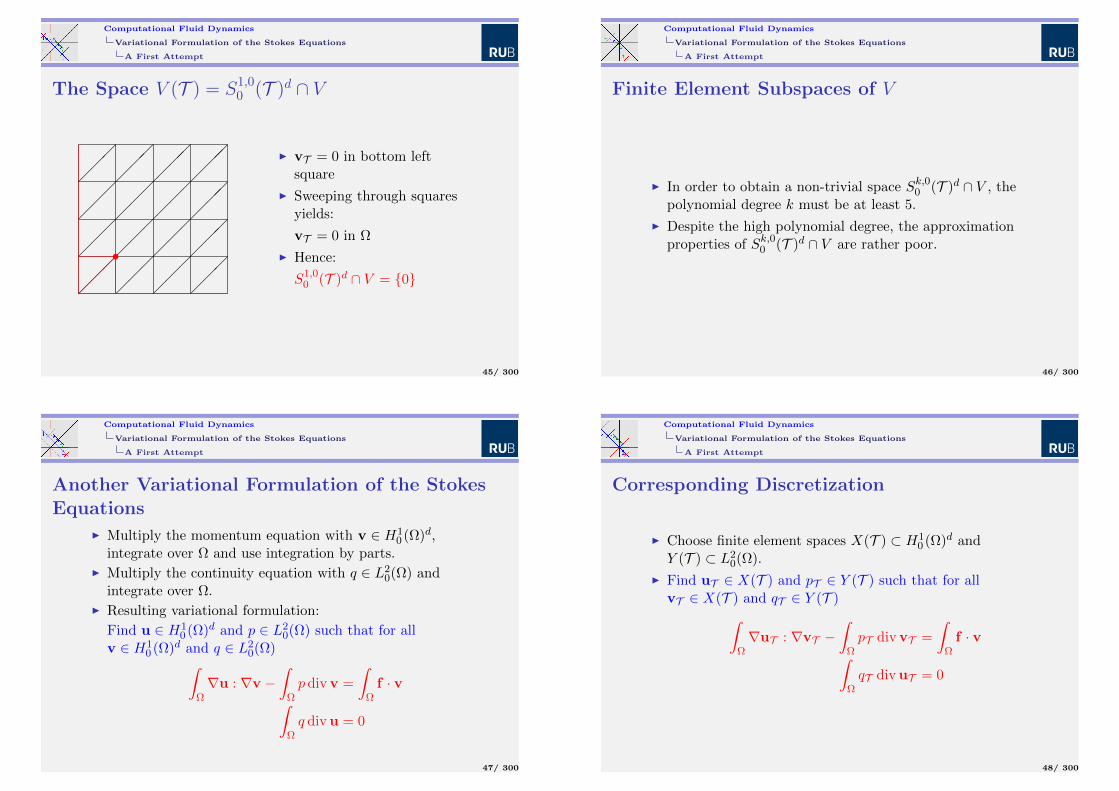
I 0 = divvT on K
I 0 =
∫K
divvT =
∫∂K
n · vT
I 0 =
∫∂K
n · vT
=√
2h1√2
(−11
)· vT (x)
+ h ( 10 ) · vT (x)
= h ( 01 ) · vT (x)
43/ 300
Computational Fluid Dynamics
Variational Formulation of the Stokes Equations
A First Attempt
The Space V (T ) = S1,00 (T )d ∩ V
•
I 0 = divvT on K
I 0 =
∫K
divvT =
∫∂K
n · vT
I 0 =
∫∂K
n · vT
=√
2h1√2
(1−1
)· vT (x)
+ h ( 01 ) · vT (x)
= h ( 10 ) · vT (x)
44/ 300
Computational Fluid Dynamics
Variational Formulation of the Stokes Equations
A First Attempt
The Space V (T ) = S1,00 (T )d ∩ V
•
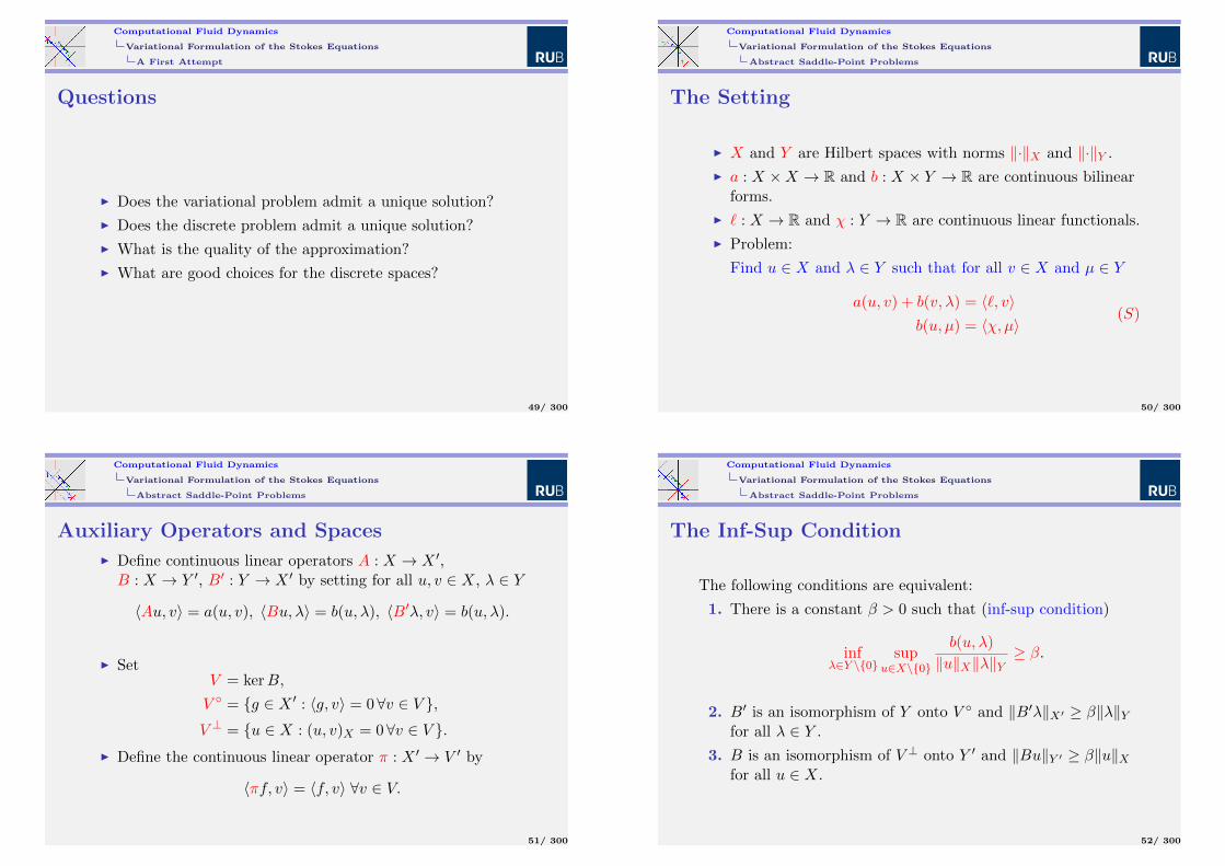
I vT = 0 in bottom leftsquare
I Sweeping through squaresyields:
vT = 0 in Ω
I Hence:
S1,00 (T )d ∩ V = 0
45/ 300
Computational Fluid Dynamics
Variational Formulation of the Stokes Equations
A First Attempt
Finite Element Subspaces of V
I In order to obtain a non-trivial space Sk,00 (T )d ∩ V , thepolynomial degree k must be at least 5.
I Despite the high polynomial degree, the approximationproperties of Sk,00 (T )d ∩ V are rather poor.
46/ 300
Computational Fluid Dynamics
Variational Formulation of the Stokes Equations
A First Attempt
Another Variational Formulation of the StokesEquations
I Multiply the momentum equation with v ∈ H10 (Ω)d,
integrate over Ω and use integration by parts.
I Multiply the continuity equation with q ∈ L20(Ω) and
integrate over Ω.
I Resulting variational formulation:
Find u ∈ H10 (Ω)d and p ∈ L2
0(Ω) such that for allv ∈ H1
0 (Ω)d and q ∈ L20(Ω)∫
Ω∇u : ∇v −
∫Ωp divv =
∫Ωf · v∫
Ωq divu = 0
47/ 300
Computational Fluid Dynamics
Variational Formulation of the Stokes Equations
A First Attempt
Corresponding Discretization
I Choose finite element spaces X(T ) ⊂ H10 (Ω)d and
Y (T ) ⊂ L20(Ω).
I Find uT ∈ X(T ) and pT ∈ Y (T ) such that for allvT ∈ X(T ) and qT ∈ Y (T )∫
Ω∇uT : ∇vT −
∫ΩpT divvT =
∫Ωf · v∫
ΩqT divuT = 0
48/ 300
Computational Fluid Dynamics
Variational Formulation of the Stokes Equations
A First Attempt
Questions
I Does the variational problem admit a unique solution?
I Does the discrete problem admit a unique solution?
I What is the quality of the approximation?
I What are good choices for the discrete spaces?
49/ 300
Computational Fluid Dynamics
Variational Formulation of the Stokes Equations
Abstract Saddle-Point Problems
The Setting
I X and Y are Hilbert spaces with norms ‖·‖X and ‖·‖Y .
I a : X ×X → R and b : X × Y → R are continuous bilinearforms.
I ` : X → R and χ : Y → R are continuous linear functionals.
I Problem:
Find u ∈ X and λ ∈ Y such that for all v ∈ X and µ ∈ Y
a(u, v) + b(v, λ) = 〈`, v〉b(u, µ) = 〈χ, µ〉
(S)
50/ 300
Computational Fluid Dynamics
Variational Formulation of the Stokes Equations
Abstract Saddle-Point Problems
Auxiliary Operators and Spaces
I Define continuous linear operators A : X → X ′,B : X → Y ′, B′ : Y → X ′ by setting for all u, v ∈ X, λ ∈ Y
〈Au, v〉 = a(u, v), 〈Bu, λ〉 = b(u, λ), 〈B′λ, v〉 = b(u, λ).
I SetV = kerB,
V = g ∈ X ′ : 〈g, v〉 = 0∀v ∈ V ,V ⊥ = u ∈ X : (u, v)X = 0∀v ∈ V .
I Define the continuous linear operator π : X ′ → V ′ by
〈πf, v〉 = 〈f, v〉 ∀v ∈ V.
51/ 300
Computational Fluid Dynamics
Variational Formulation of the Stokes Equations
Abstract Saddle-Point Problems
The Inf-Sup Condition
The following conditions are equivalent:
1. There is a constant β > 0 such that (inf-sup condition)
infλ∈Y \0
supu∈X\0
b(u, λ)
‖u‖X‖λ‖Y≥ β.
2. B′ is an isomorphism of Y onto V and ‖B′λ‖X′ ≥ β‖λ‖Yfor all λ ∈ Y .
3. B is an isomorphism of V ⊥ onto Y ′ and ‖Bu‖Y ′ ≥ β‖u‖Xfor all u ∈ X.
52/ 300
Computational Fluid Dynamics
Variational Formulation of the Stokes Equations
Abstract Saddle-Point Problems
Motivation of the Inf-Sup Condition
Assume that X = Rn, Y = Rm with m < n and b(u, λ) = λTBuwith a rectangular matrix B ∈ Rm×n. Then the followingconditions are equivalent:
I B has maximal rang m.
I The rows of B are linearly independent.
I λTBu = 0 for all u ∈ Rn implies λ = 0.
I infλ supuλTBu|u||λ| > 0.
I The linear system BTλ = 0 only admits the trivial solution.
I For every f ∈ Rm there is a unique u ∈ Rn which isorthogonal to kerB and which satisfies Bu = f .
53/ 300
Computational Fluid Dynamics
Variational Formulation of the Stokes Equations
Abstract Saddle-Point Problems
Proof of the Equivalences
1.⇒ 2. Condition (1), the definition of B′ and ‖·‖X′ imply
‖B′λ‖X′ = supu∈X\0
b(u, λ)
‖u‖X≥ β‖λ‖Y .
Hence, B′ is injective and its range is closed. The closedgraph theorem then proves (2).
2.⇒ 1. This is a consequence of the above equality.
2.⇔ 3. From the definitions of V and V ⊥ one concludes that V
and (V ⊥)′ are isometric. Hence, B is an isomorphism ofV ⊥ onto Y ′ if and only if B′ is an isomorphism of(Y ′)′ ' Y onto (V ⊥)′ ' V and both isomorphisms havethe same norm.
54/ 300
Computational Fluid Dynamics
Variational Formulation of the Stokes Equations
Abstract Saddle-Point Problems
Well-Posedness of Problem (S)
I Problem (S) admits a unique solution for every right-handside if and only if
(i) πA is an isomorphism of V onto V ′ and(ii) b satisfies the inf-sup condition.
I If problem (S) is well-posed, its solution satisfies
‖u‖X + ‖λ‖Y ≤ c‖`‖X′ + ‖χ‖Y ′
.
The constant c grows with β−1.
55/ 300
Computational Fluid Dynamics
Variational Formulation of the Stokes Equations
Abstract Saddle-Point Problems
Proof of “⇐ ”
I Due to (ii) there is a unique u0 ∈ V ⊥ with Bu0 = χ and‖u0‖X ≤ 1
β‖χ‖Y ′ .I Due to (i) there is a unique w ∈ V with πAw = π(`−Au0)
and ‖w‖X ≤ ‖(πA)−1‖L(V ′,V )‖`−Au0‖X′ .I u = u0 + w satisfies π(`−Au) = 0 whence `−Au ∈ V .I Due to (ii) there is a unique λ ∈ Y with B′λ = `−Au and‖λ‖Y ≤ 1
β‖`−Au‖X′ .I u, λ solve (S) and satisfy the stability estimate.
56/ 300
Computational Fluid Dynamics
Variational Formulation of the Stokes Equations
Abstract Saddle-Point Problems
Proof of “⇒ ”I Problem (S) with ` = 0 and arbitrary χ ∈ Y ′ admits a
unique solution. Hence Y ′ = rangeB. The open mappingtheorem proves that B is an isomorphism and thusestablishes (ii).
I Consider a u ∈ V with πAu = 0. Due to (ii), there is aunique λ ∈ Y with B′λ = −Au. Thus u, λ solve (S) withhomogeneous right-hand side. Hence, u = 0 and πA isinjective.
I Due to the Hahn-Banach theorem, for every g ∈ V ′, thereis an ` ∈ X ′ with π` = g. Problem (S) admits a uniquesolution u, λ for the right-hand side `, χ = 0. Hence, thereis a u ∈ X with πAu = g and πA is surjective.
I The open mapping theorem proves that πA is anisomorphism and thus establishes (i).
57/ 300
Computational Fluid Dynamics
Variational Formulation of the Stokes Equations
Abstract Saddle-Point Problems
Coercive Forms a
Assume that a is symmetric and coercive on X, i.e. there is anα > 0 such that a(u, u) ≥ α‖u‖2X holds for all u ∈ X. Then:
I πA is an isomorphism and ‖(πA)−1‖L(V ′,V ) ≤ 1α .
I Problem (S) is well-posed if and only if the form b satisfiesthe inf-sup condition.
I The solution of problem (S) is the unique saddle-point ofthe functional L(u, λ) = 1
2a(u, u) + b(u, λ)− 〈`, u〉 − 〈χ, λ〉.I The solution u of (S) minimizes the functionalJ(u) = 1
2a(u, u)− 〈`, u〉 under the constraintb(u, µ) = 〈χ, µ〉 for all µ ∈ Y .
58/ 300
Computational Fluid Dynamics
Variational Formulation of the Stokes Equations
Abstract Saddle-Point Problems
Discretization of Saddle-Point Problems
I Replace X and Y by finite dimensional subspaces Xn andYn.
I Resulting discrete problem:
Find un ∈ Xn and λn ∈ Yn such that for all vn ∈ Xn andµn ∈ Yn
a(un, vn) + b(vn, λn) = 〈`, vn〉b(un, µn) = 〈χ, µn〉
(Sn)
59/ 300
Computational Fluid Dynamics
Variational Formulation of the Stokes Equations
Abstract Saddle-Point Problems
Well-Posedness of Problem (Sn)
Assume for simplicity that the form a is coercive on X. Then:
I Problem (Sn) is well posed if and only if the form b satisfiesthe discrete inf-sup condition
infλn∈Yn\0
supun∈Xn\0
b(un, λn)
‖un‖X‖λn‖Y≥ βn > 0.
I If problem (Sn) is well-posed, its solution satisfies
‖un‖X + ‖λn‖Y ≤ c‖`‖X′ + ‖χ‖Y ′
.
The constant c grows with β−1n .
60/ 300
Computational Fluid Dynamics
Variational Formulation of the Stokes Equations
Abstract Saddle-Point Problems
Error Estimates
I Assume that a is coercive and that b satisfies both theinf-sup condition and the discrete inf-sup condition.
I Denote by u, λ the unique solution of problem (S) and byun, λn the unique solution of problem (Sn).
I Then there is a constant c which grows with β−1n such that
‖u− un‖X + ‖λ− λn‖Y
≤ c
infvn∈Xn
‖u− vn‖X + infµn∈Yn
‖λ− µn‖Y
61/ 300
Computational Fluid Dynamics
Variational Formulation of the Stokes Equations
Abstract Saddle-Point Problems
Proof of the Error EstimatesI For any vn ∈ Xn, µn ∈ Yn define ˜∈ X ′, χ ∈ Y ′ by
〈˜, v〉 = a(u− vn, v) + b(v, λ− µn),
〈χ, µ〉 = b(u− vn, µ).
I Then ‖˜‖X′ + ‖χ‖Y ′ ≤ c‖u− vn‖X + ‖λ− µn‖Y
.I Subtracting problems (S) and (Sn) gives for every wn ∈ Xn
and ρn ∈ Yn〈˜, wn〉 = a(un − vn, wn) + b(wn, λn − µn),
〈χ, ρn〉 = b(un − vn, ρn).
I The stability estimate for problem (Sn) and the triangleinequality now prove the error estimate.
62/ 300
Computational Fluid Dynamics
Variational Formulation of the Stokes Equations
Abstract Saddle-Point Problems
A Duality Argument
I H is another Hilbert space with norm ‖·‖H such that X isdense in H with continuous injection.
I For every g ∈ H denote by ug, λg the solution of problem(S) with ` = g and χ = 0.
I Then u and un satisfy the error estimate
‖u− un‖H≤ c‖u− un‖X + ‖λ− λn‖Y
·
· supg∈H\0
1
‖g‖H
inf
vn∈Xn‖u− vn‖X + inf
µn∈Yn‖λ− µn‖Y
.
63/ 300
Computational Fluid Dynamics
Variational Formulation of the Stokes Equations
Abstract Saddle-Point Problems
ProofI The density of X in H implies
‖u− un‖H = supg∈H\0
(g, u− un)H‖g‖H
.
I Subtracting (S) and (Sn) and using the definition of ug, λgyields for every vn ∈ Xn, µn ∈ Yn
(g, u− un)H
= a(u− un, ug) + b(u− un, λg) + b(ug, λ− λn)︸ ︷︷ ︸=0
= a(u− un, ug − vn) + b(ug − vn, λ− λn) + b(u− un, λg − µn)
+ a(u− un, vn) + b(vn, λ− λn)︸ ︷︷ ︸=0
+ b(u− un, µn)︸ ︷︷ ︸=0
.
64/ 300
Computational Fluid Dynamics
Variational Formulation of the Stokes Equations
Saddle-Point Formulation of the Stokes Equations
Saddle-Point Formulation of the StokesEquations
I The saddle-point formulation of the Stokes equations fitsinto the abstract framework with:
I X = H10 (Ω)d, Y = L2
0(Ω), H = L2(Ω)d
I a(u,v) =
∫Ω
∇u : ∇v, b(u, p) = −∫
Ω
pdivu
I 〈`,v〉 =
∫Ω
f · v, χ = 0
I The bilinear form a is coercive on X. Hence, we only haveto ascertain the inf-sup condition
infp∈L2
0(Ω)\0sup
u∈H10 (Ω)d\0
∫Ωp divu
|u|1‖p‖≥ β > 0.
65/ 300
Computational Fluid Dynamics
Variational Formulation of the Stokes Equations
Saddle-Point Formulation of the Stokes Equations
A Proof in R2
I Assume that Ω ⊂ R2 is either convex or has a C2 boundary.I Choose an arbitrary p ∈ L2
0(Ω).I Set v = ∇ϕ where ϕ ∈ H2(Ω) ∩ L2
0(Ω) is the unique weaksolution of the Neumann problem
∆ϕ = p in Ω,∂ϕ
∂n= 0 on Γ.
I Set w = ( ∂ψ∂x2,− ∂ψ
∂x1) where ψ ∈ H2(Ω) is the unique weak
solution of the biharmonic equation
∆2ψ = 0 in Ω, ψ = 0 on Γ,∂ψ
∂n= v · t on Γ.
I Set u = v + w. Then divu = p and |u|1 ≤ c‖p‖.66/ 300
Computational Fluid Dynamics
Variational Formulation of the Stokes Equations
Saddle-Point Formulation of the Stokes Equations
A Proof by Duvaut, Lions and Necas. 1st Step‖p‖ ≤ c(Ω)
‖p‖−1 + ‖∇p‖−1
I Set X(Ω) = p ∈ H−1(Ω) : ∇p ∈ H−1(Ω)d equipped with‖|p‖| = ‖p‖−1 + ‖∇p‖−1.
I The definition H−1(Ω) and the open mapping theoremimply that it suffices to prove the inclusion X(Ω) ⊂ L2(Ω).
I Due to the characterization of Sobolev spaces by Fouriertransforms, the inclusion holds for Rd.
I Using suitable reflections shows that the inclusion alsoholds for C∞-functions on Rd−1 × R+.
I The Hahn-Banach theorem implies that C∞(Rd−1 × R+) isdense in X(Rd−1 × R+).
I Combining the previous results with suitable partitions ofunity establishes the inclusion for all Lipschitz domains Ω.
67/ 300
Computational Fluid Dynamics
Variational Formulation of the Stokes Equations
Saddle-Point Formulation of the Stokes Equations
A Proof by Duvaut, Lions and Necas. 2nd Step
‖p‖ ≤ c(Ω)‖∇p‖−1
I Assume the contrary.
I Then there is a sequence (pn) in L20(Ω) with ‖pn‖ = 1 and
‖∇pn‖−1 ≤ 1n for all n.
I Since H10 (Ω) is compactly embedded in L2(Ω), the latter
space is compactly embedded in H−1(Ω).
I Hence, there is subsequence (pnk) such that pnk → pstrongly in H−1, pnk → p weakly in L2 and∫
Ω∇pnk · v→
∫Ω∇p · v for all C∞ vector-fields v.
I This proves ∇p = 0 and, since pn ∈ L20(Ω), p = 0.
I This contradicts the estimate on the previous slide.
68/ 300
Computational Fluid Dynamics
Variational Formulation of the Stokes Equations
Saddle-Point Formulation of the Stokes Equations
A Proof by Duvaut, Lions and Necas. 3rd Step
The inf-sup condition is fulfilled.
I The operator grad : L20(Ω)→ H−1(Ω)d is injective and
continuous.
I The previous result implies that range(grad) is a closedsubspace of H−1(Ω)d.
I The open mapping theorem implies that grad is anisomorphism of L2
0(Ω) onto range(grad).
I The closed range theorem implies thatrange(grad) = ker(div) = V .
I Due to the abstract results, this proves the inf-supcondition.
69/ 300
Computational Fluid Dynamics
Variational Formulation of the Stokes Equations
Saddle-Point Formulation of the Stokes Equations
A Proof by BogovskiiAssume that the domain Ω is the union of a finite number of(eventually overlapping) subdomains which are star-shaped withrespect to an inscribed ball. Then the inf-sup condition holds.
I A suitable additive decomposition of the pressure andvelocity shows that it suffices to establish the inf-supcondition for a single subdomain.
I Consider a subdomain ω which is star-shaped with respectto an open ball K with K ⊂ ω. Choose a C∞-function ϕwith support in K and
∫K ϕ = 1.
I Properties of singular integrals imply that
u(x) =
∫ωp(y)
x− y|x− y|d
∫ ∞|x−y|
ϕ(y + t
x− y|x− y|
)td−1dtdy
satisfies divu = p in ω and |u|1,ω ≤ cdiam(ω)‖p‖ω.70/ 300
Computational Fluid Dynamics
Variational Formulation of the Stokes Equations
Saddle-Point Formulation of the Stokes Equations
A Regularity Result
I Assume that the boundary Γ is of class Cm+2 and thatf ∈ Hm(Ω)d. Then the weak solution of the Stokes problemsatisfies:
I u ∈ Hm+2(Ω)d ∩H10 (Ω)d, p ∈ Hm+1(Ω) ∩ L2
0(Ω),I ‖u‖m+2 + ‖p‖m+1 ≤ c(Ω)‖f‖m.
I If Ω is a convex polyhedron, the above regularity resultholds with m = 0.
71/ 300
Computational Fluid Dynamics
Variational Formulation of the Stokes Equations
Saddle-Point Formulation of the Stokes Equations
Finite Element Discretization
I The finite element discretization of the Stokes equationsfits into the abstract framework with
Xn = X(T ), Yn = Y (T )
I The bilinear form a is coercive on X. Hence, we only haveto ascertain the discrete inf-sup condition
infpT ∈Y (T )\0
supuT ∈X(T )\0
∫ΩpT divuT
|uT |1‖pT ‖≥ βT > 0.
I In order to obtain optimal error estimates, thediscretization must be uniformly stable, i.e. βT ≥ β > 0 forall T .
72/ 300
Computational Fluid Dynamics
Variational Formulation of the Stokes Equations
Saddle-Point Formulation of the Stokes Equations
Resulting Error Estimates
I Assume:I u ∈ Hk+1(Ω)d ∩H1
0 (Ω)d, p ∈ Hk(Ω) ∩ L20(Ω).
I The discretization is uniformly stable.I Sk,0(T )d ⊂ X(T ).I Sk−1,0(T ) ∩ L2
0(Ω) ⊂ Y (T ) or Sk−1,−1(T ) ∩ L20(Ω) ⊂ Y (T ).
I Then:
|u− uT |1 + ‖p− pT ‖ ≤ chk|u|k+1 + |p|k
.
I If in addition Ω is a convex polyhedron, then:
‖u− uT ‖ ≤ chk+1|u|k+1 + |p|k
.
73/ 300
Computational Fluid Dynamics
Variational Formulation of the Stokes Equations
Saddle-Point Formulation of the Stokes Equations
Approximation of the Space V
I The space V = v ∈ H10 (Ω)d : divv = 0 is approximated
by
V (T ) =vT ∈ X(T ) :
∫ΩpT divvT = 0∀pT ∈ Y (T )
.
I For almost all discretizations used in practice V (T ) is notcontained in V .
I In this sense, all these discretizations are non-conformingand not fully conservative.
74/ 300
Computational Fluid Dynamics
Discretization of the Stokes Equations
Discretization of the Stokes Equations
I A Second Attempt
I Stable Finite Element Pairs
I Petrov-Galerkin Methods
I Non-Conforming Discretizations
I Stream-Function Formulation
75/ 300
Computational Fluid Dynamics
Discretization of the Stokes Equations
A Second Attempt
The P1/P0-Element
I T is a triangulation of a two-dimensional domain Ω.
I X(T ) = S1,00 (T )d, Y (T ) = S0,−1(T ) ∩ L2
0(Ω)
I Every solution uT ∈ X(T ), pT ∈ Y (T ) of every discreteStokes problem satisfies:
I divuT is element-wise constant and
∫K
divuT = 0 for every
K ∈ T .I Hence, divuT = 0.I Our first attempt yields uT = 0.
I Hence, this pair of finite element spaces is not stable andnot suited for the discretization of the Stokes problem.
76/ 300
Computational Fluid Dynamics
Discretization of the Stokes Equations
A Second Attempt
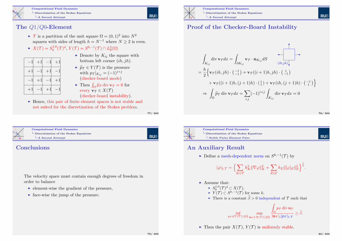
The Q1/Q0-Element
I T is a partition of the unit square Ω = (0, 1)2 into N2
squares with sides of length h = N−1 where N ≥ 2 is even.
I X(T ) = S1,00 (T )d, Y (T ) = S0,−1(T ) ∩ L2
0(Ω)
+1 +1
+1 +1
+1 +1
+1 +1
−1 −1
−1 −1
−1 −1
−1 −1
I Denote by Kij the square withbottom left corner (ih, jh).
I pT ∈ Y (T ) is the pressurewith pT |Kij = (−1)i+j
(checker-board mode)
I Then∫
Ω pT divvT = 0 forevery vT ∈ X(T )(checker-board instability).
I Hence, this pair of finite element spaces is not stable andnot suited for the discretization of the Stokes problem.
77/ 300
Computational Fluid Dynamics
Discretization of the Stokes Equations
A Second Attempt
Proof of the Checker-Board Instability
∫Kij
divvT dx =
∫∂Kij
vT · nKijdS -
?
6
(ih,jh)
=h
2
vT (ih, jh) ·
(−1−1
)+ vT ((i+ 1)h, jh) ·
(1−1
)+ vT ((i+ 1)h, (j + 1)h) · ( 1
1 ) + vT (ih, (j + 1)h) ·(−1
1
)⇒∫
ΩpT divvT dx =
∑i,j
(−1)i+j∫Kij
divvT dx = 0
78/ 300
Computational Fluid Dynamics
Discretization of the Stokes Equations
A Second Attempt
Conclusions
The velocity space must contain enough degrees of freedom inorder to balance
I element-wise the gradient of the pressure,
I face-wise the jump of the pressure.
79/ 300
Computational Fluid Dynamics
Discretization of the Stokes Equations
Stable Finite Element Pairs
An Auxiliary Result
I Define a mesh-dependent norm on Sk,−1(T ) by
|ϕ|1,T =∑K∈T
h2K‖∇ϕ‖2K +
∑E∈E
hE‖[ϕ]E‖2E 1
2.
I Assume that:I S1,0
0 (T )d ⊂ X(T ),I Y (T ) ⊂ Sk,−1(T ) for some k,I There is a constant β > 0 independent of T such that
infpT ∈Y (T )\0
supuT ∈X(T )\0
∫Ω
pT divuT
|uT |1|pT |1,T≥ β.
I Then the pair X(T ), Y (T ) is uniformly stable.
80/ 300
Computational Fluid Dynamics
Discretization of the Stokes Equations
Stable Finite Element Pairs
Proof of the Auxiliary Result. 1st StepI Choose a pressure pT ∈ Y (T ) with ‖pT ‖ = 1.I Due to the well-posedness of the Stokes problem, there is a
velocity u ∈ H10 (T )d with
|u|1 = 1 and
∫ΩpT divu ≥ β.
I RT u satisfies
|RT u|1 ≤ c1|u|1 = c1,∫ΩpT div(RT u) =
∫ΩpT divu +
∫ΩpT div(RT u− u)
≥ β +
∫ΩpT div(RT u− u).
81/ 300
Computational Fluid Dynamics
Discretization of the Stokes Equations
Stable Finite Element Pairs
Proof of the Auxiliary Result. 2nd Step
I Integration by parts and the properties of RT imply∫ΩpT div(RT u− u)
=∑K∈T
∫K∇pT · (u−RT u) +
∑E∈E
∫E
[pT ]E(RT u− u) · nE
≤ c2|pT |1,T |u|1.
I The last two estimates yield
supuT ∈X(T )\0
∫ΩpT divuT
|uT |1≥ 1
c1
β − c2|pT |1,T
.
82/ 300
Computational Fluid Dynamics
Discretization of the Stokes Equations
Stable Finite Element Pairs
Proof of the Auxiliary Result. 3rd Step
I The previous estimate and the third assumption imply
supuT ∈X(T )\0
∫ΩpT divuT
|uT |1
≥ maxβ|pT |1,T ,
1
c1
β − c2|pT |1,T
≥ min
z≥0max
βz,
1
c1
β − c2z
=
ββ
c1β + c2
.
83/ 300
Computational Fluid Dynamics
Discretization of the Stokes Equations
Stable Finite Element Pairs
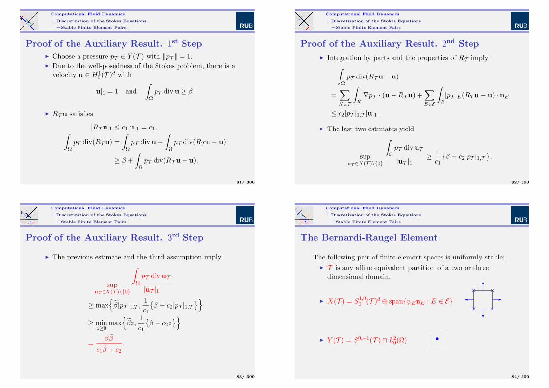
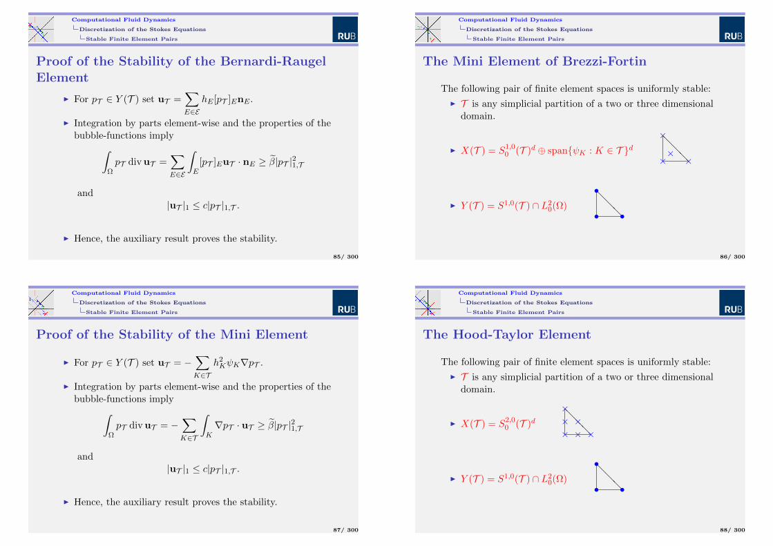
The Bernardi-Raugel Element
The following pair of finite element spaces is uniformly stable:
I T is any affine equivalent partition of a two or threedimensional domain.
I X(T ) = S1,00 (T )d ⊕ spanψEnE : E ∈ E -
?
6
× ×
××
I Y (T ) = S0,−1(T ) ∩ L20(Ω) •
84/ 300
Computational Fluid Dynamics
Discretization of the Stokes Equations
Stable Finite Element Pairs
Proof of the Stability of the Bernardi-RaugelElement
I For pT ∈ Y (T ) set uT =∑E∈E
hE [pT ]EnE .
I Integration by parts element-wise and the properties of thebubble-functions imply∫
ΩpT divuT =
∑E∈E
∫E
[pT ]EuT · nE ≥ β|pT |21,T
and|uT |1 ≤ c|pT |1,T .
I Hence, the auxiliary result proves the stability.
85/ 300
Computational Fluid Dynamics
Discretization of the Stokes Equations
Stable Finite Element Pairs
The Mini Element of Brezzi-Fortin
The following pair of finite element spaces is uniformly stable:
I T is any simplicial partition of a two or three dimensionaldomain.
I X(T ) = S1,00 (T )d ⊕ spanψK : K ∈ T d
@@@× ×
×
×
I Y (T ) = S1,0(T ) ∩ L20(Ω)
@@@• •
•
86/ 300
Computational Fluid Dynamics
Discretization of the Stokes Equations
Stable Finite Element Pairs
Proof of the Stability of the Mini Element
I For pT ∈ Y (T ) set uT = −∑K∈T
h2KψK∇pT .
I Integration by parts element-wise and the properties of thebubble-functions imply∫
ΩpT divuT = −
∑K∈T
∫K∇pT · uT ≥ β|pT |21,T
and|uT |1 ≤ c|pT |1,T .
I Hence, the auxiliary result proves the stability.
87/ 300
Computational Fluid Dynamics
Discretization of the Stokes Equations
Stable Finite Element Pairs
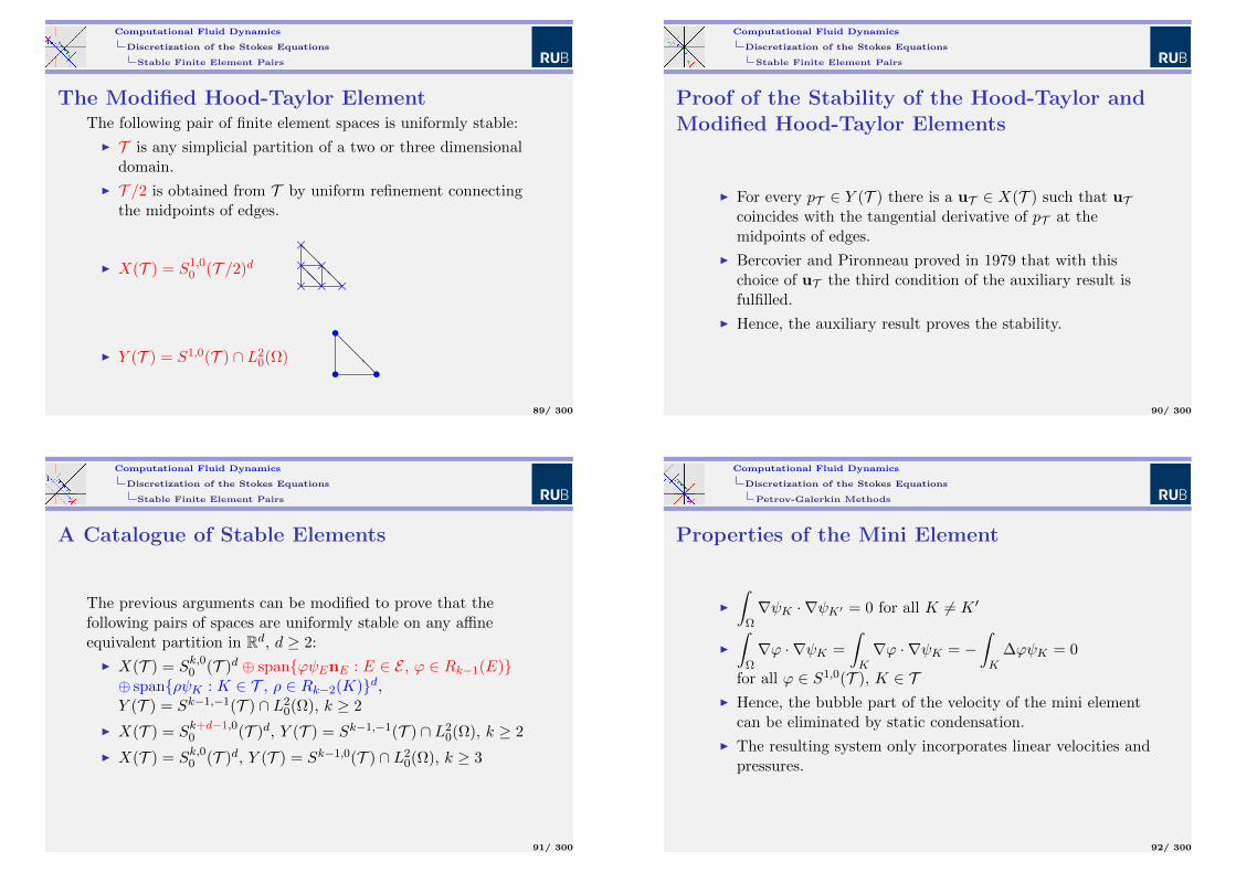
The Hood-Taylor Element
The following pair of finite element spaces is uniformly stable:
I T is any simplicial partition of a two or three dimensionaldomain.
I X(T ) = S2,00 (T )d
@@@× ×
×
×××
I Y (T ) = S1,0(T ) ∩ L20(Ω)
@@@• •
•
88/ 300
Computational Fluid Dynamics
Discretization of the Stokes Equations
Stable Finite Element Pairs
The Modified Hood-Taylor ElementThe following pair of finite element spaces is uniformly stable:
I T is any simplicial partition of a two or three dimensionaldomain.
I T /2 is obtained from T by uniform refinement connectingthe midpoints of edges.
I X(T ) = S1,00 (T /2)d
@@@@@× ×
×
×××
I Y (T ) = S1,0(T ) ∩ L20(Ω)
@@@• •
•
89/ 300
Computational Fluid Dynamics
Discretization of the Stokes Equations
Stable Finite Element Pairs
Proof of the Stability of the Hood-Taylor andModified Hood-Taylor Elements
I For every pT ∈ Y (T ) there is a uT ∈ X(T ) such that uTcoincides with the tangential derivative of pT at themidpoints of edges.
I Bercovier and Pironneau proved in 1979 that with thischoice of uT the third condition of the auxiliary result isfulfilled.
I Hence, the auxiliary result proves the stability.
90/ 300
Computational Fluid Dynamics
Discretization of the Stokes Equations
Stable Finite Element Pairs
A Catalogue of Stable Elements
The previous arguments can be modified to prove that thefollowing pairs of spaces are uniformly stable on any affineequivalent partition in Rd, d ≥ 2:
I X(T ) = Sk,00 (T )d ⊕ spanϕψEnE : E ∈ E , ϕ ∈ Rk−1(E)⊕ spanρψK : K ∈ T , ρ ∈ Rk−2(K)d,Y (T ) = Sk−1,−1(T ) ∩ L2
0(Ω), k ≥ 2
I X(T ) = Sk+d−1,00 (T )d, Y (T ) = Sk−1,−1(T ) ∩ L2
0(Ω), k ≥ 2
I X(T ) = Sk,00 (T )d, Y (T ) = Sk−1,0(T ) ∩ L20(Ω), k ≥ 3
91/ 300
Computational Fluid Dynamics
Discretization of the Stokes Equations
Petrov-Galerkin Methods
Properties of the Mini Element
I
∫Ω∇ψK · ∇ψK′ = 0 for all K 6= K ′
I
∫Ω∇ϕ · ∇ψK =
∫K∇ϕ · ∇ψK = −
∫K
∆ϕψK = 0
for all ϕ ∈ S1,0(T ), K ∈ TI Hence, the bubble part of the velocity of the mini element
can be eliminated by static condensation.
I The resulting system only incorporates linear velocities andpressures.
92/ 300
Computational Fluid Dynamics
Discretization of the Stokes Equations
Petrov-Galerkin Methods
The Mini Element with Static CondensationI Original system:A` 0 BT
`
0 Db BTb
B` Bb 0
u`ubp
=
f`fb0
I System with static condensation:(
A` BT`
B` −BbD−1b BT
b
)(u`p
)=
(f`
−BbD−1b fb
)I A straightforward calculation yields:(
BbD−1b BT
b
)i,j≈∑K∈T
h2K
∫K∇λi · ∇λj
93/ 300
Computational Fluid Dynamics
Discretization of the Stokes Equations
Petrov-Galerkin Methods
Idea of Petrov-Galerkin Methods
I Try to obtain control on the pressure by adding
I element-wise terms of the form δKh2K
∫K
∇pT · ∇qT ,
I face-wise terms of the form δEhE
∫E
[pT ]E [qT ]E .
I The form of the scaling parameters is motivated by theMini element and the request that element and facecontributions should be of comparable size.
I The resulting problem should be coercive.
I Contrary to penalty methods, the additional terms shouldbe consistent with the variational problem, i.e. they shouldvanish for the weak solution of the Stokes problem.
I Pressure-jumps are no problem.
I Test the momentum equation element-wise with δKh2K∇qT .
94/ 300
Computational Fluid Dynamics
Discretization of the Stokes Equations
Petrov-Galerkin Methods
General Form of Petrov-Galerkin Methods
Find uT ∈ X(T ), pT ∈ Y (T ) such that for all vT ∈ X(T ),qT ∈ Y (T )∫
Ω∇uT : ∇vT −
∫ΩpT divvT =
∫Ωf · vT∫
ΩqT divuT
+∑K∈T
δKh2K
∫K
(−∆uT +∇pT ) · ∇qT
+∑E∈ET
δEhE
∫E
[pT ]E [qT ]E =∑K∈T
δKh2K
∫Kf · ∇qT
95/ 300
Computational Fluid Dynamics
Discretization of the Stokes Equations
Petrov-Galerkin Methods
Choice of Stabilization Parameters
I Set
δmax = maxmaxK∈T
δK , maxE∈ET
δE,
δmin =
minmin
K∈TδK , min
E∈ETδE if pressures
are discontinuous,
minK∈T
δK if pressures
are continuous.
I A reasonable choice of the stabilization parameters then isdetermined by the condition
δmax ≈ δmin.
96/ 300
Computational Fluid Dynamics
Discretization of the Stokes Equations
Petrov-Galerkin Methods
Choice of Spaces
I Optimal with respect to error estimates versus degrees offreedom:
X(T ) = Sk,00 (T )d
Y (T ) =
Sk−1,0(T ) ∩ L2
0(Ω) continuous pressure
Sk−1,−1(T ) ∩ L20(Ω) discontinuous pressure
I Equal order interpolation:
X(T ) = Sk,00 (T )d
Y (T ) =
Sk,0(T ) ∩ L2
0(Ω) continuous pressure
Sk,−1(T ) ∩ L20(Ω) discontinuous pressure
97/ 300
Computational Fluid Dynamics
Discretization of the Stokes Equations
Petrov-Galerkin Methods
Mesh-Dependent Norms and (Bi-)Linear Forms
I ‖|(uT , pT )‖|1,T =|uT |21 + ‖pT ‖2 + |pT |21,T
12
I BT ((uT , pT ), (vT , qT ))
=
∫Ω∇uT : ∇vT −
∫ΩpT divvT +
∫ΩqT divuT
+∑K∈T
δKh2K
∫K
(−∆uT +∇pT ) · ∇qT
+∑E∈E
δEhE
∫E
[pT ]E [qT ]E
I `T ((vT , qT )) =
∫Ωf · vT +
∑K∈T
δKh2K
∫Kf · ∇qT
98/ 300
Computational Fluid Dynamics
Discretization of the Stokes Equations
Petrov-Galerkin Methods
Stability of the Petrov-Galerkin Discretization
I Assume that δmin > 0 and δmax < δ0 where δ0 only dependson the shape parameter of T .
I Then there is a constant γ > 0 which does not depend onT such that
inf(uT ,pT )
sup(vT ,qT )
BT ((uT , pT ), (vT , qT ))
‖|(uT , pT )‖|1,T ‖|(vT , qT )‖|1,T≥ γ.
99/ 300
Computational Fluid Dynamics
Discretization of the Stokes Equations
Petrov-Galerkin Methods
Proof of the Stability
I Inverse estimates imply that
BT ((uT , pT ), (uT , pT )) ≥ 1
2δmin
‖|(uT , pT )‖|21,T − ‖pT ‖2
I Due to the well-posedness of the Stokes problem, there is a
velocity v ∈ H10 (T )d with |v|1 = ‖pT ‖ and∫
ΩpT divv ≥ β‖pT ‖2.
I The properties of RT imply that
BT ((uT , pT ), (RT v, 0)) ≥(1
4+ β2
)‖pT ‖2 − β2‖|(uT , pT )‖|21,T ,
‖|(RT v, 0)‖|1,T ≤ cΩ‖pT ‖.
I Taking the maximum of both estimates proves the stability.
100/ 300
Computational Fluid Dynamics
Discretization of the Stokes Equations
Petrov-Galerkin Methods
Error Estimates
I There is a constant c ≈ δmaxγ−1 such that
‖|(u− uT , p− pT )‖|1,T
≤ c inf(vT ,qT )
‖|(u− vT , p− qT )‖|21,T
+∑K∈T
h2K‖∆(u− vT )‖2K
12.
I If u ∈ Hk+1(Ω)d ∩H10 (Ω)d, p ∈ Hk(Ω) ∩ L2
0(Ω),
Sk,00 (T )d ⊂ X(T ) and Sk−1,−1(T ) ∩ L20(Ω) ⊂ Y (T ) or
Sk−1,0(T ) ∩ L20(Ω) ⊂ Y (T ) then
‖|(u− uT , p− pT )‖|1,T ≤ c′hk|u|k+1 + |p|k
.
101/ 300
Computational Fluid Dynamics
Discretization of the Stokes Equations
Petrov-Galerkin Methods
Proof of the Error EstimatesThe stability and the definitions of BT and `T yield
I ‖|(u− uT , p− pT )‖|1,T≤ ‖|(u− vT , p− qT )‖|1,T + ‖|(vT − uT , qT − pT )‖|1,T
I ‖|(vT − uT , qT − pT )‖|1,T
≤ 1
γsup
(wT ,rT )
BT ((vT − uT , qT − pT ), (wT , rT ))
‖|(wT , rT )‖|1,TI BT ((vT − uT , qT − pT ), (wT , rT ))
= BT ((vT − u, qT − p), (wT , rT ))
≤ c′′‖|(u− vT , p− qT )‖|21,T +
∑K∈T
h2K‖∆(u− vT )‖2K
12 ·
‖|(wT , rT )‖|1,T
102/ 300
Computational Fluid Dynamics
Discretization of the Stokes Equations
Non-Conforming Discretizations
The Basic Idea
I We want a fully conservative discretization, i.e. the discretesolution has to satisfy divuT = 0.
I As a trade-off, we are willing to relax the conformitycondition X(T ) ⊂ H1
0 (Ω)d.
103/ 300
Computational Fluid Dynamics
Discretization of the Stokes Equations
Non-Conforming Discretizations
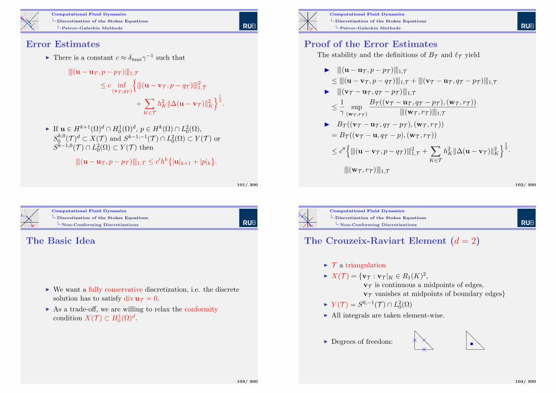
The Crouzeix-Raviart Element (d = 2)
I T a triangulation
I X(T ) = vT : vT |K ∈ R1(K)2,vT is continuous a midpoints of edges,vT vanishes at midpoints of boundary edges
I Y (T ) = S0,−1(T ) ∩ L20(Ω)
I All integrals are taken element-wise.
I Degrees of freedom:@@@××× @
@@
•
104/ 300

Computational Fluid Dynamics
Discretization of the Stokes Equations
Non-Conforming Discretizations
Properties of the Crouzeix-Raviart Element
I The Crouzeix-Raviart discretization admits a uniquesolution uT , pT .
I The discretization is fully conservative, i.e. the continuityequation divuT = 0 is satisfied element-wise.
I If Ω is convex, the following error estimates hold∑K∈T|u− uT |21,K
12
+ ‖p− pT ‖ ≤ ch‖f‖,
‖u− uT ‖ ≤ ch2‖f‖.
105/ 300
Computational Fluid Dynamics
Discretization of the Stokes Equations
Non-Conforming Discretizations
Drawbacks of the Crouzeix-Raviart Element
I Its accuracy deteriorates drastically in the presence ofre-entrant corners.
I It has no higher order equivalent.
I It has no three-dimensional equivalent.
106/ 300
Computational Fluid Dynamics
Discretization of the Stokes Equations
Non-Conforming Discretizations
Construction of a Solenoidal Bases
I Denote by ϕE ∈ S1,−1(T ) the function which takes thevalue 1 at the midpoint of E and vanishes at all othermidpoints of edges.
I Set wE = ϕEtE where tE is a unit vector tangential to E.
I Set wx =∑E∈Ex
1
|E|ϕEnE,x. @
@@
@@@@@@
@@@6
? -
I Then
V (T ) =uT ∈ X(T ) : divuT = 0
= span
wx,wE : x ∈ NΩ, E ∈ EΩ
107/ 300
Computational Fluid Dynamics
Discretization of the Stokes Equations
Non-Conforming Discretizations
Solution of the Discrete Problem
I The velocity uT ∈ V (T ) is determined by the conditions∑K∈T
∫K∇uT : ∇vT =
∑K∈T
∫Kf · vT
for all vT ∈ V (T ).
I The pressure pT is determined by the conditions∑K∈T
∫Kf · nEϕE −
∑K∈T
∫K∇uT : (∇ϕE ⊗ nE) = −|E|[pT ]E
for all E ∈ EΩ.
108/ 300
Computational Fluid Dynamics
Discretization of the Stokes Equations
Non-Conforming Discretizations
Computation of the Velocity
The problem for the velocity
I is symmetric positive definite,
I corresponds to a Morley element discretization of thebiharmonic equation,
I has condition number O(h−4).
109/ 300
Computational Fluid Dynamics
Discretization of the Stokes Equations
Non-Conforming Discretizations
Computation of the Pressure
I Set F = ∅, M = ∅.I Choose an element K ∈ T with an edge on the boundary.
I Set pT = 0 on K.I Add K to M.
I While M 6= ∅ do:I Choose an element K ∈M.I For all elements K ′ which share an edge with K and which
are not contained in F do:I On K′ set pT equal to the value of pT on K plus the jump
across the common edge.I If K′ is not contained in M, add it to M.
I Remove K from M and add it to F .
I Compute the average of pT and subtract it from pT onevery element.
110/ 300
Computational Fluid Dynamics
Discretization of the Stokes Equations
Stream-Function Formulation
The curl Operators (d = 2)
I curlϕ =
(− ∂ϕ∂x2∂ϕ∂x1
)I curlv = ∂v1
∂x2− ∂v2
∂x1
I curl(curlϕ) = −∆ϕ
I curl(curlv) = −∆v +∇(divv)
I curl(∇ϕ) = 0
I divu = 0 if and only if there is a stream-function ψ withψ = 0 on Γ and u = curlψ in Ω
111/ 300
Computational Fluid Dynamics
Discretization of the Stokes Equations
Stream-Function Formulation
Stream-Function Formulation of theTwo-Dimensional Stokes Equations
Taking the curl of the momentum equation proves:
I u is a solution of the two-dimensional Stokes equations ifand only if
I u = curlψ and ψ solves the biharmonic equation
∆2ψ = curl f in Ω
ψ = 0 on Γ
∂ψ
∂n= 0 on Γ
112/ 300
Computational Fluid Dynamics
Discretization of the Stokes Equations
Stream-Function Formulation
Drawbacks of the Stream-Function Formulation
I It is restricted to two dimensions.
I It gives no information on the pressure.
I A conforming discretization of the biharmonic equationrequires C1-elements.
I Low order non-conforming discretizations of thebiharmonic equation are equivalent to the Crouzeix-Raviartdiscretization.
I Mixed formulations of the biharmonic equation using thevorticity ω = curlu as additional variable are at least asdifficult to discretize as the original Stokes problem.
113/ 300
Computational Fluid Dynamics
Solution of the Discrete Problems
Solution of the Discrete Problems
I Motivation
I Uzawa Type Algorithms
I Multigrid Algorithms
I Subspace Decomposition Methods
I Conjugate Gradient Type Algorithms
114/ 300
Computational Fluid Dynamics
Solution of the Discrete Problems
Motivation
Direct Solvers
I Typically require O(N2− 1d ) storage for a discrete problem
with N unknowns.
I Typically require O(N3− 2d ) operations.
I Yield the exact solution of the discrete problem up torounding errors.
I Yield an approximation for the differential equation withan O(hα) = O(N−
αd ) error (typically: α ∈ 1, 2).
115/ 300
Computational Fluid Dynamics
Solution of the Discrete Problems
Motivation
Iterative Solvers
I Typically require O(N) storage.
I Typically require O(N) operations per iteration.
I Their convergence rate deteriorates with an increasingcondition number of the discrete problem which typically isO(h−2) = O(N
2d ).
I In order to reduce an initial error by a factor 0.1 onetypically needs the following numbers of operations:
I O(N1+ 2d ) with the Gauß-Seidel algorithm,
I O(N1+ 1d ) with the conjugate gradient (CG-) algorithm,
I O(N1+ 12d ) with the CG-algorithm with Gauß-Seidel
preconditioning,I O(N) with a multigrid (MG-) algorithm.
116/ 300
Computational Fluid Dynamics
Solution of the Discrete Problems
Motivation
Nested Grids
I Often one has to solve a sequence of discrete problemsLkuk = fk corresponding to increasingly more accuratediscretizations.
I Typically there is a natural interpolation operator Ik−1,k
which maps functions associated with the (k − 1)-stdiscrete problem into those corresponding to the k-thdiscrete problem.
I Then the interpolate of any reasonable approximatesolution of the (k − 1)-st discrete problem is a good initialguess for any iterative solver applied to the k-th discreteproblem.
I Often it suffices to reduce the initial error by a factor 0.1.
117/ 300
Computational Fluid Dynamics
Solution of the Discrete Problems
Motivation
Nested Iteration
I Computeu0 = u0 = L−1
0 f0.
I For k = 1, . . . compute an approximate solution uk foruk = L−1
k fk by applying mk iterations of an iterative solverfor the problem
Lkuk = fk
with starting value Ik−1,kuk−1.
I mk is implicitly determined by the stopping criterion
‖fk − Lkuk‖ ≤ ε‖fk − Lk(Ik−1,kuk−1)‖.
118/ 300
Computational Fluid Dynamics
Solution of the Discrete Problems
Uzawa Type Algorithms
Structure of Discrete Stokes Problems
Discrete Stokes problems have the form(
A BBT −δC
)( up ) =
(fδg
)with:
I δ = 0 for mixed methods,
I 0 < δ ≈ 1 for Petrov-Galerkin methods,
I a square, symmetric, positive definite nu × nu matrix Awith condition of O(h−2),
I a rectangular nu × np matrix B,
I a square, symmetric, positive definite np × np matrix Cwith condition of O(1),
I a vector f of dimension nu discretizing the exterior force,
I a vector g of dimension np which equals 0 for mixedmethods.
119/ 300
Computational Fluid Dynamics
Solution of the Discrete Problems
Uzawa Type Algorithms
Consequences
I The stiffness matrix(
A BBT −δC
)is symmetric but indefinite,
i.e. it has positive and negative real eigenvalues.
I Hence, standard iterative methods such as the Gauß-Seideland CG-algorithms fail.
120/ 300
Computational Fluid Dynamics
Solution of the Discrete Problems
Uzawa Type Algorithms
The Uzawa Algorithm0. Given: an initial guess p0, a tolerance ε > 0 and a
relaxation parameter ω > 0.
1. Set i = 0.
2. Apply a few Gauß-Seidel iterations to the linear system
Au = f −Bpiand denote the result by ui+1. Compute
pi+1 = pi + ωBTui+1 − δg − δCpi.
3. If
‖Aui+1 +Bpi+1 − f‖+ ‖BTui+1 − δCpi+1 − δg‖ ≤ ε
return ui+1 and pi+1 as approximate solution; stop.Otherwise increase i by 1 and go to step 2.
121/ 300
Computational Fluid Dynamics
Solution of the Discrete Problems
Uzawa Type Algorithms
Properties of the Uzawa Algorithm
I ω ∈ (1, 2), typically ω = 1.5.
I Typically ‖v‖ =√
1nu
v · v and ‖q‖ =√
1npq · q.
I The problem Au = f −Bpi is a discrete version of dPoisson equations for the components of the velocity field.
I The Uzawa algorithm falls into the class of pressurecorrection schemes.
I The convergence rate of the Uzawa algorithm is 1−O(h2).
122/ 300
Computational Fluid Dynamics
Solution of the Discrete Problems
Uzawa Type Algorithms
Idea for an Improvement of the UzawaAlgorithm
I The problem(
A BBT −δC
)( up ) =
(fδg
)is equivalent to
u = A−1(f −Bp) and BTA−1(f −Bp)− δCp = δg.
I The matrix BTA−1B + δC is symmetric, positive definiteand has a condition of O(1).
I Hence, a standard CG-algorithm can be applied to thepressure problem and has a uniform convergence rateindependently of any mesh-size.
I The evaluation of A−1g corresponds to the solution of ddiscrete Poisson equations Au = g for the components of u.
I The discrete Poisson problems can efficiently be solvedwith a MG-algorithm.
123/ 300
Computational Fluid Dynamics
Solution of the Discrete Problems
Uzawa Type Algorithms
Properties of BTA−1B
I Identify vectors with corresponding finite elementfunctions.
I u = A−1Bp satisfies:
I
∫Ω
∇u : ∇v =
∫Ω
p divv for all v,
I |u|1 ≤√d‖p‖,
I |u|1 ≥ β‖p‖ (inf-sup condition).
I q = BTu = BTA−1Bp satisfies:
I
∫Ω
qr =
∫Ω
r divu for all r,
I ‖q‖ ≤√d|u|1 ≤ d‖p‖,
I β2‖p‖2 ≤ |u|21 =
∫Ω
p divu =
∫Ω
qp ≤ ‖q‖‖p‖.
124/ 300
Computational Fluid Dynamics
Solution of the Discrete Problems
Uzawa Type Algorithms
The Improved Uzawa Algorithm
0. Given: an initial guess p0 and a tolerance ε > 0.
1. Apply a MG-algorithm with starting value zero andtolerance ε to Av = f −Bp0 and denote the result by u0.Compute r0 = BTu0 − δg − δCp0, d0 = r0, γ0 = r0 · r0. Setu0 = 0 and i = 0.
2. If γi < ε2 compute p = p0 + pi, apply a MG-algorithm withstarting value zero and tolerance ε to Av = f −Bp anddenote the result by u, stop.
3. Apply a MG-algorithm with starting value ui and toleranceε to Av = Bdi and denote the result by ui+1. Computesi = BTui+1 + δCdi, αi = γi
di·si , pi+1 = pi + αidi,
ri+1 = ri − αisi, γi+1 = ri+1 · ri+1, βi = γi+1
γi,
di+1 = ri+1 + βidi. Increase i by 1 and go to step 2.
125/ 300
Computational Fluid Dynamics
Solution of the Discrete Problems
Uzawa Type Algorithms
Properties of the Improved Uzawa Algorithm
I It is a nested iteration with MG-iterations in the innerloops.
I Typically 2 to 4 MG-iterations suffice in the inner loops.
I It requires O(N) operations per iteration.
I Its convergence rate is uniformly less than 1 for all meshes.
I It yields an approximate solution with error less than εwith O(N ln ε) operations.
I Numerical experiments yield convergence rates less than0.5.
126/ 300
Computational Fluid Dynamics
Solution of the Discrete Problems
Uzawa Type Algorithms
Convergence Rate of the Improved UzawaAlgorithm
I Denote by Mv the result of the MG-algorithm applied to aproblem with right-hand side v.
I The improved Uzawa algorithm then corresponds to aCG-algorithm applied to the problemBTM(f −Bp)− δCp = δg.
I Properties of the MG-algorithm imply thatI M is symmetric,I M satisfies ‖Mv −A−1v‖ ≤ ε‖A−1v‖ for all v.
I Hence,(1− ε)pTBTA−1Bp ≤ pTBTMBp ≤ (1 + ε)pTBTA−1Bpfor all p.
I Thus, BTMB is symmetric, positive definite and has acondition of O(1) uniformly for all meshes.
127/ 300
Computational Fluid Dynamics
Solution of the Discrete Problems
Multigrid Algorithms
The Basic Idea
I Classical iterative methods such as the Gauß-Seidelalgorithm quickly reduce highly oscillatory errorcomponents.
I Classical iterative methods such as the Gauß-Seidelalgorithm are very poor in reducing slowly oscillatory errorcomponents.
I Slowly oscillating error components can well be resolved oncoarser meshes with fewer unknowns.
128/ 300
Computational Fluid Dynamics
Solution of the Discrete Problems
Multigrid Algorithms
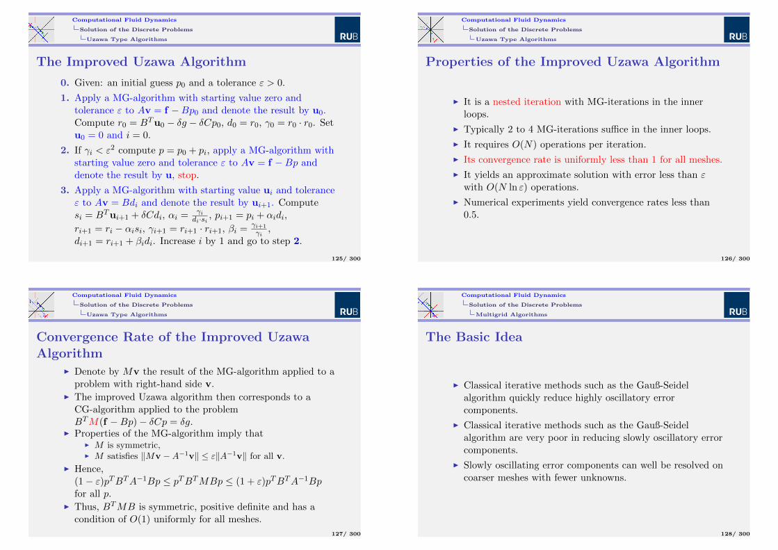
The Basic Two-Grid Algorithm
I Perform several steps of a classical iterative method on thecurrent grid.
I Correct the current approximation as follows:I Compute the current residual.I Restrict the residual to the next coarser grid.I Exactly solve the resulting problem on the coarse grid.I Prolongate the coarse-grid solution to the next finer grid.
I Perform several steps of a classical iterative method on thecurrent grid.
129/ 300
Computational Fluid Dynamics
Solution of the Discrete Problems
Multigrid Algorithms
Schematic Form
Two-Grid
G−−−−→ G−−−−→
Ry xP
E−−−−→
Multigrid
G−−−−→ G−−−−→
Ry xP
G−−−−→ G−−−−→
Ry xP
E−−−−→
130/ 300
Computational Fluid Dynamics
Solution of the Discrete Problems
Multigrid Algorithms
Basic Ingredients
I A sequence Tk of increasingly refined meshes withassociated discrete problems Lkuk = fk.
I A smoothing operator Mk, which should be easy toevaluate and which at the same time should give areasonable approximation to L−1
k .
I A restriction operator Rk,k−1, which maps functions on afine mesh Tk to the next coarser mesh Tk−1.
I A prolongation operator Ik−1,k, which maps functions froma coarse mesh Tk−1 to the next finer mesh Tk.
131/ 300
Computational Fluid Dynamics
Solution of the Discrete Problems
Multigrid Algorithms
The Multigrid Algorithm
0. Given: the actual level k, parameters µ, ν1, and ν2, thematrix Lk, the right-hand side fk, an initial guess uk.Sought: improved approximate solution uk.
1. If k = 0 compute u0 = L−10 f0; stop.
2. (Pre-smoothing) Perform ν1 steps of the iterativeprocedure uk 7→ uk +Mk(fk − Lkuk).
3. (Coarse grid correction)3.1 Compute fk−1 = Rk,k−1(fk − Lkuk) and set uk−1 = 0.3.2 Perform µ iterations of the MG-algorithm with parameters
k − 1, µ, ν1, ν2, Lk−1, fk−1, uk−1 and denote the result byuk−1.
3.3 Update uk by uk 7→ uk + Ik−1,kuk−1.
4. (Post-smoothing) Perform ν2 steps of the iterativeprocedure uk 7→ uk +Mk(fk − Lkuk).
132/ 300
Computational Fluid Dynamics
Solution of the Discrete Problems
Multigrid Algorithms
Typical Choices of Parameters
I µ = 1 V-cycle or
µ = 2 W-cycle
I ν1 = ν2 = ν or
ν1 = ν, ν2 = 0 or
ν1 = 0, ν2 = ν
I 1 ≤ ν ≤ 4.
133/ 300
Computational Fluid Dynamics
Solution of the Discrete Problems
Multigrid Algorithms
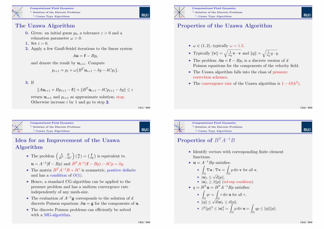
Prolongation and Restriction
I The prolongation is typically determined by the naturalinclusion of the finite element spaces, i.e. a finite elementfunction corresponding to a coarse mesh is expressed interms of the finite element bases functions corresponding tothe fine mesh.
@@@
1 0
0
@@
12
12
0
@@@
1 0
0
12
I The restriction is typically determined by inserting finiteelement bases functions corresponding to the coarse meshin the variational form of the discrete problemcorresponding to the fine mesh.
134/ 300
Computational Fluid Dynamics
Solution of the Discrete Problems
Multigrid Algorithms
Smoothing (Positive Definite Problems)
I Gauß-Seidel iteration
I SSOR iteration:I Perform a forward Gauß-Seidel sweep with over-relaxation
as pre-smoothing.I Perform a backward Gauß-Seidel sweep with over-relaxation
as post-smoothing.
I ILU smoothing:I Perform an incomplete lower upper decomposition of Lk by
suppressing all fill-in.I The result is an approximate decomposition LkUk ≈ Lk.I Compute vk = Mkuk by solving the system LkUkvk = uk.
135/ 300
Computational Fluid Dynamics
Solution of the Discrete Problems
Multigrid Algorithms
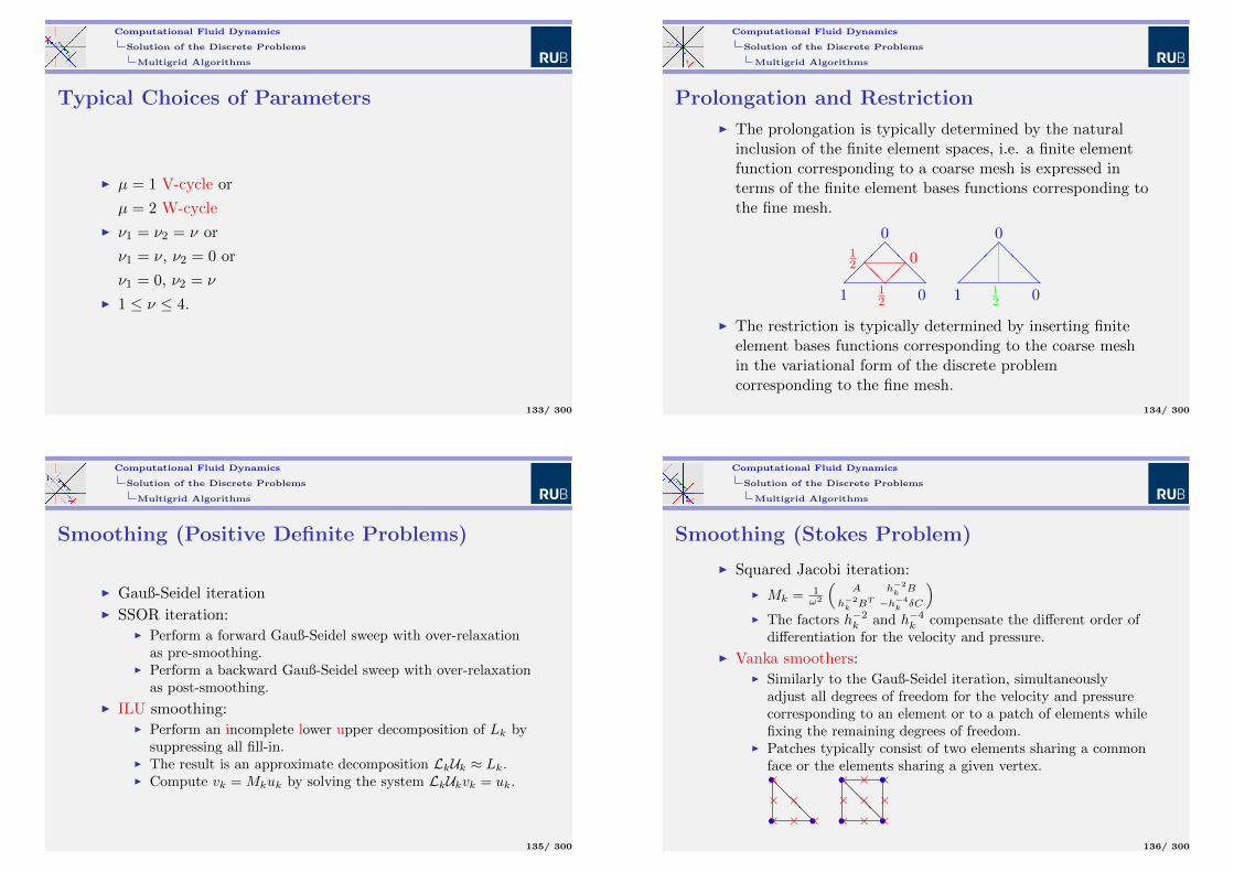
Smoothing (Stokes Problem)
I Squared Jacobi iteration:
I Mk = 1ω2
(A h−2
k B
h−2k BT −h−4
k δC
)I The factors h−2
k and h−4k compensate the different order of
differentiation for the velocity and pressure.
I Vanka smoothers:I Similarly to the Gauß-Seidel iteration, simultaneously
adjust all degrees of freedom for the velocity and pressurecorresponding to an element or to a patch of elements whilefixing the remaining degrees of freedom.
I Patches typically consist of two elements sharing a commonface or the elements sharing a given vertex.
@@@• •
•
× ×
××××
@@@• •
• •
× ×
×××××××
136/ 300
Computational Fluid Dynamics
Solution of the Discrete Problems
Multigrid Algorithms
Number of Operations
I Assume thatI one smoothing step requires O(Nk) operations,I the prolongation requires O(Nk) operations,I the restriction requires O(Nk) operations,I µ ≤ 2,I Nk > µNk−1,
I then one iteration of the multigrid algorithm requiresO(Nk) operations.
137/ 300
Computational Fluid Dynamics
Solution of the Discrete Problems
Multigrid Algorithms
Convergence Rate (Positive Definite Problems)
I The convergence rate is uniformly less than 1 for allmeshes.
I The convergence rate is bounded by cc+ν1+ν2
with aconstant which only depends on the shape parameter of themeshes.
I Numerical experiments yield convergence rates less than0.1.
138/ 300
Computational Fluid Dynamics
Solution of the Discrete Problems
Multigrid Algorithms
Convergence Rate (Stokes Problem)
I The convergence rate is uniformly less than 1 for allmeshes.
I The convergence rate is bounded by c√ν1+ν2
with a constant
which only depends on the shape parameter of the meshes.
I Numerical experiments yield convergence rates less than0.5.
139/ 300
Computational Fluid Dynamics
Solution of the Discrete Problems
Multigrid Algorithms
Techniques for Proving the Convergence ofMultigrid Algorithms
I Methods of linear algebra and discrete Fourier analysis(Hackbusch)
I Spectral decomposition and scales of discrete Sobolevspaces (Bank-DuPont and Braess-Hackbusch)
I Subspace decomposition methods (Bramble-Pasciak-Xuand Wang)
140/ 300
Computational Fluid Dynamics
Solution of the Discrete Problems
Multigrid Algorithms
Convergence Proof a la Hackbusch
I The iteration matrix of the smoother is Nk = I −MkLk.
I The iteration matrix of the two-grid algorithm isSk = Nν2
k (I − Ik−1,kL−1k−1Rk,k−1)Nν1
k .
I The iteration matrix of the multigrid algorithm isSk = Sk +Nν2
k Ik−1,kSµk−1L
−1k−1Rk,k−1N
ν1k .
I Prove the smoothing property LkNνk ≤ η(ν)h−αk with
η(ν)→ 0 for ν →∞ and α ≥ 0.
I Prove the approximation property‖|L−1
k − Ik−1,kL−1k−1Rk,k−1‖| ≤ chα.
I The smoothing and approximation property imply‖|Sk‖| ≤ cη(ν1 + ν2).
I If µ ≥ 2 a perturbation argument yields‖|Sk‖| ≤ 2cη(ν1 + ν2).
141/ 300
Computational Fluid Dynamics
Solution of the Discrete Problems
Multigrid Algorithms
Establishing the Smoothing and ApproximationProperty
I The proof of the smoothing property is usually based on aspectral decomposition of Lk and Nk.
I The proof of the approximation property is usually basedon arguments used in the proof of a priori error estimates.
I The crucial point is to correctly link both techniques.
142/ 300
Computational Fluid Dynamics
Solution of the Discrete Problems
Multigrid Algorithms
Convergence Proof a la Braess-Hackbusch
I Assume that Lk is symmetric, positive definite and set‖|vk‖| = (vk, Lkvk)
12 .
I Denote by Qk = Ik−1,kL−1k−1Rk,k−1Lk the Ritz projection.
I Denote by Jk the iteration matrix of the Jacobi iteration
and set |vk| = ‖|J12k vk‖| and ρ(vk) = |vk|2
‖|vk‖|2.
I Prove thatI ‖|Jνk vk‖| ≤ ρν‖|vk‖| with ρ = ρ(Jνk vk),I ‖|vk −Qkvk‖| ≤ min1, c
√1− ρ(vk)‖|vk‖|.
I Then the convergence rate δk of the multigrid algorithmwith µ = 1 and ν1 = ν2 = ν and Jacobi smoothing satisfies
δk ≤ max0≤ρ≤1
ρ2ν[δk−1 + (1− δk−1) min1, c(1− ρ)
].
I By induction this proves δk ≤ cc+2ν .
143/ 300
Computational Fluid Dynamics
Solution of the Discrete Problems
Subspace Decomposition Methods
The Setting
I V a finite dimensional Hilbert space with inner product(·, ·)
I Vi, 1 ≤ i ≤ N , subspaces of V with∑
i Vi = V
The decomposition usually neither is direct nor orthogonal.
I Qi : V → Vi orthogonal projection w.r.t. to (·, ·)I A : v → V a symmetric, positive definite operator
I Ai : Vi → Vi the restriction of A to Vi
I Ri : Vi → Vi an easy-to-evaluate, symmetric, positivedefinite approximation to A−1
i
144/ 300
Computational Fluid Dynamics
Solution of the Discrete Problems
Subspace Decomposition Methods
The Subspace Decomposition Algorithm
I Given an initial guess u0 ∈ V .
I For n = 0, 1, . . . and j = 1, . . . , N compute
un+ jN
= un+ j−1N
+RjQj(f −Aun+ j−1N
).
145/ 300
Computational Fluid Dynamics
Solution of the Discrete Problems
Subspace Decomposition Methods
Examples
I V = RN and Vi = spanei corresponds to the classicalGauß-Seidel algorithm.
I V = Sk,00 (TN ), Vi = Sk,00 (Ti), R0 = A−10 and Ri = 1
ωiI with
uniformly or locally refined nested meshes Ti correspondsto the multigrid algorithm with Jacobi smoothing andν1 = 1, ν2 = 0.
146/ 300
Computational Fluid Dynamics
Solution of the Discrete Problems
Subspace Decomposition Methods
Convergence Rate
I Set ‖|v‖| = (Av, v)12 .
I Set λ = mini λmax(RiAi) and Λ = maxi λmax(RiAi).
I Assume that Λ < 2.
I Assume that there are two constants K0 and K1 such that
I
N∑i=1
‖|vi‖|2 1
2 ≤ K0‖|v‖| for all v =∑i vi,
I∑
1≤i,j≤N
(Avi, wj) ≤ K1
N∑i=1
‖|vi‖|2 1
2 N∑j=1
‖|wj‖|2 1
2
for all vi ∈ Vi, wj ∈ Vj .I Then the convergence rate of the subspace decomposition
algorithm w.r.t. ‖|·‖| is less than[1−
(2Λ − 1
)(λ
ΛK0K1
)2] 12.
147/ 300
Computational Fluid Dynamics
Solution of the Discrete Problems
Subspace Decomposition Methods
Proof of the Bound for the Convergence Rate
I Set Ti = RiQiA, E0 = I, Ej = (I − Tj) · . . . · (I − T1).
I For every j this gives −Ej + Ej−1 = TjEj−1 and
‖|Ej−1v‖|2 − ‖|Ejv‖|2 = (ATjEj−1v, (2I − Tj)Ej−1v) ≥(2− Λ)(ATjEj−1v,Ej−1v).
I Summation yields‖|v‖|2 − ‖|ENv‖|2 ≥ (2− Λ)
∑j(ATjEj−1v,Ej−1v).
I The first assumption yields for v =∑
i vi
‖|v‖|2 =∑
i(A(RiAi)−1Tiv, v) ≤ λ−1K0‖|v‖|
∑i‖|Tiv‖|2
12.
I The second assumption implies∑i‖|Tiv‖|2 ≤ Λ3K2
1
∑j(ATjEj−1v,Ej−1v).
I Combining all estimates yields the bound for theconvergence rate.
148/ 300
Computational Fluid Dynamics
Solution of the Discrete Problems
Subspace Decomposition Methods
Verification of the AssumptionsI The condition Λ < 2 can be satisfied by a suitable scaling
of Ri.I Since V =
∑i Vi the mapping
V1 × . . .× VN 3 (v1, . . . , vN ) 7→∑
i vi ∈ V is surjective. Theopen mapping theorem therefore proves the firstassumption. The crucial point is to obtain an explicitbound for K0 which does not depend on N . This requiresdeep results concerning the characterization of Sobolevspaces as approximation spaces.
I Due to the Cauchy-Schwarz inequality, the secondassumption is always satisfied with K1 ≤ N . If thesubspaces satisfy a strengthened Cauchy-Schwarzinequality (Avi, wj) ≤ γ|i−j|‖|vi‖|‖|wj‖| with γ < 1, thesecond assumption is satisfied with K1 ≤ 1
1−γ .
149/ 300
Computational Fluid Dynamics
Solution of the Discrete Problems
Conjugate Gradient Type Algorithms
CG-Type Algorithms for Non-Symmetric andIndefinite Systems of Equations
I The classical CG-algorithm breaks down for non-symmetricor indefinite systems of equations.
I A naive remedy is to apply the CG-algorithm to the systemLTLu = LT f of the normal equations.
I This approach cannot be recommended since passing to thenormal system squares the condition number.
I The following variants of the CG-algorithm are particularlyadapted to non-symmetric and indefinite problems:
I the stabilized bi-conjugate gradient algorithm (Bi-CG-stabin short),
I the generalized minimal residual method (GMRES in short).
150/ 300
Computational Fluid Dynamics
Solution of the Discrete Problems
Conjugate Gradient Type Algorithms
The Idea of the Bi-CG-stab Algorithm
I The algorithm tries to simultaneously solve the originalproblem Lu = f and its adjoint problem LT v = f .
I For both problems it performs a simultaneous three-termrecursion similar to the CG-iteration.
I It incorporates particular devices to detect possiblebreak-downs and to restart the iteration before breakingdown.
I It can be combined with preconditioning. Possible methodsfor preconditioning are:
I the SSOR-iteration applied to the symmetric part of L,I incomplete factorizations of L as used in the context of
ILU-smoothing.
151/ 300
Computational Fluid Dynamics
Solution of the Discrete Problems
Conjugate Gradient Type Algorithms
The Idea of the GMRES Algorithm
I It performs a three-term recursion to build increasinglylarger Krylov spaces Kn = spanu, Lu, . . . , Ln−1u.
I For every Krylov space Kn it approximately solves theminimization problem vn = argminw∈Kn‖Lw − f‖ using aQR-method.
152/ 300
Computational Fluid Dynamics
A Posteriori Error Estimation and Adaptivity
A Posteriori Error Estimation and Adaptivity
I Motivation
I A Posteriori Error Estimates for the Stokes Problem
I Mesh Refinement, Coarsening and Smoothing
153/ 300
Computational Fluid Dynamics
A Posteriori Error Estimation and Adaptivity
Motivation
Drawbacks of A Priori Error Estimates
I They only yield information on the asymptotic behaviourof the error.
I They require regularity properties of the solution whichoften are not realistic.
I They give no information on the actual size of the error.
I They are not able to detect local singularities arising fromre-entrant corners or boundary or interior layers whichdeteriorate the overall accuracy of the discretization.
154/ 300
Computational Fluid Dynamics
A Posteriori Error Estimation and Adaptivity
Motivation
Goal of A Posteriori Error Estimation andAdaptivity
I We want to obtain explicit information about the error ofthe discretization and its spatial (and temporal)distribution.
I The information should a posteriori be extracted from thecomputed numerical solution and the given data of theproblem.
I The cost for obtaining this information should be far lessthan for the computation of the numerical solution.
I We want to obtain a numerical solution with a prescribedtolerance using a (nearly) minimal number of grid-points.
I To this end we need reliable upper and lower bounds forthe true error in a user-specified norm.
155/ 300
Computational Fluid Dynamics
A Posteriori Error Estimation and Adaptivity
Motivation
General Adaptive Algorithm
0. Given: The data of a partial differential equation and atolerance ε.Sought: A numerical solution with an error less than ε.
1. Construct an initial coarse mesh T0 representing sufficientlywell the geometry and data of the problem; set k = 0.
2. Solve the discrete problem on Tk.3. For every element K in Tk compute an a posteriori error
indicator.
4. If the estimated global error is less than ε then stop.Otherwise decide which elements have to be refined orcoarsened and construct the next mesh Tk+1. Replace k byk + 1 and return to step 2.
156/ 300
Computational Fluid Dynamics
A Posteriori Error Estimation and Adaptivity
Motivation
Basic Ingredients
I An error indicator which furnishes the a posteriori errorestimate.
I A refinement strategy which determines which elementshave to be refined or coarsened and how this has to bedone.
157/ 300
Computational Fluid Dynamics
A Posteriori Error Estimation and Adaptivity
A Posteriori Error Estimates for the Stokes Problem
The Stokes Problem and its Discretization
I u ∈ H10 (Ω)d, p ∈ L2
0(Ω) weak solution of the Stokesproblem with no-slip boundary condition:
−∆u + grad p = f in Ω
divu = 0 in Ω
u = 0 on Γ
I uT ∈ X(T ), pT ∈ Y (T ) solution of a mixed orPetrov-Galerkin discretization of the Stokes problem
I Assume that S1,00 (T )d ⊂ X(T )
158/ 300
Computational Fluid Dynamics
A Posteriori Error Estimation and Adaptivity
A Posteriori Error Estimates for the Stokes Problem
Residual
I Define two residuals Rm ∈ H−1(Ω)d and Rc ∈ L2(Ω)associated with the momentum and continuity equation by
〈Rm,v〉 =
∫Ωf · v −
∫Ω∇uT : ∇v +
∫ΩpT divv
〈Rc, q〉 =
∫Ωq divuT
I Then the error u− uT , p− pT solves the Stokes problem∫Ω∇(u− uT ) : ∇v −
∫Ω
(p− pT ) divv = 〈Rm,v〉∫Ωq div(u− uT ) = 〈Rc, q〉
159/ 300
Computational Fluid Dynamics
A Posteriori Error Estimation and Adaptivity
A Posteriori Error Estimates for the Stokes Problem
Equivalence of Error and Residual
I The well-posedness of the saddle-point formulation of theStokes problem implies
1
c∗
‖Rm‖−1 + ‖Rc‖
≤ |u− uT |1 + ‖p− pT ‖
≤ c∗‖Rm‖−1 + ‖Rc‖
.
I c∗ and c∗ depend on the space dimension d.
I c∗ in addition depends on the constant in the inf-supcondition for the Stokes problem.
I The above equivalence holds for every discretization be itstable or not.
160/ 300
Computational Fluid Dynamics
A Posteriori Error Estimation and Adaptivity
A Posteriori Error Estimates for the Stokes Problem
Evaluation of ‖Rc‖
I The definition of Rc implies
‖Rc‖ = ‖divuT ‖.
I Hence, ‖Rc‖ can be evaluated easily and is a measure forthe lacking incompressibility of uT .
161/ 300
Computational Fluid Dynamics
A Posteriori Error Estimation and Adaptivity
A Posteriori Error Estimates for the Stokes Problem
Evaluation of ‖Rm‖−1
I The explicit evaluation of ‖Rm‖−1 would require thesolution of an infinite dimensional variational problemwhich is as expensive as the solution of the original Stokesproblem.
I Hence, we must obtain estimates for ‖Rm‖−1 which at thesame time are as sharp as possible and easy to evaluate.
I Main tools for achieving this goal are:I properties of the discrete problem,I the Galerkin orthogonality of Rm,I an L2-representation of Rm,I approximation properties of the quasi-interpolation
operator RT ,I inverse estimates for the bubble functions.
162/ 300
Computational Fluid Dynamics
A Posteriori Error Estimation and Adaptivity
A Posteriori Error Estimates for the Stokes Problem
The Discrete Problem RevieweduT , pT satisfies for every vT ∈ X(T ), qT ∈ Y (T )
0 = `T ((vT , qT ))−BT ((uT , pT ), (vT , qT ))
=
∫Ωf · vT −
∫Ω∇uT : ∇vT +
∫ΩpT divvT︸ ︷︷ ︸
=〈Rm,vT 〉
−∫
ΩqT divuT
+∑K∈T
δKh2K
∫Kf · ∇qT
−∑K∈T
δKh2K
∫K
(−∆uT +∇pT ) · ∇qT
−∑E∈E
δEhE
∫E
[pT ]E [qT ]E
163/ 300
Computational Fluid Dynamics
A Posteriori Error Estimation and Adaptivity
A Posteriori Error Estimates for the Stokes Problem
Galerkin Orthogonality of Rm
The form of the discrete problem and the assumptionS1,0
0 (T )d ⊂ X(T ) imply the Galerkin orthogonality
〈Rm,vT 〉 = 0 ∀vT ∈ S1,00 (T )d.
164/ 300
Computational Fluid Dynamics
A Posteriori Error Estimation and Adaptivity
A Posteriori Error Estimates for the Stokes Problem
L2-Representation of Rm
Integration by parts element-wise yields for every v ∈ H10 (Ω)d
the L2-representation
〈Rm,v〉 =∑K∈T
∫K
(f + ∆uT −∇pT
)· v
−∑E∈EΩ
∫E
[nE · (∇uT − pT I)
]E· v.
165/ 300
Computational Fluid Dynamics
A Posteriori Error Estimation and Adaptivity
A Posteriori Error Estimates for the Stokes Problem
Upper Bounds for ‖Rm‖−1
I The Galerkin orthogonality, the L2-representation and theapproximation properties of RT imply
〈Rm,v〉 = 〈Rm,v −RT v〉
≤∑K∈T
cA1hK‖f + ∆uT −∇pT ‖K |v|1,ωK
+∑E∈EΩ
cA2h12E‖[nE · (∇uT − pT I)]E‖E |v|1,ωE
I The Cauchy-Schwarz inequality therefore yields
‖Rm‖−1 ≤ c∑K∈T
h2K‖f + ∆uT −∇pT ‖2K
+∑E∈EΩ
hE‖[nE · (∇uT − pT I)]E‖2E 1
2.
166/ 300
Computational Fluid Dynamics
A Posteriori Error Estimation and Adaptivity
A Posteriori Error Estimates for the Stokes Problem
Lower Bounds for ‖Rm‖−1
I Denote be fT any piece-wise polynomial approximation off .
I Inserting the functions ψK(fT + ∆uT −∇pT ) andψE [nE · (∇uT − pT I)]E in the definition of Rm and usingthe inverse estimates for the bubble functions proves
hK‖fT + ∆uT −∇pT ‖K ≤ c‖Rm‖−1,K + hK‖f − fT ‖K
h
12E‖[nE · (∇uT − pT I)]E‖E ≤ c
‖Rm‖−1,ωE + hE‖f − fT ‖ωE
167/ 300
Computational Fluid Dynamics
A Posteriori Error Estimation and Adaptivity
A Posteriori Error Estimates for the Stokes Problem
Residual A Posteriori Error Estimates
I Define the residual a posteriori error indicator ηR,K by
ηR,K =h2K‖fT + ∆uT −∇pT ‖2K + ‖divuT ‖2K
+1
2
∑E∈EK,Ω
hE‖[nE · (∇uT − pT I)]E‖2E 1
2.
I Then the error is bounded from above and from below by|u− uT |21 + ‖p− pT ‖2
12 ≤ c∗
∑K∈T
(η2R,K + h2
K‖f − fT ‖2K) 1
2
ηR,K ≤ c∗|u− uT |21,ωK + ‖p− pT ‖2ωK + h2
K‖f − fT ‖2ωK 1
2
168/ 300
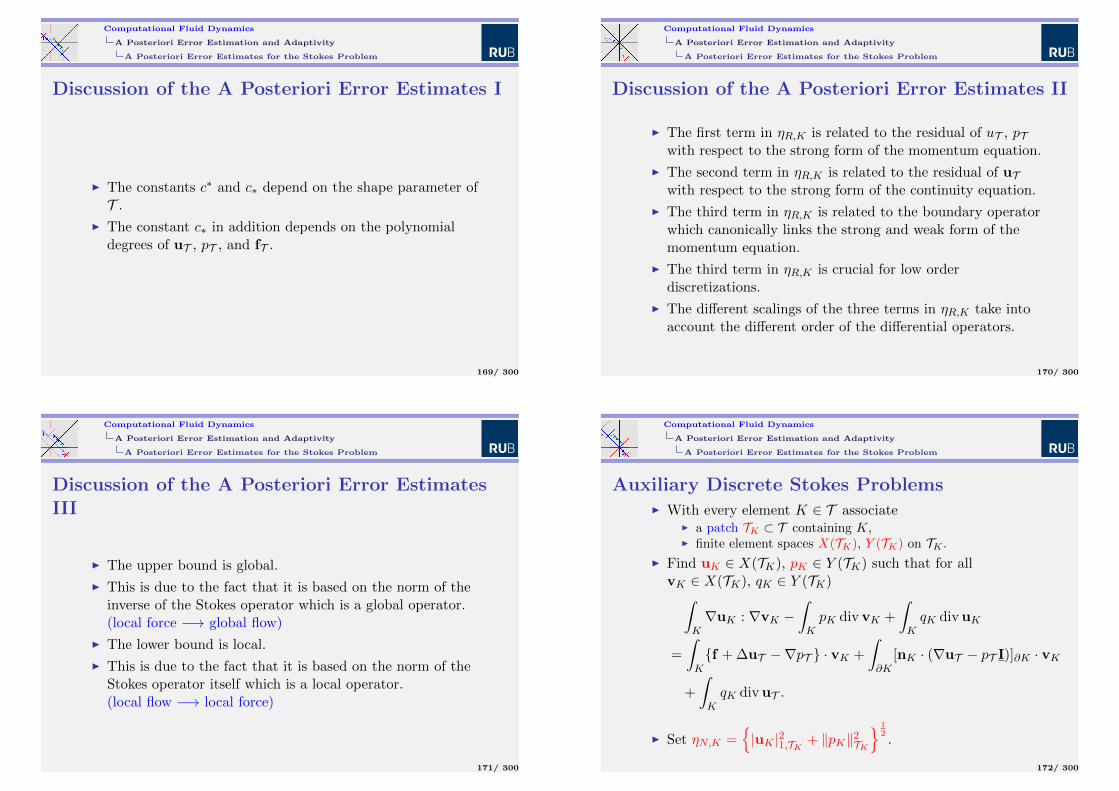
Computational Fluid Dynamics
A Posteriori Error Estimation and Adaptivity
A Posteriori Error Estimates for the Stokes Problem
Discussion of the A Posteriori Error Estimates I
I The constants c∗ and c∗ depend on the shape parameter ofT .
I The constant c∗ in addition depends on the polynomialdegrees of uT , pT , and fT .
169/ 300
Computational Fluid Dynamics
A Posteriori Error Estimation and Adaptivity
A Posteriori Error Estimates for the Stokes Problem
Discussion of the A Posteriori Error Estimates II
I The first term in ηR,K is related to the residual of uT , pTwith respect to the strong form of the momentum equation.
I The second term in ηR,K is related to the residual of uTwith respect to the strong form of the continuity equation.
I The third term in ηR,K is related to the boundary operatorwhich canonically links the strong and weak form of themomentum equation.
I The third term in ηR,K is crucial for low orderdiscretizations.
I The different scalings of the three terms in ηR,K take intoaccount the different order of the differential operators.
170/ 300
Computational Fluid Dynamics
A Posteriori Error Estimation and Adaptivity
A Posteriori Error Estimates for the Stokes Problem
Discussion of the A Posteriori Error EstimatesIII
I The upper bound is global.
I This is due to the fact that it is based on the norm of theinverse of the Stokes operator which is a global operator.(local force −→ global flow)
I The lower bound is local.
I This is due to the fact that it is based on the norm of theStokes operator itself which is a local operator.(local flow −→ local force)
171/ 300
Computational Fluid Dynamics
A Posteriori Error Estimation and Adaptivity
A Posteriori Error Estimates for the Stokes Problem
Auxiliary Discrete Stokes ProblemsI With every element K ∈ T associate
I a patch TK ⊂ T containing K,I finite element spaces X(TK), Y (TK) on TK .
I Find uK ∈ X(TK), pK ∈ Y (TK) such that for allvK ∈ X(TK), qK ∈ Y (TK)∫
K∇uK : ∇vK −
∫KpK divvK +
∫KqK divuK
=
∫Kf + ∆uT −∇pT · vK +
∫∂K
[nK · (∇uT − pT I)]∂K · vK
+
∫KqK divuT .
I Set ηN,K =|uK |21,TK + ‖pK‖2TK
12.
172/ 300
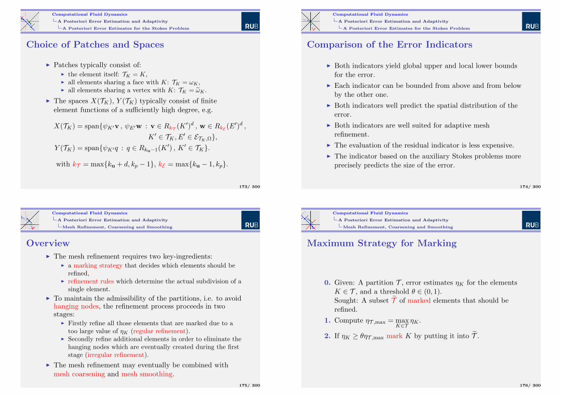
Computational Fluid Dynamics
A Posteriori Error Estimation and Adaptivity
A Posteriori Error Estimates for the Stokes Problem
Choice of Patches and Spaces
I Patches typically consist of:I the element itself: TK = K,I all elements sharing a face with K: TK = ωK ,I all elements sharing a vertex with K: TK = ωK .
I The spaces X(TK), Y (TK) typically consist of finiteelement functions of a sufficiently high degree, e.g.
X(TK) = spanψK′v , ψE′w : v ∈ RkT (K ′)d , w ∈ RkE (E′)d ,
K ′ ∈ TK , E′ ∈ ETK ,Ω,Y (TK) = spanψK′q : q ∈ Rku−1(K ′) , K ′ ∈ TK.
with kT = maxku + d, kp − 1, kE = maxku − 1, kp.
173/ 300
Computational Fluid Dynamics
A Posteriori Error Estimation and Adaptivity
A Posteriori Error Estimates for the Stokes Problem
Comparison of the Error Indicators
I Both indicators yield global upper and local lower boundsfor the error.
I Each indicator can be bounded from above and from belowby the other one.
I Both indicators well predict the spatial distribution of theerror.
I Both indicators are well suited for adaptive meshrefinement.
I The evaluation of the residual indicator is less expensive.
I The indicator based on the auxiliary Stokes problems moreprecisely predicts the size of the error.
174/ 300
Computational Fluid Dynamics
A Posteriori Error Estimation and Adaptivity
Mesh Refinement, Coarsening and Smoothing
OverviewI The mesh refinement requires two key-ingredients:
I a marking strategy that decides which elements should berefined,
I refinement rules which determine the actual subdivision of asingle element.
I To maintain the admissibility of the partitions, i.e. to avoidhanging nodes, the refinement process proceeds in twostages:
I Firstly refine all those elements that are marked due to atoo large value of ηK (regular refinement).
I Secondly refine additional elements in order to eliminate thehanging nodes which are eventually created during the firststage (irregular refinement).
I The mesh refinement may eventually be combined withmesh coarsening and mesh smoothing.
175/ 300
Computational Fluid Dynamics
A Posteriori Error Estimation and Adaptivity
Mesh Refinement, Coarsening and Smoothing
Maximum Strategy for Marking
0. Given: A partition T , error estimates ηK for the elementsK ∈ T , and a threshold θ ∈ (0, 1).Sought: A subset T of marked elements that should berefined.
1. Compute ηT ,max = maxK∈T
ηK .
2. If ηK ≥ θηT ,max mark K by putting it into T .
176/ 300
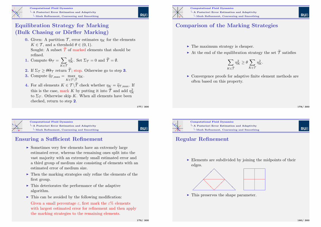
Computational Fluid Dynamics
A Posteriori Error Estimation and Adaptivity
Mesh Refinement, Coarsening and Smoothing
Equilibration Strategy for Marking(Bulk Chasing or Dorfler Marking)
0. Given: A partition T , error estimates ηK for the elementsK ∈ T , and a threshold θ ∈ (0, 1).Sought: A subset T of marked elements that should berefined.
1. Compute ΘT =∑K∈T
η2K . Set ΣT = 0 and T = ∅.
2. If ΣT ≥ θΘT return T ; stop. Otherwise go to step 3.
3. Compute ηT ,max = maxK∈T \T
ηK .
4. For all elements K ∈ T \T check whether ηK = ηT ,max. If
this is the case, mark K by putting it into T and add η2K
to ΣT . Otherwise skip K. When all elements have beenchecked, return to step 2.
177/ 300
Computational Fluid Dynamics
A Posteriori Error Estimation and Adaptivity
Mesh Refinement, Coarsening and Smoothing
Comparison of the Marking Strategies
I The maximum strategy is cheaper.
I At the end of the equilibration strategy the set T satisfies∑K∈T
η2K ≥ θ
∑K∈T
η2K .
I Convergence proofs for adaptive finite element methods areoften based on this property.
178/ 300
Computational Fluid Dynamics
A Posteriori Error Estimation and Adaptivity
Mesh Refinement, Coarsening and Smoothing
Ensuring a Sufficient Refinement
I Sometimes very few elements have an extremely largeestimated error, whereas the remaining ones split into thevast majority with an extremely small estimated error anda third group of medium size consisting of elements with anestimated error of medium size.
I Then the marking strategies only refine the elements of thefirst group.
I This deteriorates the performance of the adaptivealgorithm.
I This can be avoided by the following modification:
Given a small percentage ε, first mark the ε% elementswith largest estimated error for refinement and then applythe marking strategies to the remaining elements.
179/ 300
Computational Fluid Dynamics
A Posteriori Error Estimation and Adaptivity
Mesh Refinement, Coarsening and Smoothing
Regular Refinement
I Elements are subdivided by joining the midpoints of theiredges.
@
@@@@@
@@@
I This preserves the shape parameter.
180/ 300
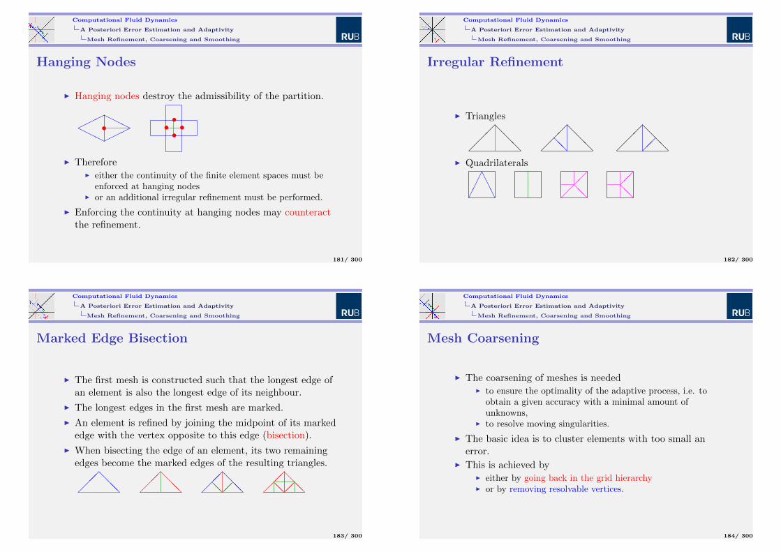
Computational Fluid Dynamics
A Posteriori Error Estimation and Adaptivity
Mesh Refinement, Coarsening and Smoothing
Hanging Nodes
I Hanging nodes destroy the admissibility of the partition.
H
HH
HHH• • •••
I ThereforeI either the continuity of the finite element spaces must be
enforced at hanging nodesI or an additional irregular refinement must be performed.
I Enforcing the continuity at hanging nodes may counteractthe refinement.
181/ 300
Computational Fluid Dynamics
A Posteriori Error Estimation and Adaptivity
Mesh Refinement, Coarsening and Smoothing
Irregular Refinement
I Triangles
@@@
@@@@@
@
@@
I Quadrilaterals
AAA
@@
@@
182/ 300
Computational Fluid Dynamics
A Posteriori Error Estimation and Adaptivity
Mesh Refinement, Coarsening and Smoothing
Marked Edge Bisection
I The first mesh is constructed such that the longest edge ofan element is also the longest edge of its neighbour.
I The longest edges in the first mesh are marked.
I An element is refined by joining the midpoint of its markededge with the vertex opposite to this edge (bisection).
I When bisecting the edge of an element, its two remainingedges become the marked edges of the resulting triangles.
@
@@ @
@@ @
@@@@ @
@@@@
183/ 300
Computational Fluid Dynamics
A Posteriori Error Estimation and Adaptivity
Mesh Refinement, Coarsening and Smoothing
Mesh Coarsening
I The coarsening of meshes is neededI to ensure the optimality of the adaptive process, i.e. to
obtain a given accuracy with a minimal amount ofunknowns,
I to resolve moving singularities.
I The basic idea is to cluster elements with too small anerror.
I This is achieved byI either by going back in the grid hierarchyI or by removing resolvable vertices.
184/ 300
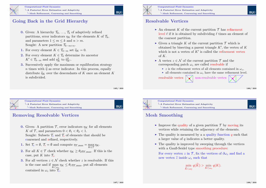
Computational Fluid Dynamics
A Posteriori Error Estimation and Adaptivity
Mesh Refinement, Coarsening and Smoothing
Going Back in the Grid Hierarchy
0. Given: A hierarchy T0, . . ., Tk of adaptively refinedpartitions, error indicators ηK for the elements K of Tk,and parameters 1 ≤ m ≤ k and n > m.Sought: A new partition Tk−m+n.
1. For every element K ∈ Tk−m set ηK = 0.
2. For every element K ∈ Tk determine its ancestorK ′ ∈ Tk−m and add η2
K to η2K′ .
3. Successively apply the maximum or equilibration strategyn times with η as error indicator. In this process, equallydistribute ηK over the descendants of K once an element Kis subdivided.
185/ 300
Computational Fluid Dynamics
A Posteriori Error Estimation and Adaptivity
Mesh Refinement, Coarsening and Smoothing
Resolvable Vertices
I An element K of the current partition T has refinementlevel ` if it is obtained by subdividing ` times an element ofthe coarsest partition.
I Given a triangle K of the current partition T which isobtained by bisecting a parent triangle K ′, the vertex of Kwhich is not a vertex of K ′ is called the refinement vertexof K.
I A vertex z ∈ N of the current partition T and thecorresponding patch ωz are called resolvable if
I z is the refinement vertex of all elements contained in ωz,I all elements contained in ωz have the same refinement level.
resolvable vertex @@@• non-resolvable vertex @
@@
•
186/ 300
Computational Fluid Dynamics
A Posteriori Error Estimation and Adaptivity
Mesh Refinement, Coarsening and Smoothing
Removing Resolvable Vertices
0. Given: A partition T , error indicators ηK for all elementsK of T , and parameters 0 < θ1 < θ2 < 1.Sought: Subsets Tc and Tr of elements that should becoarsened and refined, respectively.
1. Set Tc = ∅, Tr = ∅ and compute ηT ,max = maxK∈T
ηK .
2. For all K ∈ T check whether ηK ≥ θ2ηT ,max. If this is thecase, put K into Tr.
3. For all vertices z ∈ N check whether z is resolvable. If thisis the case and if max
K⊂ωzηK ≤ θ1ηT ,max, put all elements
contained in ωz into Tc.
187/ 300
Computational Fluid Dynamics
A Posteriori Error Estimation and Adaptivity
Mesh Refinement, Coarsening and Smoothing
Mesh Smoothing
I Improve the quality of a given partition T by moving itsvertices while retaining the adjacency of the elements.
I The quality is measured by a a quality function q such thata larger value of q indicates a better quality.
I The quality is improved by sweeping through the verticeswith a Gauß-Seidel type smoothing procedure:
For every vertex z in T , fix the vertices of ∂ωz and find anew vertex z inside ωz such that
minK⊂ωz
q(K) > minK⊂ωz
q(K).
188/ 300
Computational Fluid Dynamics
A Posteriori Error Estimation and Adaptivity
Mesh Refinement, Coarsening and Smoothing
Quality FunctionsI Based on geometric criteria:
q(K) =4√
3µ2(K)
µ1(E0)2 + µ1(E1)2 + µ1(E2)2
I Based on interpolation:
q(K) = ‖∇(uQ − uL)‖2Kwith linear and quadratic interpolants of u
I Based on an error indicator:
q(K) =
∫K
∣∣∣ 2∑i=0
ei∇ψEi∣∣∣2
with ei = h12Ei
[nEi · ∇uT ]Ei189/ 300
Computational Fluid Dynamics
Stationary Incompressible Navier-Stokes Equations
Stationary Incompressible Navier-StokesEquations
I Variational Formulation
I Discretization
I Solution of the Discrete Problems
I A Posteriori Error Estimates
190/ 300
Computational Fluid Dynamics
Stationary Incompressible Navier-Stokes Equations
Variational Formulation
Strong Form
I Stationary incompressible Navier-Stokes equations indimensionless form with no-slip boundary condition
−∆u +Re(u · ∇)u + grad p = f in Ω
divu = 0 in Ω
u = 0 on Γ
I For the variational formulation, we want to multiply themomentum equation with a test function v ∈ H1
0 (Ω)d andintegrate the result over Ω.
I This is possible if u ∈ H10 (Ω)d implies (u · ∇)u ∈ H−1(Ω)d.
191/ 300
Computational Fluid Dynamics
Stationary Incompressible Navier-Stokes Equations
Variational Formulation
Properties of the Non-Linear TermI Holder’s inequality yields for v ∈ H1
0 (Ω)d, u,w ∈ L4(Ω)d∫Ω
[(u · ∇)v
]·w ≤ ‖u‖L4(Ω)|v|1‖w‖L4(Ω).
I Since H10 (Ω) is continuously embedded in L4(Ω) for d ≤ 4
(compactly for d ≤ 3), this proves that[H1
0 (Ω)d]3 3 (u,v,w) 7→
∫Ω
[(u · ∇)v
]·w is a continuous
trilinear form.I Integration by parts yields for all u,v,w ∈ H1
0 (Ω)d withdivu = 0∫
Ω
[(u · ∇)v
]·w = −
∫Ω
[(u · ∇)w
]· v,
∫Ω
[(u ·∇)v
]·v = 0.
192/ 300
Computational Fluid Dynamics
Stationary Incompressible Navier-Stokes Equations
Variational Formulation
Variational Form
I Find u ∈ H10 (Ω)d, p ∈ L2
0(Ω) such that for all v ∈ H10 (Ω)d,
q ∈ L20(Ω)∫
Ω∇u : ∇v −
∫Ωp divv +
∫ΩRe[(u · ∇)u] · v =
∫Ωf · v∫
Ωq divu = 0
I Equivalent form:
Find u ∈ V such that for all v ∈ V∫Ω∇u : ∇v +
∫ΩRe[(u · ∇)u] · v =
∫Ωf · v
193/ 300
Computational Fluid Dynamics
Stationary Incompressible Navier-Stokes Equations
Variational Formulation
Fixed-Point Formulation
I Denote by T : H−1(Ω)d → V the Stokes operator whichassociates with g ∈ H−1(Ω)d the weak solution Tg = v ofthe Stokes problem with right-hand side g, i.e.∫
Ω∇v : ∇w =
∫Ωg ·w ∀w ∈ V.
I Then the variational formulation of the Navier-Stokesequations is equivalent to
u = T(f −Re(u · ∇)u
).
194/ 300
Computational Fluid Dynamics
Stationary Incompressible Navier-Stokes Equations
Variational Formulation
Properties of the Variational Problem
I Every solution satisfies the a priori bound|u|1 ≤ cF diam(Ω)‖f‖, where cF is the constant in theFriedrichs inequality.
I If Re 2d−1
2
[cF diam(Ω)
]3− d2 ‖f‖ < 1, there is at most one
solution.
I For every Reynolds’ number Re there exists at least onesolution.
I Every solution has the same regularity as the solution ofthe corresponding Stokes problem.
I Every solution belongs to a differentiable branch Re 7→ uReof solutions which has at most a countable number ofturning or bifurcation points.
195/ 300
Computational Fluid Dynamics
Stationary Incompressible Navier-Stokes Equations
Variational Formulation
A Priori Bound
Every solution u of the variational problem satisfies
|u|21 =
∫Ω∇u : ∇u
=
∫Ω∇u : ∇u +Re
∫Ω
[(u · ∇)u
]· u
=
∫Ωf · u
≤ ‖f‖‖u‖≤ ‖f‖cF diam(Ω)|u|1.
196/ 300
Computational Fluid Dynamics
Stationary Incompressible Navier-Stokes Equations
Variational Formulation
Uniqueness
I The difference v = u1 − u2 of any two solutions satisfies
|v|21 = −Re∫
Ω
[(u1 · ∇)u1
]· v +Re
∫Ω
[(u2 · ∇)u2
]· v
= −Re∫
Ω
[(u1 · ∇)v
]· v −Re
∫Ω
[(v · ∇)u2
]· v
= −Re∫
Ω
[(v · ∇)u2
]· v
≤ Re‖v‖2L4(Ω)|u2|1.
I Combined with the a priori bound, the estimate
‖v‖L4(Ω) ≤ 2d−1
4 ‖v‖1−d4 |v|
d41 and the Friedrichs inequality
this proves the uniqueness.
197/ 300
Computational Fluid Dynamics
Stationary Incompressible Navier-Stokes Equations
Variational Formulation
ExistenceI V is separable, i.e. there is as sequence of nested finite
dimensional subspaces Vm such that⋃m Vm is dense in V .
I Denote by Tm the Stokes operator corresponding to Vm.I The properties of the non-linear term and Schauder’s
fixed-point theorem imply that for every m there is aum ∈ Vm with um = Tm
(f −Re(um · ∇)um
).
I The arguments used to prove the a priori bound imply thatthe sequence um is bounded in H1.
I The compact embedding of H1 in L4 and the properties ofthe non-linear term imply that the um converge weakly toan u ∈ H1
0 (Ω)d which solves the variational problem withV replaced by anyone of the Vm.
I The density of⋃m Vm in V proves that u solves the
variational problem.
198/ 300
Computational Fluid Dynamics
Stationary Incompressible Navier-Stokes Equations
Variational Formulation
Regularity
The regularity is proved by a bootstrap-argument using thefixed-point equation u = T
(f −Re(u · ∇)u
)and the regularity
of the Stokes problem:
u ∈ H1 =⇒ u ∈ L6 =⇒ (u · ∇)u ∈ L53
=⇒ (u · ∇)u ∈ H−310 =⇒u ∈ H1+ 7
10
=⇒ u ∈ L∞ =⇒ (u · ∇)u ∈ L2
=⇒u ∈ H2
199/ 300
Computational Fluid Dynamics
Stationary Incompressible Navier-Stokes Equations
Variational Formulation
Branches of Solutions
I The fixed-point formulation implies that there are noisolated solutions and that every solution depends in adifferentiable way on Re.
I Differentiation of the fixed-point equation yields that v,the derivative w.r.t. Re of any solution u, satisfies
v = −ReT((u · ∇)v + (v · ∇)u
)− T
((u · ∇)u
).
I The compact embedding of H1 in L4 implies that theoperator w 7→ T
((u · ∇)w + (w · ∇)u
)is compact.
I The statement concerning limit and bifurcation pointstherefore follows from properties of the spectra of compactoperators, the Fredholm alternative and the a priori bound.
200/ 300
Computational Fluid Dynamics
Stationary Incompressible Navier-Stokes Equations
Discretization
Basic Idea
I Replace H10 (Ω)d, L2
0(Ω) by a pair X(T ), Y (T ) of finiteelement spaces which is uniformly stable for the Stokesproblem.
I Denote by V (T ) the corresponding approximation of V .
I Since V (T ) 6⊂ V the anti-symmetry of the non-linear termis lost.
I To recover the anti-symmetry replace the non-linear termby
N(u,v,w) =1
2
∫Ω
[(u · ∇)v
]·w − 1
2
∫Ω
[(u · ∇)w
]· v.
201/ 300
Computational Fluid Dynamics
Stationary Incompressible Navier-Stokes Equations
Discretization
Discrete Problem
I Find uT ∈ X(T ), pT ∈ Y (T ) such that for all vT ∈ X(T ),qT ∈ Y (T )∫
Ω∇uT : ∇vT −
∫ΩpT divvT +Re N(uT ,uT ,vT ) =
∫Ωf · vT∫
ΩqT divuT = 0
I Equivalent form:
Find uT ∈ V (T ) such that for all vT ∈ V (T )∫Ω∇uT : ∇vT +Re N(uT ,uT ,vT ) =
∫Ωf · vT
202/ 300
Computational Fluid Dynamics
Stationary Incompressible Navier-Stokes Equations
Discretization
Fixed-Point Formulation of the Discrete Problem
I Denote by TT : H−1(Ω)d → V (T ) the discrete Stokesoperator which associates with g ∈ H−1(Ω)d the weaksolution TT g = vT of the Stokes problem with right-handside g, i.e.∫
Ω∇vT : ∇wT =
∫Ωg ·wT ∀wT ∈ V (T ).
I Then the discrete problem is equivalent to
uT = TT(f −Re N(uT ,uT , ·)
).
203/ 300
Computational Fluid Dynamics
Stationary Incompressible Navier-Stokes Equations
Discretization
Properties of the Discrete Problem
I Every solution satisfies the a priori bound|uT |1 ≤ cF diam(Ω)‖f‖.
I If Re 2d−1
2
[cF diam(Ω)
]3− d2 ‖f‖ < 1, there is at most one
solution.
I For every Reynolds’ number Re there exists at least onesolution.
I Every solution belongs to a differentiable branchRe 7→ uT ,Re of solutions which has at most a finite numberof turning or bifurcation points.
204/ 300
Computational Fluid Dynamics
Stationary Incompressible Navier-Stokes Equations
Discretization
Error EstimatesI Assume that:
I Λ ⊂ (0,∞) is a compact, non empty interval.I Λ 3 Re 7→ uRe is a regular branch of solutions of the
Navier-Stokes equations.I uRe ∈ Hk+1(Ω)d, pRe ∈ Hk(Ω) for all Re ∈ Λ with k ≥ 1.I Sk,00 (T )d ⊂ X(T ) and Sk−1,−1(T ) ∩ L2
0(Ω) ⊂ Y (T ) orSmaxk−1,1,0(T ) ∩ L2
0(Ω) ⊂ Y (T ).
I Then there is a maximal mesh-size h0 = h0(Λ, f ,uRe) > 0such that for every partition T with hT ≤ h0 the discreteproblem has a solution uT ,Re ∈ X(T ), pT ,Re ∈ Y (T ) with
|uRe − uT ,Re|1 + ‖pRe − pT ,Re‖ ≤ chkT supRe∈Λ
|uRe|2k+1.
I ‖uRe − uT ,Re‖ ≤ chT |uRe − uT ,Re|1 if Ω is convex.
205/ 300
Computational Fluid Dynamics
Stationary Incompressible Navier-Stokes Equations
Discretization
Proof of the Error Estimates. The Basic Steps
I The continuous and discrete problem can be written asF (Re,uRe) = 0 and FT (Re,uT ,Re) = 0.
I FT evaluated at the H1-projection of uRe is small.
I The derivative of FT evaluated at the H1-projection of uReis close to the derivative of F evaluated at uRe.
I The derivative of FT evaluated at the H1-projection of uReis invertible.
I The derivative of FT is Lipschitz-continuous.
I The discrete problem has a solution in a neighbourhood ofthe H1-projection of uRe.
I Compare the obtained solution with the solution of theStokes problem with right-hand side f −Re (uRe · ∇)uRe.
206/ 300
Computational Fluid Dynamics
Stationary Incompressible Navier-Stokes Equations
Discretization
Proof of the Error Estimates. 1st StepAuxiliary quantities
I Define G, G ∈ C∞(H10 (Ω)d, H−1(Ω)d) by
〈G(v),w〉 =
∫Ω
[(v · ∇)v
]·w, 〈G(v),w〉 = N(v,v,w).
I Define F , FT ∈ C∞((0,∞)×H10 (Ω)d, H1
0 (Ω)d) by
F (Re,v) = v +ReTG(v)− T f ,
FT (Re,v) = v +ReTT G(v)− TT f .
I Note that F (Re,uRe) = 0 and FT (Re,uT ,Re) = 0.I Denote by uT ,Re the H1-projection of uRe on V (T ) and set
εT (Re) = |FT (Re, uT ,Re)|1.207/ 300
Computational Fluid Dynamics
Stationary Incompressible Navier-Stokes Equations
Discretization
Proof of the Error Estimates. 2nd Step
εT (Re) ≤ chkT supRe∈Λ
|uRe|2k+1
I εT (Re) = |FT (Re, uT ,Re)−F (Re,uRe)|1≤ |uRe − uT ,Re|1 +Re |TT (G(uT ,Re)− G(uRe))|1
+Re |(TT − T )G(uRe)|1 + |(T − TT )f |1I |uRe − uT ,Re|1 ≤ chkT |uRe|k+1
I |TT (G(uT ,Re)− G(uRe))|1 ≤ ‖G(uT ,Re)− G(uRe)‖−1
≤ c|uRe|1|uRe − uT ,Re|1I |(TT − T )G(uRe)|1 ≤ chkT ‖G(uRe)‖k−1 ≤ chkT |uRe|2k+1
I |(T − TT )f |1 ≤ chkT ‖f‖k−1 ≤ chT |uRe|k+1
208/ 300
Computational Fluid Dynamics
Stationary Incompressible Navier-Stokes Equations
Discretization
Proof of the Error Estimates. 3rd Step
‖|DvFT (Re, uT ,Re)−DvF (Re,uRe)‖| ≤ ch|uRe|2I DvFT (Re, uT ,Re)w −DvF (Re,uRe)w
= ReTT (DG(uT ,Re)w −DG(uRe)w)
+Re (TT − T )DG(uRe)w
I |TT (DG(uT ,Re)w −DG(uRe)w)|1≤ ‖DG(uT ,Re)w −DG(uRe)w‖−1
≤ chT |uRe|2|w|1I |(TT − T )DG(uRe)w|1 ≤ chT ‖DG(uRe)w‖
≤ chT |uRe|2|w|1
209/ 300
Computational Fluid Dynamics
Stationary Incompressible Navier-Stokes Equations
Discretization
Proof of the Error Estimates. 4th Step
‖|DvFT (Re, uT ,Re)−1‖| ≤ 2‖|DvF (Re,uRe)
−1‖| for sufficientlysmall hT
I ‖|A‖| ≤ 12 implies that (I −A) is invertible and satisfies
‖|(I −A)−1‖| ≤ 2
I DvFT (Re, uT ,Re)= DvF (Re,uRe)− [DvF (Re,uRe)−DvFT (Re, uT ,Re)]= DvF (Re,uRe)[I−
DvF (Re,uRe)−1(DvF (Re,uRe)−DvFT (Re, uT ,Re)]
210/ 300
Computational Fluid Dynamics
Stationary Incompressible Navier-Stokes Equations
Discretization
Proof of the Error Estimates. 5th Step
‖|DvFT (Re,v1)−DvFT (Re,v2)‖| ≤ cRe |v1 − v2|1I DvFT (Re,v1)w −DvFT (Re,v2)w
= ReTT (DG(v1)w −DG(v2)w)
I |TT (DG(v1)w −DG(v2)w)|1≤ ‖DG(v1)w −DG(v2)w‖−1
≤ c|v1 − v2|1|w|1
211/ 300
Computational Fluid Dynamics
Stationary Incompressible Navier-Stokes Equations
Discretization
Proof of the Error Estimates. 6th Step
The discrete problem has a solution uT ,Re with|uT ,Re − uT ,Re|1 ≤ 4‖|DvF (Re,uRe)
−1‖|εT (Re)
I Thanks to the fourth step we can define a mapping Φ by
Φ(v) = v −DvFT (Re, uT ,Re)−1FT (Re,v).
I Then uT ,Re is a solution of the discrete problem if and onlyif it is a fixed-point of Φ.
I The fourth and fifth step imply that Φ is a contraction onthe ball B in H1 with centre uT ,Re and radius4‖|DvF (Re,uRe)
−1‖|εT (Re).
212/ 300
Computational Fluid Dynamics
Stationary Incompressible Navier-Stokes Equations
Discretization
Proof of the Error Estimates. 7th Step
Proof of the error estimate
I The sixth step implies that|uRe − uT ,Re|1 ≤
(1 + 4‖|DvF (Re,uRe)
−1‖|)εT (Re).
I Set uT ,Re = TT (f − G(uRe)) and denote by pT ,Re thecorresponding pressure.
I The stability of the discretization implies|uT ,Re − uT ,Re|1 + ‖pT ,Re − pT ,Re‖≤ cRe ‖G(uRe)− G(uT ,Re)‖−1
≤ cRe(|uRe|1 + |uT ,Re|1
)|uRe − uT ,Re|1.
I The error estimates for the Stokes problem with right-handside f −Re (uRe · ∇)uRe yield|uT ,Re − uRe|1 + ‖pT ,Re − pRe‖ ≤ chkT |uRe|k+1.
213/ 300
Computational Fluid Dynamics
Stationary Incompressible Navier-Stokes Equations
Discretization
A Warning ExampleI Consider the two-point boundary value problem−u′′ +Reuu′ = 0 in (−1, 1) with boundary conditionsu(−1) = 1, u(1) = −1.
I The solution is u(x) = − tanh(αRex)tanh(αRe)
where the parameter
αRe is determined by the relation 2αRe tanh(αRe) = Re.I The solution exhibits a strong interior layer at x = 0.I Explicitly solving the difference equations shows that:
I central differences are unstable,
I one-sided differences with a constantorientation on the whole interval areunstable,
I one-sided differences with theirorientation depending on the sign ofu are stable.
214/ 300
Computational Fluid Dynamics
Stationary Incompressible Navier-Stokes Equations
Discretization
Conclusion
I We must stabilize the convective derivative.
I This can be achieved byI upwind schemes orI adding an artificial consistent viscosity in the direction of
the streamlines (streamline diffusion method or SDFEM inshort).
215/ 300
Computational Fluid Dynamics
Stationary Incompressible Navier-Stokes Equations
Discretization
An Upwind Scheme
I Approximate the integral involving the convectivederivative by a one-point quadrature rule∫
Ω[(uT ·∇)uT ]·vT ≈
∑K∈T|K|[(uT (xK)·∇)uT (xK)]·vT (xK).
I Replace the convective derivative by an up-wind difference
(uT (xK) · ∇)uT (xK) ≈ |uT (xK)||xK − yK |
(uT (xK)− uT (yK)).
I Replace uT (yK) by IT uT (yK), the linear interpolate of uTin the vertices of the face of K which contains yK .
yKb
a
xK
216/ 300
Computational Fluid Dynamics
Stationary Incompressible Navier-Stokes Equations
Discretization
Drawbacks of the Upwind Scheme
I It does not fit well into the framework of variationalmethods.
I The discrete problem is no longer differentiable.
217/ 300
Computational Fluid Dynamics
Stationary Incompressible Navier-Stokes Equations
Discretization
The Streamline Diffusion MethodFind uT ∈ X(T ) and pT ∈ Y (T ) such that for all vT , qT∫
Ω∇uT : ∇vT dx−
∫ΩpT divvT +
∫ΩRe[(uT · ∇)uT ] · vT
+∑K∈T
δKh2K
∫KRe[−f −∆uT +∇pT +Re(uT · ∇)uT ]·
· [(uT · ∇)vT ]
+∑K∈T
αKδK
∫K
divuT divvT =
∫Ωf · vT∫
ΩqT divuT +
∑E∈E
δEhE
∫E
[pT ]E [qT ]E
+∑K∈T
δKh2K
∫K
[−f −∆uT +∇pT +Re(uT · ∇)uT ] · ∇qT = 0
218/ 300
Computational Fluid Dynamics
Stationary Incompressible Navier-Stokes Equations
Discretization
Properties of the Streamline Diffusion Method
I It is able to simultaneously stabilize the effects of theconvection and of the divergence constraint.
I It gives rise to a differentiable discrete problem.
I Up to more technical arguments, its error analysis proceedsalong the lines indicated before.
I It yields the same error estimates as before without thestability condition for the finite element spaces.
I In a mesh-dependent norm, it in addition gives control on(uRe · ∇)(uRe − uT ,Re), the convective derivative of theerror.
219/ 300
Computational Fluid Dynamics
Stationary Incompressible Navier-Stokes Equations
Solution of the Discrete Problems
Potential Algorithms I
I Fixed-point iteration:I Requires the solution of Stokes problems.I Converges for sufficiently small Re.
I Newton iteration:I Requires the solution of linear Oseen problems with
potentially large convection.I Converges quadratically if the starting value is sufficiently
close to the solution.I May be combined with path-tracking.
I Path tracking:I Requires the solution of linear Oseen problems with
potentially large convection.I May yield reasonable starting values for the Newton
iteration.
220/ 300
Computational Fluid Dynamics
Stationary Incompressible Navier-Stokes Equations
Solution of the Discrete Problems
Potential Algorithms II
I Non-linear CG-algorithm of Polak-Ribiere:I Minimizes 1
2 |u− T (f −Re(u · ∇)u)|21.I Requires the solution of Stokes problems.
I Operator splitting:I Decouples the non-linearity and the incompressibility.I Requires the solution of Stokes problems and of non-linear
Poisson equations for the components of the velocity.
I Multigrid algorithms:I May either be applied to the linear problems in an inner
iteration or be used as an outer iteration with one of theabove methods as smoothing method.
221/ 300
Computational Fluid Dynamics
Stationary Incompressible Navier-Stokes Equations
Solution of the Discrete Problems
Fixed-Point Iteration
For i = 0, 1, . . . do:
I Solve the Stokes equations
−∆ui+1 +∇pi+1 = f −Re(ui · ∇)ui in Ω
divui+1 = 0 in Ω
ui+1 = 0 on Γ.
I If |ui+1 − ui|1 ≤ ε return ui+1, pi+1 as approximatesolution; stop.
222/ 300
Computational Fluid Dynamics
Stationary Incompressible Navier-Stokes Equations
Solution of the Discrete Problems
Newton Iteration
For i = 0, 1, . . . do:
I Solve the Oseen equations
−∆ui+1 +∇pi+1+Re(ui · ∇)ui+1
+Re(ui+1 · ∇)ui = f +Re(ui · ∇)ui in Ω
divui+1 = 0 in Ω
ui+1 = 0 on Γ.
I If |ui+1 − ui|1 ≤ ε return ui+1, pi+1 as approximatesolution; stop.
223/ 300
Computational Fluid Dynamics
Stationary Incompressible Navier-Stokes Equations
Solution of the Discrete Problems
Path Tracking
Given a Reynolds’ number λ, an increment ∆λ > 0 and anapproximate solution uλ for the Navier-Stokes equations withRe = λ.
I Solve the Oseen equations
−∆vλ +∇qλ + λ(uλ · ∇)vλ
+λ(vλ · ∇)uλ = f − λ(uλ · ∇)uλ in Ω
divvλ = 0 in Ω
vλ = 0 on Γ.
I Return uλ + ∆λvλ as approximate solution of theNavier-Stokes equations with Re = λ+ ∆λ.
224/ 300
Computational Fluid Dynamics
Stationary Incompressible Navier-Stokes Equations
Solution of the Discrete Problems
Operator SplittingFor i = 0, 1, . . . do:
I Solve the Stokes equations with no-slip boundary condition
2ωui+14 −∆ui+
14 +∇pi+
14 = 2ωui + f −Re(ui · ∇)ui
divui+14 = 0.
I Solve the non-linear Poisson equations with homogeneousboundary condition
ωui+34 −∆ui+
34 +Re(ui+
34 · ∇)ui+
34 = ωui+
14 + f −∇pi+
14 .
I Solve the Stokes equations with no-slip boundary condition
2ωui+1 −∆ui+1 +∇pi+1 = 2ωui+34 + f −Re(ui+
34 · ∇)ui+
34
divui+1 = 0.
I If |ui+1 − ui|1 ≤ ε return ui+1, pi+1; stop.225/ 300
Computational Fluid Dynamics
Stationary Incompressible Navier-Stokes Equations
A Posteriori Error Estimates
Basic Idea
I For regular branches of solutions, a quantitative form ofthe implicit function theorem implies that error andresidual are equivalent, i.e. the norm of the error can bebounded from above and from below by constant multiplesof the dual norm of the residual.
I The dual norm of the residual can be estimated as forlinear problems by
I either evaluating element-wise the residual with respect tothe strong form of the differential equation and suitableinter-element jumps
I or solving auxiliary local discrete linear problems.
I Limit and bifurcation points can be treated by suitablyaugmenting the residual.
226/ 300
Computational Fluid Dynamics
Stationary Incompressible Navier-Stokes Equations
A Posteriori Error Estimates
Equivalence of Error and ResidualI Assume that:
I (X, ‖·‖X), (Y, ‖·‖Y ) are Banach spaces.I F ∈ C1(X,Y ∗)I F (ϕ0) = 0I DF (ϕ0) is an isomorphism of X onto Y ∗.I ‖|DF (ϕ)−DF (ψ)‖| ≤ γ‖ϕ− ψ‖X for all ϕ, ψ in a ball with
centre ϕ0 and radius R0.
I Set R = minR0, γ
−1‖|DF (ϕ0)−1‖|−1, 2γ−1‖|DF (ϕ0)‖|
.
I Then, the following error estimates hold for all ϕ in a ballwith centre ϕ0 and radius R:
1
2‖|DF (ϕ0)‖|−1‖F (ϕ)‖Y ∗ ≤ ‖ϕ− ϕ0‖X
≤ 2‖|DF (ϕ0)−1‖|‖F (ϕ)‖Y ∗ .
227/ 300
Computational Fluid Dynamics
Stationary Incompressible Navier-Stokes Equations
A Posteriori Error Estimates
Proof of the EquivalenceI The upper bound for ‖ϕ− ϕ0‖X follows from
ϕ− ϕ0
= DF (ϕ0)−1DF (ϕ0)(ϕ− ϕ0) + F (ϕ)− F (ϕ) + F (ϕ0)
= DF (ϕ0)−1
F (ϕ)
+
∫ 1
0
[DF (ϕ0)−DF (ϕ0 + t(ϕ− ϕ0))
](ϕ− ϕ0)dt
.
I The lower bound for ‖ϕ− ϕ0‖X follows from
F (ϕ) = DF (ϕ0)(ϕ− ϕ0)
+
∫ 1
0
[DF (ϕ0 + t(ϕ− ϕ0))−DF (ϕ0)
](ϕ− ϕ0)dt.
228/ 300
Computational Fluid Dynamics
Stationary Incompressible Navier-Stokes Equations
A Posteriori Error Estimates
Residual A Posteriori Error Estimates
I Residual a posteriori error indicator:
ηR,K =h2K‖fT + ∆uT −Re (uT · ∇)uT −∇pT ‖2K
+ ‖divuT ‖2K
+1
2
∑E∈EK,Ω
hE‖[nE · (∇uT − pT I)
]E‖2E 1
2
I Upper bound:|u−uT |21 +‖p−pT ‖2
12 ≤ c∗
∑K∈T
(η2R,K+h2
K‖f−fT ‖2K) 1
2
I Lower bound:ηR,K ≤ c∗
|u− uT |21,ωK + ‖p− pT ‖2ωK + h2
K‖f − fT ‖2ωK 1
2
229/ 300
Computational Fluid Dynamics
Non-Stationary Incompressible Navier-Stokes Equations
Non-Stationary Incompressible Navier-StokesEquations
I Variational Formulation
I Finite Element Discretization
I Solution of the Discrete Problems
I A Posteriori Error Estimation and Adaptivity
230/ 300
Computational Fluid Dynamics
Non-Stationary Incompressible Navier-Stokes Equations
Variational Formulation
Strong Form
I Non-stationary incompressible Navier-Stokes equations indimensionless form with no-slip boundary condition
∂u
∂t−∆u +Re (u · ∇)u− grad p = f in Ω× (0, T )
divu = 0 in Ω× (0, T )
u = 0 on Γ× (0, T )
u(·, 0) = u0 in Ω
I We want to multiply the momentum equation with asuitable test function v and integrate over Ω× (0, T ).
I We need appropriate spaces of univariate functions withvalues in suitable Sobolev spaces.
231/ 300
Computational Fluid Dynamics
Non-Stationary Incompressible Navier-Stokes Equations
Variational Formulation
Function Spaces for Parabolic ProblemsI (U, ‖·‖U ), (W, ‖·‖W ) Banach spaces, U →W , 1 ≤ p ≤ ∞I Lp(a, b;U) all measurable functions u : (a, b)→ U such thatt 7→ ‖u(·, t)‖U is in Lp((a, b))
‖u‖Lp(a,b;U) =
∫ b
a‖u(·, t)‖pUdt
1p, if p <∞
ess. supt∈(a,b)
‖u(·, t)‖U , if p =∞
I W p(a, b;U,W ) =u ∈ Lp(a, b;U) : ∂tu ∈ Lp(a, b;W )
‖u‖W p(a,b;U,W ) =
∫ b
a‖u(·, t)‖pUdt+
∫ b
a‖∂u∂t
(·, t)‖pWdt 1p
ess. supt∈(a,b)
max‖u(·, t)‖U , ‖
∂u
∂t(·, t)‖W
232/ 300
Computational Fluid Dynamics
Non-Stationary Incompressible Navier-Stokes Equations
Variational Formulation
Properties of the Function Spaces
I Lp(a, b;U), W p(a, b;U,W ) are Banach spaces.
I ∂u∂t is defined in the distributional sense.
I Functions in W p(a, b;U,W ) have traces u(·, a), u(·, b) in Wif p > 1.
233/ 300
Computational Fluid Dynamics
Non-Stationary Incompressible Navier-Stokes Equations
Variational Formulation
Variational Form
Find u ∈ L2(0, T ;H10 (Ω)d), p ∈ L2(0, T ;L2
0(Ω)) such that for allv ∈W∞(0, T ;H1
0 (Ω)d, L2(Ω)d), q ∈ L∞(L20(Ω))∫ T
0
∫Ω
−u · ∂v
∂t+∇u : ∇v +Re [(u · ∇)u] · v − p divv
=
∫ T
0
∫Ωf · v+
∫Ωu0 · v(·, 0)∫ T
0
∫Ωq divu = 0
234/ 300
Computational Fluid Dynamics
Non-Stationary Incompressible Navier-Stokes Equations
Variational Formulation
Equivalent Variational Form
Find u ∈ L2(0, T ;V ) such that for all v ∈W∞(0, T ;V,L2(Ω)d)∫ T
0
∫Ω
−u · ∂v
∂t+∇u : ∇v +Re [(u · ∇)u] · v
=
∫ T
0
∫Ωf · v+
∫Ωu0 · v(·, 0)
235/ 300
Computational Fluid Dynamics
Non-Stationary Incompressible Navier-Stokes Equations
Variational Formulation
Properties of the Variational Problem
I For every Reynolds’ number Re, every right-hand sidef ∈ L2(0, T ;V ∗) and every initial value u0 ∈ L2(Ω)d withdivu0 = 0, there exists at least one solution. It satisfies∂u∂t ∈ L
1(0, T ;V ∗).
I If d = 2, there exists at most one solution. It satisfies∂u∂t ∈ L
2(0, T ;V ∗) and u ∈ C([0, T ], L2(Ω)2).
I If d = 3, every solution satisfies ∂u∂t ∈ L
43 (0, T ;V ∗) and
u ∈ L83 (0, T ;L4(Ω)3). There is at most one solution in
L2(0, T ;V ) ∩ L∞(0, T ;L2(Ω)3) ∩ L8(0, T ;L4(Ω)3). Everysuch solution satisfies u ∈ C([0, T ], L2(Ω)3).
236/ 300
Computational Fluid Dynamics
Non-Stationary Incompressible Navier-Stokes Equations
Variational Formulation
Existence. 1st Step
I V is separable, i.e. there is as sequence of nested finitedimensional subspaces Vm such that
⋃m Vm is dense in V .
I Denote by u0,m the L2-projection of u0 onto Vm.
I Recall that[H1
0 (Ω)d]3 3 (u,v,w) 7→
∫Ω
[(u · ∇)v
]·w is a
continuous anti-symmetric trilinear form.
237/ 300
Computational Fluid Dynamics
Non-Stationary Incompressible Navier-Stokes Equations
Variational Formulation
Existence. 2nd StepI The theorem of Picard-Lindelof implies that for every m
there is a maximal tm ∈ (0, T ] and a vm ∈ C1([0, tm], Vm)with vm(·, 0) = u0,m such that for all wm ∈ Vm∫
Ω
∂vm∂t·wm+∇vm : ∇wm +Re [(vm · ∇)vm] ·wm
=
∫Ωf ·wm.
I Inserting wm = vm yields
1
2
d
dt‖vm‖2 + |vm|21 =
∫Ω
∂vm∂t· vm + |vm|21
=
∫Ωf · vm ≤
1
2|vm|21 +
1
2|f |2−1.
238/ 300
Computational Fluid Dynamics
Non-Stationary Incompressible Navier-Stokes Equations
Variational Formulation
Existence. 3rd Step
I This implies lim supt→tm
‖vm(·, t)‖ <∞.
I Hence, tm = T and (vm) is contained in a bounded subsetof L∞(0, T ;L2(Ω)d) ∩ L2(0, T ;V ).
I A compactness theorem implies that there is au ∈ L∞(0, T ;L2(Ω)d) ∩ L2(0, T ;V ) such that vm → u
I weak in L2(0, T ;V ),I weak∗ in L∞(0, T ;L2(Ω)d),I strong in L2(0, T ;L2(Ω)d).
I The convergence allows to take the limit in the definingequation for the vm.
I Since⋃Vm is dense in V , this proves the existence.
239/ 300
Computational Fluid Dynamics
Non-Stationary Incompressible Navier-Stokes Equations
Variational Formulation
Uniqueness. 1st Step
I Define operators A, N on L∞(0, T ;L2(Ω)d) ∩ L2(0, T ;V )by
〈Au,v〉 =
∫Ω∇u : ∇v, 〈N(u),v〉 =
∫Ω
[(u · ∇)u
]· v.
I Then |N(u)|−1 ≤ ‖u‖2L4(Ω).
I Recall that ‖u‖L4(Ω) ≤ 2d−1
4 ‖u‖1−d4 |u|
d41 .
I Every solution of the variational problem satisfies
∂u
∂t+Au +N(u) = f in V ∗.
240/ 300
Computational Fluid Dynamics
Non-Stationary Incompressible Navier-Stokes Equations
Variational Formulation
Uniqueness. 2nd Step (d = 2)I Since |N(u)|−1 ≤
√2‖u‖|u|1, this proves that Au, N(u),
and ∂u∂t are all in L2(0, T ;V ∗).
I Embedding theorems yield the remaining regularity results.I The difference w = u1 − u2 of any two solutions satisfies
1
2
d
dt‖w(·, t)‖2 + |w|21 = 〈N(u1),w〉 − 〈N(u2),w〉
=
∫Ω
[(w · ∇)u1
]·w ≤
√2|w|1‖w‖|u1|1
⇒ d
dt‖w(·, t)‖2 ≤ |u1(·, t)|21‖w(·, t)‖2
⇒ d
dt
‖w(·, t)‖2 exp
[−∫ t
0|u1(·, s)|21ds
]≤ 0.
I Since u1 ∈ L2(0, T ;V ) and w(·, 0) = 0, this proves w = 0.
241/ 300
Computational Fluid Dynamics
Non-Stationary Incompressible Navier-Stokes Equations
Variational Formulation
Uniqueness. 3rd Step (d = 3)
I Since now |N(u)|−1 ≤ ‖u‖2L4(Ω) ≤ 2‖u‖12 |u|
321 , we have
Au ∈ L2(0, T ;V ∗) and N(u), ∂u∂t in L
43 (0, T ;V ∗).
I Embedding theorems yield the remaining regularity results.I The difference w = u1 − u2 of any two solutions now
satisfies
1
2
d
dt‖w(·, t)‖2 + |w|21 =
∫Ω
[(w · ∇)u1
]·w
= −∫
Ω
[(w · ∇)w
]· u1 ≤ 2|w|
741 ‖w‖
14 ‖u1‖L4(Ω)
⇒ d
dt‖w(·, t)‖2 ≤ 1
2
(7
4
)7‖u1(·, t)‖8L4(Ω)‖w(·, t)‖2
I Since u1 ∈ L8(0, T ;L4(Ω)3) and w(·, 0) = 0, this provesw = 0.
242/ 300
Computational Fluid Dynamics
Non-Stationary Incompressible Navier-Stokes Equations
Variational Formulation
Regularity of Solutions
I Assume thatI d = 2,I Γ ∈ C2,I f ∈ L∞(0, T ;L2(Ω)2), ∂f
∂t ∈ L2(0, T ;V ∗), div f = 0,
I u0 ∈ H2(Ω)2 ∩ V ,
I then the solution is in L∞(0, T ;H2(Ω)2).
I Assume thatI d = 3,I Γ ∈ C∞,I f ∈ L∞(0, T ;L2(Ω)3), ∂f
∂t ∈ L1(0, T ;L2(Ω)3), div f = 0,
I u0 ∈ H2(Ω)3 ∩ V ,I ‖f(·, 0)‖, ‖f‖L∞(0,T ;V ∗) and ‖u0‖2 are sufficiently small,
I then the there is a unique solution withu ∈ L∞(0, T ;H2(Ω)3), ∂u∂t ∈ L
2(0, T ;V )∩L∞(0, T ;L2(Ω)3).
243/ 300
Computational Fluid Dynamics
Non-Stationary Incompressible Navier-Stokes Equations
Variational Formulation
Further Regularity of SolutionsI The above regularity results do not suffice to prove second
order error estimates w.r.t. time.I In order to obtain such estimates, the quantities
|∂u∂t
(·, t)|1,∫ T
t‖∂u∂t
(·, s)‖22ds,∫ T
t‖∂
2u
∂t2(·, s)‖2ds
must remain bounded for t→ 0.I If any of these quantities remains bounded, the following
overdetermined Neumann problem admits a uniquesolution:
∆ϕ = div(f(·, 0)− (u0∇)u0
)in Ω
∇ϕ = ∆u0 + f(·, 0)− (u0∇)u0 on Γ.
I This is a non-local compatibility condition.
244/ 300
Computational Fluid Dynamics
Non-Stationary Incompressible Navier-Stokes Equations
Finite Element Discretization
Discretization of Parabolic Problems
I There are three main approaches for the discretization ofparabolic problems:
I Method of lines,I Rothe’s method,I Space-Time Finite Elements.
I For classical non-adaptive discretizations all approachesoften yield the same discrete solution.
I The method of lines is very inflexible w.r.t. to adaptivity.
I The error analysis of Rothe’s method is very intricate sinceit requires regularity results w.r.t. time which often are notavailable.
I Space-time finite elements are well amenable to a posteriorierror estimation and space and time adaptivity.
245/ 300
Computational Fluid Dynamics
Non-Stationary Incompressible Navier-Stokes Equations
Finite Element Discretization
Basic Idea of the Method of Lines
I Choose a fixed spatial mesh and associated finite elementspaces.
I Apply a standard ODE-solver (e.g. implicit Euler,Crank-Nicolson, Runge-Kutta, . . .) to the resulting systemof ordinary differential equations.
246/ 300
Computational Fluid Dynamics
Non-Stationary Incompressible Navier-Stokes Equations
Finite Element Discretization
Discretization of the Navier-Stokes Equationswith the Method of Lines
I Choose a spatial mesh T and associated finite elementspaces X(T ), Y (T ) which are uniformly stable for theStokes problem.
I Denote by AT , BT and NT (uT ) the associated stiffnessmatrices.
I Then the spatial discretization yields the following systemof differential-algebraic equations:
duTdt
= fT − νAT uT −BT pT −NT (uT )
BTT uT = 0.
247/ 300
Computational Fluid Dynamics
Non-Stationary Incompressible Navier-Stokes Equations
Finite Element Discretization
Temporal Discretization with the θ-Scheme
I Applying the θ-scheme to the above system requires tocompute an appropriate interpolate u0
T = RT u0 of theinitial value and, for n = 1, 2, . . ., to solve the discretestationary Navier-Stokes problems
unT − un−1T
τn= −BT pnT + θ fnT − νAT unT −NT (unT )
+ (1− θ)fn−1T − νAT un−1
T −NT (un−1T )
BTT u
nT = 0
I The choice θ = 12 corresponds to the Crank-Nicolson
scheme, θ = 1 to the implicit Euler scheme.
248/ 300
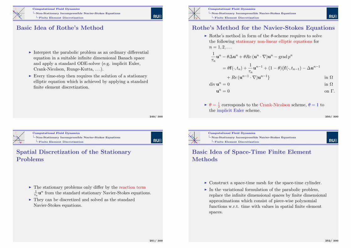
Computational Fluid Dynamics
Non-Stationary Incompressible Navier-Stokes Equations
Finite Element Discretization
Basic Idea of Rothe’s Method
I Interpret the parabolic problem as an ordinary differentialequation in a suitable infinite dimensional Banach spaceand apply a standard ODE-solver (e.g. implicit Euler,Crank-Nicolson, Runge-Kutta, . . .).
I Every time-step then requires the solution of a stationaryelliptic equation which is achieved by applying a standardfinite element discretization.
249/ 300
Computational Fluid Dynamics
Non-Stationary Incompressible Navier-Stokes Equations
Finite Element Discretization
Rothe’s Method for the Navier-Stokes EquationsI Rothe’s method in form of the θ-scheme requires to solve
the following stationary non-linear elliptic equations forn = 1, 2, . . .
1
τnun − θ∆un + θRe (un · ∇)un − grad pn
= θf(·, tn) +1
τnun−1 + (1− θ)f(·, tn−1)−∆un−1
+Re (un−1 · ∇)un−1 in Ω
divun = 0 in Ω
un = 0 on Γ.
I θ = 12 corresponds to the Crank-Nicolson scheme, θ = 1 to
the implicit Euler scheme.250/ 300
Computational Fluid Dynamics
Non-Stationary Incompressible Navier-Stokes Equations
Finite Element Discretization
Spatial Discretization of the StationaryProblems
I The stationary problems only differ by the reaction term1τnun from the standard stationary Navier-Stokes equations.
I They can be discretized and solved as the standardNavier-Stokes equations.
251/ 300
Computational Fluid Dynamics
Non-Stationary Incompressible Navier-Stokes Equations
Finite Element Discretization
Basic Idea of Space-Time Finite ElementMethods
I Construct a space-time mesh for the space-time cylinder.
I In the variational formulation of the parabolic problem,replace the infinite dimensional spaces by finite dimensionalapproximations which consist of piece-wise polynomialfunctions w.r.t. time with values in spatial finite elementspaces.
252/ 300
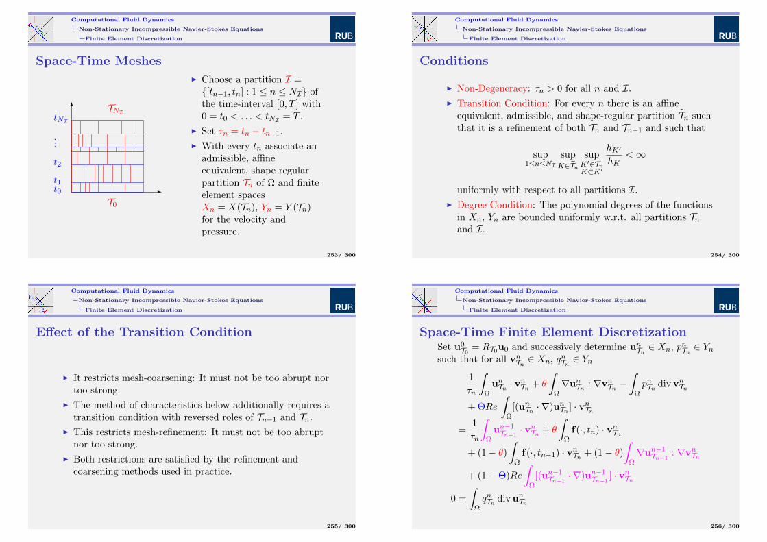
Computational Fluid Dynamics
Non-Stationary Incompressible Navier-Stokes Equations
Finite Element Discretization
Space-Time Meshes
-
6
t0t1
t2
...
tNI
T0
TNI
I Choose a partition I =[tn−1, tn] : 1 ≤ n ≤ NI ofthe time-interval [0, T ] with0 = t0 < . . . < tNI = T .
I Set τn = tn − tn−1.
I With every tn associate anadmissible, affineequivalent, shape regularpartition Tn of Ω and finiteelement spacesXn = X(Tn), Yn = Y (Tn)for the velocity andpressure.
253/ 300
Computational Fluid Dynamics
Non-Stationary Incompressible Navier-Stokes Equations
Finite Element Discretization
Conditions
I Non-Degeneracy: τn > 0 for all n and I.
I Transition Condition: For every n there is an affineequivalent, admissible, and shape-regular partition Tn suchthat it is a refinement of both Tn and Tn−1 and such that
sup1≤n≤NI
supK∈Tn
supK′∈TnK⊂K′
hK′
hK<∞
uniformly with respect to all partitions I.
I Degree Condition: The polynomial degrees of the functionsin Xn, Yn are bounded uniformly w.r.t. all partitions Tnand I.
254/ 300
Computational Fluid Dynamics
Non-Stationary Incompressible Navier-Stokes Equations
Finite Element Discretization
Effect of the Transition Condition
I It restricts mesh-coarsening: It must not be too abrupt nortoo strong.
I The method of characteristics below additionally requires atransition condition with reversed roles of Tn−1 and Tn.
I This restricts mesh-refinement: It must not be too abruptnor too strong.
I Both restrictions are satisfied by the refinement andcoarsening methods used in practice.
255/ 300
Computational Fluid Dynamics
Non-Stationary Incompressible Navier-Stokes Equations
Finite Element Discretization
Space-Time Finite Element DiscretizationSet u0
T0 = RT0u0 and successively determine unTn ∈ Xn, pnTn ∈ Ynsuch that for all vnTn ∈ Xn, qnTn ∈ Yn
1
τn
∫ΩunTn · v
nTn + θ
∫Ω∇unTn : ∇vnTn −
∫ΩpnTn divvnTn
+ ΘRe
∫Ω
[(unTn · ∇)unTn ] · vnTn
=1
τn
∫Ωun−1Tn−1
· vnTn + θ
∫Ωf(·, tn) · vnTn
+ (1− θ)∫
Ωf(·, tn−1) · vnTn + (1− θ)
∫Ω∇un−1Tn−1
: ∇vnTn
+ (1−Θ)Re
∫Ω
[(un−1Tn−1
· ∇)un−1Tn−1
] · vnTn
0 =
∫ΩqnTn divunTn
256/ 300
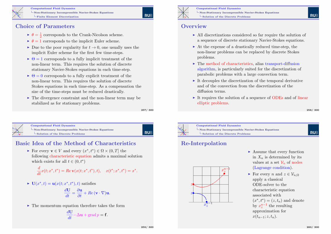
Computational Fluid Dynamics
Non-Stationary Incompressible Navier-Stokes Equations
Finite Element Discretization
Choice of Parameters
I θ = 12 corresponds to the Crank-Nicolson scheme.
I θ = 1 corresponds to the implicit Euler scheme.
I Due to the poor regularity for t→ 0, one usually uses theimplicit Euler scheme for the first few time-steps.
I Θ = 1 corresponds to a fully implicit treatment of thenon-linear term. This requires the solution of discretestationary Navier-Stokes equations in each time-step.
I Θ = 0 corresponds to a fully explicit treatment of thenon-linear term. This requires the solution of discreteStokes equations in each time-step. As a compensation thesize of the time-steps must be reduced drastically.
I The divergence constraint and the non-linear term may bestabilized as for stationary problems.
257/ 300
Computational Fluid Dynamics
Non-Stationary Incompressible Navier-Stokes Equations
Solution of the Discrete Problems
Overview
I All discretizations considered so far require the solution ofa sequence of discrete stationary Navier-Stokes equations.
I At the expense of a drastically reduced time-step, thenon-linear problems can be replaced by discrete Stokesproblems.
I The method of characteristics, alias transport-diffusionalgorithm, is particularly suited for the discretization ofparabolic problems with a large convection term.
I It decouples the discretization of the temporal derivativeand of the convection from the discretization of thediffusion terms.
I It requires the solution of a sequence of ODEs and of linearelliptic problems.
258/ 300
Computational Fluid Dynamics
Non-Stationary Incompressible Navier-Stokes Equations
Solution of the Discrete Problems
Basic Idea of the Method of CharacteristicsI For every v ∈ V and every (x∗, t∗) ∈ Ω× (0, T ] the
following characteristic equation admits a maximal solutionwhich exists for all t ∈ (0, t∗)
d
dtx(t;x∗, t∗) = Rev(x(t;x∗, t∗), t), x(t∗;x∗, t∗) = x∗.
I U(x∗, t) = u(x(t;x∗, t∗), t) satisfies
dU
dt=∂u
∂t+Re (v · ∇)u.
I The momentum equation therefore takes the form
dU
dt−∆u + grad p = f .
259/ 300
Computational Fluid Dynamics
Non-Stationary Incompressible Navier-Stokes Equations
Solution of the Discrete Problems
Re-Interpolation
z•
•xn−1z
z•
•xn−1z
I Assume that every functionin Xn is determined by itsvalues at a set Vn of nodes(Lagrange condition).
I For every n and z ∈ Vn,Ωapply a classicalODE-solver to thecharacteristic equationassociated with(x∗, t∗) = (z, tn) and denoteby xn−1
z the resultingapproximation forx(tn−1; z, tn).
260/ 300
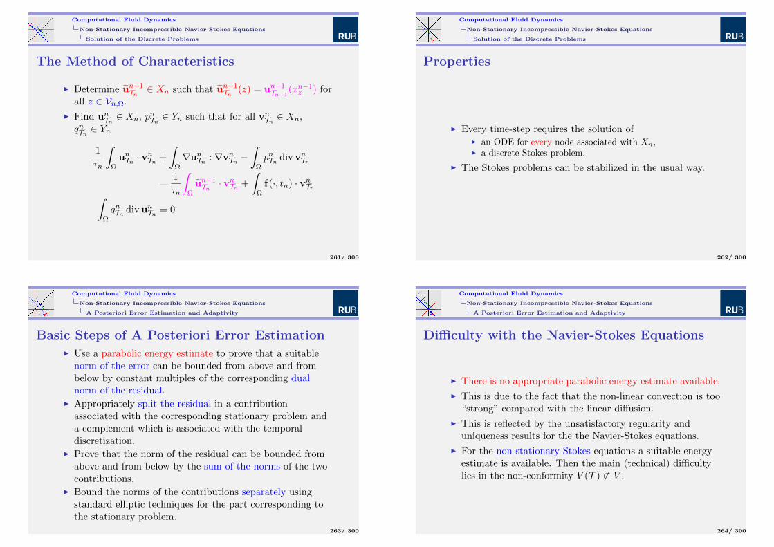
Computational Fluid Dynamics
Non-Stationary Incompressible Navier-Stokes Equations
Solution of the Discrete Problems
The Method of Characteristics
I Determine un−1Tn ∈ Xn such that un−1
Tn (z) = un−1Tn−1
(xn−1z ) for
all z ∈ Vn,Ω.
I Find unTn ∈ Xn, pnTn ∈ Yn such that for all vnTn ∈ Xn,qnTn ∈ Yn
1
τn
∫ΩunTn · v
nTn +
∫Ω∇unTn : ∇vnTn −
∫ΩpnTn divvnTn
=1
τn
∫Ωun−1Tn · v
nTn +
∫Ωf(·, tn) · vnTn∫
ΩqnTn divunTn = 0
261/ 300
Computational Fluid Dynamics
Non-Stationary Incompressible Navier-Stokes Equations
Solution of the Discrete Problems
Properties
I Every time-step requires the solution ofI an ODE for every node associated with Xn,I a discrete Stokes problem.
I The Stokes problems can be stabilized in the usual way.
262/ 300
Computational Fluid Dynamics
Non-Stationary Incompressible Navier-Stokes Equations
A Posteriori Error Estimation and Adaptivity
Basic Steps of A Posteriori Error EstimationI Use a parabolic energy estimate to prove that a suitable
norm of the error can be bounded from above and frombelow by constant multiples of the corresponding dualnorm of the residual.
I Appropriately split the residual in a contributionassociated with the corresponding stationary problem anda complement which is associated with the temporaldiscretization.
I Prove that the norm of the residual can be bounded fromabove and from below by the sum of the norms of the twocontributions.
I Bound the norms of the contributions separately usingstandard elliptic techniques for the part corresponding tothe stationary problem.
263/ 300
Computational Fluid Dynamics
Non-Stationary Incompressible Navier-Stokes Equations
A Posteriori Error Estimation and Adaptivity
Difficulty with the Navier-Stokes Equations
I There is no appropriate parabolic energy estimate available.
I This is due to the fact that the non-linear convection is too“strong” compared with the linear diffusion.
I This is reflected by the unsatisfactory regularity anduniqueness results for the the Navier-Stokes equations.
I For the non-stationary Stokes equations a suitable energyestimate is available. Then the main (technical) difficultylies in the non-conformity V (T ) 6⊂ V .
264/ 300
Computational Fluid Dynamics
Non-Stationary Incompressible Navier-Stokes Equations
A Posteriori Error Estimation and Adaptivity
A Residual Error Indicator for theNon-Stationary Stokes Equations
I Spatial error indicator
ηnh = ∑K∈Tn
h2K‖f(·, tn)− 1
τn(unTn − un−1
Tn−1) + ∆unTn −∇p
nTn‖
2K
+∑
E∈En,Ω
hE‖[nE · (∇unTn − pnTnI)]E‖
2E
+∑K∈Tn
‖divunTn‖2K
12
I Temporal error indicator
ηnτ =‖∇(unTn − un−1
Tn−1)‖2 + ‖div(unTn − un−1
Tn−1)‖2 1
2
265/ 300
Computational Fluid Dynamics
Non-Stationary Incompressible Navier-Stokes Equations
A Posteriori Error Estimation and Adaptivity
A Posteriori Error Estimates for theNon-Stationary Stokes Equations
I Denote by uI the continuous, temporally piece-wise affinefunction which coincides with unTn at time tn and by pI thetemporally piece-wise constant function which coincideswith pnTn on (tn−1, tn].
I Then‖∂t(u− uI) +∇(p− pI)‖2L2(0,T ;H−1(Ω)d)
+ ‖u− uI‖2L∞(0,T ;L2(Ω)d) + ‖u− uI‖2L2(0,T ;H10 (Ω)d)
12
≈‖u0T0 − u0‖2 +
NI∑n=1
τn[(ηnh)2
+(ηnτ)2] 1
2
266/ 300
Computational Fluid Dynamics
Non-Stationary Incompressible Navier-Stokes Equations
A Posteriori Error Estimation and Adaptivity
Modifications for the Navier-Stokes Equations
I Add the non-linear term Re (unTn · ∇)unTn to the elementresiduals in ηnh .
I For every n determine unTn ∈ S1,00 (Tn)d such that for all
vnTn ∈ S1,00 (Tn)d∫Ω∇unTn : ∇vnTn = Re
∫Ω
[(unTn · ∇)unTn
]· vnTn .
I Augment(ηnτ)2
by
|unTn |21 +
∑K∈Tn
h2K‖∆unTn +Re (unTn · ∇)(unTn − un−1
Tn−1)‖2K .
267/ 300
Computational Fluid Dynamics
Non-Stationary Incompressible Navier-Stokes Equations
A Posteriori Error Estimation and Adaptivity
An Algorithm for Space-Time Adaptivity
0. Given a tolerance ε, an initial mesh T0 and an initialtime-step τ1.
1. Refine T0 until ‖RT0u0 − u0‖ ≤ ε√2, set n = 1, t1 = τ1.
2. Solve the discrete problem on time-level n and determinethe error indicators ηnh and ηnτ .
3. If ηnτ >ε
2√T
, replace tn by 12(tn−1 + tn) and return to 2.
4. Apply a standard mesh-refinement and coarseningalgorithm to the discrete problem on time-level n with thecurrent time-step τn until ηnh ≤
ε2√T
. If ηnτ <ε
4√T
, replace
τn by 2τn.
5. If tn = T , stop. Otherwise set tn+1 = minT, tn + τn,increment n by 1 and return to 2.
268/ 300
Computational Fluid Dynamics
Compressible and Inviscid Problems
Compressible and Inviscid Problems
I Systems in Divergence Form
I Discretization
269/ 300
Computational Fluid Dynamics
Compressible and Inviscid Problems
Systems in Divergence Form
The SettingI Domain: Ω ⊂ RdI Source: g : Rm × Ω× (0,∞)→ RmI Mass: M : Rm → RmI Flux: F : Rm → Rm×dI Initial value: U0 : Ω→ RmI Problem: Find U : Ω× (0,∞)→ Rm such that under
appropriate boundary conditions
∂M(U)
∂t+ divF(U) = g(U, x, t) in Ω× (0,∞)
U(·, 0) = U0 in Ω
I divF(U) =( d∑j=1
∂F(U)i,j∂xj
)1≤i≤m
270/ 300
Computational Fluid Dynamics
Compressible and Inviscid Problems
Systems in Divergence Form
Advective and Viscous Fluxes
I The flux F splits into two contributions F = Fadv + Fvisc.
I Fadv is called advective flux and contains no derivatives.
I Fvisc is called viscous flux and contains spatial derivatives.
I The advective flux stems from the transport theorem andmodels transport or convection phenomena.
I The viscous flux models viscosity or diffusion phenomena.
271/ 300
Computational Fluid Dynamics
Compressible and Inviscid Problems
Systems in Divergence Form
Euler Equations
m = d+ 2 U =
ρve
M(U) =
ρρve
g =
0ρff · v
Fadv(U) =
ρvρv ⊗ v + pIev + pv
272/ 300
Computational Fluid Dynamics
Compressible and Inviscid Problems
Systems in Divergence Form
Compressible Navier-Stokes Equations inConservative Form
m = d+ 2 U =
ρve
M(U) =
ρρve
g =
0ρff · v
Fadv(U) =
ρvρv ⊗ v + pIev + pv
Fvisc(U) =
0T + pI
(T + pI) · v + σ
273/ 300
Computational Fluid Dynamics
Compressible and Inviscid Problems
Systems in Divergence Form
An Existence and Uniqueness ResultI Assume that
I the boundary Γ is sufficiently smooth,I the exterior forces are sufficiently smooth,I the initial data ρ0, u0, p0 and the exterior forces satisfy
appropriate compatibility conditions of the form
u0 · n = 0 on Γ
∂u0
∂t· n = 0 on Γ(∂f
∂t− (
∂u0
∂t· ∇)u0 − (u0 · ∇)
∂u0
∂t
+∇(ρ−1
0 p0 div(ρ0u0)))· n = 0 on Γ.
I Then the compressible Navier-Stokes and Euler equationsadmit a unique solution on a small time interval.
274/ 300
Computational Fluid Dynamics
Compressible and Inviscid Problems
Systems in Divergence Form
Remarks
I The previous result is proved by a fixed-point argument.
I Long-time existence results require conditions of the form“initial data and exterior forces sufficiently small”.
I Existence results under weaker assumptions can be provedusing the concept of compensated compactness.
I Uniqueness results typically require some sort of entropycondition.
275/ 300
Computational Fluid Dynamics
Compressible and Inviscid Problems
Discretization
Most Popular Methods
I Finite Volume Methods
Discretize the integral form of the system using piece-wiseconstant approximations on a mesh consisting ofpolyhedral cells combined with suitable numericalapproximations for the fluxes across the cells’ boundaries.
I Discontinuous Galerkin Methods
Discretize a suitable weak formulation of the system usingdiscontinuous piece-wise polynomial approximationscombined with appropriate stabilization terms.
276/ 300
Computational Fluid Dynamics
Compressible and Inviscid Problems
Discretization
Finite Volume Discretization. 1st Step
I Choose a time-step τ > 0.
I Choose a partition T of the domain Ω consisting ofarbitrary non-overlapping polyhedra.
I Fix n ∈ N∗ and K ∈ T .
I Integrate the system over K × [(n− 1)τ, nτ ]:∫ nτ
(n−1)τ
∫K
∂M(U)
∂t+
∫ nτ
(n−1)τ
∫K
divF(U)
=
∫ nτ
(n−1)τ
∫Kg(U, x, t)
277/ 300
Computational Fluid Dynamics
Compressible and Inviscid Problems
Discretization
Finite Volume Discretization. 2nd Step
Use integration by parts for the terms on the left-hand side:∫ nτ
(n−1)τ
∫K
∂M(U)
∂t=
∫KM(U(x, nτ))
−∫KM(U(x, (n− 1)τ))∫ nτ
(n−1)τ
∫K
divF(U) =
∫ nτ
(n−1)τ
∫∂K
F(U) · nK
278/ 300
Computational Fluid Dynamics
Compressible and Inviscid Problems
Discretization
Finite Volume Discretization. 3rd Step
I Assume that U is piecewise constant with respect to spaceand time.
I Denote by UnK and Un−1
K its constant values on K at timesnτ and (n− 1)τ respectively:∫
KM(U(x, nτ)) ≈ |K|M(Un
K)∫KM(U(x, (n− 1)τ)) ≈ |K|M(Un−1
K )∫ nτ
(n−1)τ
∫∂K
F(U) · nK ≈ τ∫∂K
F(Un−1K ) · nK∫ nτ
(n−1)τ
∫Kg(U, x, t) ≈ τ |K|g(Un−1
K , xK , (n− 1)τ)
279/ 300
Computational Fluid Dynamics
Compressible and Inviscid Problems
Discretization
Finite Volume Discretization. 4th Step
Approximate the boundary integral for the flux by a numericalflux:
τ
∫∂K
F(Un−1K ) · nK ≈ τ
∑K′∈T
∂K∩∂K′∈E
|∂K ∩ ∂K ′|FT (Un−1K ,Un−1
K′ )
280/ 300
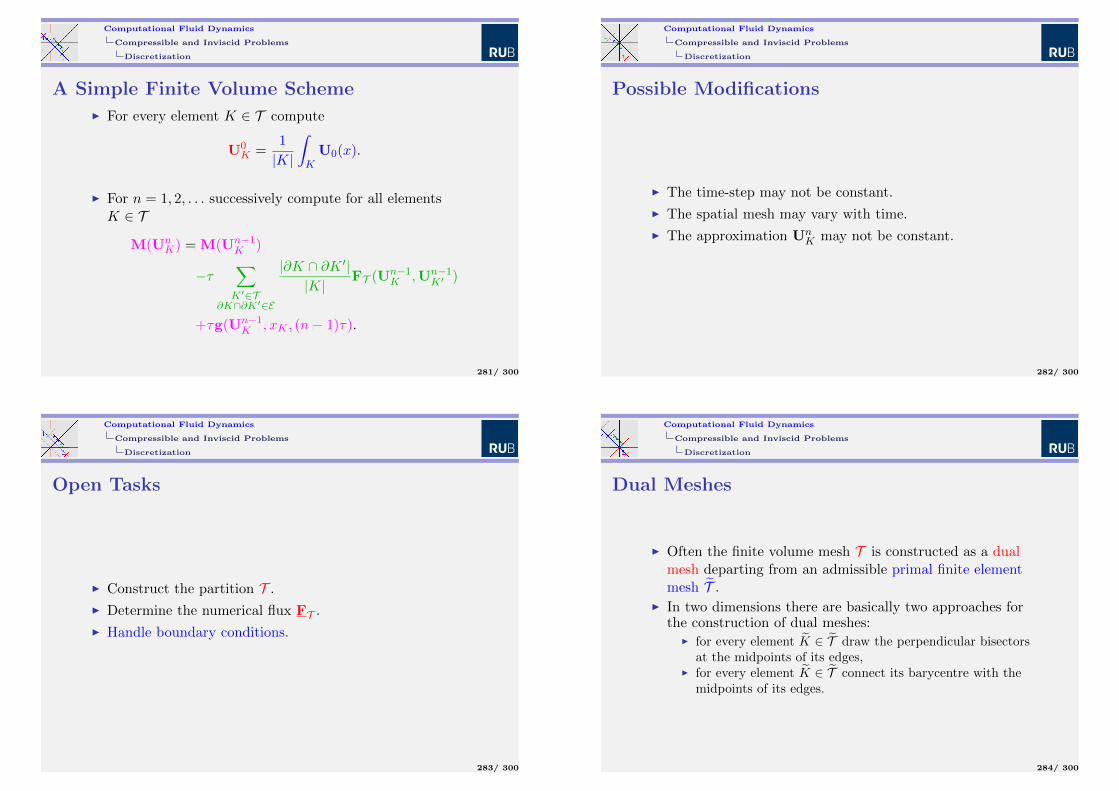
Computational Fluid Dynamics
Compressible and Inviscid Problems
Discretization
A Simple Finite Volume Scheme
I For every element K ∈ T compute
U0K =
1
|K|
∫KU0(x).
I For n = 1, 2, . . . successively compute for all elementsK ∈ T
M(UnK) = M(Un−1
K )
−τ∑K′∈T
∂K∩∂K′∈E
|∂K ∩ ∂K ′||K|
FT (Un−1K ,Un−1
K′ )
+τg(Un−1K , xK , (n− 1)τ).
281/ 300
Computational Fluid Dynamics
Compressible and Inviscid Problems
Discretization
Possible Modifications
I The time-step may not be constant.
I The spatial mesh may vary with time.
I The approximation UnK may not be constant.
282/ 300
Computational Fluid Dynamics
Compressible and Inviscid Problems
Discretization
Open Tasks
I Construct the partition T .
I Determine the numerical flux FT .
I Handle boundary conditions.
283/ 300
Computational Fluid Dynamics
Compressible and Inviscid Problems
Discretization
Dual Meshes
I Often the finite volume mesh T is constructed as a dualmesh departing from an admissible primal finite elementmesh T .
I In two dimensions there are basically two approaches forthe construction of dual meshes:
I for every element K ∈ T draw the perpendicular bisectorsat the midpoints of its edges,
I for every element K ∈ T connect its barycentre with themidpoints of its edges.
284/ 300
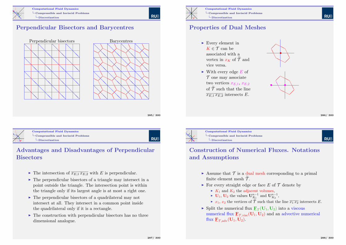
Computational Fluid Dynamics
Compressible and Inviscid Problems
Discretization
Perpendicular Bisectors and Barycentres
Perpendicular bisectors
@@@@
@@@@
@@@@
@@@@
@@@@
@@@@
@@@@
@@@@
@@@@
@@@@
@@@@
@@@@
@@@@
@@@@
@@@@
@@@@
Barycentres
@@@@
@@@@
@@@@
@@@@
@@@@
@@@@
@@@@
@@@@
@@@@
@@@@
@@@@
@@@@
@@@@
@@@@
@@@@
@@@@
AA AA AA AA
AAA
AAA
AAA
AAA
AAA
AAA
AAA
AAA
AAA
AAA
AAA
AAA
AA AA AA AA
HH
HH
HH
HH
HHH
HHH
HHH
HHH
HHH
HHH
HHH
HHH
HHH
HHH
HHH
HHH
HH
HH
HH
HH
285/ 300
Computational Fluid Dynamics
Compressible and Inviscid Problems
Discretization
Properties of Dual Meshes
I Every element inK ∈ T can beassociated with avertex in xK of T andvice versa.
I With every edge E ofT one may associatetwo vertices xE,1, xE,2of T such that the linexE,1 xE,2 intersects E.
HHH
AAAHH
HAAA •
HHH
AAAH
HHAAA ••
286/ 300
Computational Fluid Dynamics
Compressible and Inviscid Problems
Discretization
Advantages and Disadvantages of PerpendicularBisectors
I The intersection of xE,1 xE,2 with E is perpendicular.
I The perpendicular bisectors of a triangle may intersect in apoint outside the triangle. The intersection point is withinthe triangle only if its largest angle is at most a right one.
I The perpendicular bisectors of a quadrilateral may notintersect at all. They intersect in a common point insidethe quadrilateral only if it is a rectangle.
I The construction with perpendicular bisectors has no threedimensional analogue.
287/ 300
Computational Fluid Dynamics
Compressible and Inviscid Problems
Discretization
Construction of Numerical Fluxes. Notationsand Assumptions
I Assume that T is a dual mesh corresponding to a primalfinite element mesh T .
I For every straight edge or face E of T denote byI K1 and K2 the adjacent volumes,I U1, U2 the values Un−1
K1and Un−1
K2,
I x1, x2 the vertices of T such that the line x1 x2 intersects E.
I Split the numerical flux FT (U1,U2) into a viscousnumerical flux FT ,visc(U1,U2) and an advective numericalflux FT ,adv(U1,U2).
288/ 300
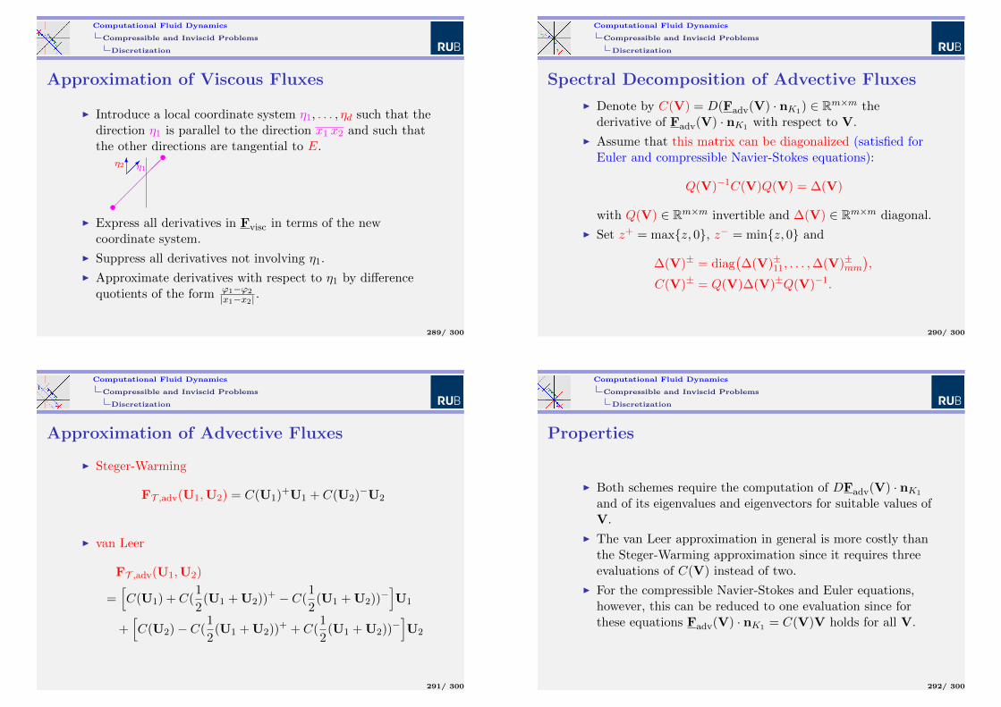
Computational Fluid Dynamics
Compressible and Inviscid Problems
Discretization
Approximation of Viscous Fluxes
I Introduce a local coordinate system η1, . . . , ηd such that thedirection η1 is parallel to the direction x1 x2 and such thatthe other directions are tangential to E.
•
•η1
η26
I Express all derivatives in Fvisc in terms of the newcoordinate system.
I Suppress all derivatives not involving η1.
I Approximate derivatives with respect to η1 by differencequotients of the form ϕ1−ϕ2
|x1−x2| .
289/ 300
Computational Fluid Dynamics
Compressible and Inviscid Problems
Discretization
Spectral Decomposition of Advective Fluxes
I Denote by C(V) = D(Fadv(V) · nK1) ∈ Rm×m thederivative of Fadv(V) · nK1 with respect to V.
I Assume that this matrix can be diagonalized (satisfied forEuler and compressible Navier-Stokes equations):
Q(V)−1C(V)Q(V) = ∆(V)
with Q(V) ∈ Rm×m invertible and ∆(V) ∈ Rm×m diagonal.
I Set z+ = maxz, 0, z− = minz, 0 and
∆(V)± = diag(∆(V)±11, . . . ,∆(V)±mm
),
C(V)± = Q(V)∆(V)±Q(V)−1.
290/ 300
Computational Fluid Dynamics
Compressible and Inviscid Problems
Discretization
Approximation of Advective Fluxes
I Steger-Warming
FT ,adv(U1,U2) = C(U1)+U1 + C(U2)−U2
I van Leer
FT ,adv(U1,U2)
=[C(U1) + C(
1
2(U1 + U2))+ − C(
1
2(U1 + U2))−
]U1
+[C(U2)− C(
1
2(U1 + U2))+ + C(
1
2(U1 + U2))−
]U2
291/ 300
Computational Fluid Dynamics
Compressible and Inviscid Problems
Discretization
Properties
I Both schemes require the computation of DFadv(V) · nK1
and of its eigenvalues and eigenvectors for suitable values ofV.
I The van Leer approximation in general is more costly thanthe Steger-Warming approximation since it requires threeevaluations of C(V) instead of two.
I For the compressible Navier-Stokes and Euler equations,however, this can be reduced to one evaluation since forthese equations Fadv(V) · nK1 = C(V)V holds for all V.
292/ 300
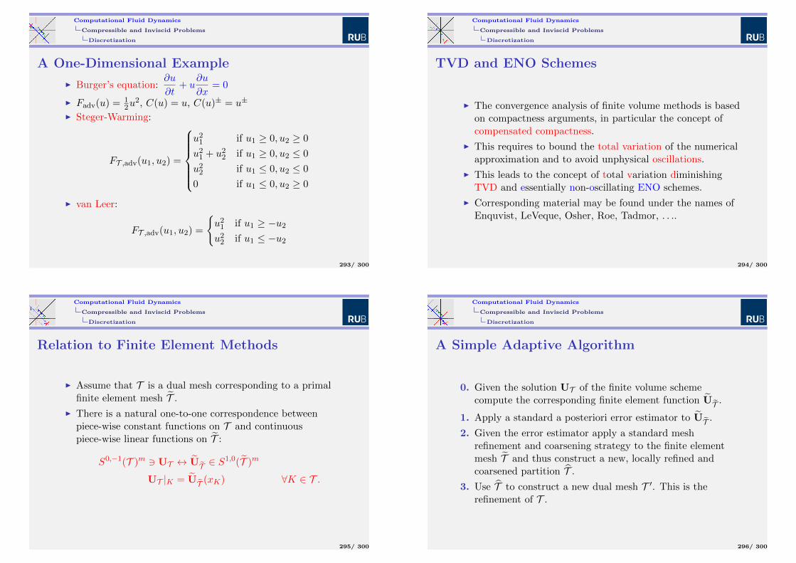
Computational Fluid Dynamics
Compressible and Inviscid Problems
Discretization
A One-Dimensional Example
I Burger’s equation:∂u
∂t+ u
∂u
∂x= 0
I Fadv(u) = 12u
2, C(u) = u, C(u)± = u±
I Steger-Warming:
FT ,adv(u1, u2) =
u2
1 if u1 ≥ 0, u2 ≥ 0
u21 + u2
2 if u1 ≥ 0, u2 ≤ 0
u22 if u1 ≤ 0, u2 ≤ 0
0 if u1 ≤ 0, u2 ≥ 0
I van Leer:
FT ,adv(u1, u2) =
u2
1 if u1 ≥ −u2
u22 if u1 ≤ −u2
293/ 300
Computational Fluid Dynamics
Compressible and Inviscid Problems
Discretization
TVD and ENO Schemes
I The convergence analysis of finite volume methods is basedon compactness arguments, in particular the concept ofcompensated compactness.
I This requires to bound the total variation of the numericalapproximation and to avoid unphysical oscillations.
I This leads to the concept of total variation diminishingTVD and essentially non-oscillating ENO schemes.
I Corresponding material may be found under the names ofEnquvist, LeVeque, Osher, Roe, Tadmor, . . ..
294/ 300
Computational Fluid Dynamics
Compressible and Inviscid Problems
Discretization
Relation to Finite Element Methods
I Assume that T is a dual mesh corresponding to a primalfinite element mesh T .
I There is a natural one-to-one correspondence betweenpiece-wise constant functions on T and continuouspiece-wise linear functions on T :
S0,−1(T )m 3 UT ↔ UT ∈ S1,0(T )m
UT |K = UT (xK) ∀K ∈ T .
295/ 300
Computational Fluid Dynamics
Compressible and Inviscid Problems
Discretization
A Simple Adaptive Algorithm
0. Given the solution UT of the finite volume schemecompute the corresponding finite element function UT .
1. Apply a standard a posteriori error estimator to UT .
2. Given the error estimator apply a standard meshrefinement and coarsening strategy to the finite elementmesh T and thus construct a new, locally refined andcoarsened partition T .
3. Use T to construct a new dual mesh T ′. This is therefinement of T .
296/ 300
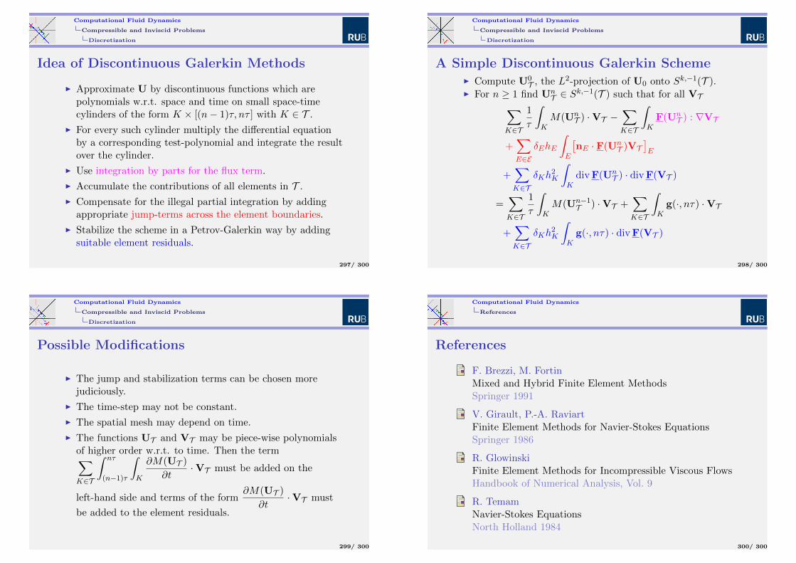
Computational Fluid Dynamics
Compressible and Inviscid Problems
Discretization
Idea of Discontinuous Galerkin Methods
I Approximate U by discontinuous functions which arepolynomials w.r.t. space and time on small space-timecylinders of the form K × [(n− 1)τ, nτ ] with K ∈ T .
I For every such cylinder multiply the differential equationby a corresponding test-polynomial and integrate the resultover the cylinder.
I Use integration by parts for the flux term.
I Accumulate the contributions of all elements in T .
I Compensate for the illegal partial integration by addingappropriate jump-terms across the element boundaries.
I Stabilize the scheme in a Petrov-Galerkin way by addingsuitable element residuals.
297/ 300
Computational Fluid Dynamics
Compressible and Inviscid Problems
Discretization
A Simple Discontinuous Galerkin SchemeI Compute U0
T , the L2-projection of U0 onto Sk,−1(T ).I For n ≥ 1 find Un
T ∈ Sk,−1(T ) such that for all VT∑K∈T
1
τ
∫KM(Un
T ) ·VT −∑K∈T
∫KF(Un
T ) : ∇VT
+∑E∈E
δEhE
∫E
[nE · F(Un
T )VT]E
+∑K∈T
δKh2K
∫K
divF(UnT ) · divF(VT )
=∑K∈T
1
τ
∫KM(Un−1
T ) ·VT +∑K∈T
∫Kg(·, nτ) ·VT
+∑K∈T
δKh2K
∫Kg(·, nτ) · divF(VT )
298/ 300
Computational Fluid Dynamics
Compressible and Inviscid Problems
Discretization
Possible Modifications
I The jump and stabilization terms can be chosen morejudiciously.
I The time-step may not be constant.
I The spatial mesh may depend on time.
I The functions UT and VT may be piece-wise polynomialsof higher order w.r.t. to time. Then the term∑K∈T
∫ nτ
(n−1)τ
∫K
∂M(UT )
∂t·VT must be added on the
left-hand side and terms of the form∂M(UT )
∂t·VT must
be added to the element residuals.
299/ 300
Computational Fluid Dynamics
References
References
F. Brezzi, M. FortinMixed and Hybrid Finite Element MethodsSpringer 1991
V. Girault, P.-A. RaviartFinite Element Methods for Navier-Stokes EquationsSpringer 1986
R. GlowinskiFinite Element Methods for Incompressible Viscous FlowsHandbook of Numerical Analysis, Vol. 9
R. TemamNavier-Stokes EquationsNorth Holland 1984
300/ 300