Definition and Implementation of Voltage Stability

Indices in PSS®NETOMAC Master of Science Thesis in Electric Power Engineering

MINH TUAN TRAN

Department of Energy and Environment

Division of Electric Power Engineering CHALMERS UNIVERSITY OF TECHNOLOGY

Göteborg, Sweden, 2009

Definition and Implementation of Voltage Stability

Indices in PSS®NETOMAC

MINH TUAN TRAN

Conducted at Siemens AG

E D SE PTI NC

Erlangen, Germany

Supervisor: Dr. Edwin Lerch

Examiner: Dr. Tuan Anh Le

Department of Energy and Environment Division of Electric Power Engineering

CHALMERS UNIVERSITY OF TECHNOLOGY

Göteborg, Sweden 2009

Definition and Implementation of Voltage Stability Indices in

PSS®NETOMAC

MINH TUAN TRAN

© MINH TUAN TRAN, 2009.

Department of Energy and Environment

Chalmers University of Technology SE-412 96 Göteborg

Sweden

Telephone + 46 (0)31-772 1000

Göteborg, Sweden 2009

Acknowledgement

I would like to express my thanks to the Swedish Institute, who has given me financial supports

during the master program in Sweden.

I am bound to thank my examiner, Dr. Tuan A. Le in Chalmers University of Technology, who has

inspired me with his classes and supported me in this thesis topic.

The thesis work is conducted in Siemens AG, Power Technology International, in Erlangen. I am

deeply indebted to my supervisor, Dr. Edwin Lerch whose ideals, continuous suggestions and

guidance helps me complete the thesis.

My special thanks go to Msc. Tuan N. Trinh, my colleague and dear friend. He has given me valuable

supports and encouragements during the time I am doing the thesis.

I also would like to express my thanks to all friends, colleagues in Erlangen, and Göteborg who have

given me cheering time and exciting life during the time I am far from home.

Last but not least, I would like to express my gratitude to my family whose patient love enable me to

complete this work.

Abstract

This thesis discusses important aspects related to voltage stability indices and their uses in

electric power system analysis and operation. Some indices previously studied in the

literature are reviewed and implemented in a reduced local network such as Line Stability

Index (Lmn), Voltage Collapse Prediction Index (VCPI), and Power Transfer Stability Index

(PTSI). In this thesis, a new index, Approximate Collapse Power Index (ACPI), is proposed

based on quadratic approximation of PV-curves. All indices are calculated and compared

with the existing Siemens‟s voltage stability criteria, Local Load Index (LLI) and Phase

Angle Index (PAI), derived for the reduced local network. The performances of the indices

are investigated for both steady-state and dynamic analyses through the IEEE 9-bus test

system and a larger test network including 119 generators and 414 nodes using Power System

Simulator and Network Torsion Machine Control (PSS®NETOMAC) software. A

comparison of the indices regarding to sensitivities, and calculation time has been done. The

results show that the performances of these indices are corresponding to one another

regarding to voltage stability of the power system. All indices were found falling between 0

and 1 in their intended range. When the system is stable, these indices are closed 0. When the

system is in critical condition with regard to voltage instability, the indices moved towards

closed to 1, but at different levels of convergence to 1. The Siemens‟s voltage stability

criteria were found less sensitive compared to other indices in the study. They, however, have

advantages of shorter calculation time, especially PAI. The proposed ACPI index was found

the most sensitive one towards voltage instability. However, ACPI index requires the longest

computational time. The ACPI index is recommended to be implemented in the voltage

stability assessment module in PSS®NETOMAC.

Key words: Voltage stability, voltage stability indices, P-V curves, dynamic simulations.

1/66

Table of Contents

Acknowledgement ............................................................................................................................. I

Abstract II

Table of Contents .............................................................................................................................. 1

List of Abbreviations ........................................................................................................................ 3

List of Figures ................................................................................................................................... 4

List of Tables ..................................................................................................................................... 6

1 Introduction .................................................................................................................. 7

2 Voltage Stability .......................................................................................................... 10

2.1 Concept and classification of voltage stability ............................................................... 10

2.2 Analysis of voltage stability .......................................................................................... 10

2.2.1 Single load, infinite bus system ..................................................................................... 10

2.2.2 Voltage stability analysis in nonlinear power systems .................................................... 12

2.2.2.1 Dynamic analysis .......................................................................................................... 12

2.2.2.2 Static analysis ............................................................................................................... 12

2.2.2.2.1. Steady-state stability ..................................................................................................... 12

2.2.2.2.2. Load flow feasibility ..................................................................................................... 13

2.2.3 Introduction of simulation software PSS®NETOMAC .................................................. 14

3 Voltage Stability Indices ............................................................................................. 16

3.1 Loading margin ............................................................................................................. 16

3.2 Line stability index ........................................................................................................ 18

3.3 Voltage collapse prediction index .................................................................................. 18

3.4 Power transfer stability index ........................................................................................ 19

4 Formulation of Voltage Stability Indices .................................................................... 21

4.1 Reduced local network .................................................................................................. 21

4.2 Formulation of voltage stability indices ......................................................................... 22

4.2.1 Siemens specific formulation of stability criteria ........................................................... 22

4.2.2 Approximate collapse power index ................................................................................ 23

4.2.3 Applying of previous indices in the reduced local network ............................................ 24

2/66

4.2.4 Calculating the indices in PSS®NETOMAC ................................................................. 25

5 Simulation Results and Discussions ............................................................................ 27

5.1 9 bus system test ........................................................................................................... 27

5.1.1 Description of the 9 bus test system ............................................................................... 27

5.1.2 Static analysis ............................................................................................................... 28

5.1.2.1 Case 1 without limitation of reactive power generators .................................................. 28

5.1.2.2 Case 2 including reactive power generator limitations ................................................... 30

5.1.2.3 Remarks of static tests ................................................................................................... 33

5.1.3 Dynamic analysis .......................................................................................................... 33

5.1.3.1 Effects of AVR and OXL .............................................................................................. 33

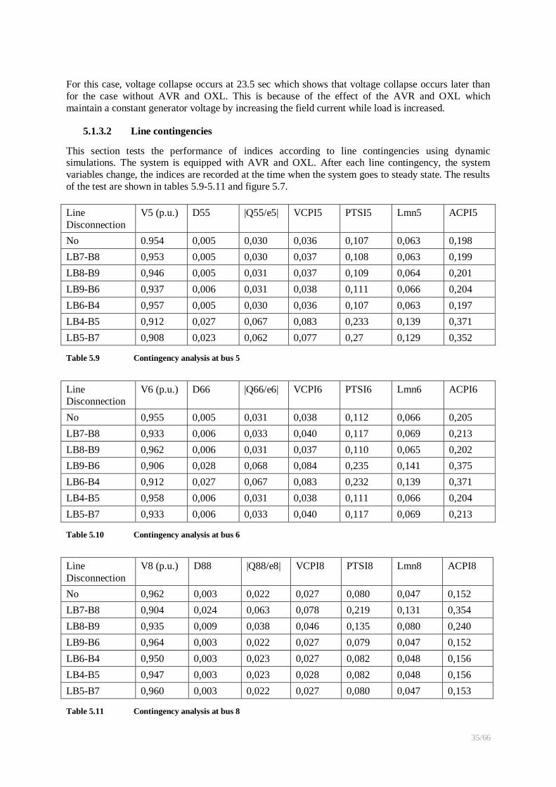
5.1.3.2 Line contingencies ........................................................................................................ 35

5.1.3.3 Remarks of the dynamic tests ........................................................................................ 37

5.2 Larger network test ....................................................................................................... 37

5.2.1 Description of the larger test network ............................................................................ 37

5.2.2 Load increasing ............................................................................................................. 37

5.2.3 Disconnection of transmission lines ............................................................................... 39

5.2.4 Time of calculations ...................................................................................................... 40

5.2.5 Remarks of the larger network test ................................................................................ 42

6 Conclusion ................................................................................................................... 43

References 44

Appendix 46

3/66

List of Abbreviations

ACPI Approximate Collapse Power Index

AVR Auto Voltage Regulator

BCT Base Calculation Time

ICT Individual Calculation Time

IEEE Institute of Electrical and Electronics Engineers

LFF Load Flow Feasibility

Lmn Line Stability Index

Nc Number of Contingencies

NETOMAC Network Torsion Machine Control

OXL Over Excitation Limiter

PMU Phasor Measurement Unit

PSS Power System Simulator

PTSI Power Transfer Stability Index

PV Power Voltage

SSS Steady State Stability

Tt Total Simulation Time

VCPI Voltage Collapse Prediction Index

VS Voltage Stability

4/66

List of Figures

Figure 2.1 Single load, infinite-bus system ...................................................................... 11

Figure 2.2 PV curves for different load power factors ...................................................... 11

Figure 2.3 Possible ways of simulations ......................................................................... 15

Figure 2.4 PSS® NETOMAC as subroutines for identification and optimization ............. 15

Figure 3.1 PV curve of a load bus in the power system .................................................... 17

Figure 3.2 QV curve of a load bus in the power system ................................................... 17

Figure 3.3 Single line diagram of a transmission line in the power system ....................... 18

Figure 3.4 Thevenin equivalent diagram .......................................................................... 19

Figure 4.1 Network viewed from node j (a) reduced local network (b) ............................. 21

Figure 4.2 Calculation block diagram of the indices in PSS®NETOMAC ....................... 26

Figure 5.1 9 bus- 3 generator- test network ...................................................................... 27

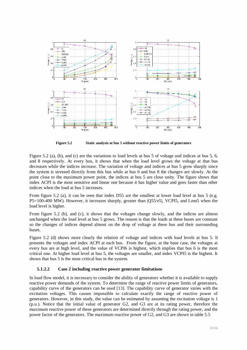
Figure 5.2 Static analysis at bus 5 without reactive power limits of generators ................. 30

Figure 5.3 Static analysis considering reactive power limits of generators........................ 32

Figure 5.4 Static analysis of bus 5 at two cases ................................................................ 32

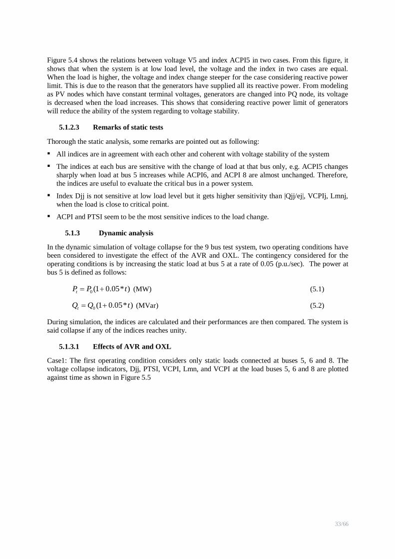
Figure 5.5 Dynamic simulations without considering AVR and OXL .............................. 34

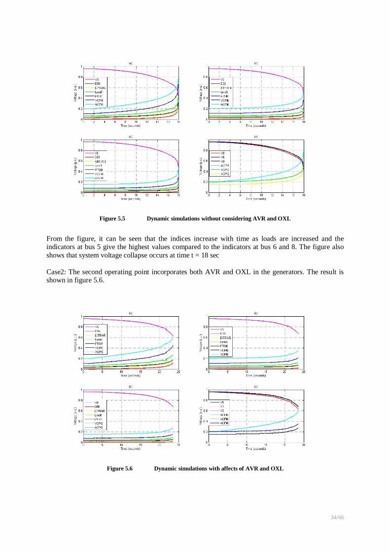
Figure 5.6 Dynamic simulations with affects of AVR and OXL ....................................... 34

Figure 5.7 Line contingencies and index performances .................................................... 36

Figure 5.9 Local network of bus SRT___00 .................................................................... 38

Figure 5.10 Load increasing at bus SRT_00 ...................................................................... 39

Figure 5.11 Line contingencies in the larger test network .................................................. 39

Figure 5.12 Disconnection of transmission lines in the larger test network ......................... 40

Figure 5.13 Calculation time of an index in a variant calculation ....................................... 41

Figure 5.14 Total simulation time and its fractions ............................................................ 42

Figure A.1 The reduced local network .............................................................................. 47

Figure A.2 Excitation system type AC2A- [23] ................................................................ 49

Figure A.3 Larger test network overview [21] .................................................................. 51

Figure A.4 Contingency locations [21] ............................................................................. 52

Figure A.5 Block diagrams of AVRs used in the larger test network [21] ......................... 53

Figure A.6 Parameter setting of AVRs used in the larger test network [21] ....................... 54

Figure A.7 Block diagrams of governors used in the larger test network [21] .................... 55

Figure A.8 Parameter setting of governors used in the larger test network [21] ................. 56

5/66

Figure A.9 Variation of the total simulation time to integration time step ......................... 57

Figure A.10 Variation of the total simulation time to the number of contingencies ............. 57

Figure A.11 Macro calculating branch admittance Yij.mac ................................................. 58

Figure A.12 Macro calculating the self admittance Yjj.mac (cont) ..................................... 59

Figure A.13 Macro calculating the self admittance Yjj.mac ................................................ 60

Figure A.14 Macro calculating index Djj Djj_index.mac .................................................... 61

Figure A.15 9 bus network static analysis without considering reactive power limits .......... 62

Figure A.16 9 bus network static analysis considering reactive power limits ....................... 63

Figure A.17 9 bus network line contingency analysis ......................................................... 64

Figure A.18 9 bus network dynamic analysis without considering AVR and OXL .............. 65

Figure A.19 9 bus network dynamic analysis considering AVR and OXL .......................... 65

Figure A.20 Larger test network, load increasing at bus SRT___00 .................................... 66

Figure A.21 Disconnection of transmission lines in the larger test network ......................... 66

6/66

List of Tables

Table 5.1 9 bus test network setting at base load level .................................................... 28

Table 5.2 Static analysis at bus 5 without considering reactive power limits of generators29

Table 5.3 Static analysis at bus 6 without considering reactive power limits of generators29

Table 5.4 Static analysis at bus 8 without considering reactive power limits of generators29

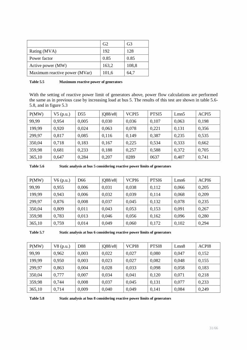
Table 5.5 Maximum reactive power of generators .......................................................... 31

Table 5.6 Static analysis at bus 5 considering reactive power limits of generators ........... 31

Table 5.7 Static analysis at bus 6 considering reactive power limits of generators ........... 31

Table 5.8 Static analysis at bus 8 considering reactive power limits of generators ........... 31

Table 5.9 Contingency analysis at bus 5 ......................................................................... 35

Table 5.10 Contingency analysis at bus 6 ......................................................................... 35

Table 5.11 Contingency analysis at bus 8 ......................................................................... 35

Table 5.12 Line contingency ranking with index ACPI .................................................... 36

Table 5.13 Sensitivity comparison of the indices .............................................................. 37

Table 5.14 Index performance according to line contingencies ......................................... 40

Table 5.15 Comparison of the calculation time of indices ................................................. 42

Table 6.1 Comparison of the indices .............................................................................. 43

Table A.1 Synchronous machine parameters ................................................................... 48

Table A.2 Transmission line parameters ......................................................................... 48

Table A.3 Transformer parameters .................................................................................. 49

Table A.4 Parameter setting of exciter type IEEE CA2A (a) ........................................... 49

Table A.5 Parameter setting of exciter type IEEE CA2A (b) ........................................... 50

7/66

1 Introduction

Recently, several blackouts are reported in many countries relate to voltage stability problems.

There are 6 blackouts within 6 weeks in 2003 affecting about 112 million people in US, UK,

Denmark, and Sweden [1]. These accidents are due to several common features. They had no

problems with generation adequacy, however, all transmission-based. Power systems are operating under increasing stresses. Loads are increasing while transmission networks are not adequately

enlarged since economic and environmental restrictions. The power systems are interconnected

and they are operated with higher power transfers between areas while there is little coordination and exchange of on-line information between utilities. In essence, the direct cause of blackouts has

been found is voltage collapse.

Generally, voltage collapse is the process by which the sequence of events accompanying voltage instability leads to a low unacceptable voltage profile in a significant part of the power system [2].

In power systems, reactive power is needed to support magnetic fields of inductors and electric

fields of capacitors in generic loads. The reactive power can be supplied by generators through transmission networks, or compensated directly at load buses by compensators such as shunt

capacitors, and synchronous condensers. There are two side effects of reactive power transmission

those are transmission losses and voltage drops. When the load voltage is lower, both the transmission losses and voltage drops are higher, which cause the voltage at the load bus more

decreased. The voltage constraints prevent long distant transfer of reactive power and the lack of

reactive power will directly relate to voltage collapse. It normally follows by a disturbance in the

power system. After a disturbance, there is a sudden increase of reactive power demand. If the demand is not met, the disturbance leads to voltage collapse, causing a major breakdown of part or

all of the system.

Voltage collapse may be a possible outcome of voltage instability, which is defined as the attempt

of load dynamics to restore power consumption beyond the capability of the combined

transmission and generation system. [2]. Voltage instability of radial distribution systems has been

recognized and understood. It was often referred to as load instability. It may be assessed by the

relationship between the voltage and reactive power balance at a load bus. For example if reactive

power demand is assumed constant, when the voltage decreases and reactive power supply increase, it is stable. Vice versa, if the voltage decreases together with the reactive power supply it

is instable.

There are many affects relating to voltage instability such as dynamic loads, reactive power generations, load tap changer transformers and power transfer capability of transmission systems.

Most of these factors have a significant effect on reactive power production, consumption and

transmission. Switching of shunt capacitors, blocking of tap-changing transformers, dispatching of generations, rescheduling of generators, secondary voltage regulations, and load shedding, are

some of counteractions against voltage collapse.

Researches interested in voltage instability examine two aspects: proximity to voltage instability

and mechanism to voltage instability. The first aspect is to determine the current status of power

system and estimate the distance to voltage instability by means of physical quantities. The second

aspect finds out the reason, contributing factors, involving areas of voltage instability. Proximity

8/66

gives a measure of voltage security while mechanism provides information useful in determining

activities or operating strategies which could be used to prevent voltage instability [3]

Analysis of voltage instability may be categorized into static and dynamic approaches. In dynamic

analysis, all elements of the network are modeled by means of algebraic and differential equations.

The study of the power system is done through time domain simulations. The approach requires a

lot of computations as well as calculation time. Furthermore, it does not provide readily sensitivity information or the degree of voltage instability. However, it can reflex accurately the mechanism

of voltage instability, which in reality a dynamic phenomenon.

The static analysis can be subdivided into Load Flow Feasibility (LFF) and Steady-state Stability

(SSS) approaches. These approaches are used to calculate the voltage collapse criteria of the

power system. LFF is related to the existence of an acceptable voltage profile across the network

based on solving conventional power flow. It is concerned with the maximum power transfer capability of the network or the existence of a solved load flow case based on evaluating the

singularity of load flow Jacobian matrix. SSS approach is concerned with the existence of a stable

operating point of the power system modeled by algebraic and differential equations. The steady state Jacobian matrix is obtained by solving the set of equations which is linearized around the

operating point. This approach evaluates the singularity of the steady state Jacobian matrix to

determine the maximum loadability of the power system including affects of generators and other voltage dependent devices [4].

In voltage stability analysis, it is useful to assess voltage stability of power systems by means of

scalar magnitudes, or indices. Operators can use voltage stability indices to know how close the system to voltage collapse. These indices may be use on-line or off-line to help operators in real

time operation of power system or in designing and planning operations. In literature many static

voltage assessment techniques have been proposed, such as the minimum singularity value, mode analysis and sensitivity method [5-7]. The main disadvantages of these techniques include

considerable computational efforts making implementation difficult in on-line applications.

Voltage instability often starts in a local network and gradually extends to the whole system. This

feature enables to predict static voltage stability using local measurements. There are two types of

local evaluation techniques for voltage stability: line-based and node (bus)-based techniques.

Conceptually, if a line or a node in the system is critically voltage-instable, the whole system approaches a collapse point [8-11].

The aim of the thesis is to find a voltage stability index which is applicable to be implemented in power system tool PSS®NETOMAC, which is developing by Siemens. The approach of study is

to investigate voltage problem of the power system under the feasible solution of load flows of a

reduced local network. The voltage stability will be evaluated at each nodes in the system based

on the voltages of the node and its surrounding nodes, and the line admittances. In this thesis, some techniques which are based on local phasor measurement will be applied into the reduced

local network such as Voltage Collapse Prediction Index (VCPI), Power Transfer Stability Index

(PTSI). Line Stability Index (Lmn). Besides, a new index, Approximate Collapse Power Index (ACPI) based on quadratic approximation of PV- curves is proposed. These indices then are

compared with Siemens specific voltage stability criteria, Local Load Index (LLI), and Phase

Angle Index (PAI) regarding to sensitivities and calculation time. The performances of these indices are verified through static and dynamic analysis of a 9 bus test system and a larger test

network including 414 buses and 119 generators.

The analyses presented in this thesis are developed using the software tool and acknowledgments from Siemens AG, Power Technology International (Siemens PTI) department in Erlangen,

Germany. The contribution of this work for the company involves the necessity to implement a

9/66

meaningful voltage stability index in a voltage stability module in power system simulator

PSS®NETOMAC.

The structure of the thesis is as followings:

- Chapter 1 ( this chapter) gives backgrounds and objectives of the thesis

- Chapter 2 introduces definitions of voltage stability, the approach to study voltage stability.

Infinite-bus system is introduced to evaporate the basic concept in voltage stability. A short description of simulation tool PSS®NETTOMAC is presented.

- Chapter 3 reviews some earlier indices of voltage stability including PV, and QV curve, some

indices based on different deriving methods refer to local phasor measurements. - Chapter 4 introduces a reduced local network. Siemens voltage criteria and a new voltage

stability index are derived. Indices reviewed in chapter 2 are implemented in the local

network. This section also sets up calculating the indices in PSS®NETOMAC

- Chapter 5 investigates the performance of the indices in test networks. The study is conducted in both static and dynamic approaches with different scenarios. Performance of the indices

regarding to sensitivities, and calculation time are compared.

- Chapter 6 summaries the performance of the indices and give some discussions and conclusions.

10/66

2 Voltage Stability

Voltage stability is a problem in power system which is lack of reactive power support when heavily

loaded or the network transfer capability is reduced due to disturbances. The problem of voltage stability concerns the whole power system, although it usually has a large involvement in one critical

area of the power system.

This chapter describes some basic concepts of voltage stability. First voltage stability, voltage instability and voltage collapse are defined. Infinite-bus system is introduced to present PV curve and

maximum power transfer. Then different methods of voltage stability analysis are briefly introduced.

A short introduction of simulation tool PSS®NETOMAC is presented.

2.1 Concept and classification of voltage stability

Beside rotor angle stability, or transient stability, power system stability also concerns to voltage

stability. In [12], the voltage stability is defined as follows: “The voltage stability is the ability of a

power system to maintain steady acceptable voltages at all buses in the system at normal operating

conditions and after being subjected to a disturbance.”

According to [2] the definition of voltage instability is “Voltage instability stems from the attempt of

load dynamics to restore power consumption beyond the capability of the combined transmission and generation system.”

Voltage instability may, or may not lead to voltage collapse, which is defined by [2] as the catastrophic result of a sequence of events leading to a low-voltage profile suddenly in a major part of

the power system. When lacking of the reactive power transfer capability to the load, the power

system may cause voltage instability. Therefore, any changes in the power system which affects the

reactive power transfer such as dynamic loads, reactive power generation, disconnection of transmission lines, or switching off static compensators are factors relating to voltage instability.

Classification of voltage stability helps analysis the problem, and identifies factors relating to voltage instability. Depending on time scale, Voltage stability is classified as short term and long term voltage

stability. Short term voltage stability involves dynamics of fast acting load components like induction

motors, electronically controller loads. The study period of interest is in order of several seconds.

While long term voltage stability refers to slower acting equipments like tap changing transformers, generator current limiters. The study period of interest extends to several minutes [12]

2.2 Analysis of voltage stability

2.2.1 Single load, infinite bus system

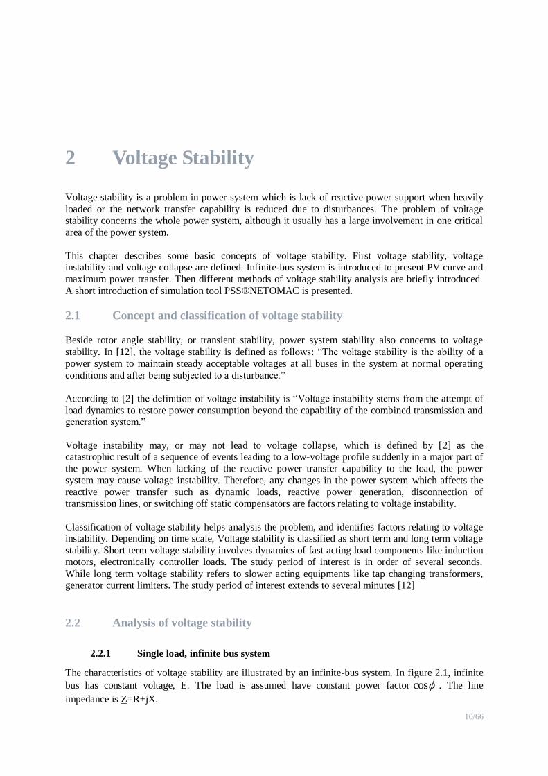
The characteristics of voltage stability are illustrated by an infinite-bus system. In figure 2.1, infinite

bus has constant voltage, E. The load is assumed have constant power factor cos . The line

impedance is Z=R+jX.

11/66

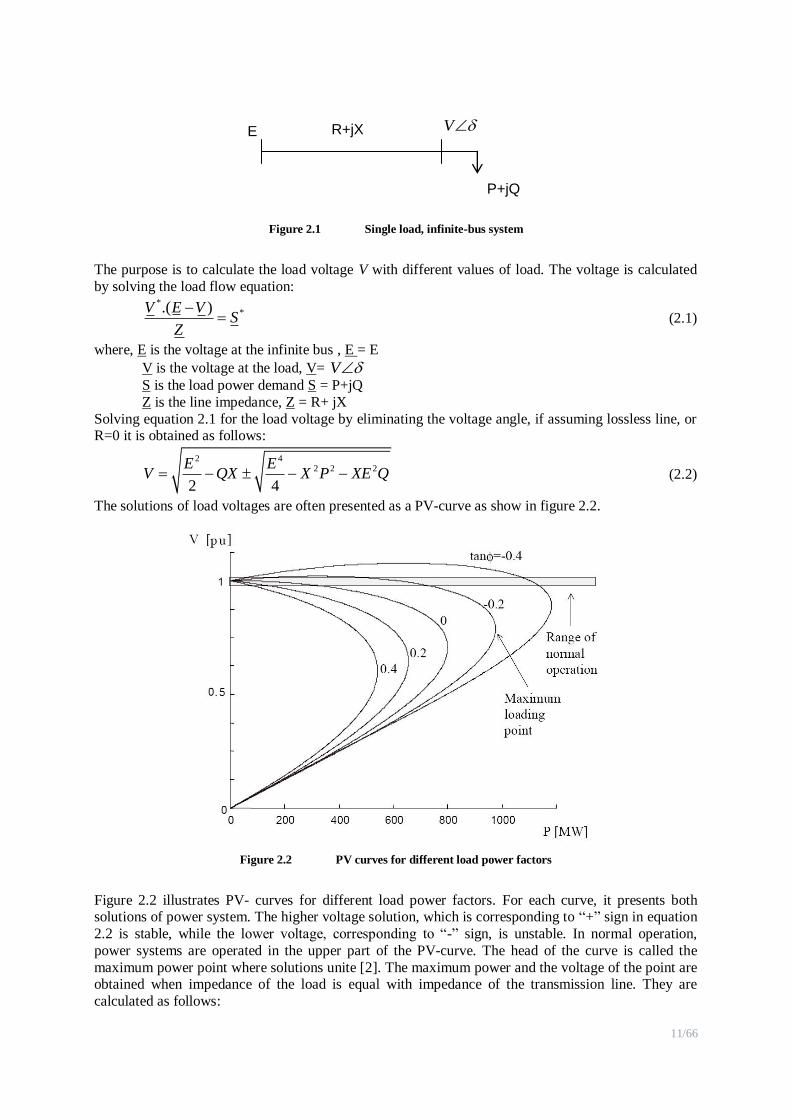
Figure 2.1 Single load, infinite-bus system

The purpose is to calculate the load voltage V with different values of load. The voltage is calculated

by solving the load flow equation: *

*.( )V E VS

Z

(2.1)

where, E is the voltage at the infinite bus , E = E

V is the voltage at the load, V= V

S is the load power demand S = P+jQ

Z is the line impedance, Z = R+ jX

Solving equation 2.1 for the load voltage by eliminating the voltage angle, if assuming lossless line, or R=0 it is obtained as follows:

2 42 2 2

2 4

E EV QX X P XE Q (2.2)

The solutions of load voltages are often presented as a PV-curve as show in figure 2.2.

Figure 2.2 PV curves for different load power factors

Figure 2.2 illustrates PV- curves for different load power factors. For each curve, it presents both solutions of power system. The higher voltage solution, which is corresponding to “+” sign in equation

2.2 is stable, while the lower voltage, corresponding to “-” sign, is unstable. In normal operation,

power systems are operated in the upper part of the PV-curve. The head of the curve is called the

maximum power point where solutions unite [2]. The maximum power and the voltage of the point are obtained when impedance of the load is equal with impedance of the transmission line. They are

calculated as follows:

V E

P+jQ

R+jX

12/66

2

max

cos

1 sin 2

EP

X

(2.3)

max2 1 sin

P

EV

(2.4)

where, cos is the load power factor which can be calculated as:

2 2cos

P

P Q

(2.5)

PV-curves play a major role in understanding and explaining voltage stability. From a PV curve, the

variation of bus voltages with load, distance to instability (VS margin) and critical voltage at which instability occurs may be determined [13]

2.2.2 Voltage stability analysis in nonlinear power systems

Voltage instability is a dynamic phenomenon which may involve the interaction of many devices. It

may occur in different time frames and involve different parts of the system with nonlinear behaviours

due to interaction of different elements in power systems. Analysis of voltage stability must provide information on system state, proximity to, and mechanism of instability [13]. There are two main

methods of voltage stability analysis in nonlinear power systems: dynamic analysis and static analysis.

2.2.2.1 Dynamic analysis

In dynamic analysis, all elements in a power system are modelled by algebraic and differential

equations. The behaviour of the system under different changes of the system is studied through time domain simulations. The whole power system can be expressed under set of algebraic and differential

equations in general form as follows:

( , , )dx

f x y pdt

(2.6)

0 ( , , )g x y p (2.7)

with a set of know initial condition (x0,y0,p0), where: x is the state vector of the system ( e.g., generator phase angle and angular velocities, tap ratio

of on-load tap changer transformers)

y is the vector of algebraic variables (e.g., the direct and quadrature axis components of the stator currents)

p is the vector of parameter variables (e.g., load factor)

For a fix parameter p, equations (2.6), (2.7) are solved directly in time domain by using numerical

integration methods such as Euler, Range-Kutta methods [13]. Dynamic analysis can accurately replicate the actual dynamic of voltage stability, and show performance of system and individual

elements. It can also capture the event and chronology leading to voltage instability. However, this

method requires huge data information for modelling and expensive calculation efforts, while the degree of instability is not provided [3]. In practice, dynamic simulation is applied in essential studies

relating to coordination of protections and controls and short-term voltage stability analysis.

2.2.2.2 Static analysis

2.2.2.2.1. Steady-state stability

Steady-state stability approach investigates the power system around each operating point, which is

approximated by setting the time derivatives of state variables to zero, and the state variables take on

values appropriate to the operating point. Consequently, the overall system equations reduce to purely algebraic equations:

0 ( , , )f x y p (2.8)

13/66

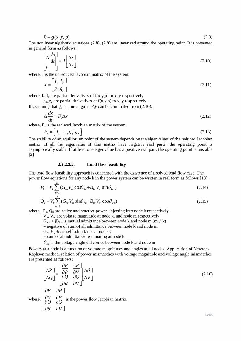
0 ( , , )g x y p (2.9)

The nonlinear algebraic equations (2.8), (2.9) are linearized around the operating point. It is presented

in general form as follows:

0

dxx

Jdty

(2.10)

where, J is the unreduced Jacobian matrix of the system:

yx

x y

ffJ

g g

(2.11)

where, fx, fy are partial derivatives of f(x,y,p) to x, y respectively

gx,,gy are partial derivatives of f(x,y,p) to x, y respectively.

If assuming that gy is non-singular y can be eliminated from (2.10):

x

dxF x

dt (2.12)

where, Fx is the reduced Jacobian matrix of the system: 1

x x y y xF f f g g (2.13)

The stability of an equilibrium point of the system depends on the eigenvalues of the reduced Jacobian

matrix. If all the eigenvalue of this matrix have negative real parts, the operating point is

asymptotically stable. If at least one eigenvalue has a positive real part, the operating point is unstable [2]

2.2.2.2.2. Load flow feasibility

The load flow feasibility approach is concerned with the existence of a solved load flow case. The

power flow equations for any node k in the power system can be written in real form as follows [13]:

)sincos(1

kmmkmkm

n

m

mkmkk VBVGVP

(2.14)

)cossin(1

kmmkmkm

n

m

mkmkk VBVGVQ

(2.15)

where, Pk, Qk are active and reactive power injecting into node k respectively

Vk, Vm are voltage magnitude at node k, and node m respectively Gkm + jBkm is mutual admittance between node k and node m (m ≠ k)

= negative of sum of all admittance between node k and node m

Gkk + jBkk is self admittance at node k = sum of all admittance terminating at node k

km is the voltage angle difference between node k and node m

Powers at a node is a function of voltage magnitudes and angles at all nodes. Application of Newton-

Raphson method, relation of power mismatches with voltage magnitude and voltage angle mismatches

are presented as follows:

V

V

QQV

PP

Q

P

(2.16)

where,

V

QQV

PP

is the power flow Jacobian matrix.

14/66

Equation (2.16) is written for all PQ nodes. For PV nodes where P and V are specified P ,

Q should be eliminated. Therefore, the Jacobian matrix would have one row and column for each

PV node.

The load flow feasibility approach determines the power system conditions for existing solutions of

equation (2.16). The method evaluates the power flow Jacobian matrix which should not be singular to

achieve a solution for power flow in the power system.

Static analysis offers several advantages. It can provide insight into state, proximity to, and

mechanism of instability. Furthermore, modelling assumption helps the calculation time reduced compared to dynamic approach. However, it does not give information if the operating point can be

reached and unable to applied in short term voltage stability. In practice, static analysis is used for

bulk of planning and operating studies where many contingencies must be analyzed. Besides, the

approach is applied in real time operation of power system where fast calculation time is necessary [3].

2.2.3 Introduction of simulation software PSS®NETOMAC

PSS®NETOMAC (Power System Simulator and Network Torsion Machine Control) is a program

researched and developed by Siemens. It performs calculations relating to electrical systems consisting of a network, machines and open-loop and closed-loop control equipments [14]. The

software has a uniform database and enables the following calculations:

▪ Simulation of electromagnetic and electro-mechanic transient phenomena in the time domain

▪ Calculation of instantaneous values with simulation of the network and machines by means of

differential equations. Calculation of stability with simulation of the network using complex

impedance and machines by means of differential equations

▪ Special calculations of load flow

▪ Frequency domain analysis

▪ Eigenvalue analyses

▪ Simulation of torsional oscillation systems

▪ Parameter identification

▪ Optimization

▪ Reduction of passive networks

With PSS® NETOMAC, differential-equation systems of electrical systems are integrated step by step.

In the analyses of both time and frequency domain as well as eigenvalue analyses, the load-flow

program can be used to determine the working point. The possible ways of simulation are shown in figure 2.3.

15/66

Figure 2.3 Possible ways of simulations

When PSS® NETOMAC is used in parameter identification and optimization it is called as a

subroutine. The relationship is shown in figure 2.4.

Figure 2.4 PSS® NETOMAC as subroutines for identification and optimization

There are some main characteristics of PSS®NETOMAC:

▪ Using only one input data file to do all calculations.

▪ Flexible uses of variables help the input data file easier to be read and modified

▪ Controller design is a very important characteristic. A block-oriented language is adopted to design

controllers.

▪ Ability to use variant calculations, which facilitate looped simulations

▪ Parameter setting of simulation data, output data can be implemented and modified online

Loadflow initial conditions Only loadflow Loadflow operating point

Network R-S-T

admittances by

differential equation

non-linearities

System component linearization

coupling

Electromagnetic and

electromechanical

phenomena, complete solution

Electromechanical

phenomena,

fundamental solution

Loadflow for

special

requirements

Small signal

characteristics

Network, machine and control

System-oscillation

and -damping,

net-reduction. Control layout

Simulation models for System components,

Machines,

Controller and control units

Single line networks

complex admittances

only fundamental

frequency

Time range

instantaneous values ns...μs...ms...s

Time range quasi

steady-state values s...min

Frequency

range all

system-

varialbes

Eigenvalue analysis

Variation of

parameters,

Selection of variants

Variation of

Fault duration

Model- structure,

Parameter-ranges

Measured values

Model- structure,

Parameter-ranges

Target function

Motor-data

Parameter-ranges

Torque characteristic

NETOMAC called as subroutine

Algorithm to identify or optimize the free parameters

Parameter studies Statistical studies

Dynamic stability limit

Parameter

identification,

Time range Frequency range

Parameter

optimization,

Time range Frequency range

Parameter

identification, in the

motor equivalent circuit

16/66

3 Voltage Stability Indices

In voltage stability analysis, it is interesting and useful to know as the system parameters change prone to voltage stability by mean of monitoring scalar magnitudes, or indices. Operators can use the indices

to know how close the system to voltage collapse, or how much power that the system can supply to

loads. These indices should be use on-line or off-line to help operators in real time operation of power system or in designing and planning operations. These indices should have a predictable shape, linear,

and sensitive with the system change relating to voltage problem so that acceptable prediction can be

made and necessary activities can be activated to mitigate the problem. Furthermore, they should be

simple, easy to implement and computationally inexpensive, particularly for on-line system monitoring [15]

The condition of voltage stability in a power system can be known using voltage stability indices. These indices may be based on static analysis or dynamic models of the power systems. They can

either reveal the critical bus of a power system or the stability of each line connected between two

buses in an interconnected network or evaluate the voltage stability margins of a system. In literature, many techniques that approximate voltage collapse based on LFF and SSS approaches have been

developed such as PV and QV curves, modal analysis [6], sensitive method [16], voltage phasor

approach [17], eigenvalue method [5]. This section reviews some voltage collapse criteria which is

capable to be applied in a reduced local network, which is introduced in section 4, and simple to be implemented in PSS®NETOMAC software.

3.1 Loading margin

Loading Margin is the most basic and widely accepted method to approximate voltage collapse in the power system. For a current operating point, the total of increment of load in a specified pattern of

load increase that would cause a voltage collapse is called the loading margin to voltage collapse. [15]

The PV and QV curves are the most used to determine the loading margin of a power system at an

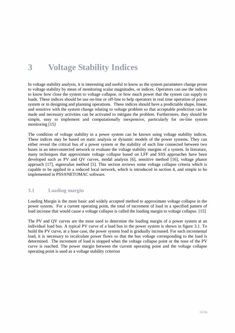
individual load bus. A typical PV curve of a load bus in the power system is shown in figure 3.1. To

build the PV curve, at a base case, the power system load is gradually increased. For each incremental

load, it is necessary to recalculate power flows so that the bus voltage corresponding to the load is determined. The increment of load is stopped when the voltage collapse point or the nose of the PV

curve is reached. The power margin between the current operating point and the voltage collapse

operating point is used as a voltage stability criterion

17/66

Figure 3.1 PV curve of a load bus in the power system

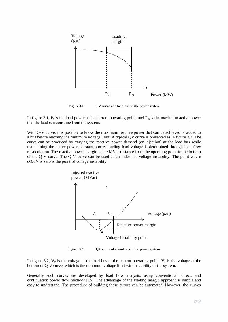
In figure 3.1, P0 is the load power at the current operating point, and Pm is the maximum active power that the load can consume from the system.

With Q-V curve, it is possible to know the maximum reactive power that can be achieved or added to a bus before reaching the minimum voltage limit. A typical QV curve is presented as in figure 3.2. The

curve can be produced by varying the reactive power demand (or injection) at the load bus while

maintaining the active power constant, corresponding load voltage is determined through load flow

recalculation. The reactive power margin is the MVar distance from the operating point to the bottom of the Q-V curve. The Q-V curve can be used as an index for voltage instability. The point where

dQ/dV is zero is the point of voltage instability.

Figure 3.2 QV curve of a load bus in the power system

In figure 3.2, V0 is the voltage at the load bus at the current operating point. Vc is the voltage at the

bottom of Q-V curve, which is the minimum voltage limit within stability of the system.

Generally such curves are developed by load flow analysis, using conventional, direct, and continuation power flow methods [15]. The advantage of the loading margin approach is simple and

easy to understand. The procedure of building these curves can be automated. However, the curves

P0 Pm

Voltage

(p.u.) Loading

margin

Power (MW)

Voltage instability point

Injected reactive

power (MVar)

Reactive power margin

Voltage (p.u.) V0 Vc

18/66

must be generated at each bus. Furthermore, it needs information of the system which is beyond the

operating point hence the cost of calculations will be very high.

3.2 Line stability index

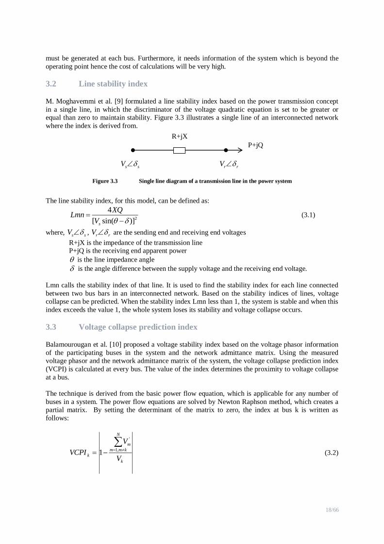
M. Moghavemmi et al. [9] formulated a line stability index based on the power transmission concept

in a single line, in which the discriminator of the voltage quadratic equation is set to be greater or equal than zero to maintain stability. Figure 3.3 illustrates a single line of an interconnected network

where the index is derived from.

Figure 3.3 Single line diagram of a transmission line in the power system

The line stability index, for this model, can be defined as:

2

4

[ sin( )]s

XQLmn

V

(3.1)

where, s sV , r rV are the sending end and receiving end voltages

R+jX is the impedance of the transmission line P+jQ is the receiving end apparent power

is the line impedance angle

is the angle difference between the supply voltage and the receiving end voltage.

Lmn calls the stability index of that line. It is used to find the stability index for each line connected

between two bus bars in an interconnected network. Based on the stability indices of lines, voltage collapse can be predicted. When the stability index Lmn less than 1, the system is stable and when this

index exceeds the value 1, the whole system loses its stability and voltage collapse occurs.

3.3 Voltage collapse prediction index

Balamourougan et al. [10] proposed a voltage stability index based on the voltage phasor information

of the participating buses in the system and the network admittance matrix. Using the measured voltage phasor and the network admittance matrix of the system, the voltage collapse prediction index

(VCPI) is calculated at every bus. The value of the index determines the proximity to voltage collapse

at a bus.

The technique is derived from the basic power flow equation, which is applicable for any number of

buses in a system. The power flow equations are solved by Newton Raphson method, which creates a partial matrix. By setting the determinant of the matrix to zero, the index at bus k is written as

follows:

k

N

kmm

m

kV

V

VCPI

,1

'

1 (3.2)

s sV r rV

R+jX

P+jQ

19/66

where, mN

kjj

kj

kmm V

Y

YV

,1

' (3.3)

Vk is the voltage phasor at bus k Vm is the voltage phasor at bus m

Ykm is the admittance between bus k and m

Ykj is the admittance between bus k and j k is the monitoring bus

m is the other bus connected to bus k

N is the bus set of the system. The value of VCPI varies between 0 and 1. If the index is zero, the voltage at bus k is considered

stable and if the index is unity, a voltage collapse is said to occur. VCPI is calculated only with

information of voltage phasor of participating buses and impedance of relating lines. The calculation is

simple without matrix conversion. The technique offers fast calculation which can be applied for online monitoring of the power system.

3.4 Power transfer stability index

Nizam et al. [18] derived the power transfer stability index (PTSI) by considering a simple two-bus

Thevenin equivalent system, with a slack bus connected to a load bus by a single branch as shown in figure 3.4.

Figure 3.4 Thevenin equivalent diagram

The magnitude of load apparent power SL is calculated as follows

)cos(222

2

LThevLThev

LThevL

ZZZZ

ZES (3.4)

where, ZL is the load impedance

ZThev is the Thevenin impedance

EThev is the Thevenin voltage

is the phase angle of the load impedance

is the phase angle of the Thevenin impedance

If considering Thevenin parameters are constant, the maximum load apparent power SLmax is then

determined by differentiating LL ZS / = 0, which happens when ZL =ZThev. Maximum load apparent

power becomes:

)]cos(21[2

2

max

Thev

ThevL

Z

ES (3.5)

Power transfer stability index is then defined by the ratio SL/SLmax, which yields

20/66

2

)]cos(1[2

Thev

ThevL

E

ZSPTSI

(3.6)

Using equation (3.6), the PTSI is calculated at every bus by using information of the load apparent

power, Thevenin voltage and impedance, load impedance angle, and the Thevenin impedance angle. The value of PTSI will fall between 0 and 1. When PTSI value reaches 1, it indicates that a voltage

collapse has occurred.

Thevenin voltage and impedance of a system viewed from a load bus can be determined from two different states of the system, e.g. through two load levels of the load bus while keep the system

topology and generation constant. In essence, Thevenin parameters can be tracked online based on

phasor measurement unit (PMU) by recursive less means square algorithm [19, 20]

21/66

4 Formulation of Voltage Stability Indices

In this section, a reduced local network is introduced. Siemens voltage criteria are formulated based on

the reduced local network. A new voltage stability index called Approximate Collapse Power index

(ACPI) based on quadratic approximation of PV-curve, is derived. The index, and the indices reviewed in chapter 2 are implemented in the local network. This section also sets up calculations of

these indices in PSS®NETOMAC

4.1 Reduced local network

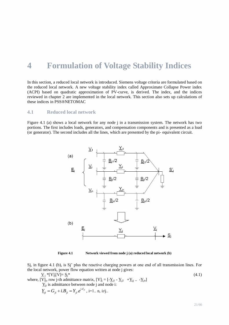
Figure 4.1 (a) shows a local network for any node j in a transmission system. The network has two

portions. The first includes loads, generators, and compensation components and is presented as a load (or generator). The second includes all the lines, which are presented by the pi- equivalent circuit.

Figure 4.1 Network viewed from node j (a) reduced local network (b)

Sj, in figure 4.1 (b), is Sj‟ plus the reactive charging powers at one end of all transmission lines. For the local network, power flow equation written at node j gives:

V j *[Y]j[V]= Sj* (4.1)

where, [Y]j, row j-th admittance matrix, [Y]j = [-Yj1 - Yj2 +Yjj .. -Yjn]

Yji is admittance between node j and node i: .

. . jii

ji ji ji jiY G i B Y e

, i=1.. n, i≠j..

22/66

Yjj is self admittance at node j:

Yjj=1,

n

ji

i i j

Y

=.

. jji

jjY e

[V], nodal voltages, [V]=

1

2

..

n

V

V

V

Expanding eq. (4.1), and letting1,

.n

ji i

i i j

j

jj

Y V

EY

gives:

* *.( ).j j j jj jV E V Y S (4.2)

Equation (4.2) is the load flow equation of 2 node system shown in figure 4.1 (b). The local network is reduced to an equivalent two node system, where Ej, and Yjj are the equivalent voltage, and the

equivalent admittance (self admittance) of the network seen from node j respectively.

Let ej= j

j

V

E, and divide both sides of equation (4.2) over

2

j jjE Y gives:

.2 . ji

j j jje e e S

, j j j (4.3)

where, .jj jj jjS P i Q , normalized nodal power

cos sin1. .

sin cos.

jj jj jj j

jj jj jj jjj j

P P

Q QY E

(4.4)

Separating (4.3) into real and imagine components:

2 .cosj j j jje e P (4.5)

.sinj j jje Q (4.6)

4.2 Formulation of voltage stability indices

4.2.1 Siemens specific formulation of stability criteria

Eliminate j from equations (4.5), and (4.6) one gets a quadratic equation of 2

je

2

2 2 2 21 2. .( ) 0j jj j jj jje P e P Q (4.7)

The condition for existing at least one solution different to 0 of equation (4.7) are:

1jj (4.8)

1 2. 0jjP (4.9)

where,

2 2 2

2 2

4. 4.

(1 2. )1 2.

jj jj jj

jj

jjjj

P Q S

PP

(4.10)

Under these conditions, je can be expressed as:

23/66

1 2.

. 1 12

jj

j jj

Pe

(4.11)

Divide equation (1.6) over -je and take absolute value gives:

jjjj eQ /sin (4.12)

At the voltage collapse point, we have 1jj , insert the value into equation (4.11) gives:

1 2..

2

jj

j

Pe

(4.13)

From equations (1.13) and (1.10) with 1jj gives:

2

jj jS e (4.14)

Magnitude of jjS is calculated from equation (4.4)

2.

j

jj

jj j

SS

Y E (4.15)

From (1.14), (1.15), with reminding that j

j

j

Ve

E then:

2

j

jj jL

j

SY Y

V (4.16)

Thus, at the voltage collapse point load admittance is equal to the self admittance of the network. The

condition is corresponding with the condition for maximum power transfer from the network to load at node j.

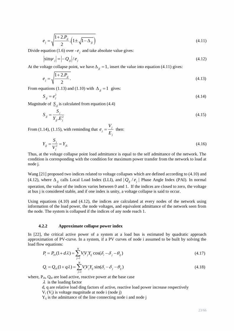
Wang [21] proposed two indices related to voltage collapses which are defined according to (4.10) and

(4.12), where jj calls Local Load Index (LLI), and | / |jj jQ e Phase Angle Index (PAI). In normal

operation, the value of the indices varies between 0 and 1. If the indices are closed to zero, the voltage at bus j is considered stable, and if one index is unity, a voltage collapse is said to occur.

Using equations (4.10) and (4.12), the indices are calculated at every nodes of the network using information of the load power, the node voltages, and equivalent admittance of the network seen from

the node. The system is collapsed if the indices of any node reach 1.

4.2.2 Approximate collapse power index

In [22], the critical active power of a system at a load bus is estimated by quadratic approach approximation of PV-curve. In a system, if a PV curves of node i assumed to be built by solving the

load flow equations:

0

1

(1 ) cos( )N

i i i j ij i j ij

j

P P d VV Y

(4.17)

0

1

(1 ) sin( )N

i i i j ij i j ij

j

Q Q q VV Y

(4.18)

where, Pi0, Qi0 are load active, reactive power at the base case

is the loading factor

d, q are relative load ding factors of active, reactive load power increase respectively

Vi (Vj) is voltage magnitude at node i (node j)

Yij is the admittance of the line connecting node i and node j

24/66

i ( j ) is phase angle of voltage phasor at node i (node j)

ij is phase angle of the admittance of the line connecting node i and node j

The quadratic approach assumes a second-order approximation for the plot of ( )iV f defined as:

2

i i i i i iaV bV c (4.19)

The first-order derivative /i idV d and the second-order derivative 2 2/i id V d are found as follows:

2 i i

i

da b

dV

(4.20)

1

2

i

i i

dV

d a b

(4.21)

23

22 ( )i i

i

d V dVa

d d (4.22)

Coefficients ai, bi, and ci are found by solving the equations as follows: 2 2

3

/

2( / )

ii

i

d V da

dV d

(4.23)

12

/i i i

i

b aVdV d

(4.24)

2

i i i i ic aV bV (4.25)

where, Vi is the voltage calculated from the load flow equations, and the first and second order

derivatives /i idV d and2 2/i id V d are calculated from the appendix 1

The critical voltage which corresponding to the maximum coefficient ,c i is obtained by taking (4.20)

equal to zero, which gives:

, / (2 )c i i iV b a (4.26)

The maximum coefficient ,c i is obtained by inserting Vc,i into (4.19):

2

, , ,c i i c i i c i iaV bV c (4.27)

Based on the approximation of the collapse active power, a new index, Approximate Collapse Power

Index (ACPI), is defined as:

, ,

1

1

i

c i c i

PACPI

P d

(4.28)

ACPI will vary from the range from 0 to 1. At low load levels, the index is close to 0. When the

system goes to critical point, ACPI reaches unity.

4.2.3 Applying of previous indices in the reduced local network

It shows that from a load bus, the system can be viewed as an equivalent voltage Ej connecting with the load bus through a self admittance Yjj. It is suitable to apply previous indices based on the reduced

local network defined in figure 4.1

▪ Line stability index: applying the same criteria to the reduced local network, formula (3.1)

becomes:

2

4 sin

([ sin( )]jj j

QLmn

Y E

(4.29)

25/66

where, Q is load reactive power

is the self admittance phase angle

is the angle difference between the equivalent voltage Ej and the load voltage Vj

Yjj is the self admittance magnitude of the local network viewed from the load bus

Ej is the equivalent voltage magnitude of the local network viewed from the load bus

▪ Voltage collapse proximity index: using the equivalent parameters of the reduced local network,

index VCPI from (3.2) is rewritten as:

1j

j

j

EVCPI

V (4.30)

where, Ej is the equivalent voltage phasor of the local network viewed from the load bus Vj is the load bus voltage phasor.

▪ Line power transfer stability index: to implement the index in the reduced local network, there are

two assumptions. Beside power factor of the load is assumed constant, the equivalent voltage

magnitude Ej is assumed not vary with the load voltage. Under these assumptions, PTSI can be

rewritten as follows:

2

2 [1 cos( )]L

jj j

SPTSI

Y E

(4.31)

where, SL is the load apparent power

is the phase angle of the load admittance

is the phase angle of the self admittance viewed from the load bus

Yjj is the self admittance of the local network viewed from the load bus

Ej is the equivalent voltage magnitude of the local network viewed from the load bus.

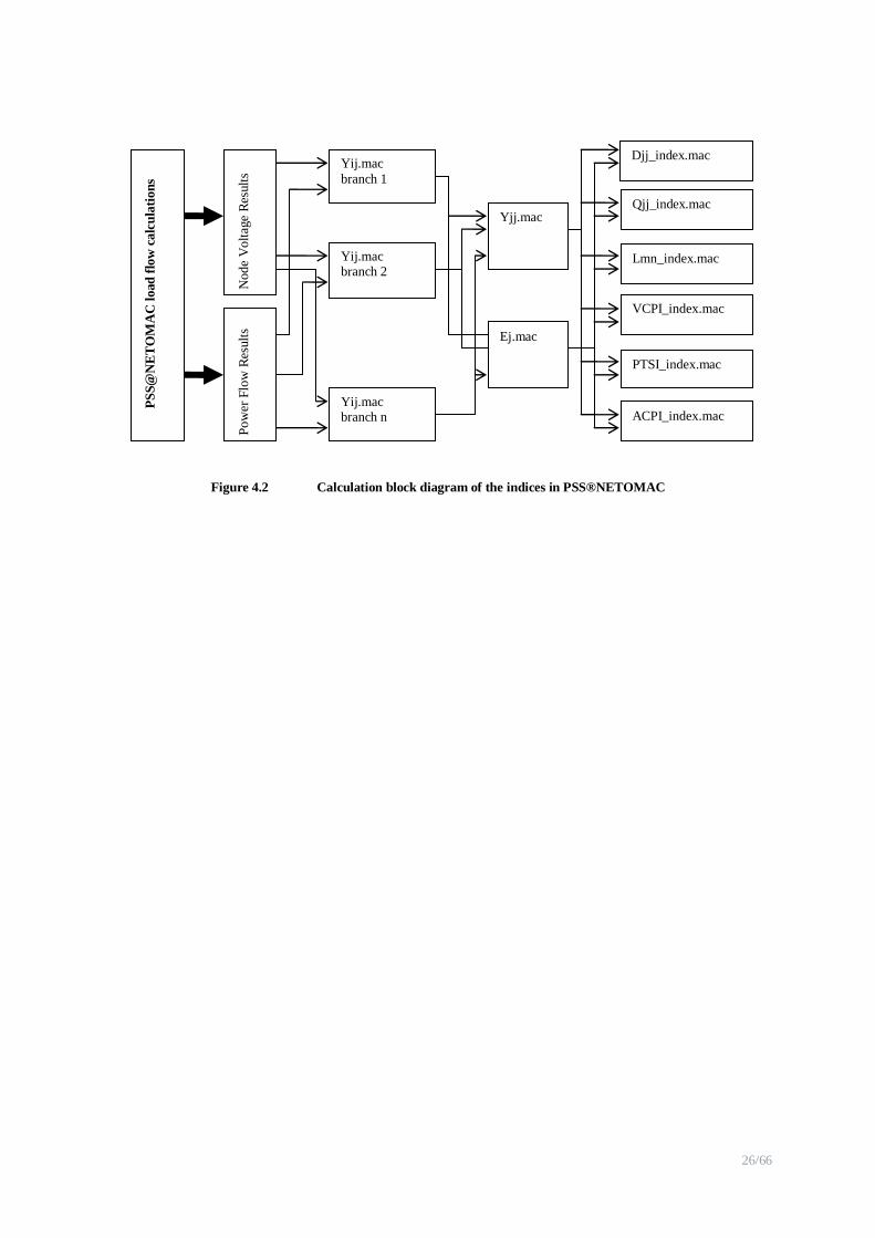
4.2.4 Calculating the indices in PSS®NETOMAC

All the indices are calculated based on the reduced local network. The calculations of the indices only base on the information of the load bus voltage and power, its surrounding bus voltage and the

admittance between the load bus and participating buses. The indices can be easy implemented in

PSS®NETOMAC based on several macros, some of which are presented in appendix A3. The

calculation algorithm of the indices is shown in figure 4.2, where:

▪ Yij.mac: this macro reads the voltage of two ends of a branch and current flow on the branch. The

output of this macro is the admittance of the branch.

▪ Yjj.mac: this macro evaluates the line admittance of participating line to calculate the self

admittance of the local network viewed from the load bus.

▪ Ej.mac: this macro evaluates the line admittance of participating line, self admittance at the load

bus and information of participating bus voltages. The output of this macro is the equivalent

voltage of the local network viewed from the load bus.

▪ Finally, each index can be calculated separately using the equivalent local network parameters.

26/66

Figure 4.2 Calculation block diagram of the indices in PSS®NETOMAC

PS

S@

NE

TO

MA

C l

oad

flo

w c

alc

ula

tion

s

Sta

bil

ity c

alcu

lati

on

Node

Volt

age

Res

ult

s

Pow

er F

low

Res

ult

s

Yij.mac

branch 1

Yij.mac branch 2

Yij.mac branch n

Yjj.mac

Ej.mac

Djj_index.mac

Qjj_index.mac

Lmn_index.mac

VCPI_index.mac

PTSI_index.mac

ACPI_index.mac

27/66

5 Simulation Results and Discussions

This section tests voltage stability indices through two test systems: 9 bus-3 generator test network and a larger test network including 414 buses, and 119 generators. In the smaller network, static analysis

and dynamic simulation are implemented. In the static analysis, PV curve of the system is built by

gradually increasing loads at a bus until the load flow program is diverged. Two cases are implemented, with and without considering reactive power limit of generators, to investigate the

affects of reactive power limits of generators in the load flow feasibility. For dynamic simulations, the

affects of AVR and OXL are examined. Line contingencies of the system are studied to show that the

indices are useful for line contingency ranking. For every test, the indices are investigated and compared regarding to sensitivities. It shows that all indices have coherent performances relating to

voltage stability. They are close 0 when the system is stable, and increase towards 1 when the system

is more critical. Two most sensitive indices, APCI and PTSI, are used to study the larger test system for different disturbances, load increasing and line disconnections. The calculation times of indices are

compared based on dynamic simulations of the larger test network.

5.1 9 bus system test

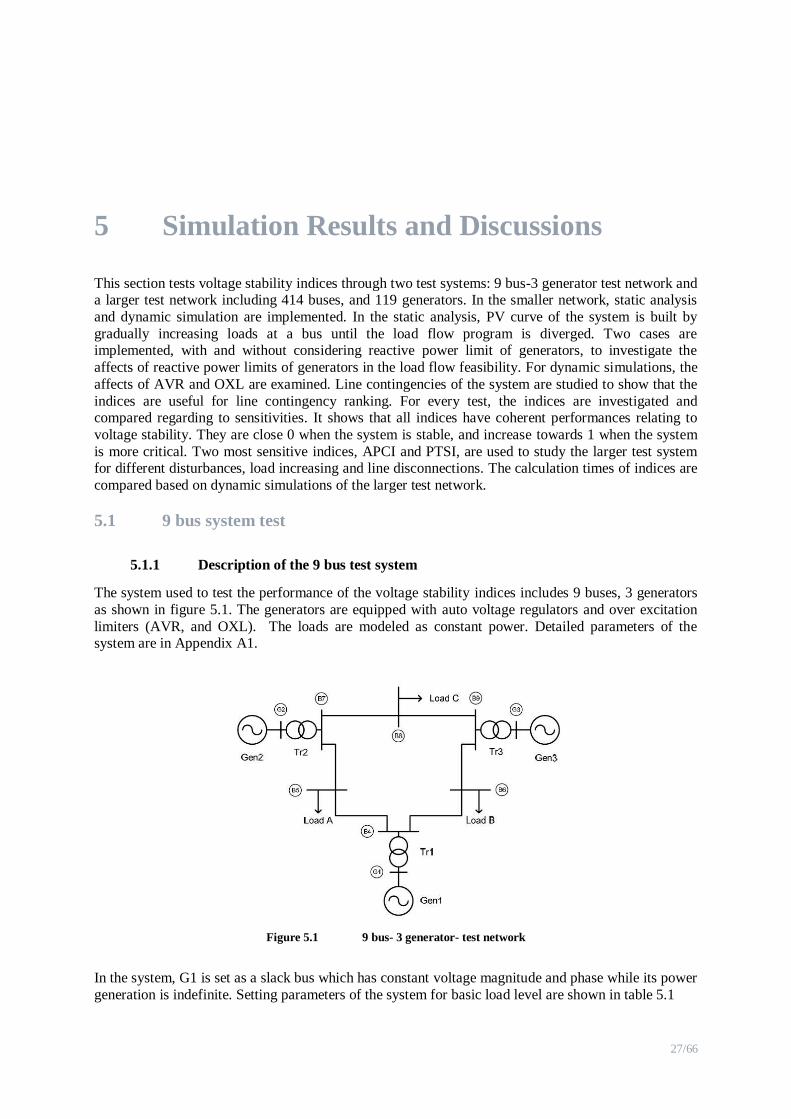
5.1.1 Description of the 9 bus test system

The system used to test the performance of the voltage stability indices includes 9 buses, 3 generators

as shown in figure 5.1. The generators are equipped with auto voltage regulators and over excitation

limiters (AVR, and OXL). The loads are modeled as constant power. Detailed parameters of the system are in Appendix A1.

Figure 5.1 9 bus- 3 generator- test network

In the system, G1 is set as a slack bus which has constant voltage magnitude and phase while its power

generation is indefinite. Setting parameters of the system for basic load level are shown in table 5.1

28/66

Bus Type V (p.u) Phase

(deg.)

P (MW) Q (MVar)

G1 Slack 1.00 0 x x

G2 PV 1.00 x 163.2 x

G3 PV 1.00 x 108.8 x

B5 PQ x x -100 -50

B6 PQ x x -100 -50

B8 PQ x x -100 -50

Table 5.1 9 bus test network setting at base load level

In table 5.1, positive powers imply the power injecting into the system (for generators), while negative

powers indicates the power consumed by the loads. All unknowns are marked as „x‟ is found after load

flow calculations.

5.1.2 Static analysis

In static approach, PV curves are built at every load bus by increasing load at bus 5 while the loads at

bus 6, 8 are kept constant. For each load level of load at bus 5, running power flow program to get the

corresponding voltages of the buses. All indices are also calculated. The increase of load is continued

until the load flow is diverged. There are two cases setting for the test. In the first case, reactive power

limits of generators are ignored while in the second including the reactive power limit of generators.

In this test, the maximum reactive power that load at bus 5 can consume in the first case is much

higher than that in the latter. This implies that reactive power of generators is a main contributor to the

loadability of the system. The loadability of the system is much smaller when considering the limit of

reactive power sources.

The results show that performances of indices are in agreement to each other and to the voltage

instability. At the base case, the indices are small, close 0, means that the system is stable. When the

loads are higher, the indices are higher. At load level where the power flow calculation diverges, the

indices close 1 indicates that the system is collapsed. Among all indices, index ACPI seem to be the

most sensitive one.

With static approach, the indices are good indicators for ranking the critical bus. Since load at bus 5 is

increased, the indices at the bus are increased and have highest values compared to those at bus 6, 8;

this load bus is the most critical one.

5.1.2.1 Case 1 without limitation of reactive power generators

In this case, maximum of reactive power of generators are not defined. It implies that the generators

are able to generate as much reactive power as the system required. During load flow calculation, voltage magnitudes of generator terminals are always constant. Table 5.2-5.4 shows the voltage of

buses and corresponding indices to increasing active power load at bus 5.

P5(MW) V5 (p.u.) D55 |Q55/e5| VCPI5 PTSI5 Lmn5 ACPI5

99,99 0,954 0,005 0,030 0,036 0,107 0,063 0,198

199,99 0,921 0,024 0,063 0,078 0,220 0,131 0,355

299,97 0,897 0,064 0,101 0,129 0,342 0,207 0,491

399,94 0,823 0,142 0,148 0,196 0,481 0,297 0,619

499,88 0,736 0,313 0,217 0,306 0,661 0,425 0,759

29/66

549,81 0,648 0,534 0,286 0,434 0,806 0,546 0,864

559,72 0,559 0,666 0,324 0,517 0,872 0,612 0,908

Table 5.2 Static analysis at bus 5 without considering reactive power limits of generators

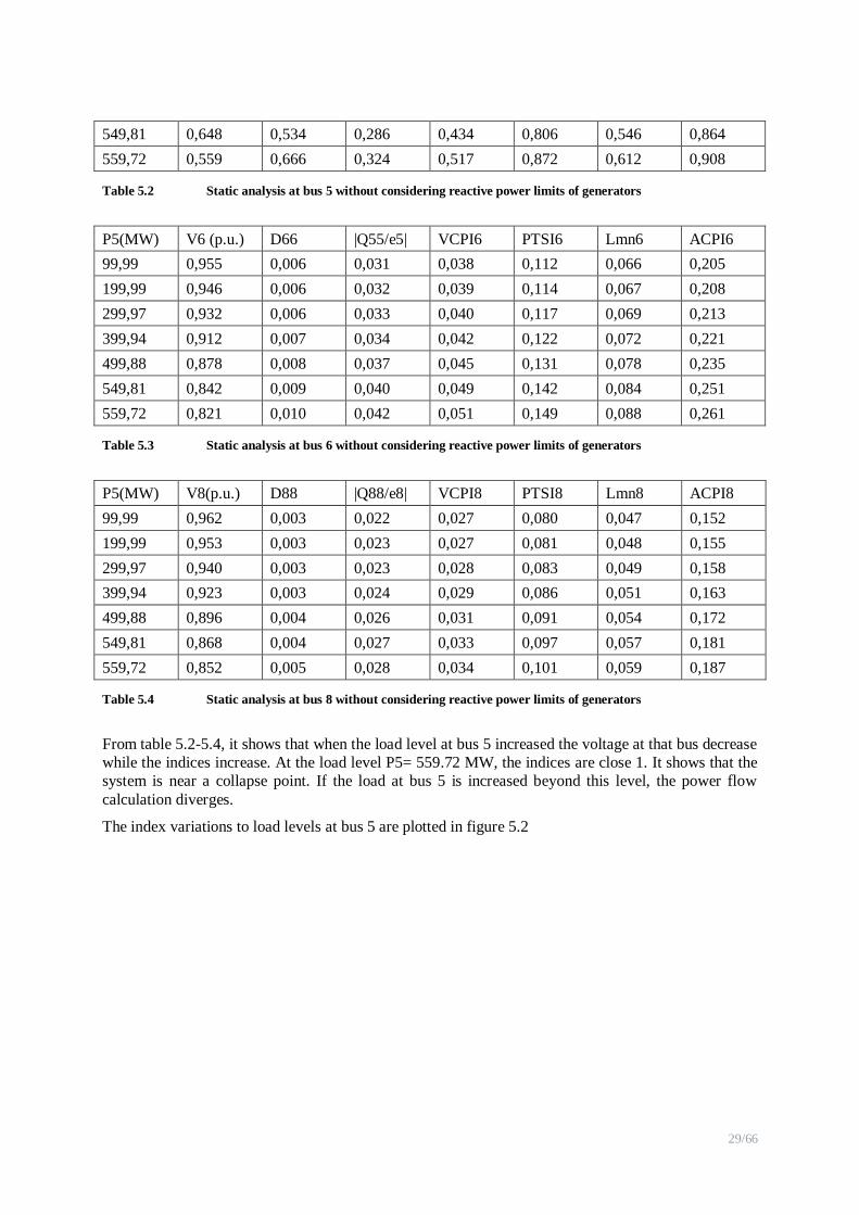
P5(MW) V6 (p.u.) D66 |Q55/e5| VCPI6 PTSI6 Lmn6 ACPI6

99,99 0,955 0,006 0,031 0,038 0,112 0,066 0,205

199,99 0,946 0,006 0,032 0,039 0,114 0,067 0,208

299,97 0,932 0,006 0,033 0,040 0,117 0,069 0,213

399,94 0,912 0,007 0,034 0,042 0,122 0,072 0,221

499,88 0,878 0,008 0,037 0,045 0,131 0,078 0,235

549,81 0,842 0,009 0,040 0,049 0,142 0,084 0,251

559,72 0,821 0,010 0,042 0,051 0,149 0,088 0,261

Table 5.3 Static analysis at bus 6 without considering reactive power limits of generators

P5(MW) V8(p.u.) D88 |Q88/e8| VCPI8 PTSI8 Lmn8 ACPI8

99,99 0,962 0,003 0,022 0,027 0,080 0,047 0,152

199,99 0,953 0,003 0,023 0,027 0,081 0,048 0,155

299,97 0,940 0,003 0,023 0,028 0,083 0,049 0,158

399,94 0,923 0,003 0,024 0,029 0,086 0,051 0,163

499,88 0,896 0,004 0,026 0,031 0,091 0,054 0,172

549,81 0,868 0,004 0,027 0,033 0,097 0,057 0,181

559,72 0,852 0,005 0,028 0,034 0,101 0,059 0,187

Table 5.4 Static analysis at bus 8 without considering reactive power limits of generators

From table 5.2-5.4, it shows that when the load level at bus 5 increased the voltage at that bus decrease

while the indices increase. At the load level P5= 559.72 MW, the indices are close 1. It shows that the

system is near a collapse point. If the load at bus 5 is increased beyond this level, the power flow

calculation diverges.

The index variations to load levels at bus 5 are plotted in figure 5.2

30/66

Figure 5.2 Static analysis at bus 5 without reactive power limits of generators

Figure 5.2 (a), (b), and (c) are the variations to load levels at bus 5 of voltage and indices at bus 5, 6,

and 8 respectively. At every bus, it shows that when the load level grows the voltage at that bus

decreases while the indices increase. The variation of voltage and indices at bus 5 grow sharply since

the system is stressed directly from this bus while at bus 6 and bus 8 the changes are slowly. At the

point close to the maximum power point, the indices at bus 5 are close unity. The figure shows that

index ACPI is the most sensitive and linear one because it has higher value and goes faster than other

indices when the load at bus 5 increases.

From figure 5.2 (a), it can be seen that index D55 are the smallest at lower load level at bus 5 (e.g.

P5=100-400 MW). However, it increases sharply, greater than |Q55/e5|, VCPI5, and Lmn5 when the

load level is higher.

From figure 5.2 (b), and (c), it shows that the voltages change slowly, and the indices are almost

unchanged when the load level at bus 5 grows. The reason is that the loads at these buses are constant

so the changes of indices depend almost on the drop of voltage at these bus and their surrounding

buses.

Figure 5.2 (d) shows more clearly the relation of voltage and indices with load levels at bus 5. It

presents the voltages and index ACPI at each bus. From the figure, at the base case, the voltages at

every bus are at high level, and the value of VCPI6 is highest, which implies that bus 6 is the most

critical one. At higher load level at bus 5, the voltages are smaller, and index VCPI5 is the highest. It

shows that bus 5 is the most critical bus in the system.

5.1.2.2 Case 2 including reactive power generator limitations

In load flow model, it is necessary to consider the ability of generators whether it is available to supply

reactive power demands of the system. To determine the range of reactive power limits of generators, capability curve of the generators can be used [13]. The capability curve of generator varies with the

excitation voltages. This causes impossible to calculate exactly the range of reactive power of

generators. However, in this study, the value can be estimated by assuming the excitation voltage is 1 (p.u.). Notice that the initial value of generator G2, and G3 are at its rating power, therefore the

maximum reactive power of these generators are determined directly through the rating power, and the

power factor of the generators. The maximum reactive power of G2, and G3 are shown in table 5.5

31/66

G2 G3

Rating (MVA) 192 128

Power factor 0.85 0.85

Active power (MW) 163,2 108,8

Maximum reactive power (MVar) 101,6 64,7

Table 5.5 Maximum reactive power of generators

With the setting of reactive power limit of generators above, power flow calculations are performed

the same as in previous case by increasing load at bus 5. The results of this test are shown in table 5.6-

5.8, and in figure 5.3

P(MW) V5 (p.u.) D55 |Q88/e8| VCPI5 PTSI5 Lmn5 ACPI5

99,99 0,954 0,005 0,030 0,036 0,107 0,063 0,198

199,99 0,920 0,024 0,063 0,078 0,221 0,131 0,356

299,97 0,817 0,085 0,116 0,149 0,387 0,235 0,535

350,04 0,718 0,183 0,167 0,225 0,534 0,333 0,662

359,98 0,681 0,233 0,188 0,257 0,588 0,372 0,705

365,10 0,647 0,284 0,207 0289 0637 0,407 0,741

Table 5.6 Static analysis at bus 5 considering reactive power limits of generators

P(MW) V6 (p.u.) D66 |Q88/e8| VCPI6 PTSI6 Lmn6 ACPI6

99,99 0,955 0,006 0,031 0,038 0,112 0,066 0,205

199,99 0,943 0,006 0,032 0,039 0,114 0,068 0,209

299,97 0,876 0,008 0,037 0,045 0,132 0,078 0,235

350,04 0,809 0,011 0,043 0,053 0,153 0,091 0,267

359,98 0,783 0,013 0,046 0,056 0,162 0,096 0,280

365,10 0,759 0,014 0,049 0,060 0,172 0,102 0,294

Table 5.7 Static analysis at bus 6 considering reactive power limits of generators

P(MW) V8 (p.u.) D88 |Q88/e8| VCPI8 PTSI8 Lmn8 ACPI8

99,99 0,962 0,003 0,022 0,027 0,080 0,047 0,152

199,99 0,950 0,003 0,023 0,027 0,082 0,048 0,155

299,97 0,863 0,004 0,028 0,033 0,098 0,058 0,183

350,04 0,777 0,007 0,034 0,041 0,120 0,071 0,218

359,98 0,744 0,008 0,037 0,045 0,131 0,077 0,233

365,10 0,714 0,009 0,040 0,049 0,141 0,084 0,249

Table 5.8 Static analysis at bus 8 considering reactive power limits of generators

32/66

Figure 5.3 Static analysis considering reactive power limits of generators

Figure 5.3 (a), (b), and (c) are the relations of voltage and indices corresponding to load level at bus 5

for bus 5, 6, and 8 respectively. The performance of voltages and indices at each node are the same as

in previous case. When the load level at bus 5 is higher, the voltages at every bus are lower and the

indices are higher. However, the difference is that the maximum loading power at load 5 is only

365.10 MW, much smaller than that in the previous case. The difference of voltages, and index

performances to load level at bus 5 at two cases is recognized more clearly in figure 5.4.

Figure 5.4 Static analysis of bus 5 at two cases

33/66

Figure 5.4 shows the relations between voltage V5 and index ACPI5 in two cases. From this figure, it

shows that when the system is at low load level, the voltage and the index in two cases are equal.

When the load is higher, the voltage and index change steeper for the case considering reactive power

limit. This is due to the reason that the generators have supplied all its reactive power. From modeling

as PV nodes which have constant terminal voltages, generators are changed into PQ node, its voltage

is decreased when the load increases. This shows that considering reactive power limit of generators

will reduce the ability of the system regarding to voltage stability.

5.1.2.3 Remarks of static tests

Thorough the static analysis, some remarks are pointed out as following:

▪ All indices are in agreement with each other and coherent with voltage stability of the system

▪ The indices at each bus are sensitive with the change of load at that bus only, e.g. ACPI5 changes

sharply when load at bus 5 increases while ACPI6, and ACPI 8 are almost unchanged. Therefore,

the indices are useful to evaluate the critical bus in a power system.

▪ Index Djj is not sensitive at low load level but it gets higher sensitivity than |Qjj/ej|, VCPIj, Lmnj,

when the load is close to critical point.

▪ ACPI and PTSI seem to be the most sensitive indices to the load change.

5.1.3 Dynamic analysis

In the dynamic simulation of voltage collapse for the 9 bus test system, two operating conditions have been considered to investigate the effect of the AVR and OXL. The contingency considered for the

operating conditions is by increasing the static load at bus 5 at a rate of 0.05 (p.u./sec). The power at

bus 5 is defined as follows:

0 (1 0.05* )tP P t (MW) (5.1)

0 (1 0.05* )tQ Q t (MVar) (5.2)

During simulation, the indices are calculated and their performances are then compared. The system is

said collapse if any of the indices reaches unity.

5.1.3.1 Effects of AVR and OXL

Case1: The first operating condition considers only static loads connected at buses 5, 6 and 8. The

voltage collapse indicators, Djj, PTSI, VCPI, Lmn, and VCPI at the load buses 5, 6 and 8 are plotted

against time as shown in Figure 5.5

34/66

Figure 5.5 Dynamic simulations without considering AVR and OXL

From the figure, it can be seen that the indices increase with time as loads are increased and the indicators at bus 5 give the highest values compared to the indicators at bus 6 and 8. The figure also

shows that system voltage collapse occurs at time t = 18 sec

Case2: The second operating point incorporates both AVR and OXL in the generators. The result is shown in figure 5.6.

Figure 5.6 Dynamic simulations with affects of AVR and OXL

35/66

For this case, voltage collapse occurs at 23.5 sec which shows that voltage collapse occurs later than

for the case without AVR and OXL. This is because of the effect of the AVR and OXL which

maintain a constant generator voltage by increasing the field current while load is increased.

5.1.3.2 Line contingencies

This section tests the performance of indices according to line contingencies using dynamic simulations. The system is equipped with AVR and OXL. After each line contingency, the system

variables change, the indices are recorded at the time when the system goes to steady state. The results

of the test are shown in tables 5.9-5.11 and figure 5.7.

Line

Disconnection

V5 (p.u.) D55 |Q55/e5| VCPI5 PTSI5 Lmn5 ACPI5

No 0.954 0,005 0,030 0,036 0,107 0,063 0,198

LB7-B8 0,953 0,005 0,030 0,037 0,108 0,063 0,199

LB8-B9 0,946 0,005 0,031 0,037 0,109 0,064 0,201

LB9-B6 0,937 0,006 0,031 0,038 0,111 0,066 0,204

LB6-B4 0,957 0,005 0,030 0,036 0,107 0,063 0,197

LB4-B5 0,912 0,027 0,067 0,083 0,233 0,139 0,371

LB5-B7 0,908 0,023 0,062 0,077 0,27 0,129 0,352

Table 5.9 Contingency analysis at bus 5

Line

Disconnection

V6 (p.u.) D66 |Q66/e6| VCPI6 PTSI6 Lmn6 ACPI6

No 0,955 0,005 0,031 0,038 0,112 0,066 0,205

LB7-B8 0,933 0,006 0,033 0,040 0,117 0,069 0,213

LB8-B9 0,962 0,006 0,031 0,037 0,110 0,065 0,202

LB9-B6 0,906 0,028 0,068 0,084 0,235 0,141 0,375

LB6-B4 0,912 0,027 0,067 0,083 0,232 0,139 0,371

LB4-B5 0,958 0,006 0,031 0,038 0,111 0,066 0,204

LB5-B7 0,933 0,006 0,033 0,040 0,117 0,069 0,213

Table 5.10 Contingency analysis at bus 6

Line

Disconnection

V8 (p.u.) D88 |Q88/e8| VCPI8 PTSI8 Lmn8 ACPI8

No 0,962 0,003 0,022 0,027 0,080 0,047 0,152

LB7-B8 0,904 0,024 0,063 0,078 0,219 0,131 0,354

LB8-B9 0,935 0,009 0,038 0,046 0,135 0,080 0,240

LB9-B6 0,964 0,003 0,022 0,027 0,079 0,047 0,152

LB6-B4 0,950 0,003 0,023 0,027 0,082 0,048 0,156

LB4-B5 0,947 0,003 0,023 0,028 0,082 0,048 0,156

LB5-B7 0,960 0,003 0,022 0,027 0,080 0,047 0,153

Table 5.11 Contingency analysis at bus 8

36/66

Figure 5.7 Line contingencies and index performances

In the tables 5.9-5.11, and figure 5.7, „No‟ is corresponding to the normal operating condition. Figures

5.7 (a)-(c) illustrate the variations to different line contingencies of the indices at bus 5, 6, and 8

respectively. From the figures, it shows that from the normal operating condition the indices jump to

higher values when a line is disconnected. The indices have significant value at bus where has direct

connection with the disconnected line. For example, the indices at bus 5 are higher than those at bus 6,

8 as the disconnected lines are „LB4-LB5‟, „LB5-LB7‟. Similarly, the indices at bus 6, 8 are

significantly high as these are „LB9-B6‟, „LB6-B4‟, and „LB7-B8‟, „LB8-B9‟, respectively. The

reason is that when a line is switch off, the self admittance of the reduced local network at node j,

which directly connected to the disconnected line are decreased. This causes the loadability of the

reduced local network lessen and hence the indices jump up.

The sensitivity of the indices to the line contingencies are also shown clearly in the figure. It shows

that Djj has the smallest sensitivity while ACPI has the highest. Relying on the index, line contingency

ranking can be obtained by set ACPIj as the maximum value of ACPI5, ACPI6, and ACPI8, then

sorting the line contingencies according to ACPIj. Table 5.12 shows the rank of line contingencies

based on the evaluation of the index.

Line

Disconnection

Vj (p.u.) Djj |Qjj/ej| VCPIj PTSIj Lmnj ACPIj Rank

LB4-B5 0,91 0,028 0,068 0,085 0,236 0,141 0,376 1

LB9-B6 0,905 0,028 0,068 0,084 0,236 0,141 0,375 2

LB6-B4 0,912 0,027 0,067 0,083 0,233 0,139 0,372 3

LB5-B7 0,906 0,024 0,063 0,078 0,221 0,131 0,356 4

LB7-B8 0,903 0,024 0,063 0,078 0,22 0,131 0,355 5

LB8-B9 0,934 0,009 0,038 0,046 0,135 0,08 0,241 6

No 0,962 0,003 0,022 0,027 0,08 0,047 0,152 7

Table 5.12 Line contingency ranking with index ACPI

37/66

In table 5.12, Vj, and Djj to Lmnj are voltage, and indices which are corresponding to ACPIj. From

the table, it points that „LB4-B5‟ outage is the most severe line contingency in the system.

5.1.3.3 Remarks of the dynamic tests

From the dynamic analysis, some remarks are pointed out as followings:

▪ Effects of AVR and OXL are to strengthen the system regarding to voltage instability by increasing

excitation voltage of generators so that maintaining the voltage at generators terminals.

▪ Performances of the indices in dynamic simulations are coincided with them in the static analysis.

The indices are small, close to 0 at lower load levels and they move towards 1 when the load

increases to the loadability limit.

▪ PTSI and ACPI seem to be the most sensitive and linear indices compared to others. A comparison

of these indices regarding to sensitivity is shown in table 5.13, where more + sign indicates better

sensitive

Indices Djj |Qjj/ej| VCPI PTSI Lmn ACPI

Sensitivity + + + +++ ++ ++++

Table 5.13 Sensitivity comparison of the indices

5.2 Larger network test

Previous parts have tested the performances of indices based on the 9 bus test system. The results show that two indices ACPI and PTSI are sensitive and linear to voltage instability of the system. In

this section, these indices are applied in a larger test network to evaluate the feasibility of the indices

in a more practical network.

5.2.1 Description of the larger test network

The test network is built based on a practical power system including 119 Generators, 527 transmission lines, 261 transformers and 414 nodes. An overview of the network is illustrated in

figure A.2 in the appendix.

The power system consists of three parts: the north, center, and the south. In normal operating

condition, the total generating power is 18.67 GW out of 26.36 GW. There are 4 high voltage levels

500 kV (80 nodes and 180 transmission lines), 230 kV (80 nodes and 180 lines), 115 kV (199 nodes and 314 lines) and 69 kV (4 nodes and 2 lines). The center and southern areas are connected through

long tie-lines near 800 km. High load increase in the southern areas, or line outages in the tie-lines

could cause severe problem to the system. These contingencies will be investigated in the test. The test network is modeled in PSS®NETOMAC with the features as followings:

▪ Synchronous machines are modeled based on Park model.

▪ There are 24 generators are equipped speed governor of either IEEEG1 type (Figure A.6 a) or

HYGOV type (Figure A.6b). They are both IEEE standard governors and defined in PSS®

NETOMAC database.

▪ There are three types of AVR being used by all of 119 generators. They are IEEET1 type (Figure

A.5a), EXAC4 type (Figure A.5b), SCRX type (Figure A.5c).

5.2.2 Load increasing

As mention earlier, load increasing in the south could make a severe problem to the network. In this

case, bus SRT___00 is chosen for studying. This bus is an important bus in the southern area which

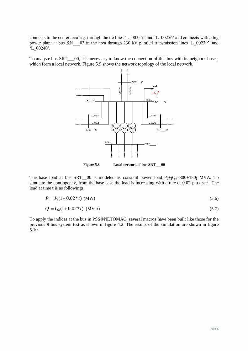
38/66

connects to the center area e.g. through the tie lines „L_00255‟, and „L_00256‟ and connects with a big

power plant at bus KN___03 in the area through 230 kV parallel transmission lines „L_00239‟, and

„L_00240‟.

To analyze bus SRT___00, it is necessary to know the connection of this bus with its neighbor buses,

which form a local network. Figure 5.9 shows the network topology of the local network.

Figure 5.8 Local network of bus SRT___00

The base load at bus SRT__00 is modeled as constant power load P0+jQ0=300+150j MVA. To

simulate the contingency, from the base case the load is increasing with a rate of 0.02 p.u./ sec. The

load at time t is as followings:

0 (1 0.02* )tP P t (MW) (5.6)

0 (1 0.02* )tQ Q t (MVar) (5.7)

To apply the indices at the bus in PSS®NETOMAC, several macros have been built like those for the

previous 9 bus system test as shown in figure 4.2. The results of the simulation are shown in figure

5.10.

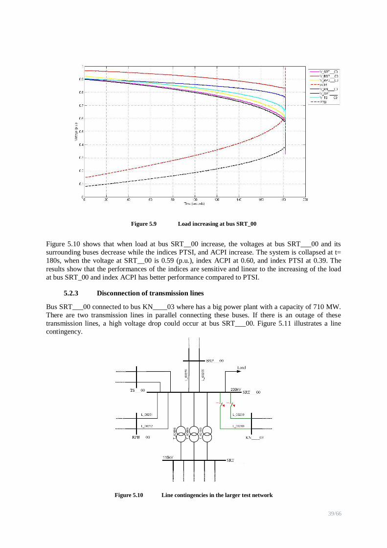
39/66

Figure 5.9 Load increasing at bus SRT_00

Figure 5.10 shows that when load at bus SRT__00 increase, the voltages at bus SRT___00 and its

surrounding buses decrease while the indices PTSI, and ACPI increase. The system is collapsed at t=

180s, when the voltage at SRT__00 is 0.59 (p.u.), index ACPI at 0.60, and index PTSI at 0.39. The

results show that the performances of the indices are sensitive and linear to the increasing of the load

at bus SRT_00 and index ACPI has better performance compared to PTSI.

5.2.3 Disconnection of transmission lines

Bus SRT___00 connected to bus KN____03 where has a big power plant with a capacity of 710 MW.

There are two transmission lines in parallel connecting these buses. If there is an outage of these

transmission lines, a high voltage drop could occur at bus SRT___00. Figure 5.11 illustrates a line contingency.

Figure 5.10 Line contingencies in the larger test network

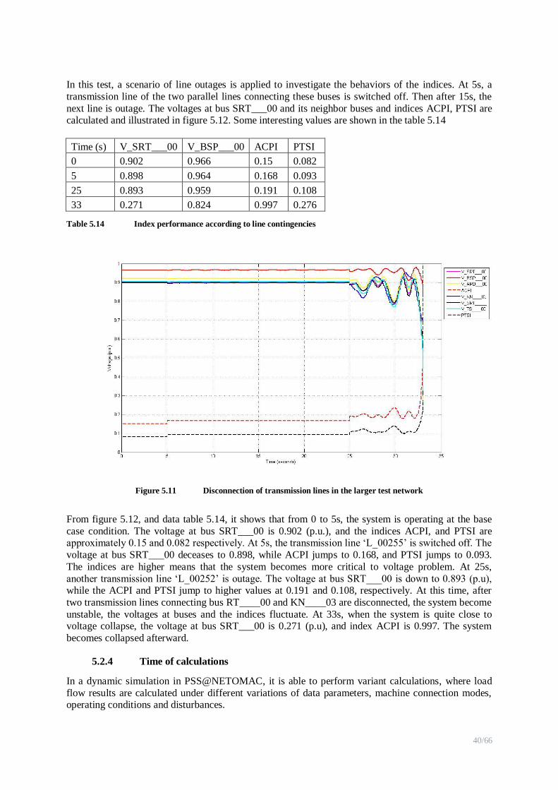
40/66

In this test, a scenario of line outages is applied to investigate the behaviors of the indices. At 5s, a

transmission line of the two parallel lines connecting these buses is switched off. Then after 15s, the

next line is outage. The voltages at bus SRT___00 and its neighbor buses and indices ACPI, PTSI are calculated and illustrated in figure 5.12. Some interesting values are shown in the table 5.14

Time (s) V_SRT___00 V_BSP___00 ACPI PTSI

0 0.902 0.966 0.15 0.082

5 0.898 0.964 0.168 0.093

25 0.893 0.959 0.191 0.108

33 0.271 0.824 0.997 0.276

Table 5.14 Index performance according to line contingencies

Figure 5.11 Disconnection of transmission lines in the larger test network

From figure 5.12, and data table 5.14, it shows that from 0 to 5s, the system is operating at the base

case condition. The voltage at bus SRT___00 is 0.902 (p.u.), and the indices ACPI, and PTSI are approximately 0.15 and 0.082 respectively. At 5s, the transmission line „L_00255‟ is switched off. The

voltage at bus SRT___00 deceases to 0.898, while ACPI jumps to 0.168, and PTSI jumps to 0.093.

The indices are higher means that the system becomes more critical to voltage problem. At 25s,

another transmission line „L_00252‟ is outage. The voltage at bus SRT___00 is down to 0.893 (p.u), while the ACPI and PTSI jump to higher values at 0.191 and 0.108, respectively. At this time, after

two transmission lines connecting bus RT____00 and KN____03 are disconnected, the system become

unstable, the voltages at buses and the indices fluctuate. At 33s, when the system is quite close to voltage collapse, the voltage at bus SRT___00 is 0.271 (p.u), and index ACPI is 0.997. The system

becomes collapsed afterward.

5.2.4 Time of calculations

In a dynamic simulation in PSS@NETOMAC, it is able to perform variant calculations, where load

flow results are calculated under different variations of data parameters, machine connection modes, operating conditions and disturbances.

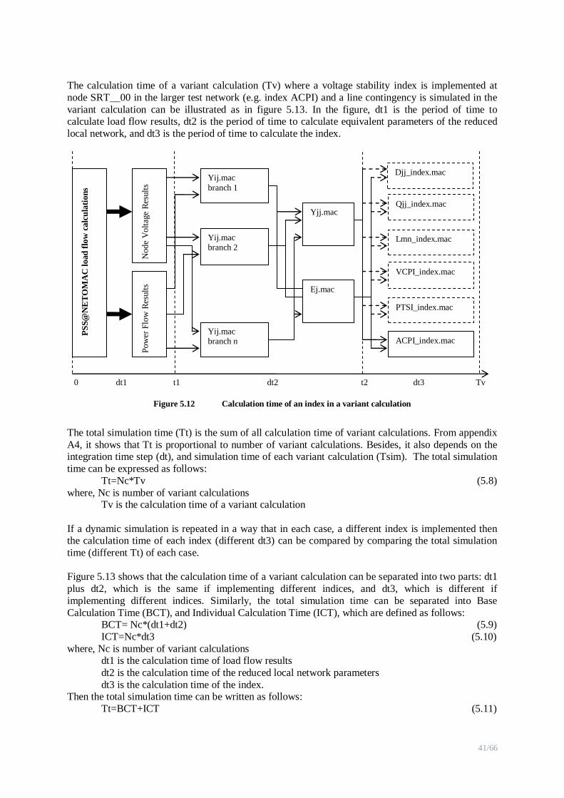
41/66

The calculation time of a variant calculation (Tv) where a voltage stability index is implemented at

node SRT__00 in the larger test network (e.g. index ACPI) and a line contingency is simulated in the

variant calculation can be illustrated as in figure 5.13. In the figure, dt1 is the period of time to calculate load flow results, dt2 is the period of time to calculate equivalent parameters of the reduced

local network, and dt3 is the period of time to calculate the index.

Figure 5.12 Calculation time of an index in a variant calculation

The total simulation time (Tt) is the sum of all calculation time of variant calculations. From appendix

A4, it shows that Tt is proportional to number of variant calculations. Besides, it also depends on the integration time step (dt), and simulation time of each variant calculation (Tsim). The total simulation

time can be expressed as follows:

Tt=Nc*Tv (5.8)

where, Nc is number of variant calculations Tv is the calculation time of a variant calculation

If a dynamic simulation is repeated in a way that in each case, a different index is implemented then the calculation time of each index (different dt3) can be compared by comparing the total simulation

time (different Tt) of each case.

Figure 5.13 shows that the calculation time of a variant calculation can be separated into two parts: dt1

plus dt2, which is the same if implementing different indices, and dt3, which is different if

implementing different indices. Similarly, the total simulation time can be separated into Base

Calculation Time (BCT), and Individual Calculation Time (ICT), which are defined as follows: BCT= Nc*(dt1+dt2) (5.9)

ICT=Nc*dt3 (5.10)

where, Nc is number of variant calculations dt1 is the calculation time of load flow results

dt2 is the calculation time of the reduced local network parameters

dt3 is the calculation time of the index. Then the total simulation time can be written as follows:

Tt=BCT+ICT (5.11)

PS

S@

NE

TO

MA

C l

oad

flo

w c

alc

ula

tion

s

Sta

bil

ity c

alcu

lati

on

Node

Volt

age

Res

ult

s

Pow

er F

low

Res

ult

s

Yij.mac

branch 1

Yij.mac branch 2

Yij.mac branch n

Yjj.mac

Ej.mac

Djj_index.mac

Qjj_index.mac

Lmn_index.mac

VCPI_index.mac

PTSI_index.mac

ACPI_index.mac

dt2

dt3

dt1

0

t1

t2

Tv

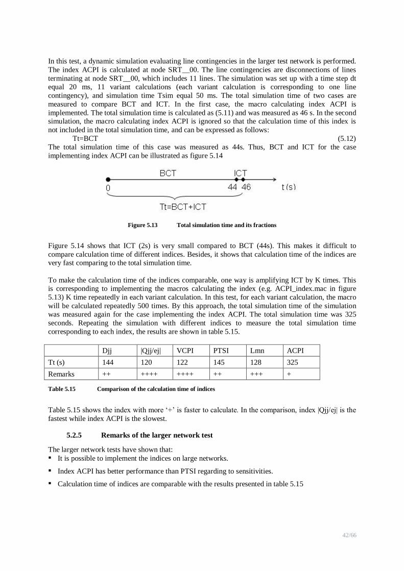
42/66

In this test, a dynamic simulation evaluating line contingencies in the larger test network is performed.

The index ACPI is calculated at node SRT__00. The line contingencies are disconnections of lines

terminating at node SRT__00, which includes 11 lines. The simulation was set up with a time step dt equal 20 ms, 11 variant calculations (each variant calculation is corresponding to one line

contingency), and simulation time Tsim equal 50 ms. The total simulation time of two cases are

measured to compare BCT and ICT. In the first case, the macro calculating index ACPI is

implemented. The total simulation time is calculated as (5.11) and was measured as 46 s. In the second simulation, the macro calculating index ACPI is ignored so that the calculation time of this index is

not included in the total simulation time, and can be expressed as follows:

Tt=BCT (5.12) The total simulation time of this case was measured as 44s. Thus, BCT and ICT for the case

implementing index ACPI can be illustrated as figure 5.14

Figure 5.13 Total simulation time and its fractions

Figure 5.14 shows that ICT (2s) is very small compared to BCT (44s). This makes it difficult to

compare calculation time of different indices. Besides, it shows that calculation time of the indices are very fast comparing to the total simulation time.

To make the calculation time of the indices comparable, one way is amplifying ICT by K times. This is corresponding to implementing the macros calculating the index (e.g. ACPI_index.mac in figure

5.13) K time repeatedly in each variant calculation. In this test, for each variant calculation, the macro

will be calculated repeatedly 500 times. By this approach, the total simulation time of the simulation was measured again for the case implementing the index ACPI. The total simulation time was 325

seconds. Repeating the simulation with different indices to measure the total simulation time

corresponding to each index, the results are shown in table 5.15.

Djj |Qjj/ej| VCPI PTSI Lmn ACPI

Tt (s) 144 120 122 145 128 325

Remarks ++ ++++ ++++ ++ +++ +

Table 5.15 Comparison of the calculation time of indices

Table 5.15 shows the index with more „+‟ is faster to calculate. In the comparison, index |Qjj/ej| is the

fastest while index ACPI is the slowest.

5.2.5 Remarks of the larger network test

The larger network tests have shown that:

▪ It is possible to implement the indices on large networks.

▪ Index ACPI has better performance than PTSI regarding to sensitivities.

▪ Calculation time of indices are comparable with the results presented in table 5.15

43/66

6 Conclusion

This thesis evaluates the existing Siemens‟ voltage stability criteria Djj, |Qjj|/ej by comparing its performance with some well-known voltage stability indices including Lmn, VCPI, PTSI, and a new

proposed index based on quadratic approximation of PV curves, ACPI. All indices are applied in the

reduced local network. The calculation algorithm of these indices in simulation tool PSS®NETOMAC is presented.

The performances of these indices are verified through both steady state and dynamic analysis. They

are tested in the 9 bus- 3 generator system, and the more practical, larger network including 414 buses, and 119 generators. It shows that their performances are coherent to each other regarding to voltage

stability of the system. All indices fall between 0 and 1. When the system is stable, these indices are

closed 0. When the system is more critical, the indices move towards closed to 1, but with different levels of convergence to 1.

The performances of the indices regarding to sensitivity, and calculation time can be summarized as in table 6.1, where more „+‟ sign indicates better performance.

Djj |Qjj/ej| VCPI PTSI Lmn ACPI

Sensitivity + + + +++ ++ ++++

Calculation

time ++ ++++ ++++ ++ +++ +

Table 6.1 Comparison of the indices

Table 6.1 shows that Siemens criteria Djj, |Qjj/ej| are less sensitive compared to other indices,

however, they have advantages of fast calculation time, especially, index |Qjj/ej|. Index ACPI is the most sensitive one, however, costs more computational time. Since all the indices are very fast to be

calculated, index ACPI is highly recommended to be implemented in a voltage assessment module in

the power system simulator PSS®NETOMAC

In this thesis, test systems are equipped with AVR and OXL. The loads are modeled as constant power

loads. Some indices such as PTSI, ACPI are defined under assumptions that the equivalent voltage of

the local network is constant with the variation of load power.

For more intensive study, the system should be modeled more detailed, e.g. with existences of on-load

tap changer transformers, and dynamic loads. For more accuracy in calculation of indices PTSI, and ACPI, it is capable to use Thevenin equivalent voltage and impedance viewed from a load bus instead

of the local network parameters. Therefore, it is maybe useful to track Thevenin equivalent parameters

in the simulation tool PSS®NETOMAC

44/66

References

[1] W. Bialek: Cambridge Working Papers in Economics CWPE 0407, 2004

[2] T.V Cutsem: “Voltage stability of electric power system”, Springer, 1998

[3] G.K. Morison: “Voltage stability using static and dynamic approach”, in: IEEE Transaction on

Power Systems, Vol. 8, No. 3, August 1993, p. 88-100

[4] J.C. Chow: “On the evaluation of voltage collapse criteria”, in IEE Transaction on Power

Systems, Vol. 5, No. 2, May 1990, p. 612-620

[5] P.A. Lof: “Voltage stability indices for stressed power systems”, in IEEE Transaction on Power

Systems, Vol. 8, No. 1, February 1993, p. 326-335

[6] B. Gao: “Voltage stability evaluation using modal analysis”, in Transactions on Power Systems,

Vol. 7, No. 4, November 1992, p. 1529-1542

[7] B. Lee: “Invariant subspace parametric sensitivity (ISPS) of structure-preserving power system

models”, IEEE Transaction on Power System, Vol.11, No.2, May 1996, p. 845-850

[8] P. Kessel: “Estimating the voltage stability of a power system”, in IEEE Transaction on Power

Delivery, Vol. PWRD-1, No. 3, July 1986, p. 346-354

[9] M. Moghavemi: “Real-time contingency evaluation and ranking technique”, in IEE Procedure

on Generation, Transmission and Distribution, Vol. 145, No. 5, September 1998, p. 517-524

[10] V. Balamourougan: “Technique for online prediction of voltage collapse”, in IEE Procedure on

Generation, Transmission and Distribution, Vol.151, No. 4, July 2004, p. 453-460

[11] M.H. Haque: “On-line monitoring of maximum permissible loading of a power system within

voltage stability limits”, in IEE Procedure on Generation, Transmission and Distribution, Vol.

150, No. 1, January 2003, p. 107-112

[12] P. Kundur: “Definition and classification of power system stability”, in IEEE Transaction on

Power Systems, Vol.19, No. 2, May 20004, p. 1387-1401

[13] P. Kundur: “Power system stability and control”, McGraw-Hill, Inc, Palo Alto, California, 1994

[14] O. Ruhle: “PSS®NETOMAC application guilde”, Siemens AG, PTD PTI SE, 2003

[15] C.A. Canizares: “Basic theoretical concept, Chapter 5 Voltage stability indices”, in IEEE Power

Engineering Society, August 2004

[16] N. Flatabo: “Voltage stability condition in a power transmission system calculated by sensitivity

methods”, in IEEE Transaction on Power Systems, Vol. 5, No. 4, November 1990, p.1286-1295

[17] F. Gubina: “Voltage collapse proximity index determination using voltage phasor approach”, in

IEEE Transaction on Power Systems, Vol. 10, No. 2, p. 788-794

[18] M. Nizam: “Estimating the voltage stability of a power system”, in IEEE Transaction on Power

Delivery, Vol. PWRD-1, No. 3, July1986, p. 346-354

[19] T. An: “Research on illed-condition equations in tracking Thevenin equivalent parameters with

local measurement‟‟, International Conference on Power System Technology, 2006

45/66

[20] K. Vu: “Use of local measurements to estimate voltage stability margin‟‟, in IEEE Transaction

on Power System, Vol. 14, No. 3, August 1999, p. 1029-1235

[21] Z. Wang: “Master thesis: Investigation of voltage stability criteria to be used in DAS system‟‟,

RWTH Aachen University, 2009

[22] A. Pama: “A new approach for estimating voltage collapse point based on quadratic

approximation of PV-curves‟‟, in Electric Power System Research 79, 2009, p. 653-659

[23] “IEEE Recommended Practice for Excitation System Models for Power System Stability

Studies‟‟, IEEE Power Engineering Society, New York, April 2006.

46/66

Appendix

Appendix 1 Calculate the first-order and second- order derivative /i idV d and2 2/i id V d 47

Appendix 2 9 bus- 3 generator test system parameters ....................................................... 48

Appendix 3 Larger test network......................................................................................... 51

Appendix 4 Variations of total simulation time (Tt) to integration time step (dt) and number

of contingencies (Nc) ..................................................................................... 57

Appendix 5 Some macros used in the larger test network ................................................... 58

Appendix 6 Simulation results in PSS®NETOMAC .......................................................... 62

47/66

Appendix 1 Calculate the first-order and second- order derivative /i idV d and2 2/i id V d

Figure A.1 The reduced local network

Figure A1 illustrates a reduced local network viewed from a load bus. Power flow equations written at

the node are as follows: 2

0(1 ) sin( ) sin( )P P d YEV YV (A1.1)

2

0(1 ) cos( ) cos( )Q P q YEV YV (A1.2)

Where P, Q, and V are the powers, and voltage magnitude at the load bus

E ,Y are the equivalent voltage and self admittance of the local network viewed from the

load bus; 90

Assuming that the equivalent voltage E is constant, taking the first order derivative of (A1.1) and

(A1.2) to gives:

0 cos( ) [ sin( ) 2 sin ]dP d dV

P d YEV YE YVd d d

(A1.3)

0 sin( ) [ cos( ) 2 cos ]dQ d dV

Q q YEV YE YVd d d

(A1.4)

Solving equations (A1.3), (A1.4) for the first order derivatives /d d , and /dV d gives:

)cos2(

]]sin2)sin([]cos2)cos([ 00

VEYEV

qQVEdPVE

d

d

(A1.5)

0 0sin( ) cos( )

( 2 cos )

dP qQdV

d Y E V

(A1.6)

The second derivative of V to is calculated from partial derivatives as follows: 2

2( ) ( )

d V dV d dV dV

d d d V d d

(A1.7)

Taking derivative both sides of equation (A1.6) to give:

0 0 0 0

2

[cos( ) sin( ) ] 2 (cos sin )( )

( 2 cos )

E dP y qQ V dP qQdV

d Y E V

(A1.8)

Similarly, ( )dV

V d

is obtained by taking derivative both sides of equation (A1.6) to V:

0 0

2

2cos [sin( ) cos( ) ]( )

( 2 cos )

dP y qQdV

V d Y E V

(A1.9)

Finally, the second derivative of V to is calculated by inserting (A1.5) (A1.6), and (A1.8), (A1.9)

into (A1.7)

P+jQ

V Y E

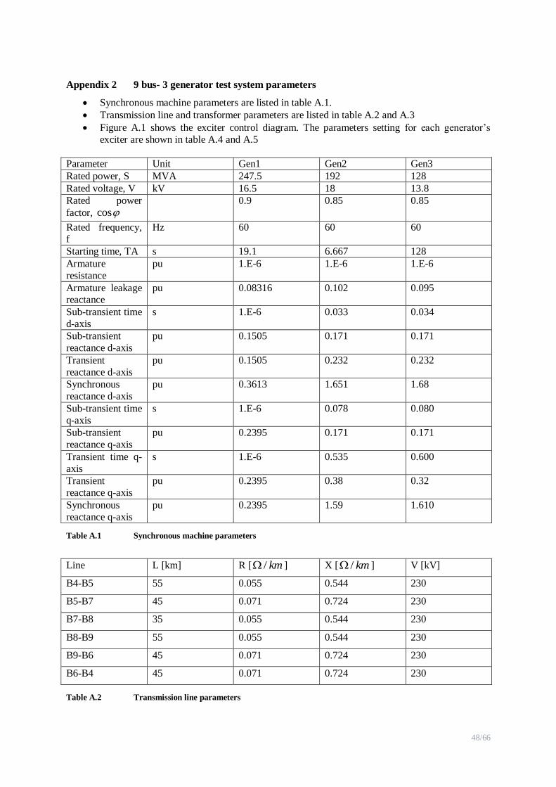
48/66

Appendix 2 9 bus- 3 generator test system parameters

Synchronous machine parameters are listed in table A.1.

Transmission line and transformer parameters are listed in table A.2 and A.3

Figure A.1 shows the exciter control diagram. The parameters setting for each generator‟s

exciter are shown in table A.4 and A.5

Parameter Unit Gen1 Gen2 Gen3

Rated power, S MVA 247.5 192 128

Rated voltage, V kV 16.5 18 13.8

Rated power

factor, cos

0.9 0.85 0.85

Rated frequency, f

Hz 60 60 60

Starting time, TA s 19.1 6.667 128

Armature

resistance

pu 1.E-6 1.E-6 1.E-6

Armature leakage reactance

pu 0.08316 0.102 0.095

Sub-transient time

d-axis

s 1.E-6 0.033 0.034

Sub-transient

reactance d-axis

pu 0.1505 0.171 0.171

Transient

reactance d-axis

pu 0.1505 0.232 0.232

Synchronous

reactance d-axis

pu 0.3613 1.651 1.68

Sub-transient time

q-axis

s 1.E-6 0.078 0.080

Sub-transient

reactance q-axis

pu 0.2395 0.171 0.171

Transient time q-

axis

s 1.E-6 0.535 0.600

Transient

reactance q-axis

pu 0.2395 0.38 0.32

Synchronous

reactance q-axis

pu 0.2395 1.59 1.610

Table A.1 Synchronous machine parameters

Line L [km] R [ / km ] X [ / km ] V [kV]

B4-B5 55 0.055 0.544 230

B5-B7 45 0.071 0.724 230

B7-B8 35 0.055 0.544 230

B8-B9 55 0.055 0.544 230

B9-B6 45 0.071 0.724 230

B6-B4 45 0.071 0.724 230

Table A.2 Transmission line parameters

49/66

Parameter Unit T1 T2 T3

Rated power MVA 247.5 192 128

Connection Yy Yy Yy

Rated high

voltage side

kV 230 230 230

Rated low voltage

side

kV 16.5 18 13.8

Short circuit

voltage

% 12 8 8

Table A.3 Transformer parameters

Figure A.2 Excitation system type AC2A- [23]

Parameter Gen1 Gen2 Gen3 Comment

XDU 0.3613 1.651 1.68 Unsaturated Xd [pu] of the generator

XL 0.08316 0.102 0.095 Armature leakage reactance Xl [pu] of the

generator

Table A.4 Parameter setting of exciter type IEEE CA2A (a)

Parameter Setting value Comment

XDU 2.19 Unsaturated Xd [pu] of the generator

XL 0.156 Armature leakage reactance Xl [pu] of the generator

TR 0.02 Measuring time constant TR [s]

VAMAX1 20.93 AVR-limit VAmax1 [non-reciprocal pu of EFD]

VAMAX2 28.43 AVR-limit VAmax2 [non-reciprocal pu of EFD]

VAMIN1 0 AVR-limit VAmin1 [non-reciprocal pu of EFD]

VAMIN2 -28.43 AVR-limit VAmin2 [non-reciprocal pu of EFD]

VRMAX 70.31 CR-limit VRmax [non-reciprocal pu of EFD]

VRMIN1 -70.31 CR-limit VRmin1 [non-reciprocal pu of EFD]

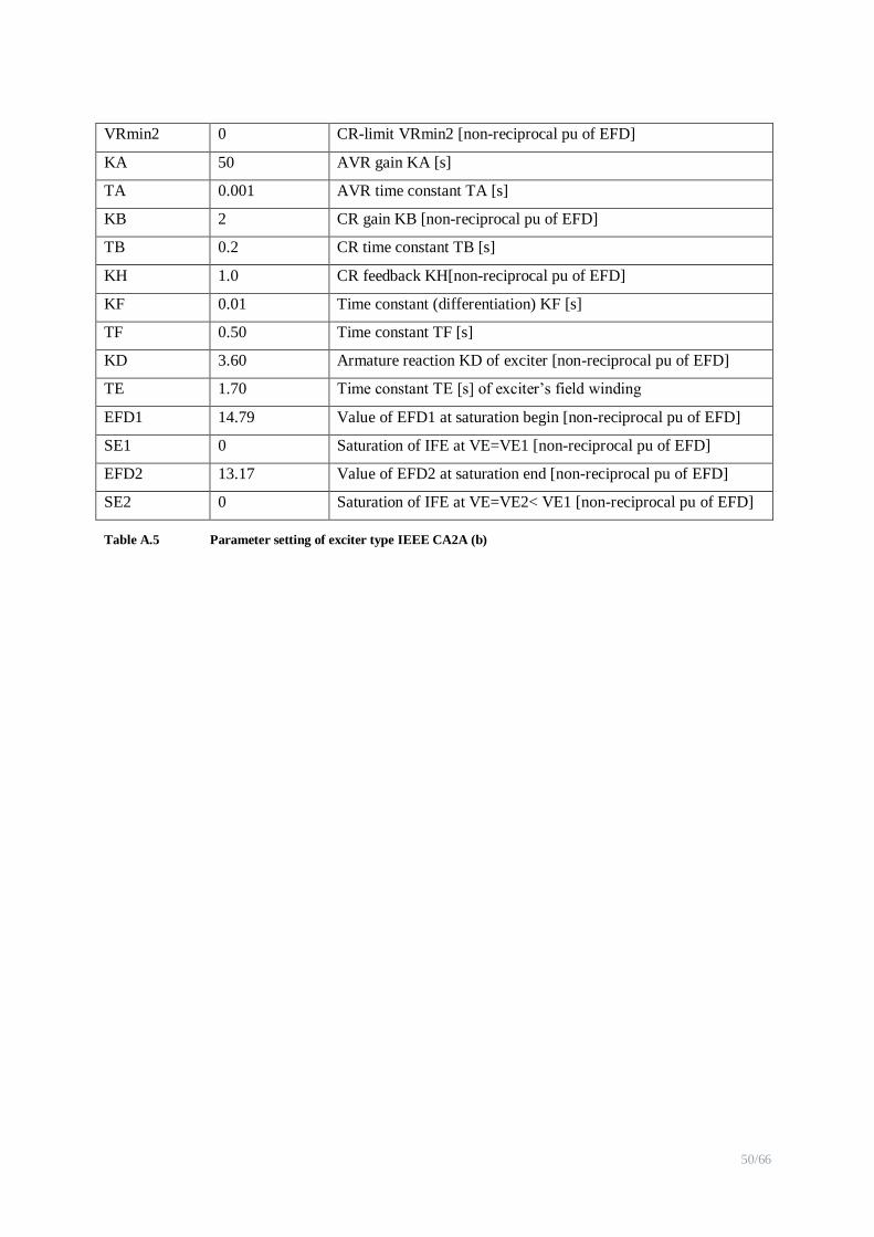
50/66

VRmin2 0 CR-limit VRmin2 [non-reciprocal pu of EFD]

KA 50 AVR gain KA [s]

TA 0.001 AVR time constant TA [s]

KB 2 CR gain KB [non-reciprocal pu of EFD]

TB 0.2 CR time constant TB [s]

KH 1.0 CR feedback KH[non-reciprocal pu of EFD]

KF 0.01 Time constant (differentiation) KF [s]

TF 0.50 Time constant TF [s]

KD 3.60 Armature reaction KD of exciter [non-reciprocal pu of EFD]

TE 1.70 Time constant TE [s] of exciter‟s field winding

EFD1 14.79 Value of EFD1 at saturation begin [non-reciprocal pu of EFD]

SE1 0 Saturation of IFE at VE=VE1 [non-reciprocal pu of EFD]

EFD2 13.17 Value of EFD2 at saturation end [non-reciprocal pu of EFD]

SE2 0 Saturation of IFE at VE=VE2< VE1 [non-reciprocal pu of EFD]

Table A.5 Parameter setting of exciter type IEEE CA2A (b)

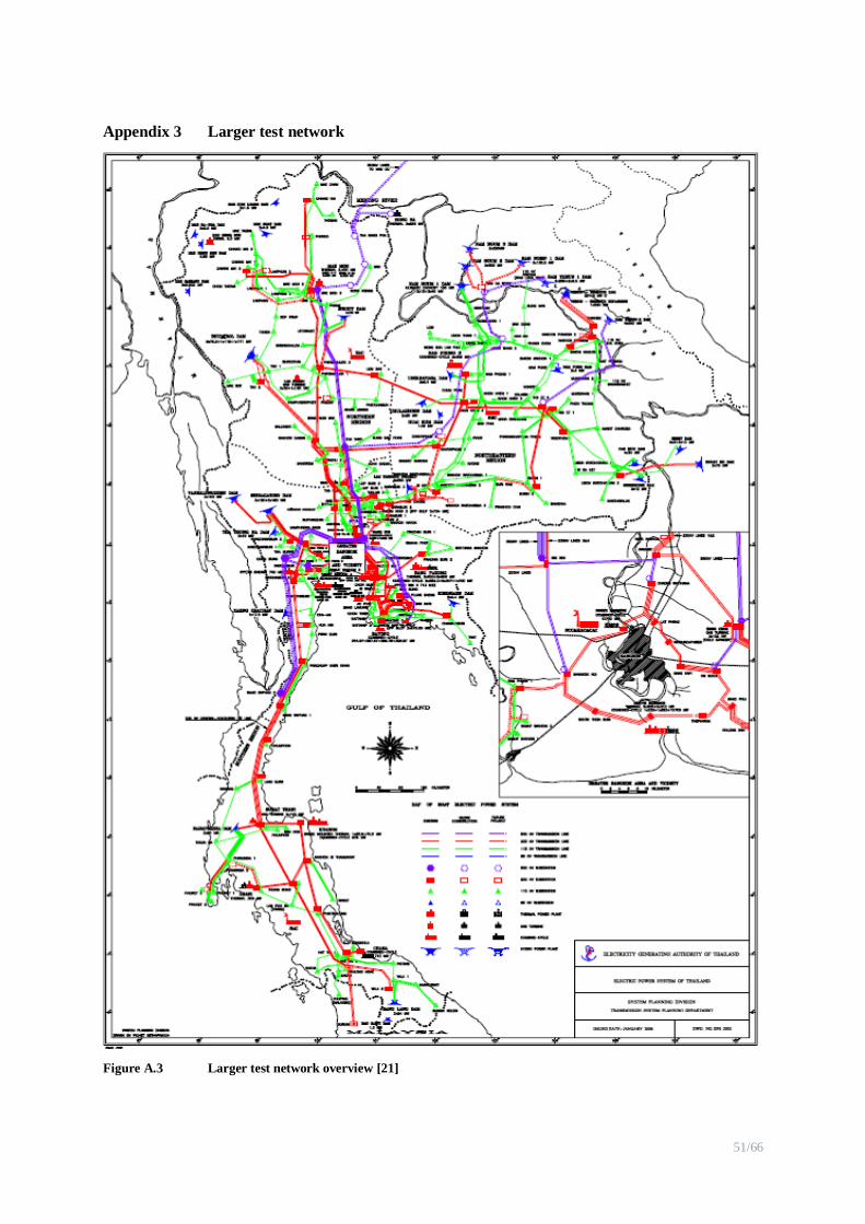
51/66

Appendix 3 Larger test network

Figure A.3 Larger test network overview [21]

52/66

Figure A.4 Contingency locations [21]

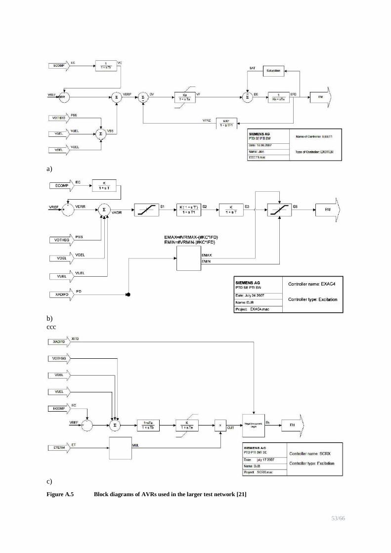
53/66

a)

b)

ccc

c)

Figure A.5 Block diagrams of AVRs used in the larger test network [21]

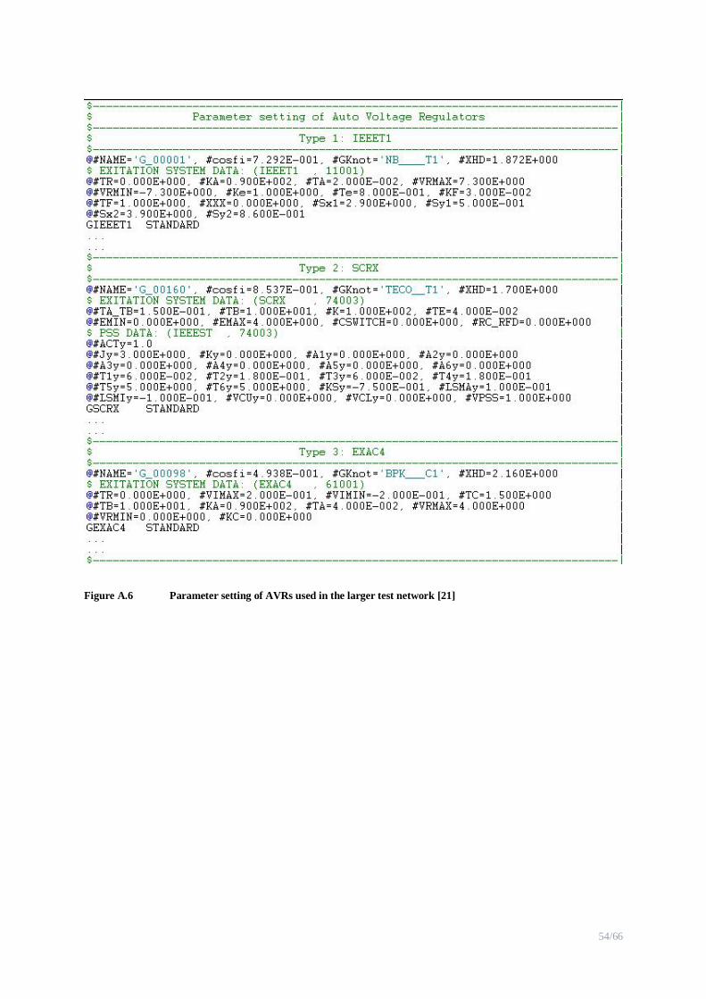
54/66

Figure A.6 Parameter setting of AVRs used in the larger test network [21]

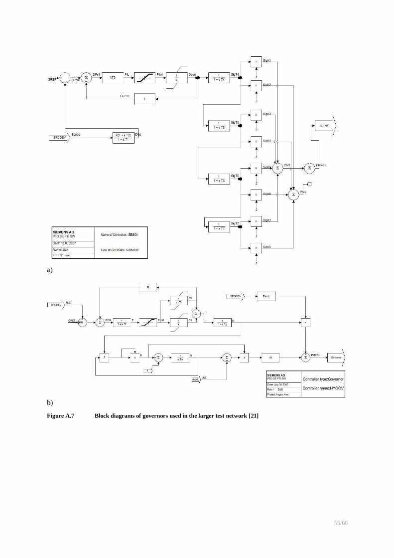
55/66

a)

b)

Figure A.7 Block diagrams of governors used in the larger test network [21]

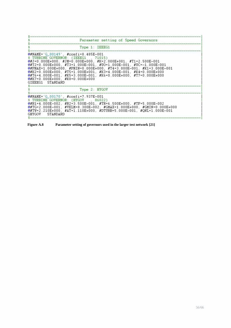
56/66

Figure A.8 Parameter setting of governors used in the larger test network [21]

57/66

Appendix 4 Variations of total simulation time (Tt) to integration time step (dt) and number

of contingencies (Nc)

To show the relation between total calculation time (Tt) to integration time step (dt), 60 variants of branch contingencies are applied in the larger test network where index ACPI is calculated at node

SRT___00. The simulation time of each variant calculation Tsim is 50s. The total calculation time is

counted from starting the simulation until the last results are achieved. For each dt, different Tt are obtained as shown in figure A.9

Figure A.9 Variation of the total simulation time to integration time step

From figure A.9, it shows that when the integration time step decreases, total calculation time

increases.

The total calculation time also depend on the number of contingencies analyzed, or number of variant

calculations. To show the relation between the total simulation time and the number of contingencies

(Nc), integration time step is selected as 20 ms, and simulation time of each variant is Tsim equal 50s. For the simulation where index ACPI is calculated, with each Nc, Tt is counted and illustrated in

figure A.10

Figure A.10 Variation of the total simulation time to the number of contingencies

From figure 5.10, it shows that Tc is proportional to Nc

58/66

Appendix 5 Some macros used in the larger test network

Figure A.11 Macro calculating branch admittance Yij.mac

59/66

Figure A.12 Macro calculating the self admittance Yjj.mac (cont)

60/66

Figure A.13 Macro calculating the self admittance Yjj.mac

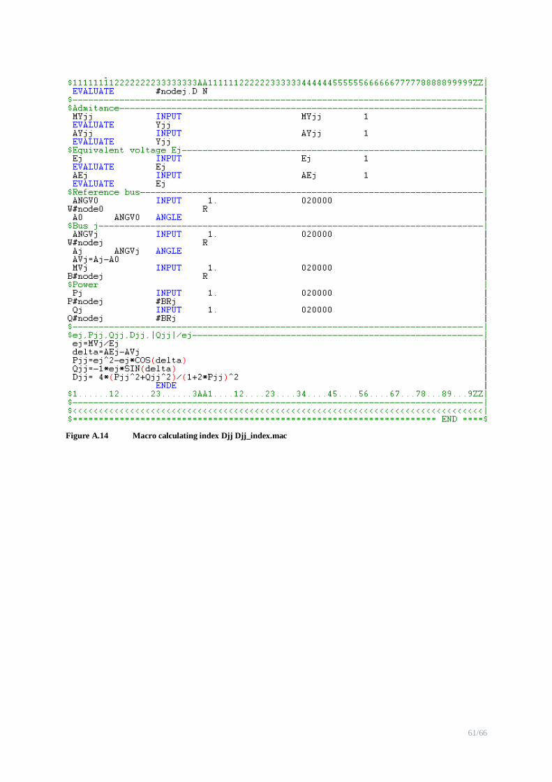
61/66

Figure A.14 Macro calculating index Djj Djj_index.mac

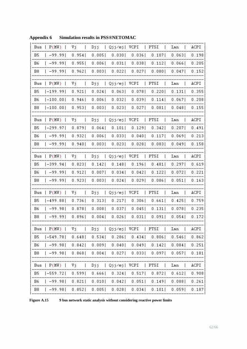
62/66

Appendix 6 Simulation results in PSS®NETOMAC

Figure A.15 9 bus network static analysis without considering reactive power limits

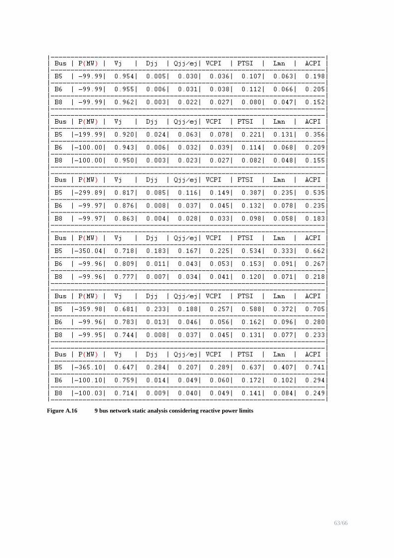
63/66

Figure A.16 9 bus network static analysis considering reactive power limits

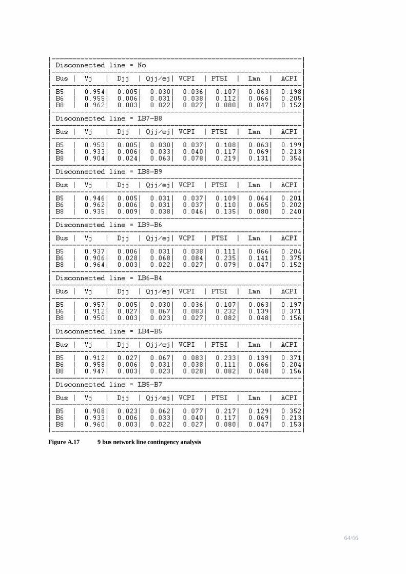
64/66

Figure A.17 9 bus network line contingency analysis

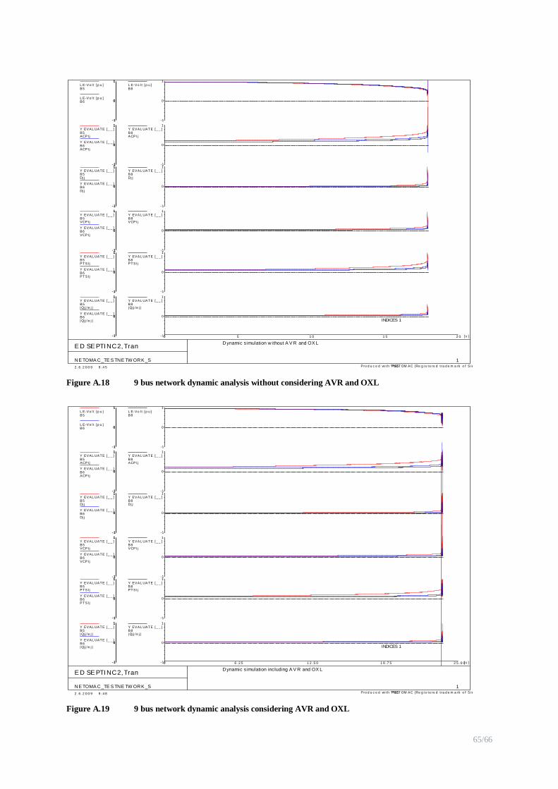
65/66

E D SE PTI NC2, Tran

Pro d u c e d wi th PSSTMNET OM AC (Re g i s te re d t ra d e m a rk o f Si e m e n s AG)

NE TOMA C_TE S TNE TW ORK _S

Dynamic simulation w ithout A V R and OX L

2 .6 .2 0 0 9 9 :4 5

1

INDICES 1

0 5 1 0 1 5 2 0 [s ]

-1

0

1L E-Vo l t [p u ]B8

-1

0

1Y EVAL UAT E [_ _ ]B8ACPI j

-1

0

1Y EVAL UAT E [_ _ ]B8Dj j

-1

0

1Y EVAL UAT E [_ _ ]B8VCPI j

-1

0

1Y EVAL UAT E [_ _ ]B8PT SI j

-1

0

1Y EVAL UAT E [_ _ ]B8| Qj j /e j |

-1

0

1L E-Vo l t [p u ]B5

-1

0

1Y EVAL UAT E [_ _ ]B5ACPI j

-1

0

1Y EVAL UAT E [_ _ ]B5Dj j

-1

0

1Y EVAL UAT E [_ _ ]B5VCPI j

-1

0

1Y EVAL UAT E [_ _ ]B5PT SI j

-1

0

1Y EVAL UAT E [_ _ ]B5| Qj j /e j |

-1

0

1

L E-Vo l t [p u ]B6

-1

0

1

Y EVAL UAT E [_ _ ]B6ACPI j

-1

0

1

Y EVAL UAT E [_ _ ]B6Dj j

-1

0

1

Y EVAL UAT E [_ _ ]B6VCPI j

-1

0

1

Y EVAL UAT E [_ _ ]B6PT SI j

-1

0

1

Y EVAL UAT E [_ _ ]B6| Qj j /e j |

Figure A.18 9 bus network dynamic analysis without considering AVR and OXL

E D SE PTI NC2, Tran

Pro d u c e d wi th PSSTMNET OM AC (Re g i s te re d t ra d e m a rk o f Si e m e n s AG)

NE TOMA C_TE S TNE TW ORK _S

Dynamic simulation including A V R and OX L

2 .6 .2 0 0 9 9 :4 8

1

INDICES 1

0 6 .2 5 1 2 .5 0 1 8 .7 5 2 5 .0 0[s ]

-1

0

1L E-Vo l t [p u ]B8

-1

0

1Y EVAL UAT E [_ _ ]B8ACPI j

-1

0

1Y EVAL UAT E [_ _ ]B8Dj j

-1

0

1Y EVAL UAT E [_ _ ]B8VCPI j

-1

0

1Y EVAL UAT E [_ _ ]B8PT SI j

-1

0

1Y EVAL UAT E [_ _ ]B8| Qj j /e j |

-1

0

1L E-Vo l t [p u ]B5

-1

0

1Y EVAL UAT E [_ _ ]B5ACPI j

-1

0

1Y EVAL UAT E [_ _ ]B5Dj j

-1

0

1Y EVAL UAT E [_ _ ]B5VCPI j

-1

0

1Y EVAL UAT E [_ _ ]B5PT SI j

-1

0

1Y EVAL UAT E [_ _ ]B5| Qj j /e j |

-1

0

1

L E-Vo l t [p u ]B6

-1

0

1

Y EVAL UAT E [_ _ ]B6ACPI j

-1

0

1

Y EVAL UAT E [_ _ ]B6Dj j

-1

0

1

Y EVAL UAT E [_ _ ]B6VCPI j

-1

0

1

Y EVAL UAT E [_ _ ]B6PT SI j

-1

0

1

Y EVAL UAT E [_ _ ]B6| Qj j /e j |

Figure A.19 9 bus network dynamic analysis considering AVR and OXL

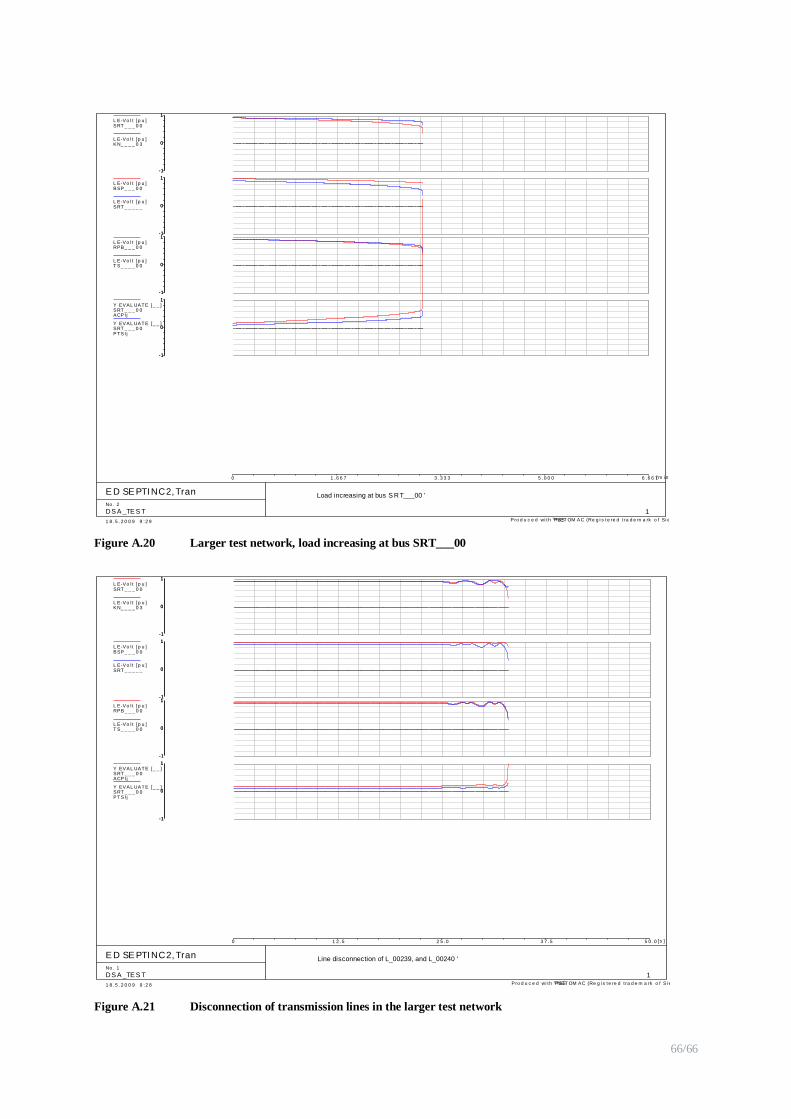
66/66

E D SE PTI NC2, Tran

Pro d u c e d wi th PSSTMNET OM AC (Re g i s te re d t ra d e m a rk o f Si e m e n s AG)

DS A _TE S T

Load increasing at bus S RT___00 '

1 8 .5 .2 0 0 9 9 :2 9

No . 2

1

0 1 .6 6 7 3 .3 3 3 5 .0 0 0 6 .6 6 7[m i n ]

-1

0

1L E-Vo l t [p u ]SRT _ _ _ 0 0

-1

0

1L E-Vo l t [p u ]BSP_ _ _ 0 0

-1

0

1L E-Vo l t [p u ]RPB_ _ _ 0 0

-1

0

1Y EVAL UAT E [_ _ ]SRT _ _ _ 0 0ACPI j

-1

0

1

L E-Vo l t [p u ]KN_ _ _ _ 0 3

-1

0

1

L E-Vo l t [p u ]SRT _ _ _ _ _

-1

0

1

L E-Vo l t [p u ]T S_ _ _ _ 0 0

-1

0

1

Y EVAL UAT E [_ _ ]SRT _ _ _ 0 0PT SI j

Figure A.20 Larger test network, load increasing at bus SRT___00

E D SE PTI NC2, Tran

Pro d u c e d wi th PSSTMNET OM AC (Re g i s te re d t ra d e m a rk o f Si e m e n s AG)

DS A _TE S T

Line disconnection of L_00239, and L_00240 '

1 8 .5 .2 0 0 9 9 :2 8

No . 1

1

0 1 2 .5 2 5 .0 3 7 .5 5 0 .0 [s ]

-1

0

1L E-Vo l t [p u ]SRT _ _ _ 0 0

-1

0

1L E-Vo l t [p u ]BSP_ _ _ 0 0

-1

0

1L E-Vo l t [p u ]RPB_ _ _ 0 0

-1

0

1Y EVAL UAT E [_ _ ]SRT _ _ _ 0 0ACPI j

-1

0

1

L E-Vo l t [p u ]KN_ _ _ _ 0 3

-1

0

1

L E-Vo l t [p u ]SRT _ _ _ _ _

-1

0

1

L E-Vo l t [p u ]T S_ _ _ _ 0 0

-1

0

1

Y EVAL UAT E [_ _ ]SRT _ _ _ 0 0PT SI j

Figure A.21 Disconnection of transmission lines in the larger test network