Catchment Modelling Strategies for Faecal Indicator Organisms:

Options Review and Recommendations

Project Code

WW0220

Workpakage 1; Milestone 2

Interim Report on Literature Review Listing Sources Accessed

January 2011

Project Team

David Oliver* (Principal Author of this Report),John Crowther**, Phil Haygarth***, Louise Heathwaite***,

David Kay**, Trevor Page***

* Stirling University; ** Aberystwyth University; *** Lancaster University

Correspondence to:-David Kay

dave@crehkay.demon.co.uk01570 423565 (Tel and Fax)

Page 1 of 37

GLOSSARY

Black-box model: A model which does not explicitly represent the actual processes in converting the model input into a model output.

Calibration: The fitting of model predictions with measured data through the changing of model input parameters relating to some accepted criteria.

Continuous model: The application of a model to continuous data (e.g. long term) as opposed to discrete data (e.g. storm event)

Deterministic: A deterministic model is one of knowable outcome: having an outcome that can be predicted because all of its causes are either known or the same as those of a previous event.

Empirical model: A model developed on empirical observations of the system under study

Export coefficient model: A ‘black-box’ modelling approach whereby, for a given climatic regime, a particular land use class is determined to export characteristic quantities of a contaminant over a defined time period.

Fully-distributed: The attributes of the catchment being modelled are distributed throughout the landscape (e.g. via a grid).

Fuzzy model: Deals with information that is approximate rather than accurate

Grey-box model: Provides some physical process-representation but some of the processes are approximated

Lumped model: Simplification of a distributed physical system whereby processes are grouped into spatial units of similar functioning such as ‘hydrological response units’

Model evaluation: Assessment of the model with respect to its intended objectives and may include some reporting on model structural and parameter uncertainties, and parameter sensitivity. Model evaluation is often undertaken as part of validating whether the model is ‘fit for purpose’.

Model structure: The conceptualisation of the system under study into a model representation and numerical design.

Monte-carlo simulation: The use of repeated random sampling from apriori specified parameter distributions to generate results.

Parameterisation: The process of assigning values to parameters that represent particular processes or functions within a model structure. This can be undertaken using expert opinion, literature searches, via new experimentation and field studies or via calibration (see above). A lack of spatial or temporal data can inhibit parameterisation.

Physically-based: A model whereby the structure attempts to represent processes, such as those governing contaminant inputs, mobilisation and delivery, in a physically-meaningful and spatially distributed manner. The extent of process representation is dictated in part by

Page 2 of 37

underlying hydrological model and process equations. Physically-based models can be deterministic or stochastic.

Probabilistic model: A statistical approach to estimate the probability of a given event based on historical data.

Process based: see physically-based

Semi-distributed: In contrast to a fully distributed model different land use classes within a catchment, or sub catchment boundaries, are modelled simultaneously rather than as explicitly individually defined units typical of a distributed model. This likens the approach to a lumped model in some ways but similar land units may not be contiguous

Stochastic: Non-deterministic behaviour involving a random element. Stochastic models aim to represent the likelihood of different outcomes given similar inputs

Uncertainty analysis: Model uncertainty can relate to parameter uncertainty and model structural uncertainty as well as the uncertainty associated with uncertain inputs and evaluation data. Ultimately, a reduction and characterisation of uncertainty in model predictions should form part of the modelling process which may help in the reduction of uncertainty.

Validation: For the purposes of this review this term is used to mean that a model is tested as being fit for purpose rather than as being truly valid.

White-box model: A model representation of a system where all necessary information is known and available

INTRODUCTION

DEFRA have utilised export coefficient models to characterise faecal indicator organism (FIO) flux at the catchment scale and determine FIO source apportionment through the FIOSA project (Kay, Anthony et al. 2010). FIOSA comprises an empirically-based, but ‘black-box’, modelling approach. While useful, export coefficient approaches are only able to provide a limited disaggregation of process understanding at the catchment scale. The growing requirement for the design of ‘programmes of measures’ by Article 11 of the Water Framework Directive (WFD), to prevent impairment of Annex IV ‘protected areas’ (i.e. including bathing and shellfish harvesting waters), is generating an imperative for the development of more ‘white-box’, or process-based, modelling capacity. This is needed in order to differentiate specific (spatial) effects of land management practices when combined with catchment responses to hydrological drivers at relevant timescales. In turn this will underpin requirement and design of remediation strategies (particularly in livestock farming areas) to facilitate integrated management of diffuse and point-source FIO fluxes.

The adoption or development of a modelling approach for diffuse pollution should always consider a number of critical factors. Most notably these should include: a clear statement of data needs (both for process representation (and constraint) but also for model evaluation

Page 3 of 37

purposes, an awareness of the importance of spatial and temporal scales for model predictions, and finally an evaluation of the uncertainty in model predictive capability. The other major consideration should be the type of modelling approach to use (Oliver, Heathwaite et al. 2009). By that we mean where on the scale (ranging from simplistic, black box modelling through to highly complex physically based modelling) the chosen approach will need to function.

The prediction of catchment contributions to watercourse pollution has seen a number of process-based modelling platforms developed over the last few decades, particularly for prediction of nitrate and phosphate loading of surface waters (see review by Merritt for assessment of modelling platforms for sediment and sediment-associated nutrients). In contrast, model development for FIOs is less mature – a direct consequence of the limited extent of the scientific evidence base for, and ‘historical’ interest in, microbial contaminants relative to phosphorus (P) and nitrogen (N). That said, the need has never been greater to consider existing modelling platforms (developed for other agricultural pollutants) in order to evaluate their suitability for accommodating a microbial sub-routine given the looming requirements of the WFD. Indeed, excellent progress has already been made in terms of initial developments of such microbial submodels and some prior reporting of comparative model evaluations already exists in the literature (e.g. (Borah and Bera 2003; Borah and Bera 2004; Coffey, Cummins et al. 2007). Here, we build on this existing review material but crucially we also extend the evaluation of modelling platforms to a key cluster of tools developed specifically for UK application to agricultural pollution prediction. This does not imply a preference for UK specific models but simply recognises: (i) a lack of their consideration in published literature appraising microbiological modelling capability previously, and brings this up-to-date; and (ii) that there may be more efficient uptake by UK regulators through bolting on of different modelling components to existing UK models. Importantly, the research team fully appreciate that we should not limit ourselves to the fact that model structures are right for UK needs with regard to prediction of microbial watercourse pollution; they may not be, and if not it raises difficult issues surrounding the ease at which existing model structures (and associated code) can be adapted. In evaluating existing model frameworks it will be paramount to keep in mind the purpose of this review. The aim is to consider the range of modelling frameworks currently available and to propose, after a thorough balanced interrogation, a selection of the most suitable contenders for potential development in order to accommodate a microbial submodel. The ultimate selection must be undertaken in conjunction with the Project Advisory Group.

THE SUITABILITY OF KEY INDICATORS FOR A MODEL PLATFORM

Given that the focus of this review is to consider the extension of modelling platforms to accommodate a microbial submodel it is important to highlight the key requirements of catchment scale process-based models of agricultural pollution for FIO suitability. Each of the models evaluated in this document will be compared against the following defined ‘model needs’ to provide a yardstick for model comparison:

- Hydrological representation: the driving routine that underpins the majority of models of diffuse agricultural pollution is one grounded in hydrology. Thus, a

Page 4 of 37

hydrological model accommodates a suite of flow-governing equations to deliver on distinct stages of a model simulation. For example, one of the most frequently used modules is a subroutine for calculating surface runoff. This needs to account for variation in land use type, topography, soil type, vegetation cover, precipitation and land management practice (e.g. manure applications, livestock grazing etc). Process-based models attempt to represent some of the (albeit in a simplified way) physical rules and processes observed under real-world scenarios including surface runoff, subsurface flow, and channel flow via these submodel components. Flow routing is undisputedly a critical element in models designed to predict diffuse pollution impacts on receiving waters. One of the first models claimed to have successfully integrated all submodules necessary for catchment chemical hydrology was the Stanford Watershed Model (SWM). A derivative of SWM is the Hydrological Simulation program – FORTRAN (HSPF). European equivalents of a comprehensive catchment model include the Systeme Hydrologique Europeen (SHE), which has been succeeded by MIKE SHE (a catchment-scale, physically based, spatially distributed model for water flow and sediment transport). In some cases, many more processes are represented and this in turn can lead to the creation of incredibly complex model structures that have no quantitative equivalent using current field measurements. Within this review we are particularly interested in assessing the potential of models to simulate the capture of faecally-derived microbial pollutants via hydrological processes and their subsequent routing through the catchment drainage network. Thus, where evident we will make clear the potential for hydrological submodels to entrain sporadic livestock excretions (sources of FIOs) and likewise their feasibility for representing in-stream processing of FIOs.

- Time-step: The temporal resolution of the model routines are extremely important if we need to think about capturing the dynamic response of event-driven pollutants such as FIOs. Logically, monthly time-steps would appear to be inappropriate for accurate capture of any water quality response to short term rainfall events, and instead a daily if not sub daily routine would appear to be needed. The timestep for FIOs is governed by the likely exceedence periods and in our view this can be very short for bathing waters and shellfish harvesting waters, thus hourly resolution would be the ideal. This will be explored within the body of this review

- Spatial-scale: The over-arching remit of evaluating modelling capability to underpin prediction and design of remediation strategies (particularly in livestock farming areas) to facilitate integrated management of diffuse and point-source FIO fluxes dictates a catchment-scale approach. However, it will be important to consider the importance of arbitrary 1km2 gridded distributed models versus models that delineate hydrological response units (HRU’s) or the equivalent based on common landscape functionality. How important is such delineation? Such issues are discussed by Lane et al. (2009) and incorporated in the body of this review.

- Diffuse and point source contributions: In addition to diffuse source FIO inputs to stream loadings there will need to be some consideration of how point source FIO inputs are accounted for within the catchment context. Point sources will be numerous both in terms of quantity but also type (e.g. wastewater treatment works, farmyards, leaking septic tanks). Of particular interest will be the scope for modelling platforms to account for farmyard FIO contributions yet at the same time we need to

Page 5 of 37

be critical in assessing what data are actually available for farmyard contributions to constrain the model. It will be important to understand how variable such data may be. It is likely that such point sources will prove complex to accommodate within any model structure because of the variability of farmyards associated with different agricultural enterprises.

- Ability to represent lifecycle processes (such as regrowth and die-off) within model parameterisation: Many diffuse pollutants are of a non-conservative nature because of uptake by plants or their degradation potential. For FIOs the model will need to be able to account for cell die-off and regrowth potential within different catchment matrices. Likewise storage and release within the catchment though this is probably much more important for P than for FIOs.

- Recognition of in-stream processes: Given that the overall aim of the review is to evaluate the predictive capability of modelling platforms for FIO it is important to account for all of the key sources and sinks of microbial pollutants, one of which is stream-bed sediment. The ability of including in-stream processing within modelling routines will be considered. There is evidence available in the literature to highlight that streambed storage is important (Muirhead, Davies-Colley et al. 2004; Cho, Pachepsky et al. 2010).

- Ability to account for mitigation impacts: Most models should be able to account for changes in the catchment that relate to management interventions through the alteration of parameter values. Any reference to trialled modelling of mitigation measures within existing modelling platforms will be highlighted within this review.

- Licensing (cost): The likelihood of licensing requirements presenting a hindrance to model development will be considered. Collaborating with those who hold the license is clearly one option to circumvent those problems but this does not pave the way forward for an open-access web-based platform that is favoured by Defra. An open-source web-based approach would encourage the development of any modelling platform and allow a more rapid evolution of the model by the research community. Clearly this may restrict the applicability of some of the existing models.

LITERATURE SEARCH STRATEGY

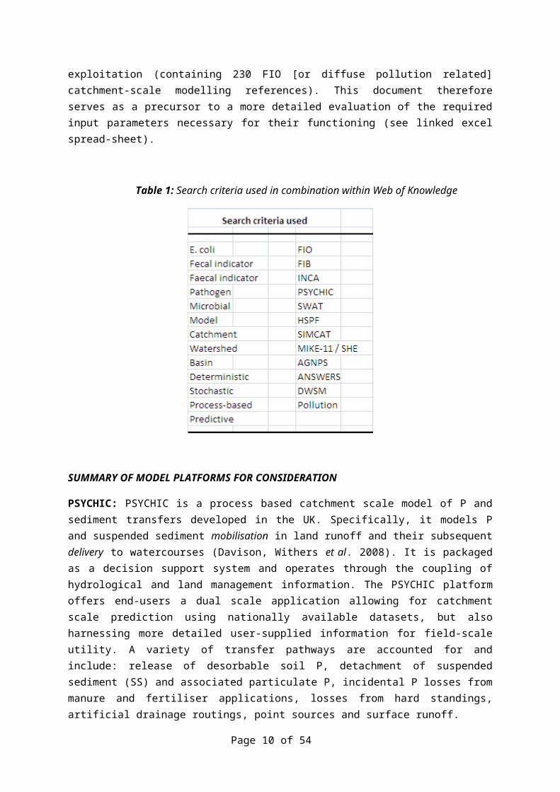
There are a considerable number of model platforms from around the world and the following text provides a brief summary of those identified as having greatest potential for further development with regard to microbial prediction. Web of Knowledge was the principal engine for the literature search using combinations of key words as shown in Table 1. This text summary has been condensed into two accompanying Excel summary tables for each model and an initial reference bank has been created within Endnote for further exploitation (containing 230 FIO [or diffuse pollution related] catchment-scale modelling references). This document therefore serves as a precursor to a more detailed evaluation of the required input parameters necessary for their functioning (see linked excel spread-sheet).

Page 6 of 37

Table 1: Search criteria used in combination within Web of Knowledge

SUMMARY OF MODEL PLATFORMS FOR CONSIDERATION

PSYCHIC: PSYCHIC is a process based catchment scale model of P and sediment transfers developed in the UK. Specifically, it models P and suspended sediment mobilisation in land runoff and their subsequent delivery to watercourses (Davison, Withers et al. 2008). It is packaged as a decision support system and operates through the coupling of hydrological and land management information. The PSYCHIC platform offers end-users a dual scale application allowing for catchment scale prediction using nationally available datasets, but also harnessing more detailed user-supplied information for field-scale utility. A variety of transfer pathways are accounted for and include: release of desorbable soil P, detachment of suspended sediment (SS) and associated particulate P, incidental P losses from manure and fertiliser applications, losses from hard standings, artificial drainage routings, point sources and surface runoff.

A number of caveats are apparent when PSYCHIC is operated at the catchment scale. For example, the model is not programmed to account for bank erosion as a contributor of P loading (nor in-stream processing of P for that matter). PSYCHIC uses a monthly time-step and the spatial scale of operation allows for the accumulation of 1km2 (or smaller where possible) spatial data that the model combines with management information derived from Ag Census returns and relevant survey responses.

As with any process-based model PSYCHIC has a number of data requirements in order to function. These are outlined briefly in the following list (though a considerable number are considered practical constraints on uptake of PSYCHIC as a modelling platform of choice, largely because of licensing issues):

1. Manure Management Database (held by ADAS), combining agricultural census data with the survey of fertiliser practice;

Page 7 of 37

2. MAGPIE (held by ADAS): used in PSYCHIC as a database of land use type, the number of livestock per ha of managed grass and the proportion of each crop grown per ha;

3. NATMAP (held by NSRI): series based, 1km2 spatial data set of % coverage of each soil series;

4. National Soil Inventory (held by NSRI): physical properties associated with each of the soil series under different land use conditions;

5. HOST (Held by CEH/NSRI): Classification of the soils of the UK;6. DEM;7. Census data (no of people per km2);8. Climate Surface (held by Climate Research Unit, UEA) – climate attributes including

rainfall, rain days, wind speed, sun hours, maximum temperature, minimum temperature;

9. Drainage density (river network; CEH);10. Index of proximity to surface water (connectivity).

Clearly, a number of datasets are the property of research institutions and or consultancies and the model code itself is held by ADAS and is not open access. The EA do have a PSYCHIC 1 version (Neil Preedy is the contact at the EA who would know such details)1.

The main model components include modules that account for: water balance and hydrological pathways (using the mean climate drainage model [MCDM]); sediment loss (using the modified Morgan-Morgan-Finney Model); incidental losses (determined by rainfall intensity and cumulative rainfall since application); solubilisation of P in soil (a function of soil Olsen P); Particulate P loss with eroded sediment (including an account of particle size distribution effects); and delivery as determined by hydrological connectivity (which strictly speaking is transfer potential rather than deliver (Beven et al. 2005). The PSYCHIC model can therefore be divided into a combination of processes governing water balance and those governing mobilisation and delivery. Values for surface and subsurface flow volumes associated with each of the land use classes are derived using the MCDM. An area weighted approach is then adopted to obtain the overall proportion of different flow pathways in each grid cell, and the relative importance elucidated via reference to soil properties. In the end the assigning of the importance of those pathways will depend on what processes you want to represent and what information will be available to constrain/evaluate those processes. The final model can then be run including uncertainty bounds. PSYCHIC makes inroads in attempting to account for hard standings as key contributors to SS and P inputs to streams and uses hydrologically effective rainfall (HER) as a factor in determining their importance. The model architects note that more work is needed to develop this element (Davison, Withers et al. 2008). Similarly, in attempting to include septic tank inputs within the PSYCHIC framework the ‘educated guess’ of particular proportions of the population being connected to mains sewers is again recognised by the model architects as a weakness in design. As a final point, the application of the prototype PSYCHIC model has been linked to feedback from catchment dwellers and stakeholders. Such local knowledge ensured that predictions provided by PSYCHIC could be fine-tuned and reality-checked (Collins,

1 The project team needs to identify whether the EA have the code or just an executable version (probably the latter) – we would need to consult with Neil to determine what exactly we could vary. If we don’t have the code we cannot add an FIO component without going back to ADAS – speak with Neil. [Louise: We will not have access to the code].

Page 8 of 37

Stromqvist et al. 2007) though this can be difficult to obtain when models are transferred to other catchments unless community engagement is already well established.

Potential to consider as microbial modelling platform?: WEAK, largely because of monthly time-step approach and complex licensing issues and access to original code – though discussion with EA is perhaps needed on this. The monthly time-step must be considered as too low a resolution for prediction of contaminants that are so heavily dominated by incidental surface-driven losses. The lack of accounting for bank erosion is not a major limitation for FIOs though the omission of in-stream processing capability could be problematic given the likely range of differential die-off and resuspension rates of FIOs and particle-bound FIOs within the water column and stream bed sediment. An additional bolt-on model could be feasible. The attempt to include hard-standing contributions of diffuse pollutants is of high interest in terms of transferability to FIO modelling though the robustness of the hard standing component is questionable. This is because HER is coupled with a number of additional coefficients that are essentially preliminary estimates. Also, it is perhaps more favourable to discount models that operate using 1km2 grids. Instead, model platforms that use HRUs could designate catchment Critical Source Areas (CSAs) as the most important HRU. 1 km grids are often used for other reasons - commonly because data is often available in GIS grid-based format and therefore convenient but the best model is not necessarily grid-based. More realistic and logical, but slightly harder to deal with, is the delineation of a catchment into CSA and non-CSA areas (e.g. PEDAL2) or HRUs or Functional Units (FUs) (e.g. SWAT, eWATER). Beyond this issue we also need to query the appropriate spatial scale for some of the transfer pathways and sources e.g. hardstandings, where a very detailed scale me be crucial for these known hot-spots.

An interesting comment on PSYCHIC (with generic applicability to other models) can be drawn from information published in the final report to Defra (2005) whereby a number of questions were raised in terms of the usefulness of the UK Environment Agency (EA) data archive. Load estimates based on EA data were actually shown to be unreliable with significant bias and imprecision and to circumvent this weakness, it was apparent that testing of model outputs should be undertaken with targeted and detailed monitoring of flow, SS and P (Defra, 2005). While the likelihood of PSYCHIC being recommended as a modelling platform suitable for FIOs is rather low given a number of limiting factors already identified, this point does raise a generic point of utmost importance that will be a general concern for any modelling platform. For FIOs, in-stream empirical fate and transport data is extremely limited but would be needed to parameterise process-based FIO models at the catchment scale. This brings issues of specific model evaluation requirements to the fore. Clearly, a means of testing and evaluating modelling capability within reliable data constraints is vital to ensure any degree of confidence in model outputs. Interestingly, the final report to Defra recognised that the ‘integration of current understanding of sediment and P loss risk into reliable quantitative predictive models is less well advanced than for nitrate’. This is an important statement that is magnified when applied to the existing FIO evidence base. This reinforces the policy need for enhanced water quality monitoring programmes (potentially via the DTC projects) to provide measured data with which to evaluate FIO load estimates.

Page 9 of 37

INCA: The INCA model is a process-based, dynamic, semi-distributed and integrated catchment model. It is highly parameterised and therefore requires a large number of input variables some of which are poorly understood and others which are deemed to be impossible to measure (Dean, Freer et al. 2009). Essentially, INCA is a dynamic mass-balance model designed to provide a process based representation of plant/soil dynamics, instream biogeochemistry, hydrology and the fate and distribution of chemicals in aquatic and terrestrial environments. The platform simulates water flow and associated water quality and attempts to track hydrological flow pathways operating in both the land and riverine phase. Its dynamic nature means that day-to-day variations (i.e. changes in daily mean values) in flow and water quality are included for both the land and stream phase components. The nature of the model is such that changes in land use or climate on water flow and associated quality can be simulated. The approach is one whereby a simple mixing model is applied to water and contaminants of interest linked to different land uses (up to 6 user defined classes) within each reach and the resultant is then routed along the main stream. It is important to note the semi-distributed nature of INCA and to not confuse it with a fully-distributed model. The purpose of the INCA platform is not to model catchment land surface in explicit detail. Instead different land use classes and sub catchment boundaries are modelled simultaneously with output from these different spatial components providing subsequent input data for a multi-reach river model. The hydrological land-use model component of INCA is driven by a daily mass balance and facilitates the calculation of daily water flows for soil, groundwater and leaching to the river system for up to 6 land use classes using a daily time step.

The river model component uses conventional non-linear reservoir dynamics to simulate the routing of water down the river network. Therefore, the river model operates in a similar manner to that associated with ANSWERS, ANSWERS-continuous and HSPF (see later descriptions) to route water down the river system. In addition to solving flow equations, there is a requirement to solve NO3-N and NH4-N mass balance equations in soils and groundwater zones.

The INCA platform is complex. It has to be because it attempts to describe a large number of factors and processes in the catchment environment. Such modelling philosophies are limited by the availability of sufficient and reliable data even for small catchment areas (Dean, Freer et al. 2009). The model platform was originally developed to predict daily time series of soil-water NO3 and NH4 concentrations and fluxes (including temporal variations in flow paths and N transformations) (Wade, Whitehead et al. 2002). A full model description is presented in Whitehead et al. (1998).

Briefly, the hydrological model is constructed from three component parts, namely: (i) MORECS – the Met Office rainfall and evapotranspiration calculation system (converting rainfall into HER to drive water transfers); (ii) a system allowing simulation of the effects of the land surface on flow (using a two-box approach whereby principal reservoirs of water are deemed to be the reactive soil zone and groundwater); and (iii) river flow model (based on mass balance of flow as discussed above) (Whitehead, Wilson et al. 1998). N inputs to each subcatchment are derived from land use and DTM data. Land use is also used as an approximate surrogate for soil type for a number of characteristics that can influence N transformations.

Page 10 of 37

In 2002 Wade et al. published an updated version of INCA. The general structure remained largely unchanged and so the equations are still founded on the 4th order Runge-Kutta technique enabling simultaneous solution of model equations. This in turn ensures that no process representation within the model is able to take precedence over another. What did constitute a major amendment was the inclusion of retention volumes. Thus, the simulation of long term changes in water and N stored in soil could be simulated and this removed the previous oversimplification whereby water storage volume within the catchment depended only on the rainfall input. The corresponding soil drainage volume stored in the soil could now respond rapidly to water inflow – and could be conceptualised as macropore, drain or piston flow and impact on the rising limbs of hydrographs. Conversely, the soil retention volume represented the proportion of water in the soil that responds much more slowly and is comparable with the field capacity concept (and water associated with soil micropores). The other notable changes were the conversion of process equations to be represented in terms of loads rather than concentrations and that a fertilizer submodel was removed and replaced with a daily-timeseries of mass inputs from an additional read-in file (allowing for multiple fertiliser applications within a single year). Example catchment applications of the N version INCA are available (e.g.(Jarvie, Wade et al. 2002; Rankinen, Lepisto et al. 2002).

A number of versions (in various degrees of development) of INCA are discussed in the literature including INCA-N (flow, nitrate and ammonia), INCA-P (flow, TP,DP, PP, macrophytes), INCA-SED (flow, sediment including size fractions, stream power, shear velocities), INCA-C (DOC, DIC, Particulate C), INCA-metals (flow and metals) and INCA-Trit (for radioactive pollution events). There is no FIO version of the INCA platform. INCA-P is considered here as an example of extension of the INCA modelling philosophy. INCA-P evolved as a platform to model the transport and retention of P in terrestrial and aquatic environments, and to simulate bed sediment resuspension and suspended sediment deposition. There are three key components of INCA-P (according to (Dean, Freer et al. 2009)): (i) land phase hydrological model; (ii) land phase P model; and (iii) in-stream P model (an in-stream processing component would be useful for FIO modelling). These three components calculate discharge through different pathways, P stores and transformations in soil and groundwater and P processes operating within the stream, respectively. The land-use hydrological model provides a daily mass balance of water flows at a daily time step.

Data describing typical land management practices (grazing season duration, application timings and quantities etc) are required. The key assumptions made are that fertiliser, wastewater and manure inputs are equal across a particular land use class, irrespective of geographical positioning within a catchment. Similarly, the P process rates are the same irrespective of catchment location, though can still vary according to spatial variations in soil moisture and temperature and finally initial stores of P and water associated with each land use class are the same irrespective of location within the catchment (Wade, Durand et al. 2002). These assumptions are basically included as an attempt to simplify the model complexity (though given the structure and parameter requirements this does not mean that the model itself is particularly simple). In fact, INCA-P is more complex than INCA because the controls on catchment scale P transport require considerations of P adsorption on sediments and subsequent sediment associated transfer within stream systems (Neal, Whitehead et al. 2002). To demonstrate the complexity of the model structure there are 93 parameters to populate if the system is treated homogeneously. The application of the model

Page 11 of 37

to the River Lugg catchment, as an example, required 901 parameters to cover 22 stream reaches and 6 land use types.

Potential to consider as microbial modelling platform?: WEAK, largely because it is so complex, but the in-stream component could be of interest. However, this would depend on where the similarities lie for in-stream processing on chemical versus microbiological pollutants because it may be that FIOs require a completely different approach. For INCA-P it is important to note that recommendations following applications to different catchments have suggested a need to obtain detailed point source data and a more general assessment of relative contributions of point and diffuse sources (Dean, Freer et al. 2009). Critically, the current monitoring networks of the EA are not yet sufficient to meet this need.

SCIMAP: First and foremost it is important to stress that Scimap is not considered a water quality model (c.f. Simcat). However, nor is it a conventional rainfall-runoff model. Instead Scimap operates in order to inform model-users where in a particular catchment you have tributaries, fields or parts of fields that are producing risk. Essentially, it is a tool to prioritise where to take action in a catchment, and is termed a risk-based’ model, so is not a process-based platform. Scimap uses a high resolution DEM and landcover map to profile where the risks are most likely to be and therefore only uses readily available data. A strong advantage is that it is open (controlled) access, meaning it is open access without charge but the output could be used incorrectly so the model architects keep abreast of who is using it and for what purpose. Scimap has been developed to predict fine sediment risk, P risk and is starting to develop N risk (to an extent). While Scimap only looks at relative risk within a catchment rather than absolute risk between different catchments there are modifications for Scimap P and N to provide absolute results and any relative model could be calibrated to give some absolute results.

The underlying hydrological concepts of SCIMAP are based upon digital terrain analysis. SCIMAP couples the a/Tan(beta) concept that provides a soil wetness propensity index (a = uphill contributing area, and beta is the local slope angle: which underpins the TOPMODEL approach) and a Network Index (a surface flow connectivity index explained further below) to provide a risk map for the connectivity of surface flows that can be linked to diffuse pollutants (Reaney et al., in press; Lane et al., 2010). Within SCIMAP, routing of overland flow is accomplished by assigning a travel time value to each cell. Travel time is calculated by accumulating distance from the outlet to the source (by tracing back along the direction of steepest slope) and dividing by the flow velocity. Second, connectivity is handled using the concept of a network saturation value. The network saturation value of a source cell is the lowest saturation value on the flow path to the channel. When the network saturation value reaches a threshold, the source cell is connected and overland flow can occur. Each cell therefore has three attributes: local saturation value, network saturation value and travel time. These attributes are the basis for a new definition of hydrologically similar zones.

Potential to consider as microbial modelling platform?: MODERATE to HIGH as a risk-based tool, but clearly WEAK for process based model. The project team need to engage with end-users to determine appropriate needs for FIO modelling. Some discussion surrounding the linkage of the SCIMAP model to the PEDAL model (for P)

Page 12 of 37

has been taking place between Lancaster and Durham and this represents a potentially useful development if SCIMAP could be extended to FIOs. The discussions are based upon the possibility that PEDAL can be used to identify absolute diffuse pollution risk “hotspots” at the headwater catchment scale and SCIMAP then used to map the relative risk of different areas within a given catchment.

PEDAL2: [Note potential conflict of interest as four members of the project team are involved in the PEDAL2 project – needs to be borne in mind]: The PEDAL2 project is a continuation of Defra funded research into a modelling platform to predict the delivery of P to watercourses using a decision-tree approach. The platform makes use of national coverage data held within GIS at the 1km2 scale. This combines with a ‘field toolkit’ of measurements and qualitative observations.

The scale of operation of PEDAL is the headwater catchment scale and it is being developed to predict delivery of P and FIO to headwaters draining small catchments. There would need to be a linkage with other modelling platforms to enable subsequent routing and in-stream processing of E. coli loading through stream networks of any larger catchment, or a targeted campaign of measurement of instream effects. Furthermore, PEDAL is specifically designed to account for the diffuse signal of P and FIO contributions to surface waters, it therefore does not consider point source inputs nor in-stream processing or direct deposition to streams by livestock, although some of these factors are implicitly included in the delivery coefficients calculated as they cannot always be separated.

The PEDAL2 modelling platform differs considerably from applications such as SWAT and HSPF (see later descriptions) largely because the PEDAL philosophy is to use fewer model parameters to constrain uncertainty in model output. The ultimate aim of the PEDAL approach is to attempt to identify whether mitigation measures aimed at the control of sources, mobilisation or delivery (or a combination of these) of pollutants is likely to be more effective. Quantifying the actual amount of pollutants such as FIOs and P delivered to waterbodies is challenging owing to the variability of factors that affect their mobility and transport. We have increasing scientific knowledge of these factors at smaller experimental scales but we still do not have reliable general rules that can predict delivery of pollutants at larger scales such as catchments and river basins that are often used operationally by regulatory bodies. The PEDAL project has provided scale-dependent estimates of P delivery from headwater catchments to water courses using simple physical drivers of P transport (i.e. rainfall, hydrological soil classification and connectivity to local watercourse). This has been done using a decision tree approach. The approach was calibrated to delivery coefficients observed at project catchments (i.e. using a measure of annual P loss divided by the DESPRAL measure of mobilisation: PE0106). The delivery coefficient estimates produced were expressed such that predictions reflected the associated uncertainty, rather than a single number. These initial delivery coefficient ranges were modified by structured catchment visual assessments (VAs) that identified whether land management, land boundaries and/or land use, for example, would increase or decrease the likely magnitude of P delivery: this was quantified into a catchment VA score. The modelling structure proposed for the FIO component of PEDAL2 focuses on identifying physical FIO loss by estimating delivery of FIOs to headwater streams. PEDAL2 facilitates this by estimating FIO delivery as a ratio of the observed FIO loss to FIO sources using a similar

Page 13 of 37

fuzzy decision tree approach to PEDAL. However, there are few existing studies on the magnitude and dynamics of catchment FIO sources (c.f.(Coffey, Cummins et al. 2010; Coffey, Cummins et al. 2010) for SWAT) or field FIO survival studies. The FIO model is currently being developed in a similar manner to the P model with an expert workshop for evaluation of model structure, development of an FIO VA and a farmer questionnaire and identification of fuzzy rules for predicting the effects of mitigation measures on FIO sources and delivery coefficients. Ideally, the focus of a predictive model would be to determine FIO fluxes at hydrological event-scale as these timescales are the key requirement of the policy community (Kay, Edwards et al. 2007). However, this is a very difficult task given the limited high resolution data that exists from previous studies (to date few studies have measured FIO dynamics through events to facilitate model evaluation: (Kay, Edwards et al. 2007)). Given the storm-event focus of PEDAL, the project team will obtain delivery coefficients at hydrological event scale, which is a temporal disaggregation of export coefficients.

Once delivery coefficients have been determined for monitored sites the model will be used to provide fuzzy estimates of sources and delivery from national scale data on land use, farming practices and catchment physical characteristics. As with the P model, the VA and farmer questionnaire can be used to refine these estimates at locations of interest. The new PEDAL model structure has been calibrated on existing P data because at current time the project does not have a full year’s data yet from the new catchments. A GUI is to be developed in accordance with EA/Defra wishes as agreed at the June 2010 steering group meeting.

The model code will be provided to Defra and the EA. All output from the project will be jointly owned by DEFRA and the research consortium and will be made available to potential users provided they receive sufficient training in the use and potential limitations of the models developed, the field methodologies and the modelling results. This is comparable with say TOPMODEL whereby it is free for academic use, but not free for consultancy. So for PEDAL, project team and / or Defra can decide who can use it.

Potential to consider as microbial modelling platform?: WEAK in considering applicability to process-based modelling at catchment scale; MODERATE TO HIGH (given already considering FIOs) for a sub-component of a larger FIO modelling platform but like SCIMAP the package is not useable as a stand-alone. It could help inform catchment modelling aspects but does not account for point sources or in-stream impacts. Lack of accounting for point sources does not rule out the PEDAL model as a contender platform but instead highlights the need to clearly define the purpose of any FIO model to determine appropriate development needs. Issues such as those raised have already been brought to the fore at a recent PEDAL FIO expert workshop which was conducted, in part, to highlight future development needs for improvement and uptake of the PEDAL2 model.

MHtracking Modelling @ Newcastle University: In a 2007 review paper O’ Connell et al. (2007) refer to the tracking of ‘impact information’ through a catchment via a modelling approach. The underlying concept is to track ‘packets’ of water from source areas to a site of impact (using a pixel-based approach) via routing through the stream network. The model has been developed primarily for flood prediction (see FRMRC2 project) but clearly the approach offers potential for application to pollution prediction and tracking.

Page 14 of 37

The general philosophy for the distributed Mass and Head tracking (MHtracking) models developed at Newcastle is that a complete understanding of the water flows and water quality downstream in a river catchment is possible only if high-quality space-time modelling is used that allows hydraulic head and the various masses of water, solute, sediment and ice to be tracked all the way through the catchment, starting from source locations. Head and the various masses move at different space-time-varying speeds and the accurate prediction of impacts downstream depends on getting these speeds approximately correct. Even in the simplest possible simulations where a secondary mass such as solute is carried freely with water the time-varying impact on the water quality downstream depends to a large degree on the relative speeds of the hydraulic head and the bulk water velocity.

This approach has been a long time in development, starting in the mid-1990s using the SHETRAN physically-based spatially distributed modelling system (e.g. using solute species as a label to track sediment from different source locations, (Ewen, Parkin et al. 2000)). It has evolved considerably over the years, partly in response to an improved understanding of the fundamentals of tracking but also an understanding of the limitation of field data, such as the inadequacy of DEMs as a basis for the prediction of the downstream impact of hot-spot (point, or limited area diffuse) pollution. Fine-scale grid nesting, where fine grids are nested within coarse grids to allow attention to focus on important locations in the catchment, is possible in a new (unpublished) version of SHETRAN that was developed and used for the nuclear industry, but even this is not completely satisfactory when working with very small hot spots.

One positive consequence of the evolution has been the adoption of a modular modelling approach, to create a suite of MHtracking models, so that different models are used to meet the various demands for modelling source areas, runoff generation and channel networks. There are four classes of models: (1) the classic integrated approach, e.g. using SHETRAN; (2) adjoint models for studying the propagation of mathematical derivatives, to give insight into the sensitivity of downstream impacts to upstream causes (this has been applied to various models (e.g. (Ewen, O'Donnell et al. 2010)); (3) mass tracking over the top of distributed water flow model, including tracking particles and packets (e.g. (O'Donnell 2008; Geris, Ewen et al. 2010)) ; and (4) tracking in which the fundamental model is a tracking model (e.g. the types of approaches used in Ewen (2000) and (1996) where water mass is treated as particles and water packets).

The MH tracking approaches allow the various dispersion effects to be represented explicitly and their consequences to be analysed.  These include hydrodynamic and geomorphologic dispersion of head and the dispersion of the various masses, including dispersion associated with instream variations in water flow velocity (i.e. variations across cross-sections, around the bulk mean velocity), settling velocities and mass-mass interactions.

The various MHtracking models are distributed and use either (or a combination of): regular grids, nested grids, dendritic networks, or free-form polygon grids (e.g. customised grids that can accommodate linear features such as sheep pathways, moorland grips, and roads). They work with fixed time steps of appropriate size (e.g. 5 minutes or 2 hours) and typically simulate several years.

Fundamentally, the MHmodels are physics based and use data that fully define the various structures and media for the region being modelled. The demand for data depends on the

Page 15 of 37

scope and ambition of the study. The basic data are time series for rainfall and potential evaporation. Most of the models require a DEM, to be used as a starting point for the network and grid creation. The other requirements depend on the model and problem, but can include, for example, survey data for hot spots, survey data for channel geometry and vegetation, and national data sets for land use, soils, etc. One of the main purposes in developing the MHtracking models is to study the impact of changes in land use/management and climate. Models within MHtracking can represent transport in surface and subsurface waters, adsorption to sediment with in-stream deposition and remobilisation, and solute decay. Both diffuse and hot-spot sources can be represented.

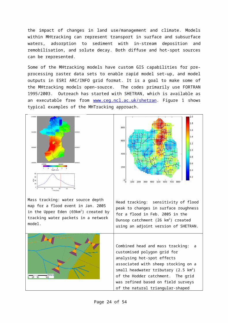
Some of the MHtracking models have custom GIS capabilities for pre-processing raster data sets to enable rapid model set-up, and model outputs in ESRI ARC/INFO grid format. It is a goal to make some of the MHtracking models open-source. The codes primarily use FORTRAN 1995/2003. Outreach has started with SHETRAN, which is available as an executable free from www.ceg.ncl.ac.uk/shetran. Figure 1 shows typical examples of the MHTracking approach.

Mass tracking: water source depth map for a flood event in Jan. 2005 in the Upper Eden (69km2) created by tracking water packets in a network model.

Head tracking: sensitivity of flood peak to changes in surface roughness for a flood in Feb. 2005 in the Dunsop catchment (26 km2) created using an adjoint version of SHETRAN.

Combined head and mass tracking: a customised polygon grid for analysing hot-spot effects associated with sheep stocking on a small headwater tributary (2.5 km2) of the Hodder catchment. The grid was refined based on field surveys of the natural triangular-shaped severe soil compaction zones that develop at river-crossing points. All the coloured elements are part of the grid, including the linear blue elements that comprise the drainage network and the thin orange

Page 16 of 37

elements that comprise the sheep tracks.

Figure 1: Typical examples of distributed Mass and Head tracking (MHtracking): provided by Greg O’Donnell

Potential to consider as microbial modelling platform?: MODERATE TO HIGH as the modelling approach scores positively in terms of the key criteria listed in earlier sections of this report. The hydrological modelling forms a key component of the model and its ability to operate at high resolution time scales is important for FIO response to storm events. The ability to account for flow via different pathways and in-stream sedimentation and resuspension is of benefit for transferability to account for FIO dynamics in catchments, as is the ability to account for particle adsorption and contaminant decay.

MIKE SHE: MIKE SHE (Refsgaard, Storm et al. 1995) is a watershed-scale physically based, spatially distributed model for water flow and sediment transport. This modelling platform emerged in the 1980’s and has been developed and extended by DHI Water & Environment ever since.

MIKE SHE uses MIKE 11 to simulate channel flow. Flow and transport processes are represented by either finite difference representations of partial differential equations or by derived empirical equations. The following principal submodels are involved:

1. Evapotranspiration: Penman-Monteith formalism2. Erosion: Detachment equations for raindrop and overland flow3. Overland and Channel Flow: Saint-Venant equations of continuity and

momentum4. Overland Flow Sediment (and WQ parameter) Transport: 2D total sediment

load conservation equation5. Unsaturated Flow: Richards equation6. Saturated Flow: Darcy's law and the mass conservation of 2D laminar flow7. Channel Sediment Transport 1D mass conservation equation.

This model can analyze effects of land use and climate changes upon in-stream water quality, with consideration of groundwater interactions, and is able to simulate both event driven episodes alongside longer-term continuous hydrology and water quality responses in catchments. A grid network represents spatial distributions of the model parameters, inputs, and results with vertical layers for each grid.

Lumped parameter conceptual models (e.g. SWAT, INCA, HSPF) are an attractive alternative because they are easier to operate and require less data. However, critics of lumped conceptual models will argue that their predictive capability with respect to assessing

Page 17 of 37

the impacts of changing management practices is questionable due to the semi empirical nature of the process descriptions (Hansen, Refsgaard et al. 2007). The MIKE SHE modeling system is proprietary software, owned and distributed by DHI. The software must be purchased from DHI. It is worth noting that in an comprehensive review of modelling platforms Merritt et al. (2003) state that the predictive capability of MIKE-11 (part of the DHI Mike model suite) is undermined by several factors. The most striking referred to by these authors is that Mike-11 opts to use one-dimensional equations to represent three-dimensional processes and as a consequence major simplifications of critical interactions are made, or worse still ignored completely.

Potential to consider as microbial modelling platform?: WEAK, based on the fact that it is overly complex and can be overparameterised for simpler applications such as predicting catchment outlet discharge. In many cases some of the parameters are simply not available. A clear criticism of MIKE-SHE is that it is extremely intensive in terms of computational requirements and that this can inhibit its uptake and application for large catchments where its use simply becomes too inefficient. As noted by Jakeman et al. (2006) - Model structures with too many parameters are still endemic. A compromise between physically-based complex models and black box approaches could be represented better by lumped parameter models. MIKE-SHE is not freely available and data requirements can be prohibitive in terms of costs.

SWAT: SWAT is a basin scale, physically-based, continuous time distributed parameter model capable of operating on a daily time-step. The model code and structure originated from the USDA-ARS with the intention of providing long-term yield predictions. It can accommodate a large number of parameters but of course not all parameters are common to all catchments. It is a direct descendent of the Simulator for Water Resources in Rural Basins (SWRRB) model. The SWAT architecture has undergone continued evolution and extension since the 90’s (Gassman, Reyes et al. 2007). SWAT does not adopt a mass-balance equation approach for routing water through catchment systems and instead opts to maintain water balance by accounting daily or sub-daily water budgets and uses an empirical procedure to route the water through channels. Reference is also made to the Runoff Curve Number method to determine runoff volumes.

The model structure allows for basins to be subdivided into watersheds which are then broken down into unique hydrological response units (HRU’s). Each sub-basin should accommodate between 1 and 10 HRUs. Implicit to the concept of HRUs is the assumption that no interaction occurs between HRUs in any given sub-basin. Load exports from each HRU are calculated separately and then summed for each sub-basin. SWAT will only allow for spatial relationships to be developed at the sub-basin level. A common procedure within SWAT is to simulate the land phase of the hydrological cycle and thus determine pollutant loadings to the main drainage channel, with a subsequent modelling of the movement and transformations occurring within the channel during passage through the subbasin. Within SWAT bacteria are added to HRU’s at a rate specified by the model user (Chin, Sakura-Lemessy et al. 2009). This input rate can vary over time and is determined as the product of the bacteria content of manure and manure loading rate which can be constant or vary on a day-to-day basis. SWAT partitions bacteria into either soluble or sorbed phases using a

Page 18 of 37

linear isotherm approach. SWAT also requires that any subsurface FIO contributions to receiving waters are regarded as zero which is a considerable limitation given, for example, the reported potential for preferential flow transport of bacteria (Chin, Sakura-Lemessy et al. 2009). A preliminary assessment of the SWAT model at a more coarse timestep (monthly) was undertaken with regard to Cryptosporidium modelling (Coffey, Cummins et al. 2010). It is important to stress the absence of observed water quality monitoring data and need for extensive input data for Cryptosporidium in this catchment study and so the reported study was only considered as an initial step in model development with no calibration or validation (Coffey, pers comm.). Others have explored the development of an hourly timestep within the SWAT framework, including the Enhanced Soil & Water Assessment Tool (ESWAT) (Debele, Srinivasan et al. 2009) and more recently sub-hourly time-steps for rainfall-runoff modelling within SWAT (Jeong, Kannan et al. 2010). A detailed breakdown of SWAT parameter needs and a summary of applications are presented in Excel spreadsheet 2.

SWAT is able to accommodate changes in management practice. The model structure is such that the following can be simulated: (i) terracing; (ii) tile drainage; (iii) contouring; (iv) filter strip provision; (v) strip cropping; (vi) fire; (vii) grassed waterways and (viii) change of specified plant type. Modelling long term water quality impact of BMPs using SWAT is reported in Bracmort (2006) and Tuppard et al. (2010). Land use change can also be included as a management change. Critically, as noted by Borah et al. (2007), SWAT is not capable of detailed, single event flood routing because it operates on a daily time-step. A sub-daily time-step is required for high detail event modelling (e.g. HSPF, AGNPS, ANSWERS, DWSM). However, this means that it is better suited to predicting long-term effects of hydrological fluctuations and management practices.

The concept and need for a microbial submodel within SWAT was first raised by Sadeghi and Arnold (2002). Consequently, Swat2005, a later version of the model, has several significant enhancements; the most significant with respect to this review is the inclusion of bacteria transport routines (Arnold and Fohrer 2005). However, Benham et al (2006) comment that SWAT, as well as HSPF, have limited flexibility and options; the model does not have much capacity to account for bacterial life cycles or simulate bacterial concentrations in extreme conditions. More recently, Kim et al (2010) report on SWAT2005 and the bacteria transport routine within which bacteria die-off is the only in-stream process. Kim et al. (2010) presented details relating to the development of the partial model of sediment associated bacterial transport to evaluate the significant of the bedload store of E. coli, and subsequent release. Likewise, Parajuli et al. (2009) provide details of refinements to SWAT 2005 in their source characterisation of faecal bacteria and sensitivity analysis of SWAT2005. Specifically, they assessed the sensitivity of the following user-defined parameters: (i) bacteria soil partition coefficient in surface runoff; temperature adjustment factor; less persistent bacteria die-off in solution phase; less persistent bacteria die-off in sorbed phase; and bacteria partition coefficient in manure, and one input parameter, - faecal coliform bacteria concentration in manure. Their use of the model allowed for spatial faecal inputs relating to confined animals, grazing, failing septic tanks and wildlife. The bacteria soil partition coefficient in surface runoff had the greatest sensitivity and the authors cautioned users to select locally relevant data for this parameter.

Coffey et al. (2010) demonstrate the development of a pathogen model using SWAT and the microbial submodel. As per SWAT requirements input data regarding agricultural practice,

Page 19 of 37

demographics and hydrological parameters was used. Importantly, the Coffey paper identified key areas where future research is needed in helping define input data – a key requirement was found to be the initial concentration of E. coli in human / animal waste. Sensitivity analysis of the bacteria subroutine provides a key insight to the important parameters needed to parameterise the model for the river Fergus Catchment. The role of temperature on cell die-off and the bacterial partition coefficient were both found to be most sensitive parameters whereas initial concentration of E. coli in faecal material of both human and animal origin was determined to be the most significant realtime variable. Coffey et al. (2010) propose that the ‘ideal catchment model’ should be capable of simulating four specific factor categories: (i) land use factors; (ii) climate factors; (iii) topographical factors; and (iv) hydrological factors. Data requirements are listed in the accompanying spreadsheet. [are these less sensitive that hydrology though – probably, because mobilisation is likely to be more sensitive. Sensitivity analysis on microbial submodel alone is not so important – double check]. Other recent developments include the coupling of SWAT with MARS-2D for microbial predictions in downstream estuaries (Bougeard, Le Saux et al. 2010).

Potential to consider as microbial modelling platform?: MODERATE - HIGH, given microbial submodels are already in development, freely available and able to operate at a range of timesteps, including a daily (it is an averaged daily value) and hourly timestep. The SWAT platform has evolved considerably probably because of its public domain status which has allowed numerous modifications and refinements (e.g additional water quality parameters, finer resolution timesteps etc.). The option to use a monthly time-step seems inappropriate because it appeared to bring about unexpected (and underestimated) predictions of Cryptosporidium in the Coffey study but clearly finer resolution time-step options are available. Reference to spreadsheet 1 indicates that a high number of the ‘key indicators’ are satisfied for taking this modelling platform forward.

HSPF: HSPF is a conceptual, lumped parameter model that was first publicly released in 1980 (Johanson, Imhoff et al. 1980). It was developed by the USEPA and simulates for extended periods of time the hydrology and associated water quality response to land surfaces and in-stream processing. It uses continuous rainfall and other meteorological records to compute streamflow hydrographs and pollutographs and can therefore produce a time history of water quantity and quality at any given point in a catchment. HSPF simulates interception soil moisture, surface runoff, interflow, baseflow among others. The model contains hundreds of process algorithms developed from theory, laboratory experimentation and empirical relations from instrumented catchment studies. HSPF is able to accommodate a timestep of <1 day and therefore is well suited to the simulation of specific events. In the study of Chin et al (2009) which compared output of SWAT and HSPF it was noted that HSPF provided higher performance in terms of predicting daily flows, a direct effect of the higher resolution time-step. That said, Borah and Bera (2007) acknowledge that HSPF is not adequate for simulation of intense single events, especially in large catchment areas because it is not able to reliably represent single-event flood waves. Interestingly, for the prediction of bacteria concentrations at a catchment outlet, Chin et al (2009) found that SWAT outperformed HSPF suggesting that the bacteria fate and transport processes used within SWAT provide a better representation of catchment activity (though how transferable

Page 20 of 37

such a finding is outside of the study catchment used here is uncertain). For the daily timestep FIO concentrations are averaged to give the daily output. The hydrological process equations within HSPF are therefore fundamentally different from those used within SWAT. However, as with ANSWERS and ANSWERS-continuous this modelling platform uses a simple storage-based (non-linear) reservoir equation to determine flow routing within the catchment.

Essential data requirements for HSPF include:

1. Meteorological records of precipitation and estimates of potential evapotranspiration2. Water quality simulation needs tillage practices, point source inputs, application info

For microbial prediction it is FIO source loads which are essential input parameters and accurate estimation of these loads is extremely important for good model performance using HSPF (Zeckoski, Mostaghimi et al. 2003). In fact, both daily and hourly faecal coliform loads from direct deposition to streams and from deposition on various land use types are required by the HSPF platform. Direct deposition data is required in a time-series format and land application via a tabular format. Zeckoski et al (2003) have developed a FIO calculator to provide input data for HSPF that is written in visual basic and outputs using Excel spreadsheets. This calculator component requires information on livestock numbers, stream access and land use.

The processes describing FIO fate and transfer are fundamentally different in HSPF from those in SWAT leading some to suggest that a reduction in model structural uncertainty could be achieved by using multi-model approaches (Chin, Sakura-Lemessy et al. 2009). In HSPF the bacteria loading rate to land is specified directly by the model user and can take the form of a constant or be varied monthly. HSPF allows for transport of FIOs either via direct entrainment within overland flow or by association with sediment. HSPF, in contrast to SWAT, allows for subsurface contributions of FIOs to streamflow via throughflow and interflow and this can vary on a month by month basis within HSPF. HSPF has provided a major application to US catchment studies via the Chesapeake Bay Basin model (Donigian, Bicknell et al. 1986) and has been incorporated (along with SWAT) into BASINS (better assessment science integrating point and non-point sources) programme with a key requirement of developing TMDL’s nationwide.

A recent MSc thesis by Russo (2007) describes an in-stream water quality model that incorporates a consideration of bacteria-sediment association and explores this relationship and its effects on microbial fate and transport within an impaired stream. Russo (2007) therefore modified the HSPF model to allow for modelling terms relating to microbial partitioning to stream sediments and also accommodated particle settling rates and critical shear stress coefficients relevant to the particles themselves. HSPF is able to incorporate microbial die-off via 1st order decay equations that can be corrected for temperature and which can vary for freely suspended cells, cells associated with suspended sediment and cells associated with bed-sediment. In the Russo (2007) study, rates of sediment re-suspension and deposition are expressed as a mass flux (kg m-2day-1). Bacteria-sediment association is determined using linear-reversible adsorption isotherms. The author was limited to this function by HSPF and it is noted that the literature generally assumes an

Page 21 of 37

irreversible attachment to particle but that this is not possible within the structure of the model code.

Russo (2007) details the ‘in-stream’ model parameters that are needed for the microbial association with sediment modelling components of HSPF. These need to be estimated via field-based studies, or from values reported in the literature. They include: particle diameter, particle density, settling velocity, critical shear stress for deposition, critical shear stress for re-suspension, erodibility factor, FIO die-off rates (unattached, attached to suspended sediment, attached to bed sediment) and partition coefficients. The sensitivity analysis conducted by Russo provides important information with regard to the in stream microbial component of HSPF. Most literature values for partition coefficients (Kd) are for bacteria in groundwater (in the range of 10-4-10-6 L mg-1). It is believed that water column coefficients are much larger (Mahler, Personne et al. 2000), but little research has been done in this area so the partition coefficient was varied over several orders of magnitude. Russo also identified the lack of information relating to the survival of FIOs associated with suspended sediment and so values were tested in the sensitivity analysis that ranges from 0.2-0.8 day-1. None of the changes in parameter values resulted in greater than 10% change in the mean or 95th percentile FIO concentration leading Russo to propose that microbial concentration was influenced greatest by inputs to the watercourse and advective flow.

In Russo’s (2007) concluding remarks he identifies a number of recommendations for HSPF which it is important to acknowledge within this review should this modelling platform be taken forward. While the HSPF model incorporates algorithms to allow for microbial partitioning, re-suspension and deposition within the in-stream environment the assumption of a vertically homogeneous streambed was questioned. This is static within HSPF and Russo believes that it could lead to a significant underestimation of sediment re-suspension. The other important recommendation relates to better parameterisation linked to sediment settling velocities and critical shear stresses at local field-sites that represent typical watershed characteristics in order to improve model performance.

Others have provided an analysis of the HSPF water quality parameter uncertainty in predicting peak in-stream faecal coliform concentrations (Paul, Haan et al. 2004). A key finding of this study was that small errors in parameterising the maximum storage of FIO’s for a given land-use class can result in large errors in predicted FIO counts, highlighting this as a key focus for increased input precision. LaWare et al (2006) modelled FIO contamination of the Rio Grande using HSPF and found that the modelling approach was limited by sparse flow and FIO data. More recently, Jia and Culver (2008) applied a generalized likelihood uncertainty estimation (GLUE) approach to a Hydrological Simulation Program-Fortran (HSPF) model used for the simulation of hydrology and transport of faecal coliform bacteria in a small creek. The study found that among 50,000 randomly generated parameter sets, a total of 381 were found to be acceptable. The accepted parameter sets can enable various HSPF flow and faecal coliform simulations to closely match the observed data given the observation errors.

Potential to consider as microbial modelling platform?: MODERATE – HIGH given sub-daily timestep and current microbial developments linked to the model structure (see spreadsheet 1). Limitations exist because spatial and temporal variability in

Page 22 of 37

direct deposition inputs will be high but tools are available to input such data based on livestock numbers and distributions. Clearly, a time-series of direct deposition inputs to a stream will accommodate high uncertainty but the model makes an attempt to account for such inputs that are considered important contributors to diffuse microbial pollution. A large number of parameters need to be calibrated within this model which does raise concerns over parameter identifiability and their meaningfulness within the model.

AGNPS (including annAGNPS): The Agricultural Non Point Source model (Young, Onstad et al. 1989) was developed by the USDA-ARS. It is an empirically-based, lumped parameter, event driven model, meaning that its predictive capability is restricted to outputs from single rainfall events of ‘storm’ duration. It is best known for its prediction of runoff along with P, N and chemical oxygen demand. Its application generates a single value for a number of output variables that include: runoff volume; peak flow; sediment yield; and average concentration of nutrients. However, AGNPS has since undergone revision and amendments that have brought about annAGNPS (Bingner and Theurer 2001) which is essentially an annualised version of the original model that now facilitates continuous simulation of hydrology and associated water quality parameters. Similar to SWAT, the AGNPS does not adopt a mass-balance equation approach for routing water through catchment systems but opts to maintain water balance by accounting daily or sub daily water budgets and the Runoff Curve Number method is consulted to determine runoff volumes.

Potential to consider as microbial modelling platform?: LOW, the output is limited and lacking any dynamic, time varying discharge information. A further lack of any subsurface component adds additional weight to ranking this modelling platform as less of a contender for UK application for microbial submodel development.

ANSWERS (including ANSWERS-continuous): The Areal Non point Source Watershed Environmental Response Simulation model is a deterministic model and was originally developed to predict response of flow and associated contaminants to single hydrological events, however, (as per AGNPS) there is an extension of the ANSWERS platform to allow for continuous simulation of hydrological response and water quality parameters and this is known as ANSWERS-continuous. ANSWERS utilises the distributed parameter concept in order to model processes such as runoff, infiltration, subsurface drainage and erosion that vary spatially across catchments. The key components of ANSWERS are a hydrological model and an upland erosion response model. The watershed is divided into gridded elements and each elements hydrological response is computed mathematically as a function of time, by an explicit backward difference solution of a continuity equation This can be solved when combined with a stage-discharge relationship. There are 6 general types of data inputs required by ANSWERS. These are (i) simulation requirements (measurement units); (ii) rainfall information; (iii) soils information; (iv) land use and surface information; (v) channel description; and (vi) individual element information (e.g. location, topography, BMPs, land use). ANSWERScontinuous has long temporal capability for predictions but can function on a daily time-step for dry days and at a temporal resolution of 30 seconds for wet days.

Page 23 of 37

Potential to consider as microbial modelling platform?: WEAK, not yet developed for microbial pollution and not a commonly used UK platform

DWSM: The Dynamic Watershed Simulation Model (Borah, Bera et al. 2001) is designed to simulate surface and subsurface runoff distributed across the catchment area and also predicts the propagation of flood waves along with erosion of sediment from upland soils and stream bed sources and the subsequent transfer of those sediments and a number of associated agricultural chemicals during single events. Similar to some of the other modelling platforms discussed it also the Runoff Curve Number method to compute rainfall-excess rates. Given its application to simulate single events its application may prove useful. It is important to note that although a storm-event duration model the DWSM has interchangeable, compatible, or complementary features to link with SWAT (Borah, Arnold et al. 2007).

The DWSM calculates rainfall excess and infiltration using timeframes of minutes via runoff curve number equations. A surface water routing algorithm is computed for overland planes and channel segments and is based on kinematic wave approximations. Subsurface routing is also accounted for and enhanced if tile drains are present but in contrast to SWAT, DWSM lumps lateral subsurface, tile and groundwater flows into subsurface flows.

Potential to consider as microbial modelling platform?: A real advantage of DWSM is that it provides a balance between computationally intensive modelling platforms such as MIKE-SHE and relatively simple lumped models such as AGNPS. It could be interesting to consider DWSM as a complementary component to SWAT given its event focus but there could be accessibility issues?

SIMCAT: SIMCAT is an EA software tool that has been developed further by WRc and has been used by the Agency for over 20 years. It represents a ‘data matching’ model but does not attempt to represent chemical or biological processes in specific detail, but instead adopts ‘decay’ or ‘reaeration’ rates within its calculations to match measured data. Typical applications include predicting the outcomes of pollution control policies, impacts of mitigation measures for reducing diffuse pollution, effects of temporal and spatial change of polluting inputs. Its use is also seen as instrumental for helping to improve monitoring strategies. SIMCAT is therefore able to account for water quality benefits of PoMs. SIMCAT is one of the most commonly used models by the EA but features rarely in published peer-reviewed literature (Jamieson and Fedra 1996), probably because of its limited use for regulation outside of the UK and its stochastic component as well as a lack of commercial exposure (Cox 2003). SIMCAT is not able to model time-series data (for example, daily means of loads).

SIMCAT is a mathematical river water quality model of a 1D, steady state, stochastic, deterministic nature. Being a stochastic-deterministic model based on input data from routine data it can simulate a statistical distribution of discharge and associated water quality data for multiple effluent inputs along a watercourse. The statistical distributions contribute to a monte-carlo (MC) simulation approach. SIMCAT uses this MC approach to mix discharges

Page 24 of 37

and diffuse inputs with stream water and then routes the flow in the stream down through the catchment while applying water quality transformation processes to parameters en route. The model uses a ‘continually stirred tank reactors in series’ (CSTRS) approach meaning that perfect mixing is assumed within each element of the model. It is able to account for diffuse and point source inputs and describes in-stream decay of pollutants. Essentially, any load not accounted for by a point source discharge is attributed to ‘other sources’ and what those other sources are defined to be is dependent on the characteristics of the catchment under study (Cox 2003).The following water quality parameters are represented within SIMCAT models: flow, BOD, DO, Ammonia, Phosphate, TON. For each of these parameters their mean quality attributed to diffuse flow is estimated and decay rate included for non-conservative parameters. Such diffuse run-off can be user defined or alternatively can be added by the model as an autocalibration parameter. Pollutants can be represented via three states: conservative, non-conservative and dissolved oxygen with reaeration and BOD decay interaction.

SIMCAT operates by dividing watercourses into user-defined SIMCAT reaches with input data defined as statistical distributions. In addition a number of ‘features’ are assigned to appropriate reaches (for example inputs, abstractions, diffuse pollution inputs etc). The model is capable of accounting for 600 reaches and up to 1400 ‘features’. A mass-balance is performed at the top of each reach using basic additions of flow and load values and an empirical velocity-flow relationship is used to determine the water flow rate (which is also essential for identifying residence time for solute concentrations within the reach linked to 1st-order decay rates). SIMCAT models for catchments can be developed using an approach devised by WRc called ‘Pre-SIMCAT Investigation (PSI)’. This approach uses statistical tools commonly used by the EA (Aardvark and Test Data Facility) carried out for all available data provided by the EA for defined time periods (e.g. a 5 year monitoring duration). The final stage of PSI is referred to as ‘testing of assorted data’ (TOAD) and represents a programme to calculate the summary statistics for SIMCAT input. Diffuse pollutant loads can be added as input derived from the output of other models such as PSYCHIC (see (Crabtree, Kelly et al. 2009)). Users basically need the mean, standard deviation and number of samples for the quality of rivers and discharges in the catchment of interest and estimates of the mean river flow.

It is therefore able to simulate the flow and water quality at any given point in a stream reach of a river catchment based on the statistics of observed data. Results are produced as statistical comparisons with specific river water quality models. Thus, SIMCAT considers errors linked to sampling of data rather than errors associated with calibration of more deterministic water quality process representations. The model therefore recognises that uncertainties in model predictions stem by and large from limitations in calibration and pollution load data rather than the assumptions implicit to model equations (McIntyre 2004).

A GIS-version of SIMCAT has been developed (see South West River Basin District application in Ireland) allowing for population of a specific national SIMCAT database using export coefficients based on published values. The limitations here are that such national datasets are held by a number of different institutions which creates problems linked to IPR and licensing issues. The SIMCAT approach relies on the use of existing routine monitoring data but has been designed to minimise the limitations associated with such data by producing results with identified confidence levels for comparison with water quality

Page 25 of 37

standards. Given that data availability often proves to be the dominant limiting factor this can help explain why stochastic models can be popular by providing the necessary statistical output but by functioning on relatively little data in the first instance because they do not attempt to capture all processes within their model structure other than 1st order decay rates for example (Cox 2003).

McIntyre (2004) highlights limitations associated with SIMCAT and suggests that the simplicity of the model structure is insufficient for simulation of dynamic events because the effects of model structural error are likely to be magnified at such times. McIntyre also reiterates that SIMCAT does not model catchment runoff, groundwater or urban sewerage systems; instead their effects are represented as point or distributed sources to the river. Furthermore, SIMCAT offers no choice for model structure meaning that the user is restricted to fixed and relatively simple formulations and the effects of sediment and sediment interactions are not explicitly considered within the model (Cox 2003) which is a significant drawback if considering SIMCAT for a microbial parameter application. Given that SIMCAT assumes that the condition of the stream does not vary with time (ie steady state) this can be considered as a serious limitation for the model (ie no allowance for temporal variability), but conversely it does allow for rapid application with relatively few data (Cox 2003).

Potential to consider as microbial modelling platform?: WEAK, Lack of existing monitoring data may hamper development here and timestep implications may prove a disadvantage. It should be noted that considerable data analysis is needed in order to derive statistics appropriate for inclusion into the model. The input of annual statistics doesn’t allow for an account of storm based responses and while this can be improved (slightly in terms of output) through the incorporation of monthly statistics this equates to a significant increase in data requirements and still does not necessarily give the event-level information sought for a predictive model of microbial pollution. Furthermore, in its current shape and form SIMCAT is only appropriate for modelling parameters that do not rely on sediment interactions within the water column. It is unlikely that SIMCAT would produce tight E. coli predictions in many situations since the processing capability only allows for the inclusion of a 1st order decay.

eWATER (E2 / EG / Toolkit): The E2 model is a ‘whole of the catchment’ model used in Australia. It forms a catchment modelling framework within the Cooperative Research Centre for Catchment Hydrology (CRCCH) Catchment Modelling Toolkit. The E2 system has now been replaced by ‘Source Catchments’ but its architecture remains within the new platform. The modelling approach, detailed within a technical report (Haydon 2008), divides the area into subcatchments which are then divided further into functional units (FUs). Functional Units are similar in concept to Hydrological Response Units (HRU’s) used in SWAT. They are areas considered to function in a similar manner. Each FU can be associated with component models that represent critical catchment processes such as: (i) runoff generation [rainfall-runoff model]; (ii) constituent (ie contaminant) generation model; and (iii) filtering model (for example, management interventions, 1st-order decay etc). The river system is then modelled using a system of links connected by nodes.

Page 26 of 37

The EG model is the mass-balance pathogen model component which has been proposed by Haydon and Deletic (Haydon and Deletic 2006; Haydon and Deletic 2007; Haydon and Deletic 2009). It is a lumped conceptual model intended to integrate with a lumped conceptual hydrologic model. This pathogen component considers surface and subsurface microbial transport by means of wash-off and loss equations. It is in fact a relatively simple model with only four model coefficients (two of which are loss equations and the other two are transport equations). The EG model links with an existing hydrologic model called SimHyd that predicts flow. SimHyd accommodates three stores (interception, soil moisture and groundwater stores). To run the model the user needs access to information on rainfall, potential evapotranspiration, estimates of pathogen deposition rates for the catchment, and finally the catchment area. Faecal contributions are assumed to be uniformly dispersed across the landscape, with the actual load dictated by the land use type. Information related to manure spreading is also needed. Interestingly, potential evaporation is used as a driver of bacterial die-off because of its incorporation of the severity of UV, dessication and temperature on microbial numbers (though of course it is worth bearing in mind this model was developed in Australia where this may be more applicable). Calibration of the model requires streamflow data and storm and base flow microbial data.

The pathogen transport simulation takes places via a six-step process. First pathogen numbers are determined as a function of land use. Next a proportion are lost from the store via physical and microbiological factors. Then a proportion are washed from the store by surface flow. A proportion will be transported into subsurface via infiltration and a further fraction will be lost to the subsurface due to microbiological and physical factors (and septic inputs can be added as a point source contribution too). Finally, pathogens from the subsurface store are washed out of this store by both interflow and overflows from the soil moisture store and baseflow. The model timestep is variable and can function at daily and hourly intervals. The EG model has been incorporated into a special version of the eWater catchment model E2 (Toolkit, 2005). Future plans for the EG / E2 model are to link it with a stream network model that has in-stream routing facility.

Potential to consider as microbial modelling platform?: This is actually quite an interesting platform – it is not as complex as some of the other models and is freely available for the first year after which the fee is still relatively modest ($900 pa). It competes with SWAT and HSPF but lacks the instream processing component. While the authors of the model suggest that the key factor that limits the use of this model in catchments is the unavailability of storm event data it should be noted that CREH have a growing collection of such data for UK catchments and have summarised the high and low flow FIO outputs/concentrations of different land use assemblages. The timestep options are particularly favourable for catchment modelling of microbial parameters. With in-stream processing not accounted for within the model this does represent a limitation.

PAMIMO-C: Scottish-led work has developed a catchment scale distributed model of pathogen / indicator fate and transport termed PAMIMO-C. This model simulates sources, sinks and delivery processes to watercourses of E. coli and subsequent fate within an integrated river channel network. Similar to other models previously discussed, Spatial data considered by PAMIMO-C include land topography, soil type, farm stores, soil drainage characteristics, animal grazing location and applied organic waste location. Temporal

Page 27 of 37

dynamics are considered through the inclusion of E. coli die-off processes, and therefore via time-based predictions of E. coli in soils and water networks.

Specific details on this model are difficult to find. The Vinten et al (2004) paper states that the model is described in detail elsewhere – in Lewis et al (2003). However, this is in fact a proceedings abstract from an IWA conference and no further information is provided. A short paragraph description is available in the SAC/SEPA Proceedings of 2004.

Potential to consider as microbial modelling platform: WEAK, lack of transparency and published information does not appear to be extensive.

WATFLOOD: WATFLOOD is a flood forecast hydrologically distributed model that was developed by Kouwen (1988) to operate at the catchment scale. SPL is the underlying hydrological modelling component of WATFLOOD and radar data is used to generate hourly precipitation input files. Full details are provided in Kouwen and Mousavi, (2002). The WATFLOOD executable is freely downloadable via the worldwide web. Key to the functioning of WATFLOOD is the use of grouped representations known as ‘grouped response units’ with process parameters linked to land cover. Adaptations to WATFLOOD have allowed the model to evolve to accommodate water quality predictions and most recently microbial assessments of water quality predictions. A PhD thesis (Leon 1999) provides details on the integration of a water quality component to the original WATFLOOD model framework and led to the development of a distributed water quality model for diffuse pollution modelling in agricultural catchments (Leon, Soulis et al. 2001). This allowed for assessment of runoff, sediment and soluble nutrient concentrations each calculated separately for each landcover class and then weighted by area and routed downstream. The approach integrated AGNPS with WATFLOOD to assess the results from water quality model component.

The underlying hydrologic model was augmented with a microbial component by Dorner et al. (2006). The pathogen transport model was an original model developed within the PhD thesis of Dorner (2004). With the development of a pathogen bolt-on there was a need to account for microbial transport which was accounted for via three approaches (i) overland flow; (ii) tile drainage; and (iii) in stream routing. The microbial component required a series of inputs which included an estimated environmental loading of pathogens and generalised 1st order inactivation constants of microbes in different environmental matrices. For each pathogen and each season a 1st order lumped parameter was calculated to represent all processes attributed to inactivation. Dorner et al (2006) needed to derive key assumptions linked to the environmental loading of pathogens throughout modelled catchments and proposed that pathogens would be randomly distributed across the landscape but associated with particular land classes and application periods. Five land use classification are used (forest, agricultural, urban, wetland and water) though only agricultural land is assumed to accommodate a pathogen supply at the land surface. The subsequent detachment of microbes in resulting overland flow was assumed to be analogous to soil particle detachment and so a relatively simple process-based Hartley model was used to represent erosion and sediment transport from individual storm events rather than adopting the USLE which accounts for average annual erosion losses. A cautionary note is that no experimental data exists to validate the Hartley model for microbial transport (Dorner,

Page 28 of 37

Anderson et al. 2006). The microbial model links to WATFLOOD and uses a mass balance approach to account for flows that are able to transport pathogens through the soil. Point source inputs are defined by the user. The channel routing and sedimentation phases of the model are based on continuity, using a mixing cell approach very similar to the represented transport behaviour of sediment within WATFLOOD. The sedimentation of pathogens is then assumed to occur once a floc has amassed of mean size 9.1 microns and an approximate proportion of microbes that form flocs has to be estimated by the model user. The authors do note that not all of the key sources and processes have been included in this version of the model and that model evolution is inevitable but a key challenge is overcoming the scarcity of available pathogen data. This microbial component was developed further by Wu et al. (2009) who developed additional functionality of the ‘pathogen’ model specific for generic E. coli modelling by accounting for sediment resuspension within stream beds.

Potential to consider as microbial modelling platform?: WATFLOOD is freely available but the microbial model was developed separately and could present issues linked to the availability of access for further development. The sub-daily timestep is attractive for FIOs. Overall, Moderate.

FERGUSON Pathogen Budget Models: A number of papers have been published in Australia on a pathogen budget approach (Ferguson, Croke et al. 2005; Ferguson, Croke et al. 2007) outlining the development of catchment scale models. Input data include: (i) existing water quality; (ii) rainfall; (iii) hydrological and geographical information systems; and (iv) land use data (divided into 13 land use classes). This final input data provides subcatchment information relating to population, fraction of people using on-site systems, and number of animals of each species present. The Model itself is structured into 5 components, namely: a hydrological, land budget, on-site sewage system, sewage treatment plant and in-stream transport modules. The land budget module incorporates microbial loading, deposition, inactivation and movement. The mathematical model uses the Integrated Catchment Management System (ICMS) software that is available for download via CSIRO. A sensitivity analysis of the model identified that livestock stocking density, their access to streams and the rate of direct faecal deposition and manure mobilisation rates in wet weather to be most important. Ferguson et al (2005) outlines a number of model assumptions for both dry and wet weather scenarios. They include, for example, 90% of E. coli being bound to sediment, no decay of microbes that enter the river network from sewage treatment plants before reaching the catchment outlet and that during wet weather in-stream processes are unimportant. As a result, in stream processing is ignored during wet weather simulations with the surface load contribution vastly exceeding the microbial water quality signal produced from resuspended material. These assumptions are not considered appropriate in the development of any model routine but they did serve as a starting position for the Ferguson work.

US – Beach models (e.g. Ohio NOWCAST; Virtual Beach V2): The NOWCAST model used in Ohio is technically not a catchment scale model. Instead this approach provides a daily ‘nowcast’ of recreational water quality conditions via a mathematical model. A statistical approach (multiple linear regression) is used to predict water quality based on a number of

Page 29 of 37

informing parameters that include: log turbidity and wave height, radar rainfall during the previous 24 hours from six 4-km grids surrounding the beach, and day of the year. More detailed discussion of the modelling approach is provided in reports published by the USGS (Francy and Darner 2006; Francy, Darner et al. 2006). The NOWCAST model is basically made up of a series of beach specific models and the Ohio NOWCAST has been in operation since 2006. The model output for 2007 is derived using data collected during 2000-2006 and provides a probability that the single sample bathing water standard for E. coli would be exceeded (Francy 2009). Other published studies exploring wavelet analysis in linking bacteria concentrations to explanatory variables also incorporate beach water quality at the Ohio NOWCAST study sites (Ge and Frick 2009). Virtual Beach also uses a Multiple Linear Regression approach (Frick, Ge et al. 2008) but is not considered further in this review.

Others?: Clearly other modelling platforms are available including, for example QUAL2E - a freely available model, but it isn’t appropriate to consider all platforms particularly those (such as Qual2E) that are not widely used in the UK because of their steady state nature. Others include SEDMOD (Fraser, Barten et al. 1998), a GIS based subcatchment scale model that provides an index of pathogen loading to streams through the characterisation of 5 key transport drivers (flow-path hydraulic roughness, gradient, slope shape, stream proximity and normalised soil moisture index). Other more marginal modelling platforms do exist but the content of this review has focussed on the most prominent platforms suitable for consideration for UK extension and development.

FINAL REMARKS

A commonly recurring query with regard to process based models with vast numbers of parameters is whether such modelling platforms should actually be used if there is not sufficient empirical data to derive the parametric relationships. Cost, flexibility, adaptability and ease of understanding are key model selection criteria that would tend to favour more basic or lumped parameter models. While this draft review and accompanying Excel spreadsheets go some way in identifying the parameters needed for FIO modelling and allows for inference of priority gaps to inform models better, the development of a process based catchment model will need iterative development through a series of experimental and calibration phases.

In addition, the shortlisting of model platforms does depend, in part, on the question being asked of the model predictions. Engaging with the relevant stakeholders is now needed in order to understand their needs and to draw on their technical input but this needs to be balanced with the complexity involved in taking each of the different modelling platforms forward. Of course, in reality there is no ideal and perhaps what we should be aiming for is a modular modelling system (MMS) where the tool chosen matches the question being asked and then that way a choice is unnecessary (see http://www.sahra.arizona.edu/unesco/shortcourses/chapters/George-Leavesly_L8.pdf).

Page 30 of 37

Page 31 of 37

Table 1: Summary of modelling platforms considered in this report

Page 32 of 37

PSYCHIC INCA SWAT HSPF SCIMAP ANSWERS PEDAL2 MHTracking MIKE SHE AGNPS DWSM SIMCAT EG / E2 PAMIMO-C WATFLOODPathogenbudget

Original Author Davison et al Whitehead Arnold Johanson Lane Beasley Beven/Heathwaite O'Donnell Refsgaard & StormYoung et al Borah Anglian Water Lewis & DuncanKouwen FergusonYear 2008 1998 1998 1980 1980 1995 1987 2001 1970's 2003 1988 2004Model type PB PB PB PB RB PB GB PB PB PB PB Stochastic PB PB PB PBTimestep M D D SD SE V V (SD) V (SD) V (SE or M) SE M (need to check)SD or D SD DContinuous? Spatial scale Field - catchment Catchment Catchment Catchment Catchment Catchment Headwater Catchment Plot to Catchment Catchment Catchment Catchment catchment Catchment Catchment Catchment

Soil characterisitcs Met inputs Hydrological subroutine Bacterial submodel? Point source input? ? Land management / cover Nutrient submodel In-stream component? ? Account for Mitigation GIS output? Freely available? in part in part in part ICMS software is available

Key: D DailyPB Process based SD Sub dailyRB Risk-based SE Single eventGB Grey box V VariableM Monthly MC Monte carlo

Acknowledgements: We are grateful to Enda O’ Connell, Greg O’Donnell and John Ewen for providing details of the MHTracking modelling approach.

REFERENCES

Arnold, J. G. and N. Fohrer (2005). "SWAT2000: current capabilities and research opportunities in applied watershed modelling." Hydrological Processes 19(3): 563-572.

Benham, B. L., C. Baffaut, et al. (2006). "Modeling bacteria fate and transport in watersheds to support TMDLs." Transactions of the Asabe 49(4): 987-1002.

Bingner, R. L. and F. D. Theurer (2001). "Topographic factors for RUSLE in the continuous-simulation watershed model for predicting agricultural, non-point source pollutants (AnnAGNPS)." Soil Erosion Research for the 21st Century, Proceedings: 619-622.

Borah, D. K., J. G. Arnold, et al. (2007). "Storm event and continuous hydrologic modeling for comprehensive and efficient watershed Simulations." Journal of Hydrologic Engineering 12: 605-616.

Borah, D. K. and M. Bera (2003). "Watershed-scale hydrologic and nonpoint-source pollution models: Review of mathematical bases." Transactions of the Asae 46(6): 1553-1566.

Borah, D. K. and M. Bera (2004). "Watershed-scale hydrologic and nonpoint-source pollution models: Review of applications." Transactions of the Asae 47(3): 789-803.

Borah, D. K., M. Bera, et al. (2001). "Hydrologic and sediment transport modeling of the big ditch watershed in Illinois." Soil Erosion Research for the 21st Century, Proceedings: 291-294.

Bougeard, M., J. C. Le Saux, et al. (2010). "Modeling and evaluation of compliance to water quality regulations in bathing areas on the Daoulas catchment and estuary (France)." Water Science and Technology 61(10): 2521-2530.

Bracmort, K. S., M. Arabi, et al. (2006). "Modeling long-term water quality impact of structural BMPs." Transactions of the Asabe 49(2): 367-374.

Chin, D. A., D. Sakura-Lemessy, et al. (2009). "WATERSHED-SCALE FATE AND TRANSPORT OF BACTERIA." Transactions of the Asabe 52(1): 145-154.

Cho, K. H., Y. A. Pachepsky, et al. (2010). "Release of Escherichia coli from the bottom sediment in a first-order creek: Experiment and reach-specific modeling." Journal of Hydrology (Amsterdam) 391(3-4): 322-332.

Coffey, R., E. Cummins, et al. (2010). "Development of a pathogen transport model for Irish catchments using SWAT." Agricultural Water Management 97(1): 101-111.

Coffey, R., E. Cummins, et al. (2007). "Microbial exposure assessment of waterborne pathogens." Human and Ecological Risk Assessment 13(6): 1313-1351.

Coffey, R., E. Cummins, et al. (2010). "Pathogen Sources Estimation and Scenario Analysis Using the Soil and Water Assessment Tool (SWAT)." Human and Ecological Risk Assessment 16(4): 913-933.

Coffey, R., E. Cummins, et al. (2010). "Analysis of the soil and water assessment tool (SWAT) to model Cryptosporidium in surface water sources." Biosystems Engineering 106(3): 303-314.

Collins, A. L., J. Stromqvist, et al. (2007). "Appraisal of phosphorus and sediment transfer in three pilot areas identified for the catchment sensitive farming initiative in England: application of the prototype PSYCHIC model." Soil Use and Management 23: 117-132.

Cox, B. A. (2003). "A review of currently available in-stream water-quality models and their applicability for simulating dissolved oxygen in lowland rivers." Science of the Total Environment 314: 335-377.

Page 33 of 37

Crabtree, B., S. Kelly, et al. (2009). "Water Framework Directive catchment planning: a case study apportioning loads and assessing environmental benefits of programme of measures." Water Science and Technology 59(3): 407-416.

Davison, P. S., P. J. A. Withers, et al. (2008). "PSYCHIC - A process-based model of phosphorus and sediment mobilisation and delivery within agricultural catchments. Part 1: Model description and parameterisation." Journal of Hydrology 350(3-4): 290-302.

Dean, S., J. Freer, et al. (2009). "Uncertainty assessment of a process-based integrated catchment model of phosphorus." Stochastic Environmental Research and Risk Assessment 23(7): 991-1010.

Debele, B., R. Srinivasan, et al. (2009). "Hourly Analyses of Hydrological and Water Quality Simulations Using the ESWAT Model." Water Resources Management 23(2): 303-324.

Donigian, A. S., B. R. Bicknell, et al. (1986). Conversion of the Chesapeake Bay Basin model to HSPF. USEPA report.

Dorner, S. M. (2004). Waterborne pathogens: sources, fate and transport in a watershed used for drinking water supply, University of Waterloo. PhD.

Dorner, S. M., W. B. Anderson, et al. (2006). "Hydrologic modeling of pathogen fate and transport." Environmental Science & Technology 40(15): 4746-4753.

Ewen, J. (1996). "'SAMP' model for water and solute movement in unsaturated porous media involving thermodynamic subsystems and moving packets .1. Theory." Journal of Hydrology 182(1-4): 175-194.

Ewen, J. (2000). "Moving packet model for variably saturated flow." Water Resources Research 36(9): 2587-2594.

Ewen, J., G. O'Donnell, et al. (2010). "Understanding and modelling the impacts of land use management on flooding. ." Proceedings of the IAHR-APD Conference Auckland, New Zealand, 21-24 February 21-24: paper 1a047, 9pp.

Ewen, J., G. Parkin, et al. (2000). "SHETRAN: Distributed river basin flow and transport modelling system." Journal of Hydrological Engineering 5: 250-258.

Ferguson, C. M., B. Croke, et al. (2005). "A deterministic model to quantify pathogen loads in drinking water catchments: pathogen budget for the Wingecarribee." Water Science and Technology 52(8): 191-197.

Ferguson, C. M., B. F. W. Croke, et al. (2007). "Development of a process-based model to predict pathogen budgets for the Sydney drinking water catchment." Journal of Water and Health 5(2): 187-208.

Francy, D. S. (2009). "Use of predictive models and rapid methods to nowcast bacteria levels at coastal beaches." Aquatic Ecosystem Health & Management 12(2): 177-182.

Francy, D. S. and R. A. Darner (2006). Procedures for developing models to predict exceedances of recreational water-quality standards at coastal beaches.

Francy, D. S., R. A. Darner, et al. (2006). Models for predicting recreational water quality at Lake Erie beaches, US Geological Survey, US Dept of the Interior: 1-21.

Fraser, R. H., P. K. Barten, et al. (1998). "Predicting stream pathogen loading from livestock using a geographical information system-based delivery model." Journal of Environmental Quality 27(4): 935-945.

Frick, W. E., Z. F. Ge, et al. (2008). "Nowcasting and forecasting concentrations of biological contaminants at beaches: A feasibility and case study." Environmental Science & Technology 42(13): 4818-4824.

Gassman, P. W., M. R. Reyes, et al. (2007). "The soil and water assessment tool: Historical development, applications, and future research directions." Transactions of the Asabe 50(4): 1211-1250.

Ge, Z. F. and W. E. Frick (2009). "Time-frequency Analysis of Beach Bacteria Variations and its Implication for Recreational Water Quality Modeling." Environmental Science & Technology 43(4): 1128-1133.

Page 34 of 37

Geris, J. R. M. C., J. Ewen, et al. (2010). "Monitoring and modelling the pre- and post-blocking hydrological response of moorland drains." Proceedings of the BHS Third International Symposium Newcastle 2010: 734-739.

Hansen, J. R., J. C. Refsgaard, et al. (2007). "Problems with heterogeneity in physically based agricultural catchment models." Journal of Hydrology 342: 1-16.

Haydon, S. (2008). Development and testing of a coupled pathogen-hydrologic catchment model. Melbourne. CRC for Water Quality & Treatment report.

Haydon, S. and A. Deletic (2006). "Development of a coupled pathogen-hydrologic catchment model." Journal of Hydrology 328(3-4): 467-480.

Haydon, S. and A. Deletic (2007). "Sensitivity testing of a coupled Escherichia coli hydrologic catchment model." Journal of Hydrology 338(3-4): 161-173.

Haydon, S. and A. Deletic (2009). "Model output uncertainty of a coupled pathogen indicator-hydrologic catchment model due to input data uncertainty." Environmental Modelling & Software 24(3): 322-328.

Jakeman, A. J., R. A. Letcher, et al. (2006). "Ten iterative steps in development and evaluation of environmental models." Environmental Modelling & Software 21(5): 602-614.

Jamieson, D. G. and K. Fedra (1996). "The 'WaterWare' decision-support system for river-basin planning .1. Conceptual design." Journal of Hydrology 177(3-4): 163-175.

Jarvie, H. P., A. J. Wade, et al. (2002). "Modelling nitrogen dynamics and distributions in the River Tweed, Scotland: an application of the INCA model." Hydrology and Earth System Sciences 6(3): 433-453.

Jeong, J., N. Kannan, et al. (2010). "Development and Integration of Sub-hourly Rainfall-Runoff Modeling Capability Within a Watershed Model." Water Resources Management 24(15): 4505-4527.

Jia, Y. B. and T. B. Culver (2008). "Uncertainty analysis for watershed modeling using generalized likelihood uncertainty estimation with multiple calibration measures." Journal of Water Resources Planning and Management-Asce 134(2): 97-106.

Johanson, R. C., J. D. Imhoff, et al. (1980). Users manual for Hydrological Simulation Program - Fortran (HSPF): Environmental research laboratory. EPA-600/9-80-015.

Kay, D., S. Anthony, et al. (2010). "Microbial water pollution: a screening tool for initial catchment-scale assessment and source apportionment." Sci Total Environ 408(23): 5649-56.

Kay, D., A. C. Edwards, et al. (2007). "Catchment microbial dynamics: the emergence of a research agenda." Progress in Physical Geography 31(1): 59-76.

Kim, J. W., Y. A. Pachepsky, et al. (2010). "Effect of streambed bacteria release on E. coli concentrations: Monitoring and modeling with the modified SWAT." Ecological Modelling 221(12): 1592-1604.

Kouwen, N. (1988). "WATFLOOD: a micro-computer based flood forecasting system based on real time weather radar." Canadian Water Resources Journal 13: 62-77.

Kouwen, N. and S. F. Mousavi (2002). WATFLOOD/SPL9 hydrological model and flood forecasting system. Mathematical models of large watershed hydrology. V. P. Singh and D. K. Frevert: 649-685.

Lane, S. N., S. M. Reaney, et al. (2009). "Representation of landscape hydrological connectivity using a topographically driven surface flow index." Water Resources Research 45.

LaWare, P. and H. S. Rifai (2006). "Modeling fecal coliform contamination in the Rio Grande." Journal of the American Water Resources Association 42(2): 337-356.

Leon, L. F. (1999). Integral system of nonpoint source pollution modelling in surface waters, University of Waterloo. PhD.

Leon, L. F., E. D. Soulis, et al. (2001). "Nonpoint source pollution: A distributed water quality modeling approach." Water Research 35(4): 997-1007.

Mahler, B. J., J. C. Personne, et al. (2000). "Transport of free and particulate-associated bacteria in karst." Journal of Hydrology 238(3-4): 179-193.

Page 35 of 37

McIntyre, N. (2004). Analysis of uncertainty in river water quality modelling, University of London. PhD: 233.

Merritt, W. S., R. A. Letcher, et al. (2003). "A review of erosion and sediment transport models." Environmental Modelling & Software 18(8-9): 761-799.

Muirhead, R. W., R. J. Davies-Colley, et al. (2004). "Faecal bacteria yields in artificial flood events: quantifying in-stream stores." Water Research 38(5): 1215-1224.

Neal, C., P. G. Whitehead, et al. (2002). "INCA: summary and conclusions." Hydrology and Earth System Sciences 6(3): 607-615.

O'Connell, E., J. Ewen, et al. (2007). "Is there a link between agricultural land-use management and flooding?" Hydrology and Earth System Sciences 11(1): 96-107.

O'Donnell, G. (2008). Information tracking for flood impact of land use management change, University of Newcastle. PhD.

Oliver, D. M., A. L. Heathwaite, et al. (2009). "Scale appropriate modelling of diffuse microbial pollution from agriculture." Progress in Physical Geography 33(3): 358-377.

Parajuli, P. B., K. R. Douglas-Mankin, et al. (2009). "FECAL BACTERIA SOURCE CHARACTERIZATION AND SENSITIVITY ANALYSIS OF SWAT 2005." Transactions of the Asabe 52(6): 1847-1858.

Paul, S., P. K. Haan, et al. (2004). "Analysis of the HSPF water quality parameter uncertainty in predicting peak in-stream fecal coliform concentrations." Transactions of the Asae 47(1): 69-78.

Rankinen, K., A. Lepisto, et al. (2002). "Hydrological application of the INCA model with varying spatial resolution and nitrogen dynamics in a northern river basin." Hydrology and Earth System Sciences 6(3): 339-350.

Refsgaard, J. C., B. Storm, et al. (1995). "Validation and applicability of distributed hydrological models." Modelling and Management of Sustainable Basin-Scale Water Resource Systems(231): 387-397.

Russo, S. A. (2007). Bacteria-sediment associations: implications for microbial fate and transport modelling in support of TMDL development, University of North Carolina. MSc: 88.

Sadeghi, A. M. and J. G. Arnold (2002). "A SWAT/microbial sub-model for predicting pathogen loadings in surface and groundwater at watershed and basin scales." Total Maximum Daily Load (Tmdl): Environmental Regulations, Proceedings: 56-63.

Tuppad, P., N. Kannan, et al. (2010). "Simulation of Agricultural Management Alternatives for Watershed Protection." Water Resources Management 24(12): 3115-3144.

Vinten, A. J. A., D. R. Lewis, et al. (2004). "Predicting the effect of livestock inputs of E-coli on microbiological compliance of bathing waters." Water Research 38(14-15): 3215-3224.

Wade, A. J., P. Durand, et al. (2002). "A nitrogen model for European catchments: INCA, new model structure and equations." Hydrology and Earth System Sciences 6(3): 559-582.

Wade, A. J., P. G. Whitehead, et al. (2002). "The prediction and management of aquatic nitrogen pollution across Europe: an introduction to the Integrated Nitrogen in European Catchments project (INCA)." Hydrology and Earth System Sciences 6(3): 299-313.

Whitehead, P. G., E. J. Wilson, et al. (1998). "A semi-distributed Integrated Nitrogen model for multiple source assessment in Catchments (INCA): Part I - model structure and process equations." Science of the Total Environment 210(1-6): 547-558.

Wu, J. Y., P. Rees, et al. (2009). "FATE AND TRANSPORT MODELING OF POTENTIAL PATHOGENS: THE CONTRIBUTION FROM SEDIMENTS." Journal of the American Water Resources Association 45(1): 35-44.

Young, R. A., C. A. Onstad, et al. (1989). "AGNPS - A NONPOINT-SOURCE POLLUTION MODEL FOR EVALUATING AGRICULTURAL WATERSHEDS." Journal of Soil and Water Conservation 44(2): 168-173.

Page 36 of 37

Zeckoski, R., S. Mostaghimi, et al. (2003). "A program for generating fecal coliform inputs to HSPF." Total Maximum Daily Load (Tmdl): Environmental Regulations Ii, Proceedings: 1-6.

Page 37 of 37