Delay Differential Equations and Autonomous Oscillations ...€¦ · The mechanism of the regulation of the Hes1 protein involves a negative feedback loop with one acti- ... (leukopoiesis)

“mmnp˙Adimy-Crauste” — 2012/12/4 — 10:23 — page 1 — #1i

i

i

i

i

i

i

i

Math. Model. Nat. Phenom.

Vol. 7, No. 6, 2012, pp. 1–22

DOI: 10.1051/mmnp/20127601

Delay Differential Equations and Autonomous

Oscillations in Hematopoietic Stem Cell Dynamics

Modeling

M. Adimy1,2, F. Crauste1,2 ∗

1 INRIA Team Dracula, INRIA Grenoble Rhone-Alpes Center, France2 Universite de Lyon, Universite Lyon 1, CNRS UMR 5208, Institut Camille Jordan, 43 blvd du 11

novembre 1918, F-69622 Villeurbanne-Cedex, France

Abstract. We illustrate the appearance of oscillating solutions in delay differential equationsmodeling hematopoietic stem cell dynamics. We focus on autonomous oscillations, arising asconsequences of a destabilization of the system, for instance through a Hopf bifurcation. Mod-els of hematopoietic stem cell dynamics are considered for their abilities to describe periodichematological diseases, such as chronic myelogenous leukemia and cyclical neutropenia. After areview of delay models exhibiting oscillations, we focus on three examples, describing differentdelays: a discrete delay, a continuous distributed delay, and a state-dependent delay. In eachcase, we show how the system can have oscillating solutions, and we characterize these solutionsin terms of periods and amplitudes.

Keywords and phrases: oscillations, delay differential equations, Hopf bifurcation, hema-tological diseases

Mathematics Subject Classification: 34A34, 34C25, 92C37

1. Introduction

In comparison to most physical or chemical systems, biological models are more complex. As thesemodels are used to attempt to better understand complicated phenomena, it is clear that the simplestmodels like ordinary differential equations cannot always capture the rich variety of dynamics observedin biological systems. On the other hand, complex models are often difficult to analyze and to exploit.An intermediate approach is to include time delay terms in the ordinary differential equations. We referto the paper by an der Heiden [14] and the monographs of Cushing [35], Gopalsamy [46], Kuang [58]and MacDonald [63] for general delayed biological systems, and the references cited therein for studies ofdelayed systems.

Many biological and physiological systems are self-regulating, and hence, they involve delays in feedbackloops. The retardation usually originates from maturing processes or finite signaling velocities. Sometimesthe delays can be of considerable length and cannot be neglected. In general, the delays can representincubation periods [29], gestation times [13], cell division processes [64], or can simply be used to model

∗Corresponding author. E-mail: [email protected]

c© EDP Sciences, 2012

Article published by EDP Sciences and available at http://www.mmnp-journal.org or http://dx.doi.org/10.1051/mmnp/20127601

http://publications.edpsciences.org/

http://www.mmnp-journal.org

http://dx.doi.org/10.1051/mmnp/20127601

http://publications.edpsciences.org/

http://www.mmnp-journal.org

http://dx.doi.org/10.1051/mmnp/20127601


i

i

i

i

i

i

i

M. Adimy, F. Crauste Delay Equations and Oscillations

unknown intermediate steps in reaction chains, accounting only for the time required for these processesto occur.

Another approach to introduce delays in ordinary differential systems starts from certain age- ormaturity-structured population models (transport partial differential equations). These equations canbe transformed in a natural way using the method of characteristics to a system of threshold-type delaydifferential equations [9, 81].

In most examples, the delay is usually discrete: the present state of the system changing at time t ina manner affected by the value of some variable at time t − τ . In most biological examples, the delaysare distributed in some range of values with some associated probability distribution: the present stateof the system changing at time t in a manner affected by an integral over all the past values of somevariable. Models with delay have the advantage of combining relative simplicity with a variety of possiblebehaviors. A number of examples, on different biological models, demonstrate that delays can have aninfluence on the qualitative behavior of systems [17,58].

Many biological systems are characterized by the existence of oscillations of various types (Glass et al.[47]). A number of examples, on different levels of biological organization, demonstrate that time delayscan play important roles in the occurrence of these oscillations (Kuang [58]).

Experimental data have shown that many regulatory networks exhibit temporal oscillations of con-centrations of the substances involved [70, 83]. Intracellular negative feedback loops are important com-ponents of these oscillations, providing fine regulation of the factors involved. Two examples of suchpathways, Hes1 and p53, which involve oscillations, are particularly studied in the literature [70, 83].These proteins act by binding to specific DNA sequences in the nucleus, either promoting or inhibit-ing the binding of RNA polymerase to DNA and are of fundamental importance for cellular normalhomeostasis.

The mechanism of the regulation of the Hes1 protein involves a negative feedback loop with one acti-vation and one repression. The synthesis (transcription) of the mRNA of Hes1 activates the production(translation) of the Hes1 protein. On the other hand Hes1 goes on to inhibit its own mRNA by binding toDNA and so forth, with the result that the system oscillates [57]. With the addition of the transcriptionaland translational delays, Monk [70] showed that it was possible to obtain sustained oscillations of theHes1 protein which reflect experimental data.

The tumor suppressor protein p53 is a well-established regulator of the cell cycle. In normal conditions,the levels and activity of p53 remain low. But, in response to a variety of cellular stresses, such as DNAdamage, the protein p53 levels are increased and the p53 pathway is activated. This creates a negativefeedback loop which induces a range of responses including cell cycle arrest [30]. Experiments havebeen performed to measure the dynamics of p53 in individual living cells [45, 50]. Some cells exhibitedoscillations. Many mathematical models have evolved to capture the oscillations revealed by experiments.Some of them have used time delays [22, 70, 83] in a manner similar to that previously discussed for theHes1 system.

In the glucose-insulin regulatory system, numerous in vivo and in vitro experiments have revealed thatinsulin secretion consists of two oscillations occurring with different time scales: rapid oscillations havinga period of 5 − 15 min [75] and slow oscillations occurring in the period of every 50 − 150 min [82, 86].The mechanisms underlying both types of oscillations are still not fully understood. However, the slowoscillations of insulin secretion are assumed to result from instability in the glucose-insulin regulatorysystem [82]. Applying the mass conservation law, Li et al. [61] proposed a more robust alternative modelwith two explicit time delays. As a result, they proved that one of the possibly many causes of slowinsulin secretion oscillations is the time delay of the insulin secretion stimulated by the elevated glucoseconcentration.

Delay models have been used to describe several other aspects of biological systems: predator-preymodels (see the monograph of Kuang [58]), infectious disease dynamics [25], drug therapy [74], immuneresponse [85], cardiovascular system [41], respiratory system [62], to name a few. For more informationon delayed systems, the reader may consult [35,46,58,63], and the references cited therein.

2


i

i

i

i

i

i

i


2. Hematopoietic Stem Cell Dynamics and Blood Diseases

2.1. Hematopoiesis

The current paper is motivated by the oscillations observed in circulating counts of various types of bloodcells (see Mackey [64]). All blood cells arise from a common origin in the bone marrow, the primitivehematopoietic stem cells (PHSC). These multipotent stem cells are morphologically undifferentiated andhave a high proliferative potential. They can proliferate and mature to form all types of blood cells:the red blood cells, white cells and platelets. Hematopoiesis is the term used to describe this processof production and regulation of blood cells. The PHSC have abilities to produce by division eithersimilar cells with the same maturity level (self-renewal), or cells committed to one of the three bloodcell types (differentiation) [80, 91]. The hematopoietic stem cells (HSC) compartment is separated intwo sub-compartments: proliferating and non-proliferating (quiescent). Quiescent cells represent themain part of the HSC population (90% of HSC are in a non-proliferating compartment, also called G0-phase [88]). Proliferating cells are actually in the cell cycle where they are committed to divide duringmitosis at the end of this phase. After division, the two newborn daughter cells enter immediately inG0-phase. A part of them remains in the HSC compartment (self-renewal) [80, 91]. The other part canenter by differentiation into one of the three blood lineages: neutrophils (white blood cells), erythrocytes(red blood cells) or megakaryocytes (platelets), and become progenitors [91]. The progenitors, the firstgeneration of differentiated cells, can partially self-renew but they gradually lose this property when theyare getting more and more mature. On the other hand, they can mature into their corresponding lineage(white cells, red blood cells and platelets).

Although the HSC are the common source of all blood cells, the mechanisms that regulate their pro-duction and differentiation are not completely clear. However, the production of red blood cells (erythro-poiesis) and platelets (megakaryopoiesis) seems to be regulated by specific growth factors (molecules act-ing like hormones playing an activator/inhibitor role) whereas white blood cell production (leukopoiesis)is more complicated and less clearly understood. For the red blood cells, the erythropoietin (EPO) helpsto regulate erythrocyte production (Adamson [1]). A decrease in numbers of mature red blood cells leadsto a decrease in tissue p02 levels, which in turn increases the production of EPO by kidneys and controlserythropoiesis. For the platelets, it seems that their production and regulation are controlled by feedbackmechanisms involving specific cytokines such as thrombopoietin (TPO). However, it has been shown thatthe cytokine TPO has effects on other cells lines as well [78, 84], which means that the three lines areprobably not fully independent, and there is a feedback control from mature cells to hematopoietic stemcells.

It is believed that several hematological diseases are due to some abnormalities in the feedback loopsbetween different compartments of hematopoietic populations [40]. These disorders are considered asmajor suspects in causing periodic hematological diseases, such as chronic myelogenous leukemia [9, 27,42,43,76,77], cyclical neutropenia [28,51,54], periodic auto-immune hemolytic anemia [18,65,67,69], andcyclical thrombocytopenia [16, 79]. In some of these diseases, oscillations occur in all mature blood cellswith the same period; in others, the oscillations appear in only one or two cell types. The existence ofoscillations in more than one cell line seems to be due to their appearance in HSC compartment. That iswhy the dynamics of HSC have attracted attention of modelers for more than thirty years now (see thereview of Foley and Mackey [40]).

The first mathematical model of HSC dynamics has been introduced by Mackey in 1978 [64], inspiredby works of Lajtha [59] and Burns and Tannock [23]. The model of Mackey is an uncoupled system of twononlinear delay differential equations which considers a stem cell population divided in two compartments:proliferating and non-proliferating. The delay describes the average cell cycle duration. The model ofMackey stressed the influence of some factors such as the apoptotic rate, the introduction rate, the cellcycle duration, playing an important role in the appearance of periodic solutions. Since then, Mackey’smodel has been improved by many other authors. It has been analyzed by Pujo-Menjouet and Mackey[77] and Pujo-Menjouet et al. [76] in order to prove the existence of long period oscillations, characterizing

3


i

i

i

i

i

i

i


situations observed in chronic myelogenous leukemia. Bernard et al. [21] used the Mackey’s model tostudy the existence of oscillations in cyclic neutropenia. Adimy et al. [3–12] analyzed various versions ofMackey’s model and investigated the effect of perturbations of cell cycle duration, the rate of apoptosis,differentiation rate, and reintroduction rate from the quiescent compartment to the proliferating one onthe behavior of the cell population.

Colijn and Mackey [27, 28] developed a model with delay that contains four compartments: the HSCand the three hematopoietic cell lines (neutrophils, erythrocytes and platelets). They applied their studyto periodic chronic myelogenous leukemia [27] and cyclical neutropenia [28] in which oscillating levels ofcirculating leukocytes, platelets and/or erythrocytes are observed. All these three populations have inthis case the same oscillation period.

2.2. Chronic Myelogenous Leukemia

Chronic myelogenous leukemia (CML) is a severe cancer of white blood cells [42]. It results from themalignant transformation of a single pluripotential stem cell in the bone marrow (Crews and Jamieson[34], Pujo-Menjouet et al. [76]). CML is associated with a chromosomal abnormality, known as thePhiladelphia chromosome. This abnormality is thought to be responsible for the dysfunctional regulationof HSC, and consequences are observed in circulating blood cells. A particularly interesting character-istic of CML is the existence of oscillations in circulating blood cells. This is called periodic chronicmyelogenous leukemia (PCML).

The oscillations in PCML occur primarily in white cells, but may also occur in platelets and in somecases in red blood cells [42]. As described in Morley, Baikie and Galton [72], oscillations can be observedin patients with CML, with the same period for white cells, red blood cells and platelets. The periodof the oscillations in PCML ranges from 30 to 100 days [42, 51] depending on patients. The differencebetween these periods and the average pluripotential cell cycle duration is still not well understood. Itis believed that the existence of periodic oscillations in CML are to be due to a destabilization of thepluripotential stem cell population from which all of the mature blood cell types are derived. The mostimportant question is, “How do short cell cycles give rise to long period oscillations?” (Pujo-Menjouet etal. [76]). Recently, to understand the dynamics of periodic chronic myelogenous leukemia, Pujo-Menjouetet al. [76] and Adimy et al. [9] considered models with delay for the regulation of stem cell dynamicsand investigated the influence of parameters in these stem cell models on the oscillations period whenthe models become unstable and start to oscillate.

2.3. Cyclical Neutropenia

Cyclical neutropenia (CN) is a rare hematological disorder characterized by oscillations in the circulatingneutrophil count. It is usually diagnosed in children [36,37]. In most patients, neutrophil levels oscillate,with a typical period of 19 to 21 days, between 2.0 × 109cells/L at the peaks to lows of almost zero.The count nadir usually lasts for 2 to 4 days and more severe symptoms are associated with extremelylow blood neutrophil levels for longer periods, up to 40 days [37, 48, 51]. Cycling of blood monocytesfrom normal levels to about two or three times normal also occurs regularly with the peaks of monocytescorresponding closely to the nadir of blood neutrophils. CN also occurs in grey collies with a shorterperiod on the order of 11 to 16 days [51,53,54].

These oscillations in white blood cell counts about a subnormal level are generally accompanied byoscillations around normal levels in other blood cell lineages [51, 53]. The oscillations in other cell typessuch as platelets, lymphocytes and reticulocytes, are usually marked by irregularity and high frequencynoise (Guerry et al. [48]). The origins of oscillations in CN are unclear. Because of its interestingdynamical nature, many mathematical models have been formulated to attempt to answer this question.While many have modelled CN as arising from oscillations in peripheral control loops that regulateneutrophil numbers [71,73], the work of Hearn et al. [56] cast doubt on this explanation. In 1978, Mackey[64] suggested that the oscillations originate in a loss of stability in the hematopoietic stem cells. Bernardet al. [21] attributed the origin of oscillations to a destabilization of the combined HSCs and peripheral

4


i

i

i

i

i

i

i


Figure 1. Mackey’s Model. Hematopoietic stem cells can be either proliferating ornon-proliferating. Proliferating cells die with apoptosis rate γ and divide after a timeτ in two daughter cells, which enter the non-proliferating phase. Non-proliferating cellscan differentiate with a rate δ or be introduced in the proliferating phase with a rate β.

neutrophil control system. They used a two-compartment model with delay of HSCs and the circulatingneutrophils, and duplicated various features of CN. Foley et al. [39] used the same two-compartmentmodel to study the effects of G-CSF treatment in CN. They showed that depending on the startingtime of G-CSF administration, two behaviors of the neutrophil count can occur: bistable or oscillatingwith large amplitudes. Similar results were also noted in Colijn et al. [26] in a more comprehensivefour-compartment model with delay that was developed earlier [27, 28]. All these results suggest thepossible co-existence of both a stable steady state and oscillatory neutrophil counts (bistability) in thehematopoietic regulatory system.

In the next section we present Mackey’s model, from [64], and how this delay model can exhibitoscillating solutions. In particular, we focus on periods and amplitudes of oscillating solutions, anddiscuss their relevance for describing periodic hematological diseases. Then, in Sections 4 and 5 wepresent two modifications of Mackey’s model in which the initial discrete delay is modified and replacedfirst by a continuous distributed delay and, second, by a state-dependent delay. We discuss in these casesthe existence of oscillating solutions and their periods and amplitudes.

3. Mackey’s Model

In 1978, Mackey [64] proposed a mathematical model of HSC dynamics, based on previous works [23,59](see Figure 1). It consists in a system of ordinary differential equations with a time delay describingthe evolution of a stem cell population formed with non-proliferating and proliferating cells. Denoteby N(t) and P (t) the number of non-proliferating and proliferating hematopoietic stem cells at time t,respectively. Then N and P satisfy Mackey’s equations,

dN

dt(t) = −δN(t)− β(N(t))N(t) + 2e−γτβ(N(t− τ))N(t− τ),

dP

dt(t) = −γP (t) + β(N(t))N(t)− e−γτβ(N(t− τ))N(t− τ),

(3.1)

with initial conditions defined for t ∈ [−τ, 0]. The dynamics ofN and P are characterized by 4 parameters:

– δ, the differentiation rate of non-proliferating cells,– β, the rate of introduction of non-proliferating cells in the proliferating phase,– γ, the apoptosis rate of proliferating cells, and– τ , the proliferating phase duration.

5


i

i

i

i

i

i

i


The rate of introduction β is in fact assumed to be a function of the number of non-proliferating cells,N(t), in order to regulate the proliferation of hematopoietic stem cells: the more non-proliferating cells,the less cells introduced in the proliferating phase. Hence, β is assumed to be a decreasing function ofN , with

0 < β(0) < +∞ and limN→∞

β(N) = 0. (3.2)

Typically [64,76], β is chosen as a Hill function, that is

β(N) = β0θn

θn +Nn, (3.3)

where β0 > 0 is the maximum rate of introduction, θ ≥ 0 is a threshold value for which β reaches halfof its maximum, and n > 1 is the so-called sensitivity of the introduction rate, also known as the Hillcoefficient.

The proliferating phase duration τ induces a time delay in System (3.1). Since τ represents an averageduration of the proliferating phase, then equations in (3.1) exhibit a discrete delay.

Apart from the function β whose properties have been discussed above, parameters δ, γ and τ areassumed to be constant and positive.

It is clear that equations for proliferating and non-proliferating cells in (3.1) are not coupled: the wholedynamic of hematopoietic stem cells is contained in the equation for non-proliferating cells,

dN

dt(t) = −[δ + β(N(t))]N(t) + 2e−γτβ(N(t− τ))N(t− τ). (3.4)

Under classical assumptions, Equation (3.4) has a unique solution, defined for all t ≥ 0 [49]. Moreover,it can also have several steady states: A steady state of (3.4) is a solution N satisfying dN/dt = 0 for allt ≥ 0, that is

[δ + β(N)]N = 2e−γτβ(N)N. (3.5)

It follows that N = 0 is always a steady state solution of (3.4). Equation (3.5) can also have a positivesolution, which is unique (since β is a decreasing function), if and only if

(2e−γτ − 1)β(0) > δ. (3.6)

Condition (3.6) is equivalent to

0 ≤ τ < τmax :=1

γln

(

2β(0)

δ + β(0)

)

.

This condition describes a situation in which the maximum “production” rate of non-proliferating cells(corresponding to the term 2e−γτβ(0)) is larger than their “disappearance” rate (here, δ + β(0)). Theseresults are summarized in the following proposition.

Proposition 3.1. Assume β(N) is a continuous, decreasing function satisfying (3.2). Then Equation(3.4) has two steady states, N = 0 and N = N∗ > 0, where

N∗ := β−1

(

δ

2e−γτ − 1

)

,

provided that (3.6) holds true. Otherwise, N = 0 is the only steady state of (3.4).

Asymptotic stability of the two steady states of Equation (3.4) can be investigated. One can show thatthe trivial steady state, N = 0, is globally asymptotically stable (this means, asymptotically stable forall nonnegative initial conditions) when it is the only steady state, and unstable otherwise. This resultis based on a Lyapunov functional, see the proof of Proposition 4.1. Local asymptotic stability of the

6


i

i

i

i

i

i

i


unique positive steady state, N = N∗, depends on the eigenvalues of the linearized problem. By studyingthe characteristic equation one can show that a Hopf bifurcation can occur at N∗ (Propositon 3.3) andthen oscillatory solutions can be observed.

Assume (3.6) holds true, and β is continuously differentiable. The linearization of (3.4) around N∗

leads todN

dt(t) = −[δ + β∗]N(t) + 2e−γτβ∗N(t− τ), (3.7)

where β∗ := β(N∗) + N∗β′(N∗). One can note that, since β is a decreasing function, the sign of β∗

can be either positive or negative, depending on the value of N∗. The characteristic equation associatedwith (3.7) is obtained by searching for solutions of the form N(t) = eλtC, where λ ∈ C and C 6= 0 is aconstant. One gets a first degree exponential polynomial characteristic equation,

λ+ δ + β∗ − 2e−γτβ∗e−λτ = 0. (3.8)

Let focus on the local asymptotic stability of N∗ with respect to the parameter τ . It is locallyasymptotically stable if all roots of (3.8) have negative real parts, unstable if roots with positive realparts exist, and stability can only be lost if roots cross the imaginary axis, that is if purely imaginaryroots appear. First note that when τ = 0 all roots of (3.8) have negative real parts, so N∗ is locallyasymptotically stable. Indeed, when τ = 0 the characteristic equation reduces to λ+ δ−β∗ = 0, so thereis only one real eigenvalue,

λ = β∗ − δ = β(N∗) +N∗β′(N∗)− δ = N∗β′(N∗) < 0, with β(N∗) = δ.

It follows that an increase of τ can lead to a stability switch of the steady state N∗ only if purely imaginaryroots appear. Hence, let search for roots λ of (3.8) such that λ = iω, with ω ∈ R. Separating real andimaginary parts in (3.8) we obtain

2e−γτβ∗ cos(ωτ) = δ + β∗,

2e−γτβ∗ sin(ωτ) = −ω.(3.9)

It is straightforward that if (ω, τ) is a solution of (3.9) then so is (−ω, τ). Consequently, we only searchfor ω > 0. Taking the square of both equations and summing them up one obtains that ω and τ mustsatisfy

ω2 + (δ + β∗)2 = (2e−γτβ∗)2.

The dependence of ω on τ is however partially implicit: β∗ depends on N∗ which depends explicitly onτ (see proposition 3.1). It follows that ω necessarily satisfies ω = ω(τ) := [(2e−γτβ∗)2 − (δ + β∗)2]1/2,provided that

(2e−γτβ∗)2 > (δ + β∗)2. (3.10)

Since (2e−γτ − 1)β∗ − δ = (2e−γτ − 1)N∗β′(N∗) < 0, (3.10) is equivalent to

(2e−γτ + 1)β∗ + δ < 0. (3.11)

It is then almost straightforward to show that there exists τ∗ > 0 such that (3.11) is satisfied forτ ∈ [0, τ∗), provided that (3.11) is satisfied when τ = 0, that is if 4δ + 3β−1(δ)β′(β−1(δ)) < 0. Then(ω(τ), τ) satisfies (3.9) if and only if τ ∈ [0, τ∗) and τ is a solution of the fixed point problem

τ =1

ω(τ)

[

arccos

(

δ + β∗

2β∗e−γτ

)

+ 2kπ

]

, k ∈ N0. (3.12)

Define the functions

Zk(τ) := τ −1

ω(τ)

[

arccos

(

δ + β∗

2β∗e−γτ

)

+ 2kπ

]

, k ∈ N0, τ ∈ [0, τ∗). (3.13)

7


i

i

i

i

i

i

i


The problem of finding critical values of τ reduces to finding roots of a real function. The roots of Zk canbe found using popular software, yet they are hard to determine with analytical tools [19]. The followinglemma states some rather general properties of the Zk functions [31]. We refer to [31] for the proof.

Lemma 3.2. For k ∈ N0,

Zk(0) < 0 and limτ→τ∗

Zk(τ) = −∞.

Therefore, provided that no root of Zk is a local extremum, the number of positive roots of Zk, k ∈ N0,on the interval [0, τ∗) is even. Moreover, if Zk has no root on the interval [0, τ∗), then Zj, with j > k,does not have positive roots.

The last statement in Lemma 3.2 implies, in particular, that, if Z0 has no positive root, then there isno τ such that (3.9) has solutions, and Equation (3.8) does not have pure imaginary roots, so the steadystate N∗ is asymptotically stable for all τ satisfying (3.6). If Z0 has at least one positive root, τ = τc,then one can easily get (see [19])

sign

(

dRe(λ(τ))

dτ

∣

∣

∣

∣

τ=τc

)

= sign (2ω(τc)) sign

(

dZ0(τc)

dτ

)

,

so, in this case since ω(τc) > 0, the sign of the first derivative of the real part of eigenvalues with respectto τ is given by the sign of the derivative of Z0 at the critical value τ = τc. We can then state thefollowing proposition.

Proposition 3.3. Assume (3.6) holds true. In addition, assume β is continuously differentiable, de-creasing and satisfies (3.2).

If no τ ∈ [0, τmax) satisfies (3.11) then the steady state N∗ of (3.4) is locally asymptotically stable forτ ∈ [0, τmax).

Assume there exists 0 < τ∗ < τmax such that (3.11) is fulfilled for τ ∈ [0, τ∗). Then:

(i) If Z0(τ) has no root on the interval [0, τ∗), the steady state N∗ of Equation (3.4) is locally asymptoti-cally stable for τ ∈ [0, τ∗);

(ii) If Z0(τ) has at least one positive root on the interval [0, τ∗), say τc, then the steady state N∗ of Equation(3.4) is locally asymptotically stable for τ ∈ [0, τc), and loses its stability when τ = τc. A finite numberof stability switches may occur as τ increases and passes through roots of the Zk functions. Moreover,a Hopf bifurcation occurs at N∗ when τ = τc if dZ0(τc)/dτ > 0.

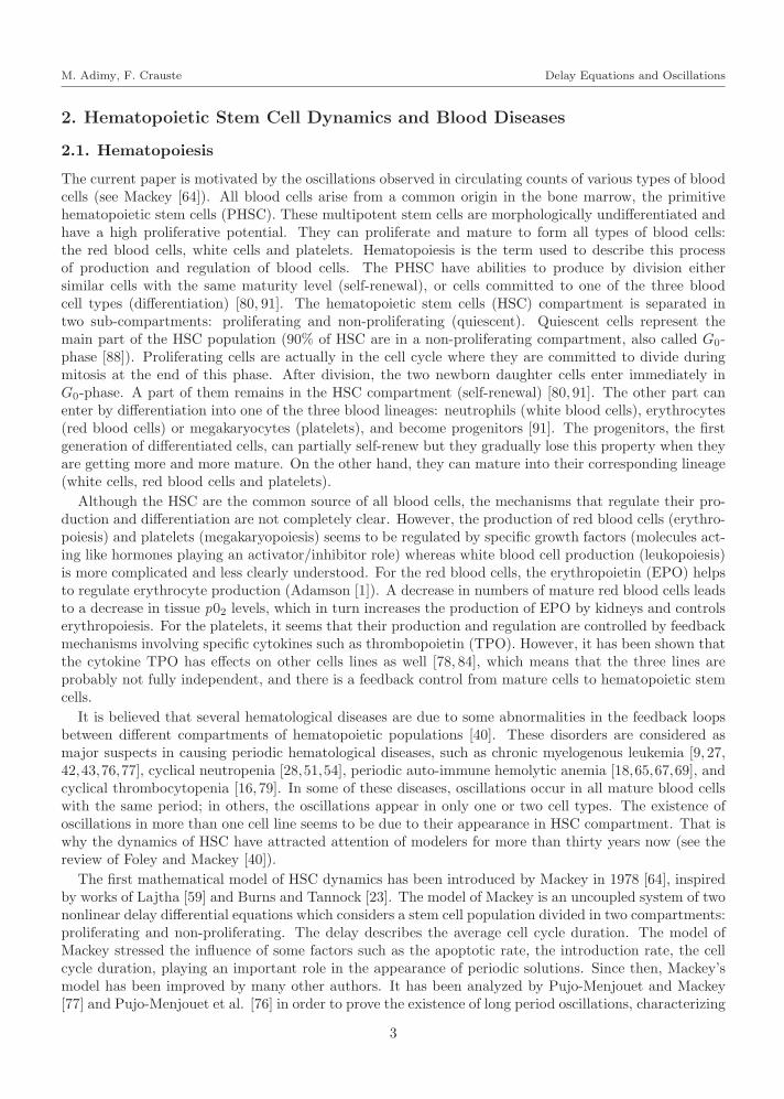
Equation (3.4) can then exhibit periodic solutions provided that a Hopf bifurcation occurs at thepositive steady state N∗. A usual situation corresponds to the existence of two critical values of thedelay τ , that is the function Z0 has two roots and Z1 has no root (see Figure 2). When τ increases andreaches the first root of Z0 then a Hopf bifurcation occurs (see Proposition 3.3): this critical value isτc = 2.475 days in Figure 2. Then periodic solutions are observed for τ > τc. In fact, Equation (3.4) hasperiodic solutions, with increasing periods, as long as τ does not reach the second root of Z0, τ = 3.22days (Figure 3). When τ keeps on increasing, it finally reaches τmax where a transcritical bifurcationoccurs, and the positive steady state no longer exists.

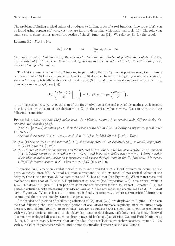
Amplitudes and periods of oscillating solutions of Equation (3.4) are displayed in Figure 3. One cansee that following the Hopf bifurcation periods of oscillations increase regularly, after an initial sharpincrease, from around 20 days up to 90 days. Mackey’s equation (3.4) is then able to exhibit oscillationswith very long periods compared to the delay (approximately 3 days), such long periods being observedin some hematological diseases such as chronic myeloid leukemia (see Section 2.2, and Pujo-Menjouet etal. [76]). It is noticeable, however, that amplitudes of the oscillations are rather constant, around 2− 2.5with our choice of parameter values, and do not specifically characterize the oscillations.

8


i

i

i

i

i

i

i


0 0.5 1 1.5 2 2.5 3−100

−90

−80

−70

−60

−50

−40

−30

−20

−10

0

10

τ (days)

Z k(τ)

Figure 2. Zk functions, k = 0 (top) and k = 1 (bottom). The function Z0 has tworoots, τ = 2.475 days at which a Hopf bifurcation occurs, and τ = 3.22 days. In thisillustration, τmax = 3.33 days, τ∗ = 3.25 days, and δ = 0.05 d−1, γ = 0.2 d−1, β0 = 1.77d−1, n = 3 and θ = 1 [31,76].

Stability of the positive steady state can also be investigated with respect to other parameters. Forinstance, let focus on the stability with respect to β∗. This choice will allow comparisons with a similarmodel exhibiting non-discrete delays in the next section. With β given by (3.3),

β∗ = β0θn θ

n − (n− 1)(N∗)n

(θn + (N∗)n)2.

Let consider β∗ = β∗(n). Fixing values of parameters δ, γ, β0 and θ (see Figure 2), and τ = 3 days, onecan see that there exists a critical value of β∗ (β∗

c = −0.33), or equivalently of n (nc = 2.33), for whichstability switch occurs through a Hopf bifurcation (see Figure 4). Contrary to the evolution observedwhen τ varies, in this case amplitudes and periods of the oscillations increase as −β∗ increases. For largevalues of n, −β∗ is larger and amplitudes of oscillations plateau. Larger observed periods of oscillationsare about 100 days, and the corresponding steady state value (not shown here) is close to, yet larger than,θ. Indeed, when n becomes large, the rate of introduction β is close to a threshold Heavyside function(see Pujo-Menjouet et al [76]), the threshold being equal to θ, and consequently N∗ approaches θ.

Several modifications of Mackey’s model have been proposed, accounting for different nonlinearities[31, 32] or more discrete delays [11, 27, 28] in order to describe the different hematopoietic lineages.Complexity increases in such models, yet they can roughly be analyzed in the same way. In the nextsection we consider a model for HSC dynamics with a distributed delay. The above-mentioned methodto determine the stability of the steady states and the existence of oscillations can not be applied todistributed delay.

9


i

i

i

i

i

i

i


2 2.5 3 3.50

10

20

30

40

50

60

70

80

90

100

τ (days)

Per

iod

(day

s)

2 2.5 3 3.50

0.5

1

1.5

2

2.5

3

Am

plitu

de

Figure 3. Amplitudes and periods of oscillating solutions of Equation (3.4). On theinterval [τ = 2.475, τ = 3.22], (3.4) has periodic solutions (parameter values are identicalto the ones used in Figure 2). Periods of the oscillations are displayed by the solid line,related to the left vertical axis, whereas amplitudes of oscillations are represented by thedashed line, and appear on the right vertical axis.

4. Model of HSC dynamics with Distributed Delay

Consider now Mackey’s model (Figure 1), with the same assumptions as in the previous section, exceptthat the length of the proliferating phase is assumed to be distributed according to a probability density— a probability kernel — denoted by f(a), with a ∈ (0, τ), where a denotes the time spent by a cellin the proliferating phase (its age) [2, 9, 33]. In the original Mackey’s model, presented in Section 3,the proliferating phase duration was supposed to be constant, the parameter τ representing an averageduration of this phase. This assumption however neglects variability of cell cycle durations. Hence,considering a non-constant distributed duration is a “natural” improvement of Mackey’s model.

Cell densities N(t) and P (t) now satisfy (Adimy et al. [9])

dN

dt(t) = −[δ + β(N(t))]N(t) + 2

∫ τ

0

e−γaf(a)β(N(t− a))N(t− a)da,

dP

dt(t) = −γP (t) + β(N(t))N(t)−

∫ τ

0

e−γaf(a)β(N(t− a))N(t− a)da,

(4.1)

with initial conditions defined for t ∈ [−τ, 0]. Previous assumptions on parameters δ and γ and functionβ still hold. In addition, we assume f is non-negative and satisfies

∫ τ

0

f(a)da = 1.

As previously noted, System (4.1) is not coupled, and the proliferating cell density P (t) can be expressedas

P (t) =

∫ τ

0

f(a)

(∫ t

t−a

e−γ(t−s)β(N(s))N(s) ds

)

da for t ≥ 0.

10


i

i

i

i

i

i

i


−0.5 0 0.5 1 1.5 2 2.5 3 3.50

10

20

30

40

50

60

70

80

90

100

−β*

Per

iod

(day

s)

−0.5 0 0.5 1 1.5 2 2.5 3 3.50

0.5

1

1.5

2

2.5

3

3.5

4

4.5

5

Am

plitu

de

Figure 4. Amplitudes and periods of oscillating solutions of Equation (3.4) as a functionof β∗. Equation (3.4) has periodic solutions for β∗ < β∗

c = −0.33 (Note that thehorizontal axis shows −β∗). Periods of the oscillations are displayed by the solid line,related to the left vertical axis, whereas amplitudes of oscillations are represented by thedashed line, and appear on the right vertical axis.

Hence we once again focus on the equation for N(t),

dN

dt(t) = −[δ + β(N(t))]N(t) + 2

∫ τ

0

e−γaf(a)β(N(t− a))N(t− a)da. (4.2)

Similarly to what we established in Proposition 3.1, we can state that Equation (4.2) has a unique positivesteady state N = N∗ provided that

(

2

∫ τ

0

e−γaf(a)da− 1

)

β(0) > δ, (4.3)

and it always has a trivial steady state N = 0. We determine the stability of the trivial steady state inthe following proposition.

Proposition 4.1. The trivial steady state N = 0 of Equation (4.2) is globally asymptotically stable if

(

2

∫ τ

0

e−γaf(a)da− 1

)

β(0) < δ, (4.4)

and unstable if (4.3) holds true.

Proof. Assume (4.4) holds, and denote by C+ the set of continuous nonnegative functions on [−τ, 0]. Letthe mapping J : C+ → [0,+∞) be defined by

J(ϕ) =

∫ ϕ(0)

0

β(s)s ds+

∫ τ

0

e−γaf(a)

(∫ 0

−a

(

β(

ϕ(θ))

ϕ(θ))2

dθ

)

da

11


i

i

i

i

i

i

i


for all ϕ ∈ C+. We set (see [49])

J(ϕ) = lim supt→0+

J(Nϕt )− J(ϕ)

t, for ϕ ∈ C+,

where Nϕ is the unique solution of (4.2) associated with the initial condition ϕ ∈ C+, and Nϕt (θ) =

Nϕ(t+ θ) for θ ∈ [−τ, 0]. Then, after computations (see [9]), one gets

J(ϕ) ≤ −

[

δ −

(

2

∫ τ

0

e−γaf(a)da− 1

)

β(ϕ(0))

]

β(ϕ(0))ϕ(0)2.

Since β is decreasing and nonnegative, and under assumption (4.4), the right hand side of the aboveinequality is negative for ϕ(0) ≥ 0, and vanishes if and only if ϕ(0) = 0. We deduce that every solutionof (4.2), with ϕ ∈ C+, tends to zero as t tends to +∞ [49].

Assume now (4.3) holds. The linearization of (4.2) around N ≡ 0 leads to the characteristic equation(see (4.6))

∆0(λ) := λ+ δ + β(0)− 2β(0)

∫ τ

0

e−(λ+γ)af(a)da = 0. (4.5)

Considering ∆0 as a real function, one can show (see [9]) that it has a unique real root, which is positive.Consequently, (4.5) has at least one characteristic root with positive real part, and the trivial steadystate is then unstable.

Condition (4.4) describes a situation in which the disappearance rate of non-proliferating cells is largerthan their proliferative rate, hence it characterizes a cell population inclined to extinction.

The local asymptotic stability analysis of the positive steady state N = N∗ can a priori be performedsimilarly to what has been presented in Section 3. Linearizing Equation (4.2) around N∗ leads to thecharacteristic equation

λ+ δ + β∗ − 2β∗

∫ τ

0

e−γaf(a)e−λada = 0, (4.6)

where β∗ := β(N∗) + N∗β′(N∗). The previous stability analysis, however, focused on the role of theparameter τ , the average proliferating phase duration, on the stability of the steady state. In the dis-tributed delay case, the duration of the proliferating phase is not characterized only by τ , the maximallength of the phase, but also by the probability density f(a). It is then not necessarily relevant to analyzethe stability with respect to τ . Indeed, any parameter can be used as a bifurcation parameter. We willchoose, in the following, β∗ as a bifurcation parameter.

It can nevertheless be noticed that stability can be analyzed when τ = 0. In this case, f(a) is a Diracmass in a = 0, and similarly to the result presented in Section 3 one can see that the positive steadystate is locally asymptotically stable since there is only one real eigenvalue, λ = β∗ − δ = N∗β′(N∗) < 0,with β(N∗) = δ.

When searching for a stability switch, it is not possible to reproduce the results of Section 3. Indeed,if one searches for purely imaginary roots λ = iω, with ω > 0, then separating real and imaginary partsin (4.6) leads to

C(ω) =δ + β∗

2β∗and S(ω) = −

ω

2β∗, (4.7)

where

C(ω) :=

∫ τ

0

e−γaf(a) cos(ωa)da and S(ω) :=

∫ τ

0

e−γaf(a) sin(ωa)da.

Summing up the squares of both sides of System (4.7) does not allow to isolate ω and express it as theroot of a polynomial function. Hence, an other approach must be used to investigate stability switch.

By investigating properties of the characteristic function in (4.6), we can then state the followingproposition, adapted from [9].

12


i

i

i

i

i

i

i


Proposition 4.2. Assume that (4.3) holds. If

β∗ ≥ −δ

2

∫ τ

0

e−γaf(a)da+ 1

, (4.8)

then the positive steady state N = N∗ of Equation (4.2) is locally asymptotically stable.

Proof. When β∗ ≥ 0, ∆(λ), given by (4.6), is shown to possess only one real root, λ0, negative, and allother characteristic roots λ of (4.6) satisfy Re(λ) < λ0. Consequently, N = N∗ is locally asymptoticallystable.

When β∗ < 0 and satisfies (4.8), one can show, by contradiction, that all eigenvalues have negativereal parts, implying that N∗ is also locally asymptotically stable.

Using the expression of β in (3.3), one can check that

β∗ = β0θn θ

n − (n− 1)(N∗)n

(θn + (N∗)n)2

and consequently β∗ does not have a constant sign. More precisely β∗ > 0 as long as N∗ < θ(1/(n −1))(1/n). This remark is also valid for the case with constant delay: indeed, the expression of β∗ is thesame as in the previous case, only the expression of the steady state value N∗ changes (see hereafter).Consequently, monotonicity properties of β∗ do not qualitatively change in the distributed delay case.

Moreover,

N∗ := β−1

δ

2

∫ τ

0

e−γaf(a)da− 1

,

where β−1 is a decreasing function mapping (0, β(0)] into [0,+∞). Therefore, N∗ approaches 0 whenInequality (4.3) is close to equality. This corresponds to a transcritical bifurcation: a stable positivesteady state disappears when an unstable trivial steady state switches stability and becomes stable.

When (4.8) does not hold (this implies in particular β∗ < 0), one can focus on the existence of a stabilityswitch and the occurrence of a bifurcation. Assume β∗ < κ, where κ := −δ/(2

∫ τ

0e−γaf(a)da + 1), and

search for purely imaginary roots of (4.6), λ = ±iω, with ω > 0. Then (ω, β∗) satisfies (4.7). Let usconsider the equation

g(ω) :=ω (1− 2C(ω))

2S(ω)= δ, ω > 0. (4.9)

Assume the function a 7→ e−γaf(a) is decreasing. From Lemma 4.1 and its proof, in [9], there exists asolution ωc > 0 of (4.9), which is not necessarily unique, and S(ωc) > 0. Since g(ωc) = δ > 0, then1− 2C(ωc) > 0. Using this critical value of ω, we can then define

β∗c := −

δ

1− 2C(ωc)< 0,

and straightforwardly check that β∗c < κ. Consequently, (ωc, β

∗c ) is a solution of (4.7), and ±iωc are

characteristic roots of (4.6) for β∗ = β∗c .

Denote by α the quantity

α :=

(

2

∫ τ

0

e−γaf(a)da− 1

)

β(0),

and define the sets

Ω := ω > 0; 0 < g(ω) < α and g′(ω) = 0 and Λ := g(Ω).

13


i

i

i

i

i

i

i


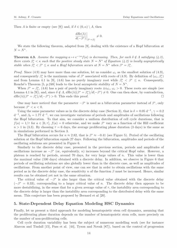
Then Λ is finite or empty (see [9]) and, if δ ∈ (0, α) \ Λ, then

dRe(λ)

d(−β∗)

∣

∣

∣

∣

β∗=β∗

c

6= 0.

We state the following theorem, adapted from [9], dealing with the existence of a Hopf bifurcation atN = N∗.

Theorem 4.3. Assume the mapping a 7→ e−γaf(a) is decreasing. Then, for each δ /∈ Λ satisfying (4.3),there exists β∗

c < κ such that the positive steady state N = N∗ of Equation (4.2) is locally asymptoticallystable when β∗

c < β∗ ≤ κ and a Hopf bifurcation occurs at N = N∗ when β∗ = β∗c .

Proof. Since (4.9) may have more than one solution, let us consider ωc as the smallest solution of (4.9),and consequently β∗

c is the maximum value of β∗ associated with roots of (4.9). By definition of (ωc, β∗c )

and from Lemma 4.1 in [9], (4.6) has no purely imaginary root while β∗c < β∗ ≤ κ. Consequently,

Rouche’s Theorem [5, p.248] leads to the local asymptotic stability of N = N∗.When β∗ = β∗

c , (4.6) has a pair of purely imaginary roots ±iωc, ωc > 0. These roots are simple (seeLemma 4.1 in [9]), and, since δ /∈ Λ, dRe(λ)(β∗ = β∗

c )/d(−β∗) 6= 0. One can then show, by contradiction,dRe(λ)(β∗ = β∗

c )/d(−β∗) > 0. This ends this proof.

One may have noticed that the parameter −β∗ is used as a bifurcation parameter instead of β∗, onlybecause β∗ < κ < 0.

Using the same parameter values as in the discrete delay case (Section 3), that is δ = 0.05 d−1, γ = 0.2d−1, and β0 = 1.77 d−1, we can investigate variations of periods and amplitudes of oscillations followingthe Hopf bifurcation. To that aim, we consider a uniform distribution of cell cycle durations, that isf(a) = 1/τ for a ∈ [0, τ ], f(a) = 0 otherwise, and we make β∗ vary as a function of the Hill coefficientn > 1 in (3.3). By choosing τ = 6 days, the average proliferating phase duration (3 days) is the same asin simulations performed in Section 3.

The Hopf bifurcation occurs for n ≈ 2.82, that is β∗ ≈ −0.41 (see Figure 5). Period of the oscillatingsolution at the Hopf bifurcation equals 27 days. Following the bifurcation, amplitudes and periods of theoscillating solutions are presented in Figure 6.

Similarly to the discrete delay case, presented in the previous section, periods and amplitudes ofoscillations increase as −β∗ (or, equivalently, n) increases beyond the critical Hopf value. However, aplateau is reached by periods, around 70 days, for very large values of n. This value is lower thanthe maximal value (100 days) obtained with a discrete delay. In addition, we observe in Figure 6 thatperiods of oscillating solutions are also globally lower than in the discrete case, as well as amplitudes ofoscillations. From another point of view, one can see that in order to obtain oscillations with the sameperiod as in the discrete delay case, the sensitivity n of the function β must be increased. Hence, similarresults can be obtained yet not in the same situation.

The critical value of −β∗ is also larger than the critical value obtained with the discrete delay(−β∗ = 0.33), corresponding to a larger critical value of n. The discrete delay then appears to bemore destabilizing, in the sense that for a given average value of τ , the instability area corresponding tothe discrete delay is larger than the instability area corresponding to the distributed delay with the samemean. This conjecture has been proposed by Bernard et al [20].

5. State-Dependent Delay Equation Modeling HSC Dynamics

Finally, let us present a third approach for modeling hematopoietic stem cell dynamics, assuming thatthe proliferating phase duration depends on the number of hematopoietic stem cells, more precisely onthe number of non-proliferating cells.

Cell cycle duration variability has been the subject of numerous modelling work (see for instanceAlarcon and Tindall [15], Fuss et al. [44], Tyson and Novak [87]), based on the control of progression

14


i

i

i

i

i

i

i


0 100 200 300 400 500 600 700 800 900 10001.4

1.5

1.6

1.7

1.8

1.9

2

2.1

Time (days)

Cel

l cou

nt N

(t)

Figure 5. Periodic solution of Equation (4.2) at the Hopf bifurcation. Parameter valuesare δ = 0.05 d−1, γ = 0.2 d−1, β0 = 1.77 d−1, θ = 1 , τ = 6 days and n = 2.82. Periodof the oscillations is around 27 days.

through the different phases of the cell cycle by protein concentration. In [15], the authors considerin particular the influence of extracellular factors (nutrients) in the regulation of cell cycle duration inbudding yeast. These nutrients are consumed by cells, and this triggers the progression through the cellcycle phases. Since proliferating cells are indeed cells committed to divide (once they have passed theG1/S transition), one can assume that they no longer consume nutrients. In addition, proliferating HSCrepresent only about 5% of all HSC [24], so their role in cell cycle regulation can be neglected and onecan consider that only non-proliferating cells control cell cycle durations.

This assumption leads to a modification of the initial Mackey’s model [64], which becomes a state-dependent delay system. Assume the cell cycle duration τ depends on the densityN(t) of non-proliferatingcells, and more particularly, that τ = µτ(N(t)), with µ ≥ 0. The function τ(N) is assumed to be bounded,positive, continuously differentiable and an increasing function of N , since it is a decreasing function ofthe quantity of available nutrients, which is a decreasing function of the number of non-proliferating cells.Let us define

τmin := infx≥0

τ(x) = τ(0) and τmax = supx≥0

τ(x).

All other assumptions and parameter notations are similar to the ones in Sections 3 and 4. FollowingAdimy et al [7], the cell density N(t) satisfies, for t ≥ 0,

N ′(t) = − [δ + β(N(t))]N(t) + 2e−γµτ(N(t))β(N(t− µτ(N(t))))N(t− µτ(N(t))), (5.1)

with an initial condition defined for t ∈ [−µτmax, 0]. Existence and uniqueness of solutions of (5.1) arenot straightforwardly obtained, yet this can be shown (see [7]) using Mallet-Paret et al. [68] and Walther[89]. Moreover, (5.1) has a trivial steady state, N = 0, and a positive steady state N = N∗ provided that

(2e−γµτmin − 1)β(0) > δ, or, equivalently, 0 ≤ µ <1

γτminln

(

2β(0)

β(0) + δ

)

:= µ. (5.2)

15


i

i

i

i

i

i

i


−0.5 0 0.5 1 1.5 2 2.5 3 3.50

10

20

30

40

50

60

−β*

Per

iod

(day

s)

−0.5 0 0.5 1 1.5 2 2.5 3 3.50

0.5

1

1.5

2

2.5

3

3.5

4

Am

plitu

de

Figure 6. Amplitudes and periods of oscillating solutions of Equation (4.2). For −β∗ <0.41 (equivalent to n < 2.82) the steady state N = N∗ is locally asymptotically stableand solutions converge towards N = N∗. For −β∗ > 0.41, (4.2) has periodic solutions.Periods of the oscillations are displayed by the solid line, related to the left vertical axis,whereas amplitudes of oscillations are represented by the dashed line, and appear on theright vertical axis. Parameter values are: δ = 0.05 d−1, γ = 0.2 d−1, β0 = 1.77 d−1,θ = 1, τ = 6 days.

The positive steady state value is then given by

(2e−γµτ(N∗) − 1)β(N∗) = δ, with µ ∈ [0, µ). (5.3)

One can notice that N∗ is not explicitly obtained, contrary to the previous discrete and continuousdistributed delay cases. However, using the Implicit Function Theorem, one can show that N∗ is adecreasing continuously differentiable function of µ [7].

We will show that Equation (5.1) can have oscillating solutions following a Hopf bifurcation at thepositive steady state, and we will use µ as the bifurcation parameter.

Linearization of (5.1) around N∗ leads to the characteristic exponential polynomial

∆(λ, µ) := λ+ δ + β∗(µ) + µτ ′(N∗(µ))α∗(µ)e−γµτ(N∗(µ)) − 2β∗(µ)e−γµτ(N∗(µ))e−λµτ(N∗(µ)),

where the dependence of the steady state value N∗ on µ is explicitly mentioned, and

α∗ (µ) = 2γβ(N∗ (µ))N∗ (µ) and β∗ (µ) = β(N∗ (µ)) + β′(N∗ (µ))N∗ (µ) .

One can show (see Adimy et al. [7], Theorem 6.1) that the positive steady state N = N∗ undergoes atranscritical bifurcation when µ = µ. Moreover, when µ = 0, N∗ is locally asymptotically stable, sincethe only characteristic root of ∆(λ, 0) is λ = β′(N∗(0))N∗(0) < 0. Hence, existence of stability switchesin the interval µ ∈ (0, µ) can be investigated.

Defining, for µ ∈ [0, µ),

b(µ) = δ + β∗(µ) + µτ ′(N∗(µ))α∗(µ)e−γµτ(N∗(µ)) and c(µ) = −2β∗(µ)e−γµτ(N∗(µ)),

16


i

i

i

i

i

i

i


the characteristic equation of (5.1) around N = N∗ can be written as

∆(λ, µ) := λ+ b(µ) + c(µ)e−λµτ(N∗(µ)) = 0. (5.4)

Let us search for purely imaginary roots of ∆(·, µ), denoted by λ = iω, with ω > 0 (one may note thatλ = 0 is not a characteristic root, and if iω is a characteristic root then so is −iω). Then (ω, µ) satisfies

ω = c(µ) sin(ωµτ (N∗(µ))),

b(µ) = −c(µ) cos(ωµτ (N∗(µ))).(5.5)

A necessary condition for equation (5.4) to have purely imaginary roots is

| c(µ) |>| b(µ) | . (5.6)

It is straightforward that b(µ) + c(µ) > 0. Then, for (5.6) to hold true, it is necessary that c(µ) > 0,that is β∗(µ) < 0. A sufficient condition for (5.6) is then b(µ) < 0, which is equivalent to

δ + β(N∗(µ)) + η(N∗(µ)) + 2γµσ(N∗(µ))β(N∗(µ))e−γµτ(N∗(µ)) < 0, (5.7)

where η : y ∈ [0,+∞) → η(y) = yβ′(y) ∈ (−∞, 0] and σ : y ∈ [0,+∞) → σ(y) = yτ ′(y) ∈ [0,+∞).Assuming η and σ are decreasing on the interval [0, β−1(δ)], and η

(

β−1(δ))

< −2δ, then there exists aunique µ∗ ∈ (0, µ) such that condition (5.7) is satisfied if and only if µ ∈ [0, µ∗) (see Adimy et al. [7]).

In the sequel, we assume there exists µ∗ ∈ (0, µ) such that (5.6) is fulfilled for µ ∈ [0, µ∗).

Adding the squares of both sides of (5.5), purely imaginary eigenvalues iω of (5.4), with ω > 0, mustsatisfy

ω =(

c2(µ)− b2(µ))

12 = ω(µ), µ ∈ [0, µ∗). (5.8)

Substituting expression (5.8) for ω in (5.5), we obtain

cos(

µτ∗(µ)(

c2(µ)− b2(µ))

12

)

= −b(µ)

c(µ),

sin(

µτ∗(µ)(

c2(µ)− b2(µ))

12

)

=

(

c2(µ)− b2(µ))

12

c(µ),

(5.9)

where τ∗ (µ) := τ (N∗(µ)).

From the above reasoning, values of µ ∈ [0, µ∗) solutions of system (5.9) generate positive ω(µ) givenby (5.8), and hence yield imaginary eigenvalues of (5.4). Consequently, we search for positive solutions µof (5.9) in the interval [0, µ∗). They satisfy

µτ∗(µ)(

c2(µ)− b2(µ))

12 = arccos

(

−b(µ)

c(µ)

)

+ 2kπ, k ∈ N0,

where N0 denotes the set of all nonnegative integers. Values of µ for which ω(µ) =(

c2(µ)− b2(µ))

12 is a

solution of (5.5) are roots of the functions

Zk(µ) = µ− µk(µ) :=arccos

(

− b(µ)c(µ)

)

+ 2kπ

τ∗(µ) (c2(µ)− b2(µ))12

, k ∈ N0, µ ∈ [0, µ∗). (5.10)

The next theorem states the existence of a Hopf bifurcation at N = N∗ for a critical value of theparameter µ (see Adimy et al. [7]).

17


i

i

i

i

i

i

i


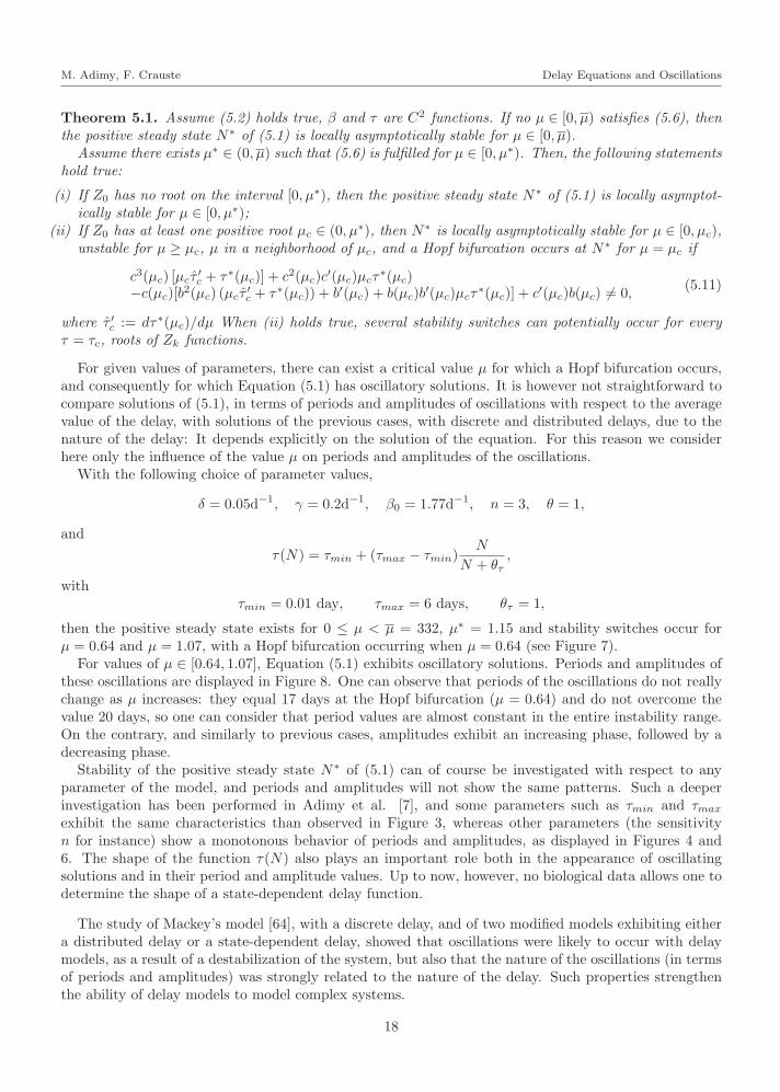
Theorem 5.1. Assume (5.2) holds true, β and τ are C2 functions. If no µ ∈ [0, µ) satisfies (5.6), thenthe positive steady state N∗ of (5.1) is locally asymptotically stable for µ ∈ [0, µ).

Assume there exists µ∗ ∈ (0, µ) such that (5.6) is fulfilled for µ ∈ [0, µ∗). Then, the following statementshold true:

(i) If Z0 has no root on the interval [0, µ∗), then the positive steady state N∗ of (5.1) is locally asymptot-ically stable for µ ∈ [0, µ∗);

(ii) If Z0 has at least one positive root µc ∈ (0, µ∗), then N∗ is locally asymptotically stable for µ ∈ [0, µc),unstable for µ ≥ µc, µ in a neighborhood of µc, and a Hopf bifurcation occurs at N∗ for µ = µc if

c3(µc) [µcτ′c + τ∗(µc)] + c2(µc)c

′(µc)µcτ∗(µc)

−c(µc)[b2(µc) (µcτ

′c + τ∗(µc)) + b′(µc) + b(µc)b

′(µc)µcτ∗(µc)] + c′(µc)b(µc) 6= 0,

(5.11)

where τ ′c := dτ∗(µc)/dµ When (ii) holds true, several stability switches can potentially occur for everyτ = τc, roots of Zk functions.

For given values of parameters, there can exist a critical value µ for which a Hopf bifurcation occurs,and consequently for which Equation (5.1) has oscillatory solutions. It is however not straightforward tocompare solutions of (5.1), in terms of periods and amplitudes of oscillations with respect to the averagevalue of the delay, with solutions of the previous cases, with discrete and distributed delays, due to thenature of the delay: It depends explicitly on the solution of the equation. For this reason we considerhere only the influence of the value µ on periods and amplitudes of the oscillations.

With the following choice of parameter values,

δ = 0.05d−1, γ = 0.2d−1, β0 = 1.77d−1, n = 3, θ = 1,

and

τ(N) = τmin + (τmax − τmin)N

N + θτ,

withτmin = 0.01 day, τmax = 6 days, θτ = 1,

then the positive steady state exists for 0 ≤ µ < µ = 332, µ∗ = 1.15 and stability switches occur forµ = 0.64 and µ = 1.07, with a Hopf bifurcation occurring when µ = 0.64 (see Figure 7).

For values of µ ∈ [0.64, 1.07], Equation (5.1) exhibits oscillatory solutions. Periods and amplitudes ofthese oscillations are displayed in Figure 8. One can observe that periods of the oscillations do not reallychange as µ increases: they equal 17 days at the Hopf bifurcation (µ = 0.64) and do not overcome thevalue 20 days, so one can consider that period values are almost constant in the entire instability range.On the contrary, and similarly to previous cases, amplitudes exhibit an increasing phase, followed by adecreasing phase.

Stability of the positive steady state N∗ of (5.1) can of course be investigated with respect to anyparameter of the model, and periods and amplitudes will not show the same patterns. Such a deeperinvestigation has been performed in Adimy et al. [7], and some parameters such as τmin and τmax

exhibit the same characteristics than observed in Figure 3, whereas other parameters (the sensitivityn for instance) show a monotonous behavior of periods and amplitudes, as displayed in Figures 4 and6. The shape of the function τ(N) also plays an important role both in the appearance of oscillatingsolutions and in their period and amplitude values. Up to now, however, no biological data allows one todetermine the shape of a state-dependent delay function.

The study of Mackey’s model [64], with a discrete delay, and of two modified models exhibiting eithera distributed delay or a state-dependent delay, showed that oscillations were likely to occur with delaymodels, as a result of a destabilization of the system, but also that the nature of the oscillations (in termsof periods and amplitudes) was strongly related to the nature of the delay. Such properties strengthenthe ability of delay models to model complex systems.

18

“mmnp˙Adimy-Crauste” — 2012/12/4 — 10:23 — page 19 — #19

i

i

i

i

i

i

i

i


0 0.2 0.4 0.6 0.8 1−10

−8

−6

−4

−2

0

2

µ

Z k(µ),

(k=0

, k=1

)

Figure 7. Zk(µ) functions, for µ ∈ [0, µ∗), with µ∗ = 1.15. The top curve is Z0(µ),it exhibits two roots, for µ = 0.64 and µ = 1.07, and the bottom curve is Z1(µ), it isstrictly negative. Parameter values are: δ = 0.05 d−1, γ = 0.2 d−1, β0 = 1.77 d−1, θ = 1,n = 3, τmin = 0.01 days, τmax = 6 days, and θτ = 1.

Acknowledgements. The work of FC has been supported by the ANR grant ProCell ANR-09-JCJC-0100-01.

References

[1] J.W. Adamson. Regulation of red blood cell Production. Am. J. Med., 101 (1996), S4–S6.

[2] M. Adimy, F. Crauste. Global stability of a partial differential equation with distributed delay due to cellular replication.Nonlinear Analysis, 54 (2003), 1469–1491.

[3] M. Adimy, F. Crauste. Modelling and asymptotic stability of a growth factor-dependent stem cells dynamics modelwith distributed delay. Discrete and Continuous Dynamical Systems Series B, 8 (2007), No. 1, 19–38.

[4] M. Adimy, F. Crauste. Mathematical model of hematopoiesis dynamics with growth factor-dependent apoptosis andproliferation regulation. Mathematical and Computer Modelling, 49 (2009), 2128–2137.

[5] M. Adimy, F. Crauste, A. El Abdllaoui. Asymptotic Behavior of a Discrete Maturity Structured System of Hematopoi-etic Stem Cells Dynamics with Several Delays. Mathematical Modelling of Natural Phenomena, Vol 1 (2006), No. 2,1–22.

[6] M. Adimy, F. Crauste, A. El Abdllaoui. Discrete maturity-structured model of cell differentiation with applications toacute myelogenous leukemia. J. Biol. Syst., 16 (3) (2008), 395–424.

[7] M. Adimy, F. Crauste, M.L. Hbid, R. Qesmi. Stability and Hopf bifurcation for a cell population model with state-dependent delay. SIAM J. Appl. Math, 70 (5) (2010), 1611–1633.

[8] M. Adimy, F. Crauste, C. Marquet. Asymptotic behavior and stability switch for a mature-immature model of celldifferentiation. Nonlinear Analysis: Real World Applications, 11 (2010), 2913–2929.

[9] M. Adimy, F. Crauste, S. Ruan. A mathematical study of the hematopoiesis process with applications to chronicmyelogenous leukemia. SIAM J. Appl. Math., 65 (2005), 1328–1352.

[10] M. Adimy, F. Crauste, S. Ruan. Stability and Hopf bifurcation in a mathematical model of pluripotent stem celldynamics. Nonlinear Analysis: Real World Applications, 6 (2005), No. 4, 651–670.

[11] M. Adimy, F. Crauste, S. Ruan. Periodic Oscillations in Leukopoiesis Models with Two Delays. J. Theo. Biol., 242(2006), 288–299.

[12] M. Adimy, F. Crauste, S. Ruan. Modelling hematopoiesis mediated by growth factors with applications to periodichematological diseases. Bulletin of Mathematical Biology, 68 (8) (2006), 2321–2351.

19


i

i

i

i

i

i

i

i


0.65 0.7 0.75 0.8 0.85 0.9 0.95 1 1.05 1.10

5

10

15

20

25

µ

Per

iod

(day

s)

0.65 0.7 0.75 0.8 0.85 0.9 0.95 1 1.05 1.10

0.5

1

1.5

2

2.5

Am

plitu

de

Figure 8. Amplitudes and periods of oscillating solutions of Equation (5.1). For µ <0.64, the positive steady state is locally asymptotically stable and solutions convergetowards N∗. The same holds for µ > 1.07. In between, oscillatory solutions are observed,with periods of the oscillations displayed by the solid line, related to the left vertical axis,and amplitudes represented by the dashed line, values appearing on the right verticalaxis. Parameter values are: δ = 0.05 d−1, γ = 0.2 d−1, β0 = 1.77 d−1, θ = 1, n = 3,τmin = 0.01 days, τmax = 6 days, and θτ = 1.

[13] W. Aiello, H. Freedman, J. Wu. Analysis of a model representing stage-structured population growth with stage-dependent time delay. SIAM Journal of Applied Mathematics 52 (1992), 855–869.

[14] U. an der Heiden. Delays in physiological systems. J. Math. Biol. 8 (1979), 345–364.

[15] T. Alarcon, M.J. Tindall. Modelling Cell Growth and its Modulation of the G1/S Transition. Bull. Math. Biol., 69(2007), 197–214.

[16] R. Apostu, M.C. Mackey. Understanding cyclical thrombocytopenia: a mathematical modeling approach. J. Theor.Biol., 251 (2008), 297–316.

[17] J.J. Batzel, F. Kappel. Time delay in physiological systems: Analyzing and modeling its impact. Math. Biosciences,234 (2011), No. 2, 61–74.

[18] J. Belair, M.C. Mackey, J.M. Mahaffy. Age-structured and two-delay models for erythropoiesis. Math. Biosci., 128(1995), 317–346.

[19] E. Beretta, Y. Kuang. Geometric stability switch criteria in delay differential systems with delay dependent parameters.SIAM J. Math. Anal., 33 (2002), No. 5, 1144–1165.

[20] S. Bernard, J. Belair, M.C. Mackey. Sufficient conditions for stability of linear differential equations with distributeddelay. Discrete Contin. Dyn. Syst. Ser. B., 1 (2001), 233–256.

[21] S. Bernard, J. Belair, M.C. Mackey. Oscillations in cyclical neutropenia: new evidence based on mathematical modeling.J. Theor. Biol., 223 (2003), 283–298.

[22] M. Bodnar, A. Bart lomiejczyk. Stability of delay induced oscillations in gene expression of Hes1 protein model. Non-linear Analysis: Real World Applications, 13 (2012), 2227–2239.

[23] F.J. Burns, I.F. Tannock. On the existence of a G0 phase in the cell cycle. Cell Tissue Kinet., 19 (1970), 321–334.

[24] S.H. Cheshier, S. J. Morrison, X. Liao, I.L. Weissman. In vivo proliferation and cell cycle kinetics of long-term self-renewing hematopoietic stem cells. Proc. Natl. Acad. Sci. USA, 96 (1999), 3120–3125.

[25] M.S. Ciupe, B.L. Bivort, D.M. Bortz, P.W. Nelson. Estimating kinetic parameters from HIV primary infection datathrough the eyes of three different mathematical models. Math Biosci. 200(1) 2006, 1–27.

20


i

i

i

i

i

i

i

i


[26] C. Colijn, C. Foley, M.C. Mackey. G-CSF treatment of canine cyclical neutropenia: A comprehensive mathematicalmodel. Exper. Hematol. (2007), 35, 898–907.

[27] C. Colijn, M.C. Mackey. A mathematical model of hematopoiesis – I. Periodic chronic myelogenous leukemia. J. Theor.Biol., 237 (2005), 117–132.

[28] C. Colijn, M.C. Mackey. A mathematical model of hematopoiesis – II. Cyclical neutropenia. J. Theor. Biol., 237 (2005),133–146.

[29] L. Cooke. Stability analysis for a vector disease model. Rocky Mountain J. Math., 9 (1979), 31–42.

[30] A.S. Coutts, C.J. Adams, N.B. La Thangue. p53 ubiquitination by Mdm2: a never ending tail? DNA Repair (Amst).8 (2009), 483–90.

[31] F. Crauste. Global Asymptotic Stability and Hopf Bifurcation for a Blood Cell Production Model. Math. Bio. Eng., 3(2006), No. 2, 325–346.

[32] F. Crauste. Delay Model of Hematopoietic Stem Cell Dynamics: Asymptotic Stability and Stability Switch. Mathe-matical Modeling of Natural Phenomena, 4 (2009), No. 2, 28–47.

[33] F. Crauste. Stability and Hopf bifurcation for a first-order linear delay differential equation with distributed delay, inComplex Time Delay Systems (Ed. F. Atay), Springer, 1st edition, 320 p., ISBN: 978-3-642-02328-6 (2010).

[34] L.A. Crews, C.H. Jamieson. Chronic myeloid leukemia stem cell biology. Curr Hematol Malig Rep., 7 (2012), No. 2,125–132.

[35] J.M. Cushing. Integrodifferential Equations and Delay Models in Population Dynamics. Springer-Verlag, Heidelberg,1977.

[36] D.C. Dale, A.A. Bolyard, A. Aprikyan. Cyclic neutropenia. Semin. Hematol., 39 (2002), 89–94.

[37] D.C. Dale, W.P. Hammond. Cyclic neutropenia: A clinical review. Blood Rev., 2 (1998), 178–185.

[38] J. Dieudonne. Foundations of Modern Analysis. Academic Press, New-York, 1960.

[39] C. Foley, S. Bernard, M.C. Mackey. Cost-effective G-CSF therapy strategies for cyclical neutropenia: Mathematicalmodelling based hypotheses. J. Theor. Biol. (2006), 238, 754–763.

[40] C. Foley, M.C. Mackey. Dynamic hematological disease: a review. J. Math. Biol., 58 (2009), 285–322.

[41] A.C. Fowler, M.J. McGuinness. A delay recruitment model of the cardiovascular control system. J. Math. Biol. 51(2005), 508–526.

[42] P. Fortin, M.C. Mackey. Periodic chronic myelogenous leukaemia: spectral analysis of blood cell counts and a etiologicalimplications. Br. J. Haematol., 104 (1999), 336–345.

[43] A. Fowler, M.C. Mackey. Relaxation oscillations in a class of delay differential equations. SIAM J. Appl. Math., 63(2002), 299–323.

[44] H. Fuss, W. Dubitzky, S. Downes, M.J. Kurth. Mathematical models of cell cycle regulation. Brief Bioinform., 6 (2005),163–177.

[45] N. Geva-Zatorsky , N. Rosenfeld, S. Itzkovitz, R. Milo, A. Sigal, E. Dekel, T. Yarnitzky, Y. Liron, P. Polak, G. Lahav,U. Alon. Oscillations and variability in the p53 system. Mol Syst Biol (2006), 2.2006.0033.

[46] K. Gopalsamy. Stability and Oscillations in Delay Differential Equations of Population. Dynamics, Kluwer Academic,Dordrecht, 1992.

[47] L. Glass, A. Beuter, D. Larocque. Time delays, oscillations, and chaos in physiological control systems. MathematicalBiosciences, 90 (1988), 111–125.

[48] D. Guerry, D. Dale, D.C. Omine, S. Perry, S.M. Wolff. Periodic hematopoiesis in human cyclic neutropenia. J ClinInvest. 52 (1973), 3220–3230.

[49] J. Hale, S.M. Verduyn Lunel. Introduction to functional differential equations. Applied Mathematical Sciences 99.Springer-Verlag, New York, 1993.

[50] Y. Haupt, R. Maya, A. Kazaz, M. Oren. Mdm2 promotes the rapid degradation of p53. Nature 387 (1997), 296–299.

[51] C. Haurie, D.C. Dale, M.C. Mackey. Cyclical neutropenia and other periodic hematological disorders: A review ofmechanisms and mathematical models. Blood, 92 (1998), 2629–2640.

[52] C. Haurie, D.C. Dale, M.C. Mackey. Occurrence of periodic oscillations in the differential blood counts of congenital,idiopathic, and cyclical neutropenic patient before and during treatment with G-CSF. Exp. Hematol., 27 (1999), 401–409.

[53] C. Haurie, D.C. Dale, R. Rudnicki, M.C Mackey. Modeling complex neutrophil dynamics in the grey collie. J TheorBiol. 204 (2000), 505–519.

[54] C. Haurie, R. Person, D.C. Dale, M.C. Mackey. Hematopoietic dynamics in grey collies. Exp. Hematol., 27 (1999),1139–1148.

[55] N.D. Hayes. Roots of the transcendental equation associated with a certain difference-differential equation. J. LondonMath. Soc., 25 (1950), 226–232.

[56] T. Hearn, C. Haurie, M.C. Mackey. Cyclical neutropenia and the peripheral control of white blood cell production. J.Theor. Biol. 192 (1998), 167–181.

[57] H. Hirata, S. Yoshiura, T. Ohtsuka, Y. Bessho, T. Harada, K. Yoshikawa, R. Kageyama. Oscillatory Expression of thebHLH Factor Hes1 Regulated by a Negative Feedback Loop. Science 298 (2002), 840–843.

[58] Y. Kuang. Delay Differential Equations with Applications in Population Dynamics. Academic Press, INC., San Diego,CA (1993).

[59] L.G. Lajtha. On DNA labeling in the study of the dynamics of bone marrow cell populations, in: Stohlman, Jr., F.(Ed), The Kinetics of Cellular Proliferation, Grune and Stratton, New York (1959), 173–182.

21


i

i

i

i

i

i

i


[60] J. Lei, M.C. Mackey. Multistability in an age-structured model of hematopoiesis: Cyclical neutropenia. J. Theor. Biol.,270 (2011), 143–153.

[61] J. Li, Y. Kuang, C. Mason. Modeling the glucose-insulin regulatory system and ultradian insulin secretory oscillationswith two time delays. J. Theoret. Biol., 242 (2006), 722–735.

[62] G.S. Longobardo, N.S. Cherniack, A.P. Fishman. Cheyne–Stokes breathing produced by a model of the human respira-tory system. J. Appl. Physiol. 21 (1966), 1839–1846.

[63] N. MacDonald. Time Lags in Biological Models. Springer-Verlag, Heidelberg, 1978.

[64] M.C. Mackey. Unified hypothesis of the origin of aplastic anaemia and periodic hematopoiesis. Blood, 51 (1978),941–956.

[65] M.C. Mackey. Periodic auto- immune hemolytic anemia: an induced dynamical disease. Bull. Math. Biol., 41 (1979),829–834.

[66] M.C. Mackey. Cell kinetic status of haematopoietic stem cells. Cell Prolif., 34 (2001), 71–83.

[67] J.M. Mahaffy, J. Belair, M.C. Mackey. Hematopoietic model with moving boundary condition and state dependantdelay. J. Theor. Biol., 190 (1998), 135–146.

[68] J. Mallet-Paret, R.D. Nussbaum, P. Paraskevopoulos. Periodic solutions for functional differential equations withmultiple state-dependent time lags. Topol. Methods Nonlinear Anal., 3 (1994), 101–162.

[69] J.G. Milton, M.C. Mackey. Periodic haematological diseases: mystical entities of dynamical disorders? J.R. Coll.Phys., 23 (1989), 236–241.

[70] N.A.M. Monk. Oscillatory expression of Hes1, p53, and NF-k B driven by transcriptional time delays. Curr. Biol. 13(2003), 1409–1413.

[71] A. Morley. Periodic diseases, physiological rhythms and feedback control-a hypothesis. Aust. Ann. Med. 3 (1970),244–249.

[72] A. Morley, A.G. Baikie, D.A.G. Galton. Cyclic leukocytosis as evidence for retention of normal homeostatic control inchronic granulocytic leukaemia. Lancet, 2 (1967), 1320–1322.

[73] A. Morley, E.A. King-Smith, F. Stohlman. The oscillatory nature of hemopoiesis. In: Stohlman, F. (Ed.), HemopoieticCellular Proliferation. Grune & Stratton, New York, (1969), 3–14.

[74] P.W. Nelson, J.D. Murray, A.S. Perelson. A model of HIV-1 pathogenesis that includes an intracellular delay. Math.Biosci., 163 (2000), 201–215.

[75] N. Pørksen, M. Hollingdal, C. Juhl, P. Butler, J. D. Veldhuis, O. Schmitz. Pulsatile insulin secretion: Detection,regulation, and role in diabetes. Diabetes, 51 (2002), S245–S254.

[76] L. Pujo-Menjouet, S. Bernard, M.C. Mackey. Long period oscillations in a G0 model of hematopoietic stem cells. SIAMJ. Appl. Dyn. Systems, 4 (2005), No. 2, 312–332.

[77] L. Pujo-Menjouet, M.C. Mackey. Contribution to the study of periodic chronic myelogenous leukemia. Comptes RendusBiologies, 327 (2004), 235–244.

[78] M.Z. Ratajczak, J. Ratajczak, W. Marlicz, et al. Recombinant human thrombopoietin (TPO) stimulates erythropoiesisby inhibiting erythroid progenitor cell apoptosis. Br J. Haematol., 98 (1997), 8–17.

[79] M. Santillan, J. Belair, J.M. Mahaffy, M.C. Mackey. Regulation of platelet production: The normal response to per-turbation and cyclical platelet disease. J. Theor. Biol., 206 (2000), 585–603.

[80] B.R. Smith. Regulation of hematopoiesis. Yale J Biol Med., 63 (1990), No. 5, 371–380.

[81] H.L. Smith. Reduction of structured population models to threshold-type delay equations and functional differentialequations: a case study. Math. Biosc., 113 (1993), 1–23.

[82] J. Sturis, K. S. Polonsky, E. Mosekilde, E. Van Cauter. Computer model for mechanisms underlying ultradian oscilla-tions of insulin and glucose. Am. J. Physiol., 260 (1991), E801–E809.

[83] M. Sturrock, A.J. Terry, D.P. Xirodimas, A.M. Thompson, M.A.J. Chaplain. Spatio-temporal modelling of the Hes1and p53-Mdm2 intracellular signalling pathways. J. Theor. Biol., 273 (2011), 15–31.

[84] S. Tanimukai, T. Kimura, H. Sakabe et al. Recombinant human c-Mpl ligand (thrombopoietin) not only acts onmegakaryocyte progenitors, but also on erythroid and multipotential progenitors in vitro. Experimental Hematology,25 (1997), 1025–1033.

[85] E. Terry, J. Marvel, C. Arpin, O. Gandrillon, F. Crauste. Mathematical Model of the primary CD8 T Cell ImmuneResponse: Stability Analysis of a Nonlinear Age-Structured System. J. Math. Biol. (to appear).

[86] I.M. Tolic, E. Mosekilde, J. Sturis. Modeling the insulin-glucose feedback system: The significance of pulsatile insulinsecretion. J. Theoret. Biol., 207 (2000), 361–375.

[87] J.J. Tyson, B. Novak. Regulation of the Eukaryotic Cell Cycle: Molecular Antagonism, Hysteresis, and IrreversibleTransitions. J. theor. Biol., 210 (2001), pp. 249–263.

[88] W. Vainchenker. Hematopoıese et facteurs de croissance. Encycl. Med. Chir., Hematologie, 13000 (1991), M85.

[89] H.O. Walther. The solution manifold and C1-smoothness of solution operators for differential equations with statedependent delay. J. Differential Eqs., 195 (2003), 46–65.

[90] G.F. Webb. Theory of Nonlinear Age-Dependent Population Dynamics. Monographs and textbook in Pure Appl.Math., 89, Marcel Dekker, New York (1985).

[91] I.L. Weissman. Stem cells: units of development, units of regeneration, and units in evolution. Cell, 100 (2002),157–168.

22

Documents

Delay Differential Equations and Autonomous Oscillations ...€¦ · The mechanism of the regulation of the Hes1 protein involves a negative feedback loop with one acti- ... (leukopoiesis)