Deliverable!D2.1! Progress!and!Activity!Report!onWP2!

FP7-‐ICT-‐2011.8 Contract no.: 318493

www.toposys.org

Deliverable D2.1

Progress and Activity Report on WP2

Deliverable Nature: Report (R)

Dissemination Level: (Confidentiality)

Public (PU)

Contractual Delivery Date: M12

Actual Delivery Date: M12

Version: 1.0

TOPOSYS Deliverable 2.1

Contents

1 Summary 2

2 Topology of Noise 32.1 Crackle . . . . . . . . . . . . . . . . . . . . . . . . . . . . . . . . . . . . . . . . . . . 3

2.1.1 Some sample results . . . . . . . . . . . . . . . . . . . . . . . . . . . . . . . . 52.1.2 Poisson Processes . . . . . . . . . . . . . . . . . . . . . . . . . . . . . . . . . . 72.1.3 Results . . . . . . . . . . . . . . . . . . . . . . . . . . . . . . . . . . . . . . . 7

2.2 Stationary Point Processes . . . . . . . . . . . . . . . . . . . . . . . . . . . . . . . . . 112.2.1 Some notation . . . . . . . . . . . . . . . . . . . . . . . . . . . . . . . . . . . 122.2.2 A result sampler . . . . . . . . . . . . . . . . . . . . . . . . . . . . . . . . . . 122.2.3 Some implications for topological data analysis . . . . . . . . . . . . . . . . . 142.2.4 Subgraph and component counts in random geometric graphs . . . . . . . . . 152.2.5 Some notation and a start . . . . . . . . . . . . . . . . . . . . . . . . . . . . . 152.2.6 Sparse regime: rn Ñ 0 . . . . . . . . . . . . . . . . . . . . . . . . . . . . . . . 172.2.7 Thermodynamic regime: rdn Ñ β . . . . . . . . . . . . . . . . . . . . . . . . . 182.2.8 Variance bounds for the sparse and thermodynamic regimes . . . . . . . . . . 192.2.9 Phase transitions in the sparse and thermodynamic regimes . . . . . . . . . . 202.2.10 Betti numbers of random geometric complexes . . . . . . . . . . . . . . . . . 202.2.11 Topological preliminaries . . . . . . . . . . . . . . . . . . . . . . . . . . . . . 212.2.12 Expectations of Betti numbers . . . . . . . . . . . . . . . . . . . . . . . . . . 222.2.13 Thresholds for homology groups . . . . . . . . . . . . . . . . . . . . . . . . . 232.2.14 Further results for the Ginibre process: . . . . . . . . . . . . . . . . . . . . . 242.2.15 Morse theory for random geometric complexes . . . . . . . . . . . . . . . . . 242.2.16 Morse Theory . . . . . . . . . . . . . . . . . . . . . . . . . . . . . . . . . . . . 252.2.17 Limit theorems for expected numbers of critical points . . . . . . . . . . . . . 26

3 Bayesian Persistence 283.1 Topological Features . . . . . . . . . . . . . . . . . . . . . . . . . . . . . . . . . . . . 283.2 Model Selection . . . . . . . . . . . . . . . . . . . . . . . . . . . . . . . . . . . . . . . 28

4 Smoothing 294.1 Gaussian Kernels . . . . . . . . . . . . . . . . . . . . . . . . . . . . . . . . . . . . . . 294.2 Harmonic Forms . . . . . . . . . . . . . . . . . . . . . . . . . . . . . . . . . . . . . . 29

1 Summary

Statistics is at the heart of data analysis - our main goal in this work package is to bring the strengthof statistics to topological tools. Our first task is to gain a better understanding of topologicalnoise. Most results in applied topology for approximating the underlying persistence or homologyof a space are of the form, given a sufficient sample, there exists some finite simplicial complex wecan build on top of our sample such that the answer we obtain will be correct or approximatelycorrect in the appropriate sense.

In particular for persistence, stability gives an upper bound on the magnitude of the noise.Importantly however, these are only upper bounds often in a form which are unsuitable for statisitcal

2


tests. Little is known how the “topological noise” behaves. This is important for constructing anull hypothesis as well as constructing algorithms which deal with outliers in a more robust waythan current topological methods.

In the first year, the concentration was on understanding the topology of noise better. Wepresent two results - this report is based on the following two papers:

1. “Crackle: The Persistent Homology of Noise,” R.J. Adler, O.Bobrowski, S. Weinberger (at-tached to this report and available at http://arxiv.org/pdf/1301.1466)

2. “On the topology of random complexes built over stationary point process’,’ D. Yogeshwaranand R.J. Adler, (attached to this report and available at http://arxiv.org/abs/1211.0061).

The text is in this report is based upon these papers - with proofs omitted here to highlight theresults. For any clarification please refer to the papers. An outline of the results is as follows:

1. Crackle - In most topological work, the noise is considered to eb absolutely bounded. However,a more common model in statistics is Gaussian noise and in complex systems heavier tails. Theresults show that in the presence of Gaussian noise, the outliers may be controlled relativelyeasily, while in the heavy tailed case (i.e. polynomial and certain exponential decays), maygive rise to crackle. That is we no longer have simply outliers, but topological structures(non-trivial homology classes) in all dimensions up to the ambient dimension. This highlightsthe importance of recognizing heavy tailed noise and mitigating it.

2. The second result extends work on i.i.d Poisson processes to stationary point processes, ob-taining asymptotic results in different regimes for the Betti numbers in expectation along withadditional characterizations.

In this work package we have two other tasks. They are still in a very preliminary phase and inthis document we only describe the initial planning and possible approaches for the coming year ofthe project.

2 Topology of Noise

2.1 Crackle

Here we look at the homology of simplicial complexes built via deterministic rules from a randomset of vertices. Depending on the randomness that generates the vertices, the homology of thesecomplexes can either become trivial as the sample size grows, or can contain more and more complexstructures.

The motivation for these results comes from applications of topological tools for pattern analysis,object identification, and especially for the analysis of data sets. Typically, one starts with acollection of points and forms some simplicial complexes associated to these, and then takes theirhomology. For example, the 0-dimensional homology of such complexes can be interpreted as aversion of clustering. The basic philosophy behind this attempt is that topology has an essentiallyqualitative nature and should therefore be robust with respect to small perturbations. Some recentreferences are [2, 3, 11, 22, 29] with two reviews, from different aspects, in [1] and [17]. Many ofthese papers find their raison d’etre in essentially statistical problems, in which data generates thestructures.

3

http://arxiv.org/pdf/1301.1466

http://arxiv.org/abs/1211.0061


An important example occurs in the following manifold learning problem. LetM be an unknownmanifold embedded in a Euclidean space, and suppose that we are a given a set of independent andidentically distributed (i.i.d.) random samples Xn “ tX1, . . . , Xnu from the manifold. In order torecover the homology of M, we consider the homology of

U “

nď

k“1

BεpXkq, (2.1)

where BεpXq is the Euclidean ball, in the ambient space, of radius ε about the point X. Thebelief, or hope, is that, for large enough n, the homology of U will be equivalent to that of M. Aconfounding issue arises when the sample points do not necessarily lie on the manifold, but ratherare perturbed from it by a random amount. When this happens, it will follow from our results thatthe precise distribution behind the randomness plays a qualitatively important role. It is knownthat if the perturbations come from a bounded or strongly concentrated distribution, then they donot lead to much spurious homology, and the above line of attack, appropriately applied, works.For example, it was shown in [26] that for Gaussian noise it is possible to clean the data and recoverthe underlying topology of M in a way that is essentially independent on the ambient dimension.Both [25, 26] contain results of the form that, given a nice enough M, and any δ ą 0, there areexplicit conditions on n and ε such that the homology of U is equal to the homology of M with aprobability of at least p1 ´ δq. However, for other distributions no such results exist, nor, in viewof the results of this paper, are they to be expected.

Figure 1 provides an illustrative example of what happens when sampling points from an an-nulus and perturbing them with additional noise before reconstructing the annulus as in (2.1). Inparticular, it shows that if the additional noise is in some sense large then sample points can appearbasically anywhere, introducing extraneous homology elements.

(a) (b) (c) (d)

Figure 1: (a) The original space M (an annulus) that we wish to recover from random samples.(b) With the appropriate choice of radius, we can easily recover the homology of the originalspace from random samples from M. (c) In the presence of bounded noise, homology recovery isundamaged. (d) In the presence of unbounded noise, many extraneous homology elements appear,and significantly interfere with homology recovery.

In order to be able, eventually, to extend the work in [26] beyond Gaussian noise, and make moreconcrete statements about the probabilistic features of the homology this extension generates, it isnecessary to first focus on the behaviour of samples generated by pure noise, with no underlyingmanifold. In this case, thinking of the above setup, the manifold M is simply the point at theorigin, and the homology that we shall be trying to recapture is trivial. Nevertheless, we shall seethat differing noise models can make this task extremely delicate, regardless of sample size.

4


2.1.1 Some sample results

To start being more concrete, letXn “ tX1, . . . , Xnu

be a set of n i.i.d. random samples in Rd, from a common density function f . Recall that theabstract simplicial complex CpX , εq constructed according to the following rules is called the Cechcomplex associated to X and ε:

1. The 0-simplices of CpX , εq are the points in X ,

2. An n-simplex σ “ rxi0 , . . . , xins is in CpX , εq ifŞnk“0Bxik pε2q ‰ H,

An important result, known as the ‘nerve theorem’, links Cech complexes and the neighborhoodset U of (2.1), establishing that they are homotopy equivalent (cf. [6]). In particular, they have thesame Betti numbers, measures of homology that we shall concentrate on in what follows.

If the sample distribution has a compact support S, then it is easy to show that, for large enoughn,

CpX , εq «nď

k“1

B1pXkq « TubepS, 1q fi

x P Rd : minyPS

x´ y ď 1(

,

where « denotes homotopy equivalence and ¨ is the standard L2 norm in Rd. Thus, there is notmuch to study in this case. However, when the support of the distribution is unbounded, interestingphenomena occur.

To study these phenomena, we shall consider three representative examples of probability densi-ties. These are the power-law, exponential, and the standard Gaussian distributions, whose densityfunctions are given, respectively, by

fppxq ficp

1` xα , (2.2)

fepxq fi cee´x, (2.3)

fgpxq fi cge´x22, (2.4)

where α ą d and cp, ce, cg are appropriate normalization constants that will not be of concern tous.

For large samples from any of these distributions we shall show that there exists a ‘core’ - aregion in which the density of points is very high and so placing unit balls around them completelycovers the region. Consequently, the Cech complex inside the core is contractible. The size of thecore obviously grows to infinity as the sample size n goes to infinity, but its exact size will dependon the underlying distribution. For the three examples above, if we denote the radius of the coreby Rc

n, we shall prove in Section 2.1.3 that

Rcn „

$

’

&

’

%

pn log nq1α fpxq9 11`xα ,

log n fpxq9e´x,?

2 log n fpxq9e´x22.

Note that in all three cases we have tacitly assumed that the cores are balls, a natural consequenceof the spherical symmetry of the probability densities.

5


Beyond the core, the topology is more varied. For fixed n, there may be additional isolatedcomponents, but no longer enough placed densely enough to connect with one another and to forma contractible set. Indeed, we shall show that the individual components will typically have enoughhomology to be, individually, non-contractible. Thus, in this region, the topology of the Cechcomplex is highly nontrivial, and many homology elements of different orders appear. We call thisphenomenon ‘crackling’, akin to the well known phenomenon caused by noise interference in audiosignals and commonly referred to as crackling.

As for core size, the exact crackling behaviour depends on the choice of distribution. It turnsout that Gaussian samples do not lead to crackling, but the other two cases do. To describe this,with some imprecision of notation we shall write ra, bq not only for an interval on the real line, butalso for the annulus

ra, bq fi

x P Rd : a ď x ă b(

.

In Sections 2.1.3 and 2.1.3 we shall show that the exterior of the core can be divided into disjointspherical annuli at radii

Rcn ! Rd´1,n ! Rd´2,n ! ¨ ¨ ¨ ! R0,n

(defined differently for each of the two crackling distributions) with different types of crackling (i.e.of homology) dominating in different regions.

In rR0,n,8q there are mostly disconnected points, and no structures with nontrivial homology.In rR1,n, R0,nq connectivity is a bit higher, and a finite number of 1-cycles appear. In rR2,n, R1,nq

we have a finite number of 2-cycles, while the number of 1-cycles grows to infinity as n Ñ 8. Ingeneral, in rRk,n, Rk´1,nq, as n Ñ 8 we have a finite number of k-cycles, infinitely many l-cyclesfor l ă k, and no cycles of dimension l ą k. In other words, the crackle starts with a pure dust atRn,0 and as we get closer to the core, higher dimensional homology gradually appears. See Figure2 in the following section for more details.

As we already mentioned, the Gaussian distribution is fundamentally different than the othertwo, and does not lead to crackling. In Section 2.1.3 we show that, for the Gaussian distribution,there are hardly any points located outside the core. Thus, as n Ñ 8, the union of balls aroundthe sample points becomes a giant contractible ball of radius of order

?2 log n.

It is now possible to understand a little better how the results of this paper relate to the noisymanifold learning problem discussed above. For example, if the distribution of the noise is Gaussian,our results imply that if the manifold is well behaved, and the sample size is moderate, noise outliersshould not significantly interfere with homology recovery, since Gaussian noise does not introduceartificial homology elements with large samples. However, there is a delicate counterbalance herebetween ‘moderate’ and ‘large’. Once the sample size is large, the core is also large, and thereconstructed manifold will have the topology ofM‘BOp?2 lognqp0q, where‘ is Minkowski addition.As n grows, the core will eventually envelope any compact manifold, and thus the homology of Mwill be hidden by that of the core.

On the other hand, if the distribution of the noise is power-law or exponential, then noiseoutliers will typically generate extraneous homology elements that, for almost any sample size, willcomplicate the estimation of the original manifold. Furthermore, increasing the sample size in noway solves this problem. Note that this issue is in addition to the fact that increasing the samplesize will, as in the Gaussian case, create the problem of a large core concealing the topology of M.

Thus, from a practical point of view, the message is that outliers cause problems in manifoldestimation when noise is present, a fact well known to all practitioners who have worked in the

6


area. What is qualitatively new here is a quantification of how this happens, and how it relates tothe distribution of the noise. We do not attempt here a solution to the problem, which we believemay lie in the appropriate use of persistent homology techniques. This too is a well known fact, buthere too there is little in the way of quantification to direct one to an optimal methodology. Webelieve that the approach taken in this paper will also help in more detailed analyses of techniquesbased on persistent homology, and we plan to study this as a next step.

2.1.2 Poisson Processes

Although we have described everything so far in terms of a random sample X of n points takenfrom a density f , there is another way to approach the results of this paper, and that is to replacethe points of X with the points of a d-dimensional Poisson process Pn whose intensity function isgiven by λn “ nf . In this case the number of points is no longer fixed, but has mean n.

All the results of this paper stated for X hold, without any change, if we replace X by P.

2.1.3 Results

n this section we shall present all our main results, along with some discussion, more technical thanthat of the Introduction. Recall from Section 2.1.2 that although we present all results for the pointset X , they also hold if we replace the points of X by the points of an appropriate Poisson process.

The Core of Distributions with Unbounded Support We start by examining the core of thepower-law, exponential and Gaussian distributions. These distributions are spherically symmetricand the samples are concentrated near the origin. By ‘core’ we refer to a centered ball BRn fi

BRnp0q Ă Rd containing a very large number of points from the sample Xn, such that

BRn Ăď

XPXnXBRn

B1pXq.

i.e. the unit balls around the sample points completely cover BRn . In this case the homology ofŤ

XPXnXBRnB1pXq, or equivalently, of CpXn XBRn , 1q, is trivial. Obviously, as nÑ8, the radius

Rn grows as well.Let tRnu

8

n“1 be an increasing sequence of positive numbers. Define by Cn the event that BRnis covered, i.e.

Cn fi

$

&

%

BRn Ăď

XPXnXBRn

B1pXq

,

.

-

.

We wish to find the largest possible value of Rn such that P pCnq Ñ 1. The following theorempresents lower bounds for this value.

Theorem 2.1. Let ε ą 0, and define

Rcn fi

$

’

’

&

’

’

%

´

δpnplogné´ε log lognq

´ 1¯1α

f “ fp,

log n´ log log log n´ δe ´ ε f “ fe,a

2 plog n´ log log log n´ δg ´ εq f “ fg,

7


where the three distributions are given by (2.2)–(2.4), and

δp “ cpα2´dd´p1`d2q,

δe “ p1` d2q log d` d log 2´ log ce,

δg “ p1` d2q log d` pd´ 1q log 2´ log cg.

If Rn ď Rcn, then

P pCnq Ñ 1.

Theorem 2.1 implies that the core size has a completely different order of magnitude for each ofthe three distributions. The heavy-tailed, power-law distribution has the largest core, while the coreof the Gaussian distribution is the smallest. In the following sections we shall study the behaviourof the Cech complex outside the core.

How Power-Law Noise Crackles In this section we explore the crackling phenomenon in thepower-law distribution f “ fp. Let BRn Ă Rd be the centered ball with radius Rn, and let

Cn fi CpXn X pBRnqc, 1q,

be the Cech complex constructed from sample points outside BRn . We wish to study

βk,n fi βkpCnq,

the k-th Betti number of Cn.Note that the minimum number of points required to form a k-dimensional cycle (k ě 1) is

k ` 2. For k ě 1 and Y Ă Rd, denote

TkpYq fi 1

|Y| “ k ` 2, βkpCpY, 1qq “ 1(

,

i.e. Tk takes the value 1 if CpY, 1q is a minimal k-dimensional cycle, and 0 otherwise. This indicatorfunction will be used to define the limits of the Betti numbers.

Theorem 2.2. If limnÑ8 nR´αn “ 0, then

limnÑ8

`

nRd´αn

˘´1 E tβ0,nu “ µp,0,

limnÑ8

´

nk`2Rd´αpk`2qn

¯´1

E tβk,nu “ µp,k, 1 ď k ď d´ 1

where

µp,0 fisd´1cpα´ d

, (2.5)

µp,k fisd´1c

k`2p

pαpk ` 2q ´ dqpk ` 2q!

ż

pRdqk`1

Tkp0,yqdy, 1 ď k ď d´ 1, (2.6)

and where sd´1 is the surface area of the pd´ 1q-dimensional unit sphere in Rd.

8


Next, we define the following values, which will serve as critical radii for the crackle,

Rε0,n fi np1

α´d`εq,

R0,n fi R00,n,

Rεk,n fi np1

α´dpk`2q`εq, pk ě 1q

Rk,n fi R0k,n.

The following is a straightforward corollary of Theorem 2.2, and summarizes the behaviour ofE tβk,nu in the power-law case.

Corollary 2.3. For k ě 0 and ε ą 0,

limnÑ8

E tβk,nu “

$

’

&

’

%

0 Rn “ Rεk,n,

µp,k Rn “ Rk,n,

8 Rn “ R´εk,n,

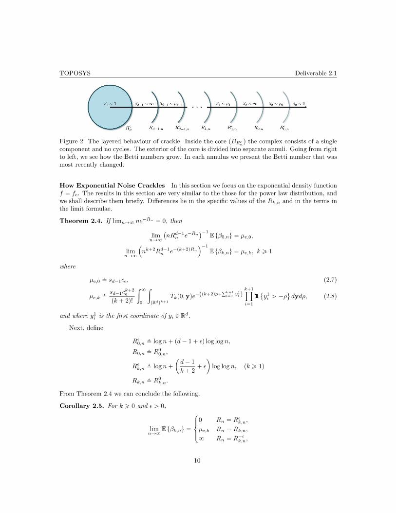
Theorem 2.2 and Corollary 2.3 reveal that the crackling behaviour is organized into separate‘layers’, see Figure 2. Dividing Rd into a sequence of annuli at radii

Rε0,n " R0,n " Rε1,n " R1,n " ¨ ¨ ¨ " Rεd´1,n " Rd´1,n " Rcn,

we observe a different behaviour of the Betti numbers in each annulus. We shall briefly review thebehaviour in each annulus, in a decreasing order of radii values. The following description is mainlyqualitative, and refers to expected values only.

• rRε0,n,8q - there are hardly any points (βk „ 0, 0 ď k ď d´ 1).

• rR0,n, Rε0,nq - points start to appear, and β0 „ µp,0. The points are very few and scattered,

so no cycles are generated (βk „ 0, 1 ď k ď d´ 1).

• rRε1,n, R0,nq - the number of components grows to infinity, but no cycles are formed yet(β0 „ 8, and βk “ 0, 1 ď k ď d´ 1).

• rR1,n, Rε1,nq - a finite number of 1-dimensional cycles show up, among the infinite number of

components (β0 „ 8, β1 „ µp,1, and βk “ 0, 1 ď k ď d´ 1).

• rRε2,n, R1,nq - we have β0 „ 8, β1 „ 8, and βk „ 0 for k ě 1.

This process goes on, until the pd´ 1q-dimensional cycles appear -

• rRd´1, Rεd´1q - we have βd´1 „ µp,d´1 and βk „ 8 for 0 ď k ď d´ 2.

• rRcn, Rd´1q - just before we reach the core, the complex exhibits the most intricate structure,

with βk „ 8 for 0 ď k ď d´ 1.

Note that there is a very fast phase transition as we move from the contractible core to thefirst crackle layer. At this point we do not know exactly where and how this phase transition takesplace. A reasonable conjecture would be that the transition occurs at Rn “ n1α (since at thisradius the term nR´αn that appears in Theorem 2.2 changes its limit, affecting the limiting Bettinumbers). However, this remains for future work.

9


Figure 2: The layered behaviour of crackle. Inside the core (BRcn) the complex consists of a single

component and no cycles. The exterior of the core is divided into separate annuli. Going from rightto left, we see how the Betti numbers grow. In each annulus we present the Betti number that wasmost recently changed.

How Exponential Noise Crackles In this section we focus on the exponential density functionf “ fe. The results in this section are very similar to the those for the power law distribution, andwe shall describe them briefly. Differences lie in the specific values of the Rk,n and in the terms inthe limit formulae.

Theorem 2.4. If limnÑ8 ne´Rn “ 0, then

limnÑ8

`

nRd´1n e´Rn

˘´1 E tβ0,nu “ µe,0,

limnÑ8

´

nk`2Rd´1n e´pk`2qRn

¯´1

E tβk,nu “ µe,k, k ě 1

where

µe,0 fi sd´1ce, (2.7)

µe,k fisd´1c

k`2e

pk ` 2q!

ż 8

0

ż

pRdqk`1

Tkp0,yqe´ppk`2qρ`

řk`1i“1 y

1i qk`1ź

i“1

1

y1i ą ´ρ

(

dydρ, (2.8)

and where y1i is the first coordinate of yi P Rd.

Next, define

Rε0,n fi log n` pd´ 1` εq log log n,

R0,n fi R00,n,

Rεk,n fi log n`

ˆ

d´ 1

k ` 2` ε

˙

log log n, pk ě 1q

Rk,n fi R0k,n.

From Theorem 2.4 we can conclude the following.

Corollary 2.5. For k ě 0 and ε ą 0,

limnÑ8

E tβk,nu “

$

’

&

’

%

0 Rn “ Rεk,n,

µe,k Rn “ Rk,n,

8 Rn “ R´εk,n,

10


As in the power-law case, Theorem 2.4 implies the same ‘layered’ behaviour, the only differencebeing in the values of Rk,n. From examining the values of Rc

n, and Rk,n it is reasonable to guessthat the phase transition in the exponential case occurs at Rn “ log n.

Gaussian Noise Does Not Crackle Simplicial complexes built over vertices sampled fromthe standard Gaussian distribution exhibit a completely different behaviour to that we saw in thepower-law and exponential cases. Define

Rε0,n fia

2 log n` pd´ 2` εq log log n,

then

Theorem 2.6. If f “ fg, ε ą 0, and Rn “ Rε0,n, then for 0 ď k ď d´ 1

limnÑ8

E tβk,nu “ 0.

Note that in the Gaussian case limnÑ8

`

Rε0,n ´Rcn

˘

“ 0. This implies that as nÑ 8 we havethe core which is contractible, and outside the core there is hardly anything. In other words, theball placed around every new point we add to the sample immediately connects to the core, andthus, the Gaussian noise does not crackle.

2.2 Stationary Point Processes

The work in this section is also concerned with the homology of random simplicial complexes,although with a novel and - from the point of view of both theory and applications – importantchange of emphasis. Previous papers on simplicial complexes built over random point sets havealways assumed that the points were either independent, identically distributed (iid) observationsfrom some underlying distribution on Rd, or points of a (typically non-homogeneous) Poisson pointprocess. Our aim in this paper is to investigate situations in which the points are chosen from ageneral point process, in which the points exhibit dependence such as attraction or repulsion. Fromthe point of view of topological data analysis (TDA) our results, which show that local dependenciescan have a major affect on the growth rates of topological quantifiers such as Betti numbers, impacton considerations of model (non) robustness for statistical inference in TDA.

To start being a little more specific, given a point process (i.e. locally finite random countingmeasure) Φ on Rd, recall that the random geometric graph GpΦ, rq, for r ą 0, is defined as thegraph with vertex set Φ and (undirected) edge set tpX,Y q P Φ2 X ´ Y ď ru. The properties ofrandom geometric graphs when Φ is a Poisson point process or a point process of iid points havebeen analysed in detail (cf. [28]), and recently interest has turned to the richer topic of randomsimplicial complexes built over these point sets. We shall be concerned with Cech and Vietoris-Ripscomplexes. Let Bxpεq denote the ball of radius ε around x, and P “ tx1, x2, . . .u be a collection ofpoints in Rd.

Both of these (related) complexes are important in their own right, with the Cech complexbeing of particular interest since it is known to be homotopy equivalent to the random Boolean setŤ

xPP Bxpεq which appears in integral geometry (e.g. [30]) and continuum percolation (e.g. [21]).We shall concentrate in this paper on the ranks of the the homology groups – i.e. the Betti numbers– of these complexes in the random scenario.

A complementary approach to studying the topological structure of simplicial complexes is via(non-smooth) Morse theory, and here results for Poisson process generated complexes are given in

11


[5]. In fact, the local structure of Morse critical points is often more amenable to computation thanthe global structure of the Betti numbers.

There are some recurring themes and techniques in the analysis of Betti numbers and Morsecritical points, which are intimately related to the subgraph and component counts of the corre-sponding random geometric graph. Thus, from the purely technical side, much of this paper will beconcerned with the intrinsically interesting task of extending the results of [28, Chapter 3] on sub-graph and component counts of Poisson point processes to more general stationary point processes.Subgraph counts of a random geometric graph are an example of U-statistics of point processes.Hence, apart from their applications in this article, our techniques to study subgraph counts ofrandom geometric graph over general stationary point processes could be useful to derive asymp-totics for many other translation and scale invariant U-statistics of point processes (For example,the number of k-simplices in a Cech or Vietoris-Rips complexes). Also, the results on subgraphcounts are used to derive results about clique numbers, maximum degree and chromatic number ofthe random geometric graph on Poisson or i.i.d. point process ([28, Chapter 6]) and with a similarapproach, our results can be used to derive asymptotics for clique numbers, maximum degree andchromatic number of random geometric graphs over general stationary point processes.

A sampler of some of our main results follows a little necessary notation.

2.2.1 Some notation

We use |.| to denote Lebesgue measure and . for the Euclidean norm on Rd. Depending on context,|.| will also denote the cardinality of a set. As above, we denote the ball of radius r centred at

x P Rd by Bxprq. For ξ “ px1, . . . , xkq P Rdk, let Bξprq “Ťki“1Bxiprq, hpξq “ hpx1, . . . , xkq for

h Rdk Ñ R and dξ “ dx1 . . . dxk. Let 1 “ p1, . . . , 1q. We also use the standard Bachman-Landaunotation for asymptotics1, and say that a sequence of events An, n ě 1 occurs with high probability(whp) if P tAnu Ñ 1 as nÑ8.

2.2.2 A result sampler

We shall now describe, without (sometimes important) precise technical conditions, some of ourmain results. Full details are given in the main body of the paper. We start with Φ, a unit intensity,stationary point process on Rd, and set 2

Φn “ ΦX”

ń1d

2,n1d

2

ıd

. (2.9)

1That is, for sequences an and bn of positive numbers, we write

an “ opbnq ðñ for any c ą 0 there is a n0 such that an ă cbn for all n ą n0,

an “ Opbnq ðñ there exists a c ą 0 and a n0 such that an ă cbn for all n ą n0,

an “ ωpbnq ðñ for any c ą 0 there is a n0 such that an ą cbn for all n ą n0,

an “ Ωpbnq ðñ there exists a c ą 0 and a n0 such that an ą cbn for all n ą n0,

an “ Θpbnq ðñ an “ Opbnq and an “ Ωpbnq

2Note that our basic setup is a little different different to that of all the earlier papers mentioned above. To compareour results with existing ones on Poisson or iid point processes, note that rdn in our results typically corresponds tonrdn elsewhere. For a general (non-Poisson) point process, (2.9) provides a more natural setting.

12


Let

βk pCpΦn, rqq , βk pRpΦn, rqq ,

respectively, denote the k-th Betti numbers of the Cech and Vietoris-Rips complexes based on Φn.In addition, let CkpΦn, rq denote the set of Morse critical points of index k for the distance

function

dnpxq “ minXPΦn

x´X,

and set

NkpΦn, rq “ |tc P CkpΦn, rq dnpcq ď ru| .

This paper is concerned with the behavior, as n Ñ 8, of βk pCpΦn, rnqq, βk pRpΦn, rnqq,NkpΦn, rnq and χpCpΦn, rnqq, where χ denotes the Euler characteristic. In particular, we shallprovide closed form expressions for the asymptotic, normalised, first moments of these variables,along with bounds for second moments for most of them.

Throughout the remainder of this subsection we shall assume that Φ is stationary, unit mean,and negatively associated. Additional side conditions may also need to hold, but we shall not statethem here. Two simple examples for which everything works are provided by the Ginibre pointprocess and the simple perturbed lattice. Many of the results hold for various other sub-classes ofpoint processes as well, but our non-specific blanket assumptions allow for ease of exposition. Wedivide the results into three classes, depending on the behavior of rn.I. Sparse regime: rn Ñ 0. Note that since the points of Φ only generate edges and faces of theCech and Vietoris-Rips complexes CpΦn, rq and RpΦn, rq when they are distance less than r apart,and since Φ has, on, average, only one point per unit cube, if r is small we expect that both of thesecomplexes will be made up primarily of the isolated points of Φ. We describe this fact by callingthis the ‘sparse’ regime.

In this setting,

Etβ0pCpΦn, rnqu “ Etβ0pRpΦn, rnqu “ Θpnq

and for k ě 1, there exist functions fkprq ” 1 or fkprqÑ0, as r Ñ 0, depending on the precisedistribution of Φ and on the index k, such that

EtβkpCpΦn, rnqu “ Θpnrdpk`1qn fk`2prnqq,

EtβkpRpΦn, rnqu “ Θpnrdp2k`1qn f2k`2prnqq, (2.10)

EtNkpΦn, rnqu “ Θpnrdkn fk`1prnqq,

and VarpNkpΦn, rnqq “ OpEtNkpΦn, rnquq, where VarpXq is the variance ofX. In addition, E

n´1χpCpΦn, rnqq(

Ñ

1.In the classical Poisson case, studied in the references given above, it is known that the same

results hold with f ” 1.Using stochastic ordering techniques, we shall also show that clustering of point processes in-

creases the functions fkprq and consequently the mean of the βk and Nk as well. Also, we know thatfor the Ginibre point process and for the zeroes of Gaussian entire functions, fkprq “ rkpk´1q. Thus,

13


there is a systematic difference between the scaling limits for Poisson and at least some negativelyassociated point processes.II. Thermodynamic regime: rdn Ñ β P p0,8q. In this regime an edge between two pointsin Φ, which are, in a rough sense, an average distance of one unit apart, will be formed if theymanage to get within a distance β1d of one another. Since, in most scenarios, there should be areasonable probability of this happening, we expect to see quite a few edges and, in fact, simplicesand homologies of all dimensions. Indeed, this is the case, and the main result in this regime isthat topological complexity grows at a rate proportional to the number of points, in the sense that

EtβkpCpΦn, rnqu “ Θpnq,

with identical results for EtβkpRpΦn, rnqqu and EtNkpΦn, rnqu. In addition, VarpNkpΦn, rnqq “OpEtNkpΦn, rnquq and

E

n´1χpCpΦn, rnqq(

Ñ 1`dÿ

k“1

p´1qkνkpΦ, βq,

where the νkpΦ, βq are defined in Theorem 2.22. Since there is no appearance in these results of ananalogue to the f of (2.10), the normalisations here have the same orders as in the Poisson and iidcases.III. Connectivity regime: rdn “ Θplog nq. Clearly, if rn is large enough, there comes a point(which we call the contractibility radius) beyond which all the points of Φn will connect with theothers and both the Cech and Vietoris-Rips simplices will become trivial, in the sense that thegraph over the points will be totally connected, and so the various simplicial complexes will becontractible to a single point. (This is certainly the case if rn “

?dn1d.) The question, then, is

“how large is large enough”.It turns out that in the current scenario of negative association there exist case dependent

constants C such that for, rn ě Cplog nq1d, CpΦn, rnq is contractible whp as n Ñ 8. In thespecific cases of the Ginibre process or zeroes of Gaussian entire functions, this happens earlier,and rn “ Θpplog nq14q is the radius for contractibility of the Cech complex. As a trivial corollary,it follows that, whp, χpCpΦn, rnqq “ 1 when rn is the radius of contractibility. Further, for theGinibre process, rn “ Θpplog nq14q is also the critical radius for k-connectedness of the Vietoris-Ripscomplex.

2.2.3 Some implications for topological data analysis

Perhaps the core tool of TDA is persistent homology, as visualised through barcodes and persistencediagrams (cf. [8, 13, 16, 32]). While here is not the place to go into the details of persistent homology,it can be described reasonably simply in the setting of this paper. For a given n, and a collection ofpoints Φn, consider the collections of Cech (or Vietoris-Rips) complexes CpΦn, rq built over thesepoints, as r grows. Initially, CpΦn, 0q will contain only the points of Φn. However, as r increases,different homological entities (cycles of differing degree) will appear and, eventually, disappear. If toeach such phenomenon we assign an interval starting at the birth time and ending at the death time,then the collection of all of these intervals is a representation of the persistent homology generatedby Φn and is known as its ‘barcode’. The individual intervals are referred to as ‘bars’.The Bettinumbers βkpCpΦn, rqq therefore count the number of bars related to k-cycles active at ‘connectiondistance’ r.

14


Heuristics and (unpublished) simulations indicate that bars of regular or negatively correlatedpoint processes start later and vanish earlier than those for Poisson point process. Some of ourresults confirm this heuristic. For example, using the results above it is easy to see that non-trivial homology groups of Cech and Vietoris-Rips complexes start to appear once rn satisfies

rdpk`1qn fk`2prnq “ ωpn´1q. For the Poisson case this requires only rn “ ωpn´1dpk`1qq. Since,

typically, fprq Ñ 0 as r Ñ 0, we therefore generally need larger radii for non-trivial homologyto appear. The disappearance of homology is harder, however, and in general our results onconnectivity cannot confirm the heuristic. However, for the Ginibre point process and zeroes ofGEF in R2, they do show that non-trivial topology vanishes at rn “ ωpplog nq14q as opposed toωpplog nq12q for a two dimensional Poisson process.

As for implications to TDA, applied topologists are beginning to appreciate the fact that stochas-ticity underlies their data as a consequence of sampling, and are beginning to build statistical modelsto allow parameter estimation and inference (e.g. [7, 9, 23, 31]). The results of this paper showthat small changes in model structure (such as the introduction of attraction and repulsion betweenpoints in a data cloud) can have measurable effects on topological behaviour.

2.2.4 Subgraph and component counts in random geometric graphs

Recall that for a point set Φ and radius r ą 0, the geometric graph GpΦ, rq is defined as the graphwith vertex set Φ and edge-set tpX,Y q X ´ Y ď ru. We shall work with restrictions of Φ to

a sequence of increasing windows Wn “ rń1d

2 , n1d

2 sd, along with a radius regime trn ą 0uně1,setting Φn :“ ΦXWn. The choice of the radius regime will impact on the asymptotic properties ofthe geometric graph when the points of Φ are those of a point process.

Let Γ be a connected graph on k vertices. In this section we shall be interested in how oftenΓ appears (up to graph isomorphisms) in a sequence of geometric graphs Gn “ GpΦn, rnq, andhow often among such appearances it is actually isomorphic to a component of Gn, viz. it is aΓ-component of Gn. For graphs built over Poisson and iid processes, we know from [28, Chapters3,13] that no Γ-components exist when nprdnq

k´1 Ñ 0 (|Γ| “ k), but that they do appear whennprdnq

k´1 Ñ 8. The Γ-components continue to exist even when rdn “ oplog nq and vanish whenrdn “ ωplog nq, which is the threshold for connectivity of the graph.

In this section, we shall show, among other things, that the threshold for formation of Γ-components for negatively associated processes with rn Ñ 0 is nprdnq

k´1fkprnq Ñ 8, for functionsfk which typically satisfy fkprq Ñ 0 as r Ñ 0, and so is higher than in the Poisson case. Thesecomponents continue to exist even when rdn Ñ β ą 0. The threshold for the vanishing of componentswill be treated in the next section.

The reader should try to keep this broader picture in mind as she wades through the variouslimits of this section.

2.2.5 Some notation and a start

As above, let Γ be a connected graph on k vertices, k ě 1, and tx1, . . . , xku a collection of k pointsin Rd. Introduce the (indicator) function hΓ Rdk ˆ R` Ñ t0, 1u by

hΓpξ, rq :“ 1rGptx1, . . . , xku, rq » Γs, (2.11)

15


where » denotes graph isomorphism and 1 is the usual indicator function. For a fixed sequencetrnu set

hΓ,npξq :“ hΓpξ, rnq, (2.12)

and, for r “ 1, write

hΓpξq :“ hΓpξ, 1q (2.13)

Moving now to the random setting, in which Φ is a simple point process with k-th intensitiesρpkq, we say that Γ is a feasible subgraph of Φ if

ż

pRdqkhΓpξqρ

pkqpξq dξ ą 0.

Thus, Γ is a feasible subgraph of Φ if the αpkq measure of finding a copy of it (up to graphhomomorphism) in GpΦ, 1q is positive. In most cases, feasibility will hold because ρpkqpξq ą 0 a.e.or at least on a large enough set.

We shall be interested in the the number of Γ-subgraphs, GnpΦ,Γq, and number of Γ-components,JnpΦ,Γq, of Φn, which are defined as follows3:

GnpΦ,Γq :“1

k!

ÿ

XPΦpkqn

hΓ,npXq (2.14)

JnpΦ,Γq :“1

k!

ÿ

XPΦpkqn

hΓ,npXq1rΦnpBXprnqq “ ks.

Note that Jn considers graphs based on vertices in Φn only, viz. all vertices that lie in Wn. Sucha graph, however, may have vertices within distance rn of a point in the complement of Wn, andso actually be part of something larger. To account for this boundary effect, we introduce anadditional variable, which does not count such “boundary crossing” graphs. This is given by

JnpΦ,Γq :“1

k!

ÿ

XPΦpkqn

hΓ,npXq1rΦpBXprnqq “ ks. (2.15)

We shall see later that in the sparse and thermodynamic regimes the differences between Jn andJn disappear in asymptotic results. Nevertheless, both are needed for the proofs.

The key ingredient in obtaining asymptotics for sub-graph counts and component counts arethe following closed-form expressions, which are immediate consequences of the Campbell-Meckeformula.

EtGnpΦ,Γqu “1

k!

ż

Wkn

hΓ,npξq ρpkqpξq dξ, (2.16)

EtJnpΦ,Γqu “1

k!

ż

Wkn

hΓ,npξqP!ξtΦnpBξprnqq “ 0u ρpkqpξq dξ. (2.17)

3In the terminology of [28], GnpΦ,Γq denotes the number of induced Γ´ subgraphs of GpΦ, rq and not the numberof subgraphs of GpΦ, rq isomorphic to Γ. However, it is easy to see that the latter is a finite linear combination ofthe number of induced subgraphs of the same order.

16


Much of the remainder of this section is based on obtaining asymptotic expressions for these integralsin terms of basic point process parameters in the sparse and thermodynamic regimes, as well aslooking at bounds on variances. We shall consider the connectivity regime only in the followingsection on Betti numbers. Our results here extend those of [28, Chapter 3] for Poisson and iidprocesses, and the general approach of the proofs is thus similar.

2.2.6 Sparse regime: rn Ñ 0

The intuition behind the following theorem is that in the sparse regime it is difficult to find Γ-subgraphs in a random geometric graph, and even more unlikely that any such subgraph will haveanother point of the point process near it. This implies that any such subgraph will actually be acomponent of the full graph, disconnected from other components.

Theorem 2.7. Let Φ be a stationary point process in Rd of unit intensity and Γ be a feasi-ble connected graph of Φ on k vertices. Let ρpkq be almost everywhere continuous. Assume thatρpkqp0, . . . , 0q “ 0, and that there exist functions fkρ R` Ñ R` and gkρ pB0pkqq

k Ñ R` such that

ρpkqpryq “ Θpfkρ prqq and limrÑ0

ρpkqpryq

fkρ prq“ gkρpyq,

for all y of the form y “ p0, y2, . . . , ykq. Further, assume that fk`1 “ Opfkq as r Ñ 0 and gkρ isalmost everywhere continuous. Let rn Ñ 0. Then,

limnÑ8

EtGnpΦ,Γqunr

dpk´1qn fkprnq

“ limnÑ8

EtJnpΦ,Γqunr

dpk´1qn fkprnq

(2.18)

“ µ0pΦ,Γq

:“

#

1 k “ 1,1k!

ş

Rdpk´1q hΓpyqgkρpyq dy k ě 1.

If ρpkqp0, . . . , 0q ą 0, then the same result holds with fkρ ” 1 and gkρ ” ρpkqp0, . . . , 0q.

Before turning to the proof of the theorem we shall make a few points about its conditions, andprovide some examples. Throughout we assume that all point processes are normalized to haveunit intensity.1: Note that the theorem does not guarantee the positivity of µ0pΦ,Γq.2: f1prq ” 1 for all stationary point processes of unit intensity since, in this case, ρp1q ” 1.3: It is easy to check that if Φ is α-negatively associated or α-super-Poisson, then the conditionfk`1 “ Opfkq as r Ñ 0 is satisfied.4: In the case ρkp0, . . . , 0q “ 0 for k ě 2, even if we cannot find appropriate fk or gkρ , it is still true

that EtGnpΦ,Γqu “ opnrdpk´1qn q.

5: If Φ is only Zd-stationary (as is the case with perturbed lattices), then it will be clear that (2.19)still holds, but with

µ0pΦ,Γq :“1

k!

ż

r0,1sd

ż

Rdpk´1q

hΓpx,yqgkρpx,yq dx dy.

6: For a homogeneous Poisson point process, the theorem holds with fk ” 1 and gkρ ” 1, recovering[28, Prop. 3.1].

17


7: If Φ ěα´w Φp1q, then for all k ě 1, ρpkq ě ρpkqp1q ” 1 and hence fk ” 1 and also µ0pΦ,Γq ą 0.

Examples of point processes in this class are all super-Poisson perturbed lattices and permanentalpoint processes.8: For a perturbed lattice Φ with perturbation kernel N P t0, . . . ,Ku a.s., ρpkqp0, . . . , 0q ą 0 iffk ď K. In this case, µ0pΦ,Γq ą 0 for a connected graph Γ on k vertices. For connected graphs

Γ on k vertices with k ą K, nr´dpk´1qn EtGnpΦ,Γqu Ñ 0. For sub-Poisson perturbed lattices, the

existence of fk depends on the perturbation kernel. However, for high values of k, it is clear thatthe scaling for sub-Poisson perturbed lattices will differ significantly from that of the Poisson case.9: From [24, Theorem 1.1] for the zeroes of Gaussian entire function and calculations similar to [4,Theorem 4.3.10] for the Ginibre point process, one can check that in both cases

ρkpx1, . . . , xkq “ Θ´

ź

iăj

xi ´ xj2¯

.

Hence, fkprq “ Θprkpk´1qq for these processes.The following corollary follows easily from the ordering of the joint intensities of the point

processes.

Corollary 2.8. Let Φi, i “ 1, 2, be two stationary point processes and fkρi , gkρi correspond to the

functions of Theorem 2.7. If Φ1 ďα´w Φ2, then fkρ1 ď fkρ2 . If fkρ1 ” fkρ2 , then gkρ1 ď gkρ2 , and henceµ0pΦ1,Γq ď µ0pΦ2,Γq for a connected graph Γ that is feasible for both Φ1 and Φ2.

2.2.7 Thermodynamic regime: rdn Ñ β

Theorem 2.9. Let Φ be a stationary point process in Rd of unit intensity and Γ be a feasibleconnected graph of Φ on k vertices. Assume that ρpkq is almost everywhere continuous, and letrdn Ñ β ą 0 and y “ p0, y2, . . . , ykq. Then,

limnÑ8

EtGnpΦ,Γqun

“ µβpΦ,Γq

:“

#

1 k “ 1,βk´1

k!

ş

Rdpk´1q hΓpyqρpkqpβ

1dyq dy k ě 2,

(2.19)

limnÑ8

EtJnpΦ,Γqun

“ γβpΦ,Γq

:“

$

’

’

&

’

’

%

P!O

!

ΦpBOpβ1d qq “ 0

)

k “ 1,

βk´1

k!

ş

Rdpk´1q hΓpyqρpkqpβ

1dyq

ˆP!

β1d y

!

ΦpBβ

1d ypβ

1d qq “ 0

)

dy k ě 2.

(2.20)

If Φ is a negatively associated point process with P!

ΦpBξpβ1d qq “ 0

)

ą 0 for almost every ξ P

B0pβ1d kqk, then γβpΦ,Γq ą 0.

Again, before turning to the proof, we make some observations about the theorem:1: The positivity of γβpΦ,Γq is not immediate. For an example in which this does not hold, let Φ0

be a Poisson point process of unit intensity in Rd, Φi, i ě 1 iid copies of the point process of 4 iid

18


uniformly distributed points in BOpβ1d 2q, and define the Cox point process,

Φ :“ď

XiPΦ0

tXi ` Φiu.

Clearly, for all X P Φ, P!

ΦpBXpβ1d q ě 4

)

“ 1.

Now take rdn ” β and Γ a triangle, and note that JnpΦ,Γq “ 0 for all n ě 1 and so γβpΦ,Γq “ 0,even though all the assumptions of Theorem 2.9 are satisfied.2: As in Corollary 2.8, Φ1 ďα´w Φ2 implies that µβpΦ1,Γq ď µβpΦ2,Γq. However, as the previousexample shows, the situation for γβpΦ,Γq is somewhat more complicated.3: If |Γ| “ 1, then JnpΦ,Γq is the number of isolated nodes in the Boolean model of balls of radii βcentred on the points of Φ The Palm measure of a determinantal point process is also determinantaland in particular, for the Ginibre process, ρ!p1qpzq “ 1´ e´z

2

. Using this explicit structure, it canbe shown that, for small enough β,

γβpΦGin,Γq ě 1´ πβ2 ` πp1´ e´β2

q ą 1´ πβ2 Òpπ2β4q “ γβpΦPoi,Γq,

and hence the inequality for the γβ could be reversed in the thermodynamic regime for even nega-tively associated point processes as compared to the sparse regime.

2.2.8 Variance bounds for the sparse and thermodynamic regimes

The crux of the second moment bounds lies in the fact that, up to constants, variances are essentiallybounded above (below) by expectations for negatively associated (associated) point processes. (Itis simple to check that Varp.q “ ΘpEt.uq for the Poisson process, which is both negatively associatedand associated (cf. [28, Chapter 3]).) We, however, shall need to extend these inequalities to graphvariables, and this is the content of this section.

Theorem 2.10 (Covariance bounds in sparse regime). Let Γ and Γ0 be two feasible connectedgraphs on k and l (k ě l ě 2) vertices, respectively, for a stationary point process Φ with almosteverywhere continuous joint densities. Let Φ satisfy the assumptions of Theorem 2.7 and assumethat the f j and gjρ exist for all j ď k ` l. Further, let rn Ñ 0 and µ0pΦ,Γq ą 0.

1. If Φ is α-negatively associated, then

Cov pGnpΦ,Γq, GnpΦ,Γ0qq “ OpEtGnpΦ,Γquq.

2. If Φ is α-associated, then

Cov pGnpΦ,Γq, GnpΦ,Γ0qq “ ΩpEtGnpΦ,Γquq.

Unlike the sparse regime, subgraph counts and component counts have different limits in thethermodynamic regime and hence we need variance bounds on component counts in the thermody-namic regime.

Theorem 2.11 (Variance bounds in the thermodynamic regime). Let Φ be a stationary pointprocess in Rd of unit intensity and Γ be a feasible connected graph of Φ on k vertices. Assume thatρpkq is almost everywhere continuous. Let rdn Ñ β ą 0 and γβpΦ,Γq ą 0.

1. If Φ is negatively associated, then Var´

JnpΦ,Γq¯

“ OpEtJnpΦ,Γquq.

2. If Φ is associated, then Var´

JnpΦ,Γq¯

“ ΩpEtJnpΦ,Γquq.

19


2.2.9 Phase transitions in the sparse and thermodynamic regimes

So far, we have concentrated on the asymptotic behaviour of the expectations of the numbers ofdifferent types of subgraphs that appear in the random graph associated with a point process. Inthis section we shall combine expectations on first and second moment to obtain results about thesenumbers themselves, looking at probabilities that they are non-zero, as well as L2 and almost sureresults about growth and decay rates. The main theorem of this section is the following:

Theorem 2.12. Let Φ be a stationary point process with almost everywhere continuous joint den-sities and Γ a feasible connected graph for Φ on k vertices.1: Let Φ satisfy the assumptions of Theorem 2.7 with µ0pΦ,Γq ą 0. Let rn Ñ 0.

(a) If nrdpk´1qn fkprnq Ñ 04, then P tGnpΦ,Γq ě 1u Ñ 0.

(b) If Φ is α-negatively associated and nrdpk´1qn fkprnq Ñ β for some 0 ă β ă 8, there there

exists a finite C (dependent on the process but not on Γ) for which

limnÑ8

P tJnpΦ,Γq ě 1u ě

„

1`C

βµ0pΦ,Γq

´1

.

(c) If Φ is α-negatively associated and nrdpk´1qn fkprnq Ñ 8, then

JnpΦ,Γq

nrdpk´1qn fkprnq

L2Ñ µ0pΦ,Γq.

2: Let Φ be a negatively associated point process satisfying the assumptions of Theorem 2.9 withγβpΦ,Γq ą 0. Let rdn Ñ β. Then,

JnpΦ,Γq

nL2Ñ γβpΦ,Γq.

Since Jn is a Kd-Lipschitz functional of counting measures for a constant Kd depending only onthe dimension d (see [28, Proof of Theorem 3.15]), the result in (2) above can be strengthened toa.s. convergence for stationary determinantal point processes by using the concentration inequalityin [27, Theorem 3.6]. We leave the proof, which is not hard, to the reader.

Theorem 2.13. Let Φ be a stationary determinantal point process of unit intensity and Γ a feasibleconnected graph for Φ on k vertices. Let rdn Ñ β ą 0. Then, for γβpΦ,Γq as defined in (2.20),

JnpΦ,Γq

na.s.Ñ γβpΦ,Γq, as nÑ8.

2.2.10 Betti numbers of random geometric complexes

This is really the main section of the paper, giving, as it does, results about the homology of randomgeometric complexes through their Betti numbers. Despite this, it will turn out that, as mentionedearlier, the hard work for the proofs has already been done in the previous section.

4Note that neither this assumption nor the one in 1(b) can hold for k “ 1, as f1prq ” 1. Hence the statementsdo not say anything in these two cases.

20


We shall start with a review of the basic topological notions needed to formulate our results,along with an explanation of the connections between Betti numbers of random complexes andcomponent numbers of random geometric graphs. This connection was established and exploitedin [19, 20] to extract theorems for Betti numbers from those for the component counts of randomgeometric graphs.

2.2.11 Topological preliminaries

Recall the well-known definitions of the Cech and Vietoris-Rips complexes and their faces, and thatthe dimension of a face σ is |σ| ´ 1. Recall also that the edges of the random geometric graphGpΦ, rq are the 1-dimensional faces of CpΦ, rq or RpΦ, rq.

Now, however, we require some additional terminology.The Vietoris-Rips complex RpΦ, rq is also called the clique complex (or flag complex) of GpΦ, rq,

as the faces are cliques (complete subgraphs) of the 1´ dimensional faces. Let HkpCpΦ, rqq andHkpRpΦ, rqq, respectively, denote the k-th simplicial homology groups of the random Cech andVietoris-Rips complexes. (We shall take our homologies over the field Z2, but this will not be im-portant.) In this section we shall be concerned with asymptotics for the Betti numbers βkpCpΦn, rqqand βkpRpΦn, rqq, (i.e. the ranks of the homologies) and through them the appearance and disap-pearance of homology groups.

Next, let Pk be the pk ` 1q-dimensional cross-polytope in Rk`1, containing the origin, anddefined to be the convex hull of the 2k ` 2 points t˘eiu, where e1, . . . , ek`1 are the standardbasis vectors of Rk`1. The boundary of Pk, which we denote by Ok, is a k-dimensional simplicialcomplex, homeotopic to a k-dimensional sphere. In terms of simplicial homology, the existence ofsubsimplices isomorphic to Ok is the key to understanding k-cycles and so the k-th homology. Infact, from [18, Lemma 5.3] we know that, because of the distance relationships between the verticesof a Vietoris-Rips complex, any non-trivial element of the k-dimensional homology HkpRpΦ, rqqarises from a subcomplex on at least 2k ` 2 vertices. If it has only 2k ` 2 vertices, then it will beisomorphic to Ok.

Now let Γjk, j “ 1, . . . , nk (nk ă 8) be an ordering of the different graphs that arise whenextending a (k ` 1)-clique (i.e. a k-dimensional face) to a minimal connected subgraph on 2k ` 3vertices. Thus, the Γjk are all graphs on 2k ` 3 vertices, having

`

k`12

˘

` k ` 2 edges.

Finally, for a given finite graph Γ, let GpΦ,Γq denote the number of subgraphs of GpΦ, rq that areisomorphic to Γ. However, as explained in 3, GpΦn,Γq is a finite linear combination of GnpΦ,Γ

1

q’swith Γ

1

’s being of the same order as Γ.Then [18, Lemma 5.3] and a dimension bound in [19, (3.1)]) imply the following crucial inequality

linking Betti numbers to component and subgraph counts in Vietoris-Rips complexes for k ě 1;

JpΦ, Okq ď βkpRpΦ, rqq ď JpΦ, Okq `nkÿ

j“1

GpΦ,Γjk,2k`3q. (2.21)

A related inequality holds for Cech complexes. Let Γk be the graph on k vertices such that anyk´ 1 vertices form a pk´ 1q-clique but Γk is not a k-clique. Any collection of vertices X for whichGpX, rq » Γk is said to form an empty pk ´ 1q-simplex. Let Γ

1

k be the graph of a pk ´ 1q-clique

with an extra edge attached to two vertices and Γ2

k be the graph of a pk ´ 1q-clique with a path of

length 2 attached to one of the vertices. Both Γ1

k and Γ2

k are graphs of order k ` 1. The we have

21


the following combinatorial inequality from [20, (5)] for k ě 1:

JpΦ,Γk`2q ď βkpCpΦ, rqq ď JpΦ,Γk`2q `GpΦ,Γ1

k`2q `GpΦ,Γ2

k`2q. (2.22)

With these combinatorial inequalities in hand, we are now ready to develop limit theorems for theBetti numbers of the random Cech and Vietoris-Rips complexes (Section 2.2.12) as well as findthresholds for vanishing and non-vanishing of homology groups (Section 2.2.13).

2.2.12 Expectations of Betti numbers

We return now to the setting of a stationary point process Φ in Rd and the sequence of finite pointprocesses Φn. Our results all follow quite easily from the corresponding limit theorems in Section2.2.4, and we continue to use the notation of that section without further comment.

The underlying heuristic is that in the sparse regime the order is determined by the order of theminimal structure involved in forming homology groups, which is Ok for the random Vietoris-Ripscomplex and Γk for the random Cech complex. Using Theorem 2.7, it is easy to see that these arethe leading order terms and that the G and G terms in both (2.21) and (2.22) are, asymptotically,irrelevant. Hence, we have the following result.

Theorem 2.14 (Sparse regime: rn Ñ 0). Let Φ be a stationary point process in Rd satisfying theassumptions in Theorem 2.7 for all k ě 1. Let rn Ñ 0. Further, assume that µ0pΦ,Γkq ą 0 andµ0pΦ, Okq ą 0 for all k ě 1. Then, for all k ě 1,

limnÑ8

EtβkpCpΦn, rnqqunr

dpk`1qn fk`2prnq

“ µ0pΦ,Γk`2q,

limnÑ8

EtβkpRpΦn, rnqqunr

dp2k`1qn f2k`2prnq

“ µ0pΦ, Okq.

For k “ 0, we have that

limnÑ8

Etβ0pCpΦn, rnqqu

n“ limnÑ8

Etβ0pRpΦn, rnqqu

n“ 1.

Turning now to the thermodynamic regime, and applying the same arguments as in the previousproof, but using Theorem 2.9 in place of Theorem 2.7, we find that all the terms in (2.21) and (2.22)are of order Θpnq. This leads to the following result.

Theorem 2.15 (Thermodynamic regime: rdn Ñ β). Let Φ be a stationary point process in Rdsatisfying the assumptions in Theorem 2.9 for all k ě 1. Let rdn Ñ β P p0,8q. Further, assumethat γβpΦ,Γkq ą 0 and γβpΦ, Okq ą 0 for all k ě 1. Then, for all k ě 0,

EtβkpCpΦn, rnqqu “ Θpnq, EtβkpRpΦn, rnqqu “ Θpnq.

We note without proof that one can obtain ordering results for Betti numbers of α´w orderedpoint processes in the sparse regime analogous to Corollary 2.8 but not in the thermodynamicregime.

22


2.2.13 Thresholds for homology groups

Our aim in this subsection is to establish results about the conditions under which different homol-ogy groups appear and disappear in the homology of random complexes. We shall need to treatCech and Vietoris-Rips complexes separately, and start with results on the contractibility of these.We follow these with the key results of the section, on thresholds for the appearance and disappear-ance of homology groups. These results also show that γ-weakly sub-Poisson point processes havelower vanishing thresholds for given Γ-components. As a corollary to the results on Cech complexes,we also obtain an asymptotic result on the behaviour of the Euler characteristic χpCpΦ, rq.

Recall that there are a number of equivalent definitions for Euler characteristic. However, themost natural for us at this point is

χpCpΦ, rq :“ÿ

kě0

p´1qkβkpCpΦ, rqq. (2.23)

Theorem 2.16 (Contractibility of Cech complexes). Let Φ be a stationary γ-weakly sub-Poisson

point process. Then there exists a Cd ą 0 such that for rn ě Cdplog nq1d , whp CpΦn, rnq is con-

tractible and χpCpΦn, rnqq “ 1.

With these results in hand, we can now use the bounds (2.21) and (2.22) along with a.s. existenceresults of Section 2.2.8 to complete the picture about vanishing and non-vanishing of homologygroups of Cech complexes and Vietoris-Rips complexes.

Theorem 2.17 (Thresholds for Cech complexes). Let Φ be a stationary point process satisfyingthe assumptions on its joint intensities ρpkq as in Theorems 2.7 and 2.9 for all k ě 1. Then thefollowing statements hold :

1. Let Φ be a γ-weakly sub-Poisson point process.

(a) Ifrdpk`1qn fk`2prnq “ opn´1q or rdn “ ωplognq,

then HkpCpΦn, rnqq “ 0, k ě 1, whp.

(b) If rdn “ ωplognq, then H0pCpΦn, rnqq “ 1, whp.

2. Let Φ be a negatively associated point process. Further assume that µ0pΦ,Γkq ą 0 andγβpΦ,Γkq ą 0, both for all k ě 1 and all β ą 0.

(a) Ifrdpk`1qn fk`2prnq “ ωpn´1q and rdn “ Op1q,

then HkpCpΦn, rnqq ‰ 0, k ě 1, whp.

(b) If rdn “ Op1q, then H0pCpΦn, rnqq ‰ 0, whp.

In the absence of a contractibility result for the Vietoris-Rips complex, we are unable to estimatethe second thresholds, where the homology groups vanish. Thus, we have the following less completepicture for the Vietoris-Rips complex. Since H0pCpΦn, rnqq “ H0pRpΦn, rnqq, we shall restrictourselves to only HkpRpΦn, rnqq, k ě 1, in the following theorem.

Theorem 2.18 (Thresholds for Vietoris-Rips complexes). Let Φ be a stationary point processsatisfying the assumptions on its joint intensities ρpkq as in Theorems 2.7 and 2.9 for all k ě 1.Then the following statements hold for k ě 1 :

23


1. Ifrdp2k`1qn f2k`2prnq “ opn´1q,

then HkpRpΦn, rnqq “ 0, whp.

2. Let Φ be a negatively associated point process. Further assume that µ0pΦ, Okq ą 0 andγβpΦ, Okq ą 0, both for all k ě 1 and all β ą 0. If

rdp2k`1qn f2k`1prnq “ ωpn´1q and rdn “ Op1q,

then HkpRpΦn, rnqq ‰ 0, whp.

2.2.14 Further results for the Ginibre process:

Using the special structure of the Ginibre point process, we can improve on the threshold resultsof the last section. The radius regime for contractibility of Cech complexes over the Ginibre pointprocess and zeros of GEF can be made more precise, as more is known about void probabilitiesin these cases. Once we have the contractibility results, the upper bounds for vanishing of Bettinumbers in this special case can be improved.

Theorem 2.19 (Contractibility of Cech Complexes). Let Φ be the Ginibre point process or ze-ros of GEF, then there exists a Cd ą 0 (depending on the point process) such that for rn ě

Cdplog nq14 , whp CpΦn, rnq is contractible. Hence, H0pCpΦn, rnqq “ 1, HkpCpΦn, rnqq “ 0, k ě 1

and χpCpΦn, rnqq “ 1 whp for r2n “ ωp

?lognq.

For Vietoris-Rips complexes, the contractibility result for the Ginibre point process is a conse-quence of the upper bounds for the Palm void probabilities. As in the previous subsection, oncewe have contractibility results, we can obtain upper bounds for vanishing of the Betti numbers aswell.

Theorem 2.20 (Disappearence of homology groups for Vietoris-Rips complexes). Let Φ be the

Ginibre point process. Then there exists a Cd,k ą 0 such that for rn ě Cd,kplog nq14 , we have that

whp HkpRpΦn, rnqq “ 0, k ě 1.

The proof uses the discrete Morse theoretic approach (see [14]) similar to that of [19, Theorem5.1] and the reader is referred to that proof and the appendix in [19] for missing details. As in[19, Theorem 5.1], our proof actually shows topological k-connectivity though we do not state itexplicitly to avoid defining further topological notions.

2.2.15 Morse theory for random geometric complexes

Our aim in this section is to present a collection of results looking at random geometric complexesfrom the point of view of Morse theory. This was done in considerable detail for Poisson and iidpoint processes in [5], where it was shown that a Morse theoretic approach can give an intrinsicallyricher set of results than that obtained by attacking homology directly, and that the Morse theoreticresults have, as usual, implications about Betti numbers.

We do not intend to give full proofs here, but rather to set things up in such a way that parallelsbetween the structures that have appeared in previous sections and those that are natural to theMorse theoretic approach become clear, and it becomes ‘obvious’ what the Morse theoretic results

24


will be. Full proofs would require considerable more space, but would add little in terms of insight.We note, however, that this does not make the proofs of [5] in any way redundant. On the onehand, the results there go beyond what we have here (albeit only for the Poisson and iid cases) andit is their existence that allows us to be certain that the parallels work properly.

We start with some definitions and a quick description of the Morse theoretic setting.

2.2.16 Morse Theory

Morse theory for geometric complexes is based on the distance function, dΦ : Rd Ñ R`, defined by

dΦpxq :“ minXPΦ

x´X, x P Rd.

Note that while classical Morse theory deals with smooth functions, the distance function is piece-wise linear, but non-differentiable along subspaces. The extension to the distance function ofclassical Morse theory is discussed in detail in [5], based on the definitions and results in [15], andwe shall adopt the same approach. The main difference between smooth Morse theory and thatbased on the distance function lies in the definition of the indices of critical points.

Critical points of index 0 of the distance function are the points where dΦ “ 0, which are localand global minima, and are the points of Φ. For higher indices, define the critical points as follows: A point c P Rd is said to be a critical point with index 1 ď k ď d if there exists a collection ofpoints X “ tX1, . . . , Xk`1u Ă Φpk`1q such that the following conditions hold :

1. dΦpcq “ c´Xi for all 1 ď i ď k ` 1 and dΦpcq ă c´ Y for all Y P ΦzX.

2. The points Xi, 1 ď i ď k`1 lie in general position, viz. they do not lie in a pk´1q-dimensionalaffine space.

3. c P convopXq, where convopXq denotes the interior of the convex hull formed by the points ofX.

Let CpXq denote the center of the unique pk ´ 1q-dimensional sphere (if it exists) containing thepoints of X P Φpk`1q and RpXq be the radius of the ball. The conditions in the definition of criticalpoints can be reduced to the following more workable conditions (see [5, Lemma 2.2]). A set ofpoints X P Φpk`1q in general position generates an index k critical point if, and only if,

CpXq P convopXq and ΦpBCpXqpRpXqqq “ 0.

Our interest lies in critical points which are at most at a distance r from Φ, viz. those for whichdΦpcq ď r, or, equivalently RpXq ď r. The reason for this lies in the simple fact that

d´1Φ pr0, rsq “

ď

xPΦ

Bxprq,

and, as we already noted earlier, by the nerve theorem this is homotopy equivalent to the Cechcompilex CpΦ, rq.

The following indicator functions will be required to draw the analogy between counting criticalpoints and counting components of random geometric graphs. For X P Φpk`1q, define

hpXq :“ 1rCpXq P convopXqs, hrpXq :“ 1rCpXq P convopXqs1rRpXq ď rs.

25


Note that these functions are translation and scale invariant, as were the hΓ functions defined for thesubgraph and component counts in Section 2.2.4, viz. for all x P Rd and y “ p0, y1, . . . , ykq P Rdpk`1q,

hrpx, x` ry1, . . . , x` rykq “ h1pyq.

This was the key property of hΓ used to derive asymptotics for component counts. Thus, once wemanage to represent the numbers of critical points as counting statistics of hr, the analogy withcomponent counts is made. To this end, let NkpΦ, rq be the number of critical points of index k forthe distance function dΦ that are at most at a distance r from Φ. Then,

NkpΦ, rq “ÿ

XPΦpk`1q

hrpXq1rΦpBCpXqpRpXqqq “ 0s (2.24)

The similarity between the expression for NkpΦn, rnq and Jn (cf. (2.14)) should convince the readerthat the method of proof used for component counts will also suffice for a derivation of the asymp-totics of Morse critical points. Although the void indicator term is slightly different, we can use thefact that RpXq ď r for hrpXq “ 1 to apply the techniques of Section 2.2.4 with only minor changes.

2.2.17 Limit theorems for expected numbers of critical points

As in previous sections, we shall give results for the sparse and thermodynamic regimes separately.In the Betti number results, in the sparse regime (rn Ñ 0) the scaling factor of n for Jn (see

Theorem 2.7) arose from the translation invariance of hΓ and Φ. The factor of rdpk´1qn was due to

the scale invariance of hΓ, and the factor of fkprnq came from the scaling of the joint intensitiesρpkq. Since hr is also translation and scale invariant, we work under the same assumptions on Φas in Theorems 2.7 and 2.10 with corresponding conditions hr in order to obtain asymptotics forexpected number of critical points of the distance function. The corresponding result is as follows:

Theorem 2.21 (Sparse regime). Let Φ be a stationary point process in Rd satisfying the assump-tions of Theorem 2.7 for all 1 ď k ď pd ` 1q. Let rn Ñ 0 and y “ p0, y1, y2, . . . , ykq. Then, for0 ď k ď d,

limnÑ8

EtNkpΦn, rnunrdkn f

k`1prnq“ νkpΦ, 0q

:“

#

1 k “ 0,1

pk`1q!

ş

Rdk h1pyqgk`1ρ pyq dy 1 ď k ď d.

Further, VarpNkpΦn, rnqq “ OpEtNkpΦn, rnuq for negatively associated point processes and VarpNkpΦn, rnqq “ΩpEtNkpΦn, rnuq for associated point processes.

One point that is deserving of additional comment for the proof is that, as in Theorem 2.7,we can omit the void probability term in the limit by the following reasoning: Since Rpyq ď r ifhrpyq “ 1, y “ p0, y1, . . . , ykq, we have that whenever hrnpyq “ 1,

"

ΦpBCpr

1dn yqpr

1dn qq “ 0

*

Ă

"

ΦpBCpr

1dn yqpr

1dnRpyqq “ 0

*

,

and the probability of the left event here (and hence the right as well) tends to 1. This follows fromsimilar arguments to those in the proof of Theorem 2.7.

26


Turning now to the thermodynamic regime, we saw in Theorem 2.9 that the sole scaling factorof n for component counts is due to the translation invariance of hΓ and Φ. The same remains truefor mean numbers of critical points.

Theorem 2.22 (Thermodynamic regime : rdn Ñ β.). Let Φ be a stationary point process in Rdsatisfying the assumptions of Theorem 2.9 for all 1 ď k ď pd ` 1q. Let rdn Ñ β P p0,8q andy “ p0, y1, y2, . . . , ykq. Then, for 0 ď k ď d,

limnÑ8

EtNkpΦn, rnun

“ νkpΦ, βq

:“

$

’

’

&

’

’

%

P!OpΦpBOpβ

1dRpyqqq “ 0q if k “ 0,

βk

pk`1q!

ş

Rdk h1pyqP!

β1d ypΦpB

Cpβ1d yqpβ

1dRpyqqq “ 0qρpkqpβ

1dyq dy

if 1 ď k ď d.

Further, assume that Φ is also a negatively associated point process such that

P!

ΦpBCpξqpβ1d qq “ 0

)

ą 0

for a.e. ξ “ p0, x1, . . . , xkq P B0p3β1d qk`1, and for all 1 ď k ď d. Then νkpΦ, βq ą 0 for all

0 ď k ď d.Also, VarpNkpΦn, rnqq “ OpEtNkpΦn, rnuq for negatively associated point processes and VarpNkpΦn, rnqq “ΩpEtNkpΦn, rnuq for associated point processes.

As previously, the void probability needs some attention. In this case, to show its positivity, weagain use the fact that Rpyq ď 1 if h1pyq “ 1 and hence, whenever h1pyq “ 1,

tΦpBCpβ

1d yqpβ

1d qq “ 0u Ă tΦpB

Cpβ1d yqpβ

1dRpyqq “ 0u.

Finally, we turn to a result about Euler characteristics that is not accessible from the non-Morsetheory. We already defined the Euler characteristic in terms of Betti numbers at (2.23), and showedin Theorem 2.16 that, in the connectivity regime, it is 1 with high probability. However, taking analternative, but equivalent, definition via numbers of Morse critical points, we can deduce its L1

asymptotics in the sparse and thermodynamic regimes as a corollary of the previous results in thissection. The alternative definition, which is more amenable to computations due to the boundednumber of terms in the following sum, is

χpCpΦ, rqq :“dÿ

k“0

p´1qkNkpΦ, rq.

Theorem 2.23. Let Φ be a stationary point process in Rd satisfying the assumptions of Propositions2.7 and 2.9 for all 1 ď k ď pd` 1q.

(i) If rn Ñ 0, thenn´1EtχpCpΦn, rnqqu Ñ 1.

27


(ii) If rdn Ñ β P p0,8q, then

n´1EtχpCpΦn, rnqqu Ñ 1`dÿ

k“1

p´1qkνkpΦ, βq.

(iii) If Φ is also a negatively associated point process, then the above convergences also hold in theL2-norm.

To prove the Part (iii) of the theorem, we need variance bounds, which is why we require theadditional assumption of negative association. The L2 convergence follows once it is noted thatall the terms on right hand side converge to 0 due to the variance bounds proven for negativelyassociated point processes. A slight modification of this argument handles the thermodynamicregime as well.

3 Bayesian Persistence

This work will primarily begin within the second year of the project. However, over the last twoyears, there has been some progress in using the stability of persistence diagrams in order to usethem as features in machine learning algorithms. However, many of these still depend on numerousconstants and quantities which are essentiall not estimatable. In the coming year, we will look atthe following two approaches.

3.1 Topological Features

Persistence diagrams are quite heavy to compute. Even the most efficient algorithms require mem-ory and construction of the large albeit sparse matrices as well as a reduction algorithm. Further-more, computing distances between persistence diagrams requires the Hungarian algorithm whichis cubic in the worst case. This makes it impractical for very large collections of diagrams.

Euler characteristics curves on the other hand are easy to compute but provide much lessinformation (they are however much better understood). Recent experiments have indicated thatas a feature for machine learning algorithms such as SVMs, it can prove to be as effective aspersistence diagrams. In the coming year, we will investigate this phenomenon both experimentallyand theoretically.

A natural question is under what conditions the Euler characteristic will perform “well enough”for machine learning algorithms. Another qestion is whether we can estimate important informationabout the underlying space - such as characterize the noise directly from the Euler characteristic.While early results show that the expectation of the curve is somewhat independent of the under-lying space, the variance is not, indicating that higher moments may yield additional information.

3.2 Model Selection

While the Euler characteristic is has certain advantages, it is clear that the persistence diagramcontains more information. The second line of questions we will investigate in the coming year is ifthis additional structure can be used to obtain results on model selection.

For example, as the work on crackle(heavy tailed noise) has shown, different types of noise havequalatatively different topological signatures, particularly in higher dimensions. The question wewill investigate whether this can be used to identify certain properties.

28


In addition to differentiating noise models, we will also look at power-law structures. These areubiquitous in complex systems, which leads to the question whether we can identify a qualatativetopological signature, which will go beyond looking for a linear region in data, but rather try toexplicitly find and give guarantees on the region where the behaviour is scale-free. Furthermore, byexamining topology we may be able to model such effects as anistropy through examing topologicalinvariants, for example based on local homology.

4 Smoothing

This work will primarily begin within the second year of the project. However, there are two mainapproaches which we will begin investigating.

4.1 Gaussian Kernels

The starting point for this work will be the following two papers: “Diffusion Runs Low on Per-sistence Fast” [10] and “Add Isotropic Gaussian Kernels at Own Risk: More and More ResilientModes in Higher Dimensions” [12]. The former work studies the scale-space of an image by consid-ering diffusion on the image and shows that the persistence goes to zero exponentially fast as theexperiments show. However, in the latter paper it was shown that in higher dimensions a linearnumber of persistent ghost modes can appear.

There are a number of questions we will investigate in the following year related to this phe-nomena. For example, in recent experimentst was found that topologcial features which are notintrinsic but rather depend on the embedding help in classification tasks. Does the exponentialdecay of persistence of larger scales of smoothing imply a weighting scheme to improve performancefurther?

Regarding the ghost modes which can appear, it would seem that the configuration where thisoccurs is highly non-generic. However, the stability of persistence would seem to imply that smallperturbations should not remove these ghost modes. Therefore, we will investigate if we can obtainsome probabilistic characterizations of these modes; for example, the number and height of themgiven a random point process. It seems unlikely to obtain distributions but perhaps, asymptoticresults on expectations and variances can be found.

Likewise, we will perform a similar analysis for the Euler characteristic curve.

4.2 Harmonic Forms

The second approach we will investigate will attempt to combine Hodge theory with persistence.Recall that the persistent homology of a filtration gives us a interval decomposition. If we considerthe generic situation where the filtration represents a total ordering, we also obtain a canonical basis.Therefore, we assume we are given a linear quiver of vector spaces equipped with a cannonical basis.

HkpX0q Ñ HkpX1q ÑÑ HkpXnq

Further recall that Hodge theory related the k-Laplacian with the k-dimensional homology. Thek-Laplacian is given as

Lk “ Bkδk´1 ` δkBk ` 1

29


where B and δ are the respective boundary and coboundary operators. Hodge theory tells us that

kerLk – Hk

where the k-th homology over the reals R is given in terms of harmonic form Therefore, we willinvestigate the following:

• For each vector space in the homology of the filtration, we will find the harmonic basis, thatis the set of the smoothest representatives of the canonical basis in the L2-sense.

• There exists a map between the harmonic rpresentatives which is induced from inclusion atthe chain level.

• This allows us to map forward or restrict the representatives to compare them. Further, sincethey are represented over R, we can compute an inner product. This gives a linear map whichwe can find by computing the inner product between the basis elements of the two vectorspaces.

• The singular values of this map encodes the transformations between the bases.

This type of procedure captures more of the geometry than simply the filtration but is curretnlynot well understood.

References

[1] Robert J. Adler, Omer Bobrowski, Matthew S. Borman, Eliran Subag, and Shmuel Weinberger.Persistent homology for random fields and complexes. Institute of Mathematical StatisticsCollections, 6:124–143, 2010.

[2] Lior Aronshtam, Nathan Linial, Tomasz Luczak, and Roy Meshulam. Vanishing of the tophomology of a random complex. Arxiv preprint arXiv:1010.1400, 2010.

[3] Eric Babson, Christopher Hoffman, and Matthew Kahle. The fundamental group of random2-complexes. J. Amer. Math. Soc, 24(1):128, 2011.

[4] J. Ben Hough, M. Krishnapur, Y. Peres, and B. Virag. Zeros of Gaussian analytic functionsand determinantal point processes, volume 51. American Mathematical Society, 2009.

[5] O. Bobrowski and R.J. Adler. Distance functions, critical points, and topology for some randomcomplexes. arXiv:1107.4775, 2011.

[6] Karol Borsuk. On the imbedding of systems of compacta in simplicial complexes. Fund. Math,35(217-234):5, 1948.

[7] Peter Bubenik, Gunnar Carlsson, Peter T. Kim, and Zhi-Ming Luo. Statistical topology viaMorse theory persistence and nonparametric estimation. In Algebraic methods in statistics andprobability II, volume 516 of Contemp. Math., pages 75–92. Amer. Math. Soc., Providence, RI,2010.

[8] G. Carlsson. Topology and data. Bull. Am. Math. Soc. (N.S.), 46(2):255–308, 2009.

30


[9] Frederic Chazal, David Cohen-Steiner, and Quentin Merigot. Geometric inference for proba-bility measures. Found. Comput. Math., 11(6):733–751, 2011.

[10] Chao Chen and Herbert Edelsbrunner. Diffusion runs low on persistence fast. In Proceedingsof the 2011 International Conference on Computer Vision, ICCV ’11, pages 423–430, 2011.

[11] Daniel C. Cohen, Michael Farber, and Thomas Kappeler. The homotopical dimension ofrandom 2-complexes. Arxiv preprint arXiv:1005.3383, 2010.

[12] Herbert Edelsbrunner, BrittanyTerese Fasy, and Gnter Rote. Add isotropic gaussian kernelsat own risk: More and more resilient modes in higher dimensions. Discrete & ComputationalGeometry, 49(4):797–822, 2013.

[13] Herbert Edelsbrunner and John L. Harer. Computational topology. American MathematicalSociety, Providence, RI, 2010. An introduction.

[14] R. Forman. A user’s guide to discrete Morse theory. Sem. Lothar. Combin., 48:Art. B48c, 35,2002.

[15] V. Gershkovich and H. Rubinstein. Morse theory for min-type functions. The Asian Journalof Mathematics, 1(4):696–715, 1997.

[16] R. Ghrist. Barcodes : the persistent topology of data. Bull. Am. Math. Soc. (N.S.), 45(1):61–75, 2008.

[17] Robert Ghrist. Barcodes: the persistent topology of data. American Mathematical Society.Bulletin. New Series, 45(1):61–75, 2008.

[18] M. Kahle. Topology of random clique complexes. Discrete Comput. Geom., 309(6):1658–1671,2009.

[19] M. Kahle. Random geometric complexes. Discrete Comput. Geom., 45(3):553–573, 2011.

[20] M. Kahle and E. Meckes. Limit theorems for betti numbers of random simplicial complexes.arXiv:1009.4130, 2011.

[21] R. Meester and R. Roy. Continuum percolation, volume 119 of Cambridge Tracts in Mathe-matics. Cambridge University Press, Cambridge, 1996.

[22] Roy Meshulam and Nathan Wallach. Homological connectivity of random k-dimensional com-plexes. Random Structures & Algorithms, 34(3):408417, 2009.

[23] Yuriy Mileyko, Sayan Mukherjee, and John Harer. Probability measures on the space ofpersistence diagrams. Inverse Problems, 27(12):124007, 22, 2011.

[24] F. Nazarov and M. Sodin. Correlation functions for random complex zeroes: Strong clusteringand local universality. Comm. Math. Phys., 310(1):75–98, 2012.

[25] Partha Niyogi, Stephen Smale, and Shmuel Weinberger. Finding the homology of subman-ifolds with high confidence from random samples. Discrete & Computational Geometry. AnInternational Journal of Mathematics and Computer Science, 39(1-3):419–441, 2008.

31


[26] Partha Niyogi, Stephen Smale, and Shmuel Weinberger. A topological view of unsupervisedlearning from noisy data. SIAM Journal on Computing, 40(3):646, 2011.

[27] R. Pemantle and Y. Peres. Concentration of Lipschitz functionals of determinantal and otherstrong Rayleigh measures. arXiv:1108.0687, 2011.

[28] M. D. Penrose. Random Geometric Graphs. New York, 2003.

[29] Nicholas Pippenger and Kristin Schleich. Topological characteristics of random triangulatedsurfaces. Random Structures & Algorithms, 28(3):247–288, May 2006.

[30] Rolf Schneider and Wolfgang Weil. Stochastic and integral geometry. Probability and itsApplications (New York). Springer-Verlag, Berlin, 2008.

[31] K. Turner, Y. Mileyko, S. Mukherjee, and J. Harer. Frechet means for distributions of persis-tence diagrams. 2012.

[32] Afra J. Zomorodian. Topology for computing, volume 16 of Cambridge Monographs on Appliedand Computational Mathematics. Cambridge University Press, Cambridge, 2009.

32

Documents

Deliverable!D2.1! Progress!and!Activity!Report!onWP2!