Demand Estimation with Machine Learning and Model

Combination

Patrick Bajari1, Denis Nekipelov2, Stephen P. Ryan3, and Miaoyu Yang4

1University of Washington and NBER2University of Virginia

3University of Texas at Austin and NBER4University of Washington

October 15, 2015

Abstract

We survey and apply several techniques from the statistical and computer science

literature to the problem of demand estimation. We derive novel asymptotic prop-

erties for several of these models. To improve out-of-sample prediction accuracy and

obtain parametric rates of convergence, we propose a method of combining the under-

lying models via linear regression. We illustrate our method using a standard scanner

panel data set to estimate promotional lift and find that our estimates are consider-

ably more accurate in out-of-sample predictions of demand than some commonly-used

alternatives. While demand estimation is our motivating application, these methods

are widely applicable to other microeconometric problems.

1 Introduction

Over the past decade, there has been a high level of interest in modeling consumer behavior

in the fields of computer science and statistics. These applications are motivated in part

by the availability of large data sets where the demand for SKU’s or individual consumers

can be observed. These methods are commonly used in industry in retail, health care or on

1

the internet by firms to use data at large scale to make more rational business decisions.

In this paper, we compare these methods to standard econometric models that are used by

practitioners to study demand. We are motivated by the problem of finding practical tools

that would be of use to applied econometricians in estimating demand with large numbers

of observations and covariates, such as in a scanner panel data set.

Many economists are unfamiliar with these methods, so we begin by expositing some

commonly used techniques from the machine learning literature. We consider 8 different

models that can be used for estimating demand for an SKU. The first two models are well-

known to applied econometricians—the conditional logit and a panel data regression model.

We then turn to machine learning methods, all of which differ from standard approaches

by combining an element of model selection into the estimation procedure. Several of these

models can be seen as variants on regularization schemes, which reduce the number of covari-

ates in a regression which receive non-zero coefficients, such as stepwise regression, forward

stagewise regression, LASSO, and support vector machines. We also consider two models

based on regression trees, which are flexible methods for approximating arbitrary functions:

bagging and random forests. While these models may be unfamiliar to many economists,

they are surprisingly simple and are based on underlying methods that will be quite familiar.

Also, all of the methods that we use are supported in statistical packages. We perform our

computations in the open source software package R. Therefore, application of these methods

will not require writing complex code from scratch. However, applied econometricians may

have to familiarize themselves with alternative software.

We derive novel results for the asymptotic theory for several of the models above. We

show, somewhat unsurprisingly, that many of these models do not have standard asymptotics

and converge more slowly than the standard square root rate. Since these models do not have

standard normal asymptotics, common methods such as the bootstrap cannot be applied for

inference. We also propose using an idea dating back at least to Bates and Granger (1969).

In a first step, we estimate all of the models on a training data set. In a second step, we then

estimate a linear regression, where the regressors are predictions from each submodel. This

process has two benefits: first, the linear combination has better predictive accuracy than

any of its component models; and second, the linear combination also exhibits parametric

rates of convergence under weak conditions.

To illustrate the usefulness of our approach, we apply our method to a canonical demand

estimation problem. We use data from IRI Marketing Research via an academic license at

the University of Chicago. It contains scanner panel data from grocery stores within one

2

grocery store chain for six years. We used sales data on salty snacks, which is one of the

categories provided in the IRI data. We find that the 6 models from the machine learning

literature predict demand out of sample in standard metrics much more accurately than a

panel data or logistic model. The combined model does even better, increasing predictive fit

by two percent against the best single model. We do not claim that these models dominate

all methods proposed in the voluminous demand estimation literature. Rather, we claim

that as compared to common methods an applied econometrician might use in off the shelf

statistical software, these methods are considerably more accurate. Also, the methods that

we propose are all available in the well documented, open software package R as well as

commercially-available software.

Applied econometricians have sometimes voiced skepticism about machine learning mod-

els because they do not have a clear interpretation and it is not obvious how to apply them to

estimate causal effects. In this paper, we use an idea proposed by Varian (2014) to estimate

the marketing lift attributable to promotions in our scanner panel. The idea is similar to

the idea of synthetic controls used in Abadie and Gardeazabal (2003). We begin by training

our model on the data where there is no promotion. We then hold the parameters of our

model fixed and predict for the observations where there is a promotion. We then take the

difference between the observed demand and the predicted demand for every observation in

our data. By averaging over all observations in our sample, we construct an estimate of the

average treatment effect on the treated.

We believe that this approach might be preferable to instrumental variable methods.

In practice, it can be difficult to find instruments that are a priori plausible. When they

exist, they may be subject to standard critiques such as the instruments may be weak or

the identification may only be local. The logic behind our approach is simply to use lots of

data rather than rely on quasi-randomness. As mentioned above, in applied econometrics,

there are many forms of data about products that are simply not exploited in empirical

studies such as unstructured text or pictures. In some applications, simply using more data

and more scalable computations may be a superior strategy to reducing bias in causal lift

estimates.

We find quite interesting that a standard panel data model with fixed effects has the

“wrong sign” on promotional lift, i.e. promotions decrease demand. By contrast, our models

from the statistics and computer science literature have the anticipated sign. We conjecture

that this is because they simply use more data and have less bias as suggested by standard

omitted variable formulas.

3

Finally, we can use our model to search for heterogeneity in the treatment effects in an

unstructured way. Our model generates a residual for each observation that is treated. We

can regress this residual on covariates of interest such as store indicators, brand dummies,

hedonic attributes or seasonal factors. Once again, this is a high dimensional regression

problem and the estimates would be poorly estimated in a regression framework. We instead

propose a method suggested by Belloni et al. (2012) and use a LASSO to select variable and

then use standard methods for inference. We believe that this is attractive for applied

econometricians since it allows us to learn about heterogeneity in the treatment effect. Also,

it could be useful to applied marketers since these variable could be useful in marketing

mix models because it allows us to identify a smaller set of variables that predict marketing

return.

The paper is organized as follows: Section 2 introduces the underlying statistical model

of demand we study; Section 3 discusses the rates of convergence of our estimators; Section

4 covers model combination; Section 5 discusses four additional machine learning models

that we use in our application; Section 6 applies the techniques to a scanner data set; and

Section 7 concludes.

2 Model

In this section we will base our analysis on the idea that the point of inference of individual

models (that will be further used in averaging) is to estimate the conditional expectation

θ(z) = E[Y |Z = z]. In other words, the concrete machine learning methods will be con-

sidered new versions of nonparametric methods whose main goal is prediction. When we

use the traditional L2 norm the task of prediction reduces to finding the function that best

approximates the conditional expectation of the outcome variable of interest. To fix ideas,

we consider a model with a scalar outcome variable Y , a vector of inputs Z and a random

disturbance ε, such that for each of n observations i the model for the data generating process

is

yi = f(zi) + εi,

where E[εi] = 0 and E[ε2i ] = σ2 <∞. Our goal will be the inference for f(·).Before turning to a discussion of the machine learning techniques we will use in this paper,

we first consider two common empirical approaches to estimating conditional expectations.

To fix ideas, suppose our goal is to estimate the following model of demand. Let there be J

products, each endowed with observable characteristics Xj. Let product j have demand in

4

market m at time t equal to:

lnQjhmt = f(pmt, amt, Xmt, Dmt, εjmt; θ), (1)

where a is a matrix of advertising and promotional measures, D is a vector of demographics,

p is a vector of prices, ε is an idiosyncratic shock, and θ is a vector of unknown parameters.

The above specification is very general. It allows for nesting through the stratification of the

error term. Suppose that there are H nests of products; continuing the automobile example,

two nests might be entry-level sub-compacts (Ford Fiesta, Toyota Yaris, Mazda 2, Chevrolet

Sonic) and luxury performance sedans (BMW M3, Mercedes-Benz AMG C63, Cadillac CTS-

V). Nests allow the substitution patterns to vary in a reduced-form way across those different

classes of products. One can also extend the model to allow for non-trivial intertemporal

shocks, such as seasonality in demand due to environmental conditions or holidays. The

specification in Equation 1 is also consistent with models of discrete choice. For example,

if the choice problem is discrete, then one obtains quantities by integrating over both the

population of consumers and the distribution of errors.

The goal of our exercise is to estimate the relationships between the right-hand side

variables and quantities demanded. We discuss several approaches to approximating the

model in Equation 1. We first consider more familiar approaches like linear regression and

logit models before describing several machine learning approaches which are less known in

the econometrics literature. Here, we explain these models in enough detail to provide some

intuition.

2.1 Linear Regression

A typical approach to estimating demand would be to approximate Equation 1 using a

flexible functional form of the following type:

lnQjhmt = α′pmt +β′1Xmt +β′2Dmt +γ′amt +λ′I(Xmt, Dmt, pmt, amt) + ζhm + ηmt + εjmt, (2)

where I is an operator which generates interactions between the observables (e.g. interactions

of X, p, and D, e.g. high income neighborhoods have higher demand for expensive imported

beer). Dummy variables on nests are captured by ζhm, while seasonality is captured by

the term ηmt, which varies by time across markets. In principle, such a model may have

thousands of right-hand side variables; for example, an online retailer such as eBay may

5

offer hundreds of competing products in a category, such as men’s dress shirts. The demand

for one particular good, say white Brooks Brothers dress shirts, may depend on the prices

of the full set of competing products offered. In a more extreme example, as offered in

Rajaraman and Ullman (2011), Google estimates the demand for a given webpage by using

a model of the network structure of literally billions of other webpages on the right-hand side.

In practice, however, such models usually only consider a very small subset of all possible

right-hand side variables, and those variables are typically chosen in an ad hoc manner by

the researcher.

In ordinary least squares (OLS), the parameters of Equation 2, jointly denoted by β, are

typically estimated using the closed-form formula:

β = (X ′X)−1(X ′Y ), (3)

where X is the matrix of right-hand side variables and Y is the vector of outcomes.

We note that the formula requires an inversion of (X ′X). This imposes a rank and order

condition on the matrix X. We highlight this because in many settings, the number of

right-hand side variables can easily exceed the number of observations. Even in the simplest

univariate model, one can saturate the right-hand side by using a series of basis functions

of X. This restriction requires the econometrician to make choices about which variables to

include in the regression. We will return to this below, as some of machine learning methods

we discuss below allow the econometrician to skirt the order condition by combining model

selection and estimation simultaneously.

2.2 Logit Models

A large literature on differentiated products has focused on providing a theoretical foundation

for Equation 1 based on an underlying random utility model of discrete choice. This structure

gives rise to predictions of choice probabilities that can be used to compute market shares

when integrated over the market population; quantities are then computed by multiplying

market shares with market size.

A typical discrete choice model is the logit model, where utilities are modeled as functions

similar to the right-hand side of Equation 1 and the idiosyncratic error is a Type I Extreme

Value. This gives rise to a particularly nice analytical form for the market share:

sj =exp(θ′Xjhmt)∑k∈J exp(θ′Xkhmt)

. (4)

6

Since Berry et al. (1995), many empirical models of differentiated product demand con-

centrate on estimating a distribution of unobserved heterogeneity, F (θ), over a typically

low-dimensional θ:

sjhmt =

∫exp(θ′Xjhmt)∑k∈J exp(θ′Xkhmt)

dF (θ). (5)

An attractive feature of this approach is that the method is robust to the inclusion of

unobserved heterogeneity and vertical characteristics that are observed to both the firm and

consumers. However, this estimator places a significant amount of structure on the demand

curve and is computationally burdensome.

3 Implementation and Properties of Selected Machine

Learning Methods

3.1 Square-root LASSO

The general class of LASSO methods is designed to perform the computationally efficient

and consistent approach to model selection and inference based on penalization. The idea

of such a penalization if the following. Suppose that X ∈ X is a vector of the p-dimensional

space (which is a nonlinear transformation of the space spanned by Z, possibly enlarging

the dimension) where function f(·) can be well approximated by some linear function of X.

The estimators are considered for the “self-normalized” regressors, such that 1n

∑ni=1 x

2ij = 1

for each j. Under appropriate smoothness of f(·) and the appropriately chosen X , the

residual from the best linear approximation using s elements of X , denoted ri = f(zi)−x′iβ0

will be small as measured by the sample sum of squares c2s = 1

n

∑ni=1 r

2i . For instance, if

f(·) is a smooth function and X is the space of polynomials of Z then the corresponding

sum of squares for the approximation will be determined by order of the residual in the

corresponding Taylor expansion of f(·). Provided that the goal of interest is the minimization

of the prediction error, Belloni et al. (2014) introduce the norm for estimators β of β0 such

that

‖β − β0‖2,n =

√√√√ 1

n

n∑i=1

(x′iβ − x′iβ0)2.

Note that if f(·) belongs to the linear span of X , then norm ‖ · ‖2,n measures the prediction

error for f(·). Otherwise, the error will also reflect the approximation error cs.

The procedure for finding the tradeoff between the approximation error and estimation

7

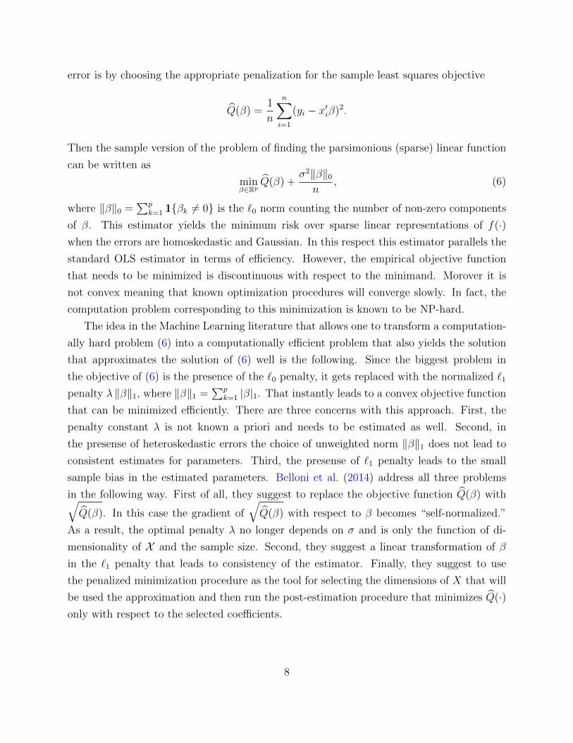
error is by choosing the appropriate penalization for the sample least squares objective

Q(β) =1

n

n∑i=1

(yi − x′iβ)2.

Then the sample version of the problem of finding the parsimonious (sparse) linear function

can be written as

minβ∈Rp

Q(β) +σ2‖β‖0

n, (6)

where ‖β‖0 =∑p

k=1 1{βk 6= 0} is the `0 norm counting the number of non-zero components

of β. This estimator yields the minimum risk over sparse linear representations of f(·)when the errors are homoskedastic and Gaussian. In this respect this estimator parallels the

standard OLS estimator in terms of efficiency. However, the empirical objective function

that needs to be minimized is discontinuous with respect to the minimand. Morover it is

not convex meaning that known optimization procedures will converge slowly. In fact, the

computation problem corresponding to this minimization is known to be NP-hard.

The idea in the Machine Learning literature that allows one to transform a computation-

ally hard problem (6) into a computationally efficient problem that also yields the solution

that approximates the solution of (6) well is the following. Since the biggest problem in

the objective of (6) is the presence of the `0 penalty, it gets replaced with the normalized `1

penalty λ ‖β‖1, where ‖β‖1 =∑p

k=1 |β|1. That instantly leads to a convex objective function

that can be minimized efficiently. There are three concerns with this approach. First, the

penalty constant λ is not known a priori and needs to be estimated as well. Second, in

the presense of heteroskedastic errors the choice of unweighted norm ‖β‖1 does not lead to

consistent estimates for parameters. Third, the presense of `1 penalty leads to the small

sample bias in the estimated parameters. Belloni et al. (2014) address all three problems

in the following way. First of all, they suggest to replace the objective function Q(β) with√Q(β). In this case the gradient of

√Q(β) with respect to β becomes “self-normalized.”

As a result, the optimal penalty λ no longer depends on σ and is only the function of di-

mensionality of X and the sample size. Second, they suggest a linear transformation of β

in the `1 penalty that leads to consistency of the estimator. Finally, they suggest to use

the penalized minimization procedure as the tool for selecting the dimensions of X that will

be used the approximation and then run the post-estimation procedure that minimizes Q(·)only with respect to the selected coefficients.

8

Formally, the minimization problem can be characterized as

β ∈ arg minβ∈Rp

1

n

n∑i=1

(yi − x′iβ)2 + λ‖Ψβ‖1, λ = 2√

2 log(pn)/n (7)

The optimal choice for the penalty constant in this case is λ = 2√

2 log(pn)n

, which means that

no additional steps are required to obtain its value. The transformation matrix Ψ resembles

the weights in the WLS procedure such that

Ψ = diag

√√√√ 1

n

n∑i=1

x2ijε

2i + op(1), j = 1, . . . , p

.

Provided that the residuals εi are not immediately available, they are replaced with the

estimates εi that are the outcome of the iterative procedure. The procedure initilizes at

εi = yi− y leading to Ψ = diag

(√1n

∑ni=1 x

2ij ε

2i +op(1), j = 1, . . . , p

). Then the we solve (7)

using Ψ as the transformation matrix yielding β. Then at the next step we use the updated

errors εi = yi − x′iβ to construct the new weighting matrix Ψ. The procedure iterates till

convergence. For the non-zero components of β we then run the regular OLS to find the

post-selection estimates.

3.2 SVM regression

Support vector machines (SVMs) are a class of estimators designed to solve the problem of

prediction of a discrete outcome using a vector of regressors X. We can easily illustrate the

idea behind the SVM approach for the settings where the outcome is determined by a linear

index of regressors. In other words the statistical model takes the form

Y = f(X) + ζ,

where f(X) =∑p

k=1wkXk + b = 〈w, X〉 + b and |ζ| ≤ ε. The problem as in LASSO is to

find a parsimonious set of relevant regressors in terms of their weights w. Allowing for the

error in the magnitude of at most ε, we can formulate the mathematical problem for finding

w from the sample {(yi, xi)}ni=1 as min ‖w‖2 subject to

yi − 〈w, xi〉 − b ≤ ε, and 〈w, xi〉+ b− yi ≤ ε.

9

Provided that the linear approximation may not exist for a given ε, Cortes and Vapnik (1995)

suggest introducing “slack” variables ξ and ξ∗ that transform the original problem into a

feasible problem:

min ‖w‖2 + Cn∑i=1

(ξi + ξ∗i )

subject to

yi − 〈w, xi〉 − b ≤ ε+ ξi, and 〈w, xi〉+ b− yi ≤ ε+ ξ∗i

for some constant C > 0 and non-negative slack variables ξ and ξ∗. The key idea in the

SVM is to construct the Lagrangian for the introduced constrained optimization problem and

replace the original optimization problem with the corresponding dual problem. Introducing

Lagrange multipliers α, α∗, η and η∗ we can write the Lagrangian as

L =1

2‖w‖2 + C

n∑i=1

(ξi + ξ∗i ) +n∑i=1

(ηiξi + η∗i ξ∗i ) +

n∑i=1

αi(ε+ ξi − yi + 〈w, xi〉+ b)

+n∑i=1

αi(ε+ ξ∗i + yi − 〈w, xi〉 − b).

The problem dual to the minimization of the Lagrangian with respect to the state variables

w, ξ, ξ∗ is the problem of maximization with respect to the co-state variables (Lagrange

multipliers) α, α∗, η, η∗. After simple re-arrangement this problem can be written as maxi-

mization of

−1

2

n∑i,j=1

(αi − α∗i )(αj − α∗j )〈xi, xj〉 − εn∑i=1

(αi + α∗i ) +n∑i=1

yi(αi − α∗i )

subject to∑n

i=1(αi−α∗i ) = 0 and 0 ≤ αi, α∗i ≤ C. This is the problem that can be efficiently

solved using quadratic programming. The observations i for which αi or α∗i are not equal to

zero are called the support vectors. The main insight from this formulation is that now the

estimated function of interest can be written as

f(x) =n∑i=1

(αi − α∗i )〈xi, x〉+ b.

This means that the impact of regressors x on the predicted outcome is summarized by the

inner product 〈·, ·〉. In the linear case the inner product is the standard inner product in the

Euclidean space.

10

Now suppose that X corresponds to some nonlinear transformation of a smaller set of

regressors Z. For instance, X can be different order polynomials of Z. In that case, the

inner product 〈xi, x〉 will also summarize the mapping Z 7→ X. This means that such an

inner product can be explicitly defined as a function of the original inputs z called the kernel

function. In this case the estimated regression function can be explicitly written in terms of

the kernel function

f(z) =n∑i=1

(αi − α∗i )k(zi, z) + b.

For a given function of two arguments to be a kernel it needs to be shown that it can be

represented as an inner product in some transformed space X (corresponding to Z 7→ X).

Several functions has been shown to be kernels and have been applied in practice. For

instance, the Gaussian function has been shown to be a kernel:

k(z, z′) = exp

(−‖z − z

′‖2

2σ2

).

Another example of the kernel is

k(z, z′) = B2r+1(‖z − z′‖),

where B2r+1 is the B-spline of order 2r + 1. The difference between the linear case (where

the function is estimated as a linear combination of inputs) and the case where the kernel

function is used is that the weights w are no longer defined explicitly. To give more intuition,

we can consider the case where the kernel can be written explicitly as k(z, z′) = 〈Φ(z), Φ(z′)〉.Then Φ(·) is the mapping that creates “regressors” X from Z. This will also allow to write

the weights as

w =n∑i=1

(αi − α∗i )Φ(xi).

We note that unlike LASSO, the regression SVM approach allows the space X to be explicitly

infinite-dimensional via the use of kernels.

3.3 L2 Boosting

Boosting algorithms are computationally fast methods that have been shown to have similar

properties to the LASSO methods in application to high-dimensional linear models. Al-

though initial applications of boosting were for the binary outcome variable, L2 boosting

11

with the associated quadratic loss function applies to the models with continuous outcome

variables. Unlike LASSO L2 boosting imposes an implicit penalty that is incorporated in

the structure of the algorithm itself. The algorithm is designed via the iterative verification

of the fit of the model over all of the dimensions of regressors. The algorithm then advances

along the dimension of the “best improvement,” i.e. the dimension where a given regressor

provides the biggest contribution to the least squares residual. The componentwise structure

eliminates the need to fit a high-dimensional least squares objective function replacing the

estimation with a series of one dimensional least squares procedures. Provided that at each

step one needs to verify the fit associated with each regressor in the model, it will be neces-

sary to compute p least squares minima. Due to the structure of the least squares objective

function the minimum can be written explicitly via the ratio of two sums further reducing

the computational burden.

The algorithm proceeds in four steps. First, the algorithm initializes at step m = 0 at

some f (0)(·) with the default value f (0)(·) = Y . Second, at step m+ 1 compute the residuals

ε(m)i = yi − f (m)(xi).

The model is then fitted using a componentwise linear least squares. (i) Compute the

coefficients

γ(m)j =

∑ni=1 xij ε

(m)i∑n

i=1(xij)2.

(ii) Find the dimension to be updated j(m) = arg minj≤p∑n

i=1

(ε

(m)i − γ(m)

j xij

)2

. (iii) Up-

date the estimated coefficients as f (m+1)(x) = f (m)(x) + ν γ(m)

j(m)xj(m) . The choice of the

step-length factor ν does not impact the asymptotic behavior of the algorithm and is usu-

ally selected to be “sufficiently small” (e.g. ν = 0.1). The componentwise linear least

squares thus updates only one dimension of the model at a time. Finally, the second step

is iterated until the stopping iteration M has been reached. The recommended choice is

M = K(√

n/ log(p))(3−δ)/(4−2δ)

for 0 < K <∞ and 0 < δ < 5/8.

4 Econometric properties of averaged models

Above we discussed three Machine Learning methods. We note that the main difference

between the SVM regression, L2 boosting and square-root LASSO is that the SVM regression

does not explicitly use the “generated features” x = Φ(z). Instead, the (large) vector of

12

generated features is embedded in the kernel function. Our goal is to ensure that the three

discussed methods have adequate performance when evaluated in the average model. That

would in general require that each of the estimators attains the convergence rate of o(n−1/4).

That would allow us to use existing results regarding the performance of average predictions

and establish asymptotic normality and O(n−1/2) convergence rate for the corresponding

average predictor.

There are three sets of conditions that need to be imposed on the econometric model

to ensure the adequate performance of the resulting estimator. First, we need to ensure

that the distributions of regressors and the unobserved disturbances a sufficiently regular

so that the concentration inequalities leading to limit theorems can be applied. Second, we

need to verify that the sequence of functional spaces that we use to approximate the non-

parametric model provides sufficiently good approximation. The properties of approximating

functional spaces used for semi- and non-parametric inference have been extensively studied

in econometrics, e.g. including Andrews (1991), Newey (1997) and Chen (2007). Finally, we

need to impose the constraint on the complexity of the approximating model such that it

appropriately trades off the approximation and the estimation errors.

We start with the imposition of properties on the statistical components of the model.

ASSUMPTION 1 Suppose that the higher order maximum and minimum moments of

regressors and disturbances satisfy the following conditions.

(i) For q > 4, 1n

∑ni=1E[|εi|q] <∞

(ii) infn≥1 min1≤j≤p1n

∑ni=1 P

pj(zi)2E[ε2i ] > 0 and supn≥1 max1≤j≤p

1n

∑ni=1 |P pj(zi)|3E[|εi|3] >

0, where P pj(·) are basis functions of the approximating space described in the next as-

sumption.

Next we impose a high-level condition on the approximating functional space and the

corresponding estimator. The estimator itself will need to be appropriately selected, e.g.

using the guidelines in Chen (2007) and will depend on the underlying properties of the

function that is approximated (such as smoothness, monotonicity, etc.).

ASSUMPTION 2 Suppose that

(i) f(·) ∈ F is an element of a compact subset of separable Hilbert space H and there is a

sequence of finite-dimensional vector spaces Hp such that Hp ⊂ Hp+1 ⊂ H and there is

a sequence of orthogonal bases {P pk(·)}pk=0 such that Hp is a completion of the linear

span of {P pk(·)}pk=0.

13

(ii) For each n and for any f ∈ F and any p� n there exists a subsequence {P pkj(·)}sj=1

with s� p such that the class of functionsRp ={rp(·) = f(·)− proj

(f | {P pkj(·)}sj=1

), f ∈ F

}has a finite envelope Rp with

E[(Rp)2] ≤ C s log(p)/n

(iii) The inner product in each Hp and and an element Φp(·) of Hp generate a kernel

Kp(·, ·) = 〈Φp, Φp〉Hp ≤ Kp such that

proj(f | {P pkj(·)}sj=1

)= 〈w, Φp〉Hp ,

for w ∈ Hp and ‖w‖Hp < Λ <∞

Assumption 2 essentially specifies the properties of the feature map that approximates the

nonparametric regression. Associated with this feature map is the corresponding kernel

defined as an inner product in Hp.

Finally, we provide the set of assumptions that ensure the appropriate tradeoff between

the sample size and the complexity of the approximating functional space.

ASSUMPTION 3 Let ∆p be the subspace of Rp such that 0 6∈ ∆p and for each δ ∈ ∆p

the component δkj > 0 where 0 < kj ≤ p is the subsequence defined in Assumption 2

and δk = 0 otherwise. Let ln → ∞. Define λn = minδ∈∆p,‖δ‖0≤sln

δ′( 1n

∑ni=1 P

p(zi)iPp(zi)

′)δ(δ′δ)1/2

and

λn = maxδ∈∆p,‖δ‖0≤sln

δ′( 1n

∑ni=1 P

p(zi)iPp(zi)

′)δ(δ′δ)1/2

. Suppose that

(i) supn≥1

λnλn<∞.

(ii) maxi≤n,j≤p |P pj(zi)|2/ln = o(1), log p ≤ C(n/ log2 n)1/3 and l2ns log(p) ≤ Cn/log n.

(iii) Kp → 0 as p→∞ and Kp√n→∞

Based on Assumption 2, we can integrate the results in Belloni et al. (2014), Cortes and

Vapnik (1995) and Meinshausen and Buhlmann (2006) to provide the following theorem.

THEOREM 1 Suppose that statistical model satisfies Assumptions 1, 2, and 3. Consider

the√

LASSO algorithm with λ = 2√

2 log(pn)/n, the SVM regression algorithm with ε =

14

o (Kp√n) and C ≥ E[(Rp)2]1/2, and the L2 boosting algorithm with M = O

((√n/ log(p)

)(3−δ)/(4−2δ))

with 0 < δ < 5/8. Then for each resulting estimator

1√n

n∑i=1

(f(zi)− f(zi))2 = op(1).

The property of the constructed estimator allows us to apply it in the settings of model

averaging. The object of interest is the average prediction with the weighing function w(·)such that the final parameter of interest can be expressed as

θ = E[w(Z)f(Z)]. (8)

Our next idea is to apply the result in Newey (1994) which assures that as long as model

(8) is written in the “orthogonal form” with respect to the nonparametrically estimated

function f(·) then the particular estimator of f(·) will not have an impact on the asymptotic

distribution and thus the implementation details of the machine learning methods that we

used to estimate f(·) will not affect the resulting average prediction.

THEOREM 2 Suppose that f(·) is a machine learning method satisfying conditions of

Theorem 1 and (8) along with the data generating process satisfy Assumptions 5.1-5.3 in

Newey (1994). Then the resulting average prediction θ is asymptotically normal with

√n(θ − θ) d−→ N(0, V )

with

V = Var(Ψ(Y, Z)) = E[w(Z)2σ2(Y |Z)] + Var(w(Z)f(Z))

Proof:

Suppose as before that z ∈ Z ⊂ Rd with d � n and finite. Consider the likelihood of

the model `(y, z) and consider its parametrization `t(y, z) with some scalar parameter t.

Denote st(y|z) the score of the conditional distribution `t(y|z) and st(z) the score of the

unconditional distribution `t(z). The full score st(y, z) = st(y|z) + st(z). Then we can

write the tangent space of the model Tt = {a(y, z) + t(z)} where E[a(Y, Z)2] < ∞ and

E[a(Y, Z)|Z = z] = 0 and E[t(Z)2] < ∞ and E[t(Z)] = 0. Now we consider the sequence

of parameters θt corresponding to the sequence of distributions `t(y, z) and consider the

directional derivative∂θt∂t

=∂

∂tEt[w(Z)ft(Z)].

15

We can express this derivative using the fact that ft(z) = Et[Y |Z = z]:

∂θt∂t

= E[w(Z)f(Z)st(Z) + w(Z)Y st(Y |Z)].

Now the idea to find the “orthogonal” form of the estimator will be to find an element of

Tt such that the directional derivative of the parameter of interest can be represented as a

projection of the score of the parametrized model on the tangent space. A straightforward

verification suggests that∂θt∂t

= E[Ψ(Y, Z)st(Y, Z)],

where

Ψ(y, z) = w(z)(y − f(z)) + (w(z)f(z)− E[w(Z)f(Z)]).

Next we apply Lemma 5.3 in Newey (1994) to the estimator defined by

θ − E[w(z)f(Z)] =1

n

n∑i=1

Ψ(yi, zi)

with f(·) replaced with f(·). Provided that the estimator f(·) satisfies assumptions of The-

orem 1 is satisfies conditions of Lemma 5.3 in Newey (1994). This leads to the result that

√n(θ − θ) d−→ N(0, V )

with

V = Var(Ψ(Y, Z)) = E[w(Z)2σ2(Y |Z)] + Var(w(Z)f(Z))

Q.E.D.

5 Additional empirical procedures

In addition to the three inference procedures described above we consider four additional

machine learning procedures that we also interpret as methods for the estimation of the

conditional expectation E[Y |Z = z].

16

5.1 Forward stepwise and forward stagewise models

As in the square-root LASSO procedure and L2 boosting we consider an explicit mapping

Z 7→ X . As in standard nonparametric models this mapping can be represented via a

collection of basis functions {P pj(·)}pj=1 where the size of the set of functions p is allowed to

slowly grow with the sample size n. Unlike LASSO, where the model is selected by fitting

the penalized least squares objective function that leads to corner solutions making multiple

coefficients to be equal to zero, the stepwise and stagewise models lead to sparse coefficient

sets via the construction of the variable selection procedure.

The incremental version of the stagewise regression model uses the explicitly set step size

ε that can be calibrated based on the convergence performance of the estimation procedure.

The procedure itself is based on the iterative addition of the “explanatory variables” P pj(·).The procedure is initialized from the baseline model f (0)(z) = y with the corresponding coef-

ficients of the nonparametric representation β(0)j ≡ 0. The corresponding residuals are com-

puted in the standard way as r(0)i = yi−f(zi). Then at iteration k we find the predictor P jp(·)

maximizing the correlation between r(k)i and P jp(zi). Then the corresponding coefficient in

the nonparametric representation is updated as β(k+1) = β(k) + ε sign(corr(r(k), P pj(·))

).

The residual then is updated to offset the change in the coefficient βj. The procedure then

stops when the maximum correlation between r(k)i and P jp(zi) does not exceed the pre-set

tolerance (or the maximum allowed number of steps has been achieved). In our analysis we

choose the maximum number of steps at 16,000 to ensure that the procedure is stopped via

the tolerance criterion.

In the stepwise algorithm, the set of regressors used for estimation is iteratively updated

based on the minimization of the Akaike Information Criterion. The model is initialized

at f (0)(z) = y same as in the stagewise method. Then at step k we select one of the

components P jp(·) for which β(k−1)j = 0 that yields the highest contribution to the AIC. This

re-computation can be done efficiently by invoking the QR factorization in the corresponding

first order condition and thus does not require a repetitive multi-dimensional minimization.

The procedure stops once the improvement in the AIC falls below the selected tolerance or

the maximum set number of steps is exceed.

5.2 Regression Trees and the Random Forest

The random forest model is different from most of the models that we considered previously

in the sense that it is explicitly not using the spectral properties of the functional space that

17

contains f(z) = E[Y |Z = z]. Instead, the method is based on selecting the best iterative

factorization of the state space Z such that within each element of the partition of the state

space function f(·) can be approximated by a constant.

The basic element of the random forest algorithm is a regression tree. The regression tree

is defined by two basic parameters: the maximum depth (also called the number of splits)

and the size of the terminal nodes (also called leaves) determining the minimum number of

points within each partition of the state space. Denote the tree parameters θ. Then given the

sample Zn = {z}ni=1 the regression tree is defined by the following algorithm. The algorithm

is initialized at f (0)(z) = y. At step k the state space is split into rectangular areas R(k)j and

the regression tree predicts as

f (k)(z) =∑j

∑ni=1 yi1{zi ∈ R

(k)j }∑n

i=1 1{zi ∈ R(k)j }

1{z ∈ R(k)j }.

Then the algorithm is updated by searching for the partition element R(k)j and the dimension

l of z such that if R(k)j = [z1

jL, z1jU ]× . . .× [zpjL, z

pjU ], then the split of this partitions into two

R(k+1)j1

= [z1jL, z

1jU ]× . . .× [zljL, 0.5(zljU + zljU)]× . . .× [zpjL, z

pjU ] and R

(k+1)j2

= [z1jL, z

1jU ]× . . .×

[0.5(zljU +zljU), zljU ]× . . .× [zpjL, zpjU ] provides the greatest contribution to the sum of squared

residuals corresponding to the new partition Rk+1)j :

minl=1,...,p, R

(k)j

n∑i=1

(yi − f (k+1)(zi))

over all j and dimensions l = 1, . . . , p. The iterations continue until one of the convergence

criteria (the size of the terminal node or the depth of the tree) is met. It can be shown that

when the outcome variable is binary, the minimization problem used to construct the tree is

analogous to Manski’s maximum score problem over the binary splits of the state space.

The random forest model is generated as an ensemble of trees via bootstrap. One draws

B bootstrap samples from the original sample Xn. Each such a bootstrap sample Xb and

the corresponding parameters θb yield the estimated regression tree fb(·). Then the random

forest model provides the value which is the average over the bootstrap samples:

f(z) =1

B

B∑b=1

fb(z).

18

6 Empirical Application

This section compares econometric models with machine learning ones using a typical de-

mand estimation scenario—grocery store sales. The machine learning models in general

produce better out-of-sample fits than linear models without loss of in-sample goodness of

fit. If we combine all the models linearly with non-negative weights, the resulting combina-

tion of models produces better out-of-sample fit than any model in the combination. This

section also illustrates how machine learning models could work with unstructured data or

sparse data. Unstructured data is not organized to feed into models directly like structured

data. For instance, the text description of a bag of chips and the image of the bag are

unstructured data. Sparse data is a type of data where most of the elements are zeros. Both

of unstructured and sparse data would be hard to handle in econometric models. The last

part of this section uses the same data and model structures to estimate the promotional lift

of sales.

The data we use is provided by IRI Marketing Research via an academic license at the

University of Chicago. It contains scanner panel data from grocery stores within one grocery

store chain for six years. We used sales data on salty snacks, which is one of the categories

in the IRI data. A unit of observation is product j, uniquely defined by a UPC (Universal

Product Code), in store m at week t. There are 3,045,513 observations, which includes 3,337

unique products. Let qjmt be the number of bags of salty snack j sold in store m at week t. If

qjmt = 0, we do not know if it is due to no sale or out-of-stock and the observation is not filled

in. The price pjmt is defined as the quantity weighted average of prices for product j in store

m at week t. Therefore if qjmt = 0, the weight is also 0. In addition to price and quantity, the

data contains attributes of the products (such as brand, volume, flavor, cut type, cooking

method, package size, fat and salt levels) and promotional variables (promotion, display

and feature). Table 1 shows the summary statistics of quantity, price and dollar spent per

transaction. Table 2 shows the number of unique values for the category variables as well

as the three most common values of product attributes: brand, volume, flavor, cut type,

cooking method, package size, fat and salt levels.

In our application, we compare eight alternative models of demand to predict qjmt. The

eight models are linear model, stepwise, forward stagewise, LASSO, random forest, support

vector machine, gradient boosting trees, and Logit. Linear model and Logit are traditional

econometric models where the others are popular machine learning algorithms. We also

perform a linear combination of all the models in the effort to increase prediction accuracy.

We use R to compute all the results and a list of related R packages is provided in this

19

Table 1: Summary Statistics

Variable Mean Median

Price 2.12 1.99Quantity 15.80 6.00Dollars 28.11 12.19

#Stores 1,560#Weeks 313#UPC 3,337#Obs 3,045,513

Table 2: Category Variables

Variable #Levels Three Most Frequent Values

Brand 237 Pringles Utz LaysProduct Type 4 Potato Chip Potato Crisp Potato Chip and DipPackaging 20 Bag Canister Plastic Wrapped Cardboard CanisterFlavor 207 Original Sour Cream & Onion BBQFat Content 16 Missing Low Fat Fat FreeCooking Method 47 Missing Kettle Cooked Old Fashion Kettle CookedSalt Content 14 Missing Lightly Salted Sea SaltCutting Type 32 Flat Missing Ripple

section.

6.1 Linear Regression Models

The linear regression is a typical approach to estimate demand by approximating the demand

using a function form of the following:

ln qjmt = β′Xjmt + ζmt + ηjm + εjmt

where Xjmt is the matrix of attributes including log of own prices, product attributes, adver-

tising and promotion indicators, ζmt is the market specific seasonal factor, ηjm is the product

specific market effect and εjmt is an idiosyncratic shock to each product, market and time.

Table 3 shows the output of the linear model where only the significant coefficients are

displayed.

20

Table 3: Linear Regression

Log Quantity Estimate Std. Error t value Pr(> |t|)

Log Price -0.639 0.055 -11.708 < 2e-16 ***Promotion 0.466 0.039 11.926 < 2e-16 ***Feature: None -0.630 0.067 -9.334 < 2e-16 ***Display:Minor 0.708 0.049 14.341 < 2e-16 ***Major 0.637 0.049 13.119 < 2e-16 ***Brand:Herrs -0.351 0.156 -2.253 0.024 *Jays -1.101 0.244 -4.516 0.000 ***Kettle Chips -0.995 0.236 -4.217 0.000 ***Lays -0.337 0.159 -2.124 0.034 *Lays Bistro Gourmet -0.656 0.188 -3.480 0.001 ***Lays Natural -1.662 0.327 -5.079 0.000 ***Lays Stax -1.481 0.183 -8.104 0.000 ***Lays Wow -0.485 0.204 -2.379 0.017 *Michael Seasons -1.655 0.239 -6.921 0.000 ***Pringles -0.794 0.156 -5.090 0.000 ***Pringles Cheezums -0.644 0.211 -3.055 0.002 **Pringles Fat Free -0.624 0.189 -3.308 0.001 ***Pringles Prints -1.876 0.314 -5.982 0.000 ***Pringles Right Crisps -0.881 0.128 -6.892 0.000 ***Ruffles Natural -1.379 0.389 -3.549 0.000 ***Ruffles Snack Kit -1.555 0.307 -5.061 0.000 ***Utz -0.543 0.149 -3.635 0.000 ***Wise -0.505 0.165 -3.062 0.002 **Wise Ridgies -0.984 0.167 -5.888 0.000 ***Volume 0.469 0.113 4.142 0.000 ***Package:Canister 0.437 0.091 4.800 0.000 ***Canister In Box 0.453 0.130 3.494 0.000 ***Flavor:BBQ 0.167 0.066 2.534 0.011 *Cheddar 0.241 0.080 3.026 0.002 **Cheese -0.443 0.205 -2.164 0.031 *Ketchup -0.680 0.244 -2.787 0.005 **Onion 0.339 0.066 5.107 0.000 ***Original 0.704 0.061 11.588 < 2e-16 ***Spicy -0.211 0.105 -2.005 0.045 *Salt: No Salt -0.446 0.212 -2.099 0.036 *Type of Cut: Flat 0.308 0.070 4.411 0.000 ***Store Fixed Effects YesWeek Fixed Effects Yes

Adjusted R-squared 0.884Significance 0 *** 0.001 ** 0.01 * 0.05 .

21

Table 4: Logit with Regression Selection

Log Share Estimate Std. Error t value Pr(> |t|)

Log Price 0.296 0.113 2.624 0.009 **Promotion -0.441 5.192 -0.085 0.932Feature: None 0.263 0.151 1.745 0.081 .Display:Minor -0.215 0.104 -2.080 0.038 *Major -0.338 0.113 -3.000 0.003 **Store Fixed Effects NoWeek Fixed Effects No

AIC 6884.4Significance 0 *** 0.001 ** 0.01 * 0.05 .

6.2 Logit

We followed Berry et al. (1995) to do a logit-type model of market shares. We project

estimated qjmt on product attributes dummies, store fixed effects and week fixed effects.

Then we sum qjmt over stores and weeks. Assuming that market sizes are fixed, we calculate

market share by dividing qjmt by market size. The log of market share is taken as the

dependent variable in our Logit model. Table 4 shows the output of Logit model with

traditional regression where only the significant coefficients are displayed.

6.3 Stepwise, Forward Stagewise and Sqrt LASSO

In practice, stepwise and forward stagewise can be realized in R package lars. We take the

default parameter t and λ in the package. These three model converge in similar ways

where in each step, the most important variable is added to the model. We limit the

maximum number of steps to 100 in our practice for demonstration purposes because it

takes significantly longer to converge if the number of steps is larger.

Square Root Lasso is from the slim function of R package flare, where slim stands

for Sparse Linear Regression using Non-smooth Loss Functions and L1 Regularization. In

function slim, we set type=lq and q=2 (loss function) to use the Square Root Lasso. Default

number of lambdas in the sequence is 5. We set it to be 40. Default min/max value of the

sequence of lambdas is 0.3*max and π√

(log(d)/n). The authors of the flare package stated

that SQRT Lasso is tuning insensitive based on Belloni et al. (2011).

22

Table 5: Random Forest Variable Importance

Log Quantity%Increase in Mean

Squared ErrorIncrease in Node Purity

Log Price 74.83 1196.68Volume 56.81 855.79Display: Minor 49.79 455.98Promotion 43.76 519.72Display: Major 43.29 267.43Feature: None 42.05 592.37Brand: Lays 39.82 367.29Brand: Ruffles 33.21 76.97Brand: Wavy Lays 32.95 143.46Flavor: Classic 32.31 219.00Flavor: Sour Cream & Onion 30.26 62.28

R-Squared 0.42

6.4 Random Forest

Random forecast is implemented in R package randomForest. Random forest has a few

parameters about the tree structure: mtry as the number of variables to randomly select at

each tree, ntree as the number of trees in the model, nodesize as the minimum size of the

terminal nodes of each tree, and maxnodes as the maximum number of terminal nodes each

tree can have.

We first run a cross-validated version of random forest (function rfcv) to determine the

best number of variables to sample at each tree. This function uses K-fold cross-validation.

We set scale=log, step=0.5, which means we will drop 50% of the variables in every step.After

we determine the best number of variables to try at each tree, a random forest model

(function randomForest) was executed with the optimal mtry and the other parameters

at default values. The default value for nodesize is 5, ntree 500 and maxnodes NULL. The

cross-validation function rfcv does not decide the optimal values for these parameters.

Table 5 displays the variable importance of the twelve most important variables in de-

termining Log Quantity using two metrics. The percentage increase in mean squared error

is the increased percentage of mean squared error if a variable is excluded from the model.

Node purity measures how much the additional variable or tree split reduces the residual

sum of squares. Thus, the increase in node purity measures the size change in node purity

if a variable is excluded from the model.

23

6.5 Support Vector Machine

We use functions svm and tune.svm in R package e1071 to implement the support vector

machine model. We specify type=eps-regression as our dependent variable continuous.We

specify a 10-fold cross-validation in the support vector machine.

We use a tuning function tune.svm to do the 10-fold cross-validation of SVM to determine

the best parameters of epsilon, cost and gamma. Epsilon is ε in the loss function with default

0.1. We test epsilon from 0 to 1 with interval 0.2. Cost is the constant of the regularization

term in the Lagrange formulation. We test cost from 0.5 to 2 with interval 0.5. Gamma

is the parameter in the kernel function. We test gamma from 0.01 to 0.1 with length of

five. The kernel used in the training is radial basis - Gaussian. This is tested in our data to

out perform the other kernels. The other kernel options are polynomial, linear and sigmoid.

Here are the kernel functions:

• linear: u′v

• polynomial: (γu′v + coef0)degree

• radial basis: exp(−γ|u− v|2)

• sigmoid: tanh(γu′v + coef0)

6.6 L2 Boost

L2 Boost is from function glmoost of R package mboost for boosting with component-wise

least squares. We define the loss function as the squares of errors and define the negative

gradient and stopping parameter for the glmoost function.

Table 6 shows the coefficients from L2 Boost where only 36 out of 2243 variables have

non-zero coefficients (we show only a portion of the non-zero coefficients).

6.7 Combined Model

In order to compare models, we want to split the data into training and testing set, where

we train the model using the training set and pretend the dependent variable in the test set

is unknown and predict on the test set. Because we have eight models, we want to assign

weight to each model when building a linear combination. However, the weight based on the

training set is biased. Some models like linear model tend to get a good in-sample fit but a

24

Table 6: L2 Boost Coefficients

Log Quantity Coefficient

Log Price -19.57Promotion 18.24Feature: Medium Ad 4.79Feature: None -19.85Display: Minor 12.78Display: Major 18.88Brand: Kettle Chips -3.41Brand: Lance Thunder -0.48Brand: Lays 16.50Brand: Lays Stax -2.30Brand: Ruffles 6.26Brand: Wavy Lays 10.06Flavor: Classic 11.30Flavor: Sea Salt & Vinegar -0.45Type: Potato Chip and Dip -0.49Type: Potato Crisp -1.10Package: Canister in Box -4.08. . .

bad out-of-sample fit, and this grants these model a very large in-sample weight which could

be misleading.

Therefore, we randomly split the data into three pieces to do cross validation, where

the model weights are determined on the validating set. This three way data partitioning

mitigates the possible large out-of-sample error for some models when over fitting happens.

25% of the data is used as the test set, 15% is used as the validate set, and the remaining

60% is used as the training set. Table 8 shows how the data is sliced into three pieces.

6.7.1 Combining Models with Asymptotic Properties

We combine six models that has asymptotic properties using a constrained linear regression,

in Table 7. The six models are: linear regression, Square-root Lasso, Support Vector Ma-

chine, L2 Boosting, Logit with market share predicted by a regression model. The response

variable is log of quantity sold per week. The covariates are log of price, product attributes

variables, promotional variables, store fixed effects, and week fixed effects. We provide the

same covariate matrix to all of the models expect for the Logit model, where all the fixed

effects are excluded.

We combine them using the following algorithm:

1. Fit the actual dependent variable in the training set on each of the five models.

25

Table 7: Linear Model Combination: Models with Asymptotics

Train Validation Test

RMSE Std. Err. RMSE Std. Err. RMSE Std. Err. Weight

Linear 0.766 0.010 0.994 0.017 1.010 0.015 10.41%Sqrt Lasso 0.977 0.007 0.984 0.013 0.995 0.009 1.71%Support Vector Machine 0.543 0.007 0.889 0.018 0.900 0.012 87.57%L2 Boosting 1.053 0.004 1.016 0.013 1.028 0.012 0.00%Logit 3.282 0.170 3.509 0.340 3.915 0.263 0.32%

Linearly Combined 0.887 0.898 100.00%

# of Obs 1,827,308 456,827 761,379Total Obs 3,045,513% of Total 60% 15% 25%

2. Make out-of-sample prediction using the model coefficients from the first step on the

validate set.

3. Take only the validation set. Treat the predicted values of the dependent variable from

the five models as regressors, treat the actual value of the dependent variable as the

response variable, then do a constrained linear regression. The sum of the coefficients

are constrained to be one. Get all the coefficients and regard them as weights in the

combined model.

4. Use the fitted models to predict in the test set, and apply the weights from validate

set to each model, sum them up and form the linearly combined prediction.

In Table 7, support vector machine gets the most weight out of the five models due to

its small prediction error (measured by RMSE) in the validation set. Its prediction error in

the test set is also the smallest among all models.

6.7.2 Combining All Models

In Table 8, we compare eight models: two of them are traditional econometrics models and

seven of them are more in the context of machine learning as introduced before. Our purpose

is to run a horse race of models by comparing out-of-sample prediction errors.

Table 8 shows the comparison of the models. In the scenario of out-of-sample prediction

error, the best two models are random forest and support vector machine. The combined

model, where we regress the actual value of the response variable on a constrained linear

model of the predictions from eight models, outperforms all the eight models, which follows

26

Table 8: Model Comparison: Prediction Error

Train Validation Test

RMSE Std. Err. RMSE Std. Err. RMSE Std. Err. Weight

Linear 0.766 0.010 0.994 0.017 1.010 0.015 17.73%Stepwise 0.930 0.008 0.969 0.017 0.980 0.014 0.00%Forward Stagewise 0.977 0.007 0.985 0.015 0.995 0.013 0.00%Sqrt Lasso 0.977 0.007 0.984 0.013 0.995 0.009 0.00%Random Forest 0.927 0.007 0.914 0.017 0.916 0.013 37.46%Support Vector Machine 0.543 0.007 0.889 0.018 0.900 0.012 44.79%L2 Boosting 1.053 0.004 1.016 0.013 1.028 0.012 0.00%Logit 3.282 0.170 3.509 0.340 3.915 0.263 0.02%

Linearly Combined 0.879 0.887 100.00%

# of Obs 1,827,308 456,827 761,378Total Obs 3,045,513% of Total 60% 15% 25%

the optimal combination of forecasts in Bates and Granger (1969). Random forest and sup-

port vector machine get more weights in the combined model due to their good performance

out-of-sample.

Based on Section 3, the combination of models converges to asymptotic normal distri-

bution at√n rate, regardless of the what individual models there are. Therefore, we could

bootstrap the combined model to get the confidence interval, knowing that it is asymptoti-

cally normal.

Table 9 provides the summary statistics of the residual between predicted and actual

values of quantity in both validation and testing set.

6.8 Asymptotics

We dedicate this section to show empirically the asymptotics of the selected machine learning

models mentioned in Section 3. We use our dataset but limit the number of observations to

a sequence of smaller numbers. We run the same model specification as the main application

for these datasets of different sizes and compute standard errors of the root mean square

error in prediction using subsampling. As Table 10 Figure 1 shows, in both validate and test

set, the standard errors are going to zero when the number of observation grows.

27

Table 9: Summary Statistics of Residual in Prediction

Validation Set Mean Std. Dev. Median Min Max

Linear -0.019 1.549 -0.015 -5.402 4.862Stepwise -0.023 1.440 0.018 -4.942 4.365Stagewise -0.023 1.353 0.040 -4.549 3.975Sqrt Lasso -0.023 1.347 0.011 -5.501 4.035Random Forest 0.010 1.424 0.073 -4.591 4.618Support Vector Machine -0.010 1.462 0.008 -4.387 5.167L2 Boost -0.024 1.399 0.025 -4.952 4.661Logit -0.244 3.566 0.154 -39.141 3.135Combined -0.004 1.466 0.028 -4.811 5.053

Test Set Mean Std. Dev. Median Min Max

Linear -0.012 1.533 0.013 -5.385 5.387Stepwise -0.029 1.429 -0.026 -5.568 4.726Stagewise -0.072 1.402 -0.073 -4.521 3.869sqrt Lasso -0.056 1.375 -0.066 -6.262 4.069Random Forest 0.088 1.489 0.168 -5.912 4.802Support Vector Machine 0.004 1.515 0.012 -5.771 5.430L2 Boost -0.080 1.462 -0.031 -5.888 4.379Logit -0.322 3.910 0.154 -38.241 2.833Combined -0.033 1.435 -0.038 -5.126 4.698

Table 10: Convergence Rate for Three Machine Learning Models

Sample Size 100 200 400 800 1600 3200 6400 12800

Validate

Sqrt Lasso 0.2025 0.1380 0.0909 0.0566 0.0382 0.0320 0.0225 0.0162Support Vector Machine 0.1613 0.1180 0.0767 0.0446 0.0375 0.0222 0.0162 0.0137L2 Boosting 0.0487 0.0788 0.0467 0.0325 0.0318 0.0223 0.0177 0.0133Combined 0.1944 0.1468 0.0828 0.0574 0.0417 0.0316 0.0258 0.0159

Test

Sqrt Lasso 0.2125 0.1364 0.0790 0.0492 0.0292 0.0259 0.0170 0.0130Support Vector Machine 0.1635 0.1245 0.0765 0.0435 0.0299 0.0186 0.0142 0.0099L2 Boosting 0.0621 0.0786 0.0466 0.0313 0.0261 0.0185 0.0138 0.0099Combined 0.2251 0.1476 0.0813 0.0519 0.0367 0.0258 0.0199 0.0136

28

Figure 1: Standard Errors of RMSE

validate

test

0.00

0.05

0.10

0.15

0.20

0.00

0.05

0.10

0.15

0.20

400800 1600 3200 6400 12800

Obs

Sta

ndar

d E

rror

s

model L2Boosting sqrtLasso SVM

6.9 Discussion

6.9.1 Variable Selection

When the number of independent variables is large, it is common to have some degree of

multicollinearity. The shrinkage models could help us reduce the multicollinearity intelli-

gently. A usual statistics to determine multicollinearity is Variance Inflation Factors (VIF).

The VIF for covariate Xj is defined as:

V IFj =1

1−R2−j

(9)

where R2−j is the R-squared by regressing covariate Xj on the rest of covariates. Table 11

shows some VIFs for the independent variables used in the linear regression model. To

compare, after LASSO selects variable, we also have the VIFs for the independent variables

in the linear regression using only selected variables. The VIFs in the non-selecting case

are much higher than the LASSO selection for many variables. Using 5 as a threshold for

multicollinearity, LASSO successfully reduces multicollinearity in the independent variables.

29

Table 11: Variance Inflation Factors

VIFs after Selection

Variable Linear LASSO

Product Type - Potato Chip And Dip +∞ 3.5084Brand - Ruffles Snack Kit +∞ 3.4729Logprice 4.1750 3.2319Volumn 3.9775 3.1541Cooking - Missing +∞ 3.1100Cooking - Kettle +∞ 2.6495Package - Canister +∞ 1.8047Fat - Regular 76.6610 1.5930Brand - Lays 104.5904 1.5187Promotion 1.4806 1.4388Feature - None 2.3398 1.3369Brand - Kettle Chips 27.3608 1.3222Flavor - Original 2.8610 1.2875Brand - Ruffles 50.1427 1.2802Salt - Regular 3.0660 1.2732...

We believe it’s more attractive than ad hoc variable selection procedures commonly used in

practice.

6.9.2 Random forest on the individual model pieces

We use the predicted values of all the eight models from the validation set as input variables

and use the actual log quantity as the output variable to train the random forest model. We

do a 10-fold cross-validated version of random forest to determine the best parameters (same

approach as described in Section 6.4) and then predict the output variable log quantity in

the test set. Then we evaluate the prediction by the combined model with RMSE.

Table 12 shows combining the eight models using a random forest model instead of linear

combination in Table 8. The importance of each individual model is shown in the right

column, which is similar to the Weight column of Table 8.

6.9.3 Bag of Words (XXX: move up to main text)

The mere feat of encoding a vector of hedonic attributes commonly used in demand esti-

mation for this data could be cumbersome. In applied econometrics, researchers commonly

restrict attention to the products with the largest demand and encode regressors for brands

and a small vector of product attributes. In our application, we propose using unsupervised

30

Table 12: Combining Models in Random Forest

Train Validation Test

RMSE Std. Err. RMSE Std. Err. RMSE Std. Err. Var. Imp.

Linear 0.766 0.010 0.994 0.017 1.010 0.015 32.435Stepwise 0.930 0.008 0.969 0.017 0.980 0.014 32.647Forward Stagewise 0.977 0.007 0.985 0.015 0.995 0.013 24.607Sqrt Lasso 0.977 0.007 0.984 0.013 0.995 0.009 23.135Random Forest 0.927 0.007 0.914 0.017 0.916 0.013 34.845Support Vector Machine 0.543 0.007 0.889 0.018 0.900 0.012 52.972L2 Boosting 1.053 0.004 1.016 0.013 1.028 0.012 23.977Logit 3.282 0.170 3.509 0.340 3.915 0.263 0.932

Combined by Random Forest 0.920 0.902

# of Obs 1,827,308 456,827 761,378Total Obs 3,045,513% of Total 60% 15% 25%

Note: In random forest, variable importance is defined as the average difference in out-of-bag mean squared errorwith and without permuting the variable, divided by the standard deviation of the difference. The bigger thevariable importance value, the more important the variable is.

learning to construct product level regressors. In particular, we use the unstructured text

that describes the product in the raw data and apply the bag of words model. This has

the advantage of being a simpler computation and allows us to avoid the arduous task of

encoding attributes for thousands of products. Since it is more scalable, it allows us to

model the demand for all of the products rather than restricting attention to the products

with the largest demand. Also, it could be viewed as less ad hoc than hand coding product

attributes since it imposes fewer a priori restrictions on the hedonic attributes that we should

include as regressors in our model. We note that there is a large literature on this form of

unsupervised learning which sometimes goes by the name of feature extraction in computer

science. With the exception of Gentzkow and Shapiro (2010), there has been relatively little

use of this method in economics. We believe that this is promising for demand estimation

because it allows a new source of data to construct covariates such as the raw text in product

descriptions or product reviews.

Aside from structured features like package type, cut type of potato chips, the hedonic

attributes of the product can also be defined by unstructured texts that describe the product.

A bag of words model could easily turn the unstructured texts into large amounts of features.

Unsupervised learning (clustering) on these features could be a more scalable approach than

hand coding them. The procedures following the unsupervised learning are the same as

the way we deal with structured features. Yet this straightforward approach has better

31

prediction power than structured models.

The bag of words model analyzes a corpus of K documents, comprising a dictionary of

M words, and finds the relations of words and documents. In our case, the K documents are

the n unique potato chips descriptions. We cluster the descriptions, via manipulation of the

document-term matrix. A document-term matrix is a mathematical matrix that describes

the frequency of terms that occur in a collection of descriptions. In a document-term matrix,

rows correspond to each unique product in the collection and columns correspond to terms.

Where it is tedious to encode all the features of a product, bag of words provides a simple

way to exploit the rich features of products.

In a high dimensional learning problem, only some parts of an observation are important

to prediction. For example, the information to correctly categorizing a product may lie in a

handful of its words. The extraneous words could prove computational burdensome, so word

regularization may be helpful. Possible methods for regularization include LASSO and other

shrinkage models. Therefore it’s natural to combine the technique of bag of words with our

models.

6.9.4 Top/Tail Products

In marketing literature, people usually prune out the tail products (for example Nevo (2001)).

But, with the new methods, we want to show that a training data set with all possible

products predicts better than a data set with only the top products. To show that, we take

only the top twenty products to train the model and predict the sales of the tail products

and compare the prediction fit to those in Table 8.

We use the same eight models as modeling examples to demonstrate the difference. We

rank all the products by total units sold and only mark the top twenty as the training set.

Using exactly the same methodology in our main application, we get the root mean squared

error as a measure of fit for eight plus combine model. The prediction error and weights is

presented in Table 13.

As Table 13 shows, when we only train on top twenty products, the in-sample predictions

(top 20 products) are very good, but the out-of-sample predictions (other products) are not

so good, in contrast to Table 8, where the in-sample and out-of-sample error are very close

when we randomly split the data for training. As the top twenty products may not necessarily

explain all the features of the rest of the products, the predicting power for the other products

is therefore weakened.

32

Table 13: Top 20 Products vs. the Other Products

Top 20 Products Other Products

RMSE Std. Err. RMSE Std. Err. Weight

Linear 0.397 0.034 2.037 0.037 35.37%Stepwise 0.768 0.023 1.437 0.024 0.00%Forward Stagewise 0.882 0.017 1.371 0.018 0.00%Sqrt Lasso 0.935 0.015 1.374 0.017 0.00%Random Forest 0.759 0.018 1.530 0.017 0.00%Support Vector Machine 0.318 0.042 1.537 0.020 64.63%L2 Boosting 0.920 0.021 1.378 0.019 0.00%Logit 1.331 0.124 2.685 0.134 0.00%

Linearly Combined 0.277 1.433 100.00%

# of Obs 504,337 2,541,176Total Obs 3,045,513% of Total 16.56% 83.44%

6.9.5 Practical Advantages

There are some other practical advantages to the machine learning models or their generic

approaches.

In random forest, the missing values could be imputed, for example, as the median of its

column. This imputation will not effect accuracy much since the randomness of subsampling

and the trees grown. Another approach for categorical variables is to simply create a new

category called “missing.” This new category might capture the behavioral differences in

observations with missing values and the ones not missing.

If we have a large dataset and we want to do model selection or model assessment, the

best approach is to randomly divide the dataset into three parts: a training set, a validation

set, and a test set. The training set is used to fit the models; the validation set is used

to estimate prediction error for model selection; the test set is used for assessment of the

generalization error of the final chosen model. The test set should be kept separately and

be brought out only at the end of the analysis.

If, however, we do not have enough data to split three ways, we can efficiently re-use the

sample data by cross-validation or bootstrap.

In addition to the models we mentioned in our paper, there are some other very popular

machine learning approaches that could be helpful to readers in economics. For exam-

ple, EM (Expectation-Maximization) algorithm for simplifying difficult maximum likelihood

problems; Graphical models for complicated conditional expectations; Neural Networks for

33

Table 14: Promotion Variables

Variable Value Frequency(%)

Promotion Price Reduction < 5% 74.11Price Reduction >5% 25.89

Feature Large Ad 5.35Medium Ad 4.98Small Ad 0.33None 89.33

Display None 81.16Minor 10.66Major 8.18

Total Obs 3,045,513

extracting linear combination of features and modeling response variable as a non-linear

function of the features, and so on.

6.10 Lift Estimates

The other interesting problem we want to look at is estimating promotional lift. In our

data, a product is tagged as on promotion if the price reduction is greater than 5%. By

considering promotion as a randomized treatment, we follow the methodology suggested

by Varian (2014) to estimate the promotional lift. Our models are trained on the control

group (no promotion) and then used to predict out of sample on the treated group (on

promotion). The control/treatment partition is based on whether the product is on price

reduction promotion, instead of random assignment in the last example.

The most important variables we want to study are the price promotion as well as how

the store display the products. A product is tagged as in promotion if the price reduction

is greater than 5%. There are four levels of feature: large, medium, small and no ad. There

are three levels of display: major (including lobby and end-aisle), minor and none. Table 14

shows the frequency of promotion in the dataset.

If everything else is the same in the control group and the treatment group, we believe the

difference between predicted and actual in treatment group is our treatment effects. Based

on model coefficients from the control group, we predict the quantities using the independent

variables in the treated group. The difference between the predicted and the actual value of

quantity sold in the treated group is therefore our lift estimates.

The lift estimates from eight models mentioned before are in Table 15. We split the

34

Table 15: Model Comparison:Promotional Lift

Mean t 95% Conf. Int. Weight

Linear 9.646 8.171 7.332 11.960 23.37%Stepwise 20.124 19.516 18.103 22.145 7.01%Stagewise 22.458 21.018 20.363 24.552 0.00%Sqrt Lasso 22.440 21.006 20.346 24.534 0.00%Random Forest 18.276 17.705 16.253 20.299 68.00%Support Vector Machine 25.920 23.428 23.752 28.089 0.00%L2 Boost 22.995 21.386 20.887 25.102 0.00%Logit 22.671 20.474 20.500 24.841 1.61%

Linear Combination 19.017 18.456 16.998 21.037 100.00%

control group where there is no promotion into training and validation set. We fit the same

models as we used in the main application using the training data and combine them linearly

with the validation data set. Then we predict the model using the treated group where there

is promotion for the product. The weights form the linear combination of models with

the validation set is used to construct the combined model in the treated group. All the

machine-learning models calculate a similar promotional lift when the linear model produces

a smaller lift for promotion.

6.11 Computation Tools

In this application we face constraints on memory and CPU when processing the data with

millions of observations with complicated machine learning models. The time it takes to

compute a Random Forest object with data of such size using a single work station could

be days, even weeks. A solution to solve the computation constraints is to utilize high per-

formance computing tools, such as parallel processing using Revolution R R© and MATLAB R©

Parallel Computing ToolboxTM. Both of them are available on Amazon Web Services(AWS)

Marketplace at low costs.

Revolution R has two major packages - RevoR and ScaleR. RevoR automatically uses all

available cores and processors to reduce computation times without modifying a standard

R script. A real time simulation shows it speeds up computation by three to thirty times

compared to a single core standard R process. ScaleR scales up data size to 1 to 16 tera-bytes

easily by dividing data into pieces and accessing the pieces with different processors.

In these parallel processing frameworks, a common implementation is MapReduce. It

is useful when the data is too large to be held or processed in memory. There are two

35

stages in MapReduce: Map and Reduce. In the Map stage the program (Revolution R R© or

MATLAB R©) pre-processes each distributed data trunk in parallel and performs preliminary

statistical modeling on each data trunk in parallel. In the Reduce stage, the program gathers

all the information for each distributed data trunk from Map stage, summarizes the infor-

mation and returns it to the user. This is much faster and takes less memory than storing

and accessing data directly from memory.

7 Conclusion

In this paper, we survey a set of models from statistics and computer science. We select a few

machine learning models to compare with traditional econometric models. The models we

focus on in this paper include linear regression as the baseline model, logit as the econometric

model, stepwise, forward stagewise, LASSO, random forest, support vector machine and

bagging as the machine learning models. We derive novel asymptotic properties for the

machine learning models.We use Monte Carlo simulation to demonstrate the properties of

the models and also show that combining all the underlying models with a linear regression

improves out-of-sample prediction accuracy.

We illustrate the properties of these models by using a real world data set with scan-

ner panel sales data of potato chips. First, we compare the prediction accuracy of these

models and the machine learning models consistently give better out-of-sample prediction

accuracy while holding in-sample prediction error comparable. By combining all the models

via weighted linear regression, we are able to improve the out-of-sample prediction accuracy

even more. Second, we compare two scenarios where one, as the traditional marketing litera-

ture suggests, prunes the market to only the top sold products, and the other, our approach,

uses a mix of both top and tail products. Our approach has better prediction accuracy in

demand. Third, we estimate the promotion lift using the predictions for treatment effects.

Last, we explored the unstructured text of product description from the raw data and apply

the bag of words model. This has the advantage of being a simpler computation and allows

us to avoid the arduous task of encoding attributes for thousands of products.

Our approach is robust to a large number of potentially collinear regressors; it scales easily

to large data sets; the linear combination method selects the best model automatically and

produces the best in-sample and out-of-sample prediction accuracy; and the method can

flexibly approximate arbitrary non-linear functions, even when the set of regressors is high

dimensional and we also allow for fixed effects.While demand estimation is our motivating

36

application, we believe that the approach we have proposed can be useful in many other

microeconometric settings.

References

Abadie, A. and J. Gardeazabal (2003). The economic costs of conflict: A case study of the

basque country. American economic review , 113–132.

Andrews, D. W. (1991). Asymptotic normality of series estimators for nonparametric and

semiparametric regression models. Econometrica: Journal of the Econometric Society ,

307–345.

Bates, J. M. and C. W. Granger (1969). The combination of forecasts. Or , 451–468.

Belloni, A., D. Chen, V. Chernozhukov, and C. Hansen (2012). Sparse models and methods

for optimal instruments with an application to eminent domain. Econometrica 80 (6),

2369–2429.

Belloni, A., V. Chernozhukov, and C. Hansen (2014). Inference on treatment effects after

selection among high-dimensional controls. The Review of Economic Studies 81 (2), 608–

650.

Berry, S., J. Levinsohn, and A. Pakes (1995). Automobile prices in equilibrium. Economet-

rica 63 (4), 841–90.

Chen, X. (2007). Large sample sieve estimation of semi-nonparametric models. Handbook of

econometrics 6, 5549–5632.

Cortes, C. and V. Vapnik (1995). Support-vector networks. Machine learning 20 (3), 273–

297.

Gentzkow, M. and J. M. Shapiro (2010). What drives media slant? evidence from u.s. daily

newspapers. Econometrica 78 (1).

Meinshausen, N. and P. Buhlmann (2006). High-dimensional graphs and variable selection

with the lasso. The Annals of Statistics , 1436–1462.

Nevo, A. (2001). Measuring market power in the ready-to-eat cereal industry. Economet-

rica 69 (2), 307–342.

37

Newey, W. K. (1994). The asymptotic variance of semiparametric estimators. Econometrica:

Journal of the Econometric Society , 1349–1382.

Newey, W. K. (1997). Convergence rates and asymptotic normality for series estimators.

Journal of Econometrics 79 (1), 147–168.

Rajaraman, A. and J. D. Ullman (2011). Mining of massive datasets. Lecture Notes for

Stanford CS345A Web Mining 67 (3), 328.

Varian, H. R. (2014). Big data: New tricks for econometrics. The Journal of Economic

Perspectives 28 (2), 3–27.

38