Embed Size (px)
Citation preview

Demographic Forecasting
Gary KingHarvard University
Joint work with Federico Girosi (RAND)with contributions from Kevin Quinn and Gregory Wawro
Gary King Harvard University () Demographic ForecastingJoint work with Federico Girosi (RAND) with contributions from Kevin Quinn and Gregory Wawro 1
/ 100

What this Talk is About
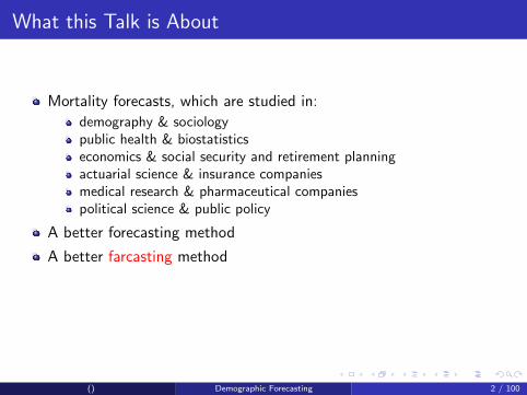
Mortality forecasts, which are studied in:
demography & sociologypublic health & biostatisticseconomics & social security and retirement planningactuarial science & insurance companiesmedical research & pharmaceutical companiespolitical science & public policy
A better forecasting method
A better farcasting method
Other results we needed to achieve this original goal
Approach: Formalizing qualitative insights in quantitative models
() Demographic Forecasting 2 / 100

What this Talk is About
Mortality forecasts, which are studied in:
demography & sociology
public health & biostatisticseconomics & social security and retirement planningactuarial science & insurance companiesmedical research & pharmaceutical companiespolitical science & public policy
A better forecasting method
A better farcasting method
Other results we needed to achieve this original goal
Approach: Formalizing qualitative insights in quantitative models
() Demographic Forecasting 2 / 100

What this Talk is About
Mortality forecasts, which are studied in:
demography & sociologypublic health & biostatistics
economics & social security and retirement planningactuarial science & insurance companiesmedical research & pharmaceutical companiespolitical science & public policy
A better forecasting method
A better farcasting method
Other results we needed to achieve this original goal
Approach: Formalizing qualitative insights in quantitative models
() Demographic Forecasting 2 / 100

What this Talk is About
Mortality forecasts, which are studied in:
demography & sociologypublic health & biostatisticseconomics & social security and retirement planning
actuarial science & insurance companiesmedical research & pharmaceutical companiespolitical science & public policy
A better forecasting method
A better farcasting method
Other results we needed to achieve this original goal
Approach: Formalizing qualitative insights in quantitative models
() Demographic Forecasting 2 / 100

What this Talk is About
Mortality forecasts, which are studied in:
demography & sociologypublic health & biostatisticseconomics & social security and retirement planningactuarial science & insurance companies
medical research & pharmaceutical companiespolitical science & public policy
A better forecasting method
A better farcasting method
Other results we needed to achieve this original goal
Approach: Formalizing qualitative insights in quantitative models
() Demographic Forecasting 2 / 100

What this Talk is About
Mortality forecasts, which are studied in:
demography & sociologypublic health & biostatisticseconomics & social security and retirement planningactuarial science & insurance companiesmedical research & pharmaceutical companies
political science & public policy
A better forecasting method
A better farcasting method
Other results we needed to achieve this original goal
Approach: Formalizing qualitative insights in quantitative models
() Demographic Forecasting 2 / 100

What this Talk is About
Mortality forecasts, which are studied in:
demography & sociologypublic health & biostatisticseconomics & social security and retirement planningactuarial science & insurance companiesmedical research & pharmaceutical companiespolitical science & public policy
A better forecasting method
A better farcasting method
Other results we needed to achieve this original goal
Approach: Formalizing qualitative insights in quantitative models
() Demographic Forecasting 2 / 100

What this Talk is About
Mortality forecasts, which are studied in:
demography & sociologypublic health & biostatisticseconomics & social security and retirement planningactuarial science & insurance companiesmedical research & pharmaceutical companiespolitical science & public policy
A better forecasting method
A better farcasting method
Other results we needed to achieve this original goal
Approach: Formalizing qualitative insights in quantitative models
() Demographic Forecasting 2 / 100

Other Results (Needed to Develop Improved Forecasts)
Output: same as linear regression
Estimates a set of linear regressions together (over countries, agegroups, years, etc.)
Can include different covariates in each regression
We demonstrate that most hierarchical and spatial Bayesian modelswith covariates misrepresent prior information
Better ways of creating Bayesian priors
Produces forecasts and farcasts using considerably more information
() Demographic Forecasting 3 / 100

Other Results (Needed to Develop Improved Forecasts)A New Class of Statistical Models
Output: same as linear regression
Estimates a set of linear regressions together (over countries, agegroups, years, etc.)
Can include different covariates in each regression
We demonstrate that most hierarchical and spatial Bayesian modelswith covariates misrepresent prior information
Better ways of creating Bayesian priors
Produces forecasts and farcasts using considerably more information
() Demographic Forecasting 3 / 100

The Statistical Problem of Global Mortality Forecasting
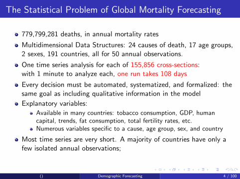
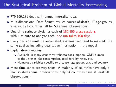
779,799,281 deaths, in annual mortality rates
Multidimensional Data Structures: 24 causes of death, 17 age groups,2 sexes, 191 countries, all for 50 annual observations.
One time series analysis for each of 155,856 cross-sections:
with 1 minute to analyze each, one run takes 108 days
Every decision must be automated, systematized, and formalized:
thesame goal as including qualitative information in the model
Explanatory variables:
Available in many countries: tobacco consumption, GDP, humancapital, trends, fat consumption, total fertility rates, etc.Numerous variables specific to a cause, age group, sex, and country
Most time series are very short.
A majority of countries have only afew isolated annual observations; only 54 countries have at least 20observations; Africa, AIDS, & Malaria are real problems
() Demographic Forecasting 4 / 100

The Statistical Problem of Global Mortality Forecasting
779,799,281 deaths, in annual mortality rates
Multidimensional Data Structures: 24 causes of death, 17 age groups,2 sexes, 191 countries, all for 50 annual observations.
One time series analysis for each of 155,856 cross-sections:with 1 minute to analyze each, one run takes 108 days
Every decision must be automated, systematized, and formalized: thesame goal as including qualitative information in the model
Explanatory variables:
Available in many countries: tobacco consumption, GDP, humancapital, trends, fat consumption, total fertility rates, etc.
Numerous variables specific to a cause, age group, sex, and country
Most time series are very short.
A majority of countries have only afew isolated annual observations; only 54 countries have at least 20observations; Africa, AIDS, & Malaria are real problems
() Demographic Forecasting 4 / 100

The Statistical Problem of Global Mortality Forecasting
779,799,281 deaths, in annual mortality rates
Multidimensional Data Structures: 24 causes of death, 17 age groups,2 sexes, 191 countries, all for 50 annual observations.
One time series analysis for each of 155,856 cross-sections:with 1 minute to analyze each, one run takes 108 days
Every decision must be automated, systematized, and formalized: thesame goal as including qualitative information in the model
Explanatory variables:
Available in many countries: tobacco consumption, GDP, humancapital, trends, fat consumption, total fertility rates, etc.Numerous variables specific to a cause, age group, sex, and country
Most time series are very short.
A majority of countries have only afew isolated annual observations; only 54 countries have at least 20observations; Africa, AIDS, & Malaria are real problems
() Demographic Forecasting 4 / 100

The Statistical Problem of Global Mortality Forecasting
779,799,281 deaths, in annual mortality rates
Multidimensional Data Structures: 24 causes of death, 17 age groups,2 sexes, 191 countries, all for 50 annual observations.
One time series analysis for each of 155,856 cross-sections:with 1 minute to analyze each, one run takes 108 days
Every decision must be automated, systematized, and formalized: thesame goal as including qualitative information in the model
Explanatory variables:
Available in many countries: tobacco consumption, GDP, humancapital, trends, fat consumption, total fertility rates, etc.Numerous variables specific to a cause, age group, sex, and country
Most time series are very short.
A majority of countries have only afew isolated annual observations; only 54 countries have at least 20observations; Africa, AIDS, & Malaria are real problems
() Demographic Forecasting 4 / 100
The Statistical Problem of Global Mortality Forecasting
779,799,281 deaths, in annual mortality rates
Multidimensional Data Structures: 24 causes of death, 17 age groups,2 sexes, 191 countries, all for 50 annual observations.
One time series analysis for each of 155,856 cross-sections:with 1 minute to analyze each, one run takes 108 days
Every decision must be automated, systematized, and formalized: thesame goal as including qualitative information in the model
Explanatory variables:
Available in many countries: tobacco consumption, GDP, humancapital, trends, fat consumption, total fertility rates, etc.Numerous variables specific to a cause, age group, sex, and country
Most time series are very short. A majority of countries have only afew isolated annual observations;
only 54 countries have at least 20observations; Africa, AIDS, & Malaria are real problems
() Demographic Forecasting 4 / 100
The Statistical Problem of Global Mortality Forecasting
779,799,281 deaths, in annual mortality rates
Multidimensional Data Structures: 24 causes of death, 17 age groups,2 sexes, 191 countries, all for 50 annual observations.
One time series analysis for each of 155,856 cross-sections:with 1 minute to analyze each, one run takes 108 days
Every decision must be automated, systematized, and formalized: thesame goal as including qualitative information in the model
Explanatory variables:
Available in many countries: tobacco consumption, GDP, humancapital, trends, fat consumption, total fertility rates, etc.Numerous variables specific to a cause, age group, sex, and country
Most time series are very short. A majority of countries have only afew isolated annual observations; only 54 countries have at least 20observations;
Africa, AIDS, & Malaria are real problems
() Demographic Forecasting 4 / 100

The Statistical Problem of Global Mortality Forecasting
779,799,281 deaths, in annual mortality rates
Multidimensional Data Structures: 24 causes of death, 17 age groups,2 sexes, 191 countries, all for 50 annual observations.
One time series analysis for each of 155,856 cross-sections:with 1 minute to analyze each, one run takes 108 days
Every decision must be automated, systematized, and formalized: thesame goal as including qualitative information in the model
Explanatory variables:
Available in many countries: tobacco consumption, GDP, humancapital, trends, fat consumption, total fertility rates, etc.Numerous variables specific to a cause, age group, sex, and country
Most time series are very short. A majority of countries have only afew isolated annual observations; only 54 countries have at least 20observations; Africa, AIDS, & Malaria are real problems
() Demographic Forecasting 4 / 100

Existing Method 1: Parameterize the Age Profile
−8
−6
−4
−2
0 5 10 15 20 25 30 35 40 45 50 55 60 65 70 75 80
All Causes (m)
Age
ln(m
orta
lity)
Japan
Turkey
Bolivia
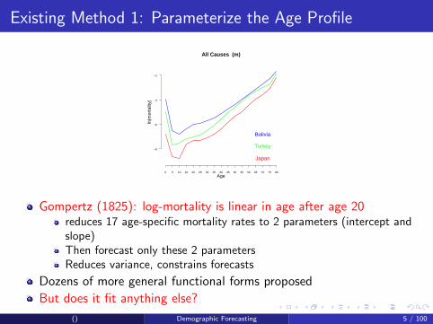
Gompertz (1825): log-mortality is linear in age after age 20
reduces 17 age-specific mortality rates to 2 parameters (intercept andslope)Then forecast only these 2 parametersReduces variance, constrains forecasts
Dozens of more general functional forms proposed
But does it fit anything else?
() Demographic Forecasting 5 / 100

Existing Method 1: Parameterize the Age Profile
−8
−6
−4
−2
0 5 10 15 20 25 30 35 40 45 50 55 60 65 70 75 80
All Causes (m)
Age
ln(m
orta
lity)
Japan
Turkey
Bolivia
Gompertz (1825): log-mortality is linear in age after age 20reduces 17 age-specific mortality rates to 2 parameters (intercept andslope)
Then forecast only these 2 parametersReduces variance, constrains forecasts
Dozens of more general functional forms proposed
But does it fit anything else?
() Demographic Forecasting 5 / 100

Existing Method 1: Parameterize the Age Profile
−8
−6
−4
−2
0 5 10 15 20 25 30 35 40 45 50 55 60 65 70 75 80
All Causes (m)
Age
ln(m
orta
lity)
Japan
Turkey
Bolivia
Gompertz (1825): log-mortality is linear in age after age 20reduces 17 age-specific mortality rates to 2 parameters (intercept andslope)Then forecast only these 2 parameters
Reduces variance, constrains forecasts
Dozens of more general functional forms proposed
But does it fit anything else?
() Demographic Forecasting 5 / 100

Existing Method 1: Parameterize the Age Profile
−8
−6
−4
−2
0 5 10 15 20 25 30 35 40 45 50 55 60 65 70 75 80
All Causes (m)
Age
ln(m
orta
lity)
Japan
Turkey
Bolivia
Gompertz (1825): log-mortality is linear in age after age 20reduces 17 age-specific mortality rates to 2 parameters (intercept andslope)Then forecast only these 2 parametersReduces variance, constrains forecasts
Dozens of more general functional forms proposed
But does it fit anything else?
() Demographic Forecasting 5 / 100

Mortality Age Profile: The Same Pattern?
−12
−10
−8
−6
−4
−2
0 5 10 15 20 25 30 35 40 45 50 55 60 65 70 75 80
Cardiovascular Disease (m)
Age
ln(m
orta
lity)
France
USA
Brazil
() Demographic Forecasting 6 / 100

Mortality Age Profile: The Same Pattern?
−16
−14
−12
−10
−8
−6
0 5 10 15 20 25 30 35 40 45 50 55 60 65 70 75 80
Breast Cancer (f)
Age
ln(m
orta
lity)
Japan
Venezuela
New Zealand
() Demographic Forecasting 7 / 100

Mortality Age Profile: The Same Pattern?
−12
−10
−8
−6
−4
0 5 10 15 20 25 30 35 40 45 50 55 60 65 70 75 80
Other Infectious Diseases (f)
Age
ln(m
orta
lity)
Italy
Barbados
Sri Lanka
Thailand
() Demographic Forecasting 8 / 100

Mortality Age Profile: The Same Pattern?
−10
−9
−8
−7
−6
15 20 25 30 35 40 45 50 55 60 65 70 75 80
Suicide (m)
Age
ln(m
orta
lity)
Sri Lanka
Colombia
Canada
Hungary
() Demographic Forecasting 9 / 100

Parameterizing Age Profiles Does Not Work
No mathematical form fits all or even most age profiles
Out-of-sample age profiles often unrealistic
The key empirical patterns are qualitative:
Adjacent age groups have similar mortality ratesAge profiles are more variable for younger agesWe don’t know much about levels or exact shapes
Key question: how to include this qualitative information
Also: Method ignores covariate information; the leading currentmethod (McNown-Rogers) not replicable
() Demographic Forecasting 10 / 100

Parameterizing Age Profiles Does Not Work
No mathematical form fits all or even most age profiles
Out-of-sample age profiles often unrealistic
The key empirical patterns are qualitative:
Adjacent age groups have similar mortality rates
Age profiles are more variable for younger agesWe don’t know much about levels or exact shapes
Key question: how to include this qualitative information
Also: Method ignores covariate information; the leading currentmethod (McNown-Rogers) not replicable
() Demographic Forecasting 10 / 100

Parameterizing Age Profiles Does Not Work
No mathematical form fits all or even most age profiles
Out-of-sample age profiles often unrealistic
The key empirical patterns are qualitative:
Adjacent age groups have similar mortality ratesAge profiles are more variable for younger ages
We don’t know much about levels or exact shapes
Key question: how to include this qualitative information
Also: Method ignores covariate information; the leading currentmethod (McNown-Rogers) not replicable
() Demographic Forecasting 10 / 100

Parameterizing Age Profiles Does Not Work
No mathematical form fits all or even most age profiles
Out-of-sample age profiles often unrealistic
The key empirical patterns are qualitative:
Adjacent age groups have similar mortality ratesAge profiles are more variable for younger agesWe don’t know much about levels or exact shapes
Key question: how to include this qualitative information
Also: Method ignores covariate information; the leading currentmethod (McNown-Rogers) not replicable
() Demographic Forecasting 10 / 100

Parameterizing Age Profiles Does Not Work
No mathematical form fits all or even most age profiles
Out-of-sample age profiles often unrealistic
The key empirical patterns are qualitative:
Adjacent age groups have similar mortality ratesAge profiles are more variable for younger agesWe don’t know much about levels or exact shapes
Key question: how to include this qualitative information
Also: Method ignores covariate information; the leading currentmethod (McNown-Rogers) not replicable
() Demographic Forecasting 10 / 100

Existing Method 2: Deterministic Projections
1960 1980 2000 2020 2040 2060
−10
−8−6
−4−2
All Causes (m) USA
Time
Dat
a an
d Fo
reca
sts
0
5
10
1520253035 404550
55
60
65
70
75
80
0 20 40 60 80
−10
−8−6
−4−2
All Causes (m) USA
Age
Dat
a an
d Fo
reca
sts
1950 2060
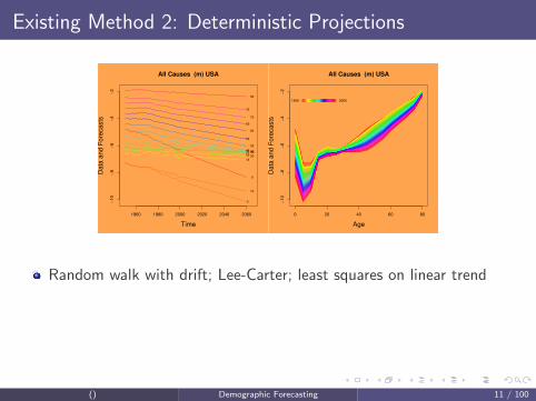
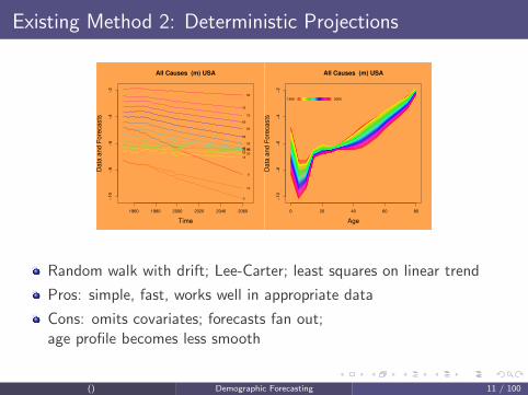
Random walk with drift; Lee-Carter; least squares on linear trend
Pros: simple, fast, works well in appropriate data
Cons: omits covariates
; forecasts fan out;age profile becomes less smooth
Does it fit elsewhere?
() Demographic Forecasting 11 / 100
Existing Method 2: Deterministic Projections
1960 1980 2000 2020 2040 2060
−10
−8−6
−4−2
All Causes (m) USA
Time
Dat
a an
d Fo
reca
sts
0
5
10
1520253035 404550
55
60
65
70
75
80
0 20 40 60 80
−10
−8−6
−4−2
All Causes (m) USA
Age
Dat
a an
d Fo
reca
sts
1950 2060
Random walk with drift; Lee-Carter; least squares on linear trend
Pros: simple, fast, works well in appropriate data
Cons: omits covariates
; forecasts fan out;age profile becomes less smooth
Does it fit elsewhere?
() Demographic Forecasting 11 / 100

Existing Method 2: Deterministic Projections
1960 1980 2000 2020 2040 2060
−10
−8−6
−4−2
All Causes (m) USA
Time
Dat
a an
d Fo
reca
sts
0
5
10
1520253035 404550
55
60
65
70
75
80
0 20 40 60 80
−10
−8−6
−4−2
All Causes (m) USA
Age
Dat
a an
d Fo
reca
sts
1950 2060
Random walk with drift; Lee-Carter; least squares on linear trend
Pros: simple, fast, works well in appropriate data
Cons: omits covariates; forecasts fan out
;age profile becomes less smooth
Does it fit elsewhere?
() Demographic Forecasting 11 / 100
Existing Method 2: Deterministic Projections
1960 1980 2000 2020 2040 2060
−10
−8−6
−4−2
All Causes (m) USA
Time
Dat
a an
d Fo
reca
sts
0
5
10
1520253035 404550
55
60
65
70
75
80
0 20 40 60 80
−10
−8−6
−4−2
All Causes (m) USA
Age
Dat
a an
d Fo
reca
sts
1950 2060
Random walk with drift; Lee-Carter; least squares on linear trend
Pros: simple, fast, works well in appropriate data
Cons: omits covariates; forecasts fan out;age profile becomes less smooth
Does it fit elsewhere?
() Demographic Forecasting 11 / 100

The same pattern?
1960 1980 2000 2020 2040 2060
−10.
5−1
0.0
−9.5
−9.0
−8.5
−8.0
−7.5
−7.0
Suicide (m) USA
Time
Dat
a an
d Fo
reca
sts
1520
25
30
35
40
45
50 5560
65
70
75
80
20 30 40 50 60 70 80
−10.
5−1
0.0
−9.5
−9.0
−8.5
−8.0
−7.5
−7.0
Suicide (m) USA
Age
Dat
a an
d Fo
reca
sts
1950 2060
() Demographic Forecasting 12 / 100

The same pattern?Random Walk with Drift ≈ Lee-Carter ≈ Least Squares
1960 1980 2000 2020 2040 2060
−10.
5−1
0.0
−9.5
−9.0
−8.5
−8.0
−7.5
−7.0
Suicide (m) USA
Time
Dat
a an
d Fo
reca
sts
1520
25
30
35
40
45
50 5560
65
70
75
80
20 30 40 50 60 70 80
−10.
5−1
0.0
−9.5
−9.0
−8.5
−8.0
−7.5
−7.0
Suicide (m) USA
Age
Dat
a an
d Fo
reca
sts
1950 2060
() Demographic Forecasting 12 / 100

The same pattern?
1960 1980 2000 2020 2040 2060
−10.
0−9
.5−9
.0−8
.5−8
.0−7
.5−7
.0−6
.5
Transportation Accidents (m) Portugal
Time
Dat
a an
d Fo
reca
sts
05
10
15
20
253035 40455055 60
65 70
7580
0 20 40 60 80
−10.
0−9
.5−9
.0−8
.5−8
.0−7
.5−7
.0−6
.5
Transportation Accidents (m) Portugal
Age
Dat
a an
d Fo
reca
sts
1955 2060
() Demographic Forecasting 13 / 100

The same pattern?Random Walk with Drift ≈ Lee-Carter ≈ Least Squares
1960 1980 2000 2020 2040 2060
−10.
0−9
.5−9
.0−8
.5−8
.0−7
.5−7
.0−6
.5
Transportation Accidents (m) Portugal
Time
Dat
a an
d Fo
reca
sts
05
10
15
20
253035 40455055 60
65 70
7580
0 20 40 60 80
−10.
0−9
.5−9
.0−8
.5−8
.0−7
.5−7
.0−6
.5
Transportation Accidents (m) Portugal
Age
Dat
a an
d Fo
reca
sts
1955 2060
() Demographic Forecasting 13 / 100

Deterministic Projections Do Not Work
Linearity does not fit most time series data
Out-of-sample age profiles become unrealistic over time
() Demographic Forecasting 14 / 100

Deterministic Projections Do Not Work
Linearity does not fit most time series data
Out-of-sample age profiles become unrealistic over time
() Demographic Forecasting 14 / 100

Deterministic Projections Do Not Work
Linearity does not fit most time series data
Out-of-sample age profiles become unrealistic over time
() Demographic Forecasting 14 / 100

Regression Approaches (Murray and Lopez, 1996)
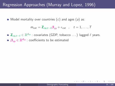
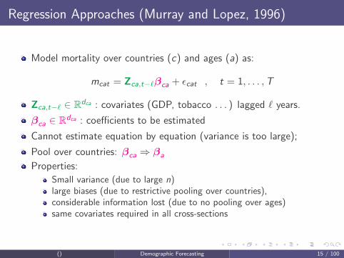
Model mortality over countries (c) and ages (a) as:
mcat = Zca,t−`βca + εcat , t = 1, . . . ,T
Zca,t−` ∈ Rdca : covariates (GDP, tobacco . . . ) lagged ` years.
βca ∈ Rdca : coefficients to be estimated
Cannot estimate equation by equation (variance is too large);
Pool over countries: βca ⇒ βa
Properties:
Small variance (due to large n)large biases (due to restrictive pooling over countries),considerable information lost (due to no pooling over ages)same covariates required in all cross-sections
() Demographic Forecasting 15 / 100

Regression Approaches (Murray and Lopez, 1996)
Model mortality over countries (c) and ages (a) as:
mcat = Zca,t−`βca + εcat , t = 1, . . . ,T
Zca,t−` ∈ Rdca : covariates (GDP, tobacco . . . ) lagged ` years.
βca ∈ Rdca : coefficients to be estimated
Cannot estimate equation by equation (variance is too large);
Pool over countries: βca ⇒ βa
Properties:
Small variance (due to large n)large biases (due to restrictive pooling over countries),considerable information lost (due to no pooling over ages)same covariates required in all cross-sections
() Demographic Forecasting 15 / 100

Regression Approaches (Murray and Lopez, 1996)
Model mortality over countries (c) and ages (a) as:
mcat = Zca,t−`βca + εcat , t = 1, . . . ,T
Zca,t−` ∈ Rdca : covariates (GDP, tobacco . . . ) lagged ` years.
βca ∈ Rdca : coefficients to be estimated
Cannot estimate equation by equation (variance is too large);
Pool over countries: βca ⇒ βa
Properties:
Small variance (due to large n)
large biases (due to restrictive pooling over countries),considerable information lost (due to no pooling over ages)same covariates required in all cross-sections
() Demographic Forecasting 15 / 100

Regression Approaches (Murray and Lopez, 1996)
Model mortality over countries (c) and ages (a) as:
mcat = Zca,t−`βca + εcat , t = 1, . . . ,T
Zca,t−` ∈ Rdca : covariates (GDP, tobacco . . . ) lagged ` years.
βca ∈ Rdca : coefficients to be estimated
Cannot estimate equation by equation (variance is too large);
Pool over countries: βca ⇒ βa
Properties:
Small variance (due to large n)large biases (due to restrictive pooling over countries),
considerable information lost (due to no pooling over ages)same covariates required in all cross-sections
() Demographic Forecasting 15 / 100

Regression Approaches (Murray and Lopez, 1996)
Model mortality over countries (c) and ages (a) as:
mcat = Zca,t−`βca + εcat , t = 1, . . . ,T
Zca,t−` ∈ Rdca : covariates (GDP, tobacco . . . ) lagged ` years.
βca ∈ Rdca : coefficients to be estimated
Cannot estimate equation by equation (variance is too large);
Pool over countries: βca ⇒ βa
Properties:
Small variance (due to large n)large biases (due to restrictive pooling over countries),considerable information lost (due to no pooling over ages)
same covariates required in all cross-sections
() Demographic Forecasting 15 / 100
Regression Approaches (Murray and Lopez, 1996)
Model mortality over countries (c) and ages (a) as:
mcat = Zca,t−`βca + εcat , t = 1, . . . ,T
Zca,t−` ∈ Rdca : covariates (GDP, tobacco . . . ) lagged ` years.
βca ∈ Rdca : coefficients to be estimated
Cannot estimate equation by equation (variance is too large);
Pool over countries: βca ⇒ βa
Properties:
Small variance (due to large n)large biases (due to restrictive pooling over countries),considerable information lost (due to no pooling over ages)same covariates required in all cross-sections
() Demographic Forecasting 15 / 100

Partial Pooling via a Bayesian Hierarchical Approach
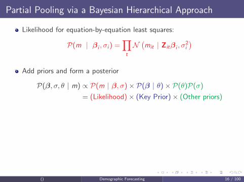
Likelihood for equation-by-equation least squares:
P(m | βi , σi ) =∏t
N(mit | Zitβi , σ
2i
)
Add priors and form a posterior
P(β, σ, θ | m) ∝ P(m | β, σ)× P(β | θ)× P(θ)P(σ)
= (Likelihood)× (Key Prior)× (Other priors)
Calculate point estimate for β (for y) as the mean posterior:
βBayes ≡∫
βP(β, σ, θ | m) dβdθdσ
The hard part: specifying the prior for β and, as always, Z
The easy part: easy-to-use software to implement everything wediscuss today.
() Demographic Forecasting 16 / 100
Partial Pooling via a Bayesian Hierarchical Approach
Likelihood for equation-by-equation least squares:
P(m | βi , σi ) =∏t
N(mit | Zitβi , σ
2i
)Add priors and form a posterior
P(β, σ, θ | m) ∝ P(m | β, σ)× P(β | θ)× P(θ)P(σ)
= (Likelihood)× (Key Prior)× (Other priors)
Calculate point estimate for β (for y) as the mean posterior:
βBayes ≡∫
βP(β, σ, θ | m) dβdθdσ
The hard part: specifying the prior for β and, as always, Z
The easy part: easy-to-use software to implement everything wediscuss today.
() Demographic Forecasting 16 / 100

The (Problematic) Classical Bayesian Approach
Assumption: similarities among cross-sections imply similarities amongcoefficients (β’s).
Requirements:
sij measures the similarity between cross-section i and j .(βi − βj)
′Φ(βi − βj) ≡ ‖βi − βj‖2Φ measures thedistance between βi and βj .
Natural choice for the prior:
P(β | Φ) ∝ exp
− 1
2
∑ij
sij‖βi − βj‖2Φ
() Demographic Forecasting 17 / 100

The (Problematic) Classical Bayesian Approach
Assumption: similarities among cross-sections imply similarities amongcoefficients (β’s).
Requirements:
sij measures the similarity between cross-section i and j .
(βi − βj)′Φ(βi − βj) ≡ ‖βi − βj‖2Φ measures the
distance between βi and βj .
Natural choice for the prior:
P(β | Φ) ∝ exp
− 1
2
∑ij
sij‖βi − βj‖2Φ
() Demographic Forecasting 17 / 100

The (Problematic) Classical Bayesian Approach
Assumption: similarities among cross-sections imply similarities amongcoefficients (β’s).
Requirements:
sij measures the similarity between cross-section i and j .(βi − βj)
′Φ(βi − βj) ≡ ‖βi − βj‖2Φ measures thedistance between βi and βj .
Natural choice for the prior:
P(β | Φ) ∝ exp
− 1
2
∑ij
sij‖βi − βj‖2Φ
() Demographic Forecasting 17 / 100

The (Problematic) Classical Bayesian Approach
Assumption: similarities among cross-sections imply similarities amongcoefficients (β’s).
Requirements:
sij measures the similarity between cross-section i and j .(βi − βj)
′Φ(βi − βj) ≡ ‖βi − βj‖2Φ measures thedistance between βi and βj .
Natural choice for the prior:
P(β | Φ) ∝ exp
− 1
2
∑ij
sij‖βi − βj‖2Φ
() Demographic Forecasting 17 / 100

The (Problematic) Classical Bayesian Approach
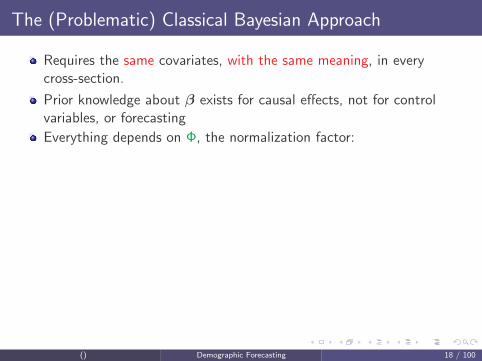
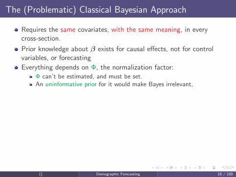
Requires the same covariates, with the same meaning, in everycross-section.
Prior knowledge about β exists for causal effects, not for controlvariables, or forecasting
Everything depends on Φ, the normalization factor:
Φ can’t be estimated, and must be set.An uninformative prior for it would make Bayes irrelevant,An informative prior can’t be used since we don’t have informationCommon practice: make some wild guesses.
The classical approach can be harmful: Making βi more smooth maymake µ less smooth (µ = Zβ):
µit − µjt = Zit(βi − βj) + (Zit − Zjt)βj
= Coefficient variation + Covariate variation
Extensive trial-and-error runs, yielded no useful parameter values.
() Demographic Forecasting 18 / 100

The (Problematic) Classical Bayesian Approach
Requires the same covariates, with the same meaning, in everycross-section.
Prior knowledge about β exists for causal effects, not for controlvariables, or forecasting
Everything depends on Φ, the normalization factor:
Φ can’t be estimated, and must be set.An uninformative prior for it would make Bayes irrelevant,An informative prior can’t be used since we don’t have informationCommon practice: make some wild guesses.
The classical approach can be harmful: Making βi more smooth maymake µ less smooth (µ = Zβ):
µit − µjt = Zit(βi − βj) + (Zit − Zjt)βj
= Coefficient variation + Covariate variation
Extensive trial-and-error runs, yielded no useful parameter values.
() Demographic Forecasting 18 / 100

The (Problematic) Classical Bayesian Approach
Requires the same covariates, with the same meaning, in everycross-section.
Prior knowledge about β exists for causal effects, not for controlvariables, or forecasting
Everything depends on Φ, the normalization factor:Φ can’t be estimated, and must be set.
An uninformative prior for it would make Bayes irrelevant,An informative prior can’t be used since we don’t have informationCommon practice: make some wild guesses.
The classical approach can be harmful: Making βi more smooth maymake µ less smooth (µ = Zβ):
µit − µjt = Zit(βi − βj) + (Zit − Zjt)βj
= Coefficient variation + Covariate variation
Extensive trial-and-error runs, yielded no useful parameter values.
() Demographic Forecasting 18 / 100
The (Problematic) Classical Bayesian Approach
Requires the same covariates, with the same meaning, in everycross-section.
Prior knowledge about β exists for causal effects, not for controlvariables, or forecasting
Everything depends on Φ, the normalization factor:Φ can’t be estimated, and must be set.An uninformative prior for it would make Bayes irrelevant,
An informative prior can’t be used since we don’t have informationCommon practice: make some wild guesses.
The classical approach can be harmful: Making βi more smooth maymake µ less smooth (µ = Zβ):
µit − µjt = Zit(βi − βj) + (Zit − Zjt)βj
= Coefficient variation + Covariate variation
Extensive trial-and-error runs, yielded no useful parameter values.
() Demographic Forecasting 18 / 100

The (Problematic) Classical Bayesian Approach
Requires the same covariates, with the same meaning, in everycross-section.
Prior knowledge about β exists for causal effects, not for controlvariables, or forecasting
Everything depends on Φ, the normalization factor:Φ can’t be estimated, and must be set.An uninformative prior for it would make Bayes irrelevant,An informative prior can’t be used since we don’t have information
Common practice: make some wild guesses.
The classical approach can be harmful: Making βi more smooth maymake µ less smooth (µ = Zβ):
µit − µjt = Zit(βi − βj) + (Zit − Zjt)βj
= Coefficient variation + Covariate variation
Extensive trial-and-error runs, yielded no useful parameter values.
() Demographic Forecasting 18 / 100
The (Problematic) Classical Bayesian Approach
Requires the same covariates, with the same meaning, in everycross-section.
Prior knowledge about β exists for causal effects, not for controlvariables, or forecasting
Everything depends on Φ, the normalization factor:Φ can’t be estimated, and must be set.An uninformative prior for it would make Bayes irrelevant,An informative prior can’t be used since we don’t have informationCommon practice: make some wild guesses.
The classical approach can be harmful: Making βi more smooth maymake µ less smooth (µ = Zβ):
µit − µjt = Zit(βi − βj) + (Zit − Zjt)βj
= Coefficient variation + Covariate variation
Extensive trial-and-error runs, yielded no useful parameter values.
() Demographic Forecasting 18 / 100

The (Problematic) Classical Bayesian Approach
Requires the same covariates, with the same meaning, in everycross-section.
Prior knowledge about β exists for causal effects, not for controlvariables, or forecasting
Everything depends on Φ, the normalization factor:Φ can’t be estimated, and must be set.An uninformative prior for it would make Bayes irrelevant,An informative prior can’t be used since we don’t have informationCommon practice: make some wild guesses.
The classical approach can be harmful: Making βi more smooth maymake µ less smooth (µ = Zβ):
µit − µjt
= Zit(βi − βj) + (Zit − Zjt)βj
= Coefficient variation + Covariate variation
Extensive trial-and-error runs, yielded no useful parameter values.
() Demographic Forecasting 18 / 100

The (Problematic) Classical Bayesian Approach
Requires the same covariates, with the same meaning, in everycross-section.
Prior knowledge about β exists for causal effects, not for controlvariables, or forecasting
Everything depends on Φ, the normalization factor:Φ can’t be estimated, and must be set.An uninformative prior for it would make Bayes irrelevant,An informative prior can’t be used since we don’t have informationCommon practice: make some wild guesses.
The classical approach can be harmful: Making βi more smooth maymake µ less smooth (µ = Zβ):
µit − µjt = Zit(βi − βj) + (Zit − Zjt)βj
= Coefficient variation + Covariate variation
Extensive trial-and-error runs, yielded no useful parameter values.
() Demographic Forecasting 18 / 100

The (Problematic) Classical Bayesian Approach
Requires the same covariates, with the same meaning, in everycross-section.
Prior knowledge about β exists for causal effects, not for controlvariables, or forecasting
Everything depends on Φ, the normalization factor:Φ can’t be estimated, and must be set.An uninformative prior for it would make Bayes irrelevant,An informative prior can’t be used since we don’t have informationCommon practice: make some wild guesses.
The classical approach can be harmful: Making βi more smooth maymake µ less smooth (µ = Zβ):
µit − µjt = Zit(βi − βj) + (Zit − Zjt)βj
= Coefficient variation + Covariate variation
Extensive trial-and-error runs, yielded no useful parameter values.
() Demographic Forecasting 18 / 100

Our Alternative Strategy: Priors on µ
Three steps:
1 Specify a prior for µ:
P(µ | θ) ∝ exp
(−1
2H[µ, θ]
), e.g., H[µ, θ] ≡ θ
T
T∑t=1
A−1∑a=1
(µat − µa+1,t)2
To do Bayes, we need a prior on βProblem: How to translate a prior on µ into a prior on β(a few-to-many transformation)?
2 Constrain the prior on µ to the subspace spanned by the covariates:µ = Zβ
3 In the subspace, we can invert µ = Zβ as β = (Z′Z)−1Z′µ, giving:
P(β | θ) ∝ exp
(−1
2H[µ, θ]
)= exp
(−1
2H[Zβ, θ]
)the same prior on µ, expressed as a function of β (with constantJacobian).
() Demographic Forecasting 19 / 100

Our Alternative Strategy: Priors on µ
Three steps:1 Specify a prior for µ:
P(µ | θ) ∝ exp
(−1
2H[µ, θ]
), e.g., H[µ, θ] ≡ θ
T
T∑t=1
A−1∑a=1
(µat − µa+1,t)2
To do Bayes, we need a prior on β
Problem: How to translate a prior on µ into a prior on β(a few-to-many transformation)?
2 Constrain the prior on µ to the subspace spanned by the covariates:µ = Zβ
3 In the subspace, we can invert µ = Zβ as β = (Z′Z)−1Z′µ, giving:
P(β | θ) ∝ exp
(−1
2H[µ, θ]
)= exp
(−1
2H[Zβ, θ]
)the same prior on µ, expressed as a function of β (with constantJacobian).
() Demographic Forecasting 19 / 100

Our Alternative Strategy: Priors on µ
Three steps:1 Specify a prior for µ:
P(µ | θ) ∝ exp
(−1
2H[µ, θ]
), e.g., H[µ, θ] ≡ θ
T
T∑t=1
A−1∑a=1
(µat − µa+1,t)2
To do Bayes, we need a prior on βProblem: How to translate a prior on µ into a prior on β(a few-to-many transformation)?
2 Constrain the prior on µ to the subspace spanned by the covariates:µ = Zβ
3 In the subspace, we can invert µ = Zβ as β = (Z′Z)−1Z′µ, giving:
P(β | θ) ∝ exp
(−1
2H[µ, θ]
)= exp
(−1
2H[Zβ, θ]
)the same prior on µ, expressed as a function of β (with constantJacobian).
() Demographic Forecasting 19 / 100

Our Alternative Strategy: Priors on µ
Three steps:1 Specify a prior for µ:
P(µ | θ) ∝ exp
(−1
2H[µ, θ]
), e.g., H[µ, θ] ≡ θ
T
T∑t=1
A−1∑a=1
(µat − µa+1,t)2
To do Bayes, we need a prior on βProblem: How to translate a prior on µ into a prior on β(a few-to-many transformation)?
2 Constrain the prior on µ to the subspace spanned by the covariates:µ = Zβ
3 In the subspace, we can invert µ = Zβ as β = (Z′Z)−1Z′µ, giving:
P(β | θ) ∝ exp
(−1
2H[µ, θ]
)= exp
(−1
2H[Zβ, θ]
)the same prior on µ, expressed as a function of β (with constantJacobian).
() Demographic Forecasting 19 / 100

Say that again?
In other words
Any prior information about µ (the expected value of the dependentvariable) is “translated” into information about the coefficients β via
µcat = Zcatβca
A Simple Analogy
Suppose δ = β1 − β2 and P(δ) = N(δ|0, σ2)
What is P(β1, β2)?
Its a singular bivariate Normal
Its defined over β1, β2 and constant in all directions but (β1 − β2).
We start with one-dimensional P(µcat), and treat it as themultidimensional P(βca), constant in all directions but Zcatβca.
() Demographic Forecasting 20 / 100

Advantages of the resulting prior over β, created fromprior over µ
Fully Bayesian: The same theory of inference applies
Can use standard Bayesian machinery for estimation.
µi and µj can always be compared, even with different covariates.
The normalization matrix Φ is unnecessary (task is performed by Z,which is known)
Priors are based on knowledge rather than guesses.
() Demographic Forecasting 21 / 100

An Age Prior
P(µ | θ) P(β | θ) ∝ exp
(−θ∑aa′
W naa′β′
aCaa′βa′
)
The prior is normal (and improper);
Adjustable parameters: n and θ.
The choice of n uniquely determines the “interaction” matrix W n
The variance of the prior is inversely proportional to θ, which controlsthe “strength” of the prior.
Different age groups can have different covariates: the matricesCaa′ ≡ 1
T Z′aZa′ are rectangular (da × da′).
() Demographic Forecasting 22 / 100

Samples From Age Prior
0 20 40 60 80
−8−6
−4−2
All Causes (m) , n = 1
Age
Log−
mor
talit
y
() Demographic Forecasting 23 / 100

Samples From Age Prior
0 20 40 60 80
−8−6
−4−2
All Causes (m) , n = 2
Age
Log−
mor
talit
y
() Demographic Forecasting 24 / 100

Samples From Age Prior
0 20 40 60 80
−8−6
−4−2
All Causes (m) , n = 3
Age
Log−
mor
talit
y
() Demographic Forecasting 25 / 100

Samples From Age Prior
0 20 40 60 80
−8−6
−4−2
All Causes (m) , n = 4
Age
Log−
mor
talit
y
() Demographic Forecasting 26 / 100

Samples From Age Prior
0 20 40 60 80
−8−6
−4−2
All Causes (m) , n = 1
Age
Log−
mor
talit
y
0 20 40 60 80
−8−6
−4−2
All Causes (m) , n = 2
Age
Log−
mor
talit
y
0 20 40 60 80
−8−6
−4−2
All Causes (m) , n = 3
Age
Log−
mor
talit
y
0 20 40 60 80
−8−6
−4−2
All Causes (m) , n = 4
Age
Log−
mor
talit
y
() Demographic Forecasting 27 / 100

Prior Indifference
These priors are “indifferent” to transformations:
µ(a, t) µ(a, t) + p(a, t)
where p(a, t) is a polynomial in a (whose degree is the degree of thederivative in the prior)
Prior information is about relative (not absolute) levels oflog-mortality
() Demographic Forecasting 28 / 100

Prior Indifference
These priors are “indifferent” to transformations:
µ(a, t) µ(a, t) + p(a, t)
where p(a, t) is a polynomial in a (whose degree is the degree of thederivative in the prior)
Prior information is about relative (not absolute) levels oflog-mortality
() Demographic Forecasting 28 / 100

Prior Indifference
These priors are “indifferent” to transformations:
µ(a, t) µ(a, t) + p(a, t)
where p(a, t) is a polynomial in a (whose degree is the degree of thederivative in the prior)
Prior information is about relative (not absolute) levels oflog-mortality
() Demographic Forecasting 28 / 100

Prior Indifference
These priors are “indifferent” to transformations:
µ(a, t) µ(a, t) + p(a, t)
where p(a, t) is a polynomial in a (whose degree is the degree of thederivative in the prior)
Prior information is about relative (not absolute) levels oflog-mortality
() Demographic Forecasting 28 / 100

Formalizing (Prior) Indifferenceequal color = equal probability
Level indifference
0 20 40 60 80
−10
−8
−6
−4
−2
0
All Causes (m) , n = 1
Age
Log−
mor
talit
y
Level and slope indifference
0 20 40 60 80
−8
−6
−4
−2
02
All Causes (m) , n = 2
Age
Log−
mor
talit
y
() Demographic Forecasting 29 / 100
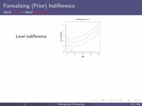
Formalizing (Prior) Indifferenceequal color = equal probability
Level indifference
0 20 40 60 80
−10
−8
−6
−4
−2
0
All Causes (m) , n = 1
Age
Log−
mor
talit
y
Level and slope indifference
0 20 40 60 80
−8
−6
−4
−2
02
All Causes (m) , n = 2
Age
Log−
mor
talit
y
() Demographic Forecasting 29 / 100

Formalizing (Prior) Indifferenceequal color = equal probability
Level indifference
0 20 40 60 80
−10
−8
−6
−4
−2
0
All Causes (m) , n = 1
Age
Log−
mor
talit
y
Level and slope indifference
0 20 40 60 80
−8
−6
−4
−2
02
All Causes (m) , n = 2
Age
Log−
mor
talit
y
() Demographic Forecasting 29 / 100

Smoothness Parameter
The prior:
P(β | θ) ∝ exp
(−θ∑aa′
W naa′β′
aCaa′βa′
)
We figured out what n is
but what is the smoothness parameter, θ?
θ controls the prior standard deviation
() Demographic Forecasting 30 / 100

Smoothness Parameter
The prior:
P(β | θ) ∝ exp
(−θ∑aa′
W naa′β′
aCaa′βa′
)
We figured out what n is
but what is the smoothness parameter, θ?
θ controls the prior standard deviation
() Demographic Forecasting 30 / 100
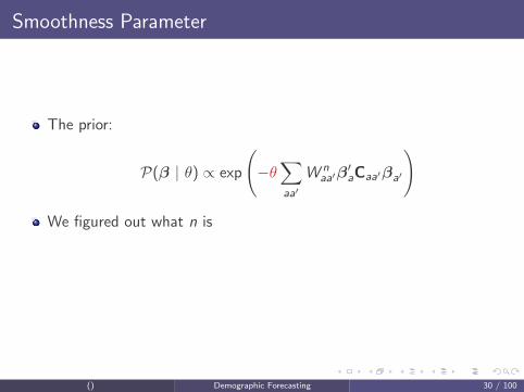
Smoothness Parameter
The prior:
P(β | θ) ∝ exp
(−θ∑aa′
W naa′β′
aCaa′βa′
)
We figured out what n is
but what is the smoothness parameter, θ?
θ controls the prior standard deviation
() Demographic Forecasting 30 / 100

Smoothness Parameter
The prior:
P(β | θ) ∝ exp
(−θ∑aa′
W naa′β′
aCaa′βa′
)
We figured out what n is
but what is the smoothness parameter, θ?
θ controls the prior standard deviation
() Demographic Forecasting 30 / 100
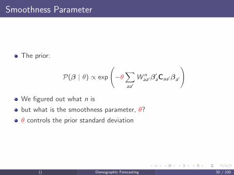
Smoothness Parameter
The prior:
P(β | θ) ∝ exp
(−θ∑aa′
W naa′β′
aCaa′βa′
)
We figured out what n is
but what is the smoothness parameter, θ?
θ controls the prior standard deviation
() Demographic Forecasting 30 / 100

Samples from Age Prior
0 20 40 60 80
−10
−8−6
−4−2
02
All Causes (f) , n = 2
Age
Log−
mor
talit
y
() Demographic Forecasting 31 / 100

Samples from Age Prior
0 20 40 60 80
−10
−8−6
−4−2
02
All Causes (f) , n = 2
Age
Log−
mor
talit
y
() Demographic Forecasting 32 / 100

Samples from Age Prior
0 20 40 60 80
−10
−8−6
−4−2
02
All Causes (f) , n = 2
Age
Log−
mor
talit
y
() Demographic Forecasting 33 / 100

Samples from Age Prior
0 20 40 60 80
−10
−8−6
−4−2
02
All Causes (f) , n = 2
Age
Log−
mor
talit
y
() Demographic Forecasting 34 / 100

Samples from Age Prior
0 20 40 60 80
−10
−8−6
−4−2
02
All Causes (f) , n = 2
Age
Log−
mor
talit
y
() Demographic Forecasting 35 / 100

Samples from Age Prior
0 20 40 60 80
−10
−8−6
−4−2
02
All Causes (f) , n = 2
Age
Log−
mor
talit
y
() Demographic Forecasting 36 / 100

Samples from Age Prior
0 20 40 60 80
−10
−8−6
−4−2
02
All Causes (f) , n = 2
Age
Log−
mor
talit
y
() Demographic Forecasting 37 / 100

Samples from Age Prior
0 20 40 60 80
−10
−8−6
−4−2
02
All Causes (f) , n = 2
Age
Log−
mor
talit
y
() Demographic Forecasting 38 / 100
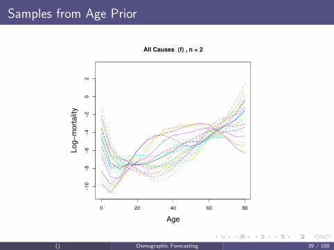
Samples from Age Prior
0 20 40 60 80
−10
−8−6
−4−2
02
All Causes (f) , n = 2
Age
Log−
mor
talit
y
() Demographic Forecasting 39 / 100
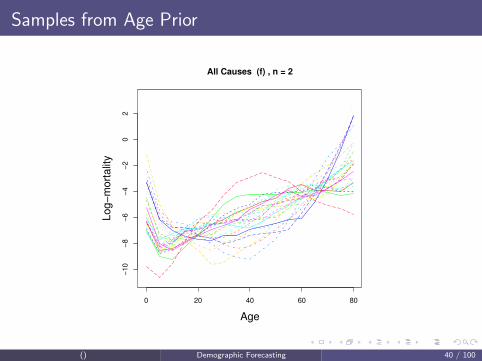
Samples from Age Prior
0 20 40 60 80
−10
−8−6
−4−2
02
All Causes (f) , n = 2
Age
Log−
mor
talit
y
() Demographic Forecasting 40 / 100

Samples from Age Prior
0 20 40 60 80
−10
−8−6
−4−2
02
All Causes (f) , n = 2
Age
Log−
mor
talit
y
() Demographic Forecasting 41 / 100

Samples from Age Prior
0 20 40 60 80
−10
−8−6
−4−2
02
All Causes (f) , n = 2
Age
Log−
mor
talit
y
() Demographic Forecasting 42 / 100

Samples from Age Prior
0 20 40 60 80
−10
−8−6
−4−2
02
All Causes (f) , n = 2
Age
Log−
mor
talit
y
() Demographic Forecasting 43 / 100

Generalizations
The above tools: smooth over a (possibly discretized) continuousvariable — age or age groups.
We can also smooth over time (also a discretized continuous variable).
Can smooth when cross-sectional unit i is a label, such as country.
Can smooth simultaneously over different types of variables (age,country, and time).
We can smooth interactions:
Smoothing trends over age groups.Smoothing trends over age groups as they vary across countries, etc.
The mathematical form for all these (separately or together) turns outto be the same:
P(β | θ) ∝ exp
−θ
2
∑ij
Wijβ′iCijβj
, Caa′ ≡ 1
TZaZa′
() Demographic Forecasting 44 / 100
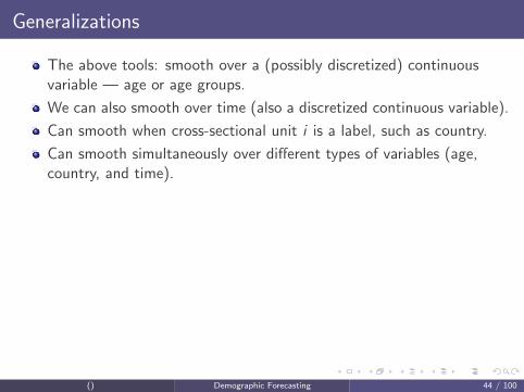
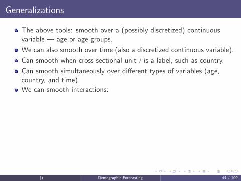

Generalizations
The above tools: smooth over a (possibly discretized) continuousvariable — age or age groups.
We can also smooth over time (also a discretized continuous variable).
Can smooth when cross-sectional unit i is a label, such as country.
Can smooth simultaneously over different types of variables (age,country, and time).
We can smooth interactions:Smoothing trends over age groups.
Smoothing trends over age groups as they vary across countries, etc.
The mathematical form for all these (separately or together) turns outto be the same:
P(β | θ) ∝ exp
−θ
2
∑ij
Wijβ′iCijβj
, Caa′ ≡ 1
TZaZa′
() Demographic Forecasting 44 / 100

Generalizations
The above tools: smooth over a (possibly discretized) continuousvariable — age or age groups.
We can also smooth over time (also a discretized continuous variable).
Can smooth when cross-sectional unit i is a label, such as country.
Can smooth simultaneously over different types of variables (age,country, and time).
We can smooth interactions:Smoothing trends over age groups.Smoothing trends over age groups as they vary across countries, etc.
The mathematical form for all these (separately or together) turns outto be the same:
P(β | θ) ∝ exp
−θ
2
∑ij
Wijβ′iCijβj
, Caa′ ≡ 1
TZaZa′
() Demographic Forecasting 44 / 100

Mortality from Respiratory Infections, MalesLeast Squares
0 20 40 60 80
−10
−8−6
−4
(m) Belize
Age
Dat
a an
d Fo
reca
sts
1970 2030
() Demographic Forecasting 45 / 100

Mortality from Respiratory Infections, males, σ = 2.00Smoothing over Age Groups
0 20 40 60 80
−12
−10
−8−6
−4
(m) Belize
Age
Dat
a an
d F
orec
asts
1970 2030
() Demographic Forecasting 46 / 100

Mortality from Respiratory Infections, males, σ = 1.51Smoothing over Age Groups
0 20 40 60 80
−12
−10
−8−6
−4
(m) Belize
Age
Dat
a an
d F
orec
asts
1970 2030
() Demographic Forecasting 47 / 100

Mortality from Respiratory Infections, males, σ = 1.15Smoothing over Age Groups
0 20 40 60 80
−12
−10
−8−6
−4
(m) Belize
Age
Dat
a an
d F
orec
asts
1970 2030
() Demographic Forecasting 48 / 100
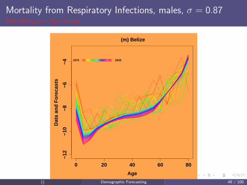
Mortality from Respiratory Infections, males, σ = 0.87Smoothing over Age Groups
0 20 40 60 80
−12
−10
−8−6
−4
(m) Belize
Age
Dat
a an
d F
orec
asts
1970 2030
() Demographic Forecasting 49 / 100

Mortality from Respiratory Infections, males, σ = 0.66Smoothing over Age Groups
0 20 40 60 80
−12
−10
−8−6
−4
(m) Belize
Age
Dat
a an
d F
orec
asts
1970 2030
() Demographic Forecasting 50 / 100

Mortality from Respiratory Infections, males, σ = 0.50Smoothing over Age Groups
0 20 40 60 80
−12
−10
−8−6
−4
(m) Belize
Age
Dat
a an
d F
orec
asts
1970 2030
() Demographic Forecasting 51 / 100

Mortality from Respiratory Infections, males, σ = 0.38Smoothing over Age Groups
0 20 40 60 80
−12
−10
−8−6
−4
(m) Belize
Age
Dat
a an
d F
orec
asts
1970 2030
() Demographic Forecasting 52 / 100

Mortality from Respiratory Infections, males, σ = 0.28Smoothing over Age Groups
0 20 40 60 80
−12
−10
−8−6
−4
(m) Belize
Age
Dat
a an
d F
orec
asts
1970 2030
() Demographic Forecasting 53 / 100

Mortality from Respiratory Infections, males, σ = 0.21Smoothing over Age Groups
0 20 40 60 80
−12
−10
−8−6
−4
(m) Belize
Age
Dat
a an
d F
orec
asts
1970 2030
() Demographic Forecasting 54 / 100

Mortality from Respiratory Infections, males, σ = 0.16Smoothing over Age Groups
0 20 40 60 80
−12
−10
−8−6
−4
(m) Belize
Age
Dat
a an
d F
orec
asts
1970 2030
() Demographic Forecasting 55 / 100

Mortality from Respiratory Infections, males, σ = 0.12Smoothing over Age Groups
0 20 40 60 80
−12
−10
−8−6
−4
(m) Belize
Age
Dat
a an
d F
orec
asts
1970 2030
() Demographic Forecasting 56 / 100

Mortality from Respiratory Infections, males, σ = 0.09Smoothing over Age Groups
0 20 40 60 80
−12
−10
−8−6
−4
(m) Belize
Age
Dat
a an
d F
orec
asts
1970 2030
() Demographic Forecasting 57 / 100

Mortality from Respiratory Infections, males, σ = 0.07Smoothing over Age Groups
0 20 40 60 80
−12
−10
−8−6
−4
(m) Belize
Age
Dat
a an
d F
orec
asts
1970 2030
() Demographic Forecasting 58 / 100

Mortality from Respiratory Infections, males, σ = 0.05Smoothing over Age Groups
0 20 40 60 80
−12
−10
−8−6
−4
(m) Belize
Age
Dat
a an
d F
orec
asts
1970 2030
() Demographic Forecasting 59 / 100
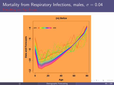
Mortality from Respiratory Infections, males, σ = 0.04Smoothing over Age Groups
0 20 40 60 80
−12
−10
−8−6
−4
(m) Belize
Age
Dat
a an
d F
orec
asts
1970 2030
() Demographic Forecasting 60 / 100

Mortality from Respiratory Infections, males, σ = 0.03Smoothing over Age Groups
0 20 40 60 80
−12
−10
−8−6
−4
(m) Belize
Age
Dat
a an
d F
orec
asts
1970 2030
() Demographic Forecasting 61 / 100

Mortality from Respiratory Infections, males, σ = 0.02Smoothing over Age Groups
0 20 40 60 80
−12
−10
−8−6
−4
(m) Belize
Age
Dat
a an
d F
orec
asts
1970 2030
() Demographic Forecasting 62 / 100

Mortality from Respiratory Infections, males, σ = 0.01Smoothing over Age Groups
0 20 40 60 80
−12
−10
−8−6
−4
(m) Belize
Age
Dat
a an
d F
orec
asts
1970 2030
() Demographic Forecasting 63 / 100

Mortality from Respiratory Infections, malesLeast Squares
1970 1980 1990 2000 2010 2020 2030
−12
−10
−8−6
−4
(m) Belize
Time
Dat
a an
d F
orec
asts
0
5
10
15
20
25
30 35
4045
50
55
60
65
70
75
80
() Demographic Forecasting 64 / 100

Mortality from Respiratory Infections, males, σ = 2.00Smoothing over Age Groups
1970 1980 1990 2000 2010 2020 2030
−12
−10
−8−6
−4
(m) Belize
Time
Dat
a an
d F
orec
asts
0
5
10
15
2025
30 3540 4550 55
60
65
70
75
80
() Demographic Forecasting 65 / 100

Mortality from Respiratory Infections, males, σ = 1.51Smoothing over Age Groups
1970 1980 1990 2000 2010 2020 2030
−12
−10
−8−6
−4
(m) Belize
Time
Dat
a an
d F
orec
asts
0
5
10
15
2025
30 3540 4550
55
60
65
70
75
80
() Demographic Forecasting 66 / 100

Mortality from Respiratory Infections, males, σ = 1.15Smoothing over Age Groups
1970 1980 1990 2000 2010 2020 2030
−12
−10
−8−6
−4
(m) Belize
Time
Dat
a an
d F
orec
asts
0
5
10
15
2025
30 3540 4550
55
60
65
70
75
80
() Demographic Forecasting 67 / 100
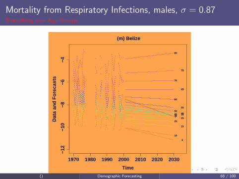
Mortality from Respiratory Infections, males, σ = 0.87Smoothing over Age Groups
1970 1980 1990 2000 2010 2020 2030
−12
−10
−8−6
−4
(m) Belize
Time
Dat
a an
d F
orec
asts
0
5
10
15
2025
30 3540 4550
55
60
65
70
75
80
() Demographic Forecasting 68 / 100

Mortality from Respiratory Infections, males, σ = 0.66Smoothing over Age Groups
1970 1980 1990 2000 2010 2020 2030
−12
−10
−8−6
−4
(m) Belize
Time
Dat
a an
d F
orec
asts
0
5
10
15
2025
30354045
50
55
60
65
70
75
80
() Demographic Forecasting 69 / 100

Mortality from Respiratory Infections, males, σ = 0.50Smoothing over Age Groups
1970 1980 1990 2000 2010 2020 2030
−12
−10
−8−6
−4
(m) Belize
Time
Dat
a an
d F
orec
asts
0
510
15
2025
3035
4045
50
55
60
65
70
75
80
() Demographic Forecasting 70 / 100

Mortality from Respiratory Infections, males, σ = 0.38Smoothing over Age Groups
1970 1980 1990 2000 2010 2020 2030
−12
−10
−8−6
−4
(m) Belize
Time
Dat
a an
d F
orec
asts
0
510
15
2025
3035
4045
50
55
60
65
70
75
80
() Demographic Forecasting 71 / 100
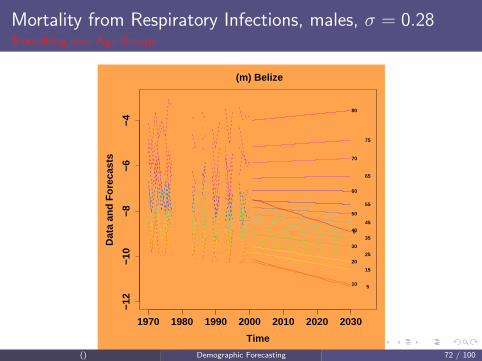
Mortality from Respiratory Infections, males, σ = 0.28Smoothing over Age Groups
1970 1980 1990 2000 2010 2020 2030
−12
−10
−8−6
−4
(m) Belize
Time
Dat
a an
d F
orec
asts
0
510
15
2025
30
35
40
45
50
55
60
65
70
75
80
() Demographic Forecasting 72 / 100

Mortality from Respiratory Infections, males, σ = 0.21Smoothing over Age Groups
1970 1980 1990 2000 2010 2020 2030
−12
−10
−8−6
−4
(m) Belize
Time
Dat
a an
d F
orec
asts
0
510
15
20
25
30
35
40
45
50
55
60
65
70
75
80
() Demographic Forecasting 73 / 100

Mortality from Respiratory Infections, males, σ = 0.16Smoothing over Age Groups
1970 1980 1990 2000 2010 2020 2030
−12
−10
−8−6
−4
(m) Belize
Time
Dat
a an
d F
orec
asts
0
510
1520
25
30
35
40
45
50
55
60
65
70
75
80
() Demographic Forecasting 74 / 100
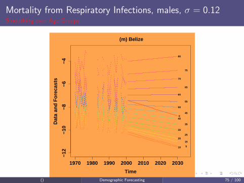
Mortality from Respiratory Infections, males, σ = 0.12Smoothing over Age Groups
1970 1980 1990 2000 2010 2020 2030
−12
−10
−8−6
−4
(m) Belize
Time
Dat
a an
d F
orec
asts
0
510
1520
25
30
35
40
45
50
55
60
65
70
75
80
() Demographic Forecasting 75 / 100

Mortality from Respiratory Infections, males, σ = 0.09Smoothing over Age Groups
1970 1980 1990 2000 2010 2020 2030
−12
−10
−8−6
−4
(m) Belize
Time
Dat
a an
d F
orec
asts
0
510
1520
25
30
35
40
45
50
55
60
65
70
75
80
() Demographic Forecasting 76 / 100

Mortality from Respiratory Infections, males, σ = 0.07Smoothing over Age Groups
1970 1980 1990 2000 2010 2020 2030
−12
−10
−8−6
−4
(m) Belize
Time
Dat
a an
d F
orec
asts
0
510
1520
25
30
35
40
45
50
55
60
65
70
75
80
() Demographic Forecasting 77 / 100

Mortality from Respiratory Infections, males, σ = 0.05Smoothing over Age Groups
1970 1980 1990 2000 2010 2020 2030
−12
−10
−8−6
−4
(m) Belize
Time
Dat
a an
d F
orec
asts
0
510
1520
25
30
35
40
45
50
55
60
65
70
75
80
() Demographic Forecasting 78 / 100

Mortality from Respiratory Infections, males, σ = 0.04Smoothing over Age Groups
1970 1980 1990 2000 2010 2020 2030
−12
−10
−8−6
−4
(m) Belize
Time
Dat
a an
d F
orec
asts
0
510
1520
25
30
35
40
45
50
55
60
65
70
75
80
() Demographic Forecasting 79 / 100

Mortality from Respiratory Infections, males, σ = 0.03Smoothing over Age Groups
1970 1980 1990 2000 2010 2020 2030
−12
−10
−8−6
−4
(m) Belize
Time
Dat
a an
d F
orec
asts
0
510
1520
25
30
35
40
45
50
55
60
65
70
75
80
() Demographic Forecasting 80 / 100

Mortality from Respiratory Infections, males, σ = 0.02Smoothing over Age Groups
1970 1980 1990 2000 2010 2020 2030
−12
−10
−8−6
−4
(m) Belize
Time
Dat
a an
d F
orec
asts
0
510
1520
25
30
35
40
45
50
55
60
65
70
75
80
() Demographic Forecasting 81 / 100

Mortality from Respiratory Infections, males, σ = 0.01Smoothing over Age Groups
1970 1980 1990 2000 2010 2020 2030
−12
−10
−8−6
−4
(m) Belize
Time
Dat
a an
d F
orec
asts
0
510
1520
25
30
35
40
45
50
55
60
65
70
75
80
() Demographic Forecasting 82 / 100

Smoothing Trends over Age Groups
Least Squares
1970 1980 1990 2000 2010 2020 2030
−10
−9−8
−7−6
−5−4
(m) Belize
Time
Dat
a an
d Fo
reca
sts
0
5
10
1520
25
30
35
40
45
50
55
60
65
70
75
80
0 20 40 60 80
−10
−8−6
−4
(m) Belize
Age
Dat
a an
d Fo
reca
sts
1970 2030
SmoothingAge Groups
1970 1980 1990 2000 2010 2020 2030
−10
−8−6
−4
(m) Belize
Time
Dat
a an
d Fo
reca
sts
0
510
15
20
25
30
35
40
45
50
55
60
65
70
75
80
0 20 40 60 80
−10
−8−6
−4
(m) Belize
Age
Dat
a an
d Fo
reca
sts
1970 2030
() Demographic Forecasting 83 / 100

Smoothing Trends over Age GroupsLog-mortality in Belize males from respiratory infections
Least Squares
1970 1980 1990 2000 2010 2020 2030
−10
−9−8
−7−6
−5−4
(m) Belize
Time
Dat
a an
d Fo
reca
sts
0
5
10
1520
25
30
35
40
45
50
55
60
65
70
75
80
0 20 40 60 80
−10
−8−6
−4
(m) Belize
Age
Dat
a an
d Fo
reca
sts
1970 2030
SmoothingAge Groups
1970 1980 1990 2000 2010 2020 2030
−10
−8−6
−4
(m) Belize
Time
Dat
a an
d Fo
reca
sts
0
510
15
20
25
30
35
40
45
50
55
60
65
70
75
80
0 20 40 60 80
−10
−8−6
−4
(m) Belize
Age
Dat
a an
d Fo
reca
sts
1970 2030
() Demographic Forecasting 83 / 100
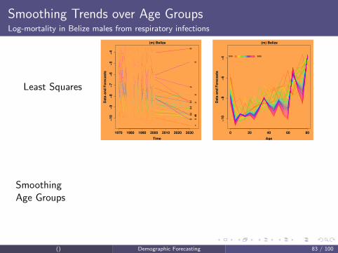
Smoothing Trends over Age GroupsLog-mortality in Belize males from respiratory infections
Least Squares
1970 1980 1990 2000 2010 2020 2030
−10
−9−8
−7−6
−5−4
(m) Belize
Time
Dat
a an
d Fo
reca
sts
0
5
10
1520
25
30
35
40
45
50
55
60
65
70
75
80
0 20 40 60 80
−10
−8−6
−4
(m) Belize
Age
Dat
a an
d Fo
reca
sts
1970 2030
SmoothingAge Groups
1970 1980 1990 2000 2010 2020 2030
−10
−8−6
−4
(m) Belize
Time
Dat
a an
d Fo
reca
sts
0
510
15
20
25
30
35
40
45
50
55
60
65
70
75
80
0 20 40 60 80
−10
−8−6
−4
(m) Belize
Age
Dat
a an
d Fo
reca
sts
1970 2030
() Demographic Forecasting 83 / 100

Smoothing Trends over Age Groups and Time
Least Squares
1970 1990 2010 2030
−11
−10
−9−8
−7−6
−5−4
(m) Bulgaria
Time
Dat
a an
d Fo
reca
sts
0
5
10
1520
25
30
35
4045
50 5560
65
70
75
80
0 20 40 60 80
−12
−10
−8−6
−4
(m) Bulgaria
Age
Dat
a an
d Fo
reca
sts
1964 2030
SmoothingAge and Time
1970 1990 2010 2030
−11
−10
−9−8
−7−6
−5−4
(m) Bulgaria
Time
Dat
a an
d Fo
reca
sts
0
5
10
1520
25
30
35
40
4550
5560
65
70
75
80
0 20 40 60 80
−12
−10
−8−6
−4
(m) Bulgaria
Age
Dat
a an
d Fo
reca
sts
1964 2030
() Demographic Forecasting 84 / 100
Smoothing Trends over Age Groups and TimeLog-Mortality in Bulgarian males from respiratory infections
Least Squares
1970 1990 2010 2030
−11
−10
−9−8
−7−6
−5−4
(m) Bulgaria
Time
Dat
a an
d Fo
reca
sts
0
5
10
1520
25
30
35
4045
50 5560
65
70
75
80
0 20 40 60 80
−12
−10
−8−6
−4
(m) Bulgaria
Age
Dat
a an
d Fo
reca
sts
1964 2030
SmoothingAge and Time
1970 1990 2010 2030
−11
−10
−9−8
−7−6
−5−4
(m) Bulgaria
Time
Dat
a an
d Fo
reca
sts
0
5
10
1520
25
30
35
40
4550
5560
65
70
75
80
0 20 40 60 80
−12
−10
−8−6
−4
(m) Bulgaria
Age
Dat
a an
d Fo
reca
sts
1964 2030
() Demographic Forecasting 84 / 100
Using Covariates (GDP, tobacco, trend, log trend)
Least Squares
1990 2000 2010 2020 2030
−10
−50
5
(m) Republic of Korea
Time
Dat
a an
d F
orec
asts
30
3540
45
50
5560 65
70
7580
30 40 50 60 70 80
−10
−50
5
(m) Republic of Korea
Age
Dat
a an
d F
orec
asts
1985 2030
Smooth over age,time, age/time
1990 2000 2010 2020 2030
−14
−12
−10
−8−6
−4
(m) Republic of Korea
Time
Dat
a an
d F
orec
asts
30
35
40
45
50
55
60
65
70
75
80
30 40 50 60 70 80
−14
−12
−10
−8−6
−4
(m) Republic of Korea
Age
Dat
a an
d F
orec
asts
1985 2030
() Demographic Forecasting 85 / 100

Using Covariates (GDP, tobacco, trend, log trend)Lung cancer in Korean Males
Least Squares
1990 2000 2010 2020 2030
−10
−50
5
(m) Republic of Korea
Time
Dat
a an
d F
orec
asts
30
3540
45
50
5560 65
70
7580
30 40 50 60 70 80
−10
−50
5
(m) Republic of Korea
Age
Dat
a an
d F
orec
asts
1985 2030
Smooth over age,time, age/time
1990 2000 2010 2020 2030
−14
−12
−10
−8−6
−4
(m) Republic of Korea
Time
Dat
a an
d F
orec
asts
30
35
40
45
50
55
60
65
70
75
80
30 40 50 60 70 80
−14
−12
−10
−8−6
−4
(m) Republic of Korea
Age
Dat
a an
d F
orec
asts
1985 2030
() Demographic Forecasting 85 / 100

Using Covariates (GDP, tobacco, trend, log trend)
Least Squares
1970 1990 2010 2030
−20
−15
−10
−50
(m) Singapore
Time
Dat
a an
d F
orec
asts
30
35
40
4550
55
60
65
707580
30 40 50 60 70 80
−20
−15
−10
−50
(m) Singapore
Age
Dat
a an
d F
orec
asts
1963 2030
Smooth over age,time, age/time
1970 1990 2010 2030
−14
−12
−10
−8−6
(m) Singapore
Time
Dat
a an
d F
orec
asts
30
35
40
45
50
55
60
65
70
7580
30 40 50 60 70 80
−14
−12
−10
−8−6
(m) Singapore
Age
Dat
a an
d F
orec
asts
1963 2030
() Demographic Forecasting 86 / 100

Using Covariates (GDP, tobacco, trend, log trend)Lung cancer in Males, Singapore
Least Squares
1970 1990 2010 2030
−20
−15
−10
−50
(m) Singapore
Time
Dat
a an
d F
orec
asts
30
35
40
4550
55
60
65
707580
30 40 50 60 70 80
−20
−15
−10
−50
(m) Singapore
Age
Dat
a an
d F
orec
asts
1963 2030
Smooth over age,time, age/time
1970 1990 2010 2030
−14
−12
−10
−8−6
(m) Singapore
Time
Dat
a an
d F
orec
asts
30
35
40
45
50
55
60
65
70
7580
30 40 50 60 70 80
−14
−12
−10
−8−6
(m) Singapore
Age
Dat
a an
d F
orec
asts
1963 2030
() Demographic Forecasting 86 / 100
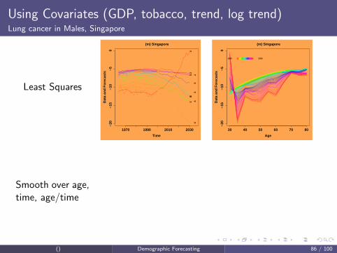
Using Covariates (GDP, tobacco, trend, log trend)Lung cancer in Males, Singapore
Least Squares
1970 1990 2010 2030
−20
−15
−10
−50
(m) Singapore
Time
Dat
a an
d F
orec
asts
30
35
40
4550
55
60
65
707580
30 40 50 60 70 80
−20
−15
−10
−50
(m) Singapore
Age
Dat
a an
d F
orec
asts
1963 2030
Smooth over age,time, age/time
1970 1990 2010 2030
−14
−12
−10
−8−6
(m) Singapore
Time
Dat
a an
d F
orec
asts
30
35
40
45
50
55
60
65
70
7580
30 40 50 60 70 80
−14
−12
−10
−8−6
(m) Singapore
Age
Dat
a an
d F
orec
asts
1963 2030
() Demographic Forecasting 86 / 100
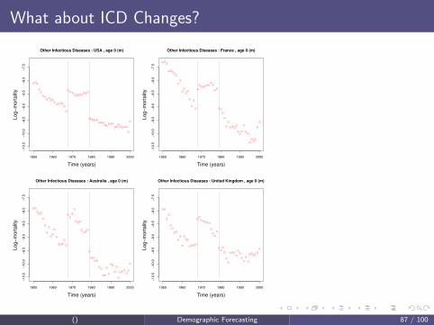
What about ICD Changes?
1950 1960 1970 1980 1990 2000
−10.
5−1
0.0
−9.5
−9.0
−8.5
−8.0
−7.5
Other Infectious Diseases : USA , age 0 (m)
Time (years)
Log−
mor
talit
y
1950 1960 1970 1980 1990 2000−1
0.5
−10.
0−9
.5−9
.0−8
.5−8
.0−7
.5
Other Infectious Diseases : France , age 0 (m)
Time (years)
Log−
mor
talit
y
1950 1960 1970 1980 1990 2000
−10.
5−1
0.0
−9.5
−9.0
−8.5
−8.0
−7.5
Other Infectious Diseases : Australia , age 0 (m)
Time (years)
Log−
mor
talit
y
1950 1960 1970 1980 1990 2000
−10.
5−1
0.0
−9.5
−9.0
−8.5
−8.0
−7.5
Other Infectious Diseases : United Kingdom , age 0 (m)
Time (years)
Log−
mor
talit
y
() Demographic Forecasting 87 / 100

Fixing ICD Changes
1950 1960 1970 1980 1990 2000
−10.
5−1
0.0
−9.5
−9.0
−8.5
−8.0
−7.5
Other Infectious Diseases : USA , age 0 (m)
Time (years)
Log−
mor
talit
y
1950 1960 1970 1980 1990 2000−1
0.5
−10.
0−9
.5−9
.0−8
.5−8
.0−7
.5
Other Infectious Diseases : France , age 0 (m)
Time (years)
Log−
mor
talit
y
1950 1960 1970 1980 1990 2000
−10.
5−1
0.0
−9.5
−9.0
−8.5
−8.0
−7.5
Other Infectious Diseases : Australia , age 0 (m)
Time (years)
Log−
mor
talit
y
1950 1960 1970 1980 1990 2000
−10.
5−1
0.0
−9.5
−9.0
−8.5
−8.0
−7.5
Other Infectious Diseases : United Kingdom , age 0 (m)
Time (years)
Log−
mor
talit
y
() Demographic Forecasting 88 / 100

A book manuscript, YourCast software, etc.
http://GKing.Harvard.edu
() Demographic Forecasting 89 / 100

Preview of Results: Out-of-Sample Evaluation
% Improvement
Over Best to BestPrevious Conceivable
Cardiovascular 22 49Lung Cancer 24 47
Transportation 16 31Respiratory Chronic 13 30
Other Infectious 12 30Stomach Cancer 8 24
All-Cause 12 22Suicide 7 17
Respiratory Infectious 3 7
Each row averages 6,800 forecast errors (17 age groups, 40 countries, and10 out-of-sample years).% to best conceivable = % of the way our method takes us from the bestexisting to the best conceivable forecast.The new method out-performs with the same covariates, for mostcountries, causes, sexes, and age groups.Does considerably better with more informative covariates
() Demographic Forecasting 90 / 100
Preview of Results: Out-of-Sample EvaluationMean Absolute Error in Males (over age and country)
% Improvement
Over Best to BestPrevious Conceivable
Cardiovascular 22 49Lung Cancer 24 47
Transportation 16 31Respiratory Chronic 13 30
Other Infectious 12 30Stomach Cancer 8 24
All-Cause 12 22Suicide 7 17
Respiratory Infectious 3 7
Each row averages 6,800 forecast errors (17 age groups, 40 countries, and10 out-of-sample years).% to best conceivable = % of the way our method takes us from the bestexisting to the best conceivable forecast.The new method out-performs with the same covariates, for mostcountries, causes, sexes, and age groups.Does considerably better with more informative covariates
() Demographic Forecasting 90 / 100

Preview of Results: Out-of-Sample EvaluationMean Absolute Error in Males (over age and country)
% Improvement
Over Best to BestPrevious Conceivable
Cardiovascular 22 49Lung Cancer 24 47
Transportation 16 31Respiratory Chronic 13 30
Other Infectious 12 30Stomach Cancer 8 24
All-Cause 12 22Suicide 7 17
Respiratory Infectious 3 7
Each row averages 6,800 forecast errors (17 age groups, 40 countries, and10 out-of-sample years).
% to best conceivable = % of the way our method takes us from the bestexisting to the best conceivable forecast.The new method out-performs with the same covariates, for mostcountries, causes, sexes, and age groups.Does considerably better with more informative covariates
() Demographic Forecasting 90 / 100

Preview of Results: Out-of-Sample EvaluationMean Absolute Error in Males (over age and country)
% Improvement
Over Best to BestPrevious Conceivable
Cardiovascular 22 49Lung Cancer 24 47
Transportation 16 31Respiratory Chronic 13 30
Other Infectious 12 30Stomach Cancer 8 24
All-Cause 12 22Suicide 7 17
Respiratory Infectious 3 7
Each row averages 6,800 forecast errors (17 age groups, 40 countries, and10 out-of-sample years).% to best conceivable = % of the way our method takes us from the bestexisting to the best conceivable forecast.
The new method out-performs with the same covariates, for mostcountries, causes, sexes, and age groups.Does considerably better with more informative covariates
() Demographic Forecasting 90 / 100

Preview of Results: Out-of-Sample EvaluationMean Absolute Error in Males (over age and country)
% Improvement
Over Best to BestPrevious Conceivable
Cardiovascular 22 49Lung Cancer 24 47
Transportation 16 31Respiratory Chronic 13 30
Other Infectious 12 30Stomach Cancer 8 24
All-Cause 12 22Suicide 7 17
Respiratory Infectious 3 7
Each row averages 6,800 forecast errors (17 age groups, 40 countries, and10 out-of-sample years).% to best conceivable = % of the way our method takes us from the bestexisting to the best conceivable forecast.The new method out-performs with the same covariates, for mostcountries, causes, sexes, and age groups.
Does considerably better with more informative covariates
() Demographic Forecasting 90 / 100

Preview of Results: Out-of-Sample EvaluationMean Absolute Error in Males (over age and country)
% Improvement
Over Best to BestPrevious Conceivable
Cardiovascular 22 49Lung Cancer 24 47
Transportation 16 31Respiratory Chronic 13 30
Other Infectious 12 30Stomach Cancer 8 24
All-Cause 12 22Suicide 7 17
Respiratory Infectious 3 7
Each row averages 6,800 forecast errors (17 age groups, 40 countries, and10 out-of-sample years).% to best conceivable = % of the way our method takes us from the bestexisting to the best conceivable forecast.The new method out-performs with the same covariates, for mostcountries, causes, sexes, and age groups.Does considerably better with more informative covariates
() Demographic Forecasting 90 / 100

Basic Prior: Smoothness over Age Groups
Prior knowledge: log-mortality age profile are smooth variations of a“typical” age profile µ(a):
H[µ, θ] ≡
θ
AT
∫ T
0dt
∫ A
0da
(dn
dan[µ(a, t)− µ(a)]
)2
Discretize age and time:
P(µ | θ) ∝ exp
(− 1
2θ∑aa′t
(µat − µa)′W n
aa′(µa′t − µa′)
)
where W n is a matrix uniquely determined by n and θ
() Demographic Forecasting 91 / 100
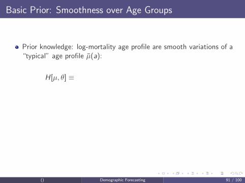

Basic Prior: Smoothness over Age Groups
Prior knowledge: log-mortality age profile are smooth variations of a“typical” age profile µ(a):
H[µ, θ] ≡
θ
AT
∫ T
0dt
∫ A
0da
(dn
dan
[µ(a, t)− µ(a)]
)2
Discretize age and time:
P(µ | θ) ∝ exp
(− 1
2θ∑aa′t
(µat − µa)′W n
aa′(µa′t − µa′)
)
where W n is a matrix uniquely determined by n and θ
() Demographic Forecasting 91 / 100

Basic Prior: Smoothness over Age Groups
Prior knowledge: log-mortality age profile are smooth variations of a“typical” age profile µ(a):
H[µ, θ] ≡
θ
AT
∫ T
0dt
∫ A
0da
(
dn
dan[µ(a, t)− µ(a)]
)2
Discretize age and time:
P(µ | θ) ∝ exp
(− 1
2θ∑aa′t
(µat − µa)′W n
aa′(µa′t − µa′)
)
where W n is a matrix uniquely determined by n and θ
() Demographic Forecasting 91 / 100

Basic Prior: Smoothness over Age Groups
Prior knowledge: log-mortality age profile are smooth variations of a“typical” age profile µ(a):
H[µ, θ] ≡
θ
AT
∫ T
0dt
∫ A
0da
(dn
dan[µ(a, t)− µ(a)]
)2
Discretize age and time:
P(µ | θ) ∝ exp
(− 1
2θ∑aa′t
(µat − µa)′W n
aa′(µa′t − µa′)
)
where W n is a matrix uniquely determined by n and θ
() Demographic Forecasting 91 / 100

Basic Prior: Smoothness over Age Groups
Prior knowledge: log-mortality age profile are smooth variations of a“typical” age profile µ(a):
H[µ, θ] ≡ θ
AT
∫ T
0dt
∫ A
0da
(dn
dan[µ(a, t)− µ(a)]
)2
Discretize age and time:
P(µ | θ) ∝ exp
(− 1
2θ∑aa′t
(µat − µa)′W n
aa′(µa′t − µa′)
)
where W n is a matrix uniquely determined by n and θ
() Demographic Forecasting 91 / 100

From a prior on µ to a prior on β
Add the specification µat = µa + Zatβa:
P(β | θ) = exp
(− θ
T
∑aa′t
W naa′(Zatβa)(Za′tβa′)
)
= exp
(−θ∑aa′
W naa′β′
aCaa′βa′
)
where we have defined:
Caa′ ≡ 1
TZ′
aZa′ Za is a T × da data matrix for age group a
() Demographic Forecasting 92 / 100

From a prior on µ to a prior on β
Add the specification µat = µa + Zatβa:
P(β | θ) = exp
(− θ
T
∑aa′t
W naa′(Zatβa)(Za′tβa′)
)
= exp
(−θ∑aa′
W naa′β′
aCaa′βa′
)
where we have defined:
Caa′ ≡ 1
TZ′
aZa′ Za is a T × da data matrix for age group a
() Demographic Forecasting 92 / 100

From a prior on µ to a prior on β
Add the specification µat = µa + Zatβa:
P(β | θ) = exp
(− θ
T
∑aa′t
W naa′(Zatβa)(Za′tβa′)
)
= exp
(−θ∑aa′
W naa′β′
aCaa′βa′
)
where we have defined:
Caa′ ≡ 1
TZ′
aZa′ Za is a T × da data matrix for age group a
() Demographic Forecasting 92 / 100

From a prior on µ to a prior on β
Add the specification µat = µa + Zatβa:
P(β | θ) = exp
(− θ
T
∑aa′t
W naa′(Zatβa)(Za′tβa′)
)
= exp
(−θ∑aa′
W naa′β′
aCaa′βa′
)
where we have defined:
Caa′ ≡ 1
TZ′
aZa′ Za is a T × da data matrix for age group a
() Demographic Forecasting 92 / 100

The Prior on the Coefficients β
P(β | θ) ∝ exp
(−θ∑aa′
W naa′β′
aCaa′βa′
)
The prior is normal (and improper);
The prior is uniquely determined by the choice of n, through the“interaction” matrix W n.
Different age groups can have different covariates: the matrices Caa′
are rectangular (da × da′).
The variance of the prior is inversely proportional to θ, which controlsthe “strength” of the prior.
() Demographic Forecasting 93 / 100

Without Country Smoothing
−12
−10
−8
−6
−4
1950 1970 1990 2010 2030
Age 0
1950 1970 1990 2010 2030
Age 5
1950 1970 1990 2010 2030
Age 10
1950 1970 1990 2010 2030
Age 15
−12
−10
−8
−6
−4
1950 1970 1990 2010 2030
Age 20
1950 1970 1990 2010 2030
Age 25
1950 1970 1990 2010 2030
Age 30
1950 1970 1990 2010 2030
Age 35
−12
−10
−8
−6
−4
1950 1970 1990 2010 2030
Age 40
1950 1970 1990 2010 2030
Age 45
1950 1970 1990 2010 2030
Age 50
1950 1970 1990 2010 2030
Age 55
−12
−10
−8
−6
−4
1950 1970 1990 2010 2030
Age 60
1950 1970 1990 2010 2030
Age 65
1950 1970 1990 2010 2030
Age 70
1950 1970 1990 2010 2030
Age 75
−12
−10
−8
−6
−4
1950 1970 1990 2010 2030
Age 80
0 20 40 60 80
Out of Sample
0 20 40 60 80
In Sample
TransportationAccidents
(males)Sri Lanka
CXC
() Demographic Forecasting 94 / 100

With Country Smoothing
−12
−10
−8
−6
−4
1950 1970 1990 2010 2030
Age 0
1950 1970 1990 2010 2030
Age 5
1950 1970 1990 2010 2030
Age 10
1950 1970 1990 2010 2030
Age 15
−12
−10
−8
−6
−4
1950 1970 1990 2010 2030
Age 20
1950 1970 1990 2010 2030
Age 25
1950 1970 1990 2010 2030
Age 30
1950 1970 1990 2010 2030
Age 35
−12
−10
−8
−6
−4
1950 1970 1990 2010 2030
Age 40
1950 1970 1990 2010 2030
Age 45
1950 1970 1990 2010 2030
Age 50
1950 1970 1990 2010 2030
Age 55
−12
−10
−8
−6
−4
1950 1970 1990 2010 2030
Age 60
1950 1970 1990 2010 2030
Age 65
1950 1970 1990 2010 2030
Age 70
1950 1970 1990 2010 2030
Age 75
−12
−10
−8
−6
−4
1950 1970 1990 2010 2030
Age 80
0 20 40 60 80
Out of Sample
0 20 40 60 80
In Sample
TransportationAccidents
(males)Sri Lanka
BAYES
() Demographic Forecasting 95 / 100

Formalizing Similarity
Standard Bayesian Approach
Assume coefficients are similar
— But we know little about the coefficients
Requires the same covariates in each cross-section
— Why measure water quality in the U.S.?
Requires covariates with the same meaning in each cross-section
— Does GDP mean the same thing in Botswana and the U.S.?
Imposes no assumptions on covariates or mortality
— If covariates are dissimilar, then making coefficients similar makesmortality dissimilar [since E (yt) = Xtβ in each cross-section]
Alternative Approach
Assume expected mortality is similarCoefficients are unobserved, mortality patterns are well knownDifferent covariates allowed in each cross-sectionCovariates with the same name can have different meanings
() Demographic Forecasting 96 / 100
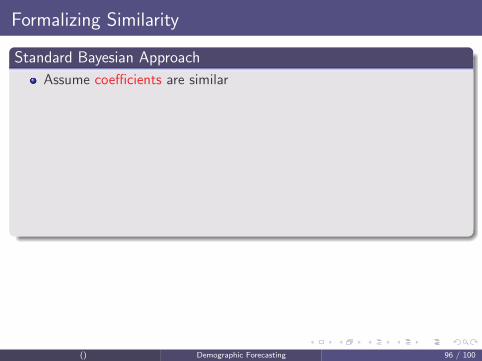
Formalizing Similarity
Standard Bayesian Approach
Assume coefficients are similar
— But we know little about the coefficientsRequires the same covariates in each cross-section
— Why measure water quality in the U.S.?
Requires covariates with the same meaning in each cross-section
— Does GDP mean the same thing in Botswana and the U.S.?
Imposes no assumptions on covariates or mortality
— If covariates are dissimilar, then making coefficients similar makesmortality dissimilar [since E (yt) = Xtβ in each cross-section]
Alternative Approach
Assume expected mortality is similarCoefficients are unobserved, mortality patterns are well knownDifferent covariates allowed in each cross-sectionCovariates with the same name can have different meanings
() Demographic Forecasting 96 / 100

Formalizing Similarity
Standard Bayesian Approach
Assume coefficients are similar— But we know little about the coefficients
Requires the same covariates in each cross-section
— Why measure water quality in the U.S.?
Requires covariates with the same meaning in each cross-section
— Does GDP mean the same thing in Botswana and the U.S.?
Imposes no assumptions on covariates or mortality
— If covariates are dissimilar, then making coefficients similar makesmortality dissimilar [since E (yt) = Xtβ in each cross-section]
Alternative Approach
Assume expected mortality is similarCoefficients are unobserved, mortality patterns are well knownDifferent covariates allowed in each cross-sectionCovariates with the same name can have different meanings
() Demographic Forecasting 96 / 100

Formalizing Similarity
Standard Bayesian Approach
Assume coefficients are similar— But we know little about the coefficientsRequires the same covariates in each cross-section
— Why measure water quality in the U.S.?Requires covariates with the same meaning in each cross-section
— Does GDP mean the same thing in Botswana and the U.S.?
Imposes no assumptions on covariates or mortality
— If covariates are dissimilar, then making coefficients similar makesmortality dissimilar [since E (yt) = Xtβ in each cross-section]
Alternative Approach
Assume expected mortality is similarCoefficients are unobserved, mortality patterns are well knownDifferent covariates allowed in each cross-sectionCovariates with the same name can have different meanings
() Demographic Forecasting 96 / 100

Formalizing Similarity
Standard Bayesian Approach
Assume coefficients are similar— But we know little about the coefficientsRequires the same covariates in each cross-section— Why measure water quality in the U.S.?
Requires covariates with the same meaning in each cross-section
— Does GDP mean the same thing in Botswana and the U.S.?
Imposes no assumptions on covariates or mortality
— If covariates are dissimilar, then making coefficients similar makesmortality dissimilar [since E (yt) = Xtβ in each cross-section]
Alternative Approach
Assume expected mortality is similarCoefficients are unobserved, mortality patterns are well knownDifferent covariates allowed in each cross-sectionCovariates with the same name can have different meanings
() Demographic Forecasting 96 / 100

Formalizing Similarity
Standard Bayesian Approach
Assume coefficients are similar— But we know little about the coefficientsRequires the same covariates in each cross-section— Why measure water quality in the U.S.?Requires covariates with the same meaning in each cross-section
— Does GDP mean the same thing in Botswana and the U.S.?Imposes no assumptions on covariates or mortality
— If covariates are dissimilar, then making coefficients similar makesmortality dissimilar [since E (yt) = Xtβ in each cross-section]
Alternative Approach
Assume expected mortality is similarCoefficients are unobserved, mortality patterns are well knownDifferent covariates allowed in each cross-sectionCovariates with the same name can have different meanings
() Demographic Forecasting 96 / 100

Formalizing Similarity
Standard Bayesian Approach
Assume coefficients are similar— But we know little about the coefficientsRequires the same covariates in each cross-section— Why measure water quality in the U.S.?Requires covariates with the same meaning in each cross-section— Does GDP mean the same thing in Botswana and the U.S.?
Imposes no assumptions on covariates or mortality
— If covariates are dissimilar, then making coefficients similar makesmortality dissimilar [since E (yt) = Xtβ in each cross-section]
Alternative Approach
Assume expected mortality is similarCoefficients are unobserved, mortality patterns are well knownDifferent covariates allowed in each cross-sectionCovariates with the same name can have different meanings
() Demographic Forecasting 96 / 100

Formalizing Similarity
Standard Bayesian Approach
Assume coefficients are similar— But we know little about the coefficientsRequires the same covariates in each cross-section— Why measure water quality in the U.S.?Requires covariates with the same meaning in each cross-section— Does GDP mean the same thing in Botswana and the U.S.?Imposes no assumptions on covariates or mortality
— If covariates are dissimilar, then making coefficients similar makesmortality dissimilar [since E (yt) = Xtβ in each cross-section]
Alternative Approach
Assume expected mortality is similarCoefficients are unobserved, mortality patterns are well knownDifferent covariates allowed in each cross-sectionCovariates with the same name can have different meanings
() Demographic Forecasting 96 / 100

Formalizing Similarity
Standard Bayesian Approach
Assume coefficients are similar— But we know little about the coefficientsRequires the same covariates in each cross-section— Why measure water quality in the U.S.?Requires covariates with the same meaning in each cross-section— Does GDP mean the same thing in Botswana and the U.S.?Imposes no assumptions on covariates or mortality— If covariates are dissimilar, then making coefficients similar makesmortality dissimilar [since E (yt) = Xtβ in each cross-section]
Alternative Approach
Assume expected mortality is similar
Coefficients are unobserved, mortality patterns are well knownDifferent covariates allowed in each cross-sectionCovariates with the same name can have different meanings
() Demographic Forecasting 96 / 100

Formalizing Similarity
Standard Bayesian Approach
Assume coefficients are similar— But we know little about the coefficientsRequires the same covariates in each cross-section— Why measure water quality in the U.S.?Requires covariates with the same meaning in each cross-section— Does GDP mean the same thing in Botswana and the U.S.?Imposes no assumptions on covariates or mortality— If covariates are dissimilar, then making coefficients similar makesmortality dissimilar [since E (yt) = Xtβ in each cross-section]
Alternative Approach
Assume expected mortality is similarCoefficients are unobserved, mortality patterns are well known
Different covariates allowed in each cross-sectionCovariates with the same name can have different meanings
() Demographic Forecasting 96 / 100
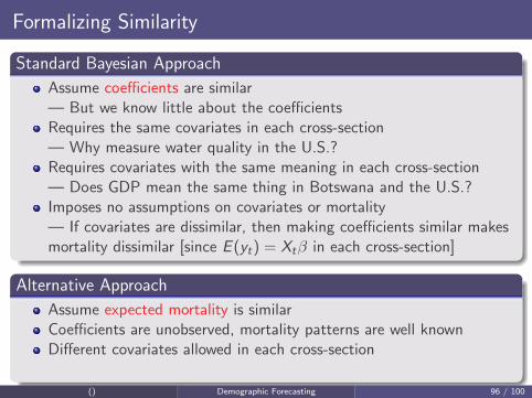
Formalizing Similarity
Standard Bayesian Approach
Assume coefficients are similar— But we know little about the coefficientsRequires the same covariates in each cross-section— Why measure water quality in the U.S.?Requires covariates with the same meaning in each cross-section— Does GDP mean the same thing in Botswana and the U.S.?Imposes no assumptions on covariates or mortality— If covariates are dissimilar, then making coefficients similar makesmortality dissimilar [since E (yt) = Xtβ in each cross-section]
Alternative Approach
Assume expected mortality is similarCoefficients are unobserved, mortality patterns are well knownDifferent covariates allowed in each cross-section
Covariates with the same name can have different meanings
() Demographic Forecasting 96 / 100

Formalizing Similarity
Standard Bayesian Approach
Assume coefficients are similar— But we know little about the coefficientsRequires the same covariates in each cross-section— Why measure water quality in the U.S.?Requires covariates with the same meaning in each cross-section— Does GDP mean the same thing in Botswana and the U.S.?Imposes no assumptions on covariates or mortality— If covariates are dissimilar, then making coefficients similar makesmortality dissimilar [since E (yt) = Xtβ in each cross-section]
Alternative Approach
Assume expected mortality is similarCoefficients are unobserved, mortality patterns are well knownDifferent covariates allowed in each cross-sectionCovariates with the same name can have different meanings
() Demographic Forecasting 96 / 100

Many Short Time Series
10 20 30 40 50
0.2
0.4
0.6
0.8
1.0
Coverage of WHO data base (age specific, all causes)
# Observations
%
●
●●
●
●●●
●●●●●
●●
●●
●●●
●
●
●●●●
●
●●
●●●●
●
●●●●
●●●●●●●●●
●●●●●
●●●
●●●●●
●●
●●●●
●
% of world countries
% of world population
() Demographic Forecasting 97 / 100

Preview of Results: Out-of-Sample Evaluation
Mean Absolute Error % Improvement
Best Our Best Over Best to BestPrevious Method Conceivable Previous Conceivable
Cardiovascular 0.34 0.27 0.19 22 49Lung Cancer 0.36 0.27 0.17 24 47
Transportation 0.37 0.31 0.18 16 31Respiratory Chronic 0.45 0.39 0.26 13 30
Other Infectious 0.55 0.48 0.32 12 30Stomach Cancer 0.30 0.27 0.20 8 24
All-Cause 0.17 0.15 0.08 12 22Suicide 0.31 0.29 0.18 7 17
Respiratory Infectious 0.49 0.47 0.28 3 7
Each row averages 6,800 forecast errors (17 age groups, 40 countries, and10 out-of-sample years).% to best conceivable = % of the way our method takes us from the bestexisting to the best conceivable forecast.The new method out-performs with the same covariates, for mostcountries, causes, sexes, and age groups.Does much better with better covariates
() Demographic Forecasting 98 / 100

Preview of Results: Out-of-Sample EvaluationMean Absolute Error in Males (over age and country)
Mean Absolute Error % Improvement
Best Our Best Over Best to BestPrevious Method Conceivable Previous Conceivable
Cardiovascular 0.34 0.27 0.19 22 49Lung Cancer 0.36 0.27 0.17 24 47
Transportation 0.37 0.31 0.18 16 31Respiratory Chronic 0.45 0.39 0.26 13 30
Other Infectious 0.55 0.48 0.32 12 30Stomach Cancer 0.30 0.27 0.20 8 24
All-Cause 0.17 0.15 0.08 12 22Suicide 0.31 0.29 0.18 7 17
Respiratory Infectious 0.49 0.47 0.28 3 7
Each row averages 6,800 forecast errors (17 age groups, 40 countries, and10 out-of-sample years).
% to best conceivable = % of the way our method takes us from the bestexisting to the best conceivable forecast.The new method out-performs with the same covariates, for mostcountries, causes, sexes, and age groups.Does much better with better covariates
() Demographic Forecasting 98 / 100

Preview of Results: Out-of-Sample EvaluationMean Absolute Error in Males (over age and country)
Mean Absolute Error % Improvement
Best Our Best Over Best to BestPrevious Method Conceivable Previous Conceivable
Cardiovascular 0.34 0.27 0.19 22 49Lung Cancer 0.36 0.27 0.17 24 47
Transportation 0.37 0.31 0.18 16 31Respiratory Chronic 0.45 0.39 0.26 13 30
Other Infectious 0.55 0.48 0.32 12 30Stomach Cancer 0.30 0.27 0.20 8 24
All-Cause 0.17 0.15 0.08 12 22Suicide 0.31 0.29 0.18 7 17
Respiratory Infectious 0.49 0.47 0.28 3 7
Each row averages 6,800 forecast errors (17 age groups, 40 countries, and10 out-of-sample years).% to best conceivable = % of the way our method takes us from the bestexisting to the best conceivable forecast.
The new method out-performs with the same covariates, for mostcountries, causes, sexes, and age groups.Does much better with better covariates
() Demographic Forecasting 98 / 100

Preview of Results: Out-of-Sample EvaluationMean Absolute Error in Males (over age and country)
Mean Absolute Error % Improvement
Best Our Best Over Best to BestPrevious Method Conceivable Previous Conceivable
Cardiovascular 0.34 0.27 0.19 22 49Lung Cancer 0.36 0.27 0.17 24 47
Transportation 0.37 0.31 0.18 16 31Respiratory Chronic 0.45 0.39 0.26 13 30
Other Infectious 0.55 0.48 0.32 12 30Stomach Cancer 0.30 0.27 0.20 8 24
All-Cause 0.17 0.15 0.08 12 22Suicide 0.31 0.29 0.18 7 17
Respiratory Infectious 0.49 0.47 0.28 3 7
Each row averages 6,800 forecast errors (17 age groups, 40 countries, and10 out-of-sample years).% to best conceivable = % of the way our method takes us from the bestexisting to the best conceivable forecast.The new method out-performs with the same covariates, for mostcountries, causes, sexes, and age groups.
Does much better with better covariates
() Demographic Forecasting 98 / 100

Preview of Results: Out-of-Sample EvaluationMean Absolute Error in Males (over age and country)
Mean Absolute Error % Improvement
Best Our Best Over Best to BestPrevious Method Conceivable Previous Conceivable
Cardiovascular 0.34 0.27 0.19 22 49Lung Cancer 0.36 0.27 0.17 24 47
Transportation 0.37 0.31 0.18 16 31Respiratory Chronic 0.45 0.39 0.26 13 30
Other Infectious 0.55 0.48 0.32 12 30Stomach Cancer 0.30 0.27 0.20 8 24
All-Cause 0.17 0.15 0.08 12 22Suicide 0.31 0.29 0.18 7 17
Respiratory Infectious 0.49 0.47 0.28 3 7
Each row averages 6,800 forecast errors (17 age groups, 40 countries, and10 out-of-sample years).% to best conceivable = % of the way our method takes us from the bestexisting to the best conceivable forecast.The new method out-performs with the same covariates, for mostcountries, causes, sexes, and age groups.Does much better with better covariates
() Demographic Forecasting 98 / 100