ORNL/TM-2009/091

Density of Gadolinium Nitrate Solutions for the High Flux Isotope Reactor

May 2009

Prepared by

P. A. Taylor and D. L. Schuh

DOCUMENT AVAILABILITY

Reports produced after January 1, 1996, are generally available free via the U.S. Department of Energy (DOE) Information Bridge. Web site http://www.osti.gov/bridge Reports produced before January 1, 1996, may be purchased by members of the public from the following source. National Technical Information Service 5285 Port Royal Road Springfield, VA 22161 Telephone 703-605-6000 (1-800-553-6847) TDD 703-487-4639 Fax 703-605-6900 E-mail info@ntis.gov Web site http://www.ntis.gov/support/ordernowabout.htm Reports are available to DOE employees, DOE contractors, Energy Technology Data Exchange (ETDE) representatives, and International Nuclear Information System (INIS) representatives from the following source. Office of Scientific and Technical Information P.O. Box 62 Oak Ridge, TN 37831 Telephone 865-576-8401 Fax 865-576-5728 E-mail reports@osti.gov Web site http://www.osti.gov/contact.html

This report was prepared as an account of work sponsored by an agency of the United States Government. Neither the United States Government nor any agency thereof, nor any of their employees, makes any warranty, express or implied, or assumes any legal liability or responsibility for the accuracy, completeness, or usefulness of any information, apparatus, product, or process disclosed, or represents that its use would not infringe privately owned rights. Reference herein to any specific commercial product, process, or service by trade name, trademark, manufacturer, or otherwise, does not necessarily constitute or imply its endorsement, recommendation, or favoring by the United States Government or any agency thereof. The views and opinions of authors expressed herein do not necessarily state or reflect those of the United States Government or any agency thereof.

ORNL/TM-2009/091

Nuclear Science and Technology Division

DENSITY OF GADOLINIUM NITRATE SOLUTIONS

FOR THE HIGH FLUX ISOTOPE REACTOR

P. A. Taylor and D. L. Schuh

Date Published: May 2009

Prepared by

OAK RIDGE NATIONAL LABORATORY

Oak Ridge, Tennessee 37831-6283

managed by

UT-BATTELLE, LLC

for the

U.S. DEPARTMENT OF ENERGY

under contract DE-AC05-00OR22725

iii

CONTENTS

Page

LIST OF FIGURES ................................................................................................................................ v

LIST OF TABLES ............................................................................................................................... vii

EXECUTIVE SUMMARY ................................................................................................................... ix

1. BACKGROUND ............................................................................................................................. 1

2. DESCRIPTION OF THE HFIR POISON INJECTION SYSTEM ................................................. 2

3. CALCULATION OF DENSITY-CONCENTRATION CORRELATION ..................................... 3

4. REFERENCES .............................................................................................................................. 13

v

LIST OF FIGURES

Figure Page

1 Current worksheet for calculating the quantity of gadolinium in the poison injection

system tank ......................................................................................................................... 2

2 Gadolinium nitrate solution densities, from references 1 and 2, at various

concentrations and temperatures ......................................................................................... 6

3 Gadolinium nitrate solution densities, published and calculated ........................................ 8

4 Graph of wt% Gd(NO3)3 vs density, from procedure STPF-1410.1 ................................... 9

5 Graph of gadolinium concentration vs density at 5C, from references 1 and 2 .............. 10

vii

LIST OF TABLES

Table Page

1 Density of gadolinium nitrate–water solutions at 25C ..................................................... 4

2 Coefficients for power function equation to calculate gadolinium chloride solution

densities .............................................................................................................................. 4

3 Density of gadolinium chloride solutions ........................................................................... 5

4 Ratios of gadolinium chloride solution densities at each temperature, compared

with density at 25C, for each concentration ...................................................................... 5

5 Calculated densities of gadolinium nitrate solutions at various temperatures (from

references 1 and 2) .............................................................................................................. 5

6 Density of gadolinium nitrate solutions at various temperatures ........................................ 7

7 Densities of gadolinium nitrate solutions ........................................................................... 8

ix

EXECUTIVE SUMMARY

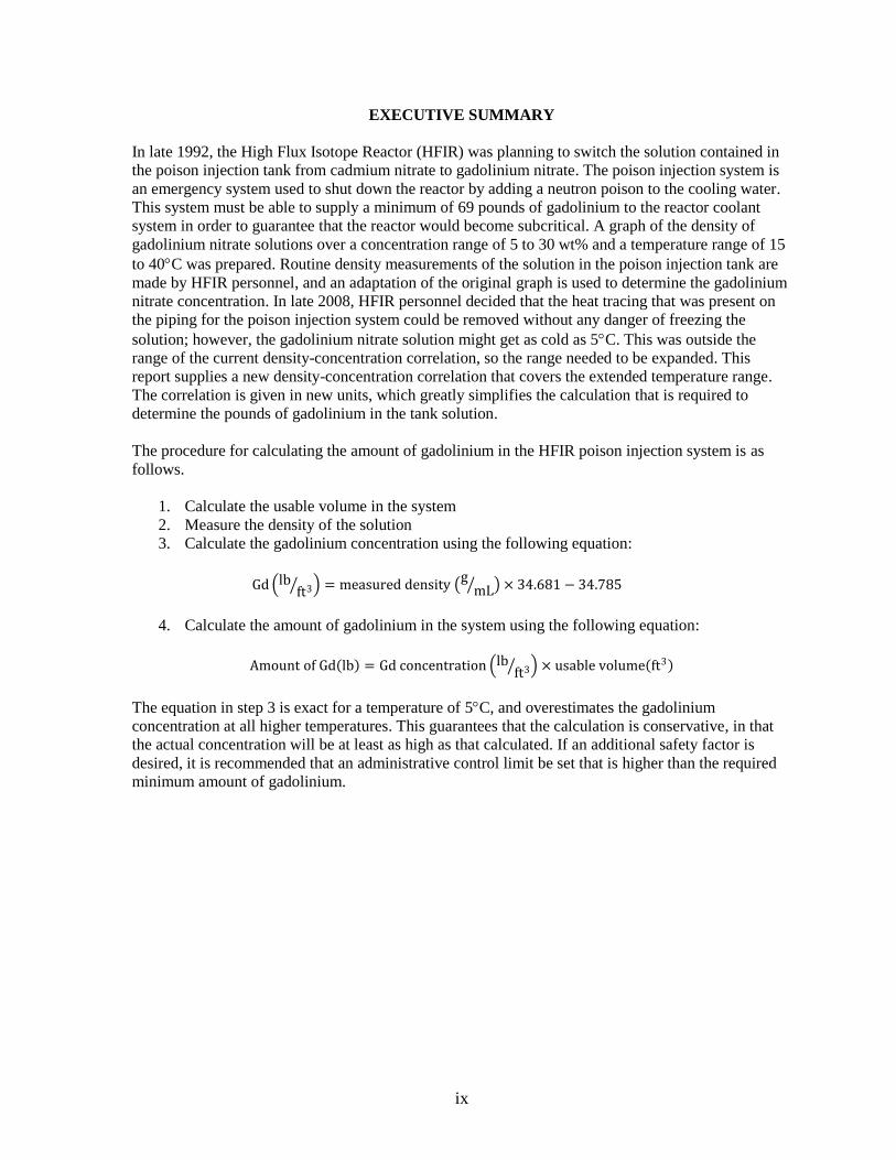
In late 1992, the High Flux Isotope Reactor (HFIR) was planning to switch the solution contained in

the poison injection tank from cadmium nitrate to gadolinium nitrate. The poison injection system is

an emergency system used to shut down the reactor by adding a neutron poison to the cooling water.

This system must be able to supply a minimum of 69 pounds of gadolinium to the reactor coolant

system in order to guarantee that the reactor would become subcritical. A graph of the density of

gadolinium nitrate solutions over a concentration range of 5 to 30 wt% and a temperature range of 15

to 40C was prepared. Routine density measurements of the solution in the poison injection tank are

made by HFIR personnel, and an adaptation of the original graph is used to determine the gadolinium

nitrate concentration. In late 2008, HFIR personnel decided that the heat tracing that was present on

the piping for the poison injection system could be removed without any danger of freezing the

solution; however, the gadolinium nitrate solution might get as cold as 5C. This was outside the

range of the current density-concentration correlation, so the range needed to be expanded. This

report supplies a new density-concentration correlation that covers the extended temperature range.

The correlation is given in new units, which greatly simplifies the calculation that is required to

determine the pounds of gadolinium in the tank solution.

The procedure for calculating the amount of gadolinium in the HFIR poison injection system is as

follows.

1. Calculate the usable volume in the system

2. Measure the density of the solution

3. Calculate the gadolinium concentration using the following equation:

Gd lbft3 = measured density

gmL × 34.681 − 34.785

4. Calculate the amount of gadolinium in the system using the following equation:

Amount of Gd lb = Gd concentration lbft3 × usable volume ft3

The equation in step 3 is exact for a temperature of 5C, and overestimates the gadolinium

concentration at all higher temperatures. This guarantees that the calculation is conservative, in that

the actual concentration will be at least as high as that calculated. If an additional safety factor is

desired, it is recommended that an administrative control limit be set that is higher than the required

minimum amount of gadolinium.

1

1. BACKGROUND

In late 1992 Ken Morgan (Research Reactors Division) asked Paul Taylor (Chemical Technology

Division, currently the Nuclear Science and Technology Division) to supply a graph of the density of

gadolinium nitrate solutions over a concentration range of 5 to 15 wt%, which was later expanded to a

maximum of 30 wt%, and a temperature range of 15 to 40C. The High Flux Isotope Reactor (HFIR)

was planning to switch the solution contained in the poison injection tank from cadmium nitrate to

gadolinium nitrate. The poison injection system is an emergency system that can be used to shut

down the reactor by adding a neutron poison to the cooling water. The density values were obtained

from two published papers.1,2

The first paper had density values for solutions of gadolinium nitrate in

water over the desired range of concentrations, but only at 25C, while the second paper had data for

the density of gadolinium chloride over the desired range of concentrations and temperatures. The

ratio of density change from 25C for each of the desired temperatures at each concentration was

calculated from the gadolinium chloride solution data, and then these ratios were used to calculate the

density of gadolinium nitrate solutions at these conditions by multiplying the density at 25C by the

appropriate ratio.

In late 2008, HFIR personnel decided that the heat tracing that was present on the piping for the

poison injection system could be removed without any danger of freezing the solution; however, the

gadolinium nitrate solution might get as cold as 5C. This was outside the range of the current

density-concentration correlation, so the range needed to be expanded.

The control limits for the gadolinium nitrate solution are based on the total quantity of gadolinium in

the poison injection system tank. Because the density-concentration correlation was given in wt%

gadolinium nitrate, the procedure to calculate the quantity of gadolinium in the tank was much more

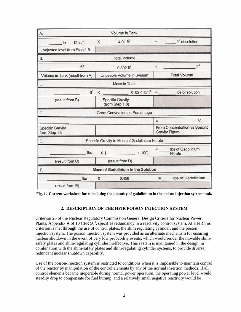
complicated than necessary. A copy of the current calculation worksheet is shown in Fig. 1. The

height of solution in the tank is measured, and then the usable volume of solution is calculated

(steps A and B). These steps would remain the same. A sample of the solution is taken, and the

density (specific gravity) of the solution is measured with a hydrometer. The density-concentration

correlation is used to determine the concentration of gadolinium nitrate, as wt% Gd(NO3)3 in the

solution (step D). The density measurement is also used to calculate the weight of solution, using the

volume of solution that was previously calculated (step C). The amount of gadolinium nitrate is then

calculated from the weight of solution and the wt% Gd(NO3)3 (step E). Finally the weight of

gadolinium is calculated from the weight fraction of gadolinium in Gd(NO3)3 (step F). Many of these

steps could be avoided if the density-concentration correlation were given in units of lb Gd/ft3 vs

density, rather than wt% Gd(NO3)3 vs density.

Section 3 of this report describes the methods for calculating the new concentration-density

correlation and gives the new procedure for calculating the amount of gadolinium in the tank.

2

Fig. 1. Current worksheet for calculating the quantity of gadolinium in the poison injection system tank.

2. DESCRIPTION OF THE HFIR POISON INJECTION SYSTEM

Criterion 26 of the Nuclear Regulatory Commission General Design Criteria for Nuclear Power

Plants, Appendix A of 10 CFR 503, specifies redundancy in a reactivity control system. At HFIR this

criterion is met through the use of control plates, the shim regulating cylinder, and the poison

injection system. The poison injection system was provided as an alternate mechanism for ensuring

nuclear shutdown in the event of very low probability events, which would render the movable shim-

safety plates and shim-regulating cylinder ineffective. This system is maintained in the design, in

combination with the shim-safety plates and shim-regulating cylinder systems, to provide diverse,

redundant nuclear shutdown capability.

Use of the poison-injection system is restricted to conditions when it is impossible to maintain control

of the reactor by manipulation of the control elements by any of the normal insertion methods. If all

control elements became inoperable during normal power operation, the operating power level would

steadily drop to compensate for fuel burnup, and a relatively small negative reactivity would be

3

sufficient to maintain the reactor subcritical following xenon decay. If the control elements should

become inoperable when reactivity is being steadily increased due to xenon burnout following a

scram and restart of the reactor, then (a) sufficient negative reactivity must be available in the poison

injection system to shut down with the control elements fully withdrawn, and (b) the response time of

the poison injection system must be short enough that the reactor can be shut down before the power

is increased to a point that approaches the core thermal limits. This “xenon burnout” scenario was

selected to provide the design basis for the system. The maximum negative reactivity required of the

system was taken as the excess reactivity of a fresh core with control rods fully withdrawn, and the

response time of the system to obtain full injection and mixing of the poison solution was taken as

2½ min. The release of soluble poison into the coolant system within 2½ min of a “servo insert error”

alarm will shut down the reactor without reaching the core thermal limits, assuming the maximum

rate of xenon burnout is consistent with the allowable restart power schedule.

The design of the poison injection system is as follows: The amount of neutron poison available shall

be sufficient, when uniformly distributed in the primary coolant system, to completely poison a clean

core with the control rods fully withdrawn. The neutron poison shall have a chemical form that is

compatible with the materials used in the primary coolant system. The solubility and concentration of

the neutron poison shall be such that it has adequate margin for solution under the normal ambient

conditions present in the poison injection system. The poison injection system must be operable any

time the reactor is operating at power levels greater than 8.5 MW.

The material selected to satisfy these criteria for use in the HFIR poison injection system was

gadolinium nitrate (Gd(NO3)3). The amount of gadolinium material required to maintain subcriticality

under the above conditions was calculated to be a concentration of 0.6 grams gadolinium per liter of

water. This translates to be a minimum of 69 lb of gadolinium (not Gd(NO3)3) dissolved in the HFIR

primary coolant system. The amount of Gd(NO3)3 dissolved in the HFIR poison injection system is

verified monthly.

3. CALCULATION OF DENSITY-CONCENTRATION CORRELATION

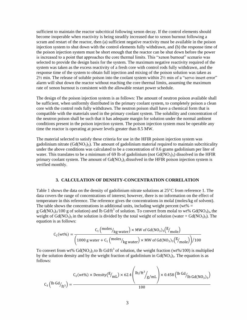
Table 1 shows the data on the density of gadolinium nitrate solutions at 25C from reference 1. The

data covers the range of concentrations of interest; however, there is no information on the effect of

temperature in this reference. The reference gives the concentrations in molal (moles/kg of solvent).

The table shows the concentrations in additional units, including weight percent (wt% =

g Gd(NO3)3/100 g of solution) and lb Gd/ft3 of solution. To convert from molal to wt% Gd(NO3)3, the

weight of Gd(NO3)3 in the solution is divided by the total weight of solution (water + Gd(NO3)3). The

equation is as follows:

C2 wt% =C1

moleskg water × MW of Gd NO3 3

gmole

1000 g water + C1 moles

kg water × MW of Gd NO3 3 g

mole 100

To convert from wt% Gd(NO3)3 to lb Gd/ft3 of solution, the weight fraction (wt%/100) is multiplied

by the solution density and by the weight fraction of gadolinium in Gd(NO3)3. The equation is as

follows:

C3 lb Gd

ft3 =

C2 wt% × Density g

mL × 62.4 lb ft3 g mL × 0.458 lb Gd

lb Gd NO3 3

100

4

Table 1. Density of gadolinium nitrate–water solutions at 25C1

Gd(NO3)3 concentrations Gd conc.

(lb Gd/ft3)

Density

(g/mL) (molal) (wt%)

0.1532 4.996 1.486 1.0409

0.2068 6.628 2.000 1.0559

0.2947 9.187 2.836 1.0802

0.4092 12.316 3.912 1.1113

0.5991 17.057 5.662 1.1615

0.7955 21.449 7.428 1.2118

1.0108 25.759 9.311 1.2648

1.2150 29.431 11.048 1.3135

Data on the density variation at various temperatures for gadolinium nitrate solutions was not

available when the initial density calibration was done; therefore, published data for gadolinium

chloride solutions2 was used to estimate the density of gadolinium nitrate solutions at various

temperatures. Table 2 shows the data from reference 2, which is in the form of coefficients for a

power function equation.

Table 2. Coefficients for power function equation to calculate gadolinium

chloride solution densitiesa

[Gd Cl3]

(molal) C0 C1 C2 C3 C4 C5

0.0978 1.0243 2.758E-05 –7.673E-06 5.884E-08 –3.832E-10 1.1630E-12

0.2368 1.0584 –1.761E-05 –6.806E-06 4.859E-08 –3.045E-10 8.9523E-13

0.4105 1.1002 –7.157E-05 –5.777E-06 3.618E-08 –2.075E-10 5.6368E-13

0.5894 1.1423 –1.197E-04 –4.996E-06 2.863E-08 –1.584E-10 4.1682E-13

0.7842 1.1874 –1.696E-04 –4.151E-06 1.917E-08 –8.740E-11 1.8198E-13

0.9947 1.2349 –2.147E-04 –3.565E-06 1.518E-08 –7.142E-11 1.5841E-13

1.2239 1.2854 –2.600E-04 –3.038E-06 1.258E-08 –7.384E-11 2.2978E-13 aAdapted from Habenschuss and Spedding2

Note: Density = Co + C1(T) + C2(T)2 + C3(T)3 + C4(T)4 + C5(T)5, where T = Temperature (oC).

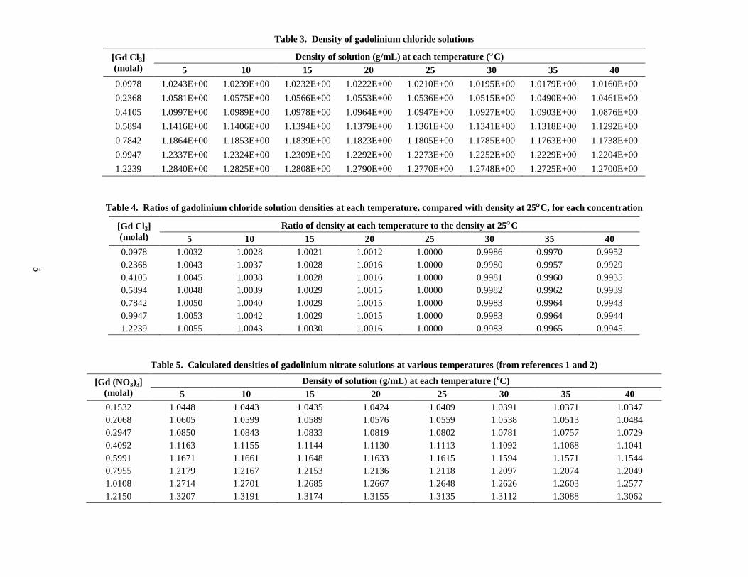
Table 3 shows the densities of gadolinium chloride solutions at various concentrations and

temperatures, which were calculated from the equation and coefficients listed above. Table 4 shows

the ratio of the density at each temperature to the density at 25C at each concentration. These ratios

were used to calculate the density of the gadolinium nitrate solutions at various temperatures, from

the published densities at 25C. The maximum difference between the densities at 5C and 40C was

1.1%, which occurred at the highest gadolinium chloride concentration, so temperature within this

range has a relatively small effect on the density of the solutions. Since the density variation with

temperature is small, and gadolinium nitrate and gadolinium chloride solutions should have similar

temperature dependencies, using the measured gadolinium chloride temperature dependency to

predict the temperature dependency is justified.

Table 5 shows the calculated densities for gadolinium nitrate solutions at various temperatures. The

values were calculated from the published densities at 25C, shown in Table 1, and the ratios shown

5

Table 3. Density of gadolinium chloride solutions

[Gd Cl3]

(molal)

Density of solution (g/mL) at each temperature (C)

5 10 15 20 25 30 35 40

0.0978 1.0243E+00 1.0239E+00 1.0232E+00 1.0222E+00 1.0210E+00 1.0195E+00 1.0179E+00 1.0160E+00

0.2368 1.0581E+00 1.0575E+00 1.0566E+00 1.0553E+00 1.0536E+00 1.0515E+00 1.0490E+00 1.0461E+00

0.4105 1.0997E+00 1.0989E+00 1.0978E+00 1.0964E+00 1.0947E+00 1.0927E+00 1.0903E+00 1.0876E+00

0.5894 1.1416E+00 1.1406E+00 1.1394E+00 1.1379E+00 1.1361E+00 1.1341E+00 1.1318E+00 1.1292E+00

0.7842 1.1864E+00 1.1853E+00 1.1839E+00 1.1823E+00 1.1805E+00 1.1785E+00 1.1763E+00 1.1738E+00

0.9947 1.2337E+00 1.2324E+00 1.2309E+00 1.2292E+00 1.2273E+00 1.2252E+00 1.2229E+00 1.2204E+00

1.2239 1.2840E+00 1.2825E+00 1.2808E+00 1.2790E+00 1.2770E+00 1.2748E+00 1.2725E+00 1.2700E+00

Table 4. Ratios of gadolinium chloride solution densities at each temperature, compared with density at 25C, for each concentration

[Gd Cl3]

(molal)

Ratio of density at each temperature to the density at 25C

5 10 15 20 25 30 35 40

0.0978 1.0032 1.0028 1.0021 1.0012 1.0000 0.9986 0.9970 0.9952

0.2368 1.0043 1.0037 1.0028 1.0016 1.0000 0.9980 0.9957 0.9929

0.4105 1.0045 1.0038 1.0028 1.0016 1.0000 0.9981 0.9960 0.9935

0.5894 1.0048 1.0039 1.0029 1.0015 1.0000 0.9982 0.9962 0.9939

0.7842 1.0050 1.0040 1.0029 1.0015 1.0000 0.9983 0.9964 0.9943

0.9947 1.0053 1.0042 1.0029 1.0015 1.0000 0.9983 0.9964 0.9944

1.2239 1.0055 1.0043 1.0030 1.0016 1.0000 0.9983 0.9965 0.9945

Table 5. Calculated densities of gadolinium nitrate solutions at various temperatures (from references 1 and 2)

[Gd (NO3)3]

(molal)

Density of solution (g/mL) at each temperature (oC)

5 10 15 20 25 30 35 40

0.1532 1.0448 1.0443 1.0435 1.0424 1.0409 1.0391 1.0371 1.0347

0.2068 1.0605 1.0599 1.0589 1.0576 1.0559 1.0538 1.0513 1.0484

0.2947 1.0850 1.0843 1.0833 1.0819 1.0802 1.0781 1.0757 1.0729

0.4092 1.1163 1.1155 1.1144 1.1130 1.1113 1.1092 1.1068 1.1041

0.5991 1.1671 1.1661 1.1648 1.1633 1.1615 1.1594 1.1571 1.1544

0.7955 1.2179 1.2167 1.2153 1.2136 1.2118 1.2097 1.2074 1.2049

1.0108 1.2714 1.2701 1.2685 1.2667 1.2648 1.2626 1.2603 1.2577

1.2150 1.3207 1.3191 1.3174 1.3155 1.3135 1.3112 1.3088 1.3062

6

in Table 4. Where the gadolinium chloride concentrations were close to the gadolinium nitrate

concentrations, the ratios in Table 4 were used directly; otherwise, interpolated values were used to

calculate the densities of the gadolinium nitrate solutions.

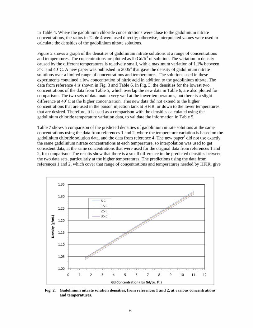
Figure 2 shows a graph of the densities of gadolinium nitrate solutions at a range of concentrations

and temperatures. The concentrations are plotted as lb Gd/ft3 of solution. The variation in density

caused by the different temperatures is relatively small, with a maximum variation of 1.1% between

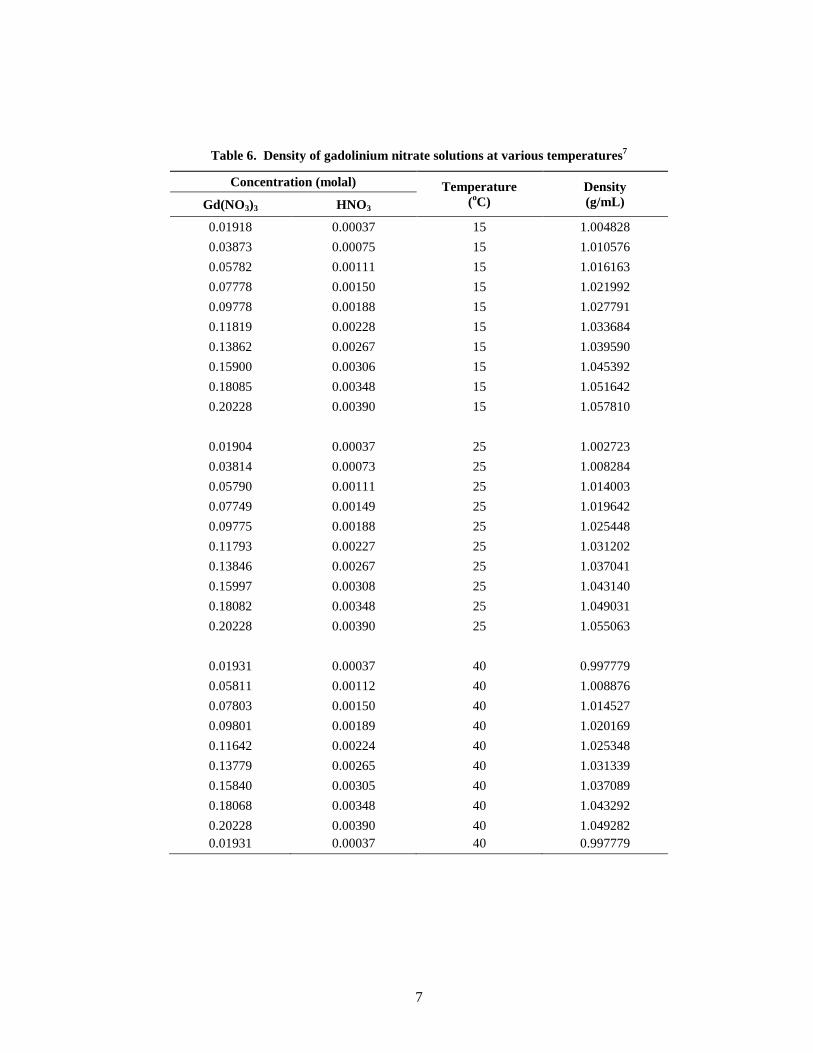
5C and 40C. A new paper was published in 20054 that gave the density of gadolinium nitrate

solutions over a limited range of concentrations and temperatures. The solutions used in these

experiments contained a low concentration of nitric acid in addition to the gadolinium nitrate. The

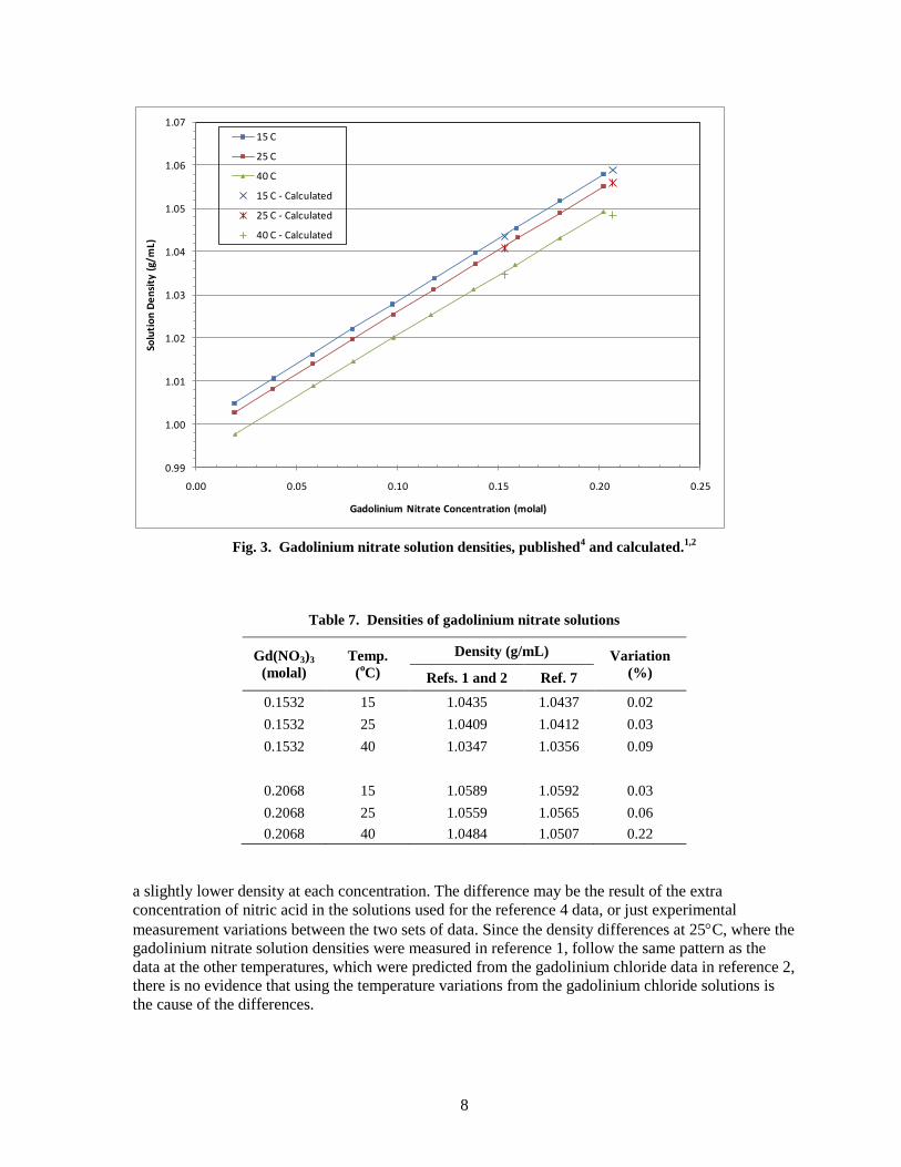
data from reference 4 is shown in Fig. 3 and Table 6. In Fig. 3, the densities for the lowest two

concentrations of the data from Table 5, which overlap the new data in Table 6, are also plotted for

comparison. The two sets of data match very well at the lower temperatures, but there is a slight

difference at 40C at the higher concentration. This new data did not extend to the higher

concentrations that are used in the poison injection tank at HFIR, or down to the lower temperatures

that are desired. Therefore, it is used as a comparison with the densities calculated using the

gadolinium chloride temperature variation data, to validate the information in Table 5.

Table 7 shows a comparison of the predicted densities of gadolinium nitrate solutions at the same

concentrations using the data from references 1 and 2, where the temperature variation is based on the

gadolinium chloride solution data, and the data from reference 4. The new paper4 did not use exactly

the same gadolinium nitrate concentrations at each temperature, so interpolation was used to get

consistent data, at the same concentrations that were used for the original data from references 1 and

2, for comparison. The results show that there is a small difference in the predicted densities between

the two data sets, particularly at the higher temperatures. The predictions using the data from

references 1 and 2, which cover that range of concentrations and temperatures needed by HFIR, give

Fig. 2. Gadolinium nitrate solution densities, from references 1 and 2, at various concentrations

and temperatures.

1.00

1.05

1.10

1.15

1.20

1.25

1.30

1.35

0 1 2 3 4 5 6 7 8 9 10 11 12

De

nsi

ty (

g/m

L)

Gd Concentration (lbs Gd/cu. ft.)

5 C

15 C

25 C

35 C

7

Table 6. Density of gadolinium nitrate solutions at various temperatures7

Concentration (molal) Temperature

(oC)

Density

(g/mL) Gd(NO3)3 HNO3

0.01918 0.00037 15 1.004828

0.03873 0.00075 15 1.010576

0.05782 0.00111 15 1.016163

0.07778 0.00150 15 1.021992

0.09778 0.00188 15 1.027791

0.11819 0.00228 15 1.033684

0.13862 0.00267 15 1.039590

0.15900 0.00306 15 1.045392

0.18085 0.00348 15 1.051642

0.20228 0.00390 15 1.057810

0.01904 0.00037 25 1.002723

0.03814 0.00073 25 1.008284

0.05790 0.00111 25 1.014003

0.07749 0.00149 25 1.019642

0.09775 0.00188 25 1.025448

0.11793 0.00227 25 1.031202

0.13846 0.00267 25 1.037041

0.15997 0.00308 25 1.043140

0.18082 0.00348 25 1.049031

0.20228 0.00390 25 1.055063

0.01931 0.00037 40 0.997779

0.05811 0.00112 40 1.008876

0.07803 0.00150 40 1.014527

0.09801 0.00189 40 1.020169

0.11642 0.00224 40 1.025348

0.13779 0.00265 40 1.031339

0.15840 0.00305 40 1.037089

0.18068 0.00348 40 1.043292

0.20228 0.00390 40 1.049282

0.01931 0.00037 40 0.997779

8

Fig. 3. Gadolinium nitrate solution densities, published4 and calculated.

1,2

Table 7. Densities of gadolinium nitrate solutions

Gd(NO3)3

(molal)

Temp.

(oC)

Density (g/mL) Variation

(%) Refs. 1 and 2 Ref. 7

0.1532 15 1.0435 1.0437 0.02

0.1532 25 1.0409 1.0412 0.03

0.1532 40 1.0347 1.0356 0.09

0.2068 15 1.0589 1.0592 0.03

0.2068 25 1.0559 1.0565 0.06

0.2068 40 1.0484 1.0507 0.22

a slightly lower density at each concentration. The difference may be the result of the extra

concentration of nitric acid in the solutions used for the reference 4 data, or just experimental

measurement variations between the two sets of data. Since the density differences at 25C, where the

gadolinium nitrate solution densities were measured in reference 1, follow the same pattern as the

data at the other temperatures, which were predicted from the gadolinium chloride data in reference 2,

there is no evidence that using the temperature variations from the gadolinium chloride solutions is

the cause of the differences.

0.99

1.00

1.01

1.02

1.03

1.04

1.05

1.06

1.07

0.00 0.05 0.10 0.15 0.20 0.25

Solu

tio

n D

en

sity

(g/

mL)

Gadolinium Nitrate Concentration (molal)

15 C

25 C

40 C

15 C - Calculated

25 C - Calculated

40 C - Calculated

9

The reference 4 data gives slightly higher gadolinium nitrate concentrations than the reference 1 and 2

data at each temperature and concentration. For a given measured density, the correlation from the

reference 1 and 2 data (Table 5 and Fig. 2) would predict a lower gadolinium nitrate concentration

than the reference 4 data. Therefore, using the correlation from the reference 1 and 2 data would give

the lowest predicted gadolinium concentration for a given density measurement for the solution in the

HFIR poison injection system, which would be conservative for the HFIR application and guarantee

that the actual amount of gadolinium in the system is not less than that calculated.

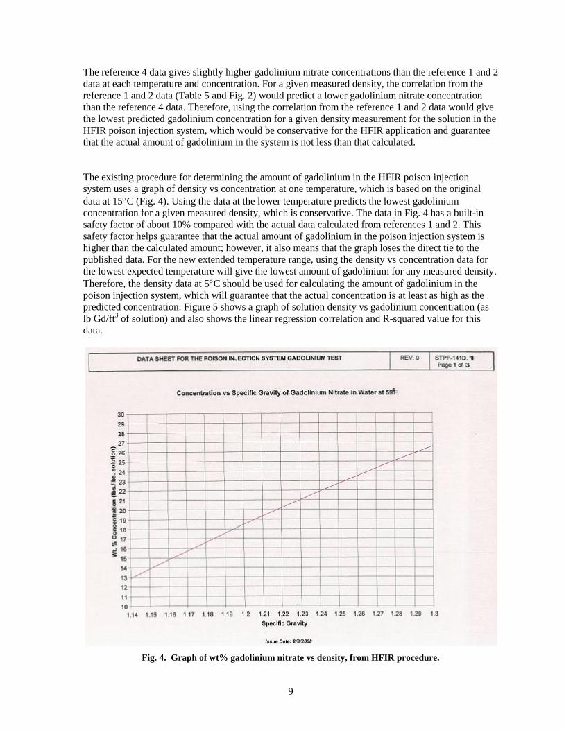
The existing procedure for determining the amount of gadolinium in the HFIR poison injection

system uses a graph of density vs concentration at one temperature, which is based on the original

data at 15C (Fig. 4). Using the data at the lower temperature predicts the lowest gadolinium

concentration for a given measured density, which is conservative. The data in Fig. 4 has a built-in

safety factor of about 10% compared with the actual data calculated from references 1 and 2. This

safety factor helps guarantee that the actual amount of gadolinium in the poison injection system is

higher than the calculated amount; however, it also means that the graph loses the direct tie to the

published data. For the new extended temperature range, using the density vs concentration data for

the lowest expected temperature will give the lowest amount of gadolinium for any measured density.

Therefore, the density data at 5C should be used for calculating the amount of gadolinium in the

poison injection system, which will guarantee that the actual concentration is at least as high as the

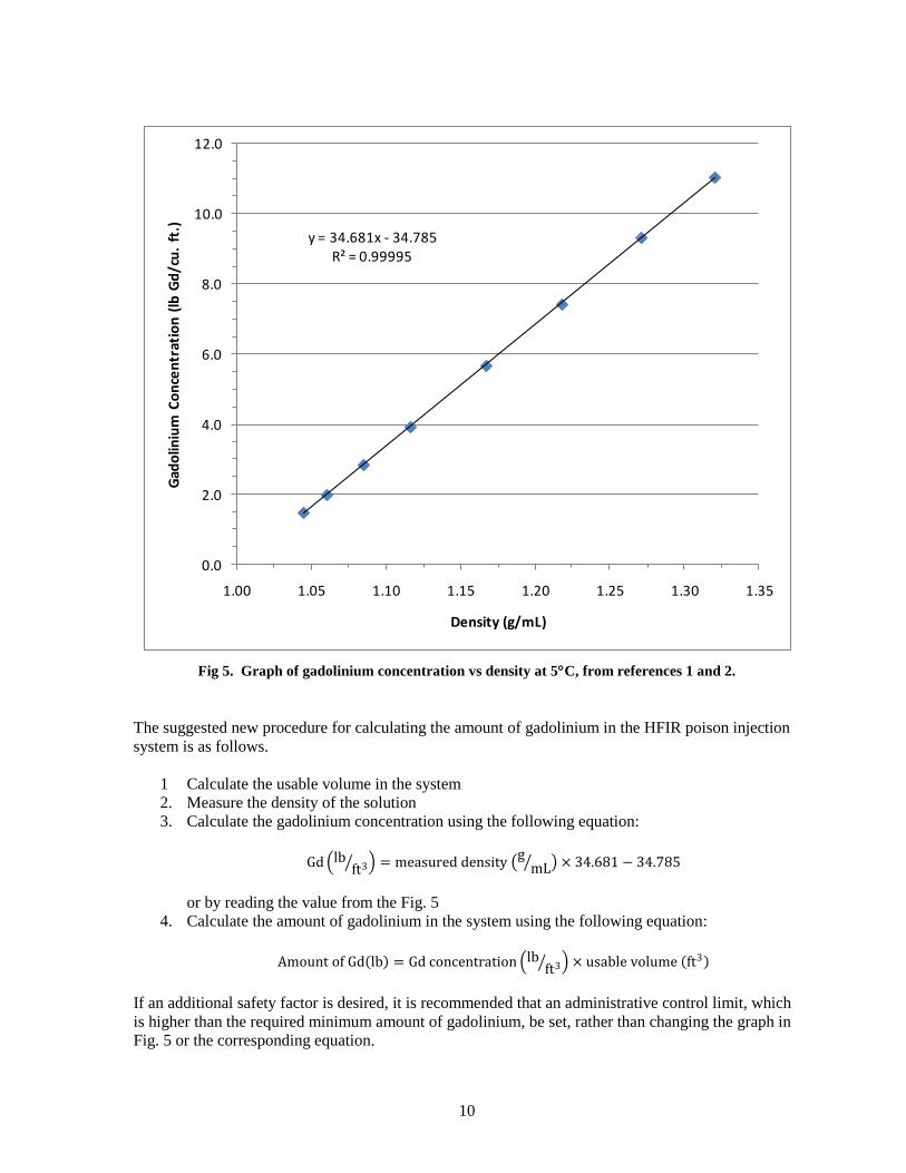
predicted concentration. Figure 5 shows a graph of solution density vs gadolinium concentration (as

lb Gd/ft3 of solution) and also shows the linear regression correlation and R-squared value for this

data.

Fig. 4. Graph of wt% gadolinium nitrate vs density, from HFIR procedure.

10

Fig 5. Graph of gadolinium concentration vs density at 5C, from references 1 and 2.

The suggested new procedure for calculating the amount of gadolinium in the HFIR poison injection

system is as follows.

1 Calculate the usable volume in the system

2. Measure the density of the solution

3. Calculate the gadolinium concentration using the following equation:

Gd lbft3 = measured density

gmL × 34.681 − 34.785

or by reading the value from the Fig. 5

4. Calculate the amount of gadolinium in the system using the following equation:

Amount of Gd lb = Gd concentration lbft3 × usable volume ft3

If an additional safety factor is desired, it is recommended that an administrative control limit, which

is higher than the required minimum amount of gadolinium, be set, rather than changing the graph in

Fig. 5 or the corresponding equation.

y = 34.681x - 34.785R² = 0.99995

0.0

2.0

4.0

6.0

8.0

10.0

12.0

1.00 1.05 1.10 1.15 1.20 1.25 1.30 1.35

Gad

olin

ium

Co

nce

ntr

atio

n (

lb G

d/c

u.

ft.)

Density (g/mL)

11

For a typical density of 1.2 g/mL in the poison injection system, the equation above would give a

gadolinium concentration of 6.83 lb/ft3. The graph in the HFIR procedure would give a concentration

of 18.5 wt% = 6.24 lb Gd/ft3. Because of the safety factor built into the old graph, this result is about

8% lower than the actual concentration.

13

4. REFERENCES

1. F. H. Spedding et al., “Densities and Apparent Molal Volumes of Some Aqueous Rare Earth

Solutions at 25C,” J. of Physical Chemistry 79(11), 1087–1096 (1975).

2. A. Habenschuss and F. Spedding, “Densities and Thermal Expansion of Some Aqueous Rare

Earth Chloride Solutions Between 5 and 80C. II. SmCl3, GdCl3, DyCl3, ErCl3, and YbCl3,” J. of

Chemical & Engineering Data 21(1), 95–113 (1976).

3. General Design Criteria for Nuclear Power Plants, Appendix A, 10 CFR 50, U.S. Nuclear

Regulatory Commission.

4. A. W. Hakin, J. L. Liu, K. Erickson, J.-V.Munoz, and J. A. Rard, “Apparent molar volumes

and apparent molar heat capacities of Pr(NO3)3(aq), Gd(NO3)3(aq), Ho(NO3)3(aq), and Y(NO3)3(aq) at

T = (288.15, 298.15, 313.15, and 328.15) K and p = 0.1 Mpa,” J. Chem. Thermodynamics 37,

153–167 (2005).

ORNL/TM-2009/091

INTERNAL DISTRIBUTION

1. D. L. Pinkston 4. P. A. Taylor

2. A. H. Primm 5. ORNL Office of Technical Information

3. D. L. Schuh and Classification