M.I.E.T. ENGINEERING COLLEGE

(Approved by AICTE and Affiliated to Anna University Chennai)

TRICHY – PUDUKKOTTAI ROAD, TIRUCHIRAPPALLI – 620 007

DEPARTMENT OF COMPUTER SCIENCE AND ENGINEERING

COURSE MATERIAL

IT6601 - DATAWAREHOUSING

&

DATA MINING

M.I.E.T. ENGINEERING COLLEGE

(Approved by AICTE and Affiliated to Anna University Chennai)

TRICHY – PUDUKKOTTAI ROAD, TIRUCHIRAPPALLI – 620 007

DEPARTMENT OF COMPUTER SCIENCE & ENGINEERING

COURSE OBJECTIVE

1. To understand the basic concepts,functions of OS .

2. Learn about process,threads & scheduling algorithms.

3. Understand the principles of concurrency & deadlock. 4. Learn various memory management schemes.

5. Learn the basics of Linux systems & mobile OS.

COURSE OUTCOMES

1. Understand the basic concepts and functions of Operating Systems

2. Delineate various threading models, process synchronization and deadlocks

3. Compare the performance of various CPU scheduling algorithms 4. Understand the basic concepts of memory management systems

5. Expound I/O management and file systems

6. Understand the model of Linux multifunction server and utilize local network services

Prepared by Verified By

STAFF NAME HOD

Approved by

PRINCIPAL

Sub. Code : IT6702 Branch/Year/Sem : CSE/III/VI

Sub Name : DATAWAREHOUSING & DATA MINING Batch :

Staff Name :S.SHANMUGA PRIYA Academic Year :

M.I.E.T. ENGINEERING COLLEGE

(Approved by AICTE and Affiliated to Anna University Chennai)

TRICHY – PUDUKKOTTAI ROAD, TIRUCHIRAPPALLI – 620 007

DEPARTMENT OF COMPUTER SCIENCE & ENGINEERING

SYLLABUS (THEORY)

Sub. Code : IT6702 Branch / Year / Sem : CSE/III/VI

Sub. Name : Data warehousing & Data mining Batch :

Staff Name : S.SHANMUGA PRIYA Academic Year :

L T P C

3 0 0 3

UNIT I DATA WAREHOUSING 9

Data warehousing Components –Building a Data warehouse –- Mapping the Data Warehouse to a

Multiprocessor Architecture – DBMS Schemas for Decision Support – Data Extraction, Cleanup, and

Transformation Tools –Metadata.

UNIT II BUSINESS ANALYSIS 9

Reporting and Query tools and Applications – Tool Categories – The Need for Applications – Cognos

Impromptu – Online Analytical Processing (OLAP) – Need – Multidimensional Data Model – OLAP

Guidelines – Multidimensional versus Multi relational OLAP – Categories of Tools – OLAP Tools and the

Internet.

UNIT III DATA MINING 9

Introduction – Data – Types of Data – Data Mining Functionalities – Interestingness of Patterns – Classification

of Data Mining Systems – Data Mining Task Primitives – Integration of a Data Mining System with a Data

Warehouse – Issues –Data Preprocessing.

UNIT IV ASSOCIATION RULE MINING AND CLASSIFICATION 9

Mining Frequent Patterns, Associations and Correlations – Mining Methods – Mining various Kinds of

Association Rules – Correlation Analysis – Constraint Based Association Mining – Classification and

Prediction - Basic Concepts - Decision Tree Induction - Bayesian Classification – Rule Based

Classification – Classification by Back propagation – Support Vector Machines – Associative

Classification – Lazy Learners – Other Classification Methods – Prediction.

UNIT V CLUSTERING AND TRENDS IN DATA MINING 9

Cluster Analysis - Types of Data – Categorization of Major Clustering Methods – K-means– Partitioning

Methods – Hierarchical Methods - Density-Based Methods –Grid Based Methods – Model-Based

Clustering Methods – Clustering High Dimensional Data - Constraint – Based Cluster Analysis – Outlier

Analysis – Data Mining Applications.

TOTAL: 45 PERIODS

TEXT BOOKS:

な. Alex Berson and Stephen J.Smith, ╉Data Warehousing, Data Mining and OLAP╊, Tata McGraw

– Hill Edition, Thirteenth Reprint 2008.

に. Jiawei Han and Micheline Kamber, ╉Data Mining Concepts and Techniques╊, Third Edition,

Elsevier, 2012.

REFERENCES:

1. Pang-Ning Tan, Michael Steinbach and Vipin Kumar, ╉Introduction to DataMining╊, Person Education, 2007.

に. K.P. Soman, Shyam Diwakar and V. Aja, ╉Insight into Data Mining Theory and Practice╊, Eastern

Economy Edition, Prentice Hall of India, 2006.

ぬ. G. K. Gupta, ╉Introduction to Data Mining with Case Studies╊, Eastern Economy Edition, Prentice

Hall of India, 2006.

ね. Daniel T.Larose, ╉Data Mining Methods and Models╊, Wiley-Interscience, 2006.

UNIT - I DATA WAREHOUSING

Data warehousing Components –Building a Data warehouse –- Mapping the Data Warehouse

to a Multiprocessor Architecture – DBMS Schemas for Decision Support – Data Extraction, Cleanup,

and Transformation Tools –Metadata.

Data Warehouse

A data warehouse is a collection of data marts representing historical data from different

operations in the company.

It collect the data from multiple heterogeneous data base files (flat, text and etc).

It store the5 to 10years of huge amount of data.

This data is stored in a structure optimized for querying and data analysis as a data

warehouse.

A warehouse is a subject-oriented, integrated, time-variant and non-volatile collection of data in

support of management’s decision making process‖.

Subject Oriented: Data that gives information about a particular subject instead of about a

company’s ongoing operations.

Integrated: Data that is gathered into the data warehouse from a variety of sources and merged into a

coherent whole.

Time-variant : All data in the data warehouse is identified with a particular time period.

Non-volatile: Data is stable in a data warehouse. More data is added but data is never removed.

It can be Used for decision Support

Used to manage and control business

Used by managers and end-users to understand the business and make judgments

Other important terminology

Enterprise Data warehouse: It collects all information about subjects (customers, products, sales,

assets, personnel) that span the entire organization

Decision Support System (DSS): Information technology to help the knowledge worker (executive,

manager, and analyst) makes faster & better decisions.

Operational and informational Data

Operation al Data:

Focusing on transactional function such as bank card withdrawals and deposits

Detailed

Updateable

Reflects current data

Information al Data:

Focusing on providing answers to problems posed by decision makers

Summarized

Non updateable

Data Warehouse Characteristics

It is a database designed for analytical tasks

Its content is periodically updated

It contains current and historical data to provide historical perspective of information.

1.1 DATA WAREHOUSECOMPONENTS

Overall Architecture

The data warehouse architecture is based on the data base management system server.

The central information repository is surrounded by number of key components

Data warehouse is an environment, not a product which is based on relational database

management system that functions as the central repository for informational data.

The data entered into the data warehouse transformed into an integrated structure and

format. The transformation process involves conversion, summarization, filtering and

condensation.

The data warehouse must be capable of holding and managing large volumes of data as

well as different structure of data structures over the time.

Key components

Data sourcing, cleanup, transformation, and migration tools

Metadata repository

Warehouse/database technology

Data marts

Data query, reporting, analysis, and mining tools

Data warehouse administration and management

Information delivery system

1.1.1 Data sourcing, cleanup, transformation, and migration tools

They perform conversions, summarization, key changes, structural changes

The data transformation is required to use by decision support tools.

The transformation produces programs, control statements.

It moves the data into data warehouse from multiple operational systems. The

Functionalities of these tools are listed below:

To remove unwanted data from operational db

Converting to common data names and attributes

Calculating summaries and derived data

Establishing defaults for missing data

Accommodating source data definition changes

1.1.2. Metadata repository

It is data about data. It is used for maintaining, managing and using the data warehouse. It is

classified into two:

Technical Meta data: It contains information about data warehouse data used by warehouse designer,

administrator to carry out development and management tasks. It includes,

Info about data stores.

Transformation descriptions. That si mapping methods from operational db to warehouse db.

Warehouse Object and data structure definitions for target data

The rules used to perform clean up, and data enhancement

Data mapping operations

Access authorization, backup history, archive history, info delivery history, data acquisition

history, data access etc.,

Business Meta data: It contains info that gives info stored in data warehouse to users. It includes,

Subject areas, and info object type including queries, reports, images, video, audio clips etc.

Internet home pages

Info related to info delivery system

Data warehouse operational info such as ownerships, audit trails etc. ,

Meta data helps the users to understand content and find the data. Meta data are stored in a

separate data stores which is known as informational directory or Meta data repository which

helps to integrate, maintain and view the contents of the data warehouse.

The following lists the characteristics of info directory/ Meta data:

It is the gateway to the data warehouse environment

It supports easy distribution and replication of content for high performance and availability

It should be searchable by business oriented key words

It should act as a launch platform for end user to access data and analysis tools

It should support the sharing of info

It should support scheduling options for request

It should support and provide interface to other applications

It should support end user monitoring of the status of the data warehouse environment

1.1.3Warehouse/database technology

Data ware house database

This is the central part of the data ware housing environment. This is implemented based on

RDBMS technology.

1.1.4 Data marts It is inexpensive tool and alternative to the data ware house. it based on the subject area Data mart is

used in the following situation:

Extremely urgent user requirement

The absence of a budget for a full scale data warehouse strategy

The decentralization of business needs

1.1.5 Data query, reporting ,analysis, and mining tools

Its purpose is to provide info to business users for decision making. There are five

categories:

Data query and reporting tools

Application development tools

Executive info system tools (EIS)

OLAP tools

Data mining tools

Query and reporting tools:

Used to generate query and report. There are two types of reporting tools. They are:

Production reporting tool used to generate regular operational reports

Desktop report writer are inexpensive desktop tools designed for end users.

Managed Query tools: used to generate SQLquery. It uses Met layer software in between users and

databases which offers appoint-and-click creation of SQL statement.

Application development tools: This is a graphical data access environment which integrates OLAP

tools with data warehouse and can be used to access all db systems.

OLAP Tools: Are used to analyze the data in multidimensional and complex views.

Data mining tools: Are used to discover knowledge from the data warehouse data.

1.1.6.Data ware house administration and management

The management of data warehouse includes,

Security and priority management

Monitoring updates from multiple sources

Data quality checks

Managing and updating meta data

Auditing and reporting data warehouse usage and status

Purging data

Replicating, sub setting and distributing data

Backup and recovery

Data warehouse storage management which includes capacity planning, hierarchical storage

management and purging of aged data etc.,

1.1.7. Information delivery system

It is used to enable the process of subscribing for data warehouse info.

Delivery to one or more destinations according to specified scheduling algorithm

1.2 BUILDING A DATA WAREHOU SE

There are two reasons why organizations consider data warehousing a critical need. In other

words, there are two factors that drive you to build and use data warehouse. They are:

Business factors:

Business users want to make decision quickly and correctly using all available data.

Technological factors:

To address the incompatibility of operational data stores

IT infrastructure is changing rapidly. Its capacity is increasing and cost is decreasing so that

building a data warehouse is easy.

1.2.1 Business factors

Business considerations:

Two approaches:

Top– Down Approach

Bottom– Up Approach

Top – Down Approach

It collected enterprise wide business requirements and decided to build an enterprise data warehouse

with subset data marts.

Bottom Up Approach

The data marts are integrated or combined together to form a data warehouse.

The bottom up approach helps us incrementally build the warehouse by developing and

integrating data marts as and when the requirements are clear.

The advantage of using the Bottom Up approach is that they do not require high initial

costs and have a faster implementation time;

Bottom up approach is more realistic but the complexity of the integration may become

a serious obstacle.

Design considerations:

In general a data warehouse data from multiple heterogeneous sources into a query database

this is also one of the reasons why a data warehouse is difficult to built

Data content

The content and structure of the data warehouse are reflected in its data model.

The data model is the template that describes how information will be organized

within the integrated warehouse framework.

The data warehouse data must be a detailed data. It must be formatted, cleaned up and

Transformed to fit the warehouse data model.

Meta data

It defines the location and contents of data in the warehouse.

Meta data is searchable by users to find definitions or subject areas.

Data distribution

Data volumes continue to grow in nature. Therefore, it becomes necessary to know how

the data should be divided across multiple servers.

The data can be distributed based on the subject area, location (geographical region),

or time (current, month, year).

Tools

A number of tools are available that are specifically designed to help in the

implementation of the data warehouse.

These tools for defining a cleanup, data movement, end user, query, reporting and

data analysis.

Performance considerations

The actual performance levels are dependent and vary widely from one environment to

another. it is relatively difficult to predict the performance of a typical data warehouse.

The following nine-step method is followed in the design of a data warehouse:

1. Choosing the subject matter

2. Deciding what a fact table represents

3. Identifying and conforming the dimensions

4. Choosing the facts

5. Storing pre calculations in the fact table

6. Rounding out the dimension table

7. Choosing the duration of the db

8. The need to track slowly changing dimensions

9. Deciding the query priorities and query Models.

1.2.2 Technological factors

Technical considerations:

Hardware platforms

An important consideration when choosing a data warehouse server capacity for

handling the high volumes of data.

It has large data and through put.

The modern server can also support large volumes and large number of flexible GUI

Data warehouse and DBMS specialization

Very large size of databases and need to process complex adhoc queries in a short time

The most important requirements for the data warehouse DBMS are performance,

throughput and scalability.

Communication infrastructure

The data warehouse user requires a relatively large band width to interact with the data

warehouse and retrieve a significant amount of data for analysis.

This may mean that communication networks have to be expanded and new hardware

and software may have purchased.

Implementation considerations

Collect and analyze business requirements

Create a data model

Define data sources

Choose a data base technology

Choose database access and reporting tools

Choose database connectivity s/w

Choose analysis and presentation s/w

Access tools:

Data warehouse implementation relies on selecting suitable data access tools.

The following lists the various type of data that can be accessed:

Simple tabular form data

Ranking data

Multivariable data

Time series data

Graphing, charting and pivoting data

Data extraction, clean up, transformation and migration:

Timeliness of data delivery to the warehouse

The tool must have the ability to identify the particular data and that can be read by

conversion tool.

The tool must support flat files, indexed files since corporate data is still in this type

The tool must have the capability to merge data from multiple data stores

The tool should have specification interface to indicate the data to be extracted

The tool should have the ability to read data from data dictionary

The code generated by the tool should be completely maintainable

The data warehouse database system must be able to perform loading data directly from

these tools.

Data replication

Data replication or data moves to place the data to a particular workgroup in a localized

database.

Most companies use data replication servers to copy their most needed data to a

separate database.

Metadata

It is a road map to the information stores in the warehouse is metadata it defines all elements

and their attributes.

Data placement strategies

As a data warehouse grows, there are at least two options for data placement. One is to put

some of the data in the data warehouse into another storage media.

The second option is to distribute the data in the data warehouse across multiple servers.

User levels

The users of data warehouse data can be classified on the basis of their skill level in accessing

the warehouse. There are three classes of users:

Casual users: are most comfortable in retrieving info from warehouse in pre defined

formats and running pre existing queries and reports.

Power Users: can use pre defined as well as user defined queries to create simple and ad

hoc reports. These users can engage in drill down operations. These users may have the

experience of using reporting and query tools.

Expert users: These users tend to create their own complex queries and perform standard

analysis on the info they retrieve. These users have the knowledge about the use of query and

report tools

Benefits of data warehousing

The benefits can be classified into two:

Tangible benefits (quantified / measureable):It includes,

Improvement in product inventory

Decrement in production cost

Improvement in selection of target markets

Enhancement in asset and liability management

Benefits Intangible (not easy to quantified): It includes,

Improvement in productivity by keeping all data in single location and eliminating rekeying of

data.

Reduced redundant processing Enhanced customer relation.

1.3 MAPPING THEDATA WA REHOUSEARCHIT ECTURE TO MULTI PROCESSOR

ARCHIT ECTURE

1.3.1. Relational data base technology for data warehouse

Linear Speed up: refers the ability to increase the number of processor to reduce response time

Linear Scale up: refers the ability to provide same performance on the same requests as the

database size increases

1.1 Types of parallelism

Inter query Parallelism: In which different server threads or processes handle multiple

requests at the same time.

Intra query Parallelism: This form of parallelism decomposes the serial SQL query into

lower level operations such as scan, join, sort etc. Then these lower level operations are

executed concurrently in parallel.

Intra query parallelism can be done in either of two ways:

Horizontal parallelism: which means that the data base is partitioned across multiple disks and

parallel processing occurs within a specific task that is performed concurrently on different

processors against different set of data

Vertical parallelism: This occurs among different tasks. All query components such as scan,

join, sort etc are executed in parallel in a pipelined fashion. In other words, an output from one

task becomes an input into another task.

1.2 Data partitioning:

Data partitioning is the key component for effective parallel execution of data base operations.

Partition can be done randomly or intelligently.

Random portioning:

Includes random data striping across multiple disks on a single server. Another option for

random portioning is round robin fashion partitioning in which each record is placed on the next disk

assigned to the data base.

Intelligent partitioning:

Assumes that DBMS knows where a specific record is located and does not waste time

searching for it across all disks. The various intelligent partitioning include:

Hash partitioning: A hash algorithm is used to calculate the partition number based on the

value of the partitioning key for each row.

Key range partitioning: Rows are placed and located in the partitions according to the value

of the partitioning key. That is all the rows with the key value from A to K are in partition 1,

L to T are in partition 2 and so on.

Schema portioning: an entire table is placed on one disk; another table is placed on different

disk etc. This is useful for small reference tables.

User defined portioning: It allows a table to be partitioned on the basis of a user defined

expression.

1.3.2 Data base architectures of parallel processing

Tightly coupled shared memory systems, illustrated in following figure have the following

characteristics:

Multiple PUs share memory.

Each PU has full access to all shared memory through a common bus.

Communication between nodes occurs via shared memory.

Performance is limited by the bandwidth of the memory bus.

It is simple to implement and provide a single system image, implementing an RDBMS on

SMP(symmetric multiprocessor)

A disadvantage of shared memory systems for parallel processing is as follows:

Scalability is limited by bus bandwidth and latency, and by available memory.

Shared Disk Architecture

Shared disk systems are typically loosely coupled. Such systems, illustrated in following figure,

have the following characteristics:

Each node consists of one or more PUs and associated memory.

Memory is not shared between nodes.

Communication occurs over a common high-speed bus.

Each node has access to the same disks and other resources.

A node can be an SMP if the hardware supports it.

Bandwidth of the high-speed bus limits the number of nodes (scalability) of the system.

. The Distributed Lock Manager (DLM ) is required.

Parallel processing advantages of shared disk systems are as follows:

Shared disk systems permit high availability. All data is accessible even if one node dies.

These systems have the concept of one database, which is an advantage over shared nothing

systems.

Shared disk systems provide for incremental growth.

Parallel processing disadvantages of shared disk systems are these:

Inter-node synchronization is required, involving DLM overhead and greater dependency on

high-speed interconnect.

If the workload is not partitioned well, there may be high synchronization overhead.

Shared Nothing Architecture

Shared nothing systems are typically loosely coupled. In shared nothing systems only one

CPU is connected to a given disk. If a table or database is located on that disk

Shared nothing systems are concerned with access to disks, not access to memory.

Adding more PUs and disks can improve scale up.

Shared nothing systems have advantages and disadvantages for parallel processing:

Advantages

Shared nothing systems provide for incremental growth.

System growth is practically unlimited.

MPPs are good for read-only databases and decision support applications.

Failure is local: if one node fails, the others stay up.

Disadvantages

More coordination is required.

More overhead is required for a process working on a disk belonging to another node.

If there is a heavy workload of updates or inserts, as in an online transaction processing

system, it may be worthwhile to consider data-dependent routing to alleviate contention.

These Requirements include

Support for function shipping

Parallel join strategies

Support for data repartitioning

Query compilation

Support for database transactions

Support for the single system image of the database environment

Combined architecture

Inter server parallelism: each query is parallelized across multiple servers

Inter server parallelism: the query is parallelized within a server

The combined architecture supports inter server parallelism of distributed memory MPPs

and cluster and inter server parallelism of SMP nodes.

1.3.3 Parallel DBMS features

Scope and techniques of parallel DBMS operations

Optimizer implementation

Application transparency

Parallel environment: which allows the DBMS server to take full advantage of the existing

facilities on a very low level?

DBMS management tools: help to configure, tune, admin and monitor a parallel RDBMS as

effectively as if it were a serial RDBMS

Price / Performance: The parallel RDBMS can demonstrate a non linear speed up and scale up

at reasonable costs.

1.3.4.Alternative technologies

Advanced database indexing products

Multidimensional databases

Specialized RDBMS

Advance indexing techniques REFER --SYSBASE IQ

1.3.5 Parallel DBMS Vendors

5.1 Oracle: support parallel database processing

Architecture: virtual shared disk capability

Data partitioning: oracle 7 supports random stripping

Parallel operations: oracle may execute all queries serially

5.2 Informix : it support full parallelism.

Architecture: it support shared memory, shared disk and shared nothing architecture.

Data partitioning: Informix online 7 supports round-robin, schema, hash, key range

partitioning.

Parallel operations: online 7 execute queries INSERT and many utilities in parallel

release add parallel UPDATE and DELETE.

5.3 IBM: it is a parallel client/server database product-DB2-E (parallel edition).

Architecture: it is shared nothing architecture.

Data partitioning: hash partitioning.

Parallel operations: INSERT, INDEX, CREATION are full parallelized.

5.4 SYBASE: it implemented its parallel DBMS functionality in a product called SYBASE

MPP (SYBSE+NCR).

Architecture: SYBASE MPP –shared nothing architecture.

Data partitioning: SYBASE MPP-key range, schema partitioning.

Parallel operations: SYBASE MPP-horizontal parallelism, but vertical parallelism

support in limited

5.6Other RDBMS products

NCR Teradata

Tandem Nonstop SQL/MP

5.7 Specialized database products

Red Brick Systems

White Cross System ins

1.4 DBMS SCHEMAS FORDECISION SUPPORT

1. Data layout for business access

All industries have developed considerable expertise in implementing efficient operational

systems such as payroll, inventory tracking, and purchasing. the original objectives in

developing an abstract model known as the relational model.

The relational model is based on mathematical principals. The existing relational database

management ( RDBMSs) offer power full solution for a wide variety of commercial and

scientific applications

The data warehouse RDBMS typically needs to process queries that are large complex, adhoc,

and data intensive. so data warehouse RDBMS are very different ,it use a database schema for

maximizing concurrency and optimizing insert, update, and delete performance

For solving modern business problems such as market analysis and financial forecasting

requires query-centric database schemas that are array oriented and multidimensional in

nature.

2. Multidimensional data model

Note –need write about Multidimensional data model

3. Star schema

Note –need write about star schema

3.1 DBA view point

A star schema is a relational schema organized around a central table joined to few smaller

tables (dimension tables)using foreign key references

The fact table contains raw numeric items that represent relevant business facts (price,dicont

values, number of units sold,dollar sold,dollar vaue,etc

The fact are accessed via dimensions since fact tables are pre summarized and aggregated

along business dimensions

The dimension table defines business dimension in terms already familiar to user. The

dimension table contain a non compound primary key and are heavily indexed and these

table are grouped and joined with fact table using foreign key references.

A star schema created for every industry.

3.2 Potential performance problem with star schemas

Indexing

It improve the performance in the star schema design

The table in star schema design contain the entire hierarchy of attributes(PERIOD dimension

this hierarchy could be day->week->month->quarter->year),one approach is to create multi

part key of day, week, month ,quarter ,year .it presents some problems in the star schema

model because it should be in normalized

Problems

1. It require multiple metadata definitions

2. Since the fact table must carry all key components as part of its primary key, addition or

deletion of levels in the physical modification of the affected table.

3. Carrying all the segments of the compound dimensional key in the fact table increases the

size of the index, thus impacting both performance and scalability.

Solutions

One alternative to the compound key is to concatenate the key into a single key for the

attributes (day, week, month, quarter, year) this is used to solve the first above two problems.

The index is remains problem the best approach is to drop the use of meaningful keys in

favor of using an artificial, generated key which is the smallest possible key that will ensure the

uniqueness of each record

Level indicator

Problems

Another potential problem with the star schema design is that in order to navigate the

dimensions successfully.

The dimensional table design includes a level of hierarchy indicator for every record.

Every query that is retrieving detail records from a table that stores details &

aggregates must use this indicator as an additional constraint to obtain a correct

result.

Solutions

The best alternative to using the level indicator is the snowflake schema

The snowflake schema contains separate fact tables for each level of aggregation. So

it is Impossible to make a mistake of selecting product detail. The snowflake schema

is even more complicated than a star schema.

Other problems with the star schema design:

The next set of problems is related to the relational DBMS engine & optimization technology.

Pair wise problem:

The traditional OLAP RDBMS engines are not designed for the set of complex queries

that can be issued against a star schema.

We need to retrieve related information from several query in a single query has

several limitation

Many OLTP RDBMS can join only two tables, so the complex query must be in the

RDBMS needs to break the query into series of pair wise joins. And also provide the

intermediate result. this process will be do up to end of the result.

Thus intermediate results can be large & very costly to create. It affects the query

performance. The number of ways to pair wise join a set of N tables is N!( N

Factorial) for example.

The query has five table 5!=(6x5x4x3x2x1)=120 combinations.

Star schema join problem:

Because the number of pair wise join combinations is often too large to fully evaluate

many RDBMS optimizers limit the selection on the basis of a particular criterion. In data

Warehousing environment this strategy is very inefficient for star schemas.

In a star schema the only table directly related to most other tables in the fact table this

means that the fact table is natural candidate for the first pair wise join.

Unfortunately the fact table is typically the very largest table in the query. A pair wise join

order generates very large intermediate result set. So it affects query performance.

Solution to performance problems:

A common optimization provides some relief for the star schema join problem.

The basic idea of this optimization is to get around the pair wise join strategy of selecting

only related tables.

When two tables are joined and no columns ―link‖ the tables every combination of two

tables’ rows are produced. In terms of relational algebra this is called a Cartesian

product.

Normally the RDBMS optimizer logic would never consider Cartesian product but star

schema considering these Cartesian products. Can sometimes improve query.

Alternatively it is a Cartesian product of all dimension tables is first generated.

The key cost is the need to generate the Cartesian product of the dimension tables as long as

the cost of generating the Cartesian product is less than the cost of generating intermediate

results with the fact table.

STAR join and STAR index

A STAR join is a high-speed, single-pass, parallelizable multi table joins, and Brick’s

RDBMS can join more than two tables in a single operation.

Red Brick’s RDBMS supports the creation of specialized indexes called STAR indexes. It

created on one or more foreign key columns of a fact table.

Bit mapped indexing

The new approach to increasing performance of a relational DBMS is to use innovative

indexing techniques to provide direct access to data. SYBASE IQ uses a bit mapped index structure.

The data stored in the SYBASE DBMS.

SYBASE IQ- it is based on indexing technology; it is a stand alone database

Overview: It is a separate SQL database. Data is loaded into a SYBASE IQ very much as into any

relational DBMS once loaded SYBASE IQ converts all data into a series of bitmaps which are than

highly compressed to store on disk.

Data cardinality:

Data cardinality bitmap indexes are used to optimize queries against a low cardinality data.

That is in which-The total no. of potential values in relatively low. Example: state code data

cardinality is 50 potential values and general cardinality is only 2 ( male to female) for low

cardinality data.

The each distinct value has its own bitmap index consisting of a bit for every row in a

table, if the bit for a given index is ―on‖ the value exists in the record bitmap index representation is a

10000 bit long vector which has its bits turned on(value of 1) for every record that satisfies

―gender‖=‖M‖ condition‖

Bit map indexes unsuitable for high cardinality data

Another solution is to use traditional B_tree index structure. B_tree indexes can often grow to

large sizes because as the data volumes & the number of indexes grow.

B_tree indexes can significantly improve the performance,

SYBASE IQ was a technique is called bitwise (Sybase trademark) technology to build bit

map index for high cardinality data, which are limited to about 250 distinct values for high

cardinality data.

Index types:

The first of SYBASE IQ provide five index techniques, Most users apply two indexes to every

column. the default index called projection index and other is either a low or high – cardinality index.

For low cardinality data SYBASE IQ provides.

Low fast index: it is optimized for queries involving scalar functions like

SUM,AVERAGE,and COUNTS.

Low disk index which is optimized for disk space utilization at the cost of being more

CPUintensive.

Performance.

SYBAEE IQ technology achieves the very good performance on adhoc quires for several reasons

Bitwise technology: this allows various types of data type in query. And support fast data

aggregation and grouping.

Compression: SYBAEE IQ uses sophisticated algorithms to compress data in to bit maps.

Optimized m/y based programming: SYBASE IQ caches data columns in m/y according to

the nature of user’s queries, it speed up the processor.

Column wise processing: SYBASE IQ scans columns not rows, it reduce the amount of data.

the engine has to search.

Low overhead: An engine optimized for decision support SYBASE IQ does not carry on

overhead associated with that. Finally OLTP designed RDBMS performance.

Large block I/P: Block size of SYBASE IQ can turned from 512 bytes to 64 Kbytes so system

can read much more information as necessary in single I/O.

Operating system-level parallelism: SYBASE IQ breaks low level like the sorts, bitmap

manipulation, load, and I/O, into non blocking operations.

Projection and ad hoc join capabilities: SYBASE IQ allows users to take advantage of known

join relation relationships between tables by defining them in advance and building indexes

between tables.

Shortcomings of indexing:-

The user should be aware of when choosing to use SYBASE IQ include

No updates-SYNBASE IQ does not support updates .the users would have to update the source

database and then load the update data in SYNBASE IQ on a periodic basis.

Lack of core RDBMS feature:-Not support all the robust features of SYBASE SQL server,

such as backup and recovery

Less advantage for planned queries: SYBASE IQ, run on preplanned queries.

High memory usage: Memory access for the expensive i\o operation

Column local storage

It is an another approach to improve query performance in the data warehousing

environment

For example thinking machine operation has developed an innovative data layout solution that

improves RDBMS query performance many times. Implemented in its CM_SQL RDBMS

product, this approach is based on storing data column wise as opposed to traditional row wise

approach.

In figure-.(Row wise approach) This approach works well for OLTP environment in which a

typical transaction accesses a record at a time. However in data warehousing the goal is to

retrieve multiple values of several columns.

For example if a problem is to calculate average minimum, maximum salary the columnwise

storage of the salary field requires a DBMS to read only one record.(use Column –wise

approach)

Complex data types:-

The best DBMS architecture for data warehousing has been limited to traditional alphanumeric

data types. But data management is the need to support complex data types

Include text, image, full-motion video &sound.

Large data objects called binary large objects what’s required by business is much more

than just storage:

The ability to retrieve the complex data type like an image by its content. The ability to

compare the content of one image to another in order to make rapid business decision and

ability to express all of this in a single SQL statement.

The modern data warehouse DBMS has to be able to efficiently store, access and manipulate

complex data. The DBMS has to be able to define not only new data structure but also

new function that manipulates them and often new access methods, to provide fast and

often new access to the data.

An example of advantage of handling complex data types is a insurance company that wants to

predict its financial exposure during a catastrophe such as flood that wants to support complex

data.

1.5 DATA EXTRACTION, CLE AN UPANDTRANSFORMATION

1.5. 1 Tools requir ement:

The tools enable sourcing of the proper data contents and formats from operational and

external data stores into the data warehouse.

The task includes:

Data transformation from one format to another

Data transformation and calculation based on the application of the business rules.

Eg : age from date of birth.

Data consolidation (several source records into single records) and integration

Meta data synchronizations and management include storing or updating metadata definitions.

When implementing data warehouse, several selections criteria that affect the tools ability to

transform, integrate and repair the data should be considered.

The ability to identify the data source

Support for flat files, Indexed files

Ability to merge the data from multiple data source

Ability to read information from data dictionaries

The code generated tool should be maintained in the development environment

The ability to perform data type and character set translation is requirement when moving data

between incompatible systems.

The ability to summarization and aggregations of records

The data warehouse database management system should be able to perform the load

directly from the tool using the native API.

Vendor approaches:

The tasks of capturing data from a source data system, cleaning transforming it and the

loading the result into a target data system.

It can be a carried out either by separate product or by single integrated solutions. the

integrated solutions are described below:

Code generators:

Create tailored 3GL/4GL transformation program based on source and target data

The data transformations and enhancement rules defined by developer and it employ data

manipulation language.

code generation products Used for develop enterprise wide data warehouse database data

Main issue with this approach is the management of the large programs required to support a

complex corporate information system

Database data Replication tools:

It employs changes to a single data source on one system and apply the changes to a copy

of the source data source data loaded on a different systems.

Rule driven dynamic transformations engines (also known as data mart builders)

Capture the data from a source system at user defined interval, transforms the data, then

send and load the result in to a target systems.

Data Transformation and enhancement is based on a script or function logic defined to the

tool.

1.5.3 Access to legacy data:

Today many businesses are adopting client/server technologies and data warehousing to meet

customer demand for new products and services to obtain competitive advantages.

Majority of information required supporting business application and analytical power of data

warehousing is located behind mainframe based legacy systems. While many organizations

protecting their heavy financial investment in hardware and software to meet this goal many

organization turn to middleware solutions

Middleware strategy is the foundation for the enterprise/access. it is designed for scalability

and manageability in a data warehousing environment.

The enterprise/access provides a three tired be connected to a new data warehouse,

enterprise/access via client server interfaces. the three tired architecture contains following

layer.The data layer: It provides data access and transaction services for management of

corporate data access. The process layer: It provides service to manage and automation and

support for current business process. The user layer: Manage the user interaction with process

and data layer services.

1.5.4. Vendor solutions:

Prism solutions:

Prism manager provides a solution for data warehousing by mapping source data to target

database management system.

The prism warehouse manager generates code to extract and integrate data, create and manage

metadata and create subject oriented historical database.

It extracts data from multiple sources –DB2, IMS, VSAM, RMS &sequential files.

SAS institute:

SAS data access engines serve as a extraction tools to combine common variables, transform

data Representations forms for consistency.

it support for decision reporting ,graphing .so it act as the front end.

Carleton corporations PASSPORT and meta centre :

Carleton’s PASSPORT and the MetaCenter fulfill the data extraction and transformation need

of data warehousing.

PASSPORT

PSSPORT can produce multiple output files from a single execution of an extract program.

It is metadata driven, data mapping and data migration facility. it runs as a client on various

PC platform in three tired environment.

It consists of two components:

1. Mainframe based: Collects the file, record, or table layouts for the required inputs and outputs

and convert then into the passport data language (PDL).

2. Workstation based: User must transfer the PDL file from the mainframe to a location accessible by

PASSPORT

PASSPORT offers:

Metadata directory at the core of process,

Robust data conversion, migration, analysis and auditing facilities.

PASSPORT work bench, GUI workbench that enables project development on a work

station and also maintains various personal who design, implement or use.

PASSPORT highlights:

Carleton passport include number of facilities and features which are briefly discussed below:

Data access: It provides data selection, automatic file and data matching and selective random

access, automatic handling of multiple records types, intelligent joins, single or multiple record

accesses.

Data analysis and auditing: this facility provides

Audit reports including report, sequence report, class tabulation report, file footing report,

stratification report and statistical summary report

Audit facilities, including SAMPLE command, AGE function, DATE keyword, and

ENCRYPT option.

Language and design: It supports predefined calculation, arithmetic operations, relational and

Boolean operations, range operation .array, input data sorts, work fields and system fields.

Conditional process, internal and external sub routines and loop processing.

PASSPORT data language (PDL): This has free from command structure with English like

command syntax.

Run time environment: Support dynamic work fields and error limit control.

Report writing: Supports on unlimited number of line formats, variable page size, controlled

horizontal, vertical spacing and dynamic printing.

Centralized metadata repository: That provides global access, provides central information

change management and control and enables metadata accuracy and integrity.

Business metadata: Provides for metadata in business .this metadata is stored in a relational

format. This is accessible by any SQL based query tool.

Load image formats for target DBMS: PASSPORT formats data for loading into any target

RDBMS including DB2, Informix, oracle, Sybase, red brick.

Optional user exists: PASSPORT provides support for user exists where users can

optionally invoke previously written routines.

Browsing capabilities: PASSPORT provides metadata in a relational format that is easily

accessible by end user query tool.

The Metacentre:

It is developed by Carleton Corporation in partnership within tellidex system INC that is

designed to put users in a control of the data warehouse.

The heart of the metacenter is the metadata dictionary. The metacenter conjunction with

PASSPORT provides number of capabilities. Data extraction and transformation: The

PASSPORT workbench provides data transformation capabilities to support the complex data,

the developer can automatically generate COBOL extract programs from the metadata Event

management and notification: Data movement and subscription events are executed and

monitored by the scheduler via its event monitors. The scheduler sends notification to the

various responsible administrators via E-MAIL. Data mart subscription: Data warehouse users

can subscribe to the data they need using business terminology. Control center mover: This

unit’s works with the scheduler to automatically move each data request. the mover provides

seamless connectivity and data pumping between the data warehouse

1.5.5ValidityCorporation :

Validity corporation integrity data reengineering tool is used to investigate standardizes

Transform and integrates data from multiple operational systems and external sources.

It main focus is on data quality indeed focusing on avoiding the GIGO (garbage in garbage

out) Principle.

Benefits of integrity tool:

Builds accurate consolidated views of customers, supplier, products and other corporate

entities.

Maintain the highest quality of data.

Evolutionary t echnologies:

Evolutionary technologies:

Another data extraction and transformation tool is ETI-EXTRACT tool, it

automates the migration of data between dissimilar storage environments.

It saves up to 95 % of the time and cost of manual data conversion. It enables

users to populate and maintain data warehouse

Move to new architectures such as distributed client/server

Integrate disparate system

Migrate data to a new database, platforms, and applications

Supports data collection, conversion

Automatically generates and executes program in the appropriate language for

source and target Platforms.

Provide powerful metadata facility.

Provide a sophisticated graphical interface that allows users to indicate how to move

data through simple point and click operation. Data conversion toolset Which include

the conversion editor, the executive, the work set browser and metadata facility.

Conversion editor: It provides a graphical point and click interface for defining the

mapping of data between various source data systems and target data systems.

The conversion editor allows user to

Selectively retrieve the data from one or more database management systems

Merge the data from multiple systems to create a new database

Populate any number of database management systems or file formats.

Other components of the ETI-EXTRACT Tool Suite

The ETI-EXTRACT Executive

The ETI-EXTRACT Work set browser

The ETI-EXTRACT Metadata facility

The Meta Store Database

The Metadata Exchange Library

Informatica

Informatica’s product, Informatica’s PowerMart suite has to be discussed in conjunction

with the Metadata Exchange Architecture (MX) initiative.

It provide the APIs to integrate the vendor tools with Imformatica metadata repository

It captures the technical metadata and business metadata on the back-end that can be

integrated with the Metadata in front-end partner’s products

The informatica repository is the foundation of the Power Mart suite in with technical and

Business Metadata is stored

Power Mart consist of following components

Power Mart designer

PowerMart Server

The informatica server Manager

Infomatica Repository

Informatica power Capture

Constellar

The Consteller Hub consists of a set of components supports the distributed transformation

management capabilities

The product is designed for both data migration and data distribution in an operational system

It employs a hub and spoke architecture to manage the flow of data between source and target

system

The spokes represents a data path between a transformation hub and data source or target

The hub and its associated sources and targets can be installed on the same machine, or may be

separate networked computers

The hub supports

Record information and restructuring

Field level data transformation, validation, and table lookup

File and multi file set-level transformation and validation

Creation of intermediate results.

1.6 METADATA Data about data, It contains

Location and description of dw

Names, definition, structure and content of the dw

Identification of data sources

Integration and transformation rules to populate dw and end user

Information delivery information

Data warehouse operational information

Security authorization

Metadata interchange initiative

It is used for develop the standard specifications to exchange metadata

1.6.1 Metadata Interchange initiative It used for develop the standard specifications for metadata interchange format it will allow

Vendors to exchange common metadata for avoid difficulties of exchanging, sharing and Managing

metadata

The initial goals include

Creating a vendor-independent, industry defined and maintained standard access mechanism

and standard API.

Enabling individual tools to satisfy their specific metadata for access requirements, freely

and easily within the context of an interchange model.

Defining a clean simple, interchange implementation infrastructure

Creating a process and procedures for extending and updating

Metadata Interchange initiative have define two distinct Meta models

The application Meta model- it holds the metadata for particular application

The metadata Meta model- set of objects that the metadata interchange standard can be used to

describe

The above models represented by one or more classes of tools (data extraction, cleanup,

replication)

Metadata interchange standard framework

Metadata itself store any type of storage facility or format such as relational tables, ASCII files

,fixed format or customized formats the Metadata interchange standard framework will translate the

an access request into interchange standard syntax and format Metadata interchange standard

framework - Accomplish following approach

Procedural approach-

ASCII batch approach-ASCII file containing metadata standard schema and access

parameters is reloads when over a tool access metadata through API

Hybrid approach-it follow a data driven model by implementing table driven API, that

would support only fully qualified references for each metadata

The standard metadata model-which refer the ASCII file format used to represent the

metadata

The standard access framework-describe the minimum number of API function for

communicate metadata.

Tool profile-the tool profile is a file that describes what aspects of the interchange standard

metamodel a particular tool supports.

The user configuration-which is a file describing the legal interchange paths for metadata

in the users environment.

1.6.2 Metadata Repository

It is implemented as a part of the data warehouse frame work it following benefits

It provides a enterprise wide metadata management.

It reduces and eliminates information redundancy, inconsistency

It simplifies management and improves organization control

It increase flexibility, control, and reliability of application development

Ability to utilize existing applications

It eliminates redundancy with ability to share and reduce metadata

1.6.3 Meta data management

The collecting, maintain and distributing metadata is needed for a successful data warehouse

implementation so these tool need to be carefully evaluated before any purchasing decision is made.

Implementation Example

Implementation approaches adopted by platinum technology, R&O, prism solutions, and logical

works

PLATINUM REPOSITORY

It is a client /server repository toolset for managing enterprise wide metadata, it provide a

open solutions for implementing and manage the metadata

The toolset allows manage and maintain heterogeneous, client/server environment

Platinum global data dictionary repository provides functionality for all corporate

information

It designed for reliable, system wide solutions for managing the metadata.

1.6.4 Metadata trends

The process of integrating external and external data into the warehouse faces a number of

challenges

Inconsistent data formats

Missing or invalid data

Different level of aggregation

Semantic inconsistency

Different types of database (text, audio, full-motion, images, temporal databases, etc.)

The above issues put an additional burden on the collection and management of common meta

data definition this is addressed by Metadata Coalition’s metadata interchange specification

(mentioned above)

UNIT - II

BUSINESSANALYSIS

Reporting and Query tools and Applications – Tool Categories – The Need for Applications –

Cognos Impromptu – Online Analytical Processing (OLAP) – Need – Multidimensional Data Model –

OLAP Guidelines – Multidimensional versus Multirelational OLAP – Categories of Tools – OLAP

Tools and the Internet.

2.1 REPORTING AND QUERY TOOLS AND APPLICATION

2.2 TOOL CATEGORIES

There are five categories of decision support tools

Reporting

Managed query

Executive information system

OLAP

Data Mining

Reporting Tools

Production reporting Tools Companies generate regular operational reports or support high

volume batch jobs, such as calculating and printing pay checks

Report writers Crystal Reports/Accurate reporting system User design and run reports without

having to rely on the IS department.

2.2.1 Managed query tools

Managed query tools shield end user from the Complexities of SQL and database structures

by inserting a metalayer between user and the database,

Metalayer: Software that provides subject oriented views of a database and supports point

and click creation of SQL.

2.2.2 Executive information system

First deployed on main frame system

Predate report writer and managed query tools

Build customized, graphical decision support apps or briefing books

Provides high level view of the business and access to external sources eg custom, on-line

news feed.

EIS Apps highlight exceptions to business activity or rules by using color-coded graphics.

2.2.3 OLAP Tools

Provide an intuitive way to view corporate data

Provide navigation through the hierarchies and dimensions with the single click

Aggregate data along common business subjects or dimensions

Users can drill down across, or up levels.

2.2.4 Data mining Tools

Provide insights into corporate data that are nor easily discerned with managed query or

OLAP tools.

Use variety of statistical and AI algorithm to analyze the correlation of variables in data

Interesting patterns and relationship to investigate IBM’s Intelligent Miner Data Mind Corp’s

Data Mind

2.3 NEEDFOR APPLICATIONS

Some tools and apps can format the retrieved data into easy-to-read reports, while others

concentrate on the on-screen presentation As the complexity of questions grows this tools may

rapidly become Inefficient Consider various access types to the data stored in a data warehouse

Simple tabular form reporting

Ad hoc user specified queries

Predefined repeatable queries

Complex queries with multi table joins , multilevel sub queries , and sophisticated search

Criteria.

Ranking

Multivariable analysis

Time series analysis

Data visualization, graphing, charting and pivoting

Complex textual search

Statistical analysis

Interactive Drill down reporting an analysis

AI techniques for testing of hypothesis

Information Mapping

Interactive drill-down reporting and analysis.

The first four types of access are covered by the combine category of tools we will call

query and reporting tools

There are three types of reporting

Creation and viewing of standard reports

Definition and creation of ad hoc reports

Data exploration.

2.4 COGNOUS IMPROMPTU

What is impromptu?

Impromptu is an interactive database reporting tool. It allows Power Users to query data without

programming knowledge. It is only capable of reading the data.

Impromptu’s main features includes,

Interactive reporting capability

Enterprise-wide scalability.

Superior user interface

Fastest time to result

Lowest cost of ownership.

Catalogs

Impromptu stores metadata in subject related folders..

A catalog contains:

• Folders—meaningful groups of information representing columns from one or more tables

• Columns—individual data elements that can appear in one or more folders

• Calculations—expressions used to compute required values from existing data

• Conditions—used to filter information so that only a certain type of information is displayed

• Prompts—pre-defined selection criteria prompts that users can include in reports they create

• Other components, such as metadata, a logical database name, join information, and user classes.

You can use catalogs to

• view, run, and print reports

• export reports to other applications

• disconnect from and connect to the database

• create reports

• change the contents of the catalog

• add user classes

Prompts

You can use prompts to

• filter reports

• calculate data items

• format data

Pick list Prompts

A picklist prompt presents you with a list of data items from which you select one or more

values, so you need not be familiar with the database. The values listed in picklist prompts can be

retrieved from

a database via a catalog when you want to select information that often changes.

a column in another saved Impromptu report, a snapshot, or a HotFile

A report can include a prompt that asks you to select a product type from a list of those available in

the database. Only the products belonging to the product type you select are retrieved and displayed in

your report.

Reports

Reports are created by choosing fields from the catalog folders. This process will build a SQL

(Structured Query Language) statement behind the scene. No SQL knowledge is required to use

Impromptu. The data in the report may be formatted, sorted and/or grouped as needed. Titles, dates,

headers and footers and other standard text formatting features (italics, bolding, and font size) are also

available.

Once the desired layout is obtained, the report can be saved to a report file.

This report can then be run at a different time, and the query will be sent to the database. It

is also possible to save a report as a snapshot. This will provide a local copy of the data. This data will

not be updated when the report is opened.

Cross tab reports, similar to Excel Pivot tables, are also easily created in Impromptu.

Frame-Based Reporting

Frames are the building blocks of all Impromptu reports and templates. They may contain

report objects, such as data, text, pictures, and charts.

There are no limits to the number of frames that you can place within an individual report or

template. You can nest frames within other frames to group report objects within a report.

Different types of frames and its purpose for creating frame based reporting

Form frame: An empty form frame appears.

List frame: An empty list frame appears.

Text frame: The flashing I-beam appears where you can begin inserting text.

Picture frame: The Source tab (Picture Properties dialog box) appears. You can use this

tab to select the image to include in the frame.

Chart frame: The Data tab (Chart Properties dialog box) appears. You can use this tab to

select the data item to include in the chart.

OLE Object: The Insert Object dialog box appears where you can locate and select the file you want

to insert, or you can create a new object using the software listed in the Object Type box.

Impromptu features

Unified query and reporting interface: It unifies both query and reporting interface in a single user

interface

Object oriented architecture: It enables an inheritance based administration so that more than 1000

users can be accommodated as easily as single user.

Complete integration with PowerPlay: It provides an integrated solution for exploring trends and

patterns

Scalability: Its scalability ranges from single user to 1000 user

Security and Control: Security is based on user profiles and their classes.

Data presented in a business context: It presents information using the terminology of the business.

Over 70 pre defined report templates: It allows users can simply supply the data to create an

interactive report

Frame based reporting: It offers number of objects to create a user designed report

Business relevant reporting: It can be used to generate a business relevant report through filters, pre

conditions and calculations.

Database independent catalogs: Since catalogs are in independent nature they require

minimum maintenance.

2.5 OLAP

OLAP stands for Online Analytical Processing.

It uses database tables (fact and dimension tables) to enable multidimensional viewing, analysis

and querying of large amounts of data.

E.g. OLAP technology could provide management with fast answers to complex queries on

their operational data or enable them to analyze their company’s historical data for trends and

patterns.

Online Analytical Processing (OLAP) applications and tools are those that are designed to

ask ―complex queries of large multidimensional collections of data.‖ Due to that OLAP is

accompanied with data warehousing.

2.6 NEED

The key driver of OLAP is the multidimensional nature of the business problem.

These problems are characterized by retrieving a very large number of records that can reach

gigabytes and terabytes and summarizing this data into a form information that can by used by

business analysts.

One of the limitations that SQL has, it cannot represent these complex problems.

A query will be translated in to several SQL statements. These SQL statements will involve

multiple joins, intermediate tables, sorting, aggregations and a huge temporary memory to store these

tables.

These procedures required a lot of computation which will require a long time in computing.

The second limitation of SQL is its inability to use mathematical models in these SQL statements.

If an analyst, could create these complex statements using SQL statements, still there will be a large

number of computation and huge memory needed.

Therefore the use of OLAP is preferable to solve this kind of problem.

2.7 MULTI DIMENSIONAL DAT A MODEL

The multidimensional data model is an integral part of On-Line Analytical Processing, or

OLAP

Multidimensional data model is to view it as a cube. The cable at the left contains detailed sales

data by product, market and time. The cube on the right associates sales number (unit sold) with

dimensions-product type, market and time with the unit variables organized as cell in an array.

This cube can be expended to include another array-price-which can be associates with all

or only some dimensions. As number of dimensions increases number of cubes cell increase

exponentially.

Dimensions are hierarchical in nature i.e. time dimension may contain hierarchies for years,

quarters, months, weak and day. GEOGRAPHY may contain country, state, city etc.

2.7.1 Starschema:

A fact table in the middle connected to a set of dimension tables

It contains:

A large central table (fact table)

A set of smaller attendant tables (dimension table), one for each dimension.

2.7.2 Snow flake schema:

A refinement of star schema where some dimensional hierarchy is further splitting

(normalized) into a set of smaller dimension tables, forming a shape similar to snowflake However,

the snowflake structure can reduce the effectiveness of browsing, since more joins will be needed.

2.7.3 Fact constellations: Multiple fact tables share dimension tables, viewed as a collection of stars,

therefore called galaxy schema or fact constellation.

In this cube we can observe, that each side of the cube represents one of the elements of the

question. The x-axis represents the time, the y-axis represents the products and the z-axis represents

different centers. The cells of in the cube represents the number of product sold or can represent the

price of the items.

This Figure also gives a different understanding to the drilling down operations. The relations

defined must not be directly related, they related directly.

The size of the dimension increase, the size of the cube will also increase exponentially. The

time response of the cube depends on the size of the cube.

Operations in Multidimensional Data Model:

Aggregation (roll-up)

– dimension reduction: e.g., total sales by city

– summarization over aggregate hierarchy: e.g., total sales by city and year -> total sales

by region and by year

Selection (slice) defines a subcube

– e.g., sales where city = Palo Alto and date = 1/15/96

Navigation to detailed data (drill-down)

– e.g., (sales – expense) by city, top 3% of cities by average income

Visualization Operations (e.g., Pivot or dice).

2.8 OLAPGUIDEL INES

Dr. E.F. Codd the ―father‖ of the relational model, created a list of rules to deal with the

OLAP systems. Users should priorities these rules according to their needs to match their business

requirements. These rules are:

1) Multidimensional conceptual view: The OLAP should provide an appropriate multidimensional

Business model that suits the Business problems and Requirements.

2) Transparency: The OLAP tool should provide transparency to the input data for the users.

3) Accessibility: The OLAP tool should only access the data required only to the analysis needed.

4) Consistent reporting performance: The Size of the database should not affect in any way the

performance.

5) Client/server architecture: The OLAP tool should use the client server architecture to ensure

better performance and flexibility.

6) Generic dimensionality: Data entered should be equivalent to the structure and operation

requirements.

7) Dynamic sparse matrix handling: The OLAP too should be able to manage the sparse matrix

and so maintain the level of performance.

8) Multi-user support: The OLAP should allow several users working concurrently to work together.

9) Unrestricted cross-dimensional operations: The OLAP tool should be able to perform operations

across the dimensions of the cube.

ヱヰぶ Iﾐtuitive data ﾏaﾐipulatioﾐ. ―Coﾐsolidatioﾐ path re-orientation, drilling down across columns or rows,

zooming out, and other manipulation inherent in the consolidation path outlines should be accomplished via

direct action upon the cells of the analytical model, and should neither require the use of a menu nor multiple

trips across the user iﾐterface.‖ふRefereﾐce 4ぶ

11) Flexible reporting: It is the ability of the tool to present the rows and column in a manner suitable

to be analyzed.

12) Unlimited dimensions and aggregation levels: This depends on the kind of Business, where

multiple dimensions and defining hierarchies can be made.

In addition to these guidelines an OLAP system should also support:

Comprehensive database management tools: This gives the database management to control

distributed Businesses.

The ability to drill down to detail source record level: Which requires that The OLAP tool should

allow smooth transitions in the multidimensional database.

Incremental database refresh: The OLAP tool should provide partial refresh.

Structured Query Language (SQL interface): the OLAP system should be able to integrate

effectively in the surrounding enterprise environment.

2.9 OLTPvs OLAP

OLTP stands for On Line Transaction Processing and is a data modeling approach typically used

to facilitate and manage usual business applications. Most of applications you see and use are OLTP

based. OLTP technology used to perform updates on operational or transactional systems (e.g., point

of sale systems)

OLAP stands for On Line Analytic Processing and is an approach to answer multidimensional

queries. OLAP was conceived for Management Information Systems and Decision Support Systems.

OLAP technology used to perform complex analysis of the data in a data warehouse.

2.10 CATEGORIES OFOLAP TOOLS

MOLAP

This is the more traditional way of OLAP analysis. In MOLAP, data is stored in a

multidimensional cube. The storage is not in the relational database, but in proprietary formats. That

is, data stored in array-based structures.

Advantages:

Excellent performance: MOLAP cubes are built for fast data retrieval, and are optimal for

slicing and dicing operations.

Can perform complex calculations: All calculations have been pre-generated when the cube

is created. Hence, complex calculations are not only doable, but they return quickly.

Disadvantages:

Limited in the amount of data it can handle: Because all calculations are performed when the cube is

built, it is not possible to include a large amount of data in the cube itself. This is not to say that the

data in the cube cannot be derived from a large amount of data. Indeed, this is possible. But in this

case, only summary-level information will be included in the cube itself.

Requires additional investment: Cube technology are often proprietary and do not already exist in

the organization. Therefore, to adopt MOLAP technology, chances are additional investments in

human and capital resources are needed.

Examples: Hyperion Essbase, Fusion(Information Builders)

2.10.2 ROLAP

This methodology relies on manipulating the data stored in the relational database to give the

appearance of traditional OLAP’s slicing and dicing functionality. In essence, each action of slicing

and dicing is equivalent to adding a ―WHERE‖ clause in the SQL statement. Data stored in relational

tables.

Advantages:

Can handle large amounts of data: The data size limitation of ROLAP technology is the limitation

on data size of the underlying relational database. In other words, ROLAP itself places no limitation

on data amount.

Can leverage functionalities inherent in the relational database: Often, relational database already

comes with a host of functionalities. ROLAP technologies, since they sit on top of the relational

database, can therefore leverage these functionalities.

Disadvantages:

Performance can be slow: Because each ROLAP report is essentially a SQL query (or multiple SQL

queries) in the relational database, the query time can be long if the underlying data size is large.

Limited by SQL functionalities: Because ROLAP technology mainly relies on generating SQL

statements to query the relational database, and SQL statements do not fit all needs (for example, it is

difficult to perform complex calculations using SQL), ROLAP technologies are therefore traditionally

limited by what SQL can do. ROLAP vendors have mitigated this risk by building into the tool out-of-

the-box complex functions as well as the ability to allow users to define their own functions.

Examples: MicrostrategyIntelligenceServer, MetaCube(Informix/IBM)

2.10.3 HOLAP

HOLAP technologies attempt to combine the advantages of MOLAP and ROLAP. For

summary type information, HOLAP leverages cube technology for faster performance. It stores only

the indexes and aggregations in the multidimensional form while the rest of the data is stored in the

relational database.

2.11 OLAPTOOLS and the INTERNET.

The mainly comprehensive premises in computing have been the internet and data

warehousing thus the integration of these two giant technologies is a necessity. The advantages of

using the Web for access are inevitable.(Reference 3) These advantages are:

The internet provides connectivity between countries acting as a free resource.

The web eases administrative tasks of managing scattered locations.

The Web allows users to store and manage data and applications on servers that can be managed,

maintained and updated centrally.

These reasons indicate the importance of the Web in data storage and manipulation. The Web

enabled data access has many significant features, such as:

The first

The second

The emerging third

HTML publishing

Helper applications

Plug-ins

Server-centric components

Java and active-x applications

The primary key in the decision making process is the amount of data collected and how well

this data is interpreted. Nowadays, Managers aren’t satisfied by getting direct answers to their direct

questions, Instead due to the market growth and increase of clients their questions became more

complicated. Questions are like‖ How much profit from selling our products at our different centers

per month‖. A complicated question like this isn’t as simple to be answered directly; it needs analysis

to three fields in order to obtain an answer.

2.11.1 The Decision making process

1. Identify information about the problem

2. Analyze the problem

3. Collect and evaluate the information, and define alternative solutions.

The decision making process exists in the different levels of an organization. The speed and

the simplicity of gathering data and the ability to convert this data into information is the main

element in the decision process. That’s why the term Business Intelligence has evolved. As mentioned

Earlier, business Intelligence is concerned with gathering the data and converting this data into

information, so as to use a better decision. The better the data is gathered and how well it is

interpreted as information is one of the most important elements in a successful business.

2.11.3 Elements of Business Intelligence

There are three main Components in Business Intelligence

1. Data Warehouse: it is a collection of data to support the management decisions making. It revolves

around the major subjects of the business to support the management.

2. OLAP: is used to generate complex queries of multidimensional collection of data from the data

warehouse.

3. Data Mining: consists of various techniques that explore and bring complex relationships in very

large sets.

In the next figure the relation between the three components are represented.

UNIT - III

DATA MINING

Introduction – Data – Types of Data – Data Mining Functionalities – Interestingness of Patterns –

Classification of Data Mining Systems – Data Mining Task Primitives – Integration of a Data

Mining System with a Data Warehouse – Issues –Data Preprocessing.

3.1 INTRODUCTION

Data mining refers to extracting or ―mining‖ knowledge from large amounts of data.

Many other terms carry a similar or slightly different meaning to data mining, such as knowledge

mining from data, knowledge extraction, data/pattern analysis, another popularly used term,

Knowledge Discovery from Data, or KDD. Essential step in the Process of knowledge discovery.

Knowledge discovery as a process is depicted in Figure consists of an iterative sequence of the

following steps:

3.1.1 Data cleaning: to remove noise and inconsistent data

3.1.2 Data integration: where multiple data sources may be combined

3.1.3 Data selection: where data relevant to the analysis task are retrieved from the database

3.1.4 Data transformation: where data are transformed or consolidated into forms appropriate for

mining by performing summary or aggregation operations, for instance

3.1.5 Data mining: an essential process where intelligent methods are applied in order to extract data

patterns

3.1.6 Pattern evaluation to identify the truly interesting patterns representing knowledge based on

some interestingness measures;

3.1.7 Knowledge presentation where visualization and knowledge representation techniques are used

to present the mined knowledge to the user.

Figure: Data mining as a process of knowledge discovery.

The architecture of a typical data mining system may have the following major components

Database, data warehouse, Worldwide Web, or other information repository: This is one or a set of

databases, data warehouses, spreadsheets, or other kinds of information repositories. Data cleaning

and data integration techniques may be performed on the data. Database or data warehouse server:

The database or data warehouse server is responsible for fetching the relevant data, based on the

user’s data mining request.

Knowledge base: This is the domain knowledge that is used to guide the search or evaluate the

interestingness of resulting patterns. Such knowledge can include concept hierarchies, used to

organize attributes or attribute values into different levels of abstraction. Other examples of domain

knowledge are additional interestingness constraints or thresholds, and metadata (e.g., describing data

from multiple heterogeneous sources).

Data mining engine: This is essential to the data mining system and ideally consists of a set of

Tid Refund Marital Status

Taxable Income

Cheat 1 Yes Single 125K No

2 No Married 100K No 3 No Single 70K No 4 Yes Married 120K No 5 No Divorced 95K Yes 6 No Married 60K No 7 Yes Divorced 220K No 8 No Single 85K Yes 9 No Married 75K No 10 No Single 90K Yes

functional modules for tasks such as characterization, association and correlation analysis,

classification, prediction, cluster analysis, outlier analysis, and evolution analysis.

Pattern evaluation module: This component typically employs interestingness measures (and

interacts with the data mining modules so as to focus the search toward interesting patterns. It may use

interestingness thresholds to filter out discovered patterns. Alternatively, the pattern evaluation

module may be integrated with the mining module, depending on the implementation of the data

mining method used..

User interface: This module communicates between users and the data mining system, allowing

the user to interact with the system by specifying a data mining query or task, providing information

to help focus the search, and performing exploratory data mining based on the intermediate data

mining results. In addition, this component allows the user to browse database

and data warehouse schemas or data structures, evaluate mined patterns, and visualize the patterns in

different forms.

3.2 DATA

Collection of data objects and their attributes

An attribute is a property or characteristic of an object

Examples: eye color of a person, temperature, etc. Attribute is also known as variable, field,

characteristic, or feature A collection of attributes describe an object Object is also known as record,

point, case, sample, entity, or instance Attributes.

Attribute Values

Attribute values are numbers or symbols assigned to an attribute Distinction between attributes

and attribute values Same attribute can be mapped to different attribute values.

Example:

Height can be measured in feet or meters Different attributes can be mapped to the

same set of values.

Example: Attribute values for ID and age are integers But properties of attribute values can be

different ID has no limit but age has a maximum and minimum value.

Types of Attributes

There are different types of attributes

Nominal: Examples: ID numbers, eye color, zip codes

Ordinal Examples: rankings (e.g., taste of potato chips on a scale from 1-10), grades, height in

{tall, medium, short}

Interval Examples: calendar dates, temperatures in Celsius or Fahrenheit.

Ratio Examples: temperature in Kelvin, length, time, counts.

3.3 TYPES OFDATA

Relational Databases: A database system, also called a database management system (DBMS),

consists of a collection of interrelated data, known as a database, and a set of software programs to

manage and access the data.

A relational database: is a collection of tables, each of which is assigned a unique name Each

table consists of a set of attributes (columns or fields) and usually stores a large set of tuples (records

or rows). Each tuple in a relational table represents an object identified by a unique key and described

by a set of attribute values. A semantic data model, such as an entity-relationship (ER) data model, is

often constructed for relational databases. An ER data model represents the database as a set of

entities and their relationships.

Data Warehouses: A data warehouse is a repository of information collected from multiple

sources, stored under a unified schema, and that usually resides at a single site. Data warehouses are

constructed via a process of data cleaning, data integration, data transformation, data loading, and

periodic data refreshing. The data are stored to provide information from a historical perspective (such

as from the past 5–10 years) and are typically summarized.

A data warehouse is usually modeled by a multidimensional database structure, where each dimension

corresponds to an attribute or a set of attributes in the schema, and each cell stores the value of some

aggregate measure, such as count or sales amount The actual physical structure of a data warehouse

may be a relational data store or a multidimensional data cube. A data cube provides a

multidimensional view of data and allows the pre computation and fast accessing of summarized data.

What is the difference between a data warehouse and a data mart?” you may ask.

A data warehouse collects information about subjects that span an entire organization, and

thus its scope is enterprise-wide.

A data mart, on the other hand, is a department subset of a data warehouse. It focuses on

selected subjects, and thus its scope is department-wide. Data warehouse systems are well suited for

on-line analytical processing, or OLAP. OLAP operations use background knowledge regarding the

domain of the data being studied in order to allow the presentation of data at different levels of

abstraction. Such operations accommodate different user viewpoints.

Examples of OLAP operations include drill-down and roll-up, which allow the user to view the data at

differing degrees of summarization.

3.3.2TransactionalDatabases:

Transactional database consists of a file where each record represents a transaction. A transaction

typically includes a unique transaction identity number (trans ID) and a list of the items making up the

transaction (such as items purchased in a store).

The transactional database may have additional tables associated with it, which contain other

information regarding the sale, such as the date of the transaction, the customer ID number, the ID

number of the salesperson and of the branch at which the sale occurred, and so on.

Advanced Data and Information Systems and Advanced Applications

The new database applications include handling spatial data (such as maps), engineering

design data (such as the design of buildings, system components, or integrated circuits), hypertext and

multimedia data (including text, image, video, and audio data), timerelated data (such as historical

records or stock exchange data), stream data (such as video surveillance and sensor data, where data

flow in and out like streams), and the WorldWideWeb (a huge, widely distributed information

repository made available by the Internet).

These applications require efficient data structures and scalable methods for handling complex object

structures; variable-length records; semi structured or unstructured data; text, spatiotemporal, and

multimedia data; and database schemas with complex structures and dynamic changes.

3.3.3 Object-Relational Databases:

Object-relational databases are constructed based on an object-relational data model. This

model extends the relational model by providing a rich data type for handling complex objects and

object orientation object-relational databases are becoming increasingly popular in industry and

applications. The object-relational data model inherits the essential concepts of object-oriented

databases Each object has associated with it the following:

A set of variables that describe the objects. These correspond to attributes in the entity relationship

and relational models.

A set of messages that the object can use to communicate with other objects, or with the rest

of the database system.

A set of methods, where each method holds the code to implement a message. Upon receiving a

message, the method returns a value in response. For instance, the method for the message get

photo(employee) will retrieve and return a photo of the given employee object. Objects that share a

common set of properties can be grouped into an object class. Each object is an instance of its class.

Object classes can be organized into class/subclass hierarchies so that each class represents properties

that are common to objects in that class.

Temporal Databases, Sequence Databases, and Time-Series Databases

A temporal database typically stores relational data that include time-related attributes. These

attributes may involve several timestamps, each having different semantics.

A sequence database stores sequences of ordered events, with or without a concrete notion of time.

Examples include customer shopping sequences, Web click streams, and biological sequences. A time

series database stores sequences of values or events obtained over repeated measurements of time

(e.g., hourly, daily, weekly). Examples include data collected from the stock exchange, inventory

control, and the observation of natural phenomena (like temperature and wind).

3.3.4 Spatial Databases and Spatiotemporal Databases

Spatial databases contain spatial-related information. Examples include geographic (map) databases,

very large-scale integration (VLSI) or computed-aided design databases, and medical

and satellite image databases. Spatial data may be represented in raster format, consisting of n-

dimensional bit maps or pixel maps. For example, a 2-D satellite image may be represented as raster

data, where each pixel registers the rainfall in a given area. Maps can be represented in vector format,

where roads, bridges, buildings, and lakes are represented as unions or overlays of basic geometric

constructs, such as points, lines, polygons, and the partitions and networks formed by these

components.“What kind of data mining can be performed on spatial databases?” you may ask. Data

mining may uncover patterns describing the characteristics of houses located near a specified kind of

location, such as a park, for instance. A spatial database that stores spatial objects that change with

time is called a spatiotemporal database, from which interesting information can be mined.

3.3.5TextDatabases and Multimedia Databases

Text databases are databases that contain word descriptions for objects. These words

descriptions are usually not simple keywords but rather long sentences or paragraphs, such as

product specifications, error or bug reports, warning messages, summary reports, notes, or other

documents.

Text databases may be highly unstructured (such as some Web pages on the WorldWideWeb).

Some text databases may be somewhat structured, that is, semi structured (such as e-mail messages

and many HTML/XML Web pages), whereas others are relatively well structured (such as library

catalogue databases). Text databases with highly regular structures typically can be implemented

using relational database systems.

“What can data mining on text databases uncover?” By mining text data, one may uncover general

and concise descriptions of the text documents, keyword or content associations, as well

as the clustering behavior of text objects.

Multimedia databases store image, audio, and video data. They are used in applications such as

picture content-based retrieval, voice-mail systems, video-on-demand systems, the World Wide Web,

and speech-based user interfaces that recognize spoken commands. Multimedia databases must

support large objects, because data objects such as video can require gigabytes of storage. Specialized

storage and search techniques are also required. Because video and audio data require real-time

retrieval at a steady and predetermined rate in order to avoid picture or

sound gaps and system buffer overflows, such data are referred to as continuous-media data.

Heterogeneous Databases and Legacy Databases

A heterogeneous database consists of a set of interconnected, autonomous component

databases. The components communicate in order to exchange information and answer queries.

Objects in one component database may differ greatly from objects in other component databases,

making it difficult to assimilate their semantics into the overall heterogeneous database.

Data Streams

Many applications involve the generation and analysis of a new kind of data, called stream

data, where data flow in and out of an observation platform (or window) dynamically. Such data

streams have the following unique features: huge or possibly infinite volume, dynamically changing,

flowing in and out in a fixed order, allowing only one or a small number of scans, and demanding fast

(often real-time) response time. Typical examples of data streams include various kinds of scientific

and engineering data, timeseries data, and data produced in other dynamic environments, such as

power supply, network traffic, stock exchange, telecommunications, Web click streams, video

surveillance, and weather or environment monitoring. Mining data streams involves the efficient

discovery of general patterns and dynamic changes within stream data.

The World Wide Web

The World Wide Web and its associated distributed information services, such as Yahoo!,

Google, America Online, and AltaVista, provide rich, worldwide, on-line information services, where

data objects are linked together to facilitate interactive access. Users seeking information of interest

traverse from one object via links to another. Such systems provide ample

opportunities and challenges for data mining. For example, understanding user access patterns will not

only help improve system design (by providing efficient access between highly correlated objects),

but also leads to better marketing decisions (e.g., by placing advertisements in frequently visited

documents, or by providing better customer/user classification and behavior analysis). Capturing user

access patterns in such distributed information environments is called Web usage mining (or Weblog

mining).

3.4 DATA MININ G FUNCTION AL ITI ES

Data mining functionalities are used to specify the kind of patterns to be found in data mining

tasks. Data mining tasks can be classified into two categories: descriptive and predictive. Descriptive

mining tasks characterize the general properties of the data in the database. Predictive mining tasks

perform inference on the current data in order to make predictions.

3 . 4 . 1 Concept/Class Description: Characterization and Discrimination

Data can be associated with classes or concepts. For example, in the All Electronics store,

classes of items for sale include computers and printers, and concepts of customers include big

Spenders and budget Spenders. It can be useful to describe individual classes and concepts in

summarized, concise, and yet precise terms. Such descriptions of a class or a concept are called

class/concept descriptions. These descriptions can be derived via

(1) data characterization, by summarizing the data of the class under study (often called the

target class) in general terms.

(2) data discrimination, by comparison of the target class with one or a set of comparative classes

(often called the contrasting classes), or (3) both data characterization and discrimination.

Data characterization is a summarization of the general characteristics or features of a target

class of data. The data corresponding to the user-specified class are typically collected by a

database query the output of data characterization can be presented in various forms. Examples

include pie charts, bar charts, curves, multidimensional data cubes, and multidimensional tables,

including crosstabs.

Data discrimination is a comparison of the general features of target class data objects with

the general features of objects from one or a set of contrasting classes. The target and contrasting

classes can be specified by the user, and the corresponding data objects retrieved through database

queries.

“How are discrimination descriptions output?”

Discrimination descriptions expressed in rule form are referred to as discriminate rules.

3.4.2Mining Frequent Patterns, Associations, and Corre lations

Frequent patterns, as the name suggests, are patterns that occur frequently in data. There are

many kinds of frequent patterns, including item sets, subsequences, and substructures.

A frequent item set typically refers to a set of items that frequently appear together in a

transactional data set, such as Computer and Software. A frequently occurring subsequence,

such as the pattern that customers tend to purchase first a PC, followed by a digital camera, and

then a memory card, is a (frequent) sequential pattern.

Example: Association analysis. Suppose, as a marketing manager of All Electronics, you would like

to determine which items are frequently purchased together within the same transactions. An example

of such a rule, mined from the All Electronics transactional database, is buys(X;

鳶computer苫) buys(X; 鳶software苫) [support = 1%, confidence = 50%]

where X is a variable representing a customer. A confidence, or certainty, of 50% means that if a

customer buys a computer, there is a 50% chance that she will buy software as well. A 1% support

means that 1% of all of the transactions under analysis showed that computer and software were

purchased together. This association rule involves a single attribute or predicate (i.e., buys) that

repeats. Association rules that contain a single predicate are referred to as single dimensional

association rules. Dropping the predicate notation, the above rule can be written simply as ―compute

software [1%, 50%]‖.

Classification and Prediction

Classification is the process of finding a model (or function) that describes and distinguishes data

classes or concepts, for the purpose of being able to use the model to predict the class of objects

whose class label is unknown. The derived model is based on the analysis of a set of training data (i.e.,

data objects whose class label is known).

A decision tree is a flow-chart-like tree structure, where each node denotes a test on an attribute

value, each branch represents an outcome of the test, and tree leaves represent classes or class

distributions. Decision trees can easily be converted to classification rules

A neural network, when used for classification, is typically a collection of neuron-like processing

units with weighted connections between the units. There are many other methods for constructing

classification models, such as naïve Bayesian classification, support vector machines, and k-nearest

neighbor classification. Whereas classification predicts categorical (discrete, unordered) labels,

prediction models Continuous-valued functions. That is, it is used to predict missing or unavailable

numerical data values rather than class labels. Although the term prediction may refer to both numeric

prediction and class label prediction,

Cluster Analysis

Classification and prediction analyze class-labeled data objects, where as clustering analyzes

data objects without consulting a known class label.

Outlier Analysis

A database may contain data objects that do not comply with the general behavior or model of

the data. These data objects are outliers. Most data mining methods discard outliers as noise or

exceptions. However, in some applications such as fraud detection, the rare events can be more

interesting than the more regularly occurring ones. The analysis of outlier data is referred to as outlier

mining.

Evolution Analysis

Data evolution analysis describes and models regularities or trends for objects whose behavior

changes over time. Although this may include characterization, discrimination, association and

correlation analysis, classification, prediction, or clustering of time related data, distinct features of

such an analysis include time-series data analysis, Sequence or periodicity pattern matching, and

similarity-based data analysis.

3.5 INTERESTINGNESS OFPATTERNS

A data mining system has the potential to generate thousands or even millions of patterns, or

rules. Then “are all of the patterns interesting?” Typically not—only a small fraction of the patterns

potentially generated would actually be of interest to any given user. This raises some serious

questions for data mining. You may wonder,

“What makes a pattern interesting? Can a data mining system generate all of the

interesting patterns? Can a data mining system generate only interesting patterns?”

To answer the first question, a pattern is interesting if it is

(1) easily understood by humans,

(2)valid on new or test data with some degree of certainty,

(3) potentially useful, and

(4) novel.

3.5.1 Support

support(XY) =P(XUY)

This is taken to be the probability P(XUY),where XUY indicates that a transaction contains both X

and Y, that is, the union of itemsets X and Y. Another objective measure for association rules is

confidence, which assesses the degree of certainty of the detected association. This is taken to be the

conditional probability P(Y | X), that is, the probability that a transaction containing X also contains

Y. More formally, support and confidence are defined as.

3.5.2 Confidence

confidence(X Y) =P(Y| X)

In general, each interestingness measure is associated with a threshold, which may be controlled by

the user. For example, rules that do not satisfy a confidence threshold of, say, 50% can be considered

uninteresting. Rules below the threshold threshold likely reflect noise, exceptions, or minority cases

and are probably of less value.

3.6 CLASSIFICATIONOFDAT A MININ G SYSTEMS:

Data mining is an interdisciplinary field, the confluence of a set of disciplines, including

database systems, statistics, machine learning, visualization, and information science (Figure

.Moreover, depending on the data mining approach used, techniques from other disciplines may be

applied, such as neural networks, fuzzy and/or rough set theory, knowledge representation, inductive

logic programming, or high-performance computing. Depending on the kinds of data to be mined or

on the given data mining application, the data mining system may also integrate techniques from

spatial data analysis, information retrieval, pattern recognition, image analysis, signal processing,

computer graphics, Web technology, economics, business, bioinformatics, or psychology. Data

mining systems can be categorized according to various criteria, as follows:

3.6.1 Classification according to the kinds of databases mined: A data mining system can be

classified according to the kinds of databases mined. Database systems can be classified according to

different criteria (such as data models, or the types of data or applications involved), each of which

may require its own data mining technique. Data mining systems can therefore be classified

accordingly.

3.6.2 Classification according to the kinds of knowledge mined:

Data mining systems can be categorized according to the kinds of knowledge they mine, that

is, based on data mining functionalities, such as characterization, discrimination, association and

correlation analysis, classification, prediction, clustering, outlier analysis, and evolution analysis. A

comprehensive data mining system usually provides multiple and/or integrated data mining

functionalities.

3.6.3 Classification according to the kinds of techniques utilized:

Data mining systems can be categorized according to the underlying data mining techniques

employed. These techniques can be described according to the degree of user interaction involved

(e.g., autonomous systems, interactive exploratory systems, query-driven systems) or the methods of

data analysis employed (e.g., database-oriented or data warehouse– oriented techniques, machine

learning, statistics, visualization, pattern recognition, neural networks, and so on). A sophisticated

data mining system will often adopt multiple data mining techniques or work out an effective,

integrated technique that combines the merits of a few individual approaches.

3.6.4 Classification according to the applications adapted: Data mining systems can also be

categorized according to the applications they adapt. For example, data mining systems may be

tailored specifically for finance, telecommunications, DNA, stock markets, e-mail, and so on.

Different applications often require the integration of application-specific methods. Therefore, a

generic, all-purpose data mining system may not fit domain-specific mining tasks.

3.7 DATAMINING PRIMITIVES

A data mining query is defined in terms of the following primitives

1. Task-relevant data: This is the database portion to be investigated. For example, suppose that you

are a manager of All Electronics in charge of sales in the United States and Canada. In particular, you

would like to study the buying trends of customers in Canada. Rather than mining on the entire

database. These are referred to as relevant attributes

2. The kinds of knowledge to be mined: This specifies the data mining functions to be performed,

such as characterization, discrimination, association, classification, clustering, or evolution analysis.

For instance, if studying the buying habits of customers in Canada, you may choose to mine

associations between customer profiles and the items that these customers like to buy.

3. Background knowledge: Users can specify background knowledge, or knowledge about the

domain to be mined. This knowledge is useful for guiding the knowledge discovery process, and for

evaluating the patterns found. There are several kinds of background knowledge.

4. Interestingness measures: These functions are used to separate uninteresting patterns from

knowledge. They may be used to guide the mining process, or after discovery, to evaluate the

discovered patterns. Different kinds of knowledge may have different interestingness measures. 5.

Presentation and visualization of discovered patterns: This refers to the form in which discovered

patterns are to be displayed. Users can choose from different forms for knowledge presentation, such

as rules, tables, charts, graphs, decision trees, and cubes.

3.8 INTEGRATIONOFA DAT A MININ G SYSTEMWITHA DATABASE ORDATA

WAREHOUSESYSTEM

DB and DW systems, possible integration schemes include no coupling, loose coupling,

semi tight coupling, and tight coupling. We examine each of these schemes, as follows:

3.8.1 No coupling:

Nocoupling means that a DM system will not util ize any function of a DB or DW system. It

may fetch data from a particular source (such as a file system), process data using some data mining

algorithms, and then store the mining results in another file.

3.8.2Loose coupling:

Loose coupling means that a DM system will use some facilities of a DB or DW system,

fetching data from a data repository managed by these systems, performing data mining, and then

storing them in design at place in a database or data Ware house. Loose couplingis better than no

coupling because it can fetch any portion of data stored in databases or data warehouses by using

query processing, indexing, and other system facilities. However, many loosely coupled mining

systems are main memory-based. Because mining does not explore data

structuresandqueryoptimizationmethodsprovidedbyDBorDWsystems,itis difficult for loose coupling

to achieve high scalability and good performance with large data sets.

3.8.3 Semitightcoupling:SemitightcouplingmeansthatbesideslinkingaDMsystemtoaDB/DW system,

efficient implementations of a few essential data mining primitives (identified by the analysis of

frequently encountered data mining functions) can be provided in the DB/DW system. The

seprimitives can include sorting, indexing, aggregation, histogram analysis, multi way join,

and pre computation of some essential statistical measures, such as sum, count, max, min,

standard deviation,

3.8.4Tightcoupling:

Tight coupling means that a DM system is smoothly integrated into the DB/DW system.

The data mining subsystem is treated as one functional component to information system. Data

mining queries and functions are optimized based on mining query analysis, data structures,

indexing schemes, and query processing methods of a DB or DW system.

3.9 MAJORISSUES INDATA MINING

The scope of this book addresses major issues in data mining regarding mining methodology,

user interaction, performance, and diverse data types. These issues are introduced below:

3.9.1 Mining methodology and user-interaction issues. These react the kinds of knowledge mined,

the ability to mine knowledge at multiple granularities, the use of domain knowledge, ad-hoc mining,

and knowledge visualization.

Mining different kinds of knowledge in databases.

Since different users can be interested in different kinds of knowledge, data mining should

cover a wide spectrum of data analysis and knowledge discovery tasks, including data

characterization, discrimination, association, classification, clustering, trend and deviation analysis,

and similarity analysis. These tasks may use the same database in different ways and require the

development of numerous data mining techniques.

Interactive mining of knowledge at multiple levels of abstraction.

Since it is difficult to know exactly what can be discovered within a database, the data mining

process should be interactive. For databases containing a huge amount of data, appropriate sampling

technique can first be applied to facilitate interactive data exploration. Interactive mining allows users

to focus the search for patterns, providing and refining data mining requests based on returned results.

Specifically, knowledge should be mined by drilling-down, rolling-up, and pivoting through the data

space and knowledge space interactively, similar to what OLAP can do on data cubes. In this way, the

user can interact with the data mining system to view data and discovered patterns at multiple

granularities and from different angles.

Incorporation of background knowledge.

Background knowledge, or information regarding the domain under study, may be used to

guide the discovery process and allow discovered patterns to be expressed in concise terms and at

different levels of abstraction. Domain knowledge related to databases, such as integrity constraints

and deduction rules, can help focus and speed up a data mining process, or judge the interestingness of

discovered patterns.

Data mining query languages and ad-hoc data mining.

Relational query languages (such as SQL) allow users to pose ad-hoc queries for data retrieval.

In a similar vein, high-level data mining query languages need to be developed to allow users to

describe ad-hoc data mining tasks by facilitating the speci_cation of the relevant sets of

data for analysis, the domain knowledge, the kinds of knowledge to be mined, and the conditions

and interestingness constraints to be enforced on the discovered patterns. Such a language should be

integrated with a database or data warehouse query language, and optimized.

Presentation and visualization of data mining results.

Discovered knowledge should be expressed in high-level languages, visual representations, or

other expressive forms so that the knowledge can be easily understood and directly usable by humans.

This is especially crucial if the data mining system is to be interactive. This requires the system to

adopt expressive knowledge representation techniques, such as trees, tables, rules, graphs, charts,

crosstabs, matrices, or curves.

Handling outlier or incomplete data.

The data stored in a database may reect outliers | noise, exceptional cases, or incomplete data

objects. These objects may confuse the analysis process, causing over_tting of the data to the

knowledge model constructed. As a result, the accuracy of the discovered patterns can be poor. Data

cleaning methods and data analysis methods which can handle outliers are required. While most

methods discard outlier data, such data may be of interest in itself such as in fraud detection for

Finding unusual usage of tele-communication services or credit cards. This form of data analysis is

known as outlier mining.

Pattern evaluation: the interestingness problem.

A data mining system can uncover thousands of patterns. Many of the patterns discovered may

be uninteresting to the given user, representing common knowledge or lacking novelty. Several

challenges remain regarding the development of techniques to assess the interestingness of discovered

patterns, particularly with regard to subjective measures which estimate the value of patterns with

respect to a given user class, based on user beliefs or expectations. The use of

interestingness measures to guide the discovery process and reduce the search space is another

active area of research.

3.9.2.Performanceissues:

These include efficiency, scalability, and parallelization of data mining algorithms.

Efficiency and scalability of data mining algorithms.

To effectively extract information from a huge amount of data in databases, data mining

algorithms must be efficient and scalable. That is, the running time of a data mining algorithm must

be predictable and acceptable in large databases. Algorithms with exponential or even medium order

polynomial complexity will not be of practical use. From a database perspective on knowledge

discovery, efficiency and scalability are key issues in the implementation of data mining systems.

Many of the issues discussed above under mining methodology and user-interaction must also

consider efficiency and scalability.

Parallel, distributed, and incremental updating algorithms.

The huge size of many databases, the wide distribution of data, and the computational

complexity of some data mining methods are factors motivating the development of parallel and

distributed data mining algorithms. Such algorithms divide the data into partitions, which are

processed in parallel. The results from the partitions are then merged. Moreover, the high cost of some

data mining processes promotes the need for incremental data mining algorithms which incorporate

database updates without having to mine the entire data again \from scratch". Such algorithms

perform knowledge modification incrementally to amend and strengthen what was previously

discovered.

3.9.3. Issues relating to the diversity of database types.

Handling of relational and complex types of data.

There are many kinds of data stored in databases and data warehouses. Since relational

databases and data warehouses are widely used, the development of efficient and effective data

mining systems for such data is important. However, other databases may contain complex data

objects, hypertext and multimedia data, spatial data, temporal data, or transaction data. It is

unrealistic to expect one system to mine all kinds of data due to the diversity of data types and

different goals of data mining. Specific data mining systems should be constructed for mining specific

kinds of data. Therefore, one may expect to have different data mining systems for different kinds of

data.

Mining information from heterogeneous databases and global information systems.

Local and wide-area computer networks (such as the Internet) connect many sources of data,

forming huge, distributed, and heterogeneous databases. The discovery of knowledge from sources of

structured, semi-structured, or unstructured data with diverse data semantics poses great challenges to

data mining. Data mining may help disclose high-level data regularities in multiple heterogeneous

databases that are unlikely to be discovered by simple query systems and may improve information

exchange and interoperability in heterogeneous databases.

3.10 DATA PREPROCESSING:

3.10.1 Data Cleaning.

1 . Data Cleaning.

Data cleaning routines attempt to fill in missing values, smooth out noise while identifying

outliers, and correct inconsistencies in the data.

(i). Missing values

1. Ignore the tuple: This is usually done when the class label is missing (assuming the mining task

involves classification or description). This method is not very effective, unless the tuple contains

several attributes with missing values. It is especially poor when the percentage of missing values per

attribute varies considerably.

2. Fill in the missing value manually: In general, this approach is time-consuming and may not be

feasible given a large data set with many missing values.

3. Use a global constant to fill in the missing value: Replace all missing attribute values by the

same constant, such as a label like ―Unknown". If missing values are replaced by, say, ―Unknown",

then the mining program may mistakenly think that they form an interesting concept, since they all

have a value in common - that of ―Unknown". Hence, although this method is simple, it is not

recommended.

4. Use the attribute mean to fill in the missing value: For example, suppose that the average income

of All Electronics customers is $28,000. Use this value to replace the missing value for income.

5. Use the attribute mean for all samples belonging to the same class as the given tuple:

For example, if classifying customers according to credit risk, replace the missing value with the

average income value for customers in the same credit risk category as that of the given tuple.

6. Use the most probable value to fill in the missing value: This may be determined with inference-

based tools using a Bayesian formalism or decision tree induction. For example, using the other

customer attributes in your data set, you may construct a decision tree to predict the missing values for

income.

(ii). Noisy data

Noise is a random error or variance in a measured variable.

1. Binning methods:

Binning methods smooth a sorted data value by consulting the ‖neighborhood", or values

around it. The sorted values are distributed into a number of 'buckets', or bins. Because binning

methods consult the neighborhood of values, they perform local smoothing. Figure illustrates some

binning techniques.

In this example, the data for price are first sorted and partitioned into equi-depth bins (of depth 3). In

smoothing by bin means, each value in a bin is replaced by the mean value of the bin. For example,

the mean of the values 4, 8, and 15 in Bin 1 is 9. Therefore, each original value in this

bin is replaced by the value 9. Similarly, smoothing by bin medians can be employed, in which each

bin value is replaced by the bin median. In smoothing by bin boundaries, the minimum and

maximum values in a given bin are identified as the bin boundaries. Each bin value is then replaced by

the closest boundary value.

(i).Sorted data for price (in dollars): 4, 8, 15, 21, 21, 24, 25, 28, 34

(ii).Partition into (equi-width) bins:

• Bin 1: 4, 8, 15

• Bin 2: 21, 21, 24

• Bin 3: 25, 28, 34

(iii).Smoothing by bin means:

- Bin 1: 9, 9, 9,

- Bin 2: 22, 22, 22

- Bin 3: 29, 29, 29

(iv).Smoothing by bin boundaries:

• Bin 1: 4, 4, 15

• Bin 2: 21, 21, 24

• Bin 3: 25, 25, 34

2. Clustering:

Outliers may be detected by clustering, where similar values are organized into groups or

clusters. Intuitively, values which fall outside of the set of clusters may be considered outliers.

Figure: Outliers may be detected by clustering analysis.

3. Combined computer and human inspection: Outliers may be identified through a combination

of computer and human inspection. In one application, for example, an information-theoretic measure

was used to help identify outlier patterns in a handwritten character database for classification. The

measure's value reflected the ―surprise" content of the predicted character label with respect to the

known label. Outlier patterns may be informative or ―garbage". Patterns whose surprise content is

above a threshold are output to a list. A human can then sort through the patterns in the list to identify

the actual garbage ones.

4. Regression: Data can be smoothed by fitting the data to a function, such as with regression.

Linear regression involves finding the ―best" line to fit two variables, so that one variable can be

used to predict the other. Multiple linear regression is an extension of linear regression, where more

than two variables are involved and the data are fit to a multidimensional surface.

3.10.3Clustering:

Outliers may be detected by clustering, where similar values are organized into groups or

―clusters‖. Intuitively, values which fall outside of the set of clusters may be considered outliers.

3.10.4Combinedcomputerandhumaninspection:

Outliers may be identified through a combination of computer and human inspection. In one

application, for example, an information-theoretic measure was used to help identify outlier patterns

in a handwritten character database for classification. The measure's value reflected the ―surprise"

content of the predicted character label with respect to the known label. Outlier patterns may be

informative or ―garbage". Patterns whose surprise content is above a threshold are output to a list. A

human can then sort through the patterns in the list to identify the actual garbage ones.

3.10.5 Data Transformation.

In data transformation, the data are transformed or consolidated into forms appropriate for

mining. Data transformation can involve the following:

1. Normalization, where the attribute data are scaled so as to fall within a small specified range,

such as -1.0 to 1.0, or 0 to 1.0. There are three main methods for data normalization : min-max

normalization, z-score normalization, and normalization by decimal scaling.

(i).Min-max normalization performs a linear transformation on the original data. Suppose that

minA and maxA are the minimum and maximum values of an attribute A. Min-max normalization

maps a value v of A to v0 in the range [new minA; new maxA] by computing

(ii).z-score normalization (or zero-mean normalization), the values for an attribute A are

normalized based on the mean and standard deviation of A. A value v of A is normalized to v0 by

computing where mean A and stand dev A are the mean and standard deviation, respectively, of

attribute A. This method of normalization is useful when the actual minimum and maximum of

attribute A are unknown, or when there are outliers which dominate the min-max normalization.

(iii). Normalization by decimal scaling normalizes by moving the decimal point of values of

attribute A. The number of decimal points moved depends on the maximum absolute value of A. A

value v of A is normalized to v0by computing where j is the smallest integer such that

2. Smoothing, which works to remove the noise from data? Such techniques include binning,

clustering, and regression.

(i). Binning methods:

Binning methods smooth a sorted data value by consulting the ‖neighborhood", or values

around it. The sorted values are distributed into a number of 'buckets', or bins. Because binning

methods consult the neighborhood of values, they perform local smoothing. Figure illustrates some

binning techniques.

In this example, the data for price are first sorted and partitioned into equi-depth bins (of depth 3). In

smoothing by bin means, each value in a bin is replaced by the mean value of the bin.For example, the

mean of the values 4, 8, and 15 in Bin 1 is 9. Therefore, each original value in this

bin is replaced by the value 9. Similarly, smoothing by bin medians can be employed, in

(i).Sorted data for price (in dollars): 4, 8, 15, 21, 21, 24, 25, 28, 34

(ii).Partition into (equi-width) bins:

• Bin 1: 4, 8, 15

• Bin 2: 21, 21, 24

• Bin 3: 25, 28, 34

(iii).Smoothing by bin means:

- Bin 1: 9, 9, 9,

- Bin 2: 22, 22, 22

- Bin 3: 29, 29, 29

(iv).Smoothing by bin boundaries:

• Bin 1: 4, 4, 15

• Bin 2: 21, 21, 24

• Bin 3: 25, 25, 34

(ii). Clustering:

Outliers may be detected by clustering, where similar values are organized into groups or

―clusters‖. Intuitively, values which fall outside of the set of clusters may be considered outliers.

3.10.6 Data reduction.

Data reduction techniques can be applied to obtain a reduced representation of the data set that

is much smaller in volume, yet closely maintains the integrity of the original data. That is, mining on

the reduced data set should be more efficient yet produce the same (or almost the same) analytical

results. Strategies for data reduction include the following.

1. Data cube aggregation, where aggregation operations are applied to the data in the construction of

a data cube.

2. Dimension reduction, where irrelevant, weakly relevant or redundant attributes or dimensions

may be detected and removed.

3. Data compression, where encoding mechanisms are used to reduce the data set size.

4. Numerosity reduction, where the data are replaced or estimated by alternative, smaller data

representations such as parametric models (which need store only the model parameters instead of the

actual data), or nonparametric methods such as clustering, sampling, and the use of histograms.

5. Discretization and concept hierarchy generation, where raw data values for attributes are

replaced by ranges or higher conceptual levels. Concept hierarchies allow the mining of data at

multiple levels of abstraction, and are a powerful tool for data mining.

Data Cube Aggregation

• The lowest level of a data cube

– the aggregated data for an individual entity of interest

– e.g., a customer in a phone calling data warehouse.

• Multiple levels of aggregation in data cubes

– Further reduce the size of data to deal with

• Reference appropriate levels

– Use the smallest representation which is enough to solve the task

• Queries regarding aggregated information should be answered using data cube, when

possible

Dimensionality Reduction

Feature selection (i.e., attribute subset selection):

– Select a minimum set of features such that the probability distribution of different classes given the

values for those features is as close as possible to the original distribution given the values of all

features.

– reduce # of patterns in the patterns, easier to understand

Heuristic methods:

1. Step-wise forward selection: The procedure starts with an empty set of attributes. The best of the

original attributes is determined and added to the set. At each subsequent iteration or step, the best of

the remaining original attributes is added to the set.

2. Step-wise backward elimination: The procedure starts with the full set of attributes. At each step,

it removes the worst attribute remaining in the set.

3. Combination forward selection and backward elimination: The step-wise forward selection and

backward elimination methods can be combined, where at each step one selects the best attribute and

removes the

4. Decision tree induction: Decision tree algorithms, such as ID3 and C4.5, were originally intended

for classification. Decision tree induction constructs a flow-chart-like structure where each internal

(non-leaf) node denotes a test on an attribute, each branch corresponds to an outcome of the test, and

each external (leaf) node denotes a class prediction. At each node, the algorithm chooses the ―best"

attribute to partition the data into individual classes.

3.10.7 Data compression

In data compression, data encoding or transformations are applied so as to obtain a reduced or

‖compressed" representation of the original data. If the original data can be reconstructed from the

compressed data without any loss of information, the data compression technique used is called

lossless. If, instead, we can reconstruct only an approximation of the original data, then the data

compression technique is called lossy.

The two popular and effective methods of lossy data compression: wavelet transforms, and

principal components analysis.

Wavelet transforms The discrete wavelet transform (DWT) is a linear signal processing

technique that, when applied to a data vector D, transforms it to a numerically different vector, D0, of

wavelet coefficients. The two vectors are of the same length. The DWT is closely related to the

discrete Fourier transform (DFT), a signal processing technique involving sins and cosines. In general,

however, the DWT achieves better lossy compression.

The general algorithm for a discrete wavelet transform is as follows.

1. The length, L, of the input data vector must be an integer power of two. This condition can be met

by padding the data vector with zeros, as necessary.

2. Each transform involves applying two functions. The first applies some data smoothing, such as a

sum or weighted average. The second performs a weighted difference.

3. The two functions are applied to pairs of the input data, resulting in two sets of data of length L=2.

In general, these respectively represent a smoothed version of the input data, and the high-frequency

content of it.

4. The two functions are recursively applied to the sets of data obtained in the previous loop, until the

resulting data sets obtained are of desired length.

5. A selection of values from the data sets obtained in the above iterations are designated the wavelet

coefficients of the transformed data.

Principal components analysis

Principal components analysis (PCA) searches for c k-dimensional orthogonal vectors that can

best be used to represent the data, where c << N. The original data is thus projected onto a much

smaller space, resulting in data compression. PCA can be used as a form of dimensionality reduction.

The initial data can then be projected onto this smaller set.

The basic procedure is as follows.

1. The input data are normalized, so that each attribute falls within the same range. This step helps

ensure that attributes with large domains will not dominate attributes with smaller domains.

2. PCA computes normal vectors which provide a basis for the normalized input data. These are unit

vectors that each point in a direction perpendicular to the others. These vectors are referred to as the

principal components. The input data are a linear combination of the principal components.

3. The principal components are sorted in order of decreasing ―significance" or strength. The

principal components essentially serve as a new set of axes for the data, providing important

information about variance.

4. since the components are sorted according to decreasing order of ―significance", the size of the

data can be reduced by eliminating the weaker components, i.e., those with low variance. Using the

strongest principal components, it should be possible to reconstruct a good approximation of the

original data.

Numerosity reduction

Regression and log-linear models

Regression and log-linear models can be used to approximate the given data. In linear

regression, the data are modeled to fit a straight line. For example, a random variable, Y (called a

response variable), can be modeled as a linear function of another random variable, X (called a

predictor variable), with the equation where the variance of Y is assumed to be constant. These

coefficients can be solved for by the method of least squares, which minimizes the error between

the actual line separating the data and the estimate of the line.

Multiple regression is an extension of linear regression allowing a response variable Y to be modeled

as a linear function of a multidimensional feature vector.

Log-linear models approximate discrete multidimensional probability distributions. The method can

be used to estimate the probability of each cell in a base cuboid for a set of discretized attributes,

based on the smaller cuboids making up the data cube lattice

Histograms

A histogram for an attribute A partitions the data distribution of A into disjoint subsets, or

buckets. The buckets are displayed on a horizontal axis, while the height (and area) of a bucket

typically reacts the average frequency of the values represented by the bucket.

1. Equi-width: In an equi-width histogram, the width of each bucket range is constant (such as the

width of $10 for the buckets in Figure 3.8).

2. Equi-depth (or equi-height): In an equi-depth histogram, the buckets are created so that, roughly,

the frequency of each bucket is constant (that is, each bucket contains roughly the same number of

contiguous data samples).

3. V-Optimal: If we consider all of the possible histograms for a given number of buckets, the

Voptimal histogram is the one with the least variance. Histogram variance is a weighted sum of the

original values that each bucket represents, where bucket weight is equal to the number of values in

the bucket.

4. MaxDiff: In a MaxDiff histogram, we consider the difference between each pair of adjacent

values. A bucket boundary is established between each pair for pairs having the largest differences,

where is user-specified.

Clustering

Clustering techniques consider data tuples as objects. They partition the objects into groups or

clusters, so that objects within a cluster are ―similar" to one another and ―dissimilar" to objects in

other clusters. Similarity is commonly defined in terms of how ―close" the objects are in space,

based on a distance function. The ―quality" of a cluster may be represented by its diameter, the

maximum distance between any two objects in the cluster. Centroid distance is an alternative measure

of cluster quality, and is defined as the average distance of each cluster object from the cluster

centroid.

Sampling

Sampling can be used as a data reduction technique since it allows a large data set to be

represented by a much smaller random sample (or subset) of the data. Suppose that a large data set, D,

contains N tuples. Let's have a look at some possible samples for D.

1. Simple random sample without replacement (SRSWOR) of size n: This is created by drawing n

of the N tuples from D (n < N), where the probably of drawing any tuple in D is 1=N, i.e., all tuples

are equally likely.

2. Simple random sample with replacement (SRSWR) of size n: This is similar to SRSWOR,

except that each time a tuple is drawn from D, it is recorded and then replaced. That is, after a tuple is

drawn, it is placed back in D so that it may be drawn again.

3. Cluster sample: If the tuples in D are grouped into M mutually disjoint ―clusters", then a SRS of

m clusters can be obtained, where m < M. A reduced data representation can be obtained by applying,

say, SRSWOR to the pages, resulting in a cluster sample of the tuples.

4. Stratified sample: If D is divided into mutually disjoint parts called ―strata", a stratified sample

of D is generated by obtaining a SRS at each stratum. This helps to ensure a representative sample,

especially when the data are skewed. For example, a stratified sample may be obtained from customer

data, where stratum is created for each customer age group.

UNITIV

ASSOCIATION RU LEMINING AN D CLASSIFICATION Mining Frequent Patterns, Associations and Correlations – Mining Methods – Mining various Kinds of Association Rules – Correlation Analysis – Constraint Based Association Mining – Classification and Prediction – Basic Concepts – Decision Tree Induction – Bayesian ClassificationRuleBased Classification – Classification by Back propagation – Support Vector Machines – Associative Classification – Lazy Learners – Other Classification Methods – Prediction

4.1 FREQUENT ITEMSETS, CLOSED IT EMSETS, ANDASSOCIATIONRULES

A set of items is referred to as an item set. An item set that contains k items is a k-item set. The set {computer, antivirus software} is a 2-itemset. The occurrence frequency of an item set is the number of transactions that contain the item set. This is also known, simply, as the frequency, support count, or count of the item set.

Rules that satisfy both a minimum support threshold (min sup) and a minimum confidence

threshold (min conf) are called Strong Association Rules. In general, association rule mining can be viewed as a two-step process: 1. Find all frequent item sets: By definition, each of these item sets will occur at least

as frequently as a pre-determined minimum support count, min_ sup. 2. Generate strong association rules from the frequent item sets: By definition, these rules

must satisfy minimum support and minimum confidence. 4.1.1 Association Mining Association rule mining: Finding frequent patterns, associations, correlations, or causal

structures among sets of items or objects in transaction databases, relational databases, and other information repositories. Applications: Basket data analysis, cross-marketing, catalog design, loss-leader analysis, clustering, classification, etc.

Examples. Rule form: ―Body® Head [support, confidence]‖. buys(x, ―diapers‖) ® buys(x, ―beers‖) [0.5%, 60%] major(x, ―CS‖) ^ takes(x, ―DB‖)® grade(x, ―A‖) [1%, 75%]

4.1.2 Association Rule: Basic Concepts

Given:(1)database of transactions,(2)each transaction is a list of items(purchased by a customer in a visit)

Find: all rules that correlate the presence of one set of items with that of another set of items E.g., 98%of people who purchase tires and auto accessories also get automotive services done

Applications Maintenance Agreement(What the store should do to boost Maintenance Agreement sales) Home Electronics *(What other products should the store stocks up?) Attached mailing in direct marketing Detecting―ping-pong of patients, faulty―collisions‖

Rule Measures: Support and Confidence Find all the rules X&YZ with minimum confidence and support

Support, s, probability that a transaction contains{X Y Z} Confidence, c, conditional probability that a transaction having {X Y} also contains Z Let minimum support 50%, and minimum confidence50%, we have

AC (50%, 66.6%) CA (50%, 100%)

Transaction ID

Items Bought 2000 A,B,C

1000 A,C 4000 A,D 5000 B,E,F

Association Rule Mining: A Road Map Boolean vs. quantitative associations(Based on the types of values handled)

O buys (x, ―SQL Server‖) ^buys(x, ―DM Book‖) ® buys (x, ―DB Miner‖) [0.2%, 60%] O age(x, ―30..39‖) ^ income(x, ―42..48K‖) ® buys(x, ―PC‖) [1%, 75%] Single dimension vs. multiple dimensional associations (see ex. Above) Single level vs. multiple-level analysis O What brands of beers are associated with what brands of diapers? Various extensions O Correlation, causality analysis Association does not necessarily imply correlation or causality O Max patterns and closed itemsets O Constraints enforced E.g., small sales (sum<100) trigger big buys (sum > 1,000)?

4.1.3 Market – Basket analysis

A market basket is a collection of items purchased by a customer in a single transaction,

which is a well-defined business activity. For example, a customer's visits to a grocery store or an online purchase from a virtual store on the Web are typical customer transactions. Retailers accumulate huge collections of transactions by recording business activities over time. One commonanalysisrunagainstatransactionsdatabaseistofindsetsofitems, or item sets, that appear together in many transactions.

Figure: Market basket analysis.

Rule support and confidence are two measures of rule interestingness. They respectively reflect the usefulness and certainty of discovered rules. A support of 2%for association Rule means that 2% of all the transactions under analysis show that computer and financial management software are purchased together. A confidence of 60% means that 60% of the customers who purchased a computer also bought the software. Typically, association rules are considered interesting if they satisfy both a minimum support threshold and a minimum confidence threshold.

4.2 MININ G METHODS

The method that mines the complete set of frequent item sets with candidate generation. A-priori prop erty &The A-priori Algorithm.

4.2.1 A-priori property

All non-empty subsets of a frequent item set most also be frequent. OAn item set I does not satisfy the minimum support threshold, min-sup, then I is not

frequent, i.e., support (I)<min-sup OIf an item A is added to the item set I then the resulting item set (IUA) cannot occur

more frequently than I. Monotonic functions are functions that move in only one direction. This property is called anti-monotonic. If a set cannot pass a test , all its supersets will fail the same test as well. This property is monotonic in failing the test.

The A-prior i Algorithm

• Join Step: Ck is generated by joining Lk-1 with itself • Prune Step: Any (k-1) - item set that is not frequent cannot be a subset of a frequent k-item set

Example

The method that mines the complete set of frequent item sets without generation.

• Compress a large database into a compact, Frequent-Pattern tree(FP-tree)structure

– highly condensed, but complete for frequent pattern mining – avoid costly database scans

• Develop an efficient, FP-tree-based frequent pattern mining method – A divide-and-conquer methodology: decompose mining tasks into smaller ones – Avoid candidate generation: sub-database test only!

Example 5.5 FP- growth (finding frequent item sets without candidate generation). We re-examine the mining of transaction database, D, of Table 5.1 in Example5.3usingthe frequent pattern growth approach.

Figure AnFP-treeregisters compressed, frequentpattern information.

Benefits of the FP-tr ee Structure

• Completeness: – never breaks a long pattern of any transaction – preserves complete information for frequent pattern mining

• Compactness – reduce irrelevant information—infrequent items are gone – frequency descending ordering: more frequent items are more likely to be shared – never be larger than the original database(if not count node-links and counts) – Example: ForConnect-4DB, compression ratio could be over 100

4.3 MINING VAR IOUS KINDS OFASSOCIATIONRU LES 4.3.1 Mining Frequent Patterns Using FP-tr ee

• General idea (divide-and-conquer) – Recursively grow frequent pattern path using the FP-tree

• Method – For each item, construct its conditional pattern-base, and then its conditional FP-tree – Repeat the process on each newly created conditional FP-tree – Until the resulting FP-tree is empty, or it contains only one path (single path will

generate all the combinations of its sub-paths, each of which is a frequent pattern) Major Steps to Mine FP-tree

1) Construct conditional pattern base for each node in the FP-tree 2) Construct conditional FP-tree from each conditional pattern-base 3) Recursively mine conditional FP-trees and grow frequent patterns obtained so far

If the conditional FP-tree contains a single path, simply enumerate all the patterns Principles of Frequent Pattern Growth

• Pattern growth property

– Let be a frequent item set in DB, B be 's conditional pattern base, and be an item set in B. Then is a frequent item set in DB iff is frequent in B.

• ―abcdef‖ is a frequent pattern, if and only if – ―abcde‖is a frequent pattern, and – ―f ‖is frequent in the set of transactions containing―abcde‖

Why Is Frequent Pattern Growth Fast?

• Our performance study shows – FP-growth is an order of magnitude faster than A-priori, and is also faster than tree-

projection

• Reasoning – No candidate generation, no candidate test – Use compact data structure – Eliminate repeated database scan

Basic operation is counting and FP-tree building 4.3.2 Mining Multilevel Association Rules

For many applications, it is difficult to find strong associations among data items at lower Primitive levels of abstraction due to the sparsity of data at those levels. Strong associations discover data high levels of abstraction may represent common sense knowledge.

.Therefore, data mining systems should provide capabilities for mining association rules at

multiple levels of abstraction, with sufficient flexibility for easy traversal among different abstraction spaces.

Let’s examine the following example.

Mining multilevel association rules. Suppose we are given the task-relevant set of

transactional data in Table for sales in an All Electronics store, showing the items purchased for each transaction.

The concept hierarchy for the items is shown in Figure. A concept hierarchy defines a

sequence of mappings from a set of low-level concepts to higher level, more general concepts. Data can be generalized by replacing low-level concepts within the data by their higher-level concepts, or ancestors, from a concept hierarchy.

Figure A concept hierarchy for All Electronics computer items.

Association rules generated from mining data at multiple levels of abstraction are called multiple-level or multilevel association rules. Multilevel association rules can be mined efficiently using concept hierarchies under a support-confidence frame work. In general, a top-down strategy is employed, for each level, any algorithm, such as A-priori or its variations.

Using uniform minimum support for all levels (referred to as uniform support): The same minimum support threshold is used when mining at each level of abstraction . For example, inFigure5.11,a minimum support threshold of 5% is used throughout (e.g., for mining from “computer”downto“laptopcomputer”).Both“computer”and“laptopcomputer”are found to be frequent, while “desktop computer” is not.

When a uniform minimum support threshold is used, the search procedure is simplified. The method is also simple in that users are required to specify only one minimum support threshold. An A-priori like optimization technique can be adopted, based on the knowledge that an ancestor is a super set of its descendants: These arches avoids examining item sets containing any item whose ancestors do not have minimum support.

Using reduced minimum support at lower levels (referred to as reduced support): Each

level of abstraction has its own minimum support threshold. The deeper the level of abstraction, the smaller the corresponding threshold is For example, in Figure, the minimum support thresholds for levels1 and 2 are 5% and 3%, respectively. In this way, “computer,” “laptop computer,” and “desktop computer” are all considered frequent.

Using item or group-based minimum support (ref erred to as group-based support) : Because users or experts often have in sight as to which groups are more important than others, it is sometimes more desirable to setup user-specific, item, or group based minimal support thresholds when mining multilevel rules. For example, a user could setup the minimum support thresholds based on product price, or on items of interest, such as by setting particularly low support thresholds for laptop computers and flash drives in order to pay particular attention to the association patterns containing items in these categories.

4.3.3 Mining Multidimensional Association Rules from Relational Databases and Data Warehouses

We have studied association rules that imply a single predicate, that is, the predicate buys. For

instance, in mining our All Electronics database, we may discover the Boolean association rule

Following the terminology used in multidimensional databases, we refer to each distinct predicate in a rule dimension. Hence, we can refer to Rule above as a single dimensional or intra dimensional association rule because it contains a single distinct predicate (e.g., buys)with multiple occurrences(i.e., the predicate occurs more than once with in the rule).As we have seen in the previous sections of this chapter, such rules are commonly mined from transactional data.

Considering each database attribute or warehouse dimension as a predicate, we can therefore

mine association rules containing multiple predicates, such as

Association rules that involve two or more dimensions or predicates can be referred to as multidimensional association rules. Rule above contains three predicates (age, occupation, and buys), each of which occurs only once in the rule. Hence, we say that it has no repeated predicates. Multidimensional association rules with no repeated predicates are called inter dimensional association rules. We can also mine multidimensional association rules with repeated predicates, which contain multiple occurrences of some predicates. These rules are called hybrid-dimensional association rules. An example of such a rule is the following, where the predicate buys is repeated:

Note that database attributes can be categorical or quantitative. Categorical attributes have a

finite number of possible values, with no ordering among the values (e.g. Occupation, brand, color).Categorical attributes are also called nominal attributes, because their values are― names of things. Quantitative attributes are numeric and have an implicit ordering among values (e.g. Age, income, price).Techniques for mining multidimensional association rules can be categorized into two basic approaches regarding the treatment of quantitative attributes.

4.3.4 Mining Multidimensional Association Rules Using Static Discretization of Quanti tative Attributes

Quantitative attributes, in this case, are discretized before mining using predefined concept hierarchies or data discretization techniques, where numeric values are replaced by interval labels. Categorical attributes may also be generalized to higher conceptual levels if desired. If the resulting task- relevant data are stored in a relational table, the many of the frequent item set mining algorithms we have discussed can be modified easily so as to find all frequent predicate sets rather than frequent item sets. In particular, Instead of searching on only one attribute like buys, we need to search through all of the relevant attributes, treating each attribute-value pair as an item set.

Mining Quanti tative Association Rules

Quantitative association rules are multidimensional association rules in which the numeric attributes are dynamically discretized during the mining process so as to satisfy some mining criteria, such as maximizing the confidence or compactness of the rules mined. In this section, we focus specif ically on how to mine quantitative association rules having two quantitative attributes on the left-hand side of the rule and one categorical attribute on the right-hand side of the rule. That is,

Where A quan1 and A quan2 are test so n quantitative attribute intervals (where the intervals are dynamically determined), and A cat tests a categorical attribute from the task-relevant data. Such rules have been referred to as two-dimensional quantitative association rules, because they contain two quantitative dimensions. For instance, suppose you are curious about the association relationship between pairs of quantitative attributes, like customer age and income, and the type of television (such as high-definition TV, i.e. , HDTV)that customers like to buy. An example of such a 2-D quantitative association rule is

Binning: Quantitative attributes can have a very wide range of values defining their domain. Just think about how big a 2-D grid would be if we plotted age and income as axes, where each possible value of age was assigned a unique position on one axis, and similarly, each possible value of income was assigned a unique position on the other axis! To keep grids down to a manageable size, we instead partition the ranges of quantitative attributes into intervals. These intervals are dynamic in that they may later be further combined during the mining process. The partitioning process is referred to as binning, that is, where the intervals are considered― bins . Three common binning strategies area as follows:

Finding frequent predicate sets: Once the 2-D array containing the count distribution for each category is set up, it can be scanned to find the frequent predicate sets (those satisfying minimum support) that also satisfy minimum confidence. Strong association rules can then be generated from these predicate sets, using a rule generation algorithm.

4.4 ASSOCIATIONMININGTO CORRELATIONANALYSIS

Most association rule mining algorithms employ a support-confidence frame work. Often, many interesting rules can be found using low support thresholds. Although minimum support and confidence thresholds help weed out or exclude the exploration of a good number of uninteresting rules, many rules so generated are still not interesting to the users

4.4.1Strong Rules Are Not Necessarily Inte resting: An Example

Whether or not a rule is interesting can be assessed either subjectively or objectively. Ultimately, only the user can judge if a given rule is interesting, and this judgment, being subjective, may differ from one user to another. However, objective interestingness measures, based on the statistics behind the data, can be used as one step toward the goal of weeding out uninteresting rules from presentation to the user.

The support and confidence measures are insufficient at filtering out uninteresting

association rules. To tackle this weakness, a correlation measure can be used to augment the support-confidence frame work for association rules. This leads to correlation rules of the form

That is, a correlation rule is measured not only by its support and confidence but also by the correlation between item sets A and B. There are many different correlation measures from which to choose. In this section, we study various correlation measures to determine which would be good for mining large data sets.

4.5 CONSTRAI NT-BASED ASSOCIATIONMINING

A data mining process may uncover thousands of rules from a given set of data, most of which end up being unrelated or uninteresting to the users. Often, users have a good sense of which ―direction of mining may lead to interesting patterns and the ―form of the patterns or rules they would like to find. Thus, a good heuristic is to have the users specify such intuition or expectations as constraints to confine the search space. This strategy is known as constraint-based mining. The constraints can include the following:

4.5.1Metarule-Guided Mining of Association Rules

“How are meta rules useful?” Meta rules allow users to specify the syntactic form of rules that they are interested in mining. The rule forms can be used as constraints to help improve the efficiency of the mining process. Meta rules may be based on the analyst’s experience, expectations, or intuition regarding the data or maybe automatically generated based on the database schema.

Meta rule-guide mining:-Suppose that as a market for All Electronics, you have access to the data describing customers (such as customer age, address, and credit rating)as well as the list of customer transactions. You are interested in finding associations between customer traits and the items that customers buy. However, rather than finding all of the association rules reflecting these relationships, you are particularly interested only in determining which pairs of customer traits

promote the sale of office software. A meta rule can be used to specify this information describing the form of rules you are interested in finding. An example of such a meta rule is

Where P1 and P2 are predicate variables that are instantiated to attributes from the given database during the mining process, X is a variable representing a customer, and Y and W take on values of the attributes assigned to P1 and P2, respectively. Typically, a user will specify a list of attributes to be considered for instantiation with P1 and P2. Otherwise, a default set may be used.

4.5.2. Constraint Pushing: Mining Guided by Rule Constraints

Rule constraints specify expected set/subset relationship so the variables in the mined rules, constant initiation of variables, and aggregate functions. Users typically employ their knowledge of the application or data to specify rule constraints for the mining task. These rule constraints maybe used together with, or as an alternative to, meta rule-guided mining. In this section, we examine rule constraints as to how they can be used to make the mining process more efficient. Let’s study an example where rule constraints are used to mine hybrid-dimensional association rules.

Our association mining query is to “Find the sales of which cheap items (where the sum of the

prices is less than $100) may promote the sales of which expensive items (where the minimum price is$500) of the same group for Chicago customers in 2004,This can be expressed in the DMQL data mining query language as follows,

4.6 CLASSIFICATION AND P REDICTION Classif ication:

– predicts categorical class labels – classifies data (constructs a model) based on the training set and the values (class

labels) in a classifying attribute and uses it in classifying new data • Prediction

– models continuous-valued functions, i.e., predicts unknown or missing values

• Typical applications

– Credit approval – Target marketing – Medical diagnosis – Fraud detection

Classif ication: Basic Concepts Supervised learning (classification) O Supervision: The training data (observations, measurements, etc.) are

accompanied by labels indicating the class of the observations a new data is classified based on the training set Unsupervised learning (clustering)

O The class labels of training data is unknown O Given a set of measurements, observations, etc. with the aim of establishing the

Existence of classes or clusters in the data Classif ication vs. Numeric Prediction Classification

O predicts categorical class labels (discrete or nominal) O classifies data (constructs a model) based on the training set and the values

(class labels) in a classifying attribute and uses it in classifying new data Numeric Prediction

O models continuous-valued functions, i.e., predicts unknown or missing values Typical applications O Credit/loan approval: O Medical diagnosis: if a tumor is cancerous or benign O Fraud detection: if a transaction is fraudulent O Web page categorization: which category it is

Classif ication—A Two-Step Process

• Model construction: describing a set of predetermined classes – Each tuple/ sample is assumed to belong to a predefined class, as determined by the

class label attribute – The set of tuples used for model construction: training set – The model is represented as classification rules, decision trees, or mathematical

formulae • Model usage: for classifying future or unknown objects

– Estimate accuracy of the model • The known label of test sample is compared with the classified result from the

model • Accuracy rate is the percentage of test set samples that are correctly classified

by the model • Test set is independent of training set, otherwise over-fitting will occur

Process (1): Model Construction

Process (2): Using the Model in Prediction

Issues Regarding Classification and Prediction

Data cleaning: This refers to the preprocessing of data in order to remove or reduce noise (by applying smoothing techniques, for example) and the treatment of missing values(e.g., by replacing a missing value with the most commonly occurring value for that attribute, or with the most probable value based on statistics).

Relevance analysis: Many of the attributes in the data may be redundant. Correlation analysis can be used to identif y whether any two given attributes are statistically related. Data transformation and reduction: The data may be transformed by normalization, particularly when neural network some methods involving distance measurements are used in the learning step. Normalization involves scaling all values for a given attributes so that they fall with in a small specified range, such as-1.0 to1.0, or 0.0to1.0.In methods that use distance.

Comparing Classif ication and Prediction Methods

Classification and prediction methods can be compared and evaluated according to the following criteria:

Accuracy Speed Robustness Scalability Interp retabili ty

4.7 BASIC CONCEPTS: CLASSIFICATION BY DECISION TREE INDUCTION

Decision tr ee A flow-chart-like tree structure Internal node denote on an attribute node (non leaf node) denote attribute Branch representation outcome of the test Leaf nodes represent class labels or class distribution (Terminal node) The topmost node in a tree is the root node.

Decision tree generation consists of two phases Tree construction At start, all the training examples are at the root Partition examples recursively based on selected attributes Tree pruning Identify and remove branches that reflect noise or outliers

A typical decision tree is shown in Figure. It represents the concept buys computer, that is, it predicts whether a customer at Al l Electronics is likely to purchase a computer. Internal nodes are denoted by rectangles, and leaf nodes are denoted by ovals. Some decision tree algorithms produce only binary trees (where each internal node branches to exactly two other nodes), whereas others can produce non binary trees.

“How are decision trees used for classification?” Given a tuple, X, for which the associated

class label is unknown, the attribute values of the tuple are tested against the decision tree. A path is traced from the root to a leaf node, which holds the class prediction for that tuple. Decision trees can easily be converted to classification rules.

4.8 DECISIONT REEINDUCTION

The tree starts as a single node, N, representing the training tuples in D (step 1) If the tuples in D are all of the same class, then node N become sale afar dis labeled with that

class (steps 2 and 3). Note that steps 4 and 5 are terminating conditions. All of the terminating conditions are explained at the end of the algorithm. Otherwise, the algorithm calls Attributes election method to determine the splitting criterion. The splitting criterion tells us which attribute to test at node N by determining the ― best‖ Way to separate or partition the tuples in D into individual classes (step6). The splitting criterion also tells us which branches to grow from node N with respect to the outcomes of the chosen test. More specifically, the splitting criterion indicates the splitting attribute and

May also indicate either a split-point or a splitting subset. The splitting criterion is determined so that, ideally, the resulting partitions at each branch areas ― pure ‖as possible. A partition is pure if all of the tuples in it belong to the same class. In other words, if we were to split up the tuples in D according to the mutually exclusive out comes of the splitting criterion, we hope for the resulting partitions to be as pure as possible.

The node N is labeled with the splitting criterion, which serves as a test at the node (step7).

A branch is grown from node N for each of the outcomes of the splitting criterion. The tuples in D are partitioned accordingly (steps10to11). There are three possible scenarios, as illustrated in Figure. Let A be the splitting attribute. A has v distinct values, {a1, a2,:::, av }, based on the training data.

Attri bute Selection Measures

An attribute selection measure is a heuristic for selecting the splitting criterion that ― best‖

separates a given data partition, D, of class-labeled training tuples into individual classes. If we were to split D into smaller partitions according to the outcomes of the splitting criterion, If the splitting attribute is continuous-valued or if we are restricted to binary trees then, respectively, either a split point or a splitting subset must also be determined as part of the splitting criterion This

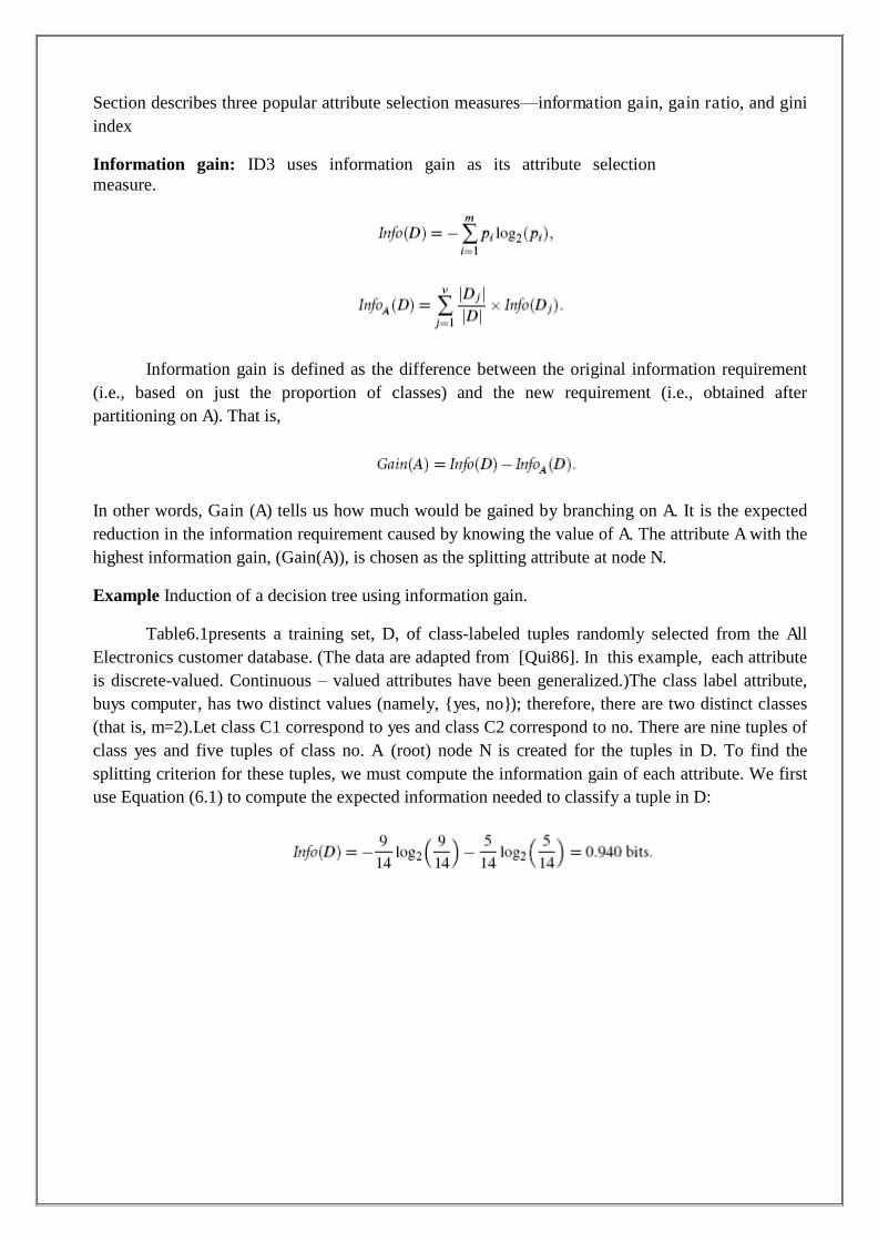
Section describes three popular attribute selection measures—information gain, gain ratio, and gini index

Information gain: ID3 uses information gain as its attribute selection measure.

Information gain is defined as the difference between the original information requirement (i.e., based on just the proportion of classes) and the new requirement (i.e., obtained after partitioning on A). That is,

In other words, Gain (A) tells us how much would be gained by branching on A. It is the expected reduction in the information requirement caused by knowing the value of A. The attribute A with the highest information gain, (Gain(A)), is chosen as the splitting attribute at node N.

Example Induction of a decision tree using information gain.

Table6.1presents a training set, D, of class-labeled tuples randomly selected from the All

Electronics customer database. (The data are adapted from [Qui86]. In this example, each attribute is discrete-valued. Continuous – valued attributes have been generalized.)The class label attribute, buys computer, has two distinct values (namely, { yes, no}); therefore, there are two distinct classes (that is, m=2).Let class C1 correspond to yes and class C2 correspond to no. There are nine tuples of class yes and five tuples of class no. A (root) node N is created for the tuples in D. To find the splitting criterion for these tuples, we must compute the information gain of each attribute. We fi rst use Equation (6.1) to compute the expected information needed to classify a tuple in D:

The expected information needed to classify a tuple in D if the tuples are partitioned according to Age is

Hence, the gain in information from such a partitioning would be

Similarly, we can compute Gain(income) = 0.029 bits, Gain(student) = 0.151 bits, and Gain(credit rating)=0.048bits.Because age has the highest information gain among the attributes, it is selected as the splitting attribute. Node N is labeled with age, and branches are grown for each of the attribute’s values. The tuples are then partitioned accordingly, as shown in Figure6.5. Notice that the tuples falling into the partition for age=middle aged all belong to the same class. Because they all belong to class “yes,” a leaf should therefore be created at the end of this branch and labeled with “yes.” The final decision tree returned by the algorithm is shown in Figure6.5.

4.9 BAYESIAN CLASSIFICATION

“What are Bayesian classifiers?” Bayesian classifiers are statistical classifiers. They can predict class membership probabilities, such as the probability that a given tuple belongs to a particular class.

Bayesian classification is based on Bayes’ theorem, a simple Bayesian classifier known as the naïve Bayesian classifier Bayesian classifiers have also exhibited high accuracy and speed when applied to large databases.

1) Bayes’ Theorem

.Let X be a data tuple. In Bayesian terms, X is considered ― evidence.‖ As usual, it is described by Measurements made on a set of n attributes. Let H be some hypothesis, such as that the data tuple X belongs to a specified class C. For classification problems, we want to determine P (Hj X), the probability that the hypothesis H holds given the― evidence ‖ or observed data tuple X. In other words, we are looking for the probability that tuple X belongs to class C, given that we know the attribute description of X.

“How are these probabilities estimated?” P(H),P(Xj H), and P(X) may be estimated from

the given data, as we shall see below. Bayes’ theorem is useful in that it provides away of calculating the posterior probability, P(Hj X),from P(H),P(Xj H),and P(X). Bayes’ theorem is

2) Naïve Bayesian Classif ication

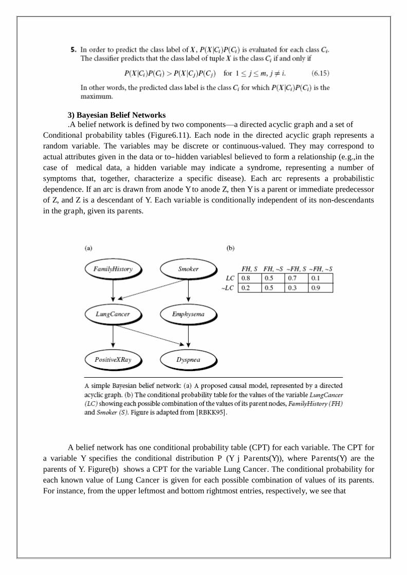
3) Bayesian Belief Networks .A belief network is defined by two components—a directed acyclic graph and a set of

Conditional probability tables (Figure6.11). Each node in the directed acyclic graph represents a random variable. The variables may be discrete or continuous-valued. They may correspond to actual attributes given in the data or to― hidden variables‖ believed to form a relationship (e.g.,in the case of medical data, a hidden variable may indicate a syndrome, representing a number of symptoms that, together, characterize a specific disease). Each arc represents a probabilistic dependence. If an arc is drawn from anode Y to anode Z, then Y is a parent or immediate predecessor of Z, and Z is a descendant of Y. Each variable is conditionally independent of its non-descendants in the graph, given its parents.

A belief network has one conditional probability table (CPT) for each variable. The CPT for a variable Y specifies the conditional distribution P (Y j Parents(Y)), where Parents(Y) are the parents of Y. Figure(b) shows a CPT for the variable Lung Cancer. The conditional probability for each known value of Lung Cancer is given for each possible combination of values of its parents. For instance, from the upper leftmost and bottom rightmost entries, respectively, we see that

Let X=(x1,:::, xn)be a data tuple described by the variables or attributes Y1,:::,Yn, respectively. Recall that each variable is conditionally independent to fi ts non descendants in the network graph, given its parents. This allows the network to provide a complete representation of the existing joint probability distribution with the

Following equation:

4.10 RULEBASED CLASSIFICATION Using IF-THEN Rules for Classif ication

Represent the knowledge in the form of IF-THEN rules

R: IF age=youth AND student =yes THEN buys_ computer=yes

O Rule antecedent/precondition vs. rule consequent Assessment of a rule: coverage and accuracy O ncovers=# of tuples covered by R oncorrect=# of tuples correctly classified by R o coverage(R)=ncovers/|D| /* D: training data set */ o accuracy(R) =ncorrect/ncovers If more than one rule is triggered, need conflict resolution O Size ordering: assign the highest priority to the triggering rules that has the

―toughest ‖requirement (i.e., with the most attribute test) O Class- based ordering: decreasing order of prevalence or misclassification co stper

class O Rule-based ordering(decision list):rules are organized into one long priority list,

according to some measure of rule quality or by experts Rule Extr action from a Decision Tree

Rules are easier to understand than large trees One rule is created for each path from the root to a leaf Each attribute-value pair along a path forms a co njunction: the leaf holds the class prediction Rules are mutually exclusive and exhaustive

Example: Rule extr action from our buys_ computer decision-tree

IF age=young AND student=no THEN buys_ computer=no

IF age=young AND student=yes IF age=mid-age

THEN buys _computer=yes THEN buys_ computer= yes

IF age=old AND credit _rating=excellent THEN buys _computer=yes IF age=young AND credit_ rating=fair THEN buys_ computer=no

Rule Extr action from the Training Data Sequential covering algorithm: Extracts rules directly from training data

Typical sequential covering algorithms: FOIL, AQ, CN2, RIPPER Rules are learned sequentially, each for a given class Ci will cover many tuples of Ci but none

(or few) of the tuples of other classes Steps:

O Rules are learned one at a time O Each time a rule is learned, the tuples covered by the rules are removed O The process repeats on the remaining tuples unless termination condition, e.g., when

No more training examples or when the quality of a rule returned is below a user- Specified threshold

Comp. w. decision-tree induction: learning a set of rules simultaneously 4.11 CLASSIFICATION B Y BACKPROPAGATION

Back propagation: A neural network learning algorithm Started by psychologists and neurobiologists to develop and test computational analogues of

neurons A neural network: A set of connected input / output units where each connection has a

Weight associated with it During the learning phase, the network learns by adjusting the weights so as to be able to predict the correct class label of the input tuples

Also referred to as connectionist learning due to the connections between units Neural Network as a Classif ier

Weakness O Long training time O Require a number of parameters typically best determined empirically, e.g., the

Network topology or`` structure."

O Poor interpretability: Difficult to interpret the symbolic meaning behind the learned

weights and of`` hidden units" in the network Strength

O High tolerance to noisy data O Ability to classify n trained patterns O Well-suited for continuous-valued inputs and outputs O Successful on a wide array of real-world data O Algorithms are inherently parallel O Techniques have recently been developed for the extraction of rules from trained

Neural networks A Neuron (=a perceptron)

Then- dimensional input vector x is mapped into variable y by means of the scalar product

and a non linear function mapping

A Multi-Layer Feed-Forward Neural Network

The inputs to the network correspond to the attributes measured for each training tuple

Inputs are fed simultaneously into the units making up the input layer They are then weighted and fed simultaneously to a hidden layer The number of hidden layers is arbitrary, although usually only one The weighted outputs of the last hidden layer are input to units making up the output layer,

which emits the network's prediction The network is feed-forward in that none of the weights cycles back to an input unit or to an

output unit of a previous layer From a statistical point of view, networks perform non linear regression: Given enough

hidden units and enough training samples, they can closely approximate any function

4.12 SVM—SUPPORT VECTOR MACHINES

A new classification method for both linear and nonlinear data It uses a nonlinear mapping to transform the original training data into a higher dimension With the new dimension, it searches for the linear optimal separating hyper plane (i.e.,

―decision boundary‖) With an appropriate non linear mapping to a sufficiently high dimension, data from two

classes can always be separated by a hyper plane SVM finds this hyper plane using support vectors (―essential ‖training tuples) and margins

(defined by the support vectors)

Features: training can be slow but accuracy is high owing to their ability to model

complex non linear decision boundaries (margin maximization) Used both for classification and prediction Applicat ions:

O handwritten digit recognition, object recognition, speaker identification, Bench marking time-series prediction tests

1) The Case When the Data Are Li nearly Separable An SVM approaches this problem by searching for the maximum marginal hyper plane.

Consider the below Figure, which shows two possible separating hyper planes and their associated margins. Before we get into the definition of margins, let’s take an intuitive look at this figure. Both hyper planes can correctly classif y all of the given data tuples. Intuitively, however, we expect the hyper plane with the larger margin to be more accurate at classifying future at a tuples than the hyper plane with the smaller margin. This is why (during the learning or training phase), the SVM searches for the hyper plane with the largest margin, that is, the maximum marginal hyper plane(MMH). The associated margin gives the largest separation between classes. Getting to an informal definition of margin, we can say that the shortest distance from a hyper plane to one side of its margin is equal to the shortest distance from the hyper plane to the other side of its margin, where the ― sides‖ of the margin are parallel to the hyper plane. When dealing with the MMH, this distance is, in fact, the shortest distance from the MMH to the closest training tuple of either class.

2) The Case When the Data Are Li nearly Inseparable

We learned about linear SVMs for classifying linearly separable data, but what if the data are not linearly separable no straight line can be found that would separate the classes. The linear SVMs we studied would not be able to find a feasible solution here. Now what?

The good news is that the approach described for linear SVMs can be extended to create

nonlinear SVMs for the classification of linearly inseparable data (also called nonlinearly separable data, or non linear data, for short).Such SVMs are capable of finding non linear decision boundaries (i.e., nonlinear hyper surfaces) in input space.

“So ,”you may ask,“ how can we extend the linear approach?” We obtain a non linear SVM by extending the approach for linear SVMs as follows. There are two main steps. In the fi rst step, we transform the original input data into a higher dimensional space using an on linear mapping. Several common non linear mappings can be used in this step, as we will describe further below. Once the data have been transformed into the new higher space, the second step searches for a linear separating hyper plane in the new space. We again end up with a quadratic optimization problem that can be solved using the linear SVM formulation. The maximal marginal hyper plane found in the new space corresponds to a non linear separating hyper surface in the original space.

4.13 ASSOCIATIVE CLASSIFICATION

Associative classification O Association rules are generated and analyzed for use in classification O Search for strong associations between frequent patterns (conjunction so f attribute-

value pairs) and class labels o Classification: Based on evaluating a set of rules in the form of

P1^p2 …^ pl―Aclass=C‖ (conf, sup) Why effective? O It explores highly confident associations among multiple attributes and may overcome

some constraints introduced by decision-tree induction, which considers only one attribute at a time

In many studies, associative classification has been found to be more accurate than some traditional classification methods, such as C4.

Typical Associative Classif ication Methods CBA (Classification By Association: Liu, Hsu& Ma, KDD’98)

O Mine association possible rules in the form of Cond-set (a set of attribute-value pairs) class label O Build classifier: Organize rules according to decreasing precedence based on

confidence and then support CMAR (Classification based on Multiple Association Rules: Li, Han, Pei, ICDM’01)

O Classification: Statistical analysis on multiple rules CPAR (Classification based on Predictive Association Rules: Yin &Han,SDM’03) O Generation of predictive rules (FOIL-like analysis) O High efficiency, accuracy similar to CMAR RCBT (Mining top-k covering rule groups for gene expression data, Cong et al.

SIGMOD’05) O Explore high-dimensional classification, using top-k rule groups O Achieve high classification accuracy and high run-time efficiency

4.14 LAZY LEARN ERS (ORLEARNIN G FROMYOUR NE IGHBORS)

The classification methods discussed so far in this chapter—decision tree induction, Bayesian classification, rule – based classification, classification by back propagation, support vector machines, and classification based on association rule mining—are all examples of eager learners . Eager learners, when given a set of training tuples, will construct a generalization (i.e., classification) model before receiving new(e.g., test) tuples to classify. We can think of the learned model as being ready and eager to classify previously unseen tuples.

1) k-Nearest- Neighbor Classifiers

The k- nearest – neighbor method was fi rst described in the early 1950s . The method is labor intensive when given large training sets, and did not gain popularity until the1960s when increased computing power became available. It has since been widely used in the area of pattern recognition.

Nearest-neighbor classifiers are based on learning by analogy, that is, by comparing a given

test tuple with training tuples that are similar to it. The training tuples are described by n attributes. Each tuple represents a point in an n- dimensional space. In this way, all of the training tuples are stored in an n- dimensional pattern space. When given an un known tuple, a k-nearest-neighbor classifier searches the pattern space for the k training tuples that are closest to the un known tuple. These k training tuples are the k―nearest neighbors ‖of the unknown tuple.

―Closeness ‖is defined in terms of a distance metric, such as Euclidean distance. The

Euclidean distance between two points or tuples, say, X1 =(x11,x12, : :: ,x1n) andX2 =(x21,x22, ::: ,x2n), is

2) Case-Based Reasoning Case-based reasoning (CBR) classifiers use a database of problem solutions to solve new

problems. Un like nearest –neighbor classifiers, which store training tuples as points in Euclidean space, CBR stores the tuples or― cases ‖for problem solving as complex symbolic descriptions. Business applications of CBR include problem resolution for customer service help desks, where cases describe product –related diagnostic problems. CBR has also been applied to areas such as engineering and law, where cases are either technical designs or legal rulings, respectively. Medical education is an other area for CBR, where patient case histories and treatments are used to help diagnose and treat new patients.

When given a new case to classify, a case –based reasoned will fi rst check if an identical training case exists .If one is found, then the accompanying solution to that case is returned. If no identical case is found, then the case-based reasoned will search for training cases having

Components that are similar to those of the new case. Conceptually, these training cases may be considered as neighbors of the new case. If cases are represented as graphs, this involves searching for sub graphs that are similar to sub graphs with in the new case. The case – based reasoned tries to combine the solutions of the neighboring training cases in order to propose a solution for the new case. If incompatibilities arise with the individual solutions, then backtracking to search for other solutions may be necessary. The case – based reasoned may employ background knowledge and problem- solving strategies in order to propose a feasible combined solution.

4.15 OTHERCLASSIFICATION METHODS

Genetic Algorithms Genetic Algorithm: based on an analogy to biological evolution

An initial population is created consisting of randomly generated rules O Each rule is represented by a string of bits O E.g., if A1 and ¬A2 then C2 can be encoded as 100 O If an attribute has k >2 values, k b its can be used Based on the notion of survival of the fit test, a new population is formed to consist of the

Fittest rules and their off springs The fitness of a rule is represented by its classification accuracy on a set of training examples Off springs are generated by crossover and mutation The process continues until a population P evolves when each rule in P satisfies a pre

specified threshold Slow but easily parallelizable

Rough Set Approach:

Rough sets are used to approximately or― roughly ‖define equivalent classes A rough set for a given class C is approximated by two sets: a lower approximation (certain

to be in C) and an upper approximation (cannot be described as not belonging to C) Finding the minimal sub sets (reducts) of attributes for feature reduction is NP- hard but a

discernibility ma tr ix (which stores the differences between attribute values for each pair of data tuples)is used to reduce the computation intensity

Figure: A rough set approximation of the set of tuples of the class C using lower and upper approximation sets of C. The rectangular regions represent equivalence classes

Fuzzy Set approaches

Fuzzy logic uses truth values between 0.0 and 1.0 to represent the degree of

membership (such as using fuzzy membership graph) Attribute values are converted to fuzzy values

O e.g., income is mapped into the discrete categories {low, medium, high} with fuzzy values calculated

For a given new sample, more than one fuzzy value may apply Each applicable rule contributes a vote for membership in the categories Typically, the truth values for each predicted category a re summed, and the sesum sare

combined

Prediction

(Numerical) prediction is similar to classification O construct a model O use model to predict continuous or ordered value for a given input Prediction is different from classification O Classification refers to predict categorical class label O Prediction models continuous-valued functions Major method for prediction: regression O model the relationship between one or more independent or predictor variables and a

Dependent or response variable Regression analysis O Linear and multiple regression O Non-linear regression O Other regression methods: generalized linear model, Poisson regression, log-linear

models, regression trees Li near Regression Linear regression: involves a response variable y and a single predictor variable x y=w0 +w1 x

where w0 (y-intercept) and w1 (slope) are regression coefficients Method of least squares: estimates the best-fitting straight line O Multiple linear regression: involves more than one predictor variable O Training data is of the form (X1,y1),(X2,y2),…,(X |D|, y|D|) O Ex. For2-D data, we may have: y=w0 +w1 x1+w2 x2

O Solvable by extension of least square method or using SAS, S-Plus O Many non linear functions can be transformed into the above

Non linear Regression Some nonlinear models can be modeled by a polynomial function A polynomial regression model can be transformed into linear regression model. For example, y=w0 +w1 x+ w2x

2+w3 x3

convertible to linear with new variables: x2=x2,x3=x3 y=w0 +w1 x +w2x2+w3 x3 Other functions, such as power function, can also be transformed to linear model Some models are intractable nonlinear (e.g., sum of exponential terms)

O possible to obtain least square estimates through extensive calculation on more complex formulae.

UNIT V CLUSTERING AN D APPLICATIONS AN D TRENDS IN DATA MINING Cluster Analysis – Types of Data – Categorization of Major Clustering Methods – K-means–

Partitioning Methods – Hierarchical Methods – Density-Based Methods –Grid Based Methods – Model-Based Clustering Methods – Clustering High Dimensional Data – Constraint – Based Cluster Analysis – Outlier Analysis – Data Mining Applications processors.

n1

n 1f 2f nf

5.1 TYPE OFDATA I N CLUSTERIN GANALYSIS

Data structure Data matr ix (two modes) object by variable Structure

x ... x ... x 11 ... ...

1f ...

...

1p...x ... x ... x i1 ...

... if ...

...

ip...

x ... x nf

... x

np

Dis similarity matrix (one mode) object–by-object structure

0 d(2,1) d(3,1)

0 d(3,2) 0 : : : d(n,1) d(n,2) ... ... 0

We describe how object dis similarity can be computed for object by Interval-scaled

variables,

Binary variables, Nominal, ordinal, and ratio variables, Variables of mixed types

Interval-Scaled variables (continuous measurement of a roughly linear scale) Standardize

data

Calculate the mean absolute deviation:

s1(|x m||x

m|...|x m|)

f n 1f f 2f f nf f

Where

mf

1(x x ...x).

Calculate the standardized measurement (z-score)

zi f x m if f

s

q q

Using mean absolute deviation is more robust than using standard deviation

Similarity and Dissimilarity Between Objects Distances are normally used to measure the similarity or dissimilarity between two data

objects Some popular ones include: Minkowski distance:

Where i =(xi1,xi2,…, xip)and j = (xj1,xj2,…, xjp) are two p-dimensional data objects, and q is a

positive integer

If q =1, d is Manhattan distance

d(i,j)|x x ||x x |...|x x | i1 j1 i2 j2 ip jp

d(i,j)q (|x xi1 j1|

|x xi2 j 2

| ...|x ip

xjp

|q) If q =2, d is Euclidean distance:

d(i,j) (|x x |2|x x |2...|x x |2) i1 j1 i2 j2 ip jp

Properties

d(i,j) 0 d(i,i) =0 d(i,j) =d(j,i) d(i,j)d(i,k)+d(k,j) Also, one can use weighted distance, parametric Pearson product moment correlation, or

other dissimilarity measures

Binary Var iables

A contingency table for binary data

Distance measure for symmetric binary variables:

M f

d(i,j) bc abcd

Distance measure for asymmetric binary variables:

d(i,j) bc abc

Jaccard coefficient (similarity measure for asymmetric binary variables):

Categorical variables

simJaccard

(i, j) a abc

A generalization of the binary variable in that it can take more than 2 states, e.g., red,

yellow, blue, green

Method1: Simple matching m: # of matches, p: total# of variables

d(i,j)pm

p Method2: use a large number of binary variables

creating a new binary variable for each of the M nominal states

Ordinal Variables An ordinal variable can be discrete or continuous Order is important, e.g., rank Can be treated like interval-scaled replace xif by the ir rank map the range of each variable onto [0, 1] by replacing i-th object in the f-th variable

by z rif1

if 1

compute the dis similarity using methods for interval-scaled variables

Ratio-scaled variable:

A positive measurement on a non linear scale, approximately at exponential scale, such as AeB tor

Ae-Bt

Methods:

treat them like interval-scaled variables—not a good choice! (why?—the scale

can be distorted)

apply logarithmic transformation yif=log(xif) treat them as continuous ordinal data treat their rank as interval-scaled

Var iables ofMixed Types

A database may contain all the six types of variables symmetric binary, asymmetric binary,

nominal, ordinal, interval and ratio

One may use a weighted formula to combine their effects p (f)d(f)

d(i, j) f1 ij ij p (f) Vector Objects f1 ij

Vector objects: key words in documents, gene features in micro-arrays, etc. Broad applications: information retrieval, biologic taxonomy, etc.

Cosine measure

A variant: Tani moto coefficient

5.2 CLUSTER ANALYSIS Cluster is a group of objects that belong to the same class. In other words the similar object are grouped in one cluster and dis similar are grouped in other cluster. Points to Remember

A cluster of data objects can be treated as a one group. While doing the cluster analysis, these to f data into groups based on data similarity and then

assign the label to the groups. The main advantage of Clustering over classification.

Applications of Cluster Analysis

Market research, pattern recognition, data analysis, and image processing. Characterize their customer groups based on purchasing patterns. In field of biology it can be used to derive plant and animal taxonomies, categorize genes

with similar functionality and gain insight into structures inherent in populations.

Clustering also helps in identification of areas of similar land use in an earth observation

database. It also helps in the identification of groups of houses in according house type, value, and geographic location.

Clustering also helps in classifying documents on the web for information discovery. Clustering is also used in outlier detection applications such as detection of credit card fraud. As a data mining function Cluster Analysis serve as a tool to gain insight into the distribution

of data to observe characteristics of each cluster. Requir ements of Clustering in Data Mining Here are the typical requirements of clustering in data mining:

Scalability – We need highly scalable clustering algorithms to deal with large databases. Abili ty to deal with different kind of attri butes- Algorithms should be capable to be

applied on any kind of data such as interval based (numerical) data, categorical, binary data. Discovery of clusters with attri bute shape- The clustering algorithm should be capable of

detect cluster of arbitrary shape. The should not be bounded to only distance measures that tend to find spherical cluster of small size.

High dimensionality- The clustering algorithm should not only be able to handle low- dimensional data but also the high dimensional space.

Abili ty to deal with noisy data- Databases contain noisy, missing or erroneous data. Some algorithms are sensitive to such data and may lead to poor quality clusters.

Interp retabili ty-The clustering results should be interpretable, comprehensible and usable. Clustering Methods

The clustering methods can be classified into following categories:

5.2.1 K means 5.2.2 Partitioning Method 5.2.3 Hierarchical Method 5.2.4 Density-based Method 5.2.5 Grid-Based Method 5.2.6 Model-Based Method 5.2.7 Constraint-based Method

5.2.1K-means

Given k, the k-means algorithm is implemented in four steps: 1. Partition objects into k non empty subsets 2. Compute seed points as the centroids of the clusters of the current partition (the

centroid is the center, i.e., mean point, of the cluster) 3. Assign each object to the cluster with the nearest seed point 4. Go back to Step 2, stop when no more new assignment

5.2.2Parti tioning Method Suppose we are given a database of n objects, the partitioning method construct k partition of data. Each partition will represent a cluster and k≤n. It means that it will classify the data into k groups, which satisfy the following requirements:

Each group contain at least one object. Each object must belong to exactly one group.

Typical methods:

K-means, k-medoids, CLARANS 5.2.3Hierarchical Methods This method creates the hierarchical decomposition of the given set of data objects.:

Agglomerative Approach Divisive Approach

Agglomerative Approach This approach is also known as bottom-up approach. In this we start with each object forming a Separate group. It keeps on merging the objects or groups that are close to one another. It keep on doing so until all of the groups are merged into one or until the termination condition holds.

Divisive Approach This approach is also known as top-down approach. In this we start with all of the objects in the Same cluster. In the continuous iteration, a cluster is split up into smaller clusters. It is down until each object in one cluster or the termination condition holds.

Disadvantage This method is rigid i.e. once merge or split is done, It can never be undone. Approaches to improve quality of Hi erarchical clustering Here is the two approaches that are used to improve quality of hierarchical clustering:

Perform careful analysis of object linkages at each hierarchical partitioning. Integrate hierarchical agglomeration by fi rst using a hierarchical agglomerative algorithm to

group objects into micro clusters, and then performing macro clustering on the micro clusters.

Typical methods: Diana, Agnes, BIRCH, ROCK, CAMELEON BIRCH (1996): uses CF-tree and incrementally adjusts the quality of sub-clusters

Incrementally construct a CF(Clustering Feature) tree, a hierarchical data structure for multiphase clustering Phase1: scan DB to build an initial in-memory CF tree (a multi-level compression of

the data that tries to preserve the inherent clustering structure of the data) Phase2: use an arbitrary clustering algorithm to cluster the leaf nodes of the CF-tree

Clustering Feature: CF = (N, LS, SS)

ROCK (1999): clustering categorical data by neighbor and link analysis Robust Clustering using links Major ideas

O Use links to measure similarity/proximity O Not distance-based O Computational complexity: Algorithm: sampling-based clustering O Draw random sample O Cluster with links O Label data in disk

O CHAMELEON (1999): hierarchical clustering using dynamic modeling Measures the similarity based on a dynamic model O Two clusters are merged only if the interconnectivity and closeness (proximity)

between two clusters are high relative to the internal inter connectivity of the clusters and closeness of items within the clusters

O Cure ignores information about inter connectivity of the objects, Rock ignores information about the closeness of two clusters A two-phase algorithm

O Use a graph partitioning algorithm: cluster objects into a large number of relatively small sub-clusters

O Use an agglomerative hierarchical clustering algorithm: find the genuine clusters by

repeatedly combining these sub-clusters

5.2.4Density-based Method Clustering based on density (local cluster criter ion), such as density-connected points Major features:

O Discover clusters of arbitrary shape O Handle noise O One scan O Need density parameters as termination condition Two parameters: O Eps : Maximum radius of the neighbor hood O Min Pts: Minimum number of points in an Eps- neighbor hood of that point Typical methods: DBSACN, OPTICS, Den Clue DBSCAN: Density Based Spatial Clustering of Applications with Noise Relies on a density-based notion of cluster: A cluster is defined as a maximal set of density-

connected points Discovers clusters of arbitrary shape in spatial databases with noise DBSCAN: The Algorithm Arbitrary select a point p Retrieve all points density-reachable from p w.r.t .Eps and Min Pts. If p is a core point, a cluster is formed. If p is a border point, no points are density-reachable from p and DB SCAN visits the next

point of the database. Continue the process until all of the points have been processed.

O OPTICS: Ordering Points To Identify the Clustering Structure O Produces a special order of the database with its density- based clustering structure O This cluster-ordering contains info equiv to the density-based clustering’s

Corresponding to a broad range of parameter settings O Good for both automatic and interactive cluster analysis, including finding intrinsic

clustering structure O Can be represented graphically or using visualization techniques DENCLUE: DEN sity -based CLU st Ering Major features O Solid mathematical foundation O Good for data sets with large amounts of noise O Allows a compact mathematical description of arbitrarily shaped clusters in high-

Dimensional datasets O Significant faster than existing algorithm (e.g., DBSCAN) O But needs a large number of parameters

5.2.5Grid-based Method

O Using mult i-resolution grid data structure Advantage The major advantage of this method is fast processing time. It is dependent only on the number of cells in each dimension in the quantized space. Typical methods: STING, Wave Cluster, CLIQUE STING: a Statistical INformation Grid approach The spatial area is divided into rectangular cells There are several levels of cells corresponding to different levels of resolution

O Each cell at a high level is partitioned into a number of smaller cells in the next lower

level O Statistical info of each cell is calculated and stored before hand and is used to answer

queries O Parameters of higher level cells can be easily calculated from parameters of lower

level cell count, mean, s, min, max type of distribution—normal, uniform, etc.

O Use a top-down approach to answer spatial data queries O Start from a pre-selected layer—typically with a small number of cells O For each cell in the current level compute the confidence interval Wave Cluster: Clustering by Wavelet Analysis A multi-resolution clustering approach which applies wavelet transform to the feature space How to apply wavelet transform to find clusters O Summarizes the data by imposing a multidimensional grid structure onto data space O These multidimensional spatial data objects are represented in a n-dimensional

Feature space O Apply wavelet transform on feature space to find the dense regions in the feature

space O Apply wavelet transform multiple times which result in clusters at different scales

from fine to coarse Wavelet transform: A signal processing technique that decomposes a signal into different frequency sub-band (can be applied to n-dimensional signals) Data are transformed to preserve relative distance between objects at dif ferent levels of resolution Allows natural clusters to become more distinguishable

5.2.6Model-based methods

O Attempt to optimize the fit between the given data and some mathematical model O Based on the assumption: Data are generated by a mixture of underlying

probability distri bution In this method a model is hypothesize for each cluster and find the best fit of data to the

given model.

This method also serve away of automatically determining number of clusters based on

standard statistics, taking outlier or noise into account. It therefore yields robust clustering methods. Typical methods: EM, SOM, COBWEB

EM — A popular iterative refinement algorithm An extension to k-means O Assign each object to a cluster according to a weight (prob. distribution) o New means are computed based on weighted measures General idea O Starts with an initial estimate of the parameter vector O Iteratively rescores the patterns against the mixture density produced by the

parameter vector o The rescored patterns are used to update the parameter updates o Patterns belonging to the same cluster, if they are placed by their scores in a

particular component Algorithm converges fast but may not be in global optima COBWEB(Fisher’87)

O A popular a simple method of incremental conceptual learning O Creates a hierarchical clustering in the form of a classification tree o Each node refers to a concept and contains a probabilistic description of that concept

O SOM (Soft-Organizing feature Map) O Competitive learning Involves a hierarchical architecture of several units (neurons) Neurons compete in a― winner- takes- all‖ fashion for the object currently

Being presented SOMs, also called topological ordered maps, or Kohonen Self-Organizing FeatureMap (KSOMs) It maps all the points in a high- dimensional source space into a 2 to 3- d target space, s.t .,the distance and proximity relationship (i.e., topology) are preserved as much as possible Similarty ok-means: cluster centers tend to lie in a low- dimensional fold in the feature space

Clustering is performed by having several units competing for the current object

O The unit whose weight vector is closest to the current object wins O The winner and its neighbors learn by having their weights adjusted SOMs are believed to resemble processing that can occur in the brain Useful for visualizing high-dimensional data in 2-or3-D space

5.2.7Constraint-based Method Clustering by considering user- specified or application-specific constraints Typical methods: COD(obstacles), constrained clustering Need user feedback: Users know their applications the best Less parameters but more user-desired constraints, e.g., an ATM allocation problem:

Obstacle & desired clusters Clustering in applications: desirable to have user-guided (i.e., constrained)cluster analysis Different constraints in cluster analysis:

O Constraints on individual objects (do selection first) Cluster on houses worth over$300K O Constraints on distance or similarity functions Weighted functions, obstacles (e.g., rivers, lakes) O Constraints on the selection of clustering parameters # of clusters, Min Pts, etc. O User-specified constraints Contain at least 500 valued customers and 5000 ordinary ones O Semi- supervised: giving small training sets as ―constraints‖ or hints Example: Locating k delivery centers, each serving atleast m valued customers and n

ordinary ones Proposed approach O Find an initial―solution ‖by partitioning the data set into k groups and satisfying

user- constraints o Iteratively refine the solution by micro-clustering relocation (e.g., moving δ μ-

clusters from cluster Ci to Cj) and― deadlock ‖handling (break the micro clusters when necessary)

o Efficiency is improved by micro-clustering How to handle more complicated constraints? O E.g., having approximately same number of valued customers in each cluster?!—

Can you solve it? 5.3 OUTLIER ANALYSIS

The set of objects are considerably dissimilar from the remainder of the data

O Example: Sports: Michael Jordon, Wayne Gretzky,... Problem: Define and find outliers in large data sets

Applications: Credit card fraud detection Telecom fraud detection Customer segmentation

Medical analysis

Statistical Distri bution- based outlier detection- Identify the outlier with respect to the model

using discordancy test

How discordancy test work

Data is assumed to be part of a working hypothesis (working hypothesis)-H

Each data object t in the data set is compared to the working hypothesis and is either accepted in

the working hypothesis or rejected as discordant into an alternative hypothesis (outliers)-H

Working Hypothesis: H:oi F,wherei1,2,...,n.

Discordancy Test: isoi inFwithinstandarddeviation15

Alternative Hypothesis:

-Inherent Distribution:H:oi G,wherei1,2,...,n.

Mixture Distribution:

-Slippage Distibution:

H:oi (1)FG,wherei1,2,...,n.

H:oi (1)FF,wherei1,2,...,n.

Distance-Based outlier detection

Imposed by statistical methods

We need multi-dimensional analysis without knowing data distribution

Algorithms for mining distance-based outliers Index-based algorithm Indexing Structures such as R-tree(R+-tree), K-D (K-D-B) tree are built for the multi-

dimensional database

The index is used to search for neighbors of each object O within radius D around that

object.

Once K (K=N(1-p)) neighbors of object O are found, O is not an outlier.

Worst-case computation complexity is O (K* n2), K is the dimensionality and n is the

number of objects in the data set.

Pros: scale well with K Cons: the index construction process may cost much time Nested-loop algorithm Divides the buffer space into two halves (fi rst and second arrays) Break data into blocks and then feed two blocks into the arrays.

Directly computes the distance between each pair of objects, inside the array or between

arrays

Decide the outlier. Here comes an example:… Same computational complexity as the index-based algorithm Pros: Avoid index structure construction Try to minimize the I/Os

Cell based algorithm Divide the data set into cells with length K is the dimensionality, D is the distance Define Layer-1 neighbors– all the intermediate neighbor cells. The maximum distance

between a cell and its neighbor cells is D

Define Layer- 2 neighbors –the cells within 3 cell of a certain cell. The minimum

distance between a cell and the cells outside ofLayer-2 neighbors is D

Criteria Search a cell internally. If there are M objects inside, all the objects in this

cell are not outlier

Search its layer- 1 neighbors. If there are M objects inside a cell and its layer-

1neighbors, all the objects in this cell are not outlier Search its layer- 2 neighbors. If there are less than M objects inside a cell, its

layer-1 neighbor cells, and its layer- 2 neighbor cells, all the objects in this

cell are outlier

Otherwise, the objects in this cell could be outlier, and then need to calculate

the distance between the objects in this cell and the objects in the cells in the

layer -2 neighbor cells to see whether the total points with in D distance is

more than M or not.

Density-Based Local Outlier Detection Distance-based outlier detection is based on global distance distribution It encounters difficulties to identif y outliers if data is not uniformly distributed Ex.C1 contains400 loosely distributed points, C2 has 100 tightly condensed points, 2 outlier

points o1, o2

Some outliers can be defined as global outliers, some can be defined as local outliers to a

given cluster

O2 would not normally be considered an outlier with regular distance-based outlier detection,

since it looks at the global picture

Each data object is assigned a local outlier factor (LOF) Objects which are closer to dense clusters receive a higher LOF LOF varies according to the parameter Min Pts

Deviation-Based Outlier detection Identifies outliers by examining the main characteristics of objects in a group Objects that ―deviate ‖from this description are considered outliers

Sequential exception technique simulates the way in which humans can distinguish un usual objects from among a series of

supposedly like objects

Dissimilarities are assed between subsets in the sequence the techniques introduce the

following key terms

Exception set, dis similarity function, cardinality function, smoothing factor

OLAP data cube technique Deviation detection process is overlapped with cube computation Recomputed measures indicating data exceptions are needed A cell value is considered an exception if it is significantly different from the expected value,

based on a statistical model

Use visual cues such as back ground color to reflect the degree of exception

5.4 DATA MINING APPLICATIONS

Here is the list of areas where data mining is widely used: Financial Data Analysis Retail Industry Telecommunication Industry Biological Data Analysis Other Scientific Applications Intrusion Detection

Financial Data Analysis

The financial data in banking and financial industry is generally reliable and of high quality which

facilitates the systematic data analysis and data mining. Here are the few typical cases:

Design and construction of data warehouses for multidimensional data analysis and data

mining.

Loan payment prediction and customer credit policy analysis. Classification and clustering of customers for targeted marketing. Detection of money laundering and other financial crimes.

Retail Industry

Data Mining has its great application in Retail Industry because it collects large amount data from

on sales, customer purchasing history, goods transportation, consumption and services. It is natural

that the quantity of data collected will continue to expand rapidly because of increasing ease,

availability and popularity of web.

The Data Mining in Retail Industry helps in identifying customer buying patterns and trends. That

leads to improved quality of customer service and good customer retention and satisfaction. Here is

the list of examples of data mining in retail industry:

Design and Construction of data warehouses based on benefits of data mining. Multidimensional analysis of sales, customers, products, time and region. Analysis of effectiveness of sales campaigns.

Customer Retention.

Product recommendation and cross-referencing of items.

Telecommunication Industry

Today the Telecommunication industry is one of the most emerging industries providing various

services such as fax, pager, cellular phone, Internet messenger, images, e-mail, web data

transmission etc. Due to the development to new computer and communication technologies, the

telecommunication industry is rapidly expanding. This is the reason why data mining is become

very important to help and understand the business.

Data Mining in Telecommunication industry helps in identifying the telecommunication patterns,

catch fraudulent activities, make better use of resource, and improve quality of service. Here is the

list examples for which data mining improve telecommunication services:

Multidimensional Analysis of Telecommunication data. Fraudulent pattern analysis. Identification of unusual patterns. Multidimensional association and sequential patterns analysis. Mobile Telecommunication services. Use of visualization tools in telecommunication data analysis.

Biological Data Analysis

Now a days we see that there is vast growth in field of biology such as genomics, proteomics,

functional Genomics and biomedical research. Biological data mining is very important part of Bio

informatics. Following are the aspects in which Data mining contribute for biological data analysis:

Semantic integration of heterogeneous , distributed genomic and proteomic databases. Alignment, indexing, similarity search and comparative analysis multiple nucleotide

sequences.

Discovery of structural patterns and analysis of genetic networks and protein pathways. Association and path analysis. Visualization tools in genetic data analysis.

Other Scientific Applications

The applications discussed above tend to handle relatively small and homogeneous data sets for

which the statistical techniques are appropriate. Huge amount of data have been collected from

scientific domains such as geo sciences, astronomy etc. There is large amount of data sets being

generated because of the fast numerical simulations in various fields such as climate, and ecosystem

modeling, chemical engineering, fluid. Following are the applications of data mining in field of

Scientific Applications:

Data Warehouses and data preprocessing. Graph-based mining. Visualization and domain specific knowledge. Intrusion Detection

Intrusion refers to any kind of action that threatens integrity, confidentiality, or availability of

network resources. In this world of connectivity security has become the major issue. With

increased usage of internet and availability of tools and tricks for intruding and attacking network

prompted intrusion detection to become a critical component to f network administration. Here is the

list of areas in which data mining technology may be applied for intrusion detection:

Development of data mining algorithm for intrusion detection. Association and correlation analysis, aggregation to help select and build discriminating

attributes.

Analysis of Stream data. Distributed data mining. Visualization and query tools.

M.I.E.T. ENGINEERING COLLEGE/ DEPT. of CSE

M.I.E.T. /CSE / III /DATAWAREHOUSING & DATAMINING