DEPARTMENT OF ECONOMICS

Working Paper

Steindlian models of growth and stagnation

Peter Flaschel and Peter Skott

Working Paper 2004-11

Revised version, September 2004

UNIVERSITY OF MASSACHUSETTS AMHERST

Steindlian models of growth and stagnation∗

Peter FlaschelFaculty of EconomicsBielefeld UniversityPO Box 10 01 31

33501 Bielefeld, Germany

Peter SkottDepartment of Economics

Thompson HallUniversity of MassachusettsAmherst, MA 01003, USA

Revised version

September 22, 2004

Abstract

Following an analysis of the relation between a standard Steindlian model ofstagnation and Steindl’s own analysis, we modify the standard model by introducingendogenous changes in the markup and a reformulation of the investment function.These extensions, which address significant weaknesses of the standard model, findsupport in Steindl’s writing and leave intact some of Steindl’s key results. In a furtherextension, we add a labour market and analyse the stabilizing influence of a Marxianreserve-army mechanism. The implications of the extended model for the effects ofincreased oligopolization are largely in line with Steindl’s predictions.

JEL CLASSIFICATION SYSTEM FOR JOURNAL ARTICLES:E24, E31, E32.

KEYWORDS: Steindl, accumulation, stagnation, markup, monopolization, reservearmy of labour

∗Early versions of this paper have been presented at the Steindl conference, Vienna, September 2003,and at a seminar at CEPA, New York. We thank participants in these meetings and two anonymousreferees for helpful comments and suggestions.

1

2

1 Introduction

Steindl explained the depression in the interwar period by the inability of the economy“to adjust to low growth rates because its saving propensity is adapted to a high one”(Steindl 1979, p.1) The argument was laid out in Steindl (1952). In the process of capi-talist development, he argued, previously competitive industries become oligopolized. Thischange in competitive conditions puts upward pressure on the profit margin and makes theprofit margin less responsive to changes in demand conditions. An increase in the profitmargin may provide the trigger for reduced demand and a reduction in growth rates; theinsensitivity of the margin to lower demand and the emergence of unwanted excess capac-ity potentially turn the downturn into secular depression or stagnation. The economy, inhis terminology, becomes ‘mature’, where maturity is defined “as the state in which theeconomy and its profit function are adjusted to the high growth rates of earlier stages ofcapitalist development, while those high growth rates no longer obtain” (1979, p. 7).

The postwar economy was revitalized and experienced a golden age with near full employ-ment and high growth rates from the 1950s to around 1970. This golden age, in Steindl’sview, was explained by a combination of expansionary policy (large increases in the gov-ernment sector in all OECD countries), an acceleration of R&D stimulated by the coldwar, increased cooperation between western countries, and the potential for technologicalcatch-up in both Europe and Japan. The stimulus from these factors, he argued, was tem-porary, and other influences also contributed to a re-assertion of stagnationist tendencies inthe 1970s. Steindl singles out, in particular, an increasing trend of personal saving and “achanged attitude of governments towards full employment and growth” (1979, p. 12). Thislatter influence, which is seen as “the most striking feature of the new economic climate”(1979, p. 12), is explained in terms of a Kaleckian political cycle “as a reaction against thelong period of full employment and growth which has strengthened the economic positionof workers and the power of the trade unions, and has led to demands for workers’ partici-pation” (p. 12-13). Writing in 1979, Steindl therefore expected “low growth for some timeto come”.

It is beyond the scope of this paper to attempt an empirically based evaluation of Steindl’stheory.1 Our aim is more modest and almost entirely theoretical. Steindl’s contributionsto an understanding of capitalist growth and stagnation have been highly influential butre-reading his original studies, we have been struck by the fact that important aspects ofhis argument appear to have been left out of subsequent models. In this paper we try toclarify the connection between a ‘standard Steindlian model’ and Steindl’s own analysis.Secondly, and more importantly, we extend the standard model to include some of theaspects of his analysis that have been left out.

1We have reservations with respect to some of his claims. The existence of an increasing trend inmonopolization, for instance, is debatable (e.g. Semmler (1984), Auerbach (1988) and Auerbach and Skott(1988)).

3

Most Steindlian models focus on the product market and treat the markup as exogenous.We outline a standard model of this kind in section 2. Unlike Steindl’s (1952) own model,which is set up as mixed difference-differential equations and which has multiple steadygrowth solutions, the standard model is cast entirely in continuous time and has a uniquesteady growth solution. In some respects the standard model does a good job of capturingSteindl’s argument, and the switch to a continuous-time setting simplifies the analysisenormously. However, the standard model also has weaknesses, both on its own terms andfrom an exegetical perspective. One weakness is the use of an exogenous markup. Thisassumption clashes with Steindl’s verbal analysis of how “elastic profit margins” tend toeliminate undesired excess capacity in competitive industries and how the “growth of themonopolistic type of industry may lead to a fundamental change in the working of theeconomy: bringing about greater inelasticity of profit margins” (1952, p. ix). A secondweakness concerns the specification of the long-run investment function. The standardmodel differs from Steindl’s own specification in this respect and there are, we shall argue,problems with the standard model as well as with Steindl’s own analysis.

Section 3 presents a reformulation of the standard model which addresses the two weak-nesses. The reformulation, first, introduces Steindlian movements in the markup. Thus,we assume that the markup will be rising when actual capacity utilization exceeds desiredutilization. Other models exist, of course, in which the mark-up changes endogenously,but in these models the determination of the changes is rather different. Dutt (1984), forinstance, relates changes in the markup to the rate of growth of the economy while Sawyer(1995) allows the level of the markup to depend on the rate of utilization (as indeed didKalecki (1954)). Although still different, the specifications in Taylor (1985) and Lavoie(1995) which relate changes of the markup to the profit rate come closer to the Steindlianposition.

Our second extension of the standard model concerns the investment function. We respecifythis function to allow for a distinction between the short-run and the long-run sensitivityof the accumulation rate to changes in utilization. This distinction - central to modelsin a Harrodian tradition and discussed at some length in Skott (1989a) - is included inSteindl’s formal 1952 model as well as in Dutt’s (1995) more recent formalization of Steindl’stheory. Our specification of the function in this paper is much simpler than Steindl’s andmore general than Dutt’s. The main contribution of the extension, however, lies in thecombination of the new investment function with a Steindlian markup dynamics.

Both of the extensions in section 3 find support in Steindl’s writing, and they significantlyinfluence the properties of the system. If the new investment function is used in the standardmodel without markup dynamics, the steady growth path is likely to become unstable. Themarkup dynamics has a stabilizing influence and the combined model may, but need not,produce a stable steady-growth path. In the stable case, increasing oligopolization leadsto a decline in both the rate of growth and the utilization of capital but, paradoxically, to

4

a fall in the share of profits. Thus, the stable case leaves intact some but not all of keyresults of the standard model.

In section 4 we go beyond the analysis of the product market. Both financial and labourmarkets play important roles in Steindl’s verbal argument; financial markets because ofSteindl’s emphasis on internal finance and changes in household saving, and labour marketsbecause Steindl regarded prolonged full employment in the 1950’s and 1960s as a key factorbehind the subsequent stagnation. Financial extensions of the standard model have beenexplored by Dutt (1995) and in this paper we make no attempt to pursue this aspect ofSteindl’s analysis. Our emphasis, instead, is on the labour market.

A labour market has been introduced into Steindlian models by Dutt (1992), among others.Our specification, however, differs substantially from his. Following Steindl’s (1979) argu-ment we let the rate of employment affect firms’ investment decisions and show that theimplications of this extended model for the effects of increased oligopolization are largely inline with Steindl’s predictions, at least for a range of parameter values. Dutt, by contrast,considers the influence of the rate of employment on wage inflation. He assumes that firms’pricing decisions fail to neutralize these nominal changes in the wage. Thus, the labourmarket enters his model because of its effects on (the rate of change of) the markup. Thismechanism is akin to the one in Goodwin (1967) and other models in which a real-wagePhillips curve generates a rising real wage and a falling markup when employment is high.It should be noted that if one assumes that the employment and utilization rates movetogether and can be represented by the same variable, a real-wage Phillips curve impliesan inverse relation between utilization and the change in the markup - the opposite of theSteindlian assumption.2

The paper closes, in section 5, with some conclusions and remarks on future work.

2 Steindl and the standard model

2.1 A standard model in continuous time

We consider a closed economy without public sector. Output is produced using two in-puts, labour and capital, and the production function has fixed coefficients. It would bestraightforward to include Harrod-neutral technical change but we leave out this elementto simplify the exposition. It is assumed that firms retain a proportion sf of profits anddistribute the rest to households in the form of interest payments and dividends, and that

2Since it simplifies the analysis, the assumption of a (near-)perfect correlation between the rates ofemployment and capital utilization is common in the literature. The assumption may be legitimate in theshort run but the ratio of the capital stock to the labour force is neither constant nor exogenously given,and the assumption can be highly misleading in the long run.

5

there is a uniform saving rate s out of distributed incomes, including wages.3 Investmentis positively related to the rate of utilization of the capital stock and may also dependpositively on retained earnings. Algebraically, the (net) investment and saving functionsare given by

I

K= a+m(u− 1) + bsfπ

u

k(1)

S

K= sfπ

u

k+ s(1− π + (1− sf)π)

u

k= s(π)

u

k(2)

where I, S and K denote investment, saving and the capital stock, k is the capital-outputratio at the desired utilization rate (normalized to one), u the actual utilization rate andπ the share of profits in income (u/k and πu/k thus define the actual output-capital ratioand the profit rate). The average saving rate out of income is s(π) = sf(1− s)π + s. Allvariables are contemporaneous, and the parameters m, b, sf and s are positive.

The equilibrium condition for the product market can be written

a+m(u− 1) + bsfkπu =

u

k[sf(1− s)π + s] =

s(π)

ku (3)

This equation determines the rate of capacity utilization u as a function of the profit shareπ. The profit share itself is determined by an exogenously given markup on unit labourcost (π = (β − 1)/β where β is the markup).Solving equation (3) for u we get

u =k(a−m)

s+ sf(1− s− b)π −mk(4)

Using standard assumptions for the adjustment process, the stability of this short-runequilibrium requires that investment be less sensitive than investment to variations inoutput; that is, mk + bsfπ < s(π). When this ‘Keynesian stability condition’ is imposed,the constant a in the accumulation function function must satisfy the restriction a > m inorder for the model to produce a positive rate of utilization.

Equations (1)-(4) give rise to Marglin-Bhaduri (1990) possibilities of exhilarationist orstagnationist outcomes. Assuming that the Keynesian stability condition holds, an increasein the profit share will lead to a decline in utilization if the ‘Robinsonian stability condition’0 < [sf(1− s− b)] is satisfied; a reversal of this Robinsonian condition implies that u will

3A uniform saving rate out of distributed incomes is in line with Steindl’s specification (1952, p. 214,equation (40 vii)). In the presence of retained earnings, the aggregate saving rate depends positively onthe profit share. Thus, the introduction of differential saving rates sp and sw for household saving out ofwage income and distributed profits would leave the structure of the model substantively unchanged.

6

rise with π and thus will fall with increases in the real wage.4 The effects on growth areambiguous. Differentiating g = s(π)

ku(π) with respect to π, we get

∂g

∂π=

u

k

∙s(π)

−sf(1− s− b)

s+ sf(1− s− b)π −mk+ sf(1− s)

¸=

usfk

sb− (1− s)mk

s+ sf(1− s− b)π −mk

Hence, if both the Keynesian short-run stability condition and the Robinsonian stabilitycondition are met, an increase in the profit share will have a negative impact on growth if

sb < (1− s)mk.

This ambiguous conclusion mirrors the results in Steindl (1952). Thus, Steindl (1952, p.224) finds that a rise in the markup depresses growth if the direct effect of the profit shareon investment is small relative to the effect of utilization on investment, a condition whichis similar to the condition above.

Overall, a linear model with a constant term in the investment function and parameterrestrictions that ensure Keynesian and Robinsonian stability might appear to capture thespirit of Steindl’s argument. It is not surprising therefore that following early contributionsby Rowthorn (1981) and Dutt (1984) and subsequent work by, among others, Taylor (1985),Sawyer (1985) and Marglin and Bhaduri (1990), a model along these lines has become thestandard formalization of the Kalecki-Steindl theory.

The rest of this section examines the relation between the standard model and Steindl’s(1952) formalization in greater detail. Readers with no interest in this relation may skipdirectly to section 3.

2.2 The 1952 argument

Steindl’s formal model of an economy with variable utilization (1952, pp. 211-228) is castin terms of mixed difference-differential equations. The key investment equation (equation(39), p. 213) can be written

It+θ = γCt + q (Ct − g0Kt) +m(kYt − u0Kt) (5)

where θ is a discrete investment lag, k is the ratio of the stock of capital to productivecapacity and u0 the desired utilization rate; the impact of financing conditions are capturedby the retained earnings C and the stock of "entrepreneurs’ capital" C; g0 is the inverse

4Although logically possible and used in some models, the condition for Robinsonian instability seemsimplausible: empirical evidence suggests that the impact effect of changes in real wages falls mainly onconsumption, rather than investment.

7

of the desired gearing ratio; a dot over a variable is used to denote a rate of change (i.e.x = dx

dt) and the parameters γ, q andm are all positive.5 Using assumptions similar those of

the standard model concerning the determination of retained earnings and personal saving,Steindl derives a dynamic equation for the evolution of the capital stock,

..

Kt+θ − L..

Kt +MKt +NKt = 0 (6)

where the composite parameters L,M and N can be expressed in terms of the underlyingparameters from the functions describing investment and saving.

To solve equation (6), Steindl assumes that the equation represents "a long-run model ofmoving averages" (p. 227) and that long-run movements may plausibly be described byexponential trends determined by the real roots of (6). Thus, implicitly it is assumed thatthe initial conditions (i.e. the trajectory of the system over a time interval correspondingto the discrete lag θ) can be written

K(t) =X

ci exp ρit (7)

where the ci ’s are constants and the ρi ’s represent the real roots of the characteristicequation

ρ2 exp(θρ)− Lρ2 +Mρ+N = 0 (8)

Given these initial conditions, the full solution to equation (6) also takes the form (7).

The next step is to find the real roots of (8). It turns out that in order to get anypositive roots, additional restrictions on the parameter values have to be introduced. Theserestrictions reverse the Keynesian stability condition in the standard model. Thus usingthe notation of the standard model, Steindl’s necessary condition for positive roots (p. 219)is that

mk + bπsfs(π)

> 1

which is the condition for Keynesian instability in the standard model.

Assuming that positive roots exist, the equation will have three real roots and the move-ments of the capital stock can be described by

K(t) = c1eρ1t + c2e

ρ2t + c3eρ3t

where ρ1 < 0 < ρ2 < ρ3. Asymptotically, the largest of the three roots dominates the move-ments in K and, Steindl concludes, the capital stock must therefore grow asymptoticallyat the high rate ρ3.6

5Steindl (1952, p. 213) uses Z rather than the standard notation K to denote the capital stock.6Steindl (incorrectly) suggests that it is the root which is largest in absolute value that will dominate.

No harm is done, however, since the large root ρ3 happens to be the largest in absolute value. The analysis

8

The comparative statics of the steady growth path associated with ρ3 can now be examined.From a Steindlian perspective, the effects of increasing oligopolization are particularlyinteresting. Increasing ologopolization is associated with an upward shift of the profitfunction (that is, the markup).7 This shift, Steindl finds, produces a decline in the rateof growth, as long as the expansionary financial effects on investment (represented by theparameters γ and q in equation (5)) are weak relative to the effect of utilization (representedby mk in equation (5)). This condition seems plausible, and the results are strengthenedif the rise in the degree of monopoly also leads to increased fears of excess capacity in theindustry and a corresponding increase in the desired utilization rate u0.8 Thus, the modelappears to support Steindl’s central conclusion:

On the basis of the present model it is thus possible to demonstrate that thedevelopment of monopoly may bring about a decline in the rate of growth ofcapital. I believe that this is, in fact, the main explanation of the decline in therate of growth which has been going on in the United States from the end ofthe last century. (p. 225)

Unfortunately, the empirical application of the model raises difficulties, and Steindl isrefreshingly forthright and clear about these difficulties He points out that "if plausiblevalues are given to the structural coefficients ... then it appears that the limiting rate ofgrowth thus obtained is very big" (p. 226). This problem is serious since it implies thatit "is difficult to explain, on the basis of my model, moderate rates of growth, such as hasbeen observed in the history of capitalism" and "either the model requires modifications inimportant respects in order to be realistic, or else, it follows that an exponential trend inthe strict mathematical sense is not a proper description of long-run growth" (p. 226).

(p. 220) is slightly flawed also by a failure to realize that the capital stock will be declining from some pointonwards (and reach zero in finite time) if the coefficient c3 associated with the dominant root is negative.Meaningful non-negative solutions for the long-run capital stock require that the initial conditions are suchthat c3 > 0 (or, alternatively, such that either c2 > c3 = 0 or c1 > c2 = c3 = 0); implicitly, Steindl’sanalysis presumes that c3 > 0.Note finally that although the stability analysis is conditional on very restrictive assumptions concerning

the initial conditions, it is not quite correct, as suggested by Dutt (1995, p. 17), that Steindl "does notdiscuss the dynamic properties of his model" but "only the limiting (or equilibrium) state of the economy".

7Steindl included overhead cost and, assuming that these costs are proportional to the capital stock,the profit function links the profit share to the markup and the rate of utilisation.

8This second mechanism - introduced partly, perhaps, to get around the ambiguity of the direct effect ofchanges in the profit share - seems doubtful. If anything, one might expect a decline in desired utilizationfollowing an increase in oligolization: excess capacity may serve as a deterrent to new entry and the higherthe mark-up, the more excess capacity may be required to deter entry. This type of argument is used in aformal model of growth and cycles by Skott (1989a).

9

2.3 A simplified 1952 model

The complex nature of mixed systems of differential equations with discrete lags makesit difficult to ascertain the reasons for this empirical anomaly in the model. The reasonsbecome clearer if one considers a simplified version of the model in a discrete-time setting.Thus, let

It+1 = m(kYt −Kt) (9)

where (to simplify notation) the desired utilization rate has been normalized to unity andk is the capital-output ratio at the desired rate of capital utilization. Aside from the switchto a pure discrete-time system, equation (9) differs from (5) by leaving out the effects ofretained earnings and the gearing ratio on accumulation. These effects, it may be recalled,were assumed small relative to the effects of the utilization rate, and it simplifies mattersto leave them out altogether.

Combining equation (9) with (a discrete—time version of) the saving function (2), theequilibrium condition I = S implies that

ItKt= m

Kt−1Kt

(ut−1 − 1) = m1

1 + s(πk)ut−1

(ut−1 − 1) = s(π)YtKt=

s(π)

kut =

StKt

or

ut =mk

s(π)(

ut−1 − 11 + s(π)

kut−1

) (10)

where ut = kYt/Kt is the actual rate of utilization. It is readily seen (see Appendix A) thatgenerically this difference equation has either no stationary point or two stationary points.Furthermore, the existence of stationary points requires (as a necessary condition), that

mk

s(π)> 1

In the case with two stationary points, the high equilibrium is locally stable; the low isunstable. Qualitatively, these conclusions mirror Steindl’s results: positive steady growthrates require that the ratio of mk to the average saving rate is sufficiently high.

The outcome is illustrated in figure 1 which uses the parameter values m = 0.2, k =2, s(π) = 0.1. Using (10) and figure 1, it is readily seen that a rise in the saving rate s(π)(associated with an increase in profit share) generates a shift in the expression on the righthand side of (10) and a decline of the stable solution for u. The growth rate su/k alsosuffers. To see this, note that the growth rate can be written

g =s(π)u

k= m(

s(π)us(π)− 1

1 + s(π)ku) = m(

gks(π)− 1

1 + g)

10

62.55037.52512.50

62.5

50

37.5

25

12.5

0

u(t-1)

u(t)

u(t-1)

u(t)

Figure 1: The two stationary solutions

The existence of two solutions for the utilization rate implies that this equation in g willalso have two solutions; graphically the picture is similar to figure 1. The expression onthe extreme right hand side of the equation is decreasing in s(π), and it follows that a risein s(π) leads to a decline in the high solution for g.

The stability of the high solutions for u and g may suggest that these, rather than thelow and unstable solutions, are the relevant ones. This indeed is the reasoning that guidedSteindl’s analysis. But consider the special case where the sensitivity m of investment tochanges in utilization goes to infinity. The stable solution goes to infinity asm→∞ and weget a unique, unstable u solution: u∗ = 1. For finite values of m, a high and locally stablesolution may exist, but Steindl’s problem re-emerges in this simplified setup: for plausibleparameter values, the high solution becomes unreasonably high and, as a corollary, thegrowth rate also becomes too high.9

The reason for this problem is transparent in the simplified version. The stable equilibriumowes its existence to the non-linearity on the right hand side of (10). This non-linearityis quite weak, especially for realistic, small values of s(π). Hence, the high equilibriumvalue necessarily becomes large. In figure 1, for instance, the high equilibrium yields autilization rate of over 58, with desired utilization normalized at unity. Since it is hard

9Dutt (1995) also obtains two steady-state equilibria for some parameter values in his formalization forSteindl’s theory. Again, the low equilibrium is unstable while the high is stable. Dutt does not commentexplicitly on the plausibility of the high equilibrium but notes (p. 28, n.7) that "the model will cease toapply" if the economy hits the full capacity constraint.

11

to envisage an economy that experiences steady growth with utilization significantly abovethe desired rate, these observations indicate the empirical and theoretical irrelevance of thehigh solution.

In support of this conclusion, it should be noted that the economic logic behind the specificnon-linearity in equation (10) is difficult to justify. It arises because the investment function(9) imposes a lag: it is investment at time t + 1 rather than at time t that is determinedin period t. The existence of this lag may be reasonable, but it would seem plausible tosuppose that firms take into account expected changes in output as well as the changes inthe capital stock that are already in the pipeline when they form their investment plans.Thus, we may want to respecify the investment function as

It+1 = get+1Ket+1 +m(kY e

t+1 −Ket+1)

orIt+1Ke

t+1

= get+1 +m(kY e

t+1

Ket+1

− 1)

where get+1 is the expected growth rate of demand between periods t + 1 and t + 2 (whenperiod-(t+ 1) investment enters service as part of the productive capital stock) and whereKe

t+1 and Y et+1 denote the expected values of the capital stock and the level of output in

period t+ 1.

The specification in (9) is obtained as a special case when firms expect both output andthe capital stock to remain unchanged so that Ke

t+1 = Kt, Yet+1 = Yt, g

e = 0. Changesin the capital stock, however, have already been planned by past - and known - in-vestment decisions. Thus, the capital stock at time t + 1 should also be known andKe

t+1 = Kt+1 = Kt(1 +ItKt) = Kt(1 +

s(π)kut). The assumption of static output expec-

tations seems questionable, too, in a long-run model with positive growth rates. It wouldseem more reasonable to suppose that the expected output growth between period t andperiod t+ 1 is positively related to actual growth in output between periods t− 1 and t.10

Since output at period t is proportional to investment in period t (It = s(π)Yt), the growthrate between periods t− 1 and t, in turn, will be positively dependent on the accumulationrate It/Kt. Combining these observations, the rate of accumulation may be determined by

It+1Kt+1

= get+1 +m(ut1 + get

1 + s(π)kut− 1)

get = f(s(π)

kut, z)

where z captures other influences on expected output growth. If, as a simple benchmark,f(s(π)

ku, z) = s(π)

ku and the growth rates further into the future - between t+ 1 and t+ 2 -

10Other factors, including output movements before period t− 1 may influence expectations, too. Thesecomplications are irrelevant for present purposes.

12

are treated as a constant, we have get+1 = a and

It+1Kt+1

= a+m(ut − 1) (11)

Using the specification (11), the equilibrium condition I = S yields

ut =k

s(π)[a+m(ut−1 − 1)] (12)

The non-linearity now is gone and there is a unique stationary solution. If we imposeSteindl’s parameter restriction, mk > s(π), this solution is unstable, and an increase in thesaving rate raises the equilibrium solutions for both utilization and the growth rate.

The assumptions underlying (11) are, we would argue, at least as plausible as the onesunderlying (10). Of course, one may reject both sets of simplifying assumptions. In a moregeneral specification, however, ut may become either convex or concave in ut−1. Convexity- which may arise when (1+get )/(1+It/Kt) is increasing in ut - seems as likely as concavityand convexity rules out a high and locally stable solution.

These conclusions (the irrelevance of the high equilibrium and the instability of the lowsolution) may seem at odds with the general tenor of Steindl’s argument. His vision of long-term stagnation would appear to require a stable equilibrium with slow growth and/or highunemployment. In order to achieve this outcome, the sensitivity of investment to variationsin utilization needs to be reduced. Indeed, this is what happens through the back doorat the high equilibrium in the non-linear case depicted in figure 1: a first-order Taylorapproximation of the reduced-form relation between the rate of accumulation and thelagged value of the utilization rate around the high equilibrium has a positive constant anda small coefficient on utilization. As a result, the Keynesian stability condition is satisfiedat the high solution.

Having rejected Steindl’s high solution, a unique and stable steady-growth solution can beobtained by using (11) instead of (10). All that is required is a reversal of the parameterrestriction mk/s(π) > 1. Moreover, using a ≈ s(π)/k, it is possible to ensure that thesteady-growth value of the utilization rate will be in the neighbourhood of one, thus avoidingthe anomaly of excessive utilization and growth rates. The lag in the investment function,finally, is of no real importance in the stable case; the long-run results would be the samewith a contemporaneous formulation.

Putting together these conclusions, our analysis of the weaknesses of Steindl’s own formal-ization lead us, it might seem, to the simple and transparent formulation of the standardmodel.

13

3 A core model of the product market

3.1 Two shortcomings

Although the standard model replicates key Steindlian conclusions, its assumptions vio-late Steindl’s verbal argument in some respects. Two areas of conflict seem particularlyprominent.

The first area concerns the specification of the accumulation function. The standard modelassumes that the long-run sensitivity of investment to changes in utilization is small andthat the constant term is positive. This imposition of the Keynesian stability conditionon the long-run investment and saving functions contradicts Steindl’s (1952, p. 219) ownparameter restrictions. Moreover, both his graphical illustration on p. 128 and his formalspecification on p. 214 clearly show that he expected negative accumulation rates for lowvalues of the utilization rate, contrary to the investment function in the standard model.

Steindl’s verbal argument is also in line with this conclusion. On p. 123, for instance, heargues that “[i]f the entrepreneur finds himself with more excess capacity than he wants tohold ... he will be strongly discouraged from undertaking any expansion. This discourage-ment will be even stronger if he knows that such an unusual degree of excess capacity isfairly general in his industry”. The destabilizing implications of this argument are clearlystated (p. 123): “The individual entrepreneur may think that by reducing investment hewill cure his excess capacity, but in fact for industry as a whole this strategy has onlythe effect of making excess capacity even greater”. Similar statements about the cumula-tive process arising from the interaction between investment and utilization can be foundthroughout chapters 9-10 (e.g. p. 115 and p. 135-137), and in chapter 12 (p. 174-5) Steindlgoes out of his way to argue that “a cumulative process, with the trend rate of accumula-tion decreasing more and more” was avoided in the late 19th and early 20th centuries onlybecause “the fall in the profit rate was largely compensated by the cheapening of the termson which share finance could be obtained”.

As pointed out in sections 2.2-2.3, Steindl’s own long-run analysis focused on the propertiesof a questionable steady-growth solution with implausibly high values for the rates of growthand capacity utilization. But this weakness in his formal analysis hardly justifies attributingto him a view of accumulation that he clearly did not hold.

Disregarding questions of exegetical accuracy, the specification of the accumulation functionin the standard model seems questionable. There are two separate but closely relatedissues. The relative insensitivity of investment, first, is plausible in the short run. Buta weak impact effect of a change in utilization on investment (which is required for thestability of the short-run Keynesian equilibrium) does not guarantee that the long-termeffects of a sustained increase in utilization will be weak, too. Thus, the standard modelcan be criticized because of its implausible extension to the long run of a restriction - the

14

insensitivity of investment to fluctuations in the utilization rate - that is perfectly reasonablefor the short run.11 Second, like Steindl, we find it hard to conceive of a steady growthpath where firms are content to accumulate at a constant rate if, along this path, they havesignificantly more (or less) excess capacity than they desire. Thus, if the desired rate ofutilization were constant, the long-run accumulation function should be infinitely elastic atthis desired rate. Managerial constraints or other bottlenecks may make it difficult or costlyto expand at high rates and the desired utilization rate, consequently, may not be constant.Instead, it may depend, inter alia, on the share of profits and the rate of accumulation.This complication may modify the analysis and affect some conclusions. Within the relevantrange of steady-growth solutions for the rates of accumulation and utilization, however, wefind it implausible to assume that the long-run accumulation function will be anything buthighly elastic with respect to the rate of utilization.12

The second area of conflict between the standard model and Steindl’s analysis concerns thedetermination of the markup. In his verbal discussion Steindl devoted a lot of attention tothe influence of demand on the markup. He did not succeed, however, in developing a formalmodel which incorporated the possibility of adjustments in both the profit margin and therate of utilization. Instead, he set up two distinct models: one with constant utilization anda flexible profit function (that is, a flexible markup) and the other with variable utilizationrates but a fixed markup. He considered neither of these models fully satisfactory: thefirst was deficient since “the underlying hypothesis of a prompt re-establishment of a givendegree of utilisation is not realistic” but the second was not realistic either since “in realitythere may be some adjustment of the profit function” (p. 211). Thus, “the actual behaviourof the system will probably be somewhere in between the two extreme cases” (p.212). Theseconcerns are reiterated in Steindl’s comments on the results of the second model (p. 228):

The profit function which I assumed constant in my long run model should notreally be so. In reality there will be a certain elasticity of the profit margins, that

11Steindl’s original specification is preferable in this respect. Although he viewed the long-run accumu-lation rate as being highly sensitive to variations in utilization, this high sensitivity did not apply to theshort run. In his formal model, investment at time t is determined by utilization at time t − θ. Thus,investment is predetermined at any moment, and the impact effect of changes in utilization is zero. As aresult, his theory could allow investment to be highly sensitive to changes in utilization in the long runwithout jeopardizing short-run Keynesian stability.12A large literature has developed on the long-run relation between actual and desired utilization rates.

Kurz (1986) and Auerbach and Skott (1988) are among those who have insisted that actual utilizationmust equal desired utilization on a steady growth path; Lavoie (1995) surveys the debate.Following Amadeo (1986), Lavoie also suggests that the equalization of actual and desired utilization

can be reconciled with the long-run variability of the utilization rate: simply treat the desired rate ofutilization itself as an endogenous variable whose rate of change is proportional to the difference betweenactual and desired utilization. As a result, the desired utilization becomes an accommodating variable thatcan take any value in the long run. From a logical perspective this argument is clearly correct but wefind the approach unconvincing, Dutt’s (1997) attempt to provide a rationale for the adjustment processnotwithstanding.

15

is the profit function will depend on the degree of utilisation (a high utilisationshifting it upwards, and a low utilisation downwards). My mathematical modeldoes not include this complication, and it is in this respect poorer than theverbal exposition of the theory in the earlier chapters.

The movements in the markup (which in our simple version is identical to the profit share)will be strong in competitive regimes. The transition to oligopolistic regimes weakens theadjustment mechanism, but according to Steindl a tendency remains for the markup torise (resp. fall) when utilization is above (resp. below) the desired level.13 Thus, we see nojustification for assuming a fixed markup in Steindlian models of growth and stagnation.14

Of course, even if a fixed markup cannot be attributed to Steindl, one might still view thisassumption as a reasonable representation of real-world pricing. It is beyond the scope ofthe present paper to consider this question in any detail. It should be noted, however, thatat the micro level there is evidence of significant variability in prices and markups. A studyby Levy et el. (1997), for instance, found that a sample of US supermarkets changed anaverage of 16% of their prices every week and that most of these changes were unrelated tocost changes. Thus, Steindl’s model might err by attributing too little rather than too muchflexibility to the markup. An alternative, Marshallian approach reverses the adjustmentspeeds of output and the profit margin. Using this approach, Skott (1989a, 1989b) treatsthe profit margin as a fast variable and output as a gradually adjusting state variable.

In the remainder of this section we address the two areas of conflict between Steindl’sown analysis and the standard model. We extend the standard model by adding dynamicequations to describe induced shifts in both the markup and the accumulation function. Theimplications of these shifts and their interactions will be examined in subsection 3.4. First,however, the two types of dynamic adjustment are considered separately in subsections3.2-3.3.

3.2 Markup dynamics

The endogenous movements in the profit share can be captured by an expectations-augmented price Phillips curve which relates price inflation to deviations of actual from

13The adjustment of price margins to maintain a ‘normal’ or desired rate of utilization can also befound in Joan Robinson’s writings, e.g. Robinson (1962, p. 46): “let us suppose that competition (in theshort-period sense) is sufficiently keen to keep prices at the level at which normal capacity output can besold.”14It should be noted that Steindl regarded the flexibility of the profit function is a long-run property.

While unsatisfactory for long-run analysis, “the rigidity of the profit function is probably realistic for theshort run model” (1952, p. 228) where the short run model is defined as one designed to explain “theordinary business cycle”.

16

desired utilization (rather than to conditions in the labour market).15 Thus, let

p = f(u, π) + we; fu > 0, fπ ≤ 0, f(u, 0) > 0, f(u, 1) < 0where p = p/p is the rate of inflation and we the expected rate of wage inflation. Utilizationreflects current demand in the product market relative to firms’ capacity and has a positiveeffect on price inflation. It is assumed that firms always aim for a profit share betweenzero and one (that is, f(u, 0) > 0, f(u, 1) < 0 for any value of the utilization rate), anda non-positive feedback from the current profit share is included to ensure this property.We assume that the rate of wage inflation is correctly anticipated by firms (we = w). Therate of wage inflation therefore has no impact on the share of profits. As in other simpleKeynesian models, moreover, aggregate demand is invariant with respect to changes inboth the level and the rate of change of the money wage. Thus, for present purposes thereis no need to specify a wage Phillips curve.

Using we = w, the price Phillips curve implies that

π = − d

dt(w

p

L

Y) = −w

p

L

Y(w − p) = (1− π)f(u, π) (13)

Combining equation (13) with the equilibrium condition for the product market, equation(4), the result is a first-order differential equation in π,16

π = (1− π)f(u(π), π) = φ(π); φ(0) > 0;φ(π) < 0 for π < π < 1 (14)

This equation has at least one locally stable stationary solution between zero and one.Uniqueness is ensured if the Robinsonian stability condition is met since in this case φ0(π) <0. If the Robinsonian stability condition fails to be satisfied, the derivative of φ cannot beunambiguously signed, and there may be multiple solutions. Even with multiple solutions,we still get convergence of the profit share to a stationary point but initial conditions willdetermine which one. Using (4), it follows that u→ u(π∗) if π → π∗.

The comparative statics are straightforward. At a locally stable stationary point

• a marginal upward shift in the investment function (a rise in a) leads to an increasein both u∗ and π∗. The growth rate also increases.

• a marginal increase in the saving propensity s leads to a decline in both u∗ and π∗,and the growth rate also suffers.

15See Flaschel and Krolzig (2002) for a general analysis of the specification and interaction of wage andprice Phillips curves.16If f(u, π) is continuous and f(u, 1) < 0, the inequality φ(π) = (1− π)f(u, π) < 0 must hold for values

of π above some threshold π (that is, for π < π < 1).From a mathematical perspective this adjustment equation is similar to Lavoie’s (1995, p.811) specifica-

tion of changes in the ‘target rate of return’.

17

• a marginal weakening of competition (an upward shift in the f -function) leads to anincrease in π∗. Utilization falls if the Robinsonian stability condition is met, and thegrowth effects of weaker competition and higher profit margins are ambiguous, as inthe standard model.

3.3 Accumulation dynamics

The combination of a low short-run but high long-run sensitivity of investment to changesin utilization can be captured by introducing dynamic adjustments in the constant terma in the investment function. These changes in a are related to the discrepancy betweenactual and desired utilization but, in accordance with our discussion in section 2, we allowfor the possibility that the desired rate of utilization may depend on both profitability andthe growth rate. Thus, let

a = h(u, π, g); h1 > 0, h2 ≥ 0, h3 ≤ 0 (15)

where g is the current rate of accumulation and desired utilization is defined implicitly bythe stationarity condition, h(u, π, g) = 0.

The formulation in (1) and (15) generalizes the approach used by, among others, Dutt(1995). Dutt takes actual accumulation g as predetermined at each moment while thedesired accumulation rate is determined by utilization and profitability (as well as thegearing ratio, a variable that we have left out). The change in g is assumed proportionalto the difference between desired and actual accumulation. Thus,

g = θ(gd(u, π)− g)

Setting m = b = 0 in the accumulation function (1), Dutt’s specification emerges as aspecial case of equations (1) and (15).

Combining (1), (4) and (15) - and treating π as constant - we get a one-dimensionaldifferential equation for the movements in ‘animal spirits’,

a = h(u(a, π), π, g(a, π)) = ψ(a)

The sign of ψ0 is ambiguous: both utilization and accumulation depend positively on thevalue of a, and the net feedback from a to the rate of change in a therefore depends on thepartials hu and hg that describe the relative strength of the effects of u and g. In principlethere could be multiple stationary points (or no stationary points), and even in the case ofa unique stationary point the stability properties are undetermined. But since, as arguedabove, the effects of utilization are likely to be strong and the negative feedback effectsfrom changes in the growth rate weak within the relevant range, the most likely outcomeis one with a unique, unstable stationary point.

18

As a simple example, consider the Harrodian case in which desired utilization is exogenouslygiven and constant, that is h2 ≡ h3 ≡ 0, Normalizing desired utilization at unity andassuming that the change in a is proportional to the difference between actual and desiredutilization, the shift in a is given by

a = λ(u− 1); λ > 0

Substituting for u, we get

a = λ(k(a−m)

s+ sf(1− s− b)π −mk− 1)

This equation has a unique, unstable stationary solution

a =s+ sf(1− s− b)π −mk

k−m

The warranted growth rate at the associated (unstable) growth path is given by the stan-dard Harrodian expression g = s(π)

k. This growth rate is a continuous-time analogue to

the empirically relevant, unstable solution in Steindl’s model. Comparative statics can bereadily derived (and in fact are well-known from the Harrodian literature). These com-parative statics are interesting insofar as one has some indication that forces outside themodel keep the economy near the steady growth path. Policy intervention, for instance, orfeedback effects from the labour market may play this role. The next subsection, however,considers an alternative Steindlian mechanism: the stabilizing influence of induced changesof the markup.

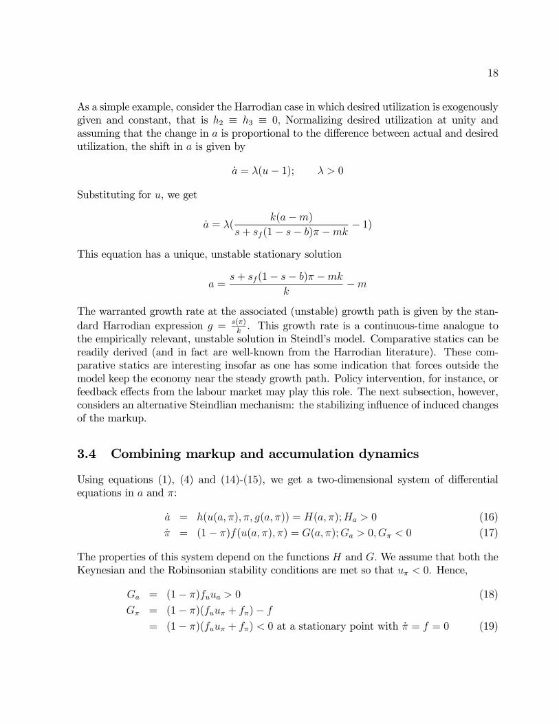
3.4 Combining markup and accumulation dynamics

Using equations (1), (4) and (14)-(15), we get a two-dimensional system of differentialequations in a and π:

a = h(u(a, π), π, g(a, π)) = H(a, π);Ha > 0 (16)

π = (1− π)f(u(a, π), π) = G(a, π);Ga > 0, Gπ < 0 (17)

The properties of this system depend on the functions H and G.We assume that both theKeynesian and the Robinsonian stability conditions are met so that uπ < 0. Hence,

Ga = (1− π)fuua > 0 (18)

Gπ = (1− π)(fuuπ + fπ)− f

= (1− π)(fuuπ + fπ) < 0 at a stationary point with π = f = 0 (19)

19

Turning to the partials of H, we have

Ha = huua + hgga > 0 (20)

Hπ = huuπ + hπ + hggπ (21)

The first term in the expression for Ha is positive and the second negative. In line with thediscussion in subsection 3.3, however, we assume that the first term will dominate and thatthe pure accumulation dynamics is destabilizing; that is, we consider the case in whichHa > 0. The partial Hπ, on the other hand, is difficult to sign on either theoretical orempirical grounds. As a result, qualitatively diverse dynamic scenarios are possible.

In terms of the reduced forms H and G, the Jacobian of the system is given by

J(a, π) =

µHa Hπ

Ga Gπ

¶and the stationary point is locally stable if (evaluated at the stationary point) we have

Det(J) = HaGπ −GaHπ > 0

Tr(J) = Ha +Gπ < 0

Saddlepoint instability is obtained if Det(J) < 0, and the system generates an unstablenode or focus if Det(J) > 0 but Tr(J) < 0.

In Appendix B we illustrate these possibilities. One case allows for a stable steady growthpath and generates roughly Steindlian results. This case demonstrates that a system whichhas an unstable equilibriumwhen the markup is exogenous may be stabilized by endogenouschanges in the markup, provided the adjustments of the markup are sufficiently fast. Asecond case (also based on assumptions that seem plausible a priori) implies saddlepointinstability. This case shows that fast adjustment in the markup may not suffice to stabilizethe system. Both cases are characterized using assumptions concerning the underlyingfunctions f, g and h.17

The phase diagram in figure 2 depicts the dynamics when the system (16)-(17) generatesa node or a focus and, assuming stability, the figure can be used to examine the effectsof changes in competition. According the Steindl, a decline in competition puts upwardpressure on the markup and, secondly, leads to a decline in the adjustment speed of themarkup. The first effect corresponds to an upward shift in the Phillips curve (the f -function) while the second can be parameterized by introducing a multiplicative constantµ in the equation for the change in the profit share. Thus, the effects of changes in thedegree of competition can be captured by re-writing equation (17) as

π = (1− π)µ [f(u(a, π), π) + ν] = G(a, π;µ, ν)

17The two cases do not exhaust the set of possibilities with respect to these underlying functions.

20

Figure 2: Stabilizing markup dynamics

The benchmark degree of competition in (17) is associated with µ = 1 and ν = 0; increasedoligopolization leads to a reduction in µ (slower adjustment speeds) and a rise in ν (upwardpressure on the markup).

Consider now the effects of increased oligopolization. The rise in ν implies an upward shiftin the π = 0 locus while changes in µ have no effects on the slope or position of eitherof the two loci. The upward shift in the π = 0 locus entails a decline in the stationarysolutions of both a and π (see figure 2), and the rates of utilization and accumulation mustfall too. To see this, note that by assumption fπ ≤ 0, and the rise in ν must therefore beassociated with a decline in u if f(u, π) + ν is to remain equal to zero. The fall in the rateof accumulation now follows from the decline in both u and π (since g = s(π)

ku).

Although changes in the parameter µ have no effects on the shapes and positions of theπ = 0 and a = 0 loci, these changes may still be of critical importance. By assumption thepure accumulation dynamics is unstable (Ha > 0), and there is therefore a critical valueµ such that Tr R 0 for µ S µ. It follows that a decline in competition may destabilize apreviously stable equilibrium.

Overall then, assuming stability of the stationary solution, the Steindlian system (16)-(17) with the restrictions (18)-(20) implies that increased oligopolization will (i) produce adecline in the equilibrium values of utilization and the rate of accumulation, and (ii) endan-ger the local stability of the equilibrium. These implications are consistent with Steindl’sconclusions. But somewhat surprisingly - and contrary to Steindl’s analysis - increased

21

oligopolization (an upward shift in the price Phillips curve) ultimately generates a fall inthe profit share.18 Of course, one could re-define increased oligopolization as a rise in themarkup, rather than an upward shift in the price Phillips curve. This alternative definitionevades the paradox but produces an un-Steindlian positive relation between oligopolizationand growth. In any case, the paradoxical rise in the profit share following an upward shiftin the price Phillips curve is reversed when we add reserve-army effects.

4 Adding a labour market

4.1 The reserve army of labour

The dynamic systems developed so far have focused on the product market and the inter-action between investment, saving, finance and pricing decisions. The neglect of the labourmarket is striking but not entirely un-Steindlian. Steindl (1952, p. 168) for instance pointsout that, since it is strongly influenced by immigration, the growth of the working popula-tion is as much an effect as a cause of the trend in accumulation. The same conclusion isreached in his discussion of Marx on pp. 233-34. According to this position, the growthof the labour force is endogenous and does not constrain accumulation.

It is hard to square this dismissal of any role of the labour supply with Steindl’s (1979,p. 12) argument that “the most striking feature of the new economic climate” is the wayprolonged near-full employment “has strengthened the economic position of workers andthe power of trade unions, and has led to demands for workers’ participation”. As a resultof these demands, he argues, the attitudes of governments and big business alike havechanged:

Formerly there was a general conviction in most countries that the governmentwould intervene to prevent a prolonged depression; this reduced uncertainty andtherefore made for higher and more stable private investment. This confidencehas been shattered. Here is another reason why the function φ [the investmentfunction] has shifted downwards (1979, p. 13)

Steindl’s seemingly contradictory suggestions with respect to labour market conditions maybe reconciled by noting that although there have been periods of low official unemployment

18This paradoxical result is in line with Dumenil and Levy’s (1996) data on US trends in profitabilityafter the civil war. Steindl, who did not have profit data for this period, argued that “towards the endof the last century ... the American economy had undergone a transition which gave considerable weightto the oligopolistic pattern in the total economy” (p. 191). He suggested that this transition would haveraised profit margins. According to Dumenil and Levy’s data, however, the profit share declined at anaverage annual growth rate of 0.4 percent between 1869 and 1910.

22

both before the big depression and in the 1950s and 1960s, the supply of labour to themodern, capitalist part of the economy was quite elastic. Up until the 1960s most OECDcountries had hidden reserves of unemployment in agriculture, in parts of the service sec-tor and among women, and, as pointed out by Steindl, immigration also helped alleviateany shortages of labour. The hidden reserve army gradually became depleted, however,and immigration was hampered by growing political resistance. As a result, the economybecame mature in Kaldor’s (1966) sense of the word: its growth rate became constrainedby the growth in the labour force.

We formalize this argument (which may or may not be a reasonable representation ofSteindl’s thinking) by including an effect of labour market conditions on the shifts in theinvestment function. Thus, let

a = h(u(a, π), π, g(a, π), e); h1 > 0, h2 ≥ 0, h3 ≤ 0, h4 < 0= H(a, π, e) (22)

where e is the measure of labour market conditions. We shall refer to this variable simplyas the employment rate. In any empirical application, however, the role of hidden unem-ployment as well as the possibility of obtaining workers through immigration must be takeninto account. The equation describes how ‘animal spirits’ suffer under full employment,leading to a gradual, downward shift in the investment function. These employment effectsare likely to be non-linear: negligible at high levels of unemployment but very substan-tial when the economy approaches full employment. Equation (22) captures, we believe,Steindl’s main point - a point which is closely related to Kalecki’s (1943) insights thatpersistent high employment undermines “the social position of the boss” and “the self as-surance and class consciousness of the working class” grows (quoted from Kalecki (1971, p.140-1).

The movements in the employment rate depend on changes in the labour force, output andtechnology. Assuming Harrod-neutral technical progress, we have

e = e(u+ g − n)

= e

∙ua(a, π)

u(a, π)a+

uπ(a, π)

u(a, π)π + g(a, π)− n

¸(23)

where n is the growth rate of the labour force in efficiency units. For simplicity we shallignore the possibility of induced changes in the growth of the labour supply and take n tobe constant.

4.2 Employment and accumulation dynamics

Equations (22)-(23) and (17) constitute a three-dimensional system in a, π, e. First, how-ever, we shall consider the special case with a constant markup, that is, the case in which

23

π ≡ 0. We then have the following two-dimensional systema = H(a, e);Ha > 0, He < 0

e = e

∙ua(a)

u(a)a+ g(a)− n

¸= F (a, e)

where it is assumed, as in section 3, that the pure accumulation dynamics is unstable(Ha > 0).

At a stationary point we get

Fa = e

∙ua(a)

u(a)Ha + g0(a)

¸> 0 since g0(a) > 0,

ua(a)

u(a)> 0, Ha > 0

Fe = eua(a)

u(a)He < 0

Hence, evaluated at a stationary point, the Jacobian takes the following form

J(a, e) =

ÃHa He

ehua(a)u(a)

Ha + g0(a)i

eua(a)u(a)

He

!and

Det(J) = −eg0(a)He > 0

Tr(J) = Ha + eua(a)

u(a)He

It follows that the stationary solution represents a node or a focus. Unlike the system withmarkup and accumulation dynamics, saddlepoint instability can be excluded. But analo-gously to the case of a node/focus in section 3.4, stability is ensured if animal spirits adjustslowly relative to the adjustment in the stabilizing variable, in this case the employmentrate. A Marxian reserve army effect, in other words, may help to stabilize the economy.

4.3 Employment, accumulation and markup dynamics

Now consider the full three dimensional system consisting of (22)-(23) and (17). Ifgπ(a, π) ≥ 0, there is (at most) one stationary solution.19 To see this, note that stationarityrequires

g(a, π) = n; ga > 0, gπ ≥ 0G(a, π) = 0; Ga > 0, Gπ < 0

19Without the restriction gπ ≥ 0 there may (but need not) be multiple solutions. The restriction issatisfied in the special case analyzed by Dutt (1995) - who assumes g = a and gπ = 0 - as well as by allexhilirationist cases.

24

These two equations cannot have more than one solution for a∗ and π∗. Having found a∗, π∗,the equilibrium solution for the employment rate can be derived from

a = H(a∗, π∗, e) = 0;He < 0

Evaluated at a stationary point the Jacobian of the three-dimensional system takes thefollowing form

J(a, π, e) =

⎛⎝ Ha Hπ He

Ga Gπ 0e(ua

uHa +

uπuGa + ga) e(ua

uHπ +

uπuGπ + gπ) eua

uHe

⎞⎠The necessary and sufficient Routh-Hurwitz conditions for local stability are that

1. Tr(J) = Ha +Gπ + euauHe < 0

2. Det(J1) +Det(J2) +Det(J3) = eHe[uauGπ − uπ

uGa − ga] +HaGπ −GaHπ > 0

3. Det(J) = eHe[gπGa − gaGπ] < 0

4. −Tr(J)[Det(J1) +Det(J2) +Det(J3)] +Det(J) > 0

The second condition will be satisfied if the stabilizing effect of the reserve army is suffi-ciently strong (that is, for sufficiently large absolute values of He). To see this, note thatusing (18)-(19) the term in square brackets can be written

uauGπ − uπ

uGa − ga =

uau(1− π)fπ − ga

Since ua > 0, fπ ≤ 0 and ga > 0 the right hand side of this equation is unambiguouslynegative.

The third condition is satisfied if the expression in the square brackets is positive and,when combined with the signs of the other partials, our earlier condition for uniqueness(gπ ≥ 0) is sufficient to ensure that this is the case. If the second and third conditions aremet, finally, the first and fourth will also hold if the absolute value of He is large. To seethat the fourth condition will be met, note that −Tr(J)[Det(J1) +Det(J2) +Det(J3)] isquadratic in He while Det(J) is linear.

It may be interesting to look briefly at the comparative statics of increasing oligopolizationfor the three-dimensional systems. Increasing oligopolization corresponds to an upwardshift in the G(a, π)-equation that describes the mark-up dynamics. We have Ga > 0 andGπ < 0, and this upward shift therefore has to be offset by an increase in π and / or adecline in a. Since the long-run rate of growth g(a, π) must remain equal to n and sinceby assumption ga > 0 and gπ ≥ 0, it follows that a and π cannot move in the same

25

direction. Thus, π must increase while the change in a must be non-positive. Utilization,which is increasing in a but decreasing in π, therefore must fall. The effect on employment,finally, can be found from the stationarity condition for a: h(u, π, g, e) = 0. Since g = n isunchanged we have

0 = hu(uada+ uπdπ) + hπdπ + hede

or

de =[hu(uada+ uπdπ)] + hπdπ

−heThe denominator of the expression on the right hand side is positive and it follows that em-ployment falls iff the numerator is negative. The term in square brackets is unambiguouslynegative and, as argued above, desired utilization is likely to be very insensitive to changesin profitability; that is, hπdπ will be small. Thus, although a positive employment effectcannot be ruled out, the most likely outcome is one where increasing oligopolization leadsto a rise in unemployment. Intuitively, a larger reserve army is needed to boost animalspirits in order to make up for the depressing effects of lower utilization.20 These effects,are consistent with Steindl’s predictions: increased oligopolization raises the profit sharebut generates stagnation in the form of lower employment and capital utilization.

The long-term effects of a transition, finally, from a stage of large hidden unemployment(in which hg = 0) to one of Kaldorian maturity may be analyzed by comparing a stationarypoint of the two-dimensional accumulation-mark-up dynamics (with g > n) to a stationarypoint of the three-dimensional system. But for the comparison to be meaningful, it must beassumed that the stationary points are stable, and the case of saddlepoint instability in thetwo-dimensional system is therefore excluded. Assuming that initially we are in the stabletwo-dimensional case, the negative effect of the employment rate on the rate of change ofanimal spirits as the economy reaches a mature stage can be depicted as a rightward shiftof the a = 0 locus in figure 2. The result is a decline in both a and π. The rate of utilizationthen must fall (or, if fπ = 0, remain unchanged).21 Thus, the transition to a new stationarypoint associated with a constant employment rate implies a fall in the rate of accumulationto bring it into line with the growth of the labour force (g = n), and a decline in both therate of utilization and the profit share.

20These results mirror the effects obtained by Skott (1989a, pp. 151-153). In Skott’s Marshallian setting,changes in output are related to the difference between realized and target profit margins and, by raisingthe target, increased monopolization therefore depresses output for any given realized profit margin.21To see this, observe that f(u, π) = 0 at the stationary solution. Total differentiation yields fudu +

fπdπ = 0, and the result now follows from fu > 0, fπ ≤ 0.

26

5 Conclusions and extensions

We opened this paper by comparing a standard Steindl-Kalecki model with Steindl’s (1952)analysis. This comparison revealed several differences, and both the standard model andSteindl’s own formalization had significant weaknesses, we argued. Steindl himself noteda puzzling and unsatisfactory aspect of his model: it generated unreasonably high valuesof the (locally) stable steady-state solutions for utilization and the rate of growth. Onecontribution of this paper is to demonstrate that weak and questionable non-linearities liebehind this problematic feature of his model. The main contribution, however, lies in thepresentation and analysis of extended Steindlian models that address the weaknesses of thestandard model.

Using a continuous-time framework, we first incorporated the interaction between markupdynamics and accumulation dynamics. Steindl, more than any other contributor to thepost Keynesian tradition, has emphasized the influence of competitive conditions on thesensitivity of the markup to changes in utilization, and he has consistently combined thisemphasis with a keen awareness of the possibilities of Harrodian instability arising fromstrong, lagged effects of utilization on the rate of accumulation. In our view the dy-namic interaction between accumulation and the markup therefore constitutes the core ofa Steindlian model.

We formalized the interaction between markup dynamics and accumulation dynamics inthe form of a two-dimensional system of differential equations, one for shifts in the markupand one for shifts in ‘animal spirits’. Consistent with Steindl’s vision, we find that fastadjustment of the markup may (but need not) contribute to a stabilization of the steadygrowth path. The model also supports Steindl’s position on the stagnationist effects ofincreased oligopolization: an upward shift in the dynamic equation for the markup generatesa decline in both utilization and growth. Paradoxically, however, in the stable case it alsoleads to a decline in the stationary solution for the markup.

The core model - developed in section 3 - can be extended in various ways. Our extensionin section 4 focuses on the Marxian influence of the reserve army. There is a tension inSteindl’s views on this issue. Steindl (1952) largely dismisses the idea that accumulationcould be constrained by a declining reserve army. In Steindl (1979), however, his positionon this issue appears to have changed since in this paper the effect of prolonged near-fullemployment on accumulation plays a key role. In any case, the inclusion of a reservearmy effect tends to stabilize the economy (as in Skott (1989a, 1989b)), and the effectsof increasing oligopolization are quite Steindlian: increasing oligopolization must leave thegrowth rate unchanged - since it is tied to the growth of the labour force in this model - butoligopolization has stagnationist effects in the form of a fall in both the employment rateand the rate of capital utilization. It should be noted also that in this three dimensionalsystem, which incorporates employment dynamics as well as markup and accumulationdynamics, an upward shift of the dynamic equation for the markup raises the stationary

27

value of the markup. Thus, the paradox that characterizes the two-dimensional systemwithout a labour market disappears in the extended system.

Our extensions of the standard model capture, we believe, important Steindlian insightsand overcome some shortcomings of earlier formalizations. But our extended models clearlyhave weaknesses and limitations. Financial factors, for instance, play a very limited role.We have allowed for retained earnings to stimulate investment. The ‘principle of increasingrisk’ - the cost and riskiness of high degrees of external finance - may provide a rationale forthe role of retained earnings. But with a constant retention rate, retained earnings mightalso appear in the investment function simply because high current profitability signalsthe profitability of additions to the capital stock. Furthermore, the principle of increasingrisk suggests that in terms of financial constraints, the gearing ratio rather the flow ofretained profits may be the more important variable. Thus, following Steindl (1952), onemay extend the model by including the gearing ratio in the investment function.22 Thegearing ratio, indeed, is a key variable in Dutt’s (1995) examination of the interactionbetween the product market and financial aspects. His analysis, which leaves out markupdynamics and labor market effects, can be seen as complementary to the one presented inthis paper.

Other prominent aspects of Steindl’s verbal analysis also suggest further extension of themodel. We have taken all saving rates as well as firms’ financial environment as constant.These assumptions could be relaxed to allow for the presence of stock markets and capitalgains as well as endogenous changes in saving behaviour (emphasized by Steindl in severalcontributions, e.g. Steindl (1982)), the effects of institutional influences on saving (e.g.Pitelis (1997)) or evolving standards of financial behaviour along the lines suggested byMinsky (e.g. Steindl (1990 [1989], p. 173)). From an applied perspective, however, the mostsevere shortcomings probably arise from the neglect of policy, both fiscal and monetary,and the closed-economy assumption. Thus, the possibility of export and profit led growthclearly increases in an open economy setting (e.g. Blecker (1989) and Bhaduri and Marglin(1990)). We leave extensions in these and other directions for future research.

6 Appendices

6.1 Appendix A

Let

f(u) =mk

s(u− 11 + su

);u ≥ 022These financial aspects are left out in Steindl (1979). This more recent analysis instead emphasizes

labour market effects and markup dynamics, although neither of these factors are included in the formalequations.

28

The function f(u) is increasing and strictly concave: f 0(u) > 0, f 00 < 0. Furthermore,

f(u) R 0 for u R 1

f(u) → mk

s

1

sfor u→∞

Hence, u > f(u) both when u is small and when u is sufficiently large. The inequality,however, may be reversed for intermediate values of u. Since f(u) < mk

su for all u, however,

the parameter restriction mks> 1 is a necessary condition for this to happen.

6.2 Appendix B

A stable case: Assume that

• current accumulation depends non-negatively on profitability, that the change in adepends negatively on the current growth rate, and that there are no direct effects ofprofitability on the change in a; that is hg < 0, hπ ≡ 0 and gπ ≥ 0.

• Price inflation is completely insensitive to small variations in the profit share in theneighborhood of the stationary point; that is fπ ≡ 0 in this neighbourhood.

• market conditions are competitive in the Steindlian sense that adjustments in themarkup are sensitive to deviations of actual utilization from desired utilization. More-over, the speed of markup adjustment is fast relative to shifts in the accumulationfunction (fu >> hu).

Using the first two assumptions, we get

dπ

da |π=0= −Ga

Gπ=

ua−uπ >

ua +hghuga

−uπ − hghugπ= −Ha

Hπ=

dπ

da a=0> 0

It follows that the π = 0 locus is steeper than the a = 0 locus and, using (17)-(19), thatDet(J) > 0. Thus, assuming the existence of a stationary solution, the stationary pointmust be a node or a focus. Furthermore, the third assumption on the relative adjustmentspeeds of a and π ensures that the second stability condition will also be met. To see this,note that

Tr(J) = Ha +Gπ = huua + [hgga + (1− π)fuuπ]

The term in square brackets in the expression for the trace is negative while the first termis positive. Stability - quite intuitively - can be undermined if the destabilizing adjustmentsof investment function are fast relative to the speed of stabilizing markup adjustment.

A saddlepoint: Our second case shows that fast price adjustments will not always sufficeto stabilize the system. Assume that

29

Figure 3: Saddlepoint dynamics; 3a: Hπ > 0; 3b: Hπ < 0

• There is no negative feedback from the current accumulation rate to the change in a(that is, hg = 0)

• The profit share exerts a positive effect on the change in a and/or a direct negativeeffect on price inflation (hπ > 0 and/or fπ < 0)

It is readily seen that with these assumptions the determinant of the Jacobian becomesnegative and the stationary point is a saddlepoint. Figures 3a and 3b illustrate the outcome.In figure 3a, Hπ > 0 and the a = 0 locus is negatively sloped. In figure 3b, Hπ < 0, andboth loci are positively sloped; the slope of the a = 0 locus, however, is steeper than thatof the π = 0 locus. In both figures the stationary point exhibits saddlepoint instability,and global analysis is needed to decide what will happen over the longer run.

References

[1] Amadeo, E. (1986) “The role of capacity utilization in long-period analysis”. PoliticalEconomy, 2 (2), pp. 147-185.

[2] Auerbach, P. (1988) Competition. Oxford: Blackwell.

[3] Auerbach, P. and Skott, P. (1988) "Concentration, competition and distribution".International Review of Applied Economics, 2, pp. 42-61.

30

[4] Blecker, R. (1989) “International competition, income distribution and economicgrowth”. Cambridge Journal of Economics, 14, pp. 375-393.

[5] Dumenil, G. and Levy, D. (1996) “The acceleration and slowdown of technical progressin the US since the civil war”. Revue Internationale de Systemique, 10 (3), pp. 303-321.

[6] Dutt, A.K. (1984) "Stagnation, income distribution and monopoly power". CambridgeJournal of Economics, 8, pp. 25-40.

[7] Dutt, A.K. (1992) “Conflict inflation, distribution, cyclical accumulation and crises”European Journal of Political Economy, 8, pp. 579-597.

[8] Dutt, A.K. (1995) "Internal finance and monopoly power in capitalist economies: areformulation of Steindl’s growth model". Metroeconomica, 46:1, pp. 16-34.

[9] Dutt, A.K. (1997) “Equilibrium, path dependence and hysteresis in post-Keynesianmodels”. In P. Arestis, G. Palma and M. Sawyer (eds) Capital Controversy, Post-Keynesian Economics and the History of Economic Thought: Essays in Honour ofGeoff Harcourt, London: Routledge.

[10] Flaschel, P. and Krolzig, H.-M. (2003) "Wage and price Phillips curves. An empiricalanalysis of destabilizing wage-price spirals". Working paper: Oxford University.

[11] Goodwin, R.M. (1967) “A growth cycle”. In C.H. Feinstein (ed.) Socialism, capitalismand growth, Cambridge: Cambridge University Press.

[12] Kaldor, N. (1996) Causes of the slow rate of economic growth in the United Kingdom.Cambridge: Cambridge University Press.

[13] Kalecki, M (1943) "Political aspects of full employment". Reprinted in M. Kalecki,Selected essays on the dynamics of the capitalist economy, Cambridge: CambridgeUniversity Press, 1971.

[14] Kalecki, M. (1954) Theory of economic dynamics. London: Allen & Unwin.

[15] Kurz, H. (1986) “Normal positions and capital utilization”. Political Economy, 2 (1),pp. 37-54.

[16] Lavoie, M. (1995) “The Kaleckian model of growth and distribution and its neo-Ricardian and neo-Marxian critiques”. Cambridge Journal of Economics, 19, pp. 789-818.

[17] Levy, D., Bergen, M., Dutta, S. and Venable, R. (1997) “The magnitude of menu costs:direct evidence from large U.S. supermarket chains”. Quarterly Journal of Economics,112, pp. 791-825.

31

[18] Marglin, S.A. and Bhaduri, A. (1990) "Profit squeeze and Keynesian theory". In S.A.Marglin and J.B. Schor (eds) The golden age of capitalism, Oxford: Clarendon Press.

[19] Pitelis, C. (1997) “On Kaldor and pensions”. Cambridge Journal of Economics, 21(4):469-482,

[20] Robinson, J. (1962) Essays in the Theory of Economic Growth. London and Bas-ingstoke: Macmillan.

[21] Rowthorn, B. (1981) "Demand, real wages and economic growth". Thames Papers inPolitical Economy.

[22] Sawyer, M. (1985)The economics of Michal Kalecki. London and Basingstoke: Macmil-lan.

[23] Sawyer, M. (1995) Unemployment, Imperfect Competition and Macroeconomics. Alder-shot: Edward Elgar.

[24] Semmler, W. (1984) Competition, monopoly and differential profit rates. New York:Columbia University Press.

[25] Skott, P. (1989a) Conflict and effective demand in economic growth. Cambridge: Cam-bridge University Press.

[26] Skott, P. (1989b) "Effective demand, class struggle and cyclical growth". InternationalEconomic Review, 30, pp. 231-247.

[27] Steindl, J. (1952)Maturity and stagnation in American capitalism. Oxford: Blackwell.

[28] Steindl, J. (1979) "Stagnation theory and stagnation policy". Cambridge Journal ofEconomics, 3, pp. 1-14.

[29] Steindl, J. (1982) "The role of household saving in the modern economy". BancaNazionale del Lavoro Quarterly Review. Reprinted in Steindl (1990).

[30] Steindl, J. (1989) "From stagnation in the 30s to slow growth in the 70s". In M. Berg(ed.) Political economy in the twentieth century, Oxford: Philip Allan. Reprinted inSteindl (1990).

[31] Steindl, J. (1990) Economic Papers 1941-88. London and Basingstoke: Macmillan.

[32] Taylor, L. (1985) "A stagnationist model of economic growth". Cambridge Journal ofEconomics, 9, pp. 383-403.