Embed Size (px)
Citation preview

A Python-PSSE-Based WECC Composite Load Parameter
Identification Tool
Dr. Yingmeng XiangMr. Zixiao Ma
Prof. Zhaoyu WangIowa State University
July 2021
Department of Electrical and Computer Engineering

Contents
2
• Background and motivation
• Introduction of the parameter identification approach
• Identification of WECC composite load model using AEP data
ECE Department

3
ECE Department
WECC composite load model (CMPLDW) Transformer and feeder contain
18 parameters Three phase motors contain 65
parameters Single phase motor contains 34
parameters Electronic load contains 5
parameters Static load contains 11
parameters DG contains 46 parameters
(currently unmodeled in the PSSE WECC model)
A highly nonlinear and complex load model
Objective: Using event data to identify the parameters of WECCcomposite load model to fit the active and reactive powermeasurements.

ECE Department
Problem description
Challenges:Large nonlinear searching space (133 parameters need to beidentified).Establish stable connection between Python and PSSE forinformation exchange.

ECE Department
Overview of Python-PSSE autonomous parameter identification approach
Advantages: We can flexibly choose various optimization methods to efficiently
optimize the WECC parameters. The salp swarm algorithm ischosen just as an example due to its high efficiency of searching.
The playback generator model allows us to inject disturbancerecorded by real PMU data.
G L
PMU Voltage measurements
PMU frequency measurements
Playback generator model
WECC load model
Line
Salp swarm algorithmP, Q curves
PSSE environment
WECC parameters
Python environment

ECE Department
Program flowchartStart
Initialize the positions of the salp swarm
Update the WECC parameters based on the positions of the salp swarm
Call PSSE to perform dynamic simulation
Get the errors between the simulated curves and PMU measurements
Update food position based on the errors
Update the positions of the salp swarm
Satisfy termination?
EndYes
No
mi n1
2𝑁𝑁�𝑖𝑖=1
𝑁𝑁
𝑃𝑃𝑖𝑖𝑠𝑠𝑖𝑖𝑠𝑠 − 𝑃𝑃𝑖𝑖𝑃𝑃𝑃𝑃𝑃𝑃2 + 𝑄𝑄𝑖𝑖𝑠𝑠𝑖𝑖𝑠𝑠 − 𝑄𝑄𝑖𝑖𝑃𝑃𝑃𝑃𝑃𝑃
2
where: 𝑃𝑃𝑖𝑖𝑠𝑠𝑖𝑖𝑠𝑠: The simulated active power curve. 𝑃𝑃𝑖𝑖𝑃𝑃𝑃𝑃𝑃𝑃: The active power curve by PMU. 𝑄𝑄𝑖𝑖𝑠𝑠𝑖𝑖𝑠𝑠: The simulated reactive power curve. 𝑄𝑄𝑖𝑖𝑃𝑃𝑃𝑃𝑃𝑃: The reactive power curve by PMU. 𝑁𝑁: The number of measurements.

ECE Department
Parameter identification using AEP data
A fault happened on a 138 kV line. The fault event was recorded by PMU at a nearby 12.47 kV substation.
0 5 10 15 20
Time (seccond)
0.5
0.6
0.7
0.8
0.9
1
1.1
Vol
tage
(p.u
.)
0 5 10 15 20
Time (seccond)
-0.01
-0.005
0
0.005
0.01
Freq
uenc
y de
viat
ion
(Hz)
Recorded voltage curve Recorded frequency deviation curve

8
Initial CMPLDW parametersJ+index
Name Value J+index
Name Value J+ index Name Value J+index
Name Value J+index
Name Value
0 MVA -1 27 P1e 2 54 Ftr2A 0.3 81 LpC 0.19 108 Np1 11 SubstB 0 28 P1c 0.3 55 Vrc2A 0.1 82 LppC 0.14 109 Kq1 62 Rfdr 0.04 29 P2e 1 56 Trc2A 999 83 TpoC 0.2 110 Nq1 23 Xfdr 0.04 30 P2c 0.7 57 MtypB 3 84 TppoC 0.0026 111 Kp2 124 Fb 0.75 31 Pfrq 0 58 LFmB 0.75 85 HC 0.1 112 Np2 3.25 XXf 0.08 32 Q1e 2 59 RaB 0.03 86 EtrqC 2 113 Kq2 116 Tfixhs 1 33 Q1c -0.5 60 LsB 1.8 87 Vtr1C 0 114 Nq2 2.57 Tfixls 1 34 Q2e 1 61 LpB 0.19 88 Ttr1C 999 115 Vbrk 0.868 LTC 0 35 Q2c 1.5 62 LppB 0.14 89 Ftr1C 0 116 Frst 0.39 Tmin 0.9 36 Qfrq -1 63 TpoB 0.2 90 Vrc1C 999 117 Vrst 0.9510 Tmax 1.1 37 MtypA 3 64 TppoB 0.0026 91 Trc1C 999 118 CmpKpf 111 Step 0.00625 38 LFmA 0.75 65 HB 0.5 92 Vtr2C 0 119 CmpKpf -3.312 Vmin 1.025 39 RsA 0.04 66 EtrqB 2 93 Ttr2C 999 120 Vc1off 0.513 Vmax 1.04 40 LsA 1.8 67 Vtr1B 0 94 Ftr2C 0 121 Vc2off 0.414 Tdelay 30 41 LpA 0.12 68 Ttr1B 999 95 Vrc2C 999 122 Vc1on 0.6515 Tstep 5 42 LppA 0.104 69 Ftr1A 0 96 Trc2C 999 123 Vc2on 0.5516 Rcmp 0 43 TpoA 0.095 70 Vrc1B 999 97 Tstall 0.0333 124 Tth 717 Xcmp 0 44 TppoA 0.0021 71 Trc1B 999 98 Trestart 0.3 125 Th1t 0.418 FmA 0.237 45 HA 0.1 72 Vtr2B 0 99 Tv 0.025 126 Th2t 319 FmB 0.119 46 EtrqA 0 73 Ttr2B 999 100 Tf 0.1 127 Fuvr 020 FmC 0.1 47 Vtr1A 0.65 74 Ftr2B 0 101 CompLF 1 128 UVtr1 021 FmD 0.24 48 Ttr1A 0.2 75 Vrc2B 999 102 CompPF 0.98 129 Ttr1 99922 Fel 0.162 49 Ftr1A 0.3 76 Trc2B 999 103 Vstall 0.45 130 UVtr2 023 Pfel 1 50 Vrc1A 0.1 77 MtypC 3 104 Rstall 0.124 131 Ttr2 99924 Vd1 0.7 51 Trc1A 999 78 LFmC 0.75 105 Xstall 0.114 132 FrstPel 125 Vd2 0.5 52 Vtr2A 0.65 79 RaC 0.03 106 Lfadj 026 PFs 1 53 Ttr2A 0.33 80 LsC 1.8 107 Kp1 0
The initial parameters provide an acceptable initial estimation.
ECE Department

ECE Department
Selection of parameters for identification
Ideally, our approach is able to optimize all the parameters within anyrange.
However, the random selection of some parameters (such as LsA,LpA, LppA, TpoA, TppoA, HA, EtrqA, Vtr1A, Ttr1A, Ftr1A, Vrc1A) maycause the collapse of PSSE.
J+ Index Name Initial value Bound J+ Index Name Initial value Bound18 FmA 0.237 [0.0474, 0.711] 35 Q2c 1.5 [-3, 3]19 FmB 0.119 [0.0238, 0.357] 38 LFmA 0.75 [0.375, 1.125]20 FmC 0.1 [0.02, 0.3] 39 RaA 0.04 [0.02, 0.06]21 FmD 0.24 [0.048, 0.72] 58 LFmB 0.75 [0.375, 1.125]22 Fel 0.162 [0.0324, 0.486] 59 RaB 0.03 [0.015, 0.045]23 PFel 1 [0.95, 1] 78 LFmC 0.75 [0.375, 1.125]24 Vd1 0.7 [0.42, 0.77] 79 RaC 0.03 [0.015, 0.045]25 Vd2 0.5 [0.3, 0.55] 109 Kq1 6 [4.8, 9]26 PFs 1 [0.85, 1] 110 Nq1 2 [1.6, 3]28 P1c 0.3 [0.15, 1.5] 124 Tth 5 [4, 10]30 P2c 0.7 [0.35, 3.5] 125 Th1t 0.4 [0.32, 0.8]33 Q1c -0.5 [-1, 1] 126 Th2t 3 [2.4, 6]

10
ECE Department
Convergence of SSA
30 salps (parallel candidate solutions).
50 iterations. The simulation takes 39
minutes. The main computation
time is spent on the PSSE dynamic simulation and output data processing.0 10 20 30 40 50 60
Iteration number
0.46
0.48
0.5
0.52
0.54
0.56
0.58
0.6
0.62
Mea
n sq
uare
root
erro
r (M
W)
11
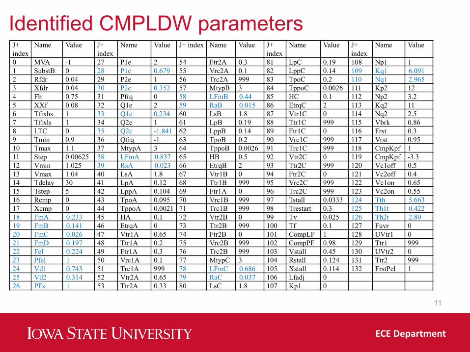
J+index
Name Value J+index
Name Value J+ index Name Value J+index
Name Value J+index
Name Value
0 MVA -1 27 P1e 2 54 Ftr2A 0.3 81 LpC 0.19 108 Np1 11 SubstB 0 28 P1c 0.679 55 Vrc2A 0.1 82 LppC 0.14 109 Kq1 6.0912 Rfdr 0.04 29 P2e 1 56 Trc2A 999 83 TpoC 0.2 110 Nq1 2.9653 Xfdr 0.04 30 P2c 0.352 57 MtypB 3 84 TppoC 0.0026 111 Kp2 124 Fb 0.75 31 Pfrq 0 58 LFmB 0.44 85 HC 0.1 112 Np2 3.25 XXf 0.08 32 Q1e 2 59 RaB 0.015 86 EtrqC 2 113 Kq2 116 Tfixhs 1 33 Q1c 0.234 60 LsB 1.8 87 Vtr1C 0 114 Nq2 2.57 Tfixls 1 34 Q2e 1 61 LpB 0.19 88 Ttr1C 999 115 Vbrk 0.868 LTC 0 35 Q2c -1.841 62 LppB 0.14 89 Ftr1C 0 116 Frst 0.39 Tmin 0.9 36 Qfrq -1 63 TpoB 0.2 90 Vrc1C 999 117 Vrst 0.9510 Tmax 1.1 37 MtypA 3 64 TppoB 0.0026 91 Trc1C 999 118 CmpKpf 111 Step 0.00625 38 LFmA 0.837 65 HB 0.5 92 Vtr2C 0 119 CmpKpf -3.312 Vmin 1.025 39 RsA 0.023 66 EtrqB 2 93 Ttr2C 999 120 Vc1off 0.513 Vmax 1.04 40 LsA 1.8 67 Vtr1B 0 94 Ftr2C 0 121 Vc2off 0.414 Tdelay 30 41 LpA 0.12 68 Ttr1B 999 95 Vrc2C 999 122 Vc1on 0.6515 Tstep 5 42 LppA 0.104 69 Ftr1A 0 96 Trc2C 999 123 Vc2on 0.5516 Rcmp 0 43 TpoA 0.095 70 Vrc1B 999 97 Tstall 0.0333 124 Tth 5.66317 Xcmp 0 44 TppoA 0.0021 71 Trc1B 999 98 Trestart 0.3 125 Th1t 0.42218 FmA 0.233 45 HA 0.1 72 Vtr2B 0 99 Tv 0.025 126 Th2t 2.8019 FmB 0.141 46 EtrqA 0 73 Ttr2B 999 100 Tf 0.1 127 Fuvr 020 FmC 0.026 47 Vtr1A 0.65 74 Ftr2B 0 101 CompLF 1 128 UVtr1 021 FmD 0.197 48 Ttr1A 0.2 75 Vrc2B 999 102 CompPF 0.98 129 Ttr1 99922 Fel 0.224 49 Ftr1A 0.3 76 Trc2B 999 103 Vstall 0.45 130 UVtr2 023 Pfel 1 50 Vrc1A 0.1 77 MtypC 3 104 Rstall 0.124 131 Ttr2 99924 Vd1 0.743 51 Trc1A 999 78 LFmC 0.686 105 Xstall 0.114 132 FrstPel 125 Vd2 0.314 52 Vtr2A 0.65 79 RaC 0.037 106 Lfadj 026 PFs 1 53 Ttr2A 0.33 80 LsC 1.8 107 Kp1 0
Identified CMPLDW parameters
ECE Department
12
ECE Department
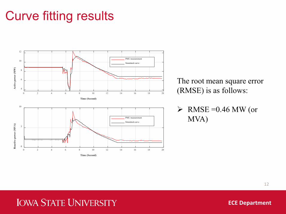
Curve fitting results
The root mean square error (RMSE) is as follows:
RMSE =0.46 MW (or MVA)
0 2 4 6 8 10 12 14 16 18 20
Time (Second)
4
6
8
10
12
Act
ive
pow
er (M
W)
PMU measurement
Simulated curve
0 2 4 6 8 10 12 14 16 18 20
Time (Second)
0
5
10
Rea
ctiv
e po
wer
(MV
A)
PMU measurement
Simulated curve

13
Thank you!
ECE Department

July 27,2021
Nick HattonStaff Engineer
WECC Base Case Data Checks

Types of data checks
Power Flow – case assembly• Data correction scripts
Dynamics data checks• Scripts (pumpcheck) • Dynamics adjustments/tests
Post assembly data checks• Steady State Dynamics Dashboard
o Power Flowo Dynamics (MVS)o NERC Case Quality Metrics
2

Power Flow – Case Assembly
bus type check Branch status and X value, branch area Transformer status, type, controlled voltage Phase shifter (control range, impedance table) Generator status, Pgen, Area, in service on islanded bus Load (status, IPLOD populated, area) Shunt (duplicate, status) SVD (generating MW?, many steps, B value, negative Vband, Area) Interchange issues Blank IDs
3

Power Flow – Case Assembly continued
Island check, bus area, Vsched = 0, bus type Gens – missing bus, Prf/Qrf = 0, reg bus = 0, Area = 0 Load – no bus, negative load with ID !=nt, area Shunt – no bus, area SVD – no bus, area Branch – 0 bus, 0 section, ohms flag = 1 Transformer – tap/control max/min = 0, change sign, change tert taps if needed Owner 0 adjustment Various other data adjustments Use DCHK in PSLF, correct some issues.
4

Dynamics Data checks
Pumpcheck – comment PSS/Gov depending on if a unit is condensing or pumping
Initialize case – check for errors. Adjust Vschedule or Pgen as needed
Run Disturbances, hunt for generators oscillating or outside acceptable ranges. correct PF, comment model, or net as needed
5

Post Assembly data checks
Steady State and Dynamics Dashboard (SADD)• Created by stakeholders, runs in Power World• Data is broken into sections
o Case errors – specified by stakeholders in WECC System Review Subcommittee (SRS). These are data points that are wrong
o Power Flow metrics – missing models, missing data points, other issues identified in SRS to be flagged and checked
o Exceeded limits – Overloadso NERC case quality metrics o Dynamics checks – data points identified as being potentially incorrect by the WECC
Modeling and Validation Subcommittee (MVS)
6

SADD example
7

July 27,2021
Kent BoltonSr Staff Engineer
WECC Generator Testing Data Checks

Gen Test Data checks
Power Flow• Use most recent Operating Case• Verify generating unit is represented in power flow, status is on, and Pgen
is near Pmax Dynamics
• Make sure all dynamic models are listed on WECC Approved Dynamic Model Library
• Run in-house data checking routine to check for gross errors in models• Read dynamic models into PSLF program• Initialize and check for errors identified by built-in data checker
10

Gen Test Data checks (cont.)
Dynamics (cont.)• Run no-disturbance simulation• Run a ringdown simulation (insertion of Chief Joseph 1400 MW Braking
Resistor)
11

© 2021 Electric Power Research Institute, Inc. All rights reserved.w w w . e p r i . c o m
PSLF/PSCAD comparison of the phasor modelLMWG Meeting July 2021
Parag Mitra (Technical Leader)Lakshmi Sundaresh (Sr. Engineer)

© 2021 Electric Power Research Institute, Inc. All rights reserved.w w w . e p r i . c o m2
What are the different models for residential HVACs?PSCAD/EMTDC Model Phasor Model Performance Model
1. Complete flux dynamics at both high and low slip
2. Load torque modeled as a crank shaft position and speed dependent quantity, good approximation at and near operational speeds
3. Single phase model can capture the effect of point on wave and unbalance
4. Skin effect on rotor bars.5. Has been validated by lab measurements
1. Complete flux dynamics good at low slip and ok at high slip
2. Load torque modeled as constant or speed dependent
3. Positive sequence model assumes balanced voltage
4. Has been validated by lab measurementsMotorc (PSLF) and INDMOT1P (Powerworld)
1. Algebraic model based on laboratory testing of numerous HVACs
2. Easy to understandMotorD or LD1PAC (PSLF)
What level of details in the HVAC model will benefit transmission planning studies the most?
© 2021 Electric Power Research Institute, Inc. All rights reserved.w w w . e p r i . c o m3
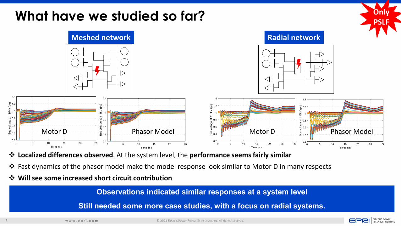
What have we studied so far?Meshed network Radial network
Observations indicated similar responses at a system level
Still needed some more case studies, with a focus on radial systems.
Motor D Phasor Model Motor D Phasor Model
Localized differences observed. At the system level, the performance seems fairly similar Fast dynamics of the phasor model make the model response look similar to Motor D in many respects Will see some increased short circuit contribution
Only PSLF

© 2021 Electric Power Research Institute, Inc. All rights reserved.w w w . e p r i . c o m4
The next phase Compare the responses of the different HVAC models for a radial system
– Electromagnetic transient model (SPIM –PSCAD model)
– Dynamic phasor model (motorc/mot1ph/ind1mot model)
– Algebraic model (ld1pac model )
Study the effect that point on wave of fault inception in the transmission/sub-transmission will have on the HVACs in the distribution system?
Is one modeling approach better than another and what should we pursue?
Are we missing any important dynamics of the HVACs

© 2021 Electric Power Research Institute, Inc. All rights reserved.w w w . e p r i . c o m5
Test Feeder model Feeder model details• 2 Three phase motors • 24 single phase motors (PSCAD)• 6 single phase phasor motor models (PSLF)• 8 static loadsThe total active power load is 35.3 MW
In PSLF we converted the 1-phase motor load at the 3-phase node to motorc.
X MW motorc in PSLF mean 3 X/3 MW motors in PSCAD connected on A, B and C respectively
Model parameterized using formula given in the documentation

© 2021 Electric Power Research Institute, Inc. All rights reserved.w w w . e p r i . c o m6
Test waveforms for the studyCase Voltage
Dip (5 cycles)Initial Voltage Recovery(4 sec)
Final Voltage recovery(2 sec)
Case 1 45%Ramped increase to 70% Ramped increase to Pre-
disturbance levelCase 2 50%
Case 3 55%
Case 4 45% Sustained at 65%
Point on wave of phase A (PSCAD only)
Dip (5 cycles) Recovery (4 sec) Final (2 sec)
0 degree (rising)45%, 50%,
55% 70% Pre-disturbance 45 degree (rising)
90 degree (peak)
V source
Case 1 - 3
Case 4

© 2021 Electric Power Research Institute, Inc. All rights reserved.w w w . e p r i . c o m7
Result Summary
Case PSCAD model(H=0.1)
PSCAD model (H=0.05)
PSLF phasor model (H=0.04)(MOTORC)
LD1PAC/MOTORDVstall-Tstall curve
LD1PAC/MOTORDVstall 0.46 Tstall 0.033s
Case 1 (45% dip)
Stalled(All 24 motors)
Stalled(All 24 motors)
Stalled Stalled Stalled
Case 2(50% dip)
Not Stalled 18 motors stalled (Phase A,Phase B)
Stalled Stalled 4 motors stalled (4*3=12 in PSCAD Equivalent)
Case 3(55% dip)
Not Stalled 2 motors stalled (Phase B)
Not Stalled Stalled Not Stalled
Case 4(45% dip)
Not Stalled 18 motors stalled (Phase A,Phase B)
Not Stalled Stalled Stalled
EMT Model Phasor Model Performance Model

© 2021 Electric Power Research Institute, Inc. All rights reserved.w w w . e p r i . c o m8
Motorc vs LD1PAC: Effect of SC contribution
• We also observed some short circuit contribution differences between the EMT model and the phasor model as well.
• The effect of short circuit contribution is to raise the on-fault voltage at the terminal of the machine

© 2021 Electric Power Research Institute, Inc. All rights reserved.w w w . e p r i . c o m9
Some Takeaways The MotorD/LD1PAC model with Vstall-Tstall curve (Tstall=-1) shows
most motors stalling The PSCAD model with comparable inertia and MotorD/LD1PAC model
shows similar conclusions on stalling of motors. The motorC model was found to produce enough electrical torque at
55%-60% voltage to be able to reaccelerate (we will investigate this further) The P-O-W effect in the tx/sub tx did not have a significant effect on our
observations The short-circuit contribution from flux dynamics provides an on- fault
voltage increase. The effect of this needs to be explored more.

© 2021 Electric Power Research Institute, Inc. All rights reserved.w w w . e p r i . c o m10
Together…Shaping the Future of Electricity
CAISO PublicCAISO Public
Composite Load Model Sensitivity Studies
Irina Green, Senior Advisor, Regional Transmission,California ISO
NERC Load Modeling Work GroupJuly 27, 2021

CAISO Public
Composite Load Model
Page 2

CAISO Public
Composite Load Modeling
California ISO uses GE PSLF with modular version of composite load for the last two years.
Load models are by climate zones and types of feeders To create load model records, NERC Load Modeling Tool is
used Some WECC cases still have composite load data by bus, but
are transitioning to the modular version in all WECC cases Update of parameters was needed WECC updated composite load parameters in 2019, moved
from version 4B to version 5B Concern – large amount of load tripped by composite load
model with three-phase faults, more composite load tripped in version 5B compared to version 4B
May need to research and update tripping settings. Page 3

CAISO Public
Most Severe Contingency – System Separation into Two Islands
• Outage of 3 500 kV lines on COI California-Oregon Intertie
• Northern and Southern islands• With North to South flow, frequency before AGC in the
Northern island will be above 60 Hz, in the Southern island – below 60 Hz
• Under-frequency relays trip load in the Southern island if its frequency is below the relay settings
• What is the issue with the updated composite model?
Page 4

CAISO Public
2025 Summer Peak Case Composite Load Updated (version 5B)
• Frequency settled above 60 Hz in both islands
• No UFLS by relays because of large reduction in composite load
Page 5

CAISO Public
2025 Summer Peak Case Composite Load before the Update (version 4B)
• Frequency settled above 60 Hz in the Northern island and below 60 Hz in Southern island
• Some UFLS by relays in addition to reduction in composite load
Page 6
CAISO Public
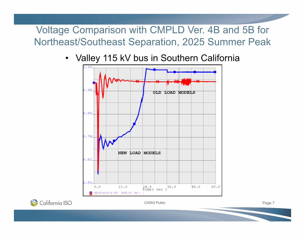
Voltage Comparison with CMPLD Ver. 4B and 5B for Northeast/Southeast Separation, 2025 Summer Peak
• Valley 115 kV bus in Southern California
Page 7

CAISO Public
Frequency Comparison with CMPLD Ver. 4B and 5B for Northeast/Southeast Separation, 2025 Summer Peak
• Valley 115 kV bus in Southern California
Page 8
CAISO Public
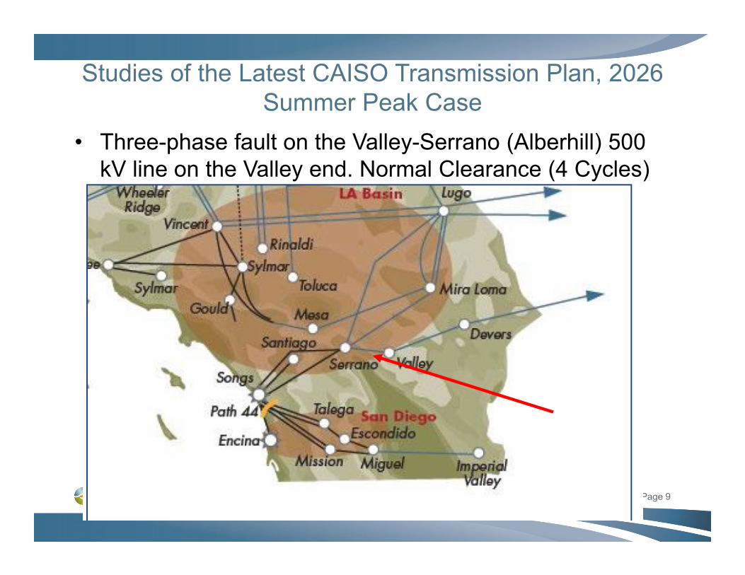
Studies of the Latest CAISO Transmission Plan, 2026 Summer Peak Case
• Three-phase fault on the Valley-Serrano (Alberhill) 500 kV line on the Valley end. Normal Clearance (4 Cycles)
Page 9

CAISO Public
Comparison of the Old and New Composite Load Parameters
• Difference in fractions of different types of motors• Difference in static load coefficients• Update in industrial loads, some new types, new
combinations of motors• For Southern California Internal Mixed feeders
Page 10

CAISO Public
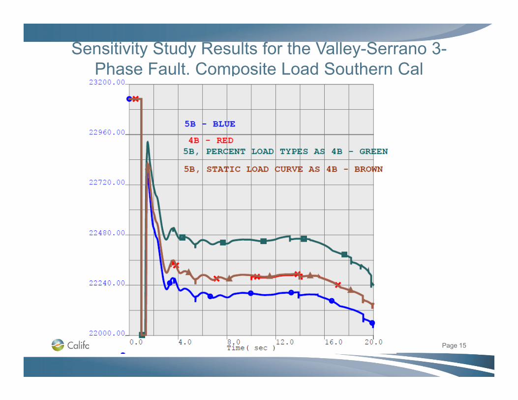
Sensitivity Studies. Cases Studied
1. Composite Load parameters as 5B – latest from WECC2. Composite Load parameters as 4B – before the update3. Composite Load parameters as 5B, but the fraction of
motor types as in 4B4. Composite Load parameters as 5B, but Static Load
coefficients as 4 B
P = Po * (P1c * V P1e + P2c * V P2e + P3 ) * (1 + Pfrq * Δf ) Q = Qo * (Q1c * V Q1e + Q2c * V Q2e + Q3 ) * (1 + Qfrq * Δ f )
Page 11

CAISO Public
Sensitivity Study Results for the Valley-Serrano Three-Phase Fault. Composite Load Loss
Page 12

CAISO Public
Sensitivity Study Results - continued
Page 13

CAISO Public
Sensitivity Study Results for the Valley-Serrano Three-Phase Fault. Composite Load loss Southern Cal
Page 14
CAISO Public
Sensitivity Study Results for the Valley-Serrano 3-Phase Fault. Composite Load Southern Cal
Page 15

CAISO Public
Sensitivity Study Results for the Valley-Serrano 3-Phase Fault. Electronic and Static Load Southern Cal
Page 16
Electronic Load
Static Load

CAISO Public
Sensitivity Study Results for the Valley-Serrano 3-Phase Fault. Motors A and B Southern Cal
Page 17
Motor A
Motor B

CAISO Public
Sensitivity Study Results for the Valley-Serrano 3-Phase Fault. Motors C and D Southern Cal
Page 18
Motor CMotor D

CAISO Public
Another Contingency: Tesla-Metcalf 500 kV 3-Phase Fault at the Tesla End
Most severe in PG&E appeared to be Tesla –Metcalf 500 kV line in San Francisco Bay Area, highest loss of load in PG&E
3-phase fault on the sending end with normal clearance (4 cycles)
Compared Old (4B) and Updated (5B) Parameters
Page 19

CAISO Public
Tesla-Metcalf 3-Phase Fault. Loss of Composite Load in 20 sec, MW
Page 20

CAISO Public
Tesla-Metcalf 3-Phase Fault. Loss of Composite Load in PG&E, MW. System Frequency
Page 21
BLUE – 5B, RED – 4B

CAISO Public
Tesla-Metcalf 3-Phase Fault. Total Composite Load in PG&E, MW.
Page 22
BLUE – 5B, RED – 4B

CAISO Public
Tesla-Metcalf 3-Phase Fault. Electronic and Static Load in PG&E. BLUE – 5B, RED – 4B
Page 23
Electronic Load
Static Load

CAISO Public
Tesla-Metcalf 3-Phase Fault. Motors A and B in PG&E. BLUE – 5B, RED – 4B
Page 24
Motor A
Motor B

CAISO Public
Tesla-Metcalf 3-Phase Fault. Motors C and D in PG&E. BLUE – 5B, RED – 4B
Page 25
Motor C Motor D

CAISO Public
Conclusions and Next Steps• Composite load loss with three-phase faults is a concern, it may
be large and may impact system frequency • The system performance is sensitive to the composite load
parameters, especially for severe contingencies.• It is not clear if performance in actual events will be the same as
in the simulations• The difference in the updated parameters is the fractions of
different types of loads in the composite load model and coefficients of static load. Other updates – industrial loads
• Types of loads that have most impact – single-phase induction motors, motor A and electronic load
• Need more studies to specify parameters of composite load• Next steps – study single-phase faults
Page 26

Public
Implementing, Using, and Validating the Composite Load ModelJuly 27th, 2021 – NERC Load Modeling Working Group

Public
Background Information
Presenter and Company
NERC - Implementing, Using, and Validating the CMLD
- July 27th, 20212

Public
3
Marc Moor
Background on Presenter
• Senior Long-Term Transmission Planning Engineer
• 11 years in industry in transmission planning
• With Evergy (formerly KCP&L) since late 2014
• NERC LMTF/LMWG member since 2015
• Southwest Power Pool – Dynamic Load Task Force member since 2015
• Lead for dynamic studies at Evergy, including composite load model implementation
NERC - Implementing, Using, and Validating the CMLD - July 27th, 2021

Public
4
Evergy
Background on Company
• 2018 Merger between Kansas City Power & Light and Westar Energy
• HQs in Kansas City, MO and Topeka, KS
• Serves 1.6 million customers in Kansas and Missouri
• Member of Southwest Power Pool (SPP)
• Peak Load (summer): ~10 GW
• Approximately 11.5 GW owned generating capacity
• Approximately 4.9 GW of renewable generation in footprint
NERC - Implementing, Using, and Validating the CMLD - July 27th, 2021

Public
5
Evergy - Continued
Background on Company
• PSS®E users (Eastern Interconnection)
• Load Types
• Two fair-sized metropolitan areas: Kansas City and Wichita
• Dense commercial and residential load
• Various large industrial customers
• Fair number of smaller cities with mixture of commercial, residential, rural, and large industrial customers
• Decent amount of rural load: some large customers in remote locations (distant from generation), rural and agricultural loads
NERC - Implementing, Using, and Validating the CMLD - July 27th, 2021

Public
Implementing the Composite Load Model
NERC - Implementing, Using, and Validating the CMLD
- July 27th, 20216
Public
7
Overview
Implementing the Composite Load Model
• Evergy’s Implementation Experience
• Work with Southwest Power Pool/EPRI
• Evergy implementation
• Evergy’s present data-management process
• Implementation Challenges
NERC - Implementing, Using, and Validating the CMLD - July 27th, 2021

Public
8
Overview
Implementing the Composite Load Model
• Evergy’s Implementation Experience
• Work with Southwest Power Pool/EPRI
• Evergy implementation
• Evergy’s present data-management process
• Implementation Challenges
NERC - Implementing, Using, and Validating the CMLD - July 27th, 2021

Public
9
Work with Southwest Power Pool
Implementing the Composite Load Model
• Evergy participates in the SPP Dynamic Load Task Force
• 2016: Survey SPP members and collect data for large, industrial customers in the SPP footprint
• Applied specific industrial load parameterizations as developed by WECC/EPRI (power plant aux, steel mill, paper mill, mine, etc.)
• Created a load parameter collection workbook for use in dynamic case building
• 2017: benchmark large industrial CMLDs
• 2018: implement large industrial CMLDs in region-wide studies
NERC - Implementing, Using, and Validating the CMLD - July 27th, 2021

Public
10
Work with Southwest Power Pool – Continued
Implementing the Composite Load Model
• 2019: begin benchmark and implementation of commercial and residential CMLDs for summer cases only
• SPP members associated all modeled loads with different load types
• Load types were developed by SPP through collaboration with EPRI
• Updated load parameter collection workbook to include different customer classes based on climate zones and parameterization work performed by SPP and EPRI
• 2020: members benchmarked large-scale CMLD implementation
• 2021 and beyond: continue benchmarking and implementation, test the impact of enabling Motor D stalling
NERC - Implementing, Using, and Validating the CMLD - July 27th, 2021

Public
11
Evergy Implementation
Implementing the Composite Load Model
• 2015: test CLOD model
• 2016: abandon CLOD in place of CMLD for large industrials
• 2017-2018: use CMLD for large industrials with some commercial/residential loads (Motor D stalling disabled)
• 2019: associated loads with load types according to NERC Load Model Data Tool (LMDT)
NERC - Implementing, Using, and Validating the CMLD - July 27th, 2021

Public
12
Evergy Implementation
Implementing the Composite Load Model
• 2020: implement CMLD for large non-industrials in TPL studies (Motor D stalling disabled)
• Created an in-house Excel/VBA tool to map LMDT types to SPP/EPRI types used in SPP region
• 2021 and beyond:
• Continue to include CMLD with Motor D stalling disabled for regular work, including annual TPL-001 Planning Assessment
• Perform sensitivity studies with Motor D stalling enabled
• Generator retirement/voltage support studies
• Large customer interconnection studies
NERC - Implementing, Using, and Validating the CMLD - July 27th, 2021

Public
13
Evergy Data Management Process
Implementing the Composite Load Model
• Evergy presently maintains a customized version of the NERC Load Model Data Tool (LMDT)
• Pros:
• Allows Evergy to be in line with NERC expectations
• Allows regional variations of load parameters
• Allows us to maintain consistent load information for both SPP and Evergy studies
• Allows quick and easy ability to create a large number of CMLD records for use in studies
• Cons:
• Load power flow information must be updated manually
• Currently working on import macro
• Parameters for non-summer peak are not easy to sync into the Evergy process; manual configurations must be assigned
• Updates to NERC’s official LMDT must be applied manually to Evergy’s version
NERC - Implementing, Using, and Validating the CMLD - July 27th, 2021

Public
14
Evergy Data Management Process – Continued
Implementing the Composite Load Model
NERC - Implementing, Using, and Validating the CMLD - July 27th, 2021

Public
15
Evergy Data Management Process – Continued
Implementing the Composite Load Model
NERC - Implementing, Using, and Validating the CMLD - July 27th, 2021
• Load Power Flow Mapping

Public
16
Evergy Data Management Process – Continued
Implementing the Composite Load Model
NERC - Implementing, Using, and Validating the CMLD - July 27th, 2021
• Motor Data

Public
17
Evergy Data Management Process – Continued
Implementing the Composite Load Model
NERC - Implementing, Using, and Validating the CMLD - July 27th, 2021
• Load Composition Data

Public
18
Overview
Implementing the Composite Load Model
• “Mechanical” implementation (i.e., what it looks like in software)
• Evergy’s Implementation Experience
• Work with Southwest Power Pool/EPRI
• Evergy implementation
• Evergy’s present data-management process
• Implementation Challenges
NERC - Implementing, Using, and Validating the CMLD - July 27th, 2021

Public
19
Implementation Challenges
Implementing the Composite Load Model
• Increased simulation time: during the 2019 SPP benchmark efforts, Evergy noticed an average run-time increase of about 3 minutes per event
• CMLDs were applied to all ≥ 10MW loads within the SPP footprint
• Original run time was ~5 minutes per event; increased to ~8 minutes per event with the application of all SPP CMLDs
• Results have the potential to differ noticeably from past studies where CMLD was not included
NERC - Implementing, Using, and Validating the CMLD - July 27th, 2021
Public
20
Implementation Challenges (continued)
Implementing the Composite Load Model
• CMLD may have computational issues when applied in tandem with complex load (CLOD) models nearby
• Evergy has experienced PSS®E crashes resulting from CMLD located near (or next to) CLOD models
• NERC default feeder impedances seem to be very high
• Evergy has noticed far-end voltages for power plant auxiliary CMLDs (i.e., the voltage at the far-end bus added by the CMLD) can drop as low as 0.85 p.u.
• Especially for industrials and power plant auxiliaries, Evergy has had to reduce the default R and X feeder values to prevent undue tripping load tripping/stalling (especially power plant auxiliary loads)
NERC - Implementing, Using, and Validating the CMLD - July 27th, 2021

Public
Testing the Composite Load Model
NERC - Implementing, Using, and Validating the CMLD
- July 27th, 202121

Public
22
Comparison Studies – Industrial Only vs. Res/Com/Ind
Testing the Composite Load Model
• Part of SPP benchmarking effort
• TSTALL = disabled
• Impacts were seen mainly for longer lasting, more severe events (e.g., P5)
• Below are images comparing the response of a ~600 MVA coal unit for a P1 versus P5 event at the same location
P1 Event P5 Event
NERC - Implementing, Using, and Validating the CMLD - July 27th, 2021

Public
23
Comparison Studies – Motor D (No Stalling vs. Stalling)
Testing the Composite Load Model
• Motor D stalling can have significant implications
• Evergy has recently started comparing the results of large distributions of the CMLD across Evergy’s footprint with Motor D enabled and disabled (thanks Lafayette!)
• Shown below is a suburban load: same fault, same model, Original (dashed blue) is Motor D stalling disabled, Revised (solid orange) is Motor D stalling enabled (TSTALL = 0.033; voltage at a 161kV bus)
NERC - Implementing, Using, and Validating the CMLD - July 27th, 2021

Public
24
Comparison Studies – Motor D (No Stalling vs. Stalling)
Testing the Composite Load Model
• Shown below is the voltage response at a 161kV bus that feeds a medium-sized (~30 MVA) industrial. The event is a fault at a nearby 161kV bus with normal clearing. “Revised” trace (solid orange) includes Motor D stalling enabled (TSTALL = 0.033)
NERC - Implementing, Using, and Validating the CMLD - July 27th, 2021
Public
25
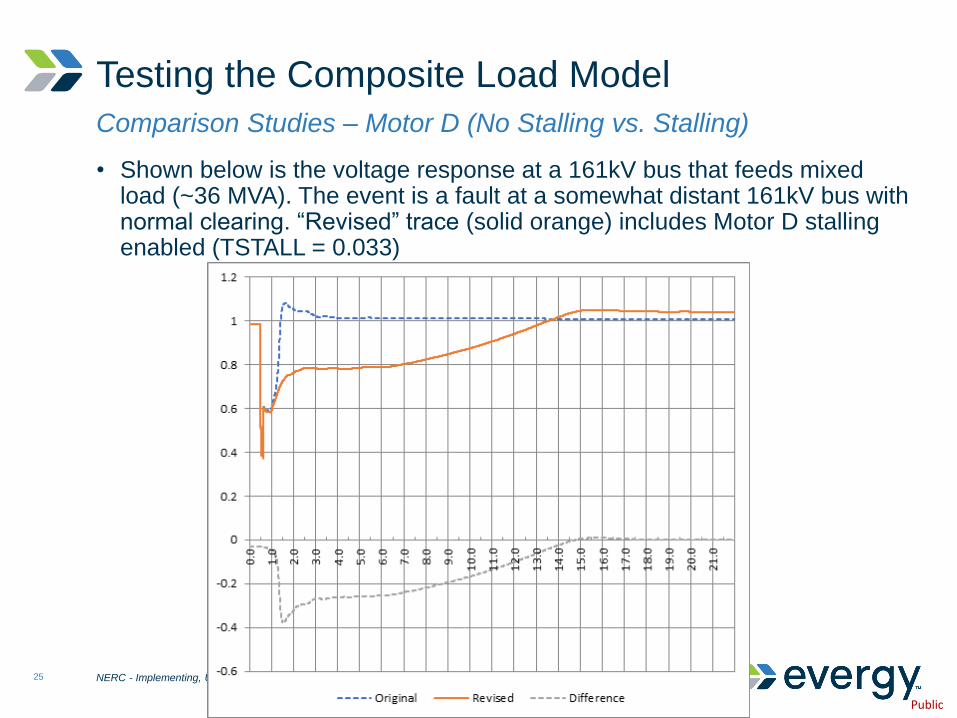
Comparison Studies – Motor D (No Stalling vs. Stalling)
Testing the Composite Load Model
• Shown below is the voltage response at a 161kV bus that feeds mixed load (~36 MVA). The event is a fault at a somewhat distant 161kV bus with normal clearing. “Revised” trace (solid orange) includes Motor D stalling enabled (TSTALL = 0.033)
NERC - Implementing, Using, and Validating the CMLD - July 27th, 2021

Public
26
Event/Field Validation Experience
Testing the Composite Load Model
• Evergy presently has no experience validating the CMLD against actual event data
• For the large, industrial customers Evergy has yet to experience a large disturbance
• For residential and commercial loads, Evergy still needs to develop a validation process
• There is a fair amount of mismatch in Evergy’s legacy footprints for how load information was reported and monitored
• Several internal issues to work out before we can start exploring this front
• Evergy experienced an event in mid-June and collected DFR data from nearby subs
• Possible some validation can be performed
NERC - Implementing, Using, and Validating the CMLD - July 27th, 2021

Public
Questions?
Marc Moor
Senior Transmission Planning Engineer
Evergy, Inc.
O: 816-652-1403

Examination of Composite Load and Variable Frequency Drive Air Conditioning Modeling on FIDVR
Bo Gong - Salt River ProjectAdriana Sullberg, Vijay Vittal – Arizona State University

Introduction
• SRP’s Load Modeling Challenges• High residential A/C load• Past FIDVR event – 2003 Hassayampa event
NERC LMTF 2
~3000MW
~7800MW
SRP

Motivation
• Our Efforts• Understand aggregate load behavior (ongoing)
• Draw some boundary for each type of load behavior
• Modeling/validating bulk system loads (ongoing)• Accurately predict system response (future)• Planning for load response (future)
• SRP/ASU research collaboration on VFD• Under task 1 to “Understand our aggregate load behavior”
• Research project 2019-2020
NERC LMTF 3

Motivation
• Load behavior is evolving
• High A/C electricity usage motivates customers for faster adoption of technologies with better efficiency
• Utilities provide incentive for customer switching to higher efficiency units
• SRP/ASU conduct research to investigate how Variable Frequency Drive (VFD) A/C units being adopted in our footprint
• Understand VFD existing/future impact to FIDVR
NERC LMTF 4

Agenda
Background
Modeling VFD Air Conditioners for Dynamic Studies
Effect of VFD Air Conditioners on FIDVR
A. Cisco Sullberg, M. Wu, V. Vittal, B. Gong and P. Augustin, "Examination of Composite Load and Variable Frequency Drive Air Conditioning Modeling on FIDVR," in IEEE Open Access Journal of Power and Energy, vol. 8, pp. 147-156, 2021, doi: 10.1109/OAJPE.2021.3071692.

Dynamic Load Modeling
• TPL-001-4 Requirement R2.4.1 requires dynamic load modeling
• WECC Composite Load Model -aggregated load model
• Laboratory tests and end-use surveys
• Many parameters are “standard”• Other parameters require feeder-
specific data from the utilityNorth American Electric Reliability Corporation. (2017, Feb.). Reliability Guideline Developing Load Model Composition Data. [Online]. Available: https://www.nerc.com/comm/PC_Reliability_Guidelines_DL/Reliability_Guideline_-_Load_Model_Composition_-_2017-02-28.pdf

• Tested a 2-ton VFD connected air conditioner
• Air conditioner motor tripped for voltage sags greater than 0.75 pu, independent of temperature
• Vc1off can be set to 0.75 pu for dynamic studies of VFD driven air conditioners
• Did not restart for 7 minutes after motor trip
• Phoenix, AZ is more likely to have VFD air conditioners due to the climate
EPRI Technical Update on Load Modeling – Dec 2018
A. Gaikwad, “Technical Update on Load Modeling (3002013562),” Electric Power Research Institute, Palo Alto, CA, 2018.

VFD Usage in Phoenix
• Requested information from Utility Customer Rebate Program
• 17% of rebates in FY20 were for VFD air conditioners

VFD Usage in Phoenix
• Requested information from MagicTouchMechanical in Phoenix, AZ
• Maximum of 30% of installs were VFD, but the number is increasing
• Information from Scottsdale Air Heating and Cooling
• 30% VFD, 40% two-stage, 30% single stage
• Length of time in home
• Size of home
• Package unit upgrade not recommended
“HVAC Packaged Unit vs. Split System: Differences, benefits, and how to choose.,” Petro Home Service. [Online]. Available: https://www.petro.com/resource-center/hvac-packaged-unit-vs-split-system.

VFD Usage Limitations
• Higher cost means a longer time to see a ROI
• There are no VFD-driven packaged
residential ACs
• Conversion to a split system is cost prohibitive
and not recommended
• Smaller homes, homes with limited or no crawl
spaces likely to have a packaged unit
• Packages units under development
“HVAC Packaged Unit vs. Split System: Differences, benefits, and how to choose.,” Petro Home Service. [Online]. Available: https://www.petro.com/resource-center/hvac-packaged-unit-vs-split-system.

• Voltage at motor terminals falls below VStall
for TStall seconds• constant impedance load of RStall+jXStall
• voltage recovers above Vrst for Trst seconds, a fraction of the load, Frst, restarts
• Stalled load linearly trips from temperatures Th1t to Th2t
Single Phase AC Modeling

Modeling VFD Air Conditioners
Given:
• 2025 Heavy Summer Planning Case and Dynamic Data
• Home Age Information
• Number of homes built per year per 69kV feeder xfmr from 1955 to present
• EPRI Technical Update on Load Modeling 2018
• Reciprocating, Scroll, VFD
Study:
• Effect of replacing one- and two- speed residential air conditioners with VFD driven air conditioners

House Age Data
,
,(1)
, , (2)
, , (3)
(4)
(5)
, (6)
The percentage of new air conditioners for a given 69kV bus, ρi, is calculated as:
Where:
The percentage of new air conditioners which are VFD driven for a given 69kV bus, ρVFD,i, can be calculated as:
the total penetration of single-phase motors in
the power system which are VFD driven:, ,
,(7)

House Age Data - Limitations• Assumptions are made in modeling VFD driven air conditioners given the information
available:
I. The 𝛼 parameter is system wide, not bus specific
I. VFD driven air conditioner penetration may lag on feeders where homes are smaller
II. VFD air conditioners are more energy efficient, but 𝑃 was not adjusted in the power flow based on the VFD driven air conditioner penetration
III. The rebate program has limited visibility into consumer behavior
I. Program does not apply to new builds
II. Does not apply to 14 or 15 SEER air conditioners
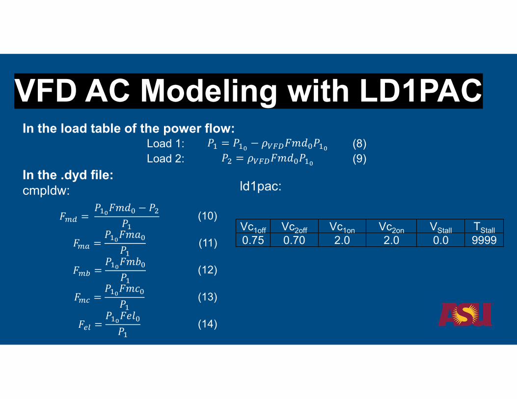
VFD AC Modeling with LD1PACIn the load table of the power flow:
In the .dyd file:cmpldw:
Load 1: (8)Load 2: (9)
𝐹 = 𝑃 𝐹𝑚𝑑 − 𝑃
𝑃(10)
𝐹 =𝑃 𝐹𝑚𝑎
𝑃(11)
𝐹 =𝑃 𝐹𝑚𝑏
𝑃(12)
𝐹 =𝑃 𝐹𝑚𝑐
𝑃(13)
𝐹 =𝑃 𝐹𝑒𝑙
𝑃(14)
Vc1off Vc2off Vc1on Vc2on VStall TStall
0.75 0.70 2.0 2.0 0.0 9999
ld1pac:
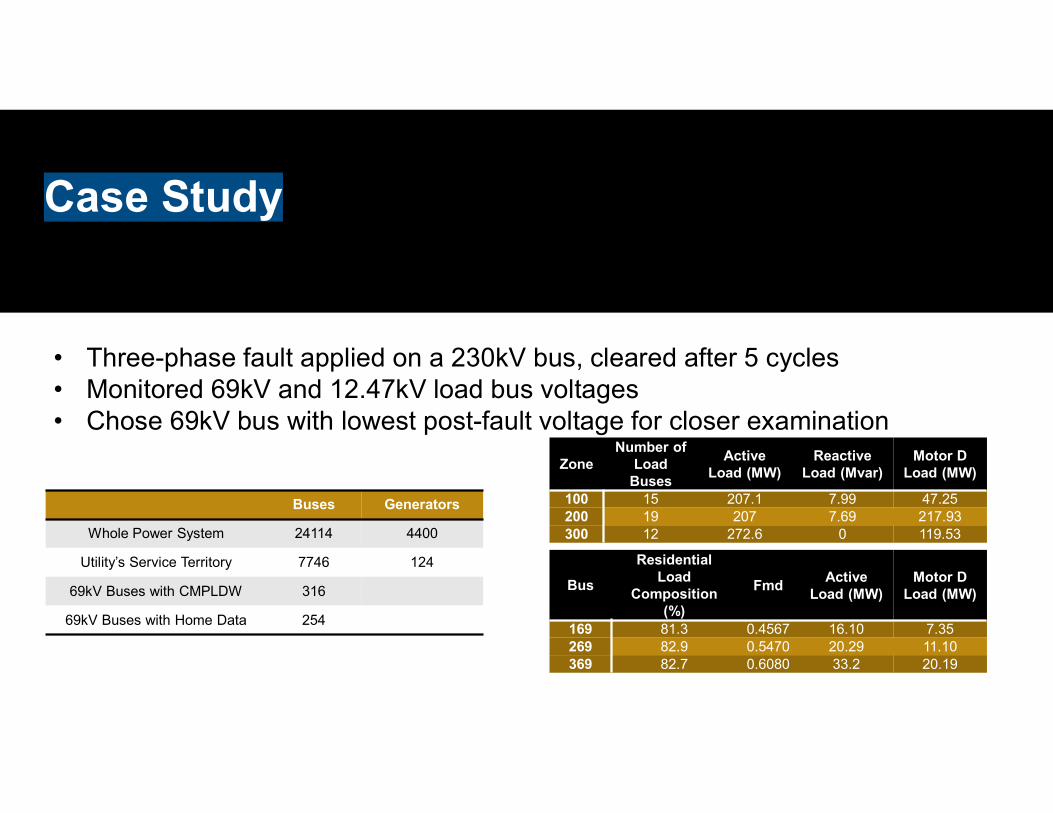
Case Study
ZoneNumber of
Load Buses
Active Load (MW)
Reactive Load (Mvar)
Motor D Load (MW)
100 15 207.1 7.99 47.25200 19 207 7.69 217.93300 12 272.6 0 119.53
Bus
Residential Load
Composition (%)
FmdActive
Load (MW)Motor D
Load (MW)
169 81.3 0.4567 16.10 7.35269 82.9 0.5470 20.29 11.10369 82.7 0.6080 33.2 20.19
• Three-phase fault applied on a 230kV bus, cleared after 5 cycles• Monitored 69kV and 12.47kV load bus voltages• Chose 69kV bus with lowest post-fault voltage for closer examination
Buses Generators
Whole Power System 24114 4400
Utility’s Service Territory 7746 124
69kV Buses with CMPLDW 316
69kV Buses with Home Data 254

Surrounding Bus Voltage following fault on Bus 100. Bus Voltage following fault on Bus 100.
With 0% VFD Air Conditioners Modeled

No single-phase motor (Motor D) stalling output from LD1PAC or CMPLDW.
Best to examine bus active and reactive power to determine motor stalling.
Bus 169 Active and Reactive Power.

Bus 169 Motor A, B, C, and D MW tripped. Cause of Motor D tripping on Bus 169.

VFD Penetration Sensitivity
Based on the VFD replacement definition and modeling methodology defined in an earlier slide, the sensitivity to varying levels of new air conditioners being VFD type is found.
The voltage security is studied at each level of VFD penetration
New ACs which are VFD (%) 5 10 15 20 25 30 50 70 90
Total ACs which are VFD (%) 2.51 5.03 7.54 10.05 12.57 15.08 25.13 35.19 45.24

Bus 112L voltages under varying penetration of VFD driven air conditioners.

Bus 112L Motor D reactive power under varying penetrations of VFD air conditioners.
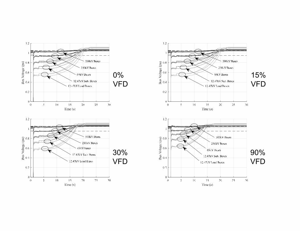
0% VFD
15% VFD
30% VFD
90% VFD

VFD AC Modeling with CMPLDW
No need to change the load representation in the power flow.
In the .dyd file:Adjust change in load representation only:
Adjust for change in power electronic reconnection as a function of added VFD load:
(15)
(16)
(17)

Using only CMPLDW
VFD Penetration at 30%: Bus voltages following fault on Bus 100 using CMPLDW only changing the Fel parameter.
VFD Penetration at 30%: Bus voltages following fault on Bus 100 using CMPLDW changing the Feland Frcel parameters.

Using only CMPLDW
VFD Penetration at 90%: Bus voltages following fault on Bus 100 using CMPLDW only changing the Fel parameter.
VFD Penetration at 90%: Bus voltages following fault on Bus 100 using CMPLDW changing the Feland Frcel parameters.

• Increasing the penetration of VFD driven air condition loadleads to reduced severity of FIDVR events
• The voltage sag following the fault is less severe• The time for the voltage to recover to the pre-fault value is
shortened• Fewer operations of UVLS, resulting in fewer customers being
adversely impacted by the fault• Modeling of VFD driven air conditioners can be simply
achieved, once penetration data is obtained
Conclusions

RELIABILITY | RESILIENCE | SECURITY
Composite Load Model Motor Protection Data StandardizationKannan Sreenivasachar, Olushola Lutalo, Dmitry Kosterev, Parag Mitra, Song Wang, Joe Eto July 27th, 2021

RELIABILITY | RESILIENCE | SECURITY2
• In 2019 and 2020, NERC had requested members to include the Composite Load Model (CMLD) in dynamic simulations and report back to NERC on their performance
• The NERC data sets were sent all members
• Members reported back to NERC over several meetings on the performance of the CMLD model
Background

RELIABILITY | RESILIENCE | SECURITY3
• Phase-1:Motor D Excluded (Motor A trip settings highlighted in red)
Field Test Data
MA MB MC IA IB ICTYPE M3 M3 M3 M3 M3 M3LF 0.75 0.75 0.75 0.8 0.8 0.8Ra 0.02 0.02 0.02 0.01 0.005 0.01Ls 1.8 1.8 1.8 3.1 4 3.1Lps 0.12 0.19 0.19 0.1384 0.185 0.185Lpps 0.104 0.14 0.14 0.121 0.16 0.16Tpo 0.08 0.2 0.2 0.1028 0.8 0.35Tppo 0.0021 0.0026 0.0026 0.0028 0.0044 0.0036H 0.1 0.5 0.1 0.1 0.5 0.15Etrq 0 2 2 0 2 2Vtr1 0.5 0 0 0.7 0.7 0.7Ttr1 0.5 9999 9999 0.05 0.05 0.05Ftr1 0.33 0 0 0.3 0.3 0.3Vrc1 1 1 1 1 1 1Trc1 9999 9999 9999 9999 9999 9999Vtr2 0.55 0 0 0.6 0.6 0.6Ttr2 1 9999 9999 0.02 0.02 0.02Ftr2 0.33 0 0 0.7 0.5 0.5Vrc2 1 1 1 1 0.75 0.75Trc2 9999 9999 9999 99999 0.25 0.25
RELIABILITY | RESILIENCE | SECURITY4
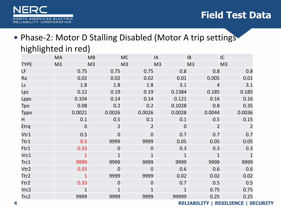
• Phase-2: Motor D Stalling Disabled (Motor A trip settings highlighted in red)
Field Test Data
MA MB MC IA IB ICTYPE M3 M3 M3 M3 M3 M3LF 0.75 0.75 0.75 0.8 0.8 0.8Ra 0.02 0.02 0.02 0.01 0.005 0.01Ls 1.8 1.8 1.8 3.1 4 3.1Lps 0.12 0.19 0.19 0.1384 0.185 0.185Lpps 0.104 0.14 0.14 0.121 0.16 0.16Tpo 0.08 0.2 0.2 0.1028 0.8 0.35Tppo 0.0021 0.0026 0.0026 0.0028 0.0044 0.0036H 0.1 0.5 0.1 0.1 0.5 0.15Etrq 0 2 2 0 2 2Vtr1 0.5 0 0 0.7 0.7 0.7Ttr1 0.5 9999 9999 0.05 0.05 0.05Ftr1 0.33 0 0 0.3 0.3 0.3Vrc1 1 1 1 1 1 1Trc1 9999 9999 9999 9999 9999 9999Vtr2 0.55 0 0 0.6 0.6 0.6Ttr2 1 9999 9999 0.02 0.02 0.02Ftr2 0.33 0 0 0.7 0.5 0.5Vrc2 1 1 1 1 0.75 0.75Trc2 9999 9999 9999 99999 0.25 0.25
RELIABILITY | RESILIENCE | SECURITY5
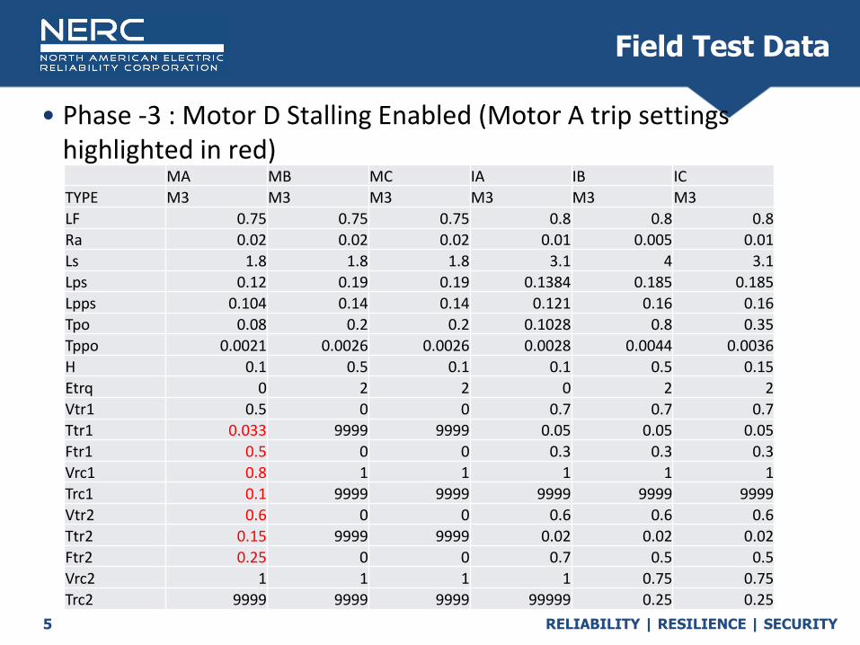
• Phase -3 : Motor D Stalling Enabled (Motor A trip settings highlighted in red)
Field Test Data
MA MB MC IA IB ICTYPE M3 M3 M3 M3 M3 M3LF 0.75 0.75 0.75 0.8 0.8 0.8Ra 0.02 0.02 0.02 0.01 0.005 0.01Ls 1.8 1.8 1.8 3.1 4 3.1Lps 0.12 0.19 0.19 0.1384 0.185 0.185Lpps 0.104 0.14 0.14 0.121 0.16 0.16Tpo 0.08 0.2 0.2 0.1028 0.8 0.35Tppo 0.0021 0.0026 0.0026 0.0028 0.0044 0.0036H 0.1 0.5 0.1 0.1 0.5 0.15Etrq 0 2 2 0 2 2Vtr1 0.5 0 0 0.7 0.7 0.7Ttr1 0.033 9999 9999 0.05 0.05 0.05Ftr1 0.5 0 0 0.3 0.3 0.3Vrc1 0.8 1 1 1 1 1Trc1 0.1 9999 9999 9999 9999 9999Vtr2 0.6 0 0 0.6 0.6 0.6Ttr2 0.15 9999 9999 0.02 0.02 0.02Ftr2 0.25 0 0 0.7 0.5 0.5Vrc2 1 1 1 1 0.75 0.75Trc2 9999 9999 9999 99999 0.25 0.25

RELIABILITY | RESILIENCE | SECURITY6
• Comparison of Motor A data between Phase -1, 2 and 3 for RES,COM,MIX and RAG (red indicates differences)
Field Test Data
Phase-1 MA Phase -2 MA Phase-3 MATYPE M3 M3 M3
LF 0.75 0.75 0.75Ra 0.02 0.02 0.02Ls 1.8 1.8 1.8
Lps 0.12 0.12 0.12Lpps 0.104 0.104 0.104Tpo 0.08 0.08 0.08
Tppo 0.0021 0.0021 0.0021H 0.1 0.1 0.1
Etrq 0 0 0Vtr1 0.5 0.5 0.5Ttr1 0.5 0.5 0.033Ftr1 0.33 0.33 0.5Vrc1 1 1 0.8Trc1 9999 9999 0.1Vtr2 0.55 0.55 0.6Ttr2 1 1 0.15Ftr2 0.33 0.33 0.25Vrc2 1 1 1Trc2 9999 9999 9999

RELIABILITY | RESILIENCE | SECURITY7
• Phase -1 and Phase -2 data for Motor A are not the same as the Phase-3 Motor A settings in the Field Test Data.
• Based on the presentations made at the NERC LMTF meetings, it has been decided to standardize the voltage and trip settings among the different phases of the CMLD Load Model Consistency in the data among all phases of the model Ease of maintaining one set of data for Motors A, B and C for Residential,
Commercial, MIX, and RAG Data for Motor A, B and C for Industrial Motors are already consistent Only variation would be in the application of Motor D
Standardization

RELIABILITY | RESILIENCE | SECURITY8
• Standardization of Motor A, B and C data for RES,COM,MIX, and RAG
Standardization
MA MB MC IA IB ICTYPE M3 M3 M3 M3 M3 M3LF 0.75 0.75 0.75 0.8 0.8 0.8Ra 0.02 0.02 0.02 0.01 0.005 0.01Ls 1.8 1.8 1.8 3.1 4 3.1Lps 0.12 0.19 0.19 0.1384 0.185 0.185Lpps 0.104 0.14 0.14 0.121 0.16 0.16Tpo 0.08 0.2 0.2 0.1028 0.8 0.35Tppo 0.0021 0.0026 0.0026 0.0028 0.0044 0.0036H 0.1 0.5 0.1 0.1 0.5 0.15Etrq 0 2 2 0 2 2Vtr1 0.5 0 0 0.7 0.7 0.7Ttr1 0.033 9999 9999 0.05 0.05 0.05Ftr1 0.5 0 0 0.3 0.3 0.3Vrc1 0.8 1 1 1 1 1Trc1 0.1 9999 9999 9999 9999 9999Vtr2 0.6 0 0 0.6 0.6 0.6Ttr2 0.15 9999 9999 0.02 0.02 0.02Ftr2 0.25 0 0 0.7 0.5 0.5Vrc2 1 1 1 1 0.75 0.75Trc2 9999 9999 9999 99999 0.25 0.25

RELIABILITY | RESILIENCE | SECURITY9
• Motor D data
Standardization
ACTYPE Default Low HighLFm 1
CompPF 0.98Vstall 0.45 0.4 0.45Rstall 0.1Xstall 0.1Tstall* 0.033/-1/999
Frst 0.2 0.2 0.6Vrst 0.95Trst 0.3Fuvr 0.1 0 0.5Vtr1 0.6Ttr1 0.02Vtr2 0Ttr2 9999
Vc1off 0.5Vc2off 0.4VC1on 0.6 0.6 0.75VC2on 0.5 0.5 0.65
ACTYPE Default Low HighTth 10 5 15
Th1t 0.7Th2t 1.9
Tv 0.025Tf 0.05
LFadj 0Kp1 0Np1 1Kq1 6Nq1 2Kp2 12Np2 3.2Kq2 11Nq2 2.5Vbrk 0.86
CmpKpf 1CmpKqf -3.3
Notes:1. Delayed reconnection (high values of VC1on and VC2on) are recommended for use while studying extreme events2. Tth affects simulations in conjunction with Th1t and Th2t. It is recommended that Tth is adjusted as needed while keeping
Th1t and Th2t fixed3. If more than expected motor D trips, FRST needs to be increased towards the higher end.
*• Tstall = 0.033 stalling
enabled• Tstall = -1 stalling enabled
via Vstall-Tstall curve• Tstall = 999 stalling
disabled

RELIABILITY | RESILIENCE | SECURITY10
Standardization
• Some useful references for trip settings1. https://pserc.wisc.edu/wp-
content/uploads/sites/755/2018/08/T-16_Final-Report_Oct-2005.pdf [pserc.wisc.edu]
2. https://certs.lbl.gov/publications/commercial-building-motor-protection
3. https://eta-publications.lbl.gov/sites/default/files/robles-commercial-3-phase-rooftop-airconditioner-report.pdf
General repository of FIDVR related papers/documents (CourtseyJoe Eto LBNL)1. https://certs.lbl.gov/initiatives/fidvr

RELIABILITY | RESILIENCE | SECURITY11