1

M.I.E.T. ENGINEERING COLLEGE

(Approved by AICTE and Affiliated to Anna University Chennai)

TRICHY – PUDUKKOTTAI ROAD, TIRUCHIRAPPALLI – 620 007

DEPARTMENT OF ELECTRICAL AND

ELECTRONICS ENGINEERING

COURSE MATERIAL

EE6601 SOLID STATE DRIVES

III YEAR - VI SEMESTER

2

EE6601 SOLID STATE DRIVES . UNIT I DRIVE CHARACTERISTICS 9 Electric drive – Equations governing motor load dynamics – steady state stability – multi quadrant Dynamics: acceleration, deceleration, starting & stopping – typical load torque characteristics – Selection of motor. UNIT II CONVERTER / CHOPPER FED DC MOTOR DRIVE 9 Steady state analysis of the single and three phase converter fed separately excited DC motor Drive–continuous and discontinuous conduction– Time ratio and current limit control – 4 quadrant operations of converter / chopper fed drive. UNIT III INDUCTION MOTOR DRIVES 9 Stator voltage control–energy efficient drive–v/f control–constant air-gap flux–field weakening mode – voltage / current fed inverter – closed loop control. UNIT IV SYNCHRONOUS MOTOR DRIVES 9 V/f control and self control of synchronous motor: Margin angle control and power factor control –permanent magnet synchronous motor. UNIT V DESIGN OF CONTROLLERS FOR DRIVES 9 Transfer function for DC motor / load and converter – closed loop control with Current and speed feedback–armature voltage control and field weakening mode – Design of controllers; current controller and speed controller- converter selection and characteristics.

TOTAL: 45 PERIODS OUTCOMES:

Ability to understand and apply basic science, circuit theory, Electro-magnetic field theory control theory and apply them to electrical engineering problems. TEXT BOOKS: 1. Gopal K.Dubey, Fundamentals of Electrical Drives, Narosa Publishing House, 1992. 2. Bimal K.Bose. Modern Power Electronics and AC Drives, Pearson Education, 2002. 3. R.Krishnan, Electric Motor & Drives: Modeling, Analysis and Control, Prentice Hall of India, 2001. REFERENCES: 1. John Hindmarsh and Alasdain Renfrew, “Electrical Machines and Drives System,” Elsevier 2012. 2. Shaahin Felizadeh, “Electric Machines and Drives”, CRC Press(Taylor and Francis Group),2013. 3. S.K.Pillai, A First course on Electrical Drives, Wiley Eastern Limited, 1993. 4. S. Sivanagaraju, M. Balasubba Reddy, A. Mallikarjuna Prasad “Power semiconductor drives”PHI, 5th printing, 2013. 5. N.K.De., P.K.SEN”Electric drives” PHI, 2012. 6. Vedam Subramanyam, ”Thyristor Control of Electric Drives”, Tata McGraw Hill, 2007.

3

UNIT-I

DRIVE CHARACTERISTICS 1.1. Electrical Drives:

Motion control is required in large number of industrial and domestic applications

like transportation systems, rolling mills, paper machines, textile mills, machine tools, fans,

pumps, robots, washing machines etc. Systems employed for motion control are called

DRIVES, and may employ any of prime movers such as diesel or petrol engines, gas or

steam turbines, steam engines, hydraulic motors and electric motors, for supplying

mechanical energy for motion control. Drives employing electric motors are known as

Electrical Drives.

An Electric Drive can be defined as an electromechanical device for converting

electrical energy into mechanical energy to impart motion to different machines and

mechanisms for various kinds of process control.

1.1.1. Classification of Electric Drives

1.1.1.1 According to Mode of Operation

Continuous duty drives Short time duty drives Intermittent duty drives

1.1.1.2. According to Means of Control

Manual Semi-automatic Automatic

1.1.1.3. According to Number of machines

Individual drive Group drive Multi-motor drive

1.1.1.4. According to Dynamics and Transients

Uncontrolled transient period Controlled transient period

1.1.1.5. According to Methods of Speed Control

Reversible and non-reversible uncontrolled constant speed. Reversible and non-reversible step speed control. Variable position control.

4

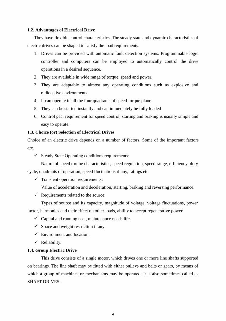
1.2. Advantages of Electrical Drive

They have flexible control characteristics. The steady state and dynamic characteristics of

electric drives can be shaped to satisfy the load requirements.

1. Drives can be provided with automatic fault detection systems. Programmable logic

controller and computers can be employed to automatically control the drive

operations in a desired sequence.

2. They are available in wide range of torque, speed and power.

3. They are adaptable to almost any operating conditions such as explosive and

radioactive environments

4. It can operate in all the four quadrants of speed-torque plane

5. They can be started instantly and can immediately be fully loaded

6. Control gear requirement for speed control, starting and braking is usually simple and

easy to operate.

1.3. Choice (or) Selection of Electrical Drives

Choice of an electric drive depends on a number of factors. Some of the important factors

are.

Steady State Operating conditions requirements:Nature of speed torque characteristics, speed regulation, speed range, efficiency, duty

cycle, quadrants of operation, speed fluctuations if any, ratings etc

Transient operation requirements:Value of acceleration and deceleration, starting, braking and reversing performance.

Requirements related to the source:Types of source and its capacity, magnitude of voltage, voltage fluctuations, power

factor, harmonics and their effect on other loads, ability to accept regenerative power

Capital and running cost, maintenance needs life. Space and weight restriction if any. Environment and location. Reliability.

1.4. Group Electric Drive

This drive consists of a single motor, which drives one or more line shafts supported

on bearings. The line shaft may be fitted with either pulleys and belts or gears, by means of

which a group of machines or mechanisms may be operated. It is also sometimes called as

SHAFT DRIVES.

5

Advantages

A single large motor can be used instead of number of small motors

Disadvantages

There is no flexibility. If the single motor used develops fault, the whole process will be

stopped.

1.4.1. Individual Electric Drive

In this drive each individual machine is driven by a separate motor. This motor also

imparts motion to various parts of the machine.

1.4.2. Multi Motor Electric Drive

In this drive system, there are several drives, each of which serves to actuate one of the

working parts of the drive mechanisms. E.g.,

Complicated metal cutting machine tools

Paper making industries, rolling machines etc.

1.5. Classification of Electrical Drives

Another main classification of electric drive is

DC drive AC drive

1.5.1. Applications

Paper mills Cement Mills Textile mills Sugar Mills Steel Mills Electric Traction Petrochemical Industries Electrical Vehicles

1.6. Dynamics of Motor Load System

1.6.1. Principle of operation

A motor generally drives a load (Machines) through some transmission system. While

motor always rotates, the load may rotate or undergo a translational motion.

Load speed may be different from that of motor, and if the load has many parts, their

speed may be different and while some parts rotate others may go through a translational

motion.

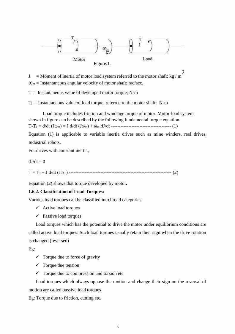
Equivalent rotational system of motor and load is shown in the figure.1.

6

Figure.1.

J = Moment of inertia of motor load system referred to the motor shaft; kg / m2

ωm = Instantaneous angular velocity of motor shaft; rad/sec. T = Instantaneous value of developed motor torque; N-m Tl = Instantaneous value of load torque, referred to the motor shaft; N-m

Load torque includes friction and wind age torque of motor. Motor-load system shown in figure can be described by the following fundamental torque equation. T-T1 = d/dt (Jωm) = J d/dt (Jωm) + ωm dJ/dt -------------------------------------- (1)

Equation (1) is applicable to variable inertia drives such as mine winders, reel drives,

Industrial robots. For drives with constant inertia,

dJ/dt = 0

T = T1 + J d/dt (Jωm) ----------------------------------------------------------------- (2)

Equation (2) shows that torque developed by motor.

1.6.2. Classification of Load Torques:

Various load torques can be classified into broad categories.

Active load torques Passive load torquesLoad torques which has the potential to drive the motor under equilibrium conditions are

called active load torques. Such load torques usually retain their sign when the drive rotation

is changed (reversed)

Eg:

Torque due to force of gravity Torque due tension Torque due to compression and torsion etcLoad torques which always oppose the motion and change their sign on the reversal of

motion are called passive load torques

Eg: Torque due to friction, cutting etc.

7

1.6.3. Components of Load Torques:

The load torque Tl can be further divided into following components

Friction Torque (TF):Friction will be present at the motor shaft and also in various parts of the load. TF is the

equivalent value of various friction torques referred to the motor shaft.

Windage Torque (TW)When motor runs, wind generates a torque opposing the motion. This is known as

windage torque.

Torque required to do useful mechanical workNature of this torque depends upon particular application. It may be constant and

independent of speed.

It may be some function of speed, it may be time invariant or time variant, its nature may

also change with the load’s mode of operation.

Friction at zero speed is called diction or static friction. In order to start the drive the

motor should at least exceeds diction. Friction torque can also be resolved into three

components

Component Tv varies linearly with speed is called VISCOUS friction and is given by

Tv = B ωm Where, B is viscous friction co-efficient.

Another component TC, which is independent of speed, is known as COULOMB

friction. Third component Ts accounts for additional torque present at stand still. Since Ts is

present only at stand still it is not taken into account in the dynamic analysis. Wind age

torque, TW which is proportional to speed Squared is given by,

Tw = C ωm2

From the above discussions, for finite speed T1 = TL + B ωm + TC + C ωm

2

1.7. Characteristics of Different types of Loads

One of the essential requirements in the section of a particular type of motor for

driving a machine is the matching of speed-torque characteristics of the given drive unit and

that of the motor. Therefore the knowledge of how the load torque varies with speed of the

driven machine is necessary. Different types of loads exhibit different speed torque

characteristics. However, most of the industrial loads can be classified into the following four

categories.

8

1.7.1. Constant torque type load

Torque proportional to speed (Generator Type load) Torque proportional to square of the speed (Fan type load) Torque inversely proportional to speed (Constant power type load)

1.7.2. Constant Torque characteristics:

Most of the working machines that have mechanical nature of work like shaping,

cutting, grinding or shearing, require constant torque irrespective of speed. Similarly cranes

during the hoisting and conveyors handling constant weight of material per unit time also

exhibit this type of Characteristics.

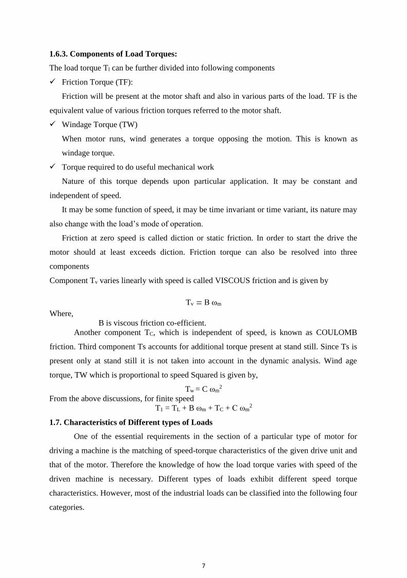
1.7.3. Torque Proportional to speed:

Separately excited dc generators connected to a constant resistance load, eddy current brakes have speed torque characteristics given by

T=k

Figure.21.7.4. Torque proportional to square of the speed:

Another type of load met in practice is the one in which load torque is proportional to

the square of the speed.

Examples:

Fans rotary pumps,

9

Compressors Ship propellers

Figure.3.

1.7.5. Torque Inversely proportional to speed:

Certain types of lathes, boring machines, milling machines, steel mill coiler and electric traction load exhibit hyperbolic speed-torque characteristics

Figure.4 1.8. Multi quadrant Operation:

1.8.1. Different modes of operation

For consideration of multi quadrant operation of drives, it is useful to establish

suitable conventions about the signs of torque and speed.

10

A motor operates in two modes – Motoring and braking. In motoring, it converts

electrical energy into mechanical energy, which supports its motion .In braking it works as a

generator converting mechanical energy into electrical energy and thus opposes the motion.

Now consider equilibrium point B which is obtained when the same motor drives

another load as shown in the figure. A decrease in speed causes the load torque to become

greater than the motor torque, electric drive decelerates and operating point moves away

from point B.

Similarly when working at point B and increase in speed will make motor torque

greater than the load torque, which will move the operating point away from point B

Similarly operation in quadrant III and IV can be identified as reverse motoring and

reverse braking since speed in these quadrants is negative.

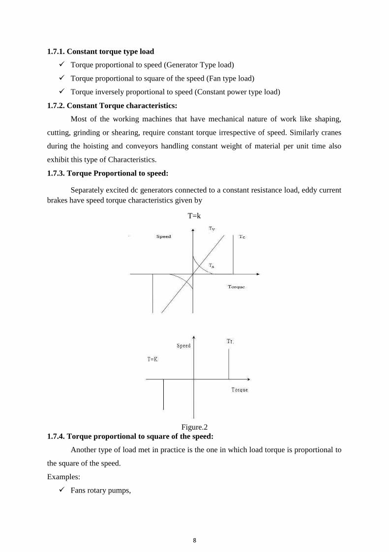
For better understanding of the above notations, let us consider operation of hoist in

four quadrants as shown in the figure. Direction of motor and load torques and direction of

speed are marked by arrows

The figure at the right represents a DC motor attached to an inertial load. Motor can

provide motoring and braking operations for both forward and reverse directions.

Figure shows the torque and speed co-ordinates for both forward and reverse motions.

Power developed by a motor is given by the product of speed and torque. For motoring

operations Power developed is positive and for braking operations power developed is

negative.

For better understanding of the above notations, let us consider operation of hoist in

four quadrants as shown in the figure. Direction of motor and load torques and direction of

speed are marked by arrows.

Figure.5

11

Figure.6.

A hoist consists of a rope wound on a drum coupled to the motor shaft one end of the

rope is tied to a cage which is used to transport man or material from one level to another

level . Other end of the rope has a counter weight. Weight of the counter weight is chosen to

be higher than the weight of empty cage but lower than of a fully loaded cage.

Forward direction of motor speed will be one which gives upward motion of the

cage. Load torque line in quadrants I and IV represents speed-torque characteristics of the

loaded hoist. This torque is the difference of torques due to loaded hoist and counter weight.

The load torque in quadrants II and III is the speed torque characteristics for an empty hoist.

12

This torque is the difference of torques due to counter weight and the empty hoist. Its

sigh is negative because the counter weight is always higher than that of an empty cage. The

quadrant I operation of a hoist requires movement of cage upward, which corresponds to the

positive motor speed which is in counter clockwise direction here. This motion will be

obtained if the motor products positive torque in CCW direction equal to the magnitude of

load torque TL1.

Since developed power is positive, this is forward motoring operation. Quadrant IV is

obtained when a loaded cage is lowered. Since the weight of the loaded cage is higher than that

of the counter weight. It is able to overcome due to gravity itself. In order to limit the cage

within a safe value, motor must produce a positive torque T equal to TL2 in anticlockwise

direction. As both power and speed are negative, drive is operating in reverse braking

operation. Operation in quadrant II is obtained when an empty cage is moved up. Since a

counter weigh is heavier than an empty cage, it’s able to pull it up.

In order to limit the speed within a safe value, motor must produce a braking torque

equal to TL2 in clockwise direction. Since speed is positive and developed power is negative,

it’s forward braking operation.

Operation in quadrant III is obtained when an empty cage is lowered. Since an empty

cage has a lesser weight than a counter weight, the motor should produce a torque in CW

direction. Since speed is negative and developed power is positive, this is reverse motoring

operation. During transient condition, electrical motor can be assumed to be in electrical

equilibrium implying that steady state speed torque curves are also applicable to the transient

state operation.

1.9. Steady State Stability:

1.9.1. Speed-Torque characteristics

Equilibrium speed of motor-load system can be obtained when motor torque equals

the load torque. Electric drive system will operate in steady state at this speed, provided it is

the speed of stable state equilibrium.

Concept of steady state stability has been developed to readily evaluate the stability

of an equilibrium point from the steady state speed torque curves of the motor and load

system. In most of the electrical drives, the electrical time constant of the motor is negligible

compared with the mechanical time constant. During transient condition, electrical motor can

be assumed to be in electrical equilibrium implying that steady state speed torque curves are

also applicable to the transient state operation.

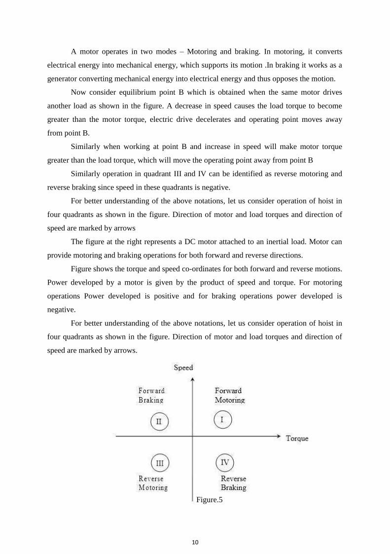
Now, consider the steady state equilibrium point A shown in figure.7 below.

13

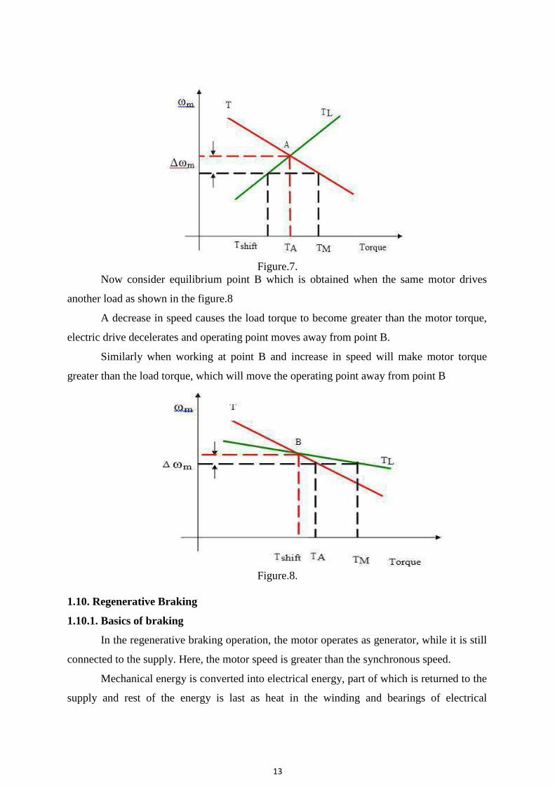
Figure.7. Now consider equilibrium point B which is obtained when the same motor drives

another load as shown in the figure.8

A decrease in speed causes the load torque to become greater than the motor torque,

electric drive decelerates and operating point moves away from point B.

Similarly when working at point B and increase in speed will make motor torque

greater than the load torque, which will move the operating point away from point B

Figure.8. 1.10. Regenerative Braking

1.10.1. Basics of braking

In the regenerative braking operation, the motor operates as generator, while it is still

connected to the supply. Here, the motor speed is greater than the synchronous speed.

Mechanical energy is converted into electrical energy, part of which is returned to the

supply and rest of the energy is last as heat in the winding and bearings of electrical

14

machines pass smoothly from motoring region to generating region, when over driven by the

load.

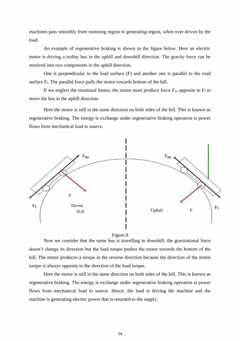
An example of regenerative braking is shown in the figure below. Here an electric

motor is driving a trolley bus in the uphill and downhill direction. The gravity force can be

resolved into two components in the uphill direction.

One is perpendicular to the load surface (F) and another one is parallel to the road

surface Fl. The parallel force pulls the motor towards bottom of the hill.

If we neglect the rotational losses, the motor must produce force Fm opposite to Fl to

move the bus in the uphill direction.

Here the motor is still in the same direction on both sides of the hill. This is known as

regenerative braking. The energy is exchange under regenerative braking operation is power

flows from mechanical load to source.

Figure.9 Now we consider that the same bus is travelling in downhill, the gravitational force

doesn’t change its direction but the load torque pushes the motor towards the bottom of the

hill. The motor produces a torque in the reverse direction because the direction of the motor

torque is always opposite to the direction of the load torque.

Here the motor is still in the same direction on both sides of the hill. This is known as

regenerative braking. The energy is exchange under regenerative braking operation is power

flows from mechanical load to source. Hence, the load is driving the machine and the

machine is generating electric power that is returned to the supply.

15

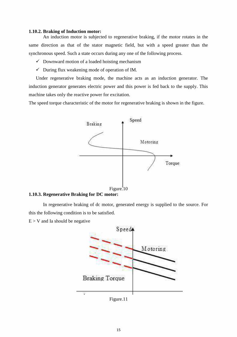
1.10.2. Braking of Induction motor: An induction motor is subjected to regenerative braking, if the motor rotates in the

same direction as that of the stator magnetic field, but with a speed greater than the

synchronous speed. Such a state occurs during any one of the following process.

Downward motion of a loaded hoisting mechanism During flux weakening mode of operation of IM.Under regenerative braking mode, the machine acts as an induction generator. The

induction generator generates electric power and this power is fed back to the supply. This

machine takes only the reactive power for excitation.

The speed torque characteristic of the motor for regenerative braking is shown in the figure.

Figure.10 1.10.3. Regenerative Braking for DC motor:

In regenerative braking of dc motor, generated energy is supplied to the source. For

this the following condition is to be satisfied.

E > V and Ia should be negative

Figure.11

16

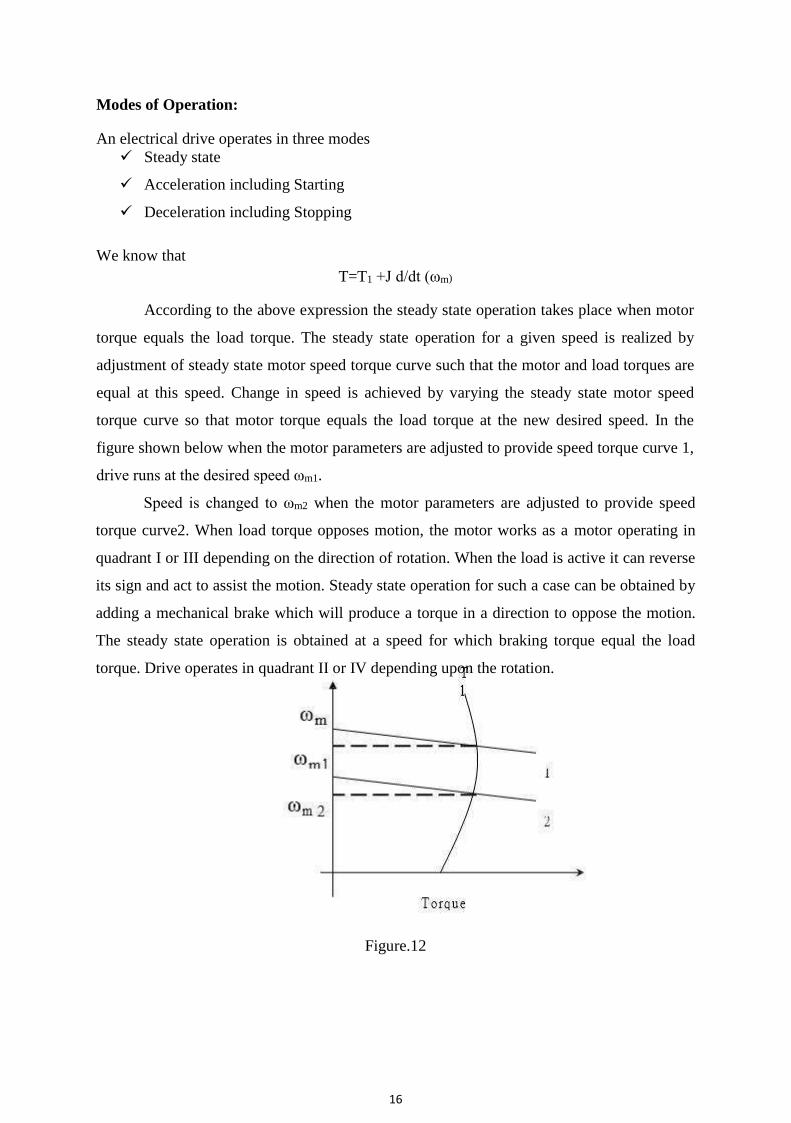
Modes of Operation: An electrical drive operates in three modes Steady state Acceleration including Starting Deceleration including Stopping

We know that

T=T1 +J d/dt (ωm)

According to the above expression the steady state operation takes place when motor

torque equals the load torque. The steady state operation for a given speed is realized by

adjustment of steady state motor speed torque curve such that the motor and load torques are

equal at this speed. Change in speed is achieved by varying the steady state motor speed

torque curve so that motor torque equals the load torque at the new desired speed. In the

figure shown below when the motor parameters are adjusted to provide speed torque curve 1,

drive runs at the desired speed ωm1.

Speed is changed to ωm2 when the motor parameters are adjusted to provide speed

torque curve2. When load torque opposes motion, the motor works as a motor operating in

quadrant I or III depending on the direction of rotation. When the load is active it can reverse

its sign and act to assist the motion. Steady state operation for such a case can be obtained by

adding a mechanical brake which will produce a torque in a direction to oppose the motion.

The steady state operation is obtained at a speed for which braking torque equal the load

torque. Drive operates in quadrant II or IV depending upon the rotation.

Figure.12

17

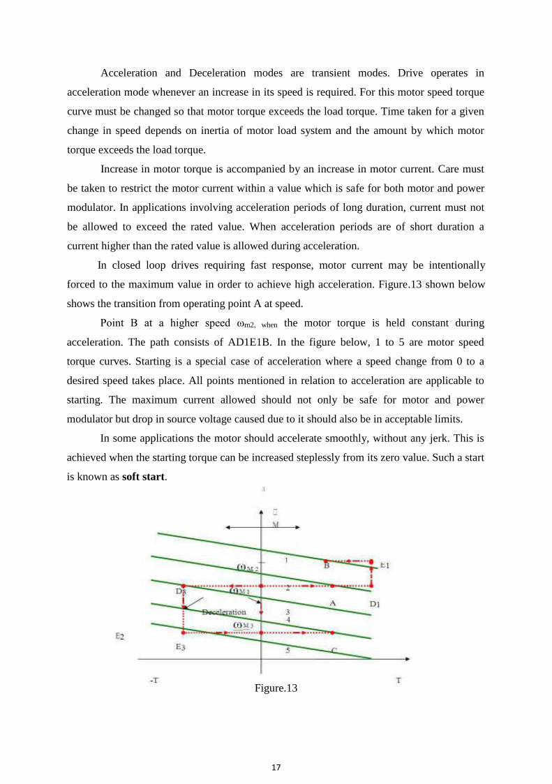
Acceleration and Deceleration modes are transient modes. Drive operates in

acceleration mode whenever an increase in its speed is required. For this motor speed torque

curve must be changed so that motor torque exceeds the load torque. Time taken for a given

change in speed depends on inertia of motor load system and the amount by which motor

torque exceeds the load torque.

Increase in motor torque is accompanied by an increase in motor current. Care must

be taken to restrict the motor current within a value which is safe for both motor and power

modulator. In applications involving acceleration periods of long duration, current must not

be allowed to exceed the rated value. When acceleration periods are of short duration a

current higher than the rated value is allowed during acceleration.

In closed loop drives requiring fast response, motor current may be intentionally

forced to the maximum value in order to achieve high acceleration. Figure.13 shown below

shows the transition from operating point A at speed.

Point B at a higher speed ωm2, when the motor torque is held constant during

acceleration. The path consists of AD1E1B. In the figure below, 1 to 5 are motor speed

torque curves. Starting is a special case of acceleration where a speed change from 0 to a

desired speed takes place. All points mentioned in relation to acceleration are applicable to

starting. The maximum current allowed should not only be safe for motor and power

modulator but drop in source voltage caused due to it should also be in acceptable limits.

In some applications the motor should accelerate smoothly, without any jerk. This is

achieved when the starting torque can be increased steplessly from its zero value. Such a start

is known as soft start.

Figure.13

18

UNIT II

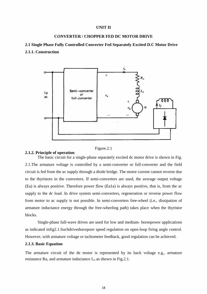
CONVERTER / CHOPPER FED DC MOTOR DRIVE 2.1 Single Phase Fully Controlled Converter Fed Separately Excited D.C Motor Drive

2.1.1. Construction

Figure.2.1 2.1.2. Principle of operation

The basic circuit for a single-phase separately excited dc motor drive is shown in Fig.

2.1.The armature voltage is controlled by a semi-converter or full-converter and the field

circuit is fed from the ac supply through a diode bridge. The motor current cannot reverse due

to the thyristors in the converters. If semi-converters are used, the average output voltage

(Ea) is always positive. Therefore power flow (Ea1a) is always positive, that is, from the ac

supply to the dc load. In drive system semi-converters, regeneration or reverse power flow

from motor to ac supply is not possible. In semi-converters free-wheel (i.e., dissipation of

armature inductance energy through the free-wheeling path) takes place when the thyristor

blocks.

Single-phase full-wave drives are used for low and medium- horsepower applications

as indicated infig2.1.Suchdriveshavepoor speed regulation on open-loop firing angle control.

However, with armature voltage or tachometer feedback, good regulation can be achieved.

2.1.3. Basic Equation The armature circuit of the de motor is represented by its back voltage e.g., armature

resistance Ra, and armature inductance La as shown in Fig.2.1.

19

Back voltage: eg = Ka φ n ----------------------------------------------------------------- (1) Average Back Voltage

---------------------- (2)

Developed torque: T = Ka φ ia ---------------------- (3)

Average developed torque:

------------------------- (4)

The armature circuit voltage equation is ----------------------------- (5) In terms of average values,

--------------------------------- (6)

Note that the inductance La does not absorb any average voltage. From equations 2 and 6, the average speed is

In single-phase converters, the armature voltage ea and current t, change with time.

This is unlike the M-G set drive in which both ea and t, are essentially constant. In phase-

controlled converters, the armature current ia may not even be continuous. In fact, for most

operating conditions’’ is discontinuous. This makes prediction of performance difficult.

Analysis is simplified if continuity of armature current can be assumed. Analysis for both

continuous and discontinuous current is presented in the following sections.

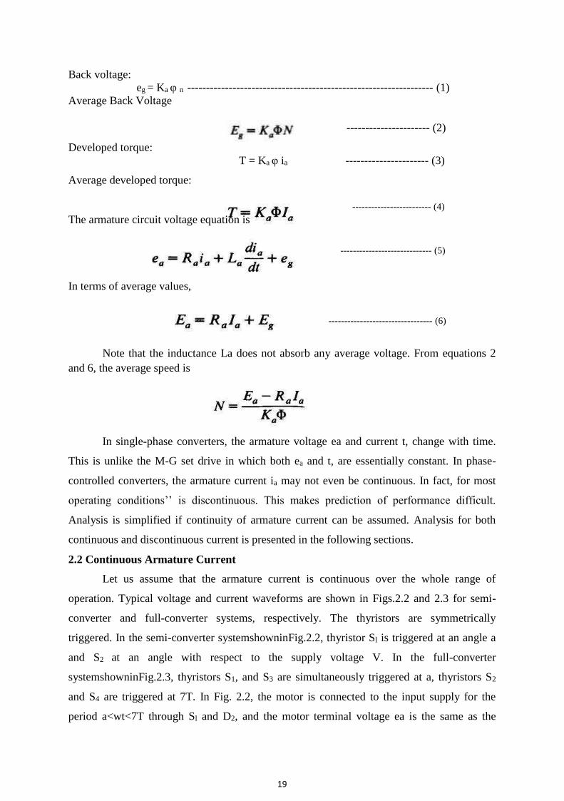
2.2 Continuous Armature Current

Let us assume that the armature current is continuous over the whole range of

operation. Typical voltage and current waveforms are shown in Figs.2.2 and 2.3 for semi-

converter and full-converter systems, respectively. The thyristors are symmetrically

triggered. In the semi-converter systemshowninFig.2.2, thyristor Sl is triggered at an angle a

and S2 at an angle with respect to the supply voltage V. In the full-converter

systemshowninFig.2.3, thyristors S1, and S3 are simultaneously triggered at a, thyristors S2

and S4 are triggered at 7T. In Fig. 2.2, the motor is connected to the input supply for the

period a<wt<7T through Sl and D2, and the motor terminal voltage ea is the same as the

20

supply input voltage V. Beyond 7T, ea tends to reverse as the input voltage changes polarity.

This will forward-bias the free-wheeling diode and DFW will start conducting. The motor

current ia, which was flowing from the supply through Sl' is transferred to DFW (i.e., Sl

commutates). The motor terminals are shorted through the free-wheeling diode during 7T

<wt < (7T +a), making eo zero. Energy from the supply is therefore delivered to the armature

Circuit when the thyristor conducts (a to7T). This energy is partially stored in the

inductance, partially stored in the kinetic energy (K.E.) of the moving system, and partially

used to supply the mechanical load. During the free-wheeling period, 7T to7T +a, energy is

recovered from the inductance and is converted to mechanical form to supplement the K.E.in

supplying the mechanical load. The free-wheeling armature current continues to produce

electromagnetic torque in the motor. No energy is feedback to the supply during this period.

Figs.2.2 and 2.3

21

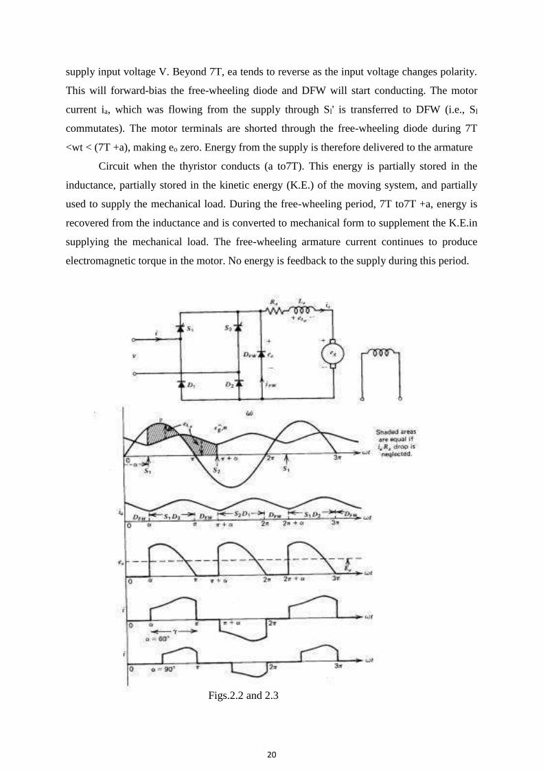
In Fig.2.3, the motor is always connected to the input supply through the thyristors.

Thyristors Sl and S3conduct during the interval a<wt <(7T +a) and connect the motor to the

supply. At 7T +a, thyristors S2 and S4 are triggered. Immediately the supply voltage appears

across the thyristors Sl and S3 as a reverse-bias voltage and turns them off. This is called

natural or line commutation.

The motor current ia, which was flowing from the supply through Sl and S3 'is

transferred to S2and S4. During at 7T, energy flows from the input supply to the motor (both v

and ia repositive, and eo and io are positive, signifying positive power flow). However, during

7T to 7T +a, some of the motor system energy is feedback to the input supply (v and I have

opposite polarities and likewise ea and io' signifying reverse power flow).

In Fig.2.3c voltage and current waveforms are shown for a firing angle greater than

90°.The average motor terminal voltage Eo is negative. If the motor back emf Eg is reversed,

it will behave as a de-generator and will feed power back to the ac supply. This is known as

the inversion operation of the converter, and this mode of operation is used in the

regenerative braking of the motor.

22

2.2.1. Torque Speed Characteristics

For a semi-converter with free-wheeling action the armature circuit equations are: 2.2.2. Single-Phase Separately Excited DC Motor Drives

The armature circuit equation for a full-converter is: 2.3. DISCONTINUOUS ARMATURE CURRENT

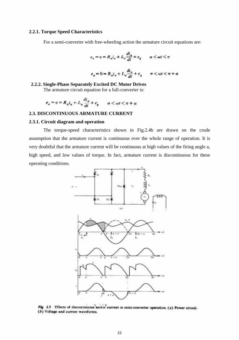
2.3.1. Circuit diagram and operation

The torque-speed characteristics shown in Fig.2.4b are drawn on the crude

assumption that the armature current is continuous over the whole range of operation. It is

very doubtful that the armature current will be continuous at high values of the firing angle a,

high speed, and low values of torque. In fact, armature current is discontinuous for these

operating conditions.

23

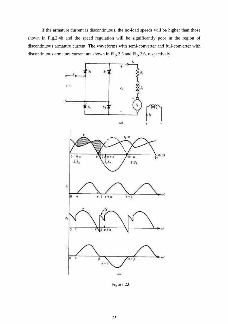
If the armature current is discontinuous, the no-load speeds will be higher than those

shown in Fig.2.4b and the speed regulation will be significantly poor in the region of

discontinuous armature current. The waveforms with semi-converter and full-converter with

discontinuous armature current are shown in Fig.2.5 and Fig.2.6, respectively.

Figure.2.6

24

In Fig. 2.5, the motor is connected to the input supply for the period a<wI <71'

through S, and Dz. Beyond 71', the motor terminal is shorted through the free-wheeling diode

DFW' The armature current decays to zero at before the thyristor S2 is triggered at71' +a,

thereby making the armature current discontinuous. During at 71' (i.e., the conduction period

of the thyristor S,), motor terminal voltage ea is the same as the supply voltage v.

However, during the motor current free-wheels through DFW ea is zero. The motor

coasts and the motor terminal voltage ea is the same as the back voltage InFig.2.6, the motor

is connected to the supply during a<wt<t3 and it Coasts during {3<wI <71' +a. As long as the

motor is connected to the supply, its terminal voltage is the same as the input supply voltage.

If the armature current can be assumed to be continuous, the torque-speed

characteristics can be calculated merely from average values of the motor terminal voltage

and current. In the discontinuous current mode, these calculations are cumbersome. The

difficulty arises in the calculation of the average motor terminal voltage Ea, because (called

the extinction angle, the instant at which the thyristor or motor current becomes zero)

depends on, the average speed N, average armature current la' and the firing angle a. A

general approach, valid for both continuous and discontinuous armature current, is necessary.

2.4. Three Phase Fully Controlled Converter Fed Separately Excited D.C Motor Drive

Three phase controlled rectifiers are used in large power DC motor drives. Three

phase controlled rectifier gives more number of voltages per cycle of supply frequency. This

makes motor current continuous and filter requirement also less.

The number of voltage pulses per cycle depends upon the number of thyristors and

their connections for three phase controlled rectifiers. In three phase drives, the armature

circuit is connected to the output of a three phase controlled rectifier.

Three phase drives are used for high power applications up to megawatts power level.

The ripple frequency of armature voltage is greater than that of the single phase drives and its

requires less inductance in the armature circuit to reduce the armature current ripple

Three phase full converter are used in industrial application up to 1500KW drives. It

is a two quadrant converter.

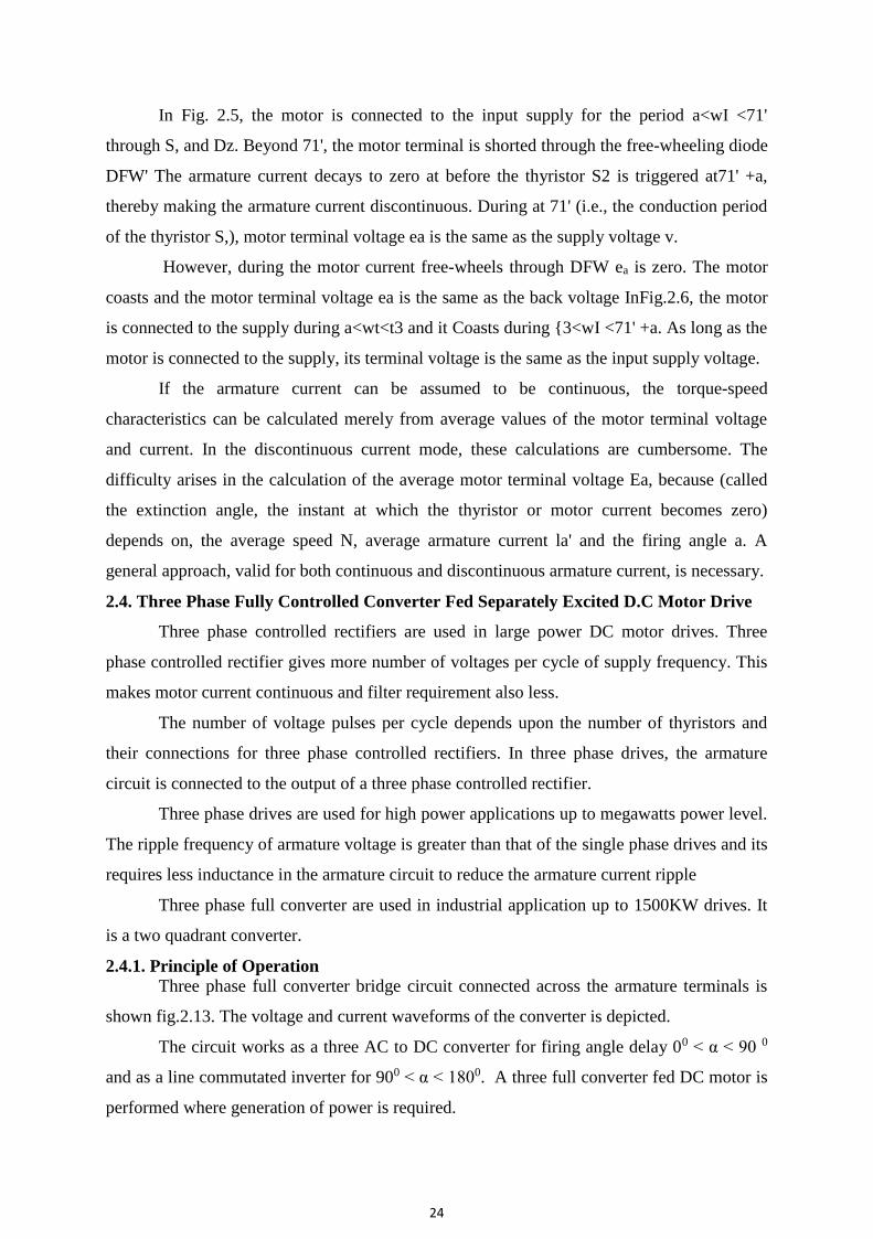
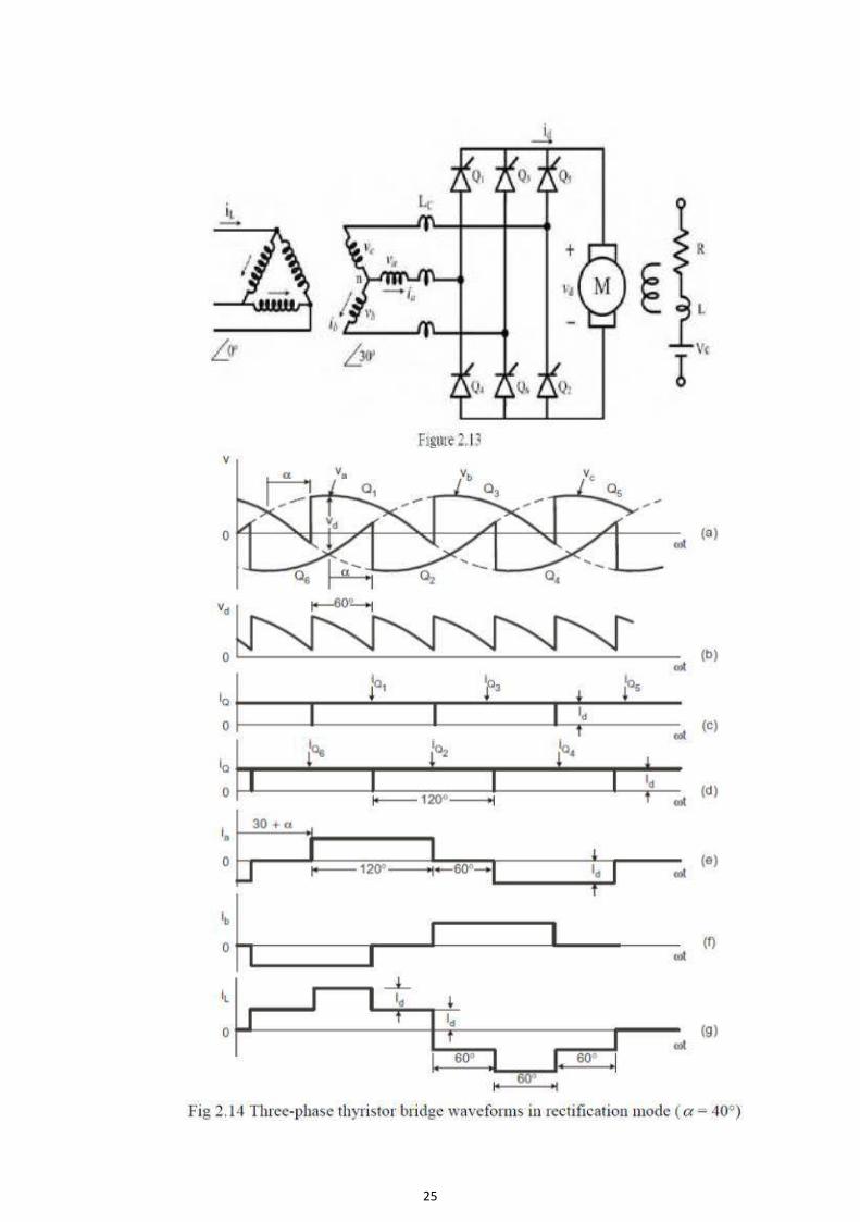
2.4.1. Principle of Operation Three phase full converter bridge circuit connected across the armature terminals is

shown fig.2.13. The voltage and current waveforms of the converter is depicted.

The circuit works as a three AC to DC converter for firing angle delay 00 < α < 90 0

and as a line commutated inverter for 900 < α < 1800. A three full converter fed DC motor is

performed where generation of power is required.

25

26

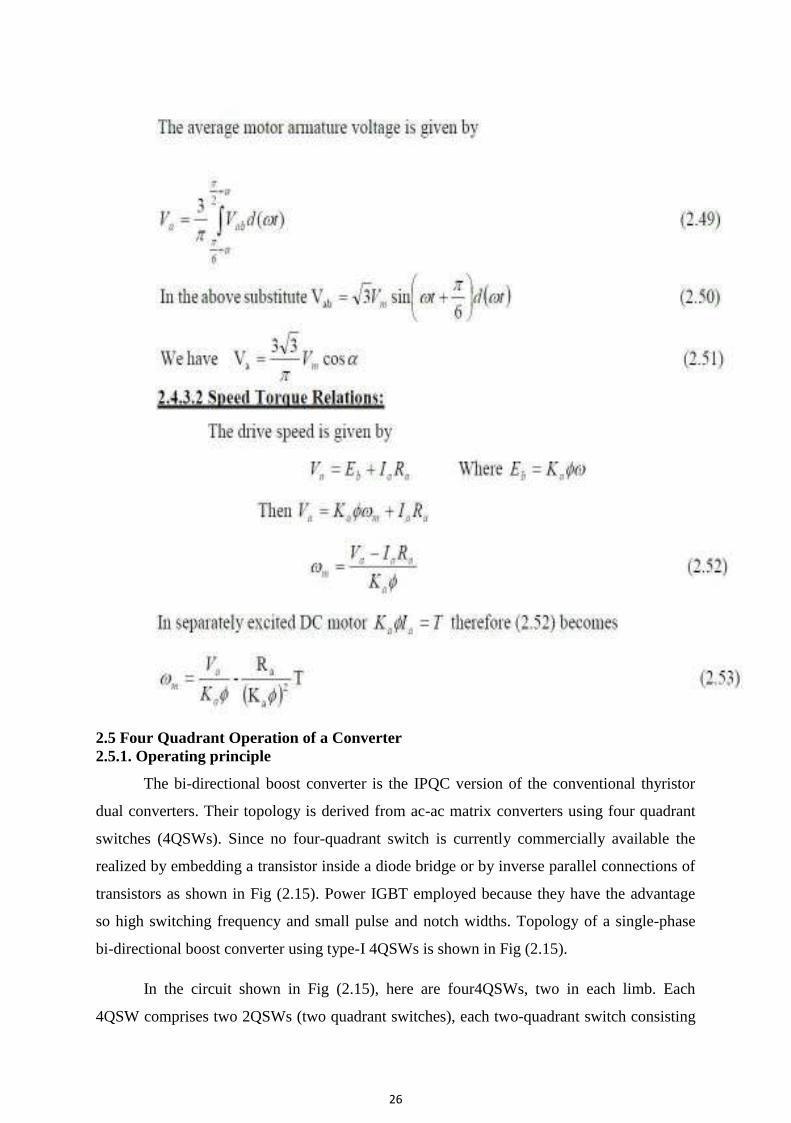
2.5 Four Quadrant Operation of a Converter 2.5.1. Operating principle

The bi-directional boost converter is the IPQC version of the conventional thyristor

dual converters. Their topology is derived from ac-ac matrix converters using four quadrant

switches (4QSWs). Since no four-quadrant switch is currently commercially available the

realized by embedding a transistor inside a diode bridge or by inverse parallel connections of

transistors as shown in Fig (2.15). Power IGBT employed because they have the advantage

so high switching frequency and small pulse and notch widths. Topology of a single-phase

bi-directional boost converter using type-I 4QSWs is shown in Fig (2.15).

In the circuit shown in Fig (2.15), here are four4QSWs, two in each limb. Each

4QSW comprises two 2QSWs (two quadrant switches), each two-quadrant switch consisting

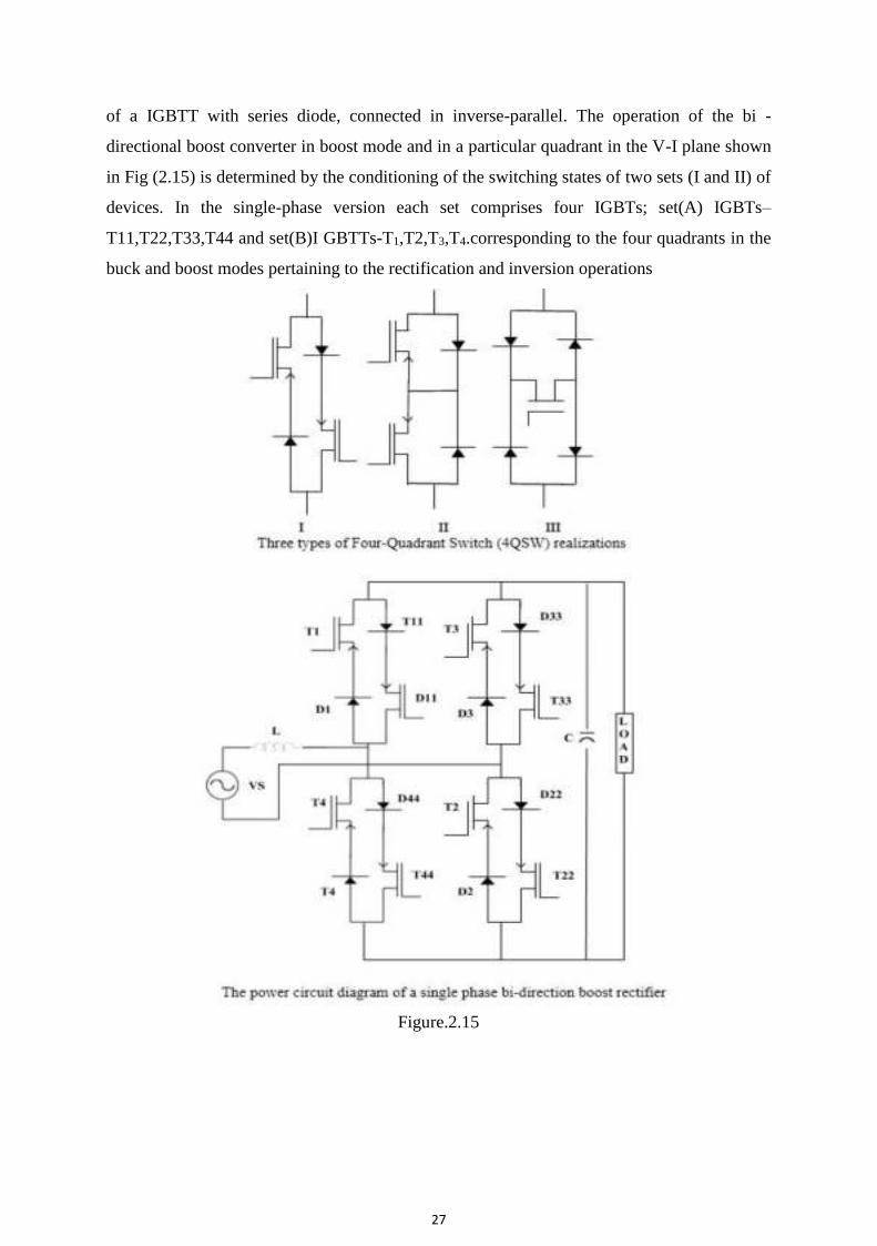
27

of a IGBTT with series diode, connected in inverse-parallel. The operation of the bi -

directional boost converter in boost mode and in a particular quadrant in the V-I plane shown

in Fig (2.15) is determined by the conditioning of the switching states of two sets (I and II) of

devices. In the single-phase version each set comprises four IGBTs; set(A) IGBTs–

T11,T22,T33,T44 and set(B)I GBTTs-T1,T2,T3,T4.corresponding to the four quadrants in the

buck and boost modes pertaining to the rectification and inversion operations

Figure.2.15

28

2.6 Time Ratio Control (TRC)

In this control scheme, time ratio Ton/T (duty ratio) is varied. This is realized by two

different ways called Constant Frequency System and Variable Frequency System as

described below:

2.6.1. Constant Frequency System

In this scheme, on-time is varied but chopping frequency f is kept constant. Variation

of Ton means adjustment of pulse width, as such this scheme is also called pulse-width-

modulation scheme.

2.6.2. Variable Frequency System

In this technique, the chopping frequency f is varied and either

• On-time Ton is kept constant or

• Off-time Toff is kept constant. This method of controlling duty ratio is also called

Frequency-modulation scheme. 2.7 Current- Limit Control

2.7.1. Theory of operation

In this control strategy, the on and off of chopper circuit is decided by the previous set

value of load current. The two set values are maximum load current and minimum load

current.

When the load current reaches the upper limit, chopper is switched off. When the load

current falls below lower limit, the chopper is switched on. Switching frequency of chopper

can be controlled by setting maximum and minimum level of current.

Current limit control involves feedback loop, the trigger circuit for the chopper is

therefore more complex. PWM technique is the commonly chosen control strategy for the

power control in chopper circuit.

29

UNIT III

INDUCTION MOTOR DRIVES

3.1. Stator Voltage Control

3.1.1. Construction and operation

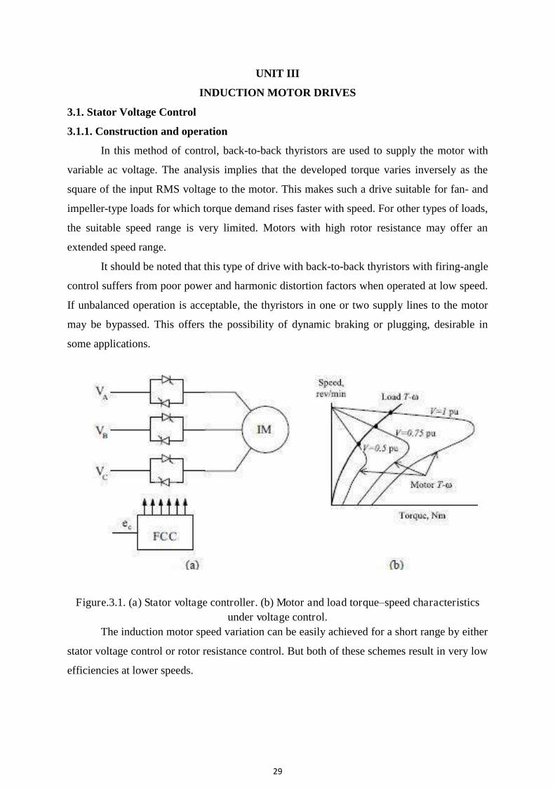
In this method of control, back-to-back thyristors are used to supply the motor with

variable ac voltage. The analysis implies that the developed torque varies inversely as the

square of the input RMS voltage to the motor. This makes such a drive suitable for fan- and

impeller-type loads for which torque demand rises faster with speed. For other types of loads,

the suitable speed range is very limited. Motors with high rotor resistance may offer an

extended speed range.

It should be noted that this type of drive with back-to-back thyristors with firing-angle

control suffers from poor power and harmonic distortion factors when operated at low speed.

If unbalanced operation is acceptable, the thyristors in one or two supply lines to the motor

may be bypassed. This offers the possibility of dynamic braking or plugging, desirable in

some applications.

Figure.3.1. (a) Stator voltage controller. (b) Motor and load torque–speed characteristics under voltage control.

The induction motor speed variation can be easily achieved for a short range by either

stator voltage control or rotor resistance control. But both of these schemes result in very low

efficiencies at lower speeds.

30

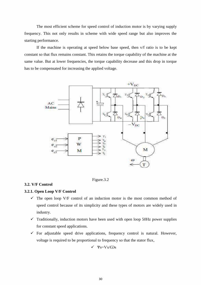
The most efficient scheme for speed control of induction motor is by varying supply

frequency. This not only results in scheme with wide speed range but also improves the

starting performance.

If the machine is operating at speed below base speed, then v/f ratio is to be kept

constant so that flux remains constant. This retains the torque capability of the machine at the

same value. But at lower frequencies, the torque capability decrease and this drop in torque

has to be compensated for increasing the applied voltage.

Figure.3.2 3.2. V/F Control

3.2.1. Open Loop V/F Control

The open loop V/F control of an induction motor is the most common method of

speed control because of its simplicity and these types of motors are widely used in

industry.

Traditionally, induction motors have been used with open loop 50Hz power supplies

for constant speed applications.

For adjustable speed drive applications, frequency control is natural. However,

voltage is required to be proportional to frequency so that the stator flux,

Ѱs=Ѵs/Ѡs

31

Remains constant if the stator resistance is neglected. The power circuit consists of a

diode rectifier with a single or three-phase ac supply, filter and PWM voltage-fed

inverter.

Ideally no feedback signals are required for this control scheme.

The PWM converter is merged with the inverter block. Some problems encountered

in the operation of this open loop drive are the following:

The speed of the motor cannot be controlled precisely, because the rotor speed

will be slightly less than the synchronous speed and that in this scheme the

stator frequency and hence the synchronous speed is the only control variable.

The slip speed, being the difference between the synchronous speed and the

electrical rotor speed, cannot be maintained, as the rotor speed is not measured

in this scheme. This can lead to operation in the unstable region of the torque-

speed characteristics.

The effect of the above can make the stator currents exceed the rated current by a

large amount thus endangering the inverter- converter combination. These problems are to be

suppress by having an outer loop in the induction motor drive, in which the actual rotor speed

is compared with its commanded value, and the error is processed through a controller

usually a PI controller and a limiter is used to obtain the slip-speed command.

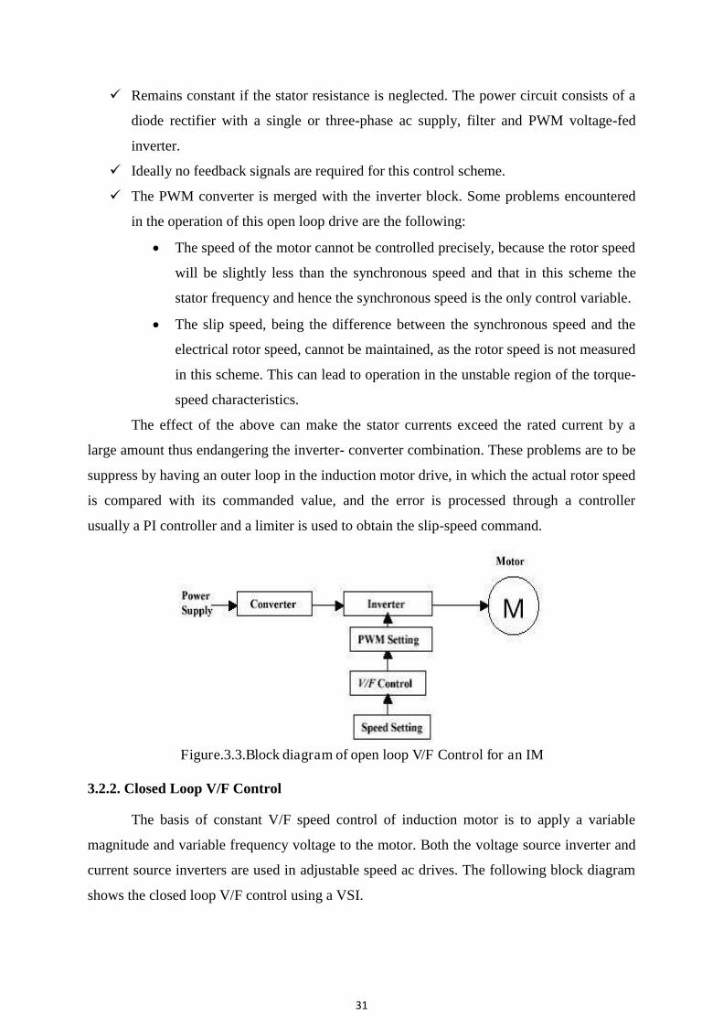
Figure.3.3.Block diagram of open loop V/F Control for an IM

3.2.2. Closed Loop V/F Control

The basis of constant V/F speed control of induction motor is to apply a variable

magnitude and variable frequency voltage to the motor. Both the voltage source inverter and

current source inverters are used in adjustable speed ac drives. The following block diagram

shows the closed loop V/F control using a VSI.

32

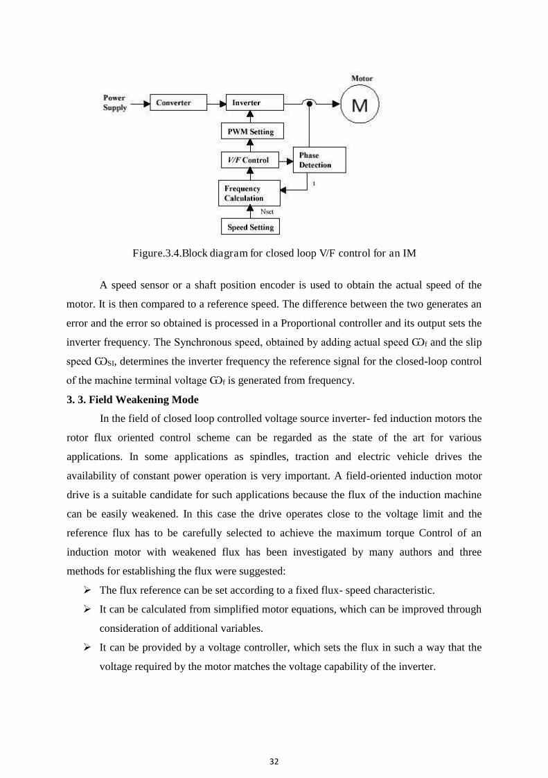
Figure.3.4.Block diagram for closed loop V/F control for an IM

A speed sensor or a shaft position encoder is used to obtain the actual speed of the

motor. It is then compared to a reference speed. The difference between the two generates an

error and the error so obtained is processed in a Proportional controller and its output sets the

inverter frequency. The Synchronous speed, obtained by adding actual speed Ѡf and the slip

speed ѠSI, determines the inverter frequency the reference signal for the closed-loop control

of the machine terminal voltage Ѡf is generated from frequency.

3. 3. Field Weakening Mode

In the field of closed loop controlled voltage source inverter- fed induction motors the

rotor flux oriented control scheme can be regarded as the state of the art for various

applications. In some applications as spindles, traction and electric vehicle drives the

availability of constant power operation is very important. A field-oriented induction motor

drive is a suitable candidate for such applications because the flux of the induction machine

can be easily weakened. In this case the drive operates close to the voltage limit and the

reference flux has to be carefully selected to achieve the maximum torque Control of an

induction motor with weakened flux has been investigated by many authors and three

methods for establishing the flux were suggested:

The flux reference can be set according to a fixed flux- speed characteristic.

It can be calculated from simplified motor equations, which can be improved through

consideration of additional variables.

It can be provided by a voltage controller, which sets the flux in such a way that the

voltage required by the motor matches the voltage capability of the inverter.

33

The third strategy seems to be optimal because it is not sensitive to parameter

variations in a middle speed region. At high speed the current has to be reduced for matching

the maxi - mum torque and for avoiding a pull-out. In this is done with a fixed current-speed

characteristic which is sensitive to parameter and DC link voltage variations. A remedy is

possible if a parameter insensitive feature of the induction machine is used for the current

reduction. Such a criterion is presented and an extension of the voltage control is presented in

this paper which allows an operation with maximum torque in the whole field weakening

region.

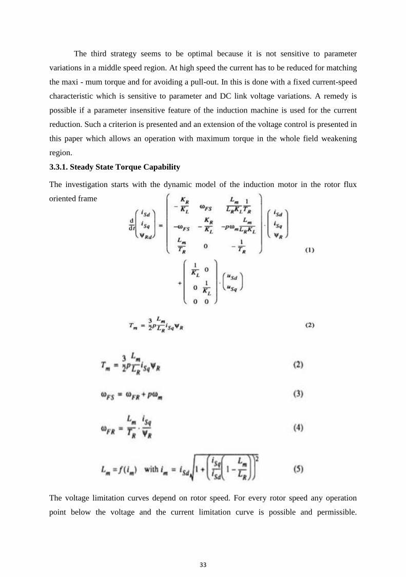
3.3.1. Steady State Torque Capability The investigation starts with the dynamic model of the induction motor in the rotor flux

oriented frame

The voltage limitation curves depend on rotor speed. For every rotor speed any operation

point below the voltage and the current limitation curve is possible and permissible.

34

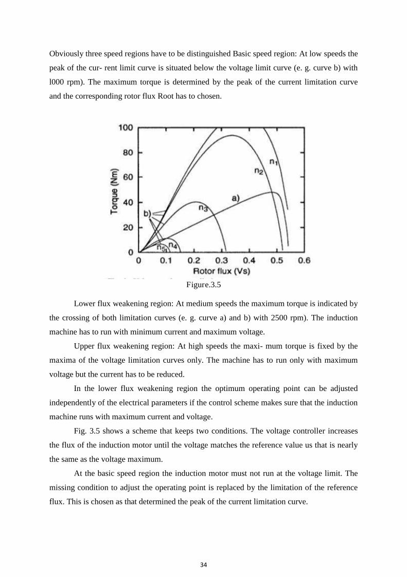
Obviously three speed regions have to be distinguished Basic speed region: At low speeds the

peak of the cur- rent limit curve is situated below the voltage limit curve (e. g. curve b) with

l000 rpm). The maximum torque is determined by the peak of the current limitation curve

and the corresponding rotor flux Root has to chosen.

Figure.3.5

Lower flux weakening region: At medium speeds the maximum torque is indicated by

the crossing of both limitation curves (e. g. curve a) and b) with 2500 rpm). The induction

machine has to run with minimum current and maximum voltage.

Upper flux weakening region: At high speeds the maxi- mum torque is fixed by the

maxima of the voltage limitation curves only. The machine has to run only with maximum

voltage but the current has to be reduced.

In the lower flux weakening region the optimum operating point can be adjusted

independently of the electrical parameters if the control scheme makes sure that the induction

machine runs with maximum current and voltage.

Fig. 3.5 shows a scheme that keeps two conditions. The voltage controller increases

the flux of the induction motor until the voltage matches the reference value us that is nearly

the same as the voltage maximum.

At the basic speed region the induction motor must not run at the voltage limit. The

missing condition to adjust the operating point is replaced by the limitation of the reference

flux. This is chosen as that determined the peak of the current limitation curve.

35

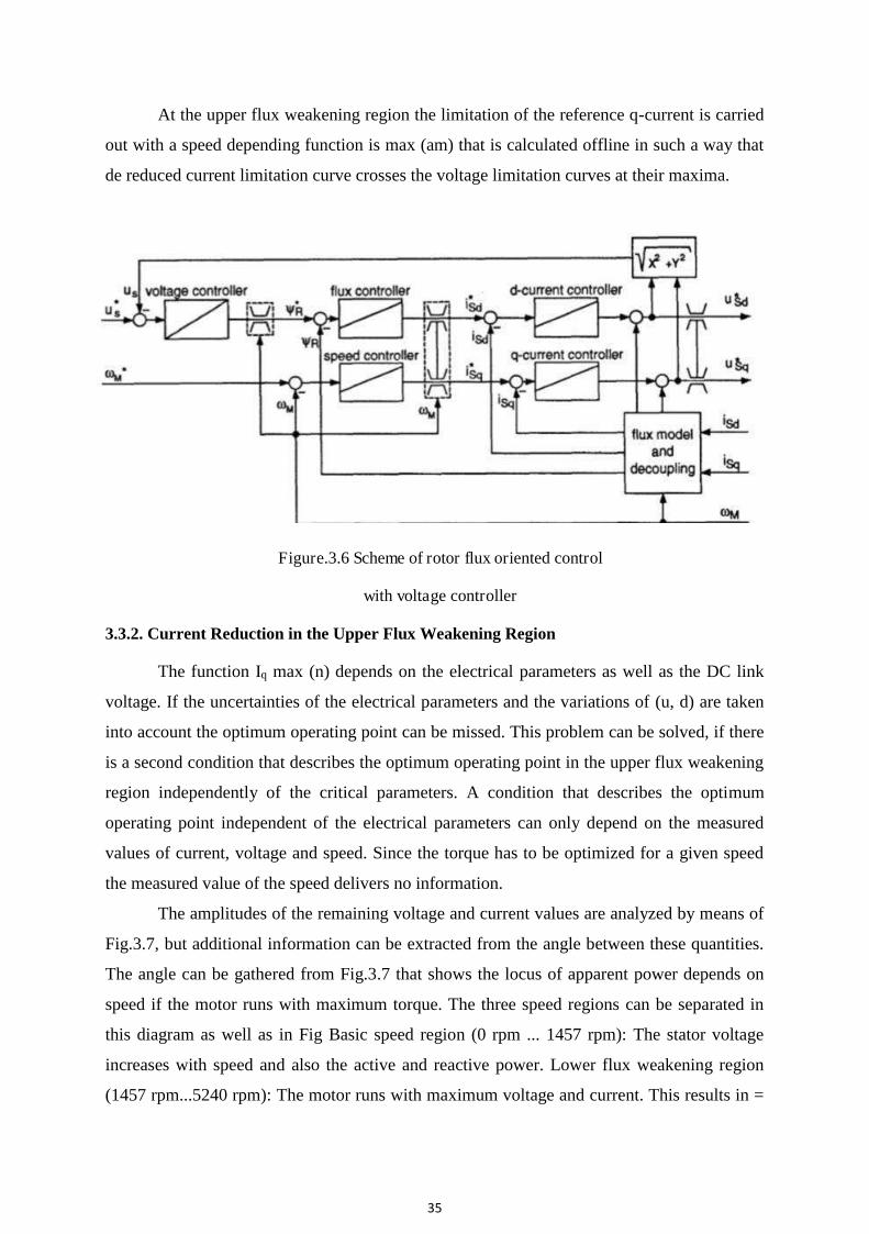
At the upper flux weakening region the limitation of the reference q-current is carried

out with a speed depending function is max (am) that is calculated offline in such a way that

de reduced current limitation curve crosses the voltage limitation curves at their maxima.

Figure.3.6 Scheme of rotor flux oriented control

with voltage controller

3.3.2. Current Reduction in the Upper Flux Weakening Region

The function Iq max (n) depends on the electrical parameters as well as the DC link

voltage. If the uncertainties of the electrical parameters and the variations of (u, d) are taken

into account the optimum operating point can be missed. This problem can be solved, if there

is a second condition that describes the optimum operating point in the upper flux weakening

region independently of the critical parameters. A condition that describes the optimum

operating point independent of the electrical parameters can only depend on the measured

values of current, voltage and speed. Since the torque has to be optimized for a given speed

the measured value of the speed delivers no information.

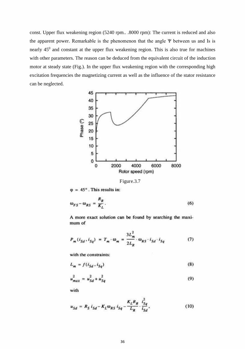
The amplitudes of the remaining voltage and current values are analyzed by means of

Fig.3.7, but additional information can be extracted from the angle between these quantities.

The angle can be gathered from Fig.3.7 that shows the locus of apparent power depends on

speed if the motor runs with maximum torque. The three speed regions can be separated in

this diagram as well as in Fig Basic speed region (0 rpm ... 1457 rpm): The stator voltage

increases with speed and also the active and reactive power. Lower flux weakening region

(1457 rpm...5240 rpm): The motor runs with maximum voltage and current. This results in =

36

const. Upper flux weakening region (5240 rpm.. .8000 rpm): The current is reduced and also

the apparent power. Remarkable is the phenomenon that the angle Ѱ between us and Is is

nearly 450 and constant at the upper flux weakening region. This is also true for machines

with other parameters. The reason can be deduced from the equivalent circuit of the induction

motor at steady state (Fig.). In the upper flux weakening region with the corresponding high

excitation frequencies the magnetizing current as well as the influence of the stator resistance

can be neglected.

Figure.3.7

37

With these equations the torque is maximized for a given rotor speed and not for a

given excitation frequency as with eqn. (6) and in some papers.

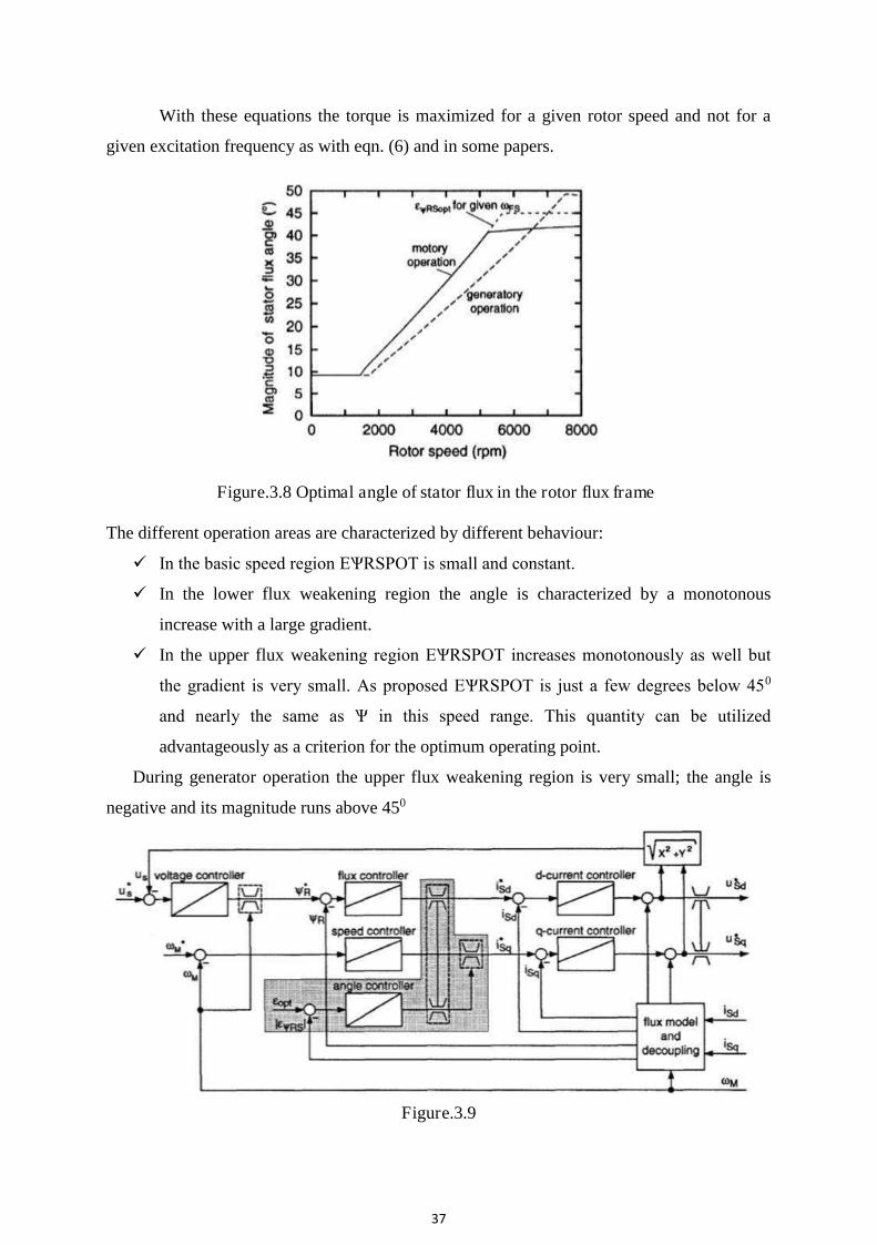
Figure.3.8 Optimal angle of stator flux in the rotor flux frame

The different operation areas are characterized by different behaviour:

In the basic speed region EѰRSPOT is small and constant.

In the lower flux weakening region the angle is characterized by a monotonous

increase with a large gradient.

In the upper flux weakening region EѰRSPOT increases monotonously as well but

the gradient is very small. As proposed EѰRSPOT is just a few degrees below 450

and nearly the same as Ѱ in this speed range. This quantity can be utilized

advantageously as a criterion for the optimum operating point.

During generator operation the upper flux weakening region is very small; the angle is

negative and its magnitude runs above 450

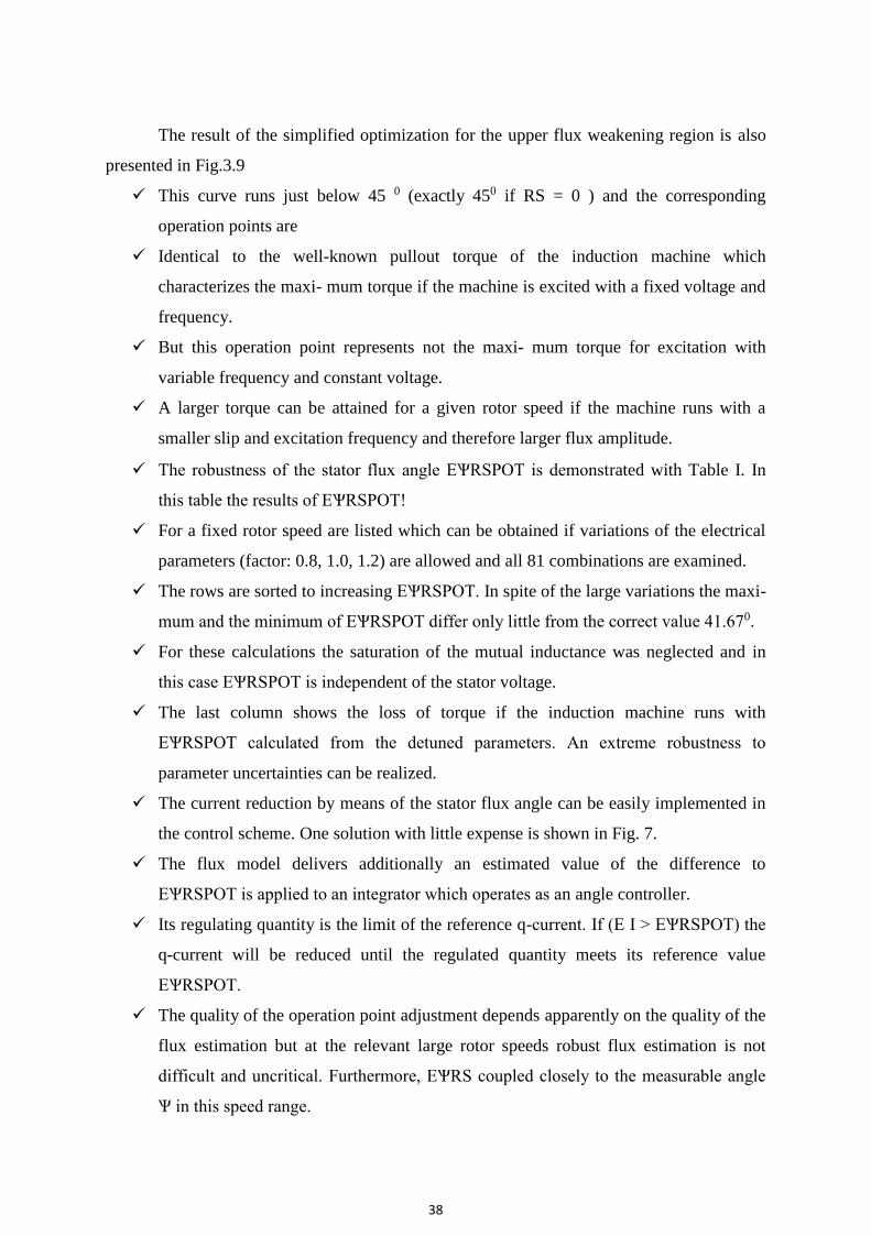
Figure.3.9

38

The result of the simplified optimization for the upper flux weakening region is also

presented in Fig.3.9

This curve runs just below 45 0 (exactly 450 if RS = 0 ) and the corresponding

operation points are

Identical to the well-known pullout torque of the induction machine which

characterizes the maxi- mum torque if the machine is excited with a fixed voltage and

frequency.

But this operation point represents not the maxi- mum torque for excitation with

variable frequency and constant voltage.

A larger torque can be attained for a given rotor speed if the machine runs with a

smaller slip and excitation frequency and therefore larger flux amplitude. The robustness of the stator flux angle EѰRSPOT is demonstrated with Table I. In

this table the results of EѰRSPOT!

For a fixed rotor speed are listed which can be obtained if variations of the electrical

parameters (factor: 0.8, 1.0, 1.2) are allowed and all 81 combinations are examined.

The rows are sorted to increasing EѰRSPOT. In spite of the large variations the maxi-

mum and the minimum of EѰRSPOT differ only little from the correct value 41.670.

For these calculations the saturation of the mutual inductance was neglected and in

this case EѰRSPOT is independent of the stator voltage.

The last column shows the loss of torque if the induction machine runs with

EѰRSPOT calculated from the detuned parameters. An extreme robustness to

parameter uncertainties can be realized.

The current reduction by means of the stator flux angle can be easily implemented in

the control scheme. One solution with little expense is shown in Fig. 7.

The flux model delivers additionally an estimated value of the difference to

EѰRSPOT is applied to an integrator which operates as an angle controller.

Its regulating quantity is the limit of the reference q-current. If (E I > EѰRSPOT) the

q-current will be reduced until the regulated quantity meets its reference value

EѰRSPOT.

The quality of the operation point adjustment depends apparently on the quality of the

flux estimation but at the relevant large rotor speeds robust flux estimation is not

difficult and uncritical. Furthermore, EѰRS coupled closely to the measurable angle

Ѱ in this speed range.

39

3.4. Voltage-source Inverter-driven Induction Motor

A three-phase variable frequency inverter supplying an induction motor is shown in

Figure. The power devices are assumed to be ideal switches.

There are two major types of switching schemes for the inverters, namely, square wave

switching and PWM switching.

3.4.1. Square wave inverters

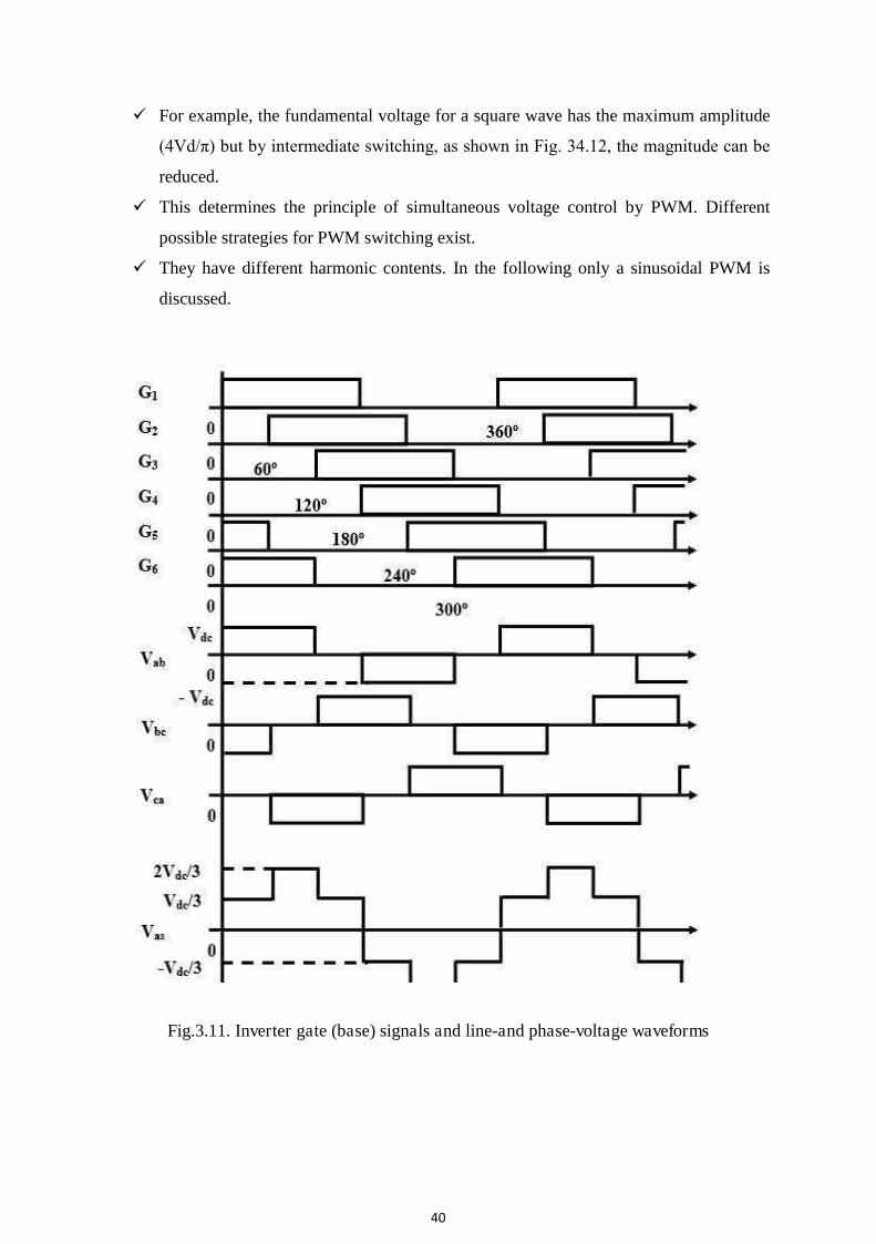
The gating signals and the resulting line voltages for square wave switching are

shown in Figure. The phase voltages are derived from the line voltages assuming a

balanced three-phase system.

Fig.3.10 A schematic of the generic inverter-fed induction motor drive The square wave inverter control is simple and the switching frequency and

consequently, switching losses are low.

However, significant energies of the lower order harmonics and large distortions in

current wave require bulky low-pass filters.

Moreover, this scheme can only achieve frequency control. For voltage control a

controlled rectifier is needed, which offsets some of the cost advantages of the simple

inverter.

3.4.1.1. PWM Principle

It is possible to control the output voltage and frequency of the PWM inverter

simultaneously, as well as optimize the harmonics by performing multiple switching

within the inverter major cycle which determines frequency.

40

For example, the fundamental voltage for a square wave has the maximum amplitude

(4Vd/π) but by intermediate switching, as shown in Fig. 34.12, the magnitude can be

reduced.

This determines the principle of simultaneous voltage control by PWM. Different

possible strategies for PWM switching exist.

They have different harmonic contents. In the following only a sinusoidal PWM is

discussed.

Fig.3.11. Inverter gate (base) signals and line-and phase-voltage waveforms

41

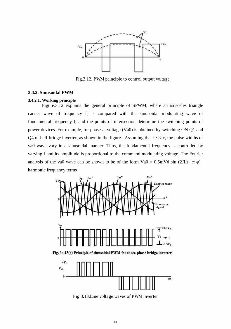
Fig.3.12. PWM principle to control output voltage

3.4.2. Sinusoidal PWM

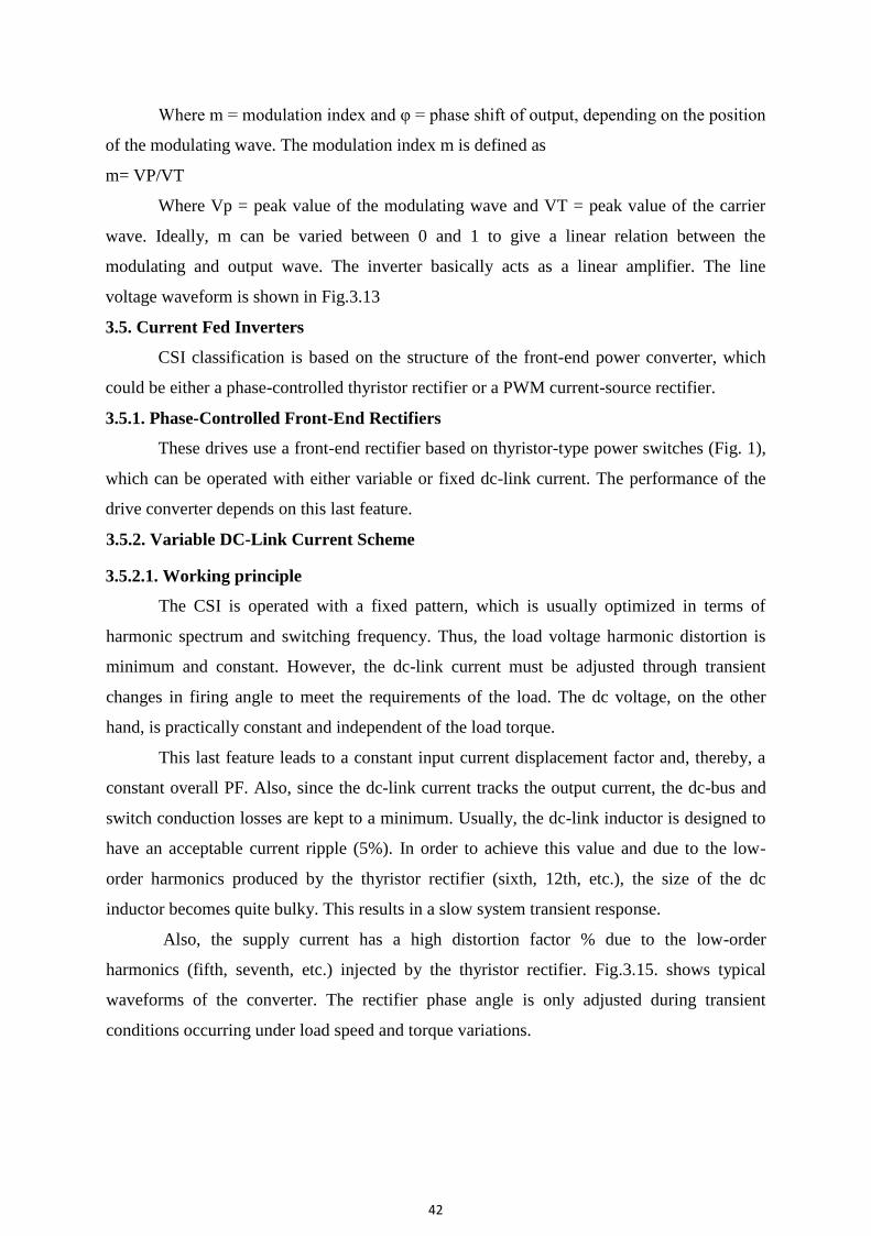
3.4.2.1. Working principle Figure.3.12 explains the general principle of SPWM, where an isosceles triangle

carrier wave of frequency fc is compared with the sinusoidal modulating wave of

fundamental frequency f, and the points of intersection determine the switching points of

power devices. For example, for phase-a, voltage (Va0) is obtained by switching ON Q1 and

Q4 of half-bridge inverter, as shown in the figure . Assuming that f <<fc, the pulse widths of

va0 wave vary in a sinusoidal manner. Thus, the fundamental frequency is controlled by

varying f and its amplitude is proportional to the command modulating voltage. The Fourier

analysis of the va0 wave can be shown to be of the form Va0 = 0.5mVd sin (2Лft +π φ)+

harmonic frequency terms

Fig.3.13.Line voltage waves of PWM inverter

42

Where m = modulation index and φ = phase shift of output, depending on the position

of the modulating wave. The modulation index m is defined as

m= VP/VT

Where Vp = peak value of the modulating wave and VT = peak value of the carrier

wave. Ideally, m can be varied between 0 and 1 to give a linear relation between the

modulating and output wave. The inverter basically acts as a linear amplifier. The line

voltage waveform is shown in Fig.3.13

3.5. Current Fed Inverters

CSI classification is based on the structure of the front-end power converter, which

could be either a phase-controlled thyristor rectifier or a PWM current-source rectifier.

3.5.1. Phase-Controlled Front-End Rectifiers

These drives use a front-end rectifier based on thyristor-type power switches (Fig. 1),

which can be operated with either variable or fixed dc-link current. The performance of the

drive converter depends on this last feature.

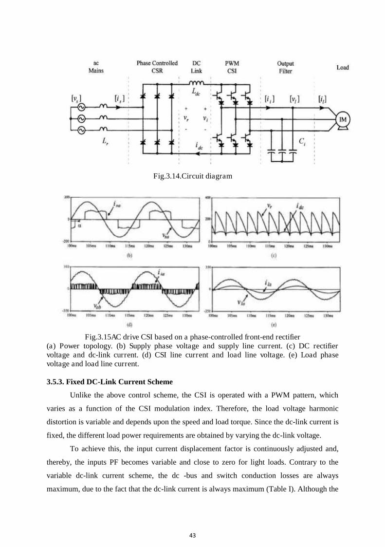
3.5.2. Variable DC-Link Current Scheme 3.5.2.1. Working principle

The CSI is operated with a fixed pattern, which is usually optimized in terms of

harmonic spectrum and switching frequency. Thus, the load voltage harmonic distortion is

minimum and constant. However, the dc-link current must be adjusted through transient

changes in firing angle to meet the requirements of the load. The dc voltage, on the other

hand, is practically constant and independent of the load torque.

This last feature leads to a constant input current displacement factor and, thereby, a

constant overall PF. Also, since the dc-link current tracks the output current, the dc-bus and

switch conduction losses are kept to a minimum. Usually, the dc-link inductor is designed to

have an acceptable current ripple (5%). In order to achieve this value and due to the low-

order harmonics produced by the thyristor rectifier (sixth, 12th, etc.), the size of the dc

inductor becomes quite bulky. This results in a slow system transient response.

Also, the supply current has a high distortion factor % due to the low-order

harmonics (fifth, seventh, etc.) injected by the thyristor rectifier. Fig.3.15. shows typical

waveforms of the converter. The rectifier phase angle is only adjusted during transient

conditions occurring under load speed and torque variations.

43

Fig.3.14.Circuit diagram

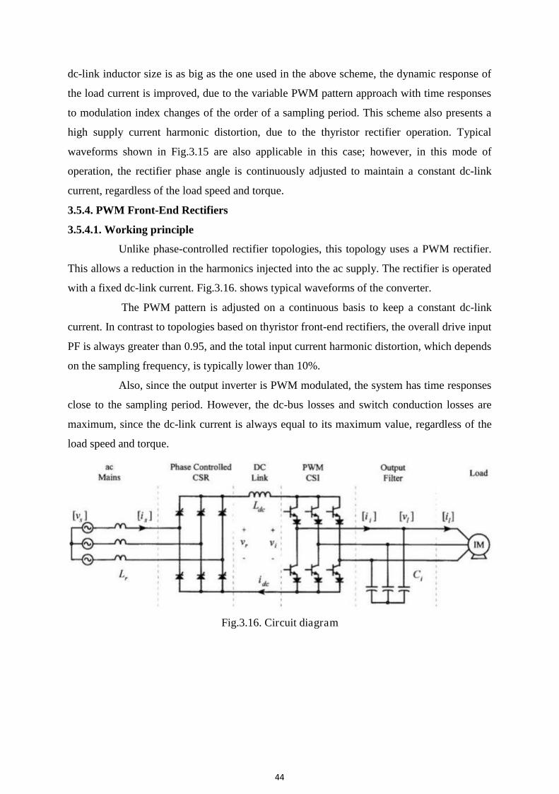
Fig.3.15AC drive CSI based on a phase-controlled front-end rectifier (a) Power topology. (b) Supply phase voltage and supply line current. (c) DC rectifier voltage and dc-link current. (d) CSI line current and load line voltage. (e) Load phase voltage and load line current. 3.5.3. Fixed DC-Link Current Scheme

Unlike the above control scheme, the CSI is operated with a PWM pattern, which

varies as a function of the CSI modulation index. Therefore, the load voltage harmonic

distortion is variable and depends upon the speed and load torque. Since the dc-link current is

fixed, the different load power requirements are obtained by varying the dc-link voltage.

To achieve this, the input current displacement factor is continuously adjusted and,

thereby, the inputs PF becomes variable and close to zero for light loads. Contrary to the

variable dc-link current scheme, the dc -bus and switch conduction losses are always

maximum, due to the fact that the dc-link current is always maximum (Table I). Although the

44

dc-link inductor size is as big as the one used in the above scheme, the dynamic response of

the load current is improved, due to the variable PWM pattern approach with time responses

to modulation index changes of the order of a sampling period. This scheme also presents a

high supply current harmonic distortion, due to the thyristor rectifier operation. Typical

waveforms shown in Fig.3.15 are also applicable in this case; however, in this mode of

operation, the rectifier phase angle is continuously adjusted to maintain a constant dc-link

current, regardless of the load speed and torque.

3.5.4. PWM Front-End Rectifiers

3.5.4.1. Working principle

Unlike phase-controlled rectifier topologies, this topology uses a PWM rectifier.

This allows a reduction in the harmonics injected into the ac supply. The rectifier is operated

with a fixed dc-link current. Fig.3.16. shows typical waveforms of the converter.

The PWM pattern is adjusted on a continuous basis to keep a constant dc-link

current. In contrast to topologies based on thyristor front-end rectifiers, the overall drive input

PF is always greater than 0.95, and the total input current harmonic distortion, which depends

on the sampling frequency, is typically lower than 10%.

Also, since the output inverter is PWM modulated, the system has time responses

close to the sampling period. However, the dc-bus losses and switch conduction losses are

maximum, since the dc-link current is always equal to its maximum value, regardless of the

load speed and torque.

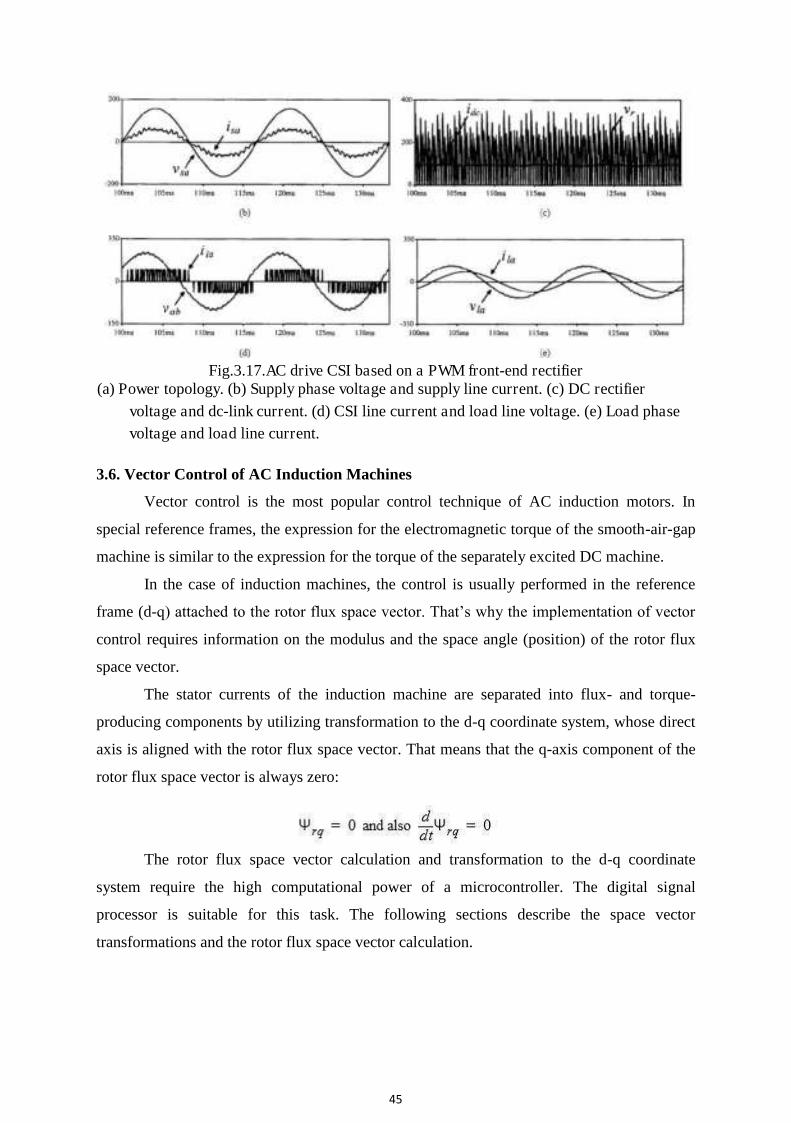
Fig.3.16. Circuit diagram

45

Fig.3.17.AC drive CSI based on a PWM front-end rectifier (a) Power topology. (b) Supply phase voltage and supply line current. (c) DC rectifier

voltage and dc-link current. (d) CSI line current and load line voltage. (e) Load phase voltage and load line current.

3.6. Vector Control of AC Induction Machines

Vector control is the most popular control technique of AC induction motors. In

special reference frames, the expression for the electromagnetic torque of the smooth-air-gap

machine is similar to the expression for the torque of the separately excited DC machine.

In the case of induction machines, the control is usually performed in the reference

frame (d-q) attached to the rotor flux space vector. That’s why the implementation of vector

control requires information on the modulus and the space angle (position) of the rotor flux

space vector.

The stator currents of the induction machine are separated into flux- and torque-

producing components by utilizing transformation to the d-q coordinate system, whose direct

axis is aligned with the rotor flux space vector. That means that the q-axis component of the

rotor flux space vector is always zero:

The rotor flux space vector calculation and transformation to the d-q coordinate

system require the high computational power of a microcontroller. The digital signal

processor is suitable for this task. The following sections describe the space vector

transformations and the rotor flux space vector calculation.

46

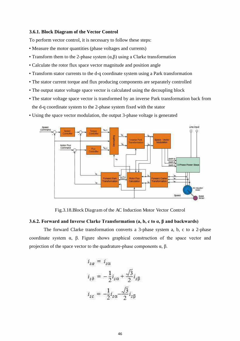
3.6.1. Block Diagram of the Vector Control

To perform vector control, it is necessary to follow these steps:

• Measure the motor quantities (phase voltages and currents)

• Transform them to the 2-phase system (α,β) using a Clarke transformation

• Calculate the rotor flux space vector magnitude and position angle

• Transform stator currents to the d-q coordinate system using a Park transformation

• The stator current torque and flux producing components are separately controlled

• The output stator voltage space vector is calculated using the decoupling block

• The stator voltage space vector is transformed by an inverse Park transformation back from

the d-q coordinate system to the 2-phase system fixed with the stator

• Using the space vector modulation, the output 3-phase voltage is generated

Fig.3.18.Block Diagram of the AC Induction Motor Vector Control 3.6.2. Forward and Inverse Clarke Transformation (a, b, c to α, β and backwards)

The forward Clarke transformation converts a 3-phase system a, b, c to a 2-phase

coordinate system α, β. Figure shows graphical construction of the space vector and

projection of the space vector to the quadrature-phase components α, β.

47

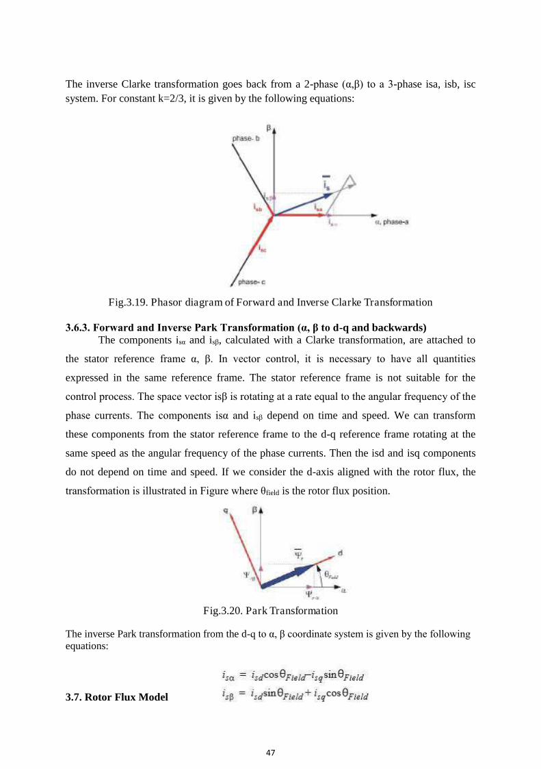
The inverse Clarke transformation goes back from a 2-phase (α,β) to a 3-phase isa, isb, isc system. For constant k=2/3, it is given by the following equations:

Fig.3.19. Phasor diagram of Forward and Inverse Clarke Transformation 3.6.3. Forward and Inverse Park Transformation (α, β to d-q and backwards)

The components isα and isβ, calculated with a Clarke transformation, are attached to

the stator reference frame α, β. In vector control, it is necessary to have all quantities

expressed in the same reference frame. The stator reference frame is not suitable for the

control process. The space vector isβ is rotating at a rate equal to the angular frequency of the

phase currents. The components isα and isβ depend on time and speed. We can transform

these components from the stator reference frame to the d-q reference frame rotating at the

same speed as the angular frequency of the phase currents. Then the isd and isq components

do not depend on time and speed. If we consider the d-axis aligned with the rotor flux, the

transformation is illustrated in Figure where θfield is the rotor flux position.

Fig.3.20. Park Transformation The inverse Park transformation from the d-q to α, β coordinate system is given by the following equations:

3.7. Rotor Flux Model

48

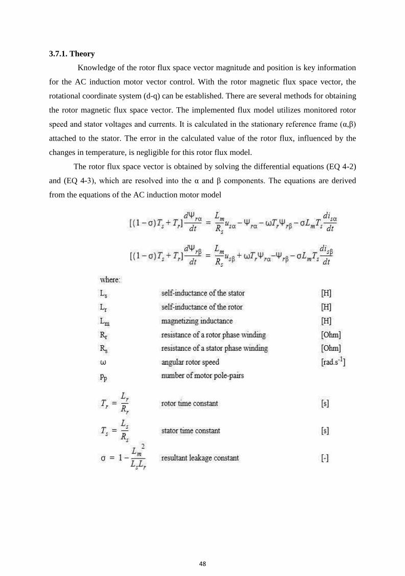
3.7.1. Theory

Knowledge of the rotor flux space vector magnitude and position is key information

for the AC induction motor vector control. With the rotor magnetic flux space vector, the

rotational coordinate system (d-q) can be established. There are several methods for obtaining

the rotor magnetic flux space vector. The implemented flux model utilizes monitored rotor

speed and stator voltages and currents. It is calculated in the stationary reference frame (α,β)

attached to the stator. The error in the calculated value of the rotor flux, influenced by the

changes in temperature, is negligible for this rotor flux model.

The rotor flux space vector is obtained by solving the differential equations (EQ 4-2)

and (EQ 4-3), which are resolved into the α and β components. The equations are derived

from the equations of the AC induction motor model

49

3.8. Closed-loop control of induction motor

3.8.1. Principle of operation

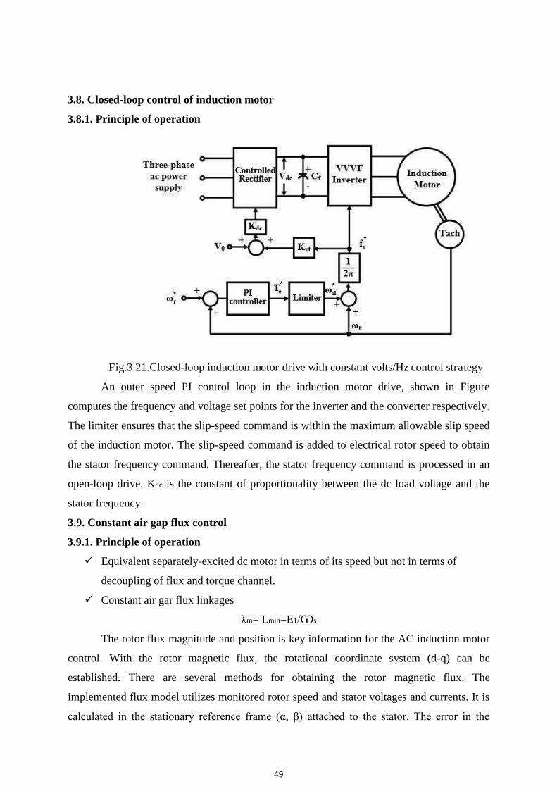
Fig.3.21.Closed-loop induction motor drive with constant volts/Hz control strategy

An outer speed PI control loop in the induction motor drive, shown in Figure

computes the frequency and voltage set points for the inverter and the converter respectively.

The limiter ensures that the slip-speed command is within the maximum allowable slip speed

of the induction motor. The slip-speed command is added to electrical rotor speed to obtain

the stator frequency command. Thereafter, the stator frequency command is processed in an

open-loop drive. Kdc is the constant of proportionality between the dc load voltage and the

stator frequency.

3.9. Constant air gap flux control

3.9.1. Principle of operation

Equivalent separately-excited dc motor in terms of its speed but not in terms of

decoupling of flux and torque channel.

Constant air gar flux linkages

ƛm= Lmin=E1/Ѡs

The rotor flux magnitude and position is key information for the AC induction motor

control. With the rotor magnetic flux, the rotational coordinate system (d-q) can be

established. There are several methods for obtaining the rotor magnetic flux. The

implemented flux model utilizes monitored rotor speed and stator voltages and currents. It is

calculated in the stationary reference frame (α, β) attached to the stator. The error in the

50

calculated value of the rotor flux, influenced by the changes in temperature, is negligible for

this rotor flux model

Fig.3.22Block diagram for constant flux control

51

UNIT IV

SYNCHRONOUS MOTOR DRIVES

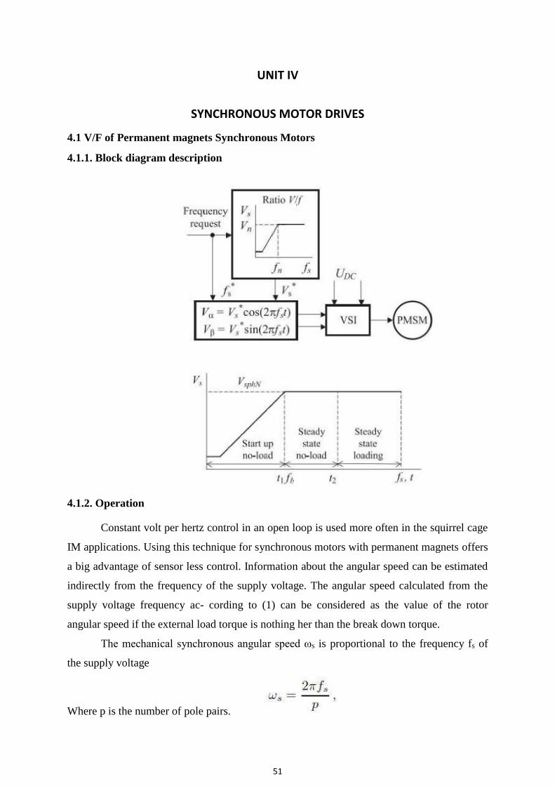
4.1 V/F of Permanent magnets Synchronous Motors 4.1.1. Block diagram description 4.1.2. Operation

Constant volt per hertz control in an open loop is used more often in the squirrel cage

IM applications. Using this technique for synchronous motors with permanent magnets offers

a big advantage of sensor less control. Information about the angular speed can be estimated

indirectly from the frequency of the supply voltage. The angular speed calculated from the

supply voltage frequency ac- cording to (1) can be considered as the value of the rotor

angular speed if the external load torque is nothing her than the break down torque.

The mechanical synchronous angular speed ωs is proportional to the frequency fs of

the supply voltage

Where p is the number of pole pairs.

52

The RMS value of the induced voltage of AC motors is given as

By neglecting the stator resistive voltage drop and as sum- in steady state conditions, the

stator voltage is identical to the induced one and the expression of magnetic flux can be

written as

To maintain the stator flux constant at its nominal value in the base speed range, the

voltage-to-frequency ratio is kept constant, hence the name V/f control. If the ratio is

different from the nominal one, the motor will become overexcited around excited. The first

case happens when the frequency value is lower than the nominal one and the voltage is kept

constant or if the voltage is higher than that of the constant ratio V/f. This condition is called

over excitation, which means that the magnetizing flux is higher than its nominal value.

An increase of the magnetizing flux leads to arise of the magnetizing current. In this

case the hysteresis and eddy current losses are not negligible. The second case represents

under excitation. The motor becomes under excited because the voltage is kept constant and

the value of stator frequency is higher than the nominal one. Scalar control of the

synchronous motor can also be demonstrated via the torque equation of SM, similar to that of

an induction motor. The electromagnetic torque of the synchronous motor, when the stator

resistance Rs is not negligible, is given

The torque will be constant in a wide speed range up to the nominal speed if the ratio

of stator voltage and frequency is kept constant

53

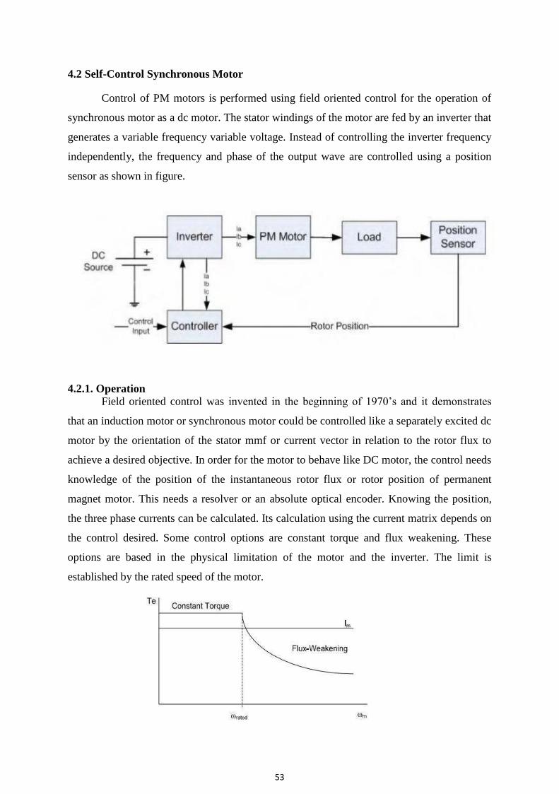
4.2 Self-Control Synchronous Motor

Control of PM motors is performed using field oriented control for the operation of

synchronous motor as a dc motor. The stator windings of the motor are fed by an inverter that

generates a variable frequency variable voltage. Instead of controlling the inverter frequency

independently, the frequency and phase of the output wave are controlled using a position

sensor as shown in figure.

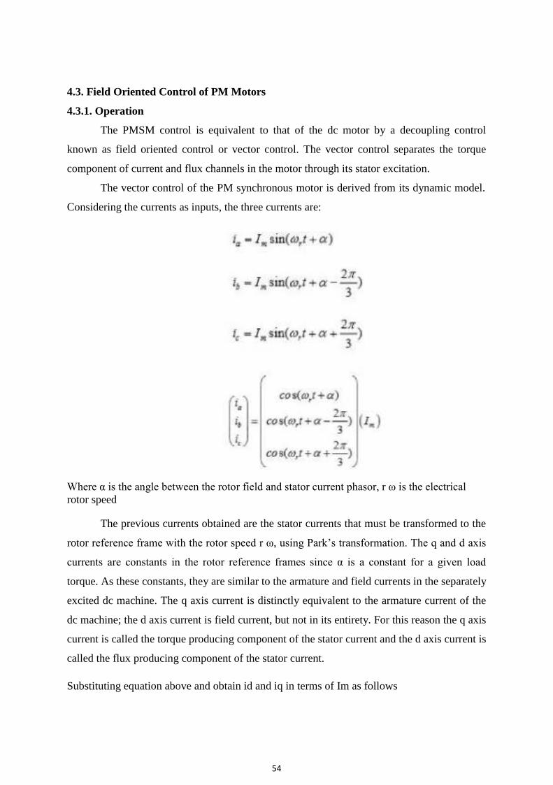
4.2.1. Operation Field oriented control was invented in the beginning of 1970’s and it demonstrates

that an induction motor or synchronous motor could be controlled like a separately excited dc

motor by the orientation of the stator mmf or current vector in relation to the rotor flux to

achieve a desired objective. In order for the motor to behave like DC motor, the control needs

knowledge of the position of the instantaneous rotor flux or rotor position of permanent

magnet motor. This needs a resolver or an absolute optical encoder. Knowing the position,

the three phase currents can be calculated. Its calculation using the current matrix depends on

the control desired. Some control options are constant torque and flux weakening. These

options are based in the physical limitation of the motor and the inverter. The limit is

established by the rated speed of the motor.

54

4.3. Field Oriented Control of PM Motors

4.3.1. Operation

The PMSM control is equivalent to that of the dc motor by a decoupling control

known as field oriented control or vector control. The vector control separates the torque

component of current and flux channels in the motor through its stator excitation.

The vector control of the PM synchronous motor is derived from its dynamic model.

Considering the currents as inputs, the three currents are:

Where α is the angle between the rotor field and stator current phasor, r ω is the electrical rotor speed

The previous currents obtained are the stator currents that must be transformed to the

rotor reference frame with the rotor speed r ω, using Park’s transformation. The q and d axis

currents are constants in the rotor reference frames since α is a constant for a given load

torque. As these constants, they are similar to the armature and field currents in the separately

excited dc machine. The q axis current is distinctly equivalent to the armature current of the

dc machine; the d axis current is field current, but not in its entirety. For this reason the q axis

current is called the torque producing component of the stator current and the d axis current is

called the flux producing component of the stator current.

Substituting equation above and obtain id and iq in terms of Im as follows

55

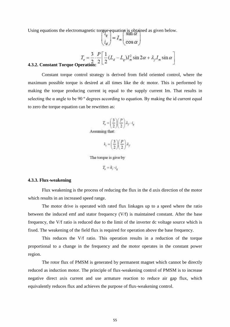
Using equations the electromagnetic torque equation is obtained as given below.

4.3.2. Constant Torque Operation:

Constant torque control strategy is derived from field oriented control, where the

maximum possible torque is desired at all times like the dc motor. This is performed by

making the torque producing current iq equal to the supply current Im. That results in

selecting the α angle to be 90 º degrees according to equation. By making the id current equal

to zero the torque equation can be rewritten as:

4.3.3. Flux-weakening

Flux weakening is the process of reducing the flux in the d axis direction of the motor

which results in an increased speed range.

The motor drive is operated with rated flux linkages up to a speed where the ratio

between the induced emf and stator frequency (V/f) is maintained constant. After the base

frequency, the V/f ratio is reduced due to the limit of the inverter dc voltage source which is

fixed. The weakening of the field flux is required for operation above the base frequency.

This reduces the V/f ratio. This operation results in a reduction of the torque

proportional to a change in the frequency and the motor operates in the constant power

region.

The rotor flux of PMSM is generated by permanent magnet which cannot be directly

reduced as induction motor. The principle of flux-weakening control of PMSM is to increase

negative direct axis current and use armature reaction to reduce air gap flux, which

equivalently reduces flux and achieves the purpose of flux-weakening control.

56

This method changes torque by altering the angle between the stator MMF and the rotor d

axis. In the flux weakening region where ωr>ω rated angle α is controlled by proper control

of id and iq for the same value of stator current. Since iq is reduced the output torque is also

reduced. The angle α can be obtained as:

4.3.3.1. Flux-weakening control realization The realization process of equivalent flux-weakening control is as follows, 1) Measuring rotor position and speed ωr from a sensor which is set in motor rotation axis. 2) The motor at the flux weakening region with a speed loop, Te* is obtained from the PI

controller. 3) Calculate Iq*

4) Calculate Id* using equation: 5) Calculate α using equation 6) Then the current controller makes uses of the reference signals to control the inverter for the desired output currents. 7) The load torque is adjust to the maximum available torque for the reference speed

57

4.4. Power Factor Correction of Permanent Magnet Synchronous Motor Drive With Field Oriented Control Using Space Vector Modulation

Field oriented control demonstrates that, a synchronous motor could be controlled like

a separately excited dc motor by the orientation of the stator mmf or current vector in relation

to the rotor flux to achieve a desired objective.

The aim of the FOC method is to control the magnetic field and torque by controlling

the d and q components of the stator currents or relatively fluxes. With the information of the

stator currents and the rotor angle a FOC technique can control the motor torque and the flux

in a very effective way.

The main advantages of this technique are the fast response and reduced torque ripple.

The implementation of this technique will be carried out using two current regulators, one for

the direct-axis component and another for the quadrature -axis component, and one speed

regulator. There are three PI regulators in the control system. One is for the mechanical

system (speed) and two others for the electrical system (d and q currents).

At first, the reference speed is compared with the measured speed and the error signal

is fed to the speed PI controller.

This regulator compares the actual and reference speed and outputs a torque

command. Once it is obtained, it can be turned into the quadrature-axis current reference, Iqref.

There is a PI controller to regulate the d component of the stator current. The reference value,

Idref, is zero since there is no flux weakening operation. The d component error of the current

is used as an input for the PI regulator.

Moreover, there is another PI controller to regulate the q component of the current.

The reference value is compared with the measured and then fed to the PI regulator.

The performance of the FOC block diagram can be summarized in the following steps:

1. The stator currents are measured as well as the rotor angle.

2. The stator currents are converted into a two-axis reference frame with the Clark

Transformation.

3. The α,β currents are converted into a rotor reference frame using Park Transformation

4. With the speed regulator, a quadrature-axis current reference is obtained. The d-current

controls the air gap flux, the q-current control the torque production.

5. The current error signals are used in controllers to generate reference voltages for the

inverter.

6. The voltage references are turned back into abc domain.

7. With these values are computed the PWM signals required for driving the inverter.

58

4.4.1. SPACE VECTOR MODULATION

The basis of SVPWM is different from that of sine pulse width modulation (SPWM).

SPWM aims to achieve symmetrical 3-phase sine voltage waveforms of adjustable voltage

and frequency, while SVPWM takes the inverter and motor as a whole, using the eight

fundamental voltage vectors to realize variable frequency of voltage and speed adjustment.

SVPWM aims to generate a voltage vector that is close to the reference circle through the

various switching modes of inverter. Fig is the typical diagram of a three-phase voltage

source inverter model.

For the on- off state of the three-phase inverter circuit, every phase can be considered

as a switch S. Here, SA(t), SB(t) and SC(t) are used as the switching functions for the three

phases, respectively.

Diagram of a three phase inverter The space vector of output voltage of inverter can be expressed as,

59

4.5. PMSM Drive with Active Power Factor Correction (Apfc)

4.5.1. PMSM drive with PFC

The above figure shows the block diagram of PMSM drive with Active power Factor

Correction. The APFC consists of an energy stored element, switching device and control

module. It is commonly installed between the power rectifier and the dc link bus. The main

purpose of APFC is to make the input of the power supply look like a pure resistor. In other

words, it is to make the input current waveform in phase with the input voltage waveform so

that there is no phase displacement between them. The operation of APFC is basically based

on a controller that can output the signal to a switching device to control the energy being

stored or released in the reactive elements. In such a way, the input current waveform can be

adjusted. The magnitude and phase of the input current waveforms by proper control can

follow that of the input voltage waveform. Consequently, the power factor improvement can

be achieved and further, the voltage stability can be obtained as well. The dc link voltage for

the inverter is obtained from PFC block. The stator currents and rotor position of PMSM are

given to the FOC, which controls the flux and torque components.

The current error signals are used in controllers to generate reference voltages V α

and Vβ, which are the inputs of SVM. Space Vector modulation gives signals required for

driving the inverter. By using inverter three phase supply is given to the PMSM

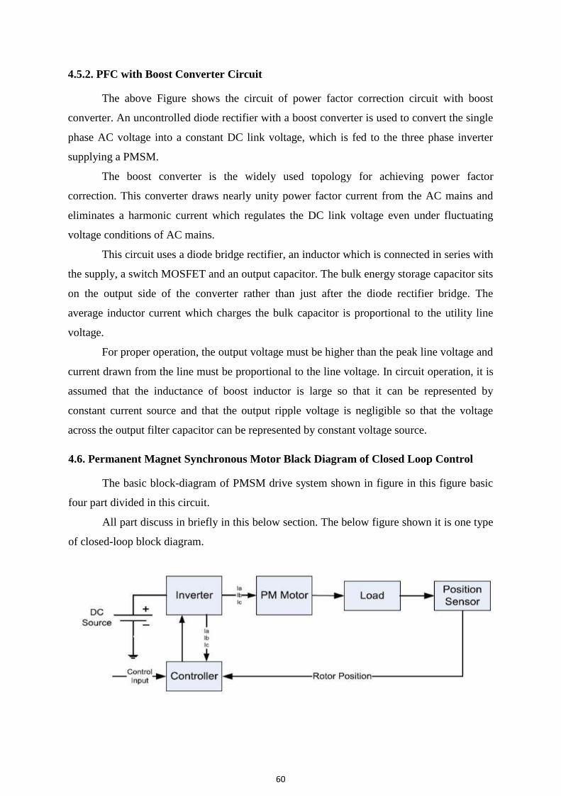
60

4.5.2. PFC with Boost Converter Circuit

The above Figure shows the circuit of power factor correction circuit with boost

converter. An uncontrolled diode rectifier with a boost converter is used to convert the single

phase AC voltage into a constant DC link voltage, which is fed to the three phase inverter

supplying a PMSM.

The boost converter is the widely used topology for achieving power factor

correction. This converter draws nearly unity power factor current from the AC mains and

eliminates a harmonic current which regulates the DC link voltage even under fluctuating

voltage conditions of AC mains.

This circuit uses a diode bridge rectifier, an inductor which is connected in series with

the supply, a switch MOSFET and an output capacitor. The bulk energy storage capacitor sits

on the output side of the converter rather than just after the diode rectifier bridge. The

average inductor current which charges the bulk capacitor is proportional to the utility line

voltage.

For proper operation, the output voltage must be higher than the peak line voltage and

current drawn from the line must be proportional to the line voltage. In circuit operation, it is

assumed that the inductance of boost inductor is large so that it can be represented by

constant current source and that the output ripple voltage is negligible so that the voltage

across the output filter capacitor can be represented by constant voltage source.

4.6. Permanent Magnet Synchronous Motor Black Diagram of Closed Loop Control

The basic block-diagram of PMSM drive system shown in figure in this figure basic

four part divided in this circuit.

All part discuss in briefly in this below section. The below figure shown it is one type

of closed-loop block diagram.

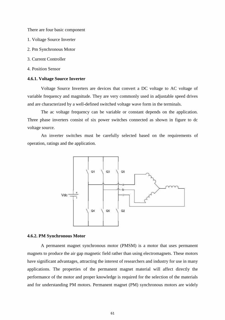
61

There are four basic component 1. Voltage Source Inverter 2. Pm Synchronous Motor 3. Current Controller 4. Position Sensor 4.6.1. Voltage Source Inverter

Voltage Source Inverters are devices that convert a DC voltage to AC voltage of

variable frequency and magnitude. They are very commonly used in adjustable speed drives

and are characterized by a well-defined switched voltage wave form in the terminals.

The ac voltage frequency can be variable or constant depends on the application.

Three phase inverters consist of six power switches connected as shown in figure to dc

voltage source.

An inverter switches must be carefully selected based on the requirements of

operation, ratings and the application.

4.6.2. PM Synchronous Motor

A permanent magnet synchronous motor (PMSM) is a motor that uses permanent

magnets to produce the air gap magnetic field rather than using electromagnets. These motors

have significant advantages, attracting the interest of researchers and industry for use in many

applications. The properties of the permanent magnet material will affect directly the

performance of the motor and proper knowledge is required for the selection of the materials

and for understanding PM motors. Permanent magnet (PM) synchronous motors are widely

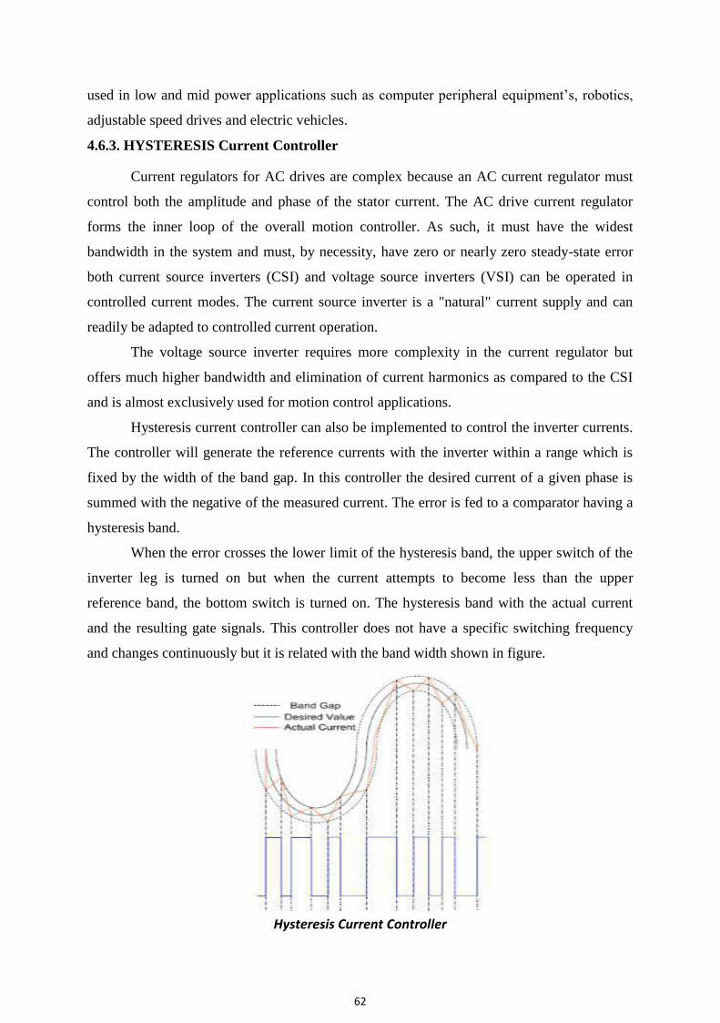
62

used in low and mid power applications such as computer peripheral equipment’s, robotics,

adjustable speed drives and electric vehicles.

4.6.3. HYSTERESIS Current Controller

Current regulators for AC drives are complex because an AC current regulator must

control both the amplitude and phase of the stator current. The AC drive current regulator

forms the inner loop of the overall motion controller. As such, it must have the widest

bandwidth in the system and must, by necessity, have zero or nearly zero steady-state error

both current source inverters (CSI) and voltage source inverters (VSI) can be operated in

controlled current modes. The current source inverter is a "natural" current supply and can

readily be adapted to controlled current operation.

The voltage source inverter requires more complexity in the current regulator but

offers much higher bandwidth and elimination of current harmonics as compared to the CSI

and is almost exclusively used for motion control applications.

Hysteresis current controller can also be implemented to control the inverter currents.

The controller will generate the reference currents with the inverter within a range which is

fixed by the width of the band gap. In this controller the desired current of a given phase is

summed with the negative of the measured current. The error is fed to a comparator having a

hysteresis band.

When the error crosses the lower limit of the hysteresis band, the upper switch of the

inverter leg is turned on but when the current attempts to become less than the upper

reference band, the bottom switch is turned on. The hysteresis band with the actual current

and the resulting gate signals. This controller does not have a specific switching frequency

and changes continuously but it is related with the band width shown in figure.

Hysteresis Current Controller

63

4.6.4. Position Sensor

Operation of permanent magnet synchronous motors requires position sensors in the

rotor shaft when operated without damper winding. The need of knowing the rotor position

requires the development of devices for position measurement. There are four main devices

for the measurement of position, the potentiometer, linear variable differential transformer,

optical encoder and resolvers. The ones most commonly used for motors are encoders and

revolvers. Depending on the application and performance desired by the motor a position

sensor with the required accuracy can be selected.

4.7. VECTOR CONTROL TECHNIQUE

The PMSM control is equivalent to that of the dc motor by a decoupling control

known as field oriented control or vector control. The vector control separates the torque

component of current and flux channels in the motor through its stator excitation. The vector

control strategy is somewhat similar to that of the induction motor vector control, except for

the following:

1. The slip frequency is zero because the machine always runs at synchronous speed.

2. The magnetizing current Ids =0 because the rotor flux is supplied by the PM.

The unit vector generated from an absolute position sensor because, the unlike slipping poles of an induction motor, the poles are fixed on the rotor.

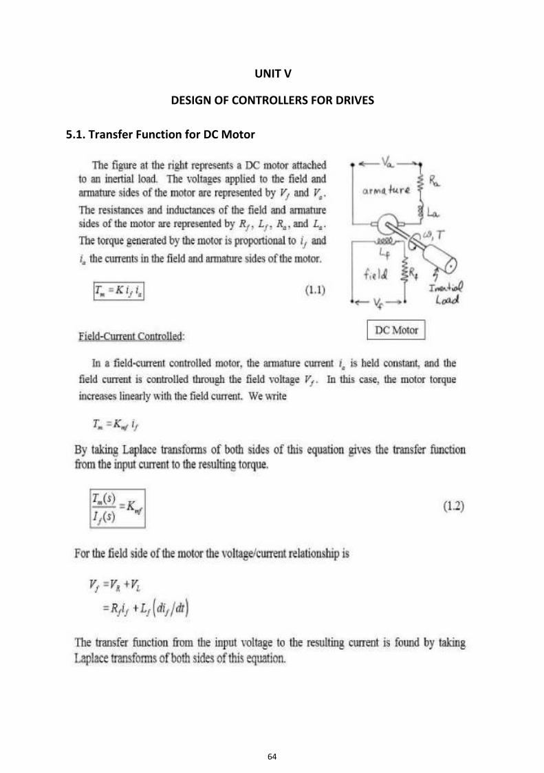
64

UNIT V

DESIGN OF CONTROLLERS FOR DRIVES

5.1. Transfer Function for DC Motor

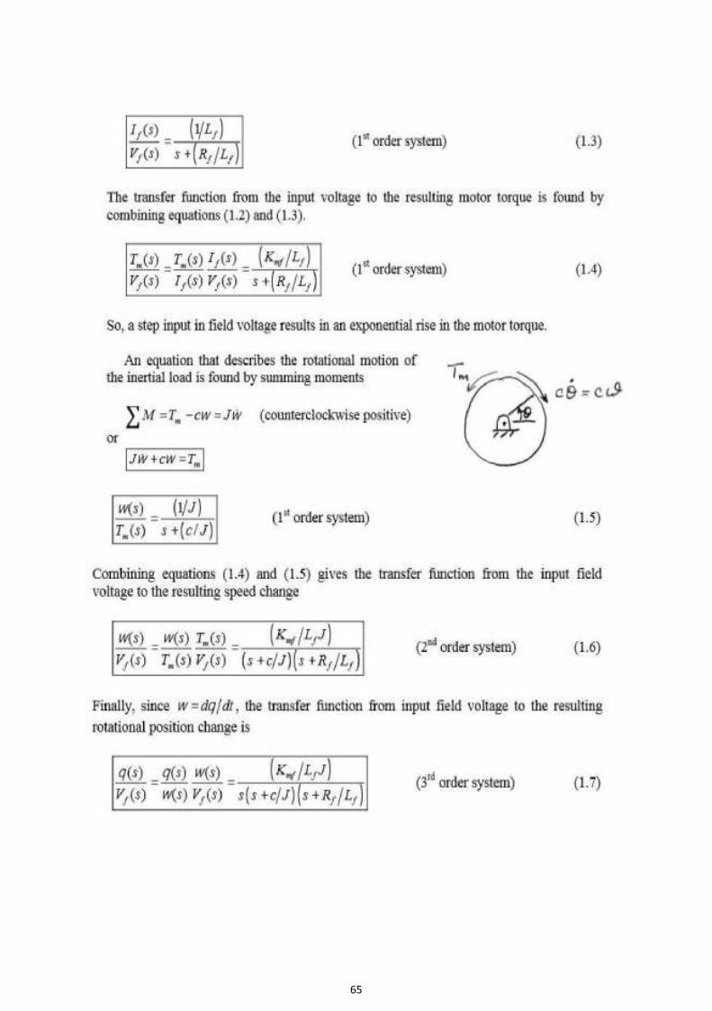
65

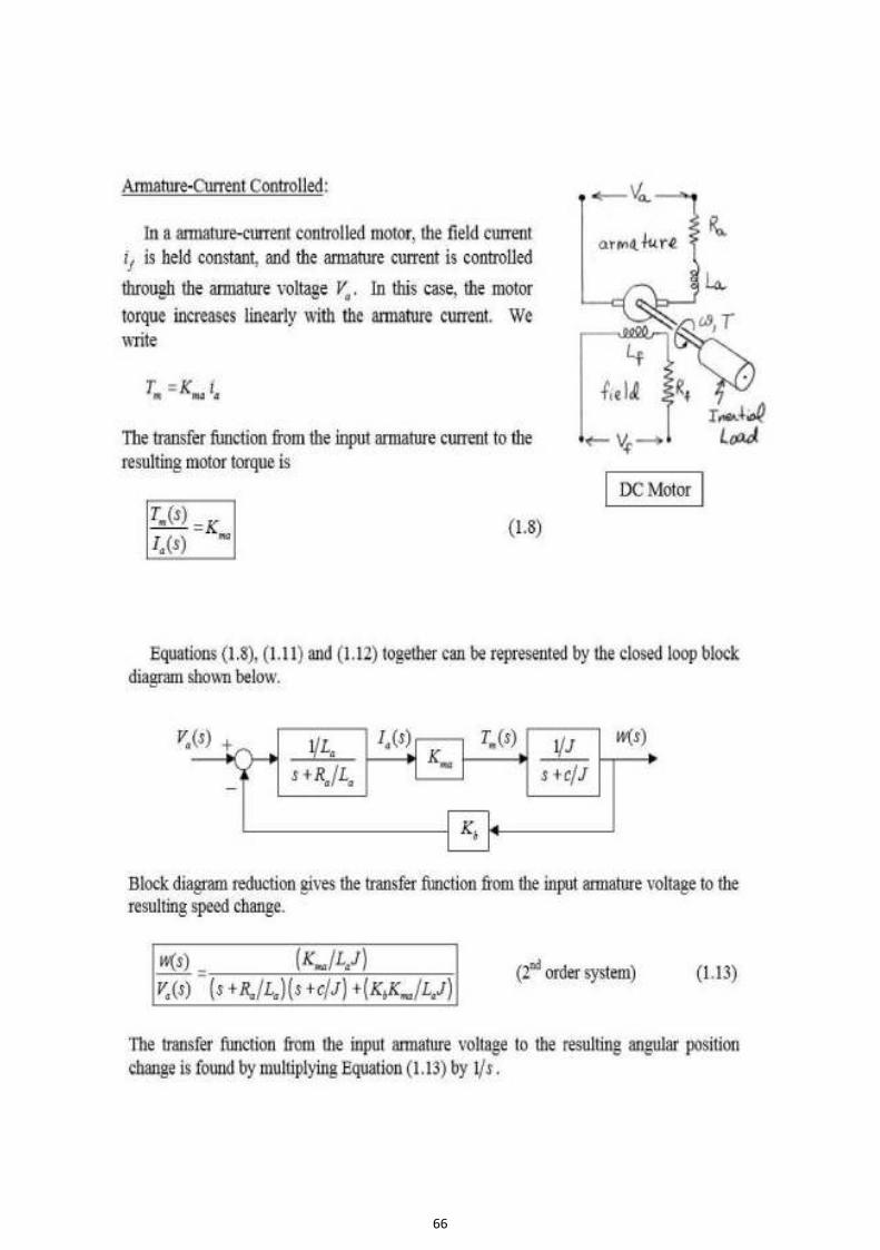
66

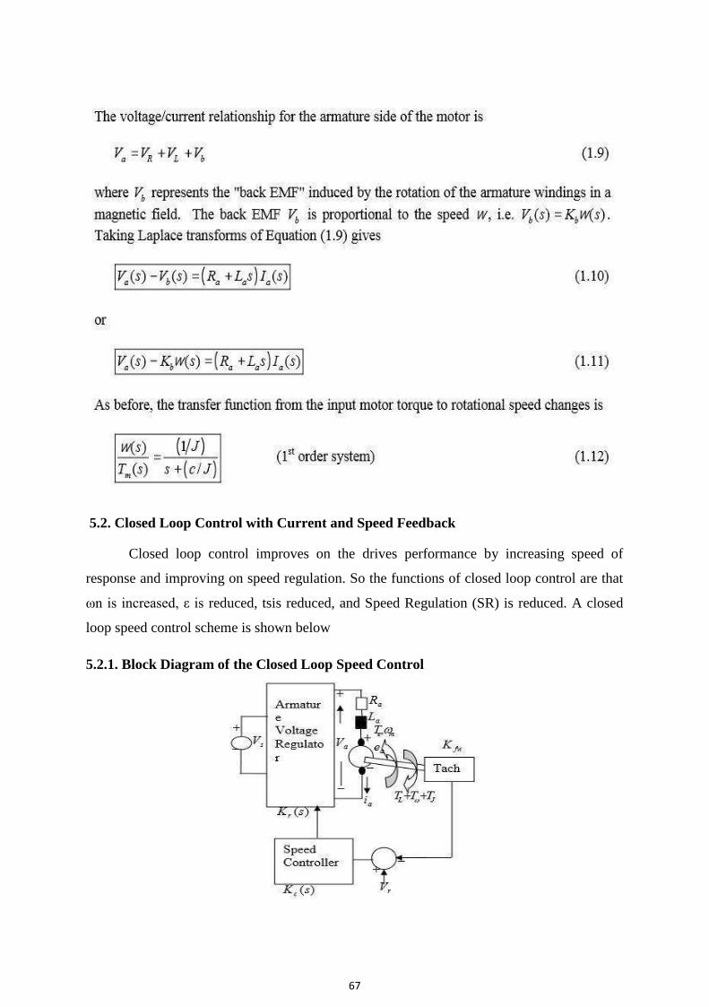
67

5.2. Closed Loop Control with Current and Speed Feedback

Closed loop control improves on the drives performance by increasing speed of

response and improving on speed regulation. So the functions of closed loop control are that

ωn is increased, ε is reduced, tsis reduced, and Speed Regulation (SR) is reduced. A closed

loop speed control scheme is shown below 5.2.1. Block Diagram of the Closed Loop Speed Control

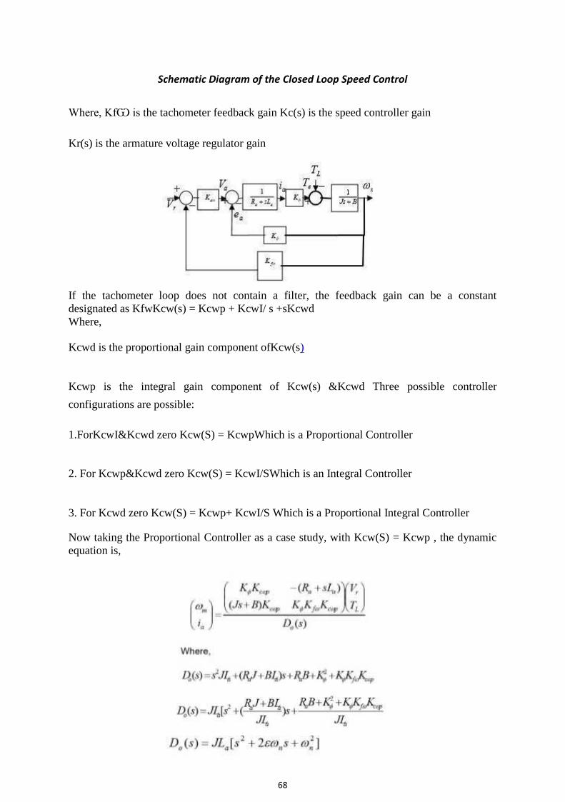
68

Schematic Diagram of the Closed Loop Speed Control

Where, KfѠ is the tachometer feedback gain Kc(s) is the speed controller gain

Kr(s) is the armature voltage regulator gain

If the tachometer loop does not contain a filter, the feedback gain can be a constant designated as KfwKcw(s) = Kcwp + KcwI/ s +sKcwd Where, Kcwd is the proportional gain component ofKcw(s) Kcwp is the integral gain component of Kcw(s) &Kcwd Three possible controller

configurations are possible:

1.ForKcwI&Kcwd zero Kcw(S) = KcwpWhich is a Proportional Controller 2. For Kcwp&Kcwd zero Kcw(S) = KcwI/SWhich is an Integral Controller 3. For Kcwd zero Kcw(S) = Kcwp+ KcwI/S Which is a Proportional Integral Controller Now taking the Proportional Controller as a case study, with Kcw(S) = Kcwp , the dynamic equation is,

69

Last Equation is a second order system The Natural Frequency of Oscillation, ωn is

This is always higher than the open loop case due to the factor

Kф ,KfѠ,KcѠp The Damping Ratio ε , is

This is lower than in the open loop case due to the increase in ωn Speed Regulation (SR) is also derived as

SR is also lower than in the open loop case due to the factor Kф , KfѠ, KcѠp . This is an indication of a better drive performance. 5.2.2.1. Inner Current Loop Control

Improvement in speed control can be obtained with Inner Current Loop Control

method, whereby armature current is fed back to the input.

A closed loop speed control scheme with inner current control is shown in Figure.

Designating K1ci+Kr=Kci

The block diagram representation of the control configuration is shown in Figure.

The dynamic equation is,

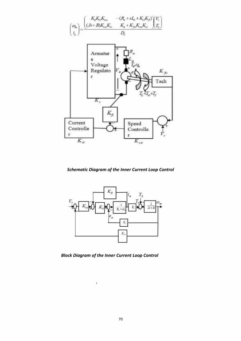
70

Schematic Diagram of the Inner Current Loop Control

Block Diagram of the Inner Current Loop Control

,

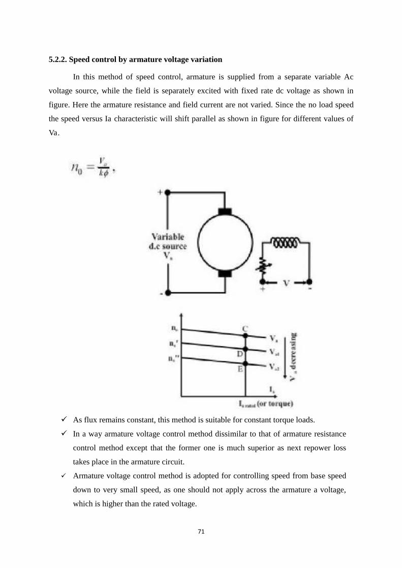
71

5.2.2. Speed control by armature voltage variation

In this method of speed control, armature is supplied from a separate variable Ac

voltage source, while the field is separately excited with fixed rate dc voltage as shown in

figure. Here the armature resistance and field current are not varied. Since the no load speed

the speed versus Ia characteristic will shift parallel as shown in figure for different values of

Va.

As flux remains constant, this method is suitable for constant torque loads.

In a way armature voltage control method dissimilar to that of armature resistance

control method except that the former one is much superior as next repower loss

takes place in the armature circuit.

Armature voltage control method is adopted for controlling speed from base speed

down to very small speed, as one should not apply across the armature a voltage,

which is higher than the rated voltage.

72

5.3. Flux-Weakening Control Design and Analysis

5.3.1. Theory

In order to produce the maximum torque, which main component is proportional to q-

axis component of the armature current, it is convenient to control the inverter-fed PMSM by

keeping the direct, d-axis, current component to be id as long as the inverter output voltage

doesn’t reach its limit.

At that point, the motor reaches its maximum speed, so-called rated speed (called al

so base speed when talking about flux-weakening). Beyond that limit, the motor torque

decreases rapidly toward its minimum value, which depends on a load torque profile. To

expand the speed above the rated value, the motor torque is necessary to be reduced. A

common method in the control of synchronous motors is to reduce the magnetizing current,

which produces the magnetizing flux. This method is known as field-weakening. With PM

synchronous motors it is not possible, but, instead, the air gap flux is weakened by producing

anegative d-axis current component, id.

Because nothing has happened to the excitation magnetic field and the air gap flux is

still reduced, so is the motor torque, this control method is called flux-weakening. As a basis

for this analysis, the PMSM current and voltage d-q vector diagrams from the previous

section Fig are used. During flux-weakening, because the demagnetizing (negative) id current

increases, a phase current vector is rotates toward the negative d-semi-axis.

The rotation of the phase voltage vector is determined by a chosen flux weakening

strategy, but at the end of flux-weakening it always rotates toward the positive q- semi axis

because of iq current, i.e.,vd voltage magnitudedecrease.

Hence, the voltage-to-current phase shift decreases to zero and increases in negative

direction either tothe inverter phase shift limit (usually 300), or a load torque dictated steady-

state (zero acceleration), or to the zero motor torque condition (no load or generative load). A

big concern of flux-weakening control is a danger of permanent demagnetization of magnets.

However, large materials such as Samarium-Cobalt, allows significant id current which can

extend the motor rated speed up to two times. Three commonly used flux-weakening control

strategies are:

1) constant-voltage-constant-power(CVCP)control;

2) constant-current-constant-power(CCCP)control;and

3) Optimum-current-vector(OCVorCCCV-constant-current-constant-voltage)control.

5.4. Design of controller

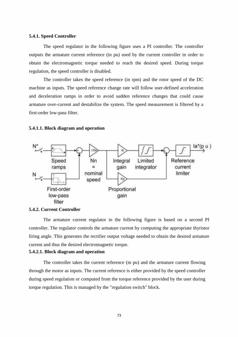
73

5.4.1. Speed Controller

The speed regulator in the following figure uses a PI controller. The controller

outputs the armature current reference (in pu) used by the current controller in order to

obtain the electromagnetic torque needed to reach the desired speed. During torque

regulation, the speed controller is disabled.

The controller takes the speed reference (in rpm) and the rotor speed of the DC

machine as inputs. The speed reference change rate will follow user-defined acceleration

and deceleration ramps in order to avoid sudden reference changes that could cause

armature over-current and destabilize the system. The speed measurement is filtered by a

first-order low-pass filter.

5.4.1.1. Block diagram and operation

5.4.2. Current Controller

The armature current regulator in the following figure is based on a second PI

controller. The regulator controls the armature current by computing the appropriate thyristor

firing angle. This generates the rectifier output voltage needed to obtain the desired armature

current and thus the desired electromagnetic torque.

5.4.2.1. Block diagram and operation

The controller takes the current reference (in pu) and the armature current flowing

through the motor as inputs. The current reference is either provided by the speed controller

during speed regulation or computed from the torque reference provided by the user during

torque regulation. This is managed by the "regulation switch" block.

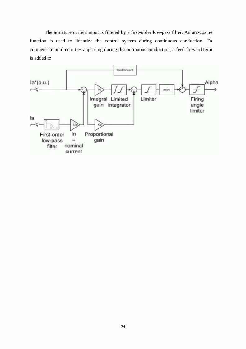
74

The armature current input is filtered by a first-order low-pass filter. An arc-cosine

function is used to linearize the control system during continuous conduction. To

compensate nonlinearities appearing during discontinuous conduction, a feed forward term

is added to