Embed Size (px)
Citation preview

Department of Electrical Power Engineering and
Mechatronics
ULTRA LOW POWER SENSOR FOR MONITORING STRUCTURES VIBRATION
ÜLIMADALA VOOLUTARBEGA VIBRATSIOONISENSOR EHITISTE
MONITOORIMISEKS
MASTER THESIS
Student: RAMY EZZAT
Student code MAHM 165575
Supervisor: MART TAMRE PROFESSOR
Tallinn, 2019

2
(On the reverse side of title page)
AUTHOR’S DECLARATION
Hereby I declare, that I have written this thesis independently.
No academic degree has been applied for based on this material. All works, major viewpoints and
data of the other authors used in this thesis have been referenced.
20TH MAY 2019
Author: RAMY EZZAT
/signature /
Thesis is in accordance with terms and requirements
20TH MAY 2019
Supervisor: MART TAMRE
/signature/
Accepted for defence
20TH MAY 2019.
Chairman of theses defence commission: .............................................................................
/name and signature/
DEPARTMENT OF ELECTRICAL POWER ENGINEERING AND MECHATRONICS

3
THESIS TASK Student: RAMY EZZAT; MAHM 165575
Study programme: MAHM; MECHATRONICS MSc
main speciality: ……………………………………
Supervisor(s): Professor MART TAMRE, Head of Mechatronics TTÜ
Consultants: LEEVI PÕLDARU, Product Developer
Company: NORDIC AUTOMATION SYSTEMS, +372 504 2568, [email protected]
Thesis topic:
(in English) Ultra-low power sensor for monitoring structures vibration
(in Estonian) Ülimadala voolutarbega vibratsioonisensor ehitiste monitoorimiseks
Thesis main objectives:
1. Simple study of structures behaviour upon vibrations
2. Configuring a sensor to monitor structures vibration fits to LoRaWAN technology
3. Analyse real samples (4. Build a rigid library in C/C++)
Thesis tasks and time schedule:
No Task description Deadline
1. Vibration sensing research 1st March
2. Sensor design/configuration 1st April
3. Sensor adjustment 1st April
5. Documentation and presentation 10th May
Language: English Deadline for submission of thesis: “.......” .................... 201…. a
Student: RAMY EZZAT .....................…….............. “.......” .................... 201…. a
/signature/
Supervisor: MART TAMRE ………….............................. “.......” ...................... 201 …. a
/signature/
Consultant: LEEVI PÕLDARU …………........................... “.......” ...................... 201 …. a
/signature/
Terms of thesis closed defence and/or restricted access conditions to be formulated on the reverse
side

4
CONTENTS PREFACE .............................................................................................................................. 7
List of abbreviations and symbols ......................................................................................... 8
INTRODUCTION ................................................................................................................. 9
1 REVIEW ........................................................................................................................... 12
1.1 Vibration nature ......................................................................................................... 12
1.2 Current available solution .......................................................................................... 13
1.3 Current solution discussion advantages and disadvantages ...................................... 14
1.4 Technologies used ..................................................................................................... 14
1.4.1 Vibration sensing technology ..................................................................................... 15
1.4.2 LoRa technology ........................................................................................................ 16
2 METHODOLOGY ........................................................................................................... 17
2.1 Approach justification ............................................................................................... 18
2.1.1 Limitations to structures ............................................................................................. 19
2.1.2 Sensor selection .......................................................................................................... 22
2.1.3 Sensors comparison .................................................................................................... 27
2.1.4 Sensor’s uncertainty ................................................................................................... 32
2.1.5 Communications ......................................................................................................... 34
2.2 Implementation .......................................................................................................... 35
2.2.1 Data acquisition .......................................................................................................... 36
2.2.2 Data logging ............................................................................................................... 39
2.2.3 Data analysis and manipulation .................................................................................. 41
2.2.4 Acquired data referencing .......................................................................................... 49
2.2.5 Power consumption management ............................................................................... 52
2.3 Success measurement ................................................................................................ 55
2.4 Data acquisition, code and sensor library manipulation ............................................ 55
3 RESULTS ......................................................................................................................... 56
4 DISCUSSION ................................................................................................................... 59
5 CONCLUSION ................................................................................................................ 60
SUMMARY ........................................................................................................................ 61
LIST OF REFERENCES .................................................................................................... 63
APPENDICES ..................................................................................................................... 64

5
Table of figures Figure 1. Transient vibration guide values for cosmetic damage, source: BS 7385-2 ........ 20
Figure 2. simplified top view of the Analog Devices ADXL50 MEMS sensor a passive, linear
accelerometer, source: [8] chapter 7- 7.3.1.14 micromachined IC accelerometer ............ 23
Figure 3. piezoelectric accelerometer, source: [9] ............................................................. 24
Figure 4. piezo resistive accelerometer, source: [9] ........................................................... 25
Figure 5. variable inductance accelerometer, source: [9] .................................................. 25
Figure 6. hall effect accelerometer, source: [9] .................................................................. 26
Figure 7. distance, velocity, and acceleration of simple harmonic oscillation, source [1] . 27
Figure 8. sensor’s SPI MOSI signal, source: oscilloscope output ........................................ 37
Figure 9. sensor’s serial clock signal, source: oscilloscope output ..................................... 38
Figure 10. jumper wire connection error, source: google images ...................................... 38
Figure 11. sensor container schematic, source: created via draw.io ................................. 39
Figure 12. acquisition program flow chart, source: created via draw.io ............................ 40
Figure 13. sensor ODR of 105 Hz (1), source: DMM output ............................................... 42
Figure 14. sensor ODR at 105 Hz (2), source: DMM output ............................................... 42
Figure 15. three axes 32,74 k sensor samples, source: python analysis script .................. 43
Figure 16. 300 samples extracted out, source: python analysis script ............................... 44
Figure 17. 14 k sensor samples, source: python analysis script ......................................... 45
Figure 18. samples of 100 first, source: python analysis script .......................................... 46
Figure 19. samples of 100 second, source: python analysis script ..................................... 47
Figure 20. vibrational events of the 14 k samples, source: python analysis script ............ 48
Figure 21. VibSensor referenced acquired data, source: VibSensor mobile app ............... 49
Figure 22. VibSensor referenced acquired data analysed using python script, source:
python analysis script .......................................................................................................... 50
Figure 23. sensor’s data acquired to be referenced, source: python analysis script ......... 51
Figure 24. LoRaWAN power consumption estimation, source: calculated ........................ 53

6
Table of tables Table 1. Transient vibration guide values for cosmetic damage, source: BS 7385-2 ......... 19
Table 2. Damage Classification, source: BS 7385-1:1990 ................................................... 20
Table 3. vibrations effects on structures, source: [6] Part 3 ............................................... 22
Table 4. sensitivity with respect to full range ..................................................................... 30
Table 5. range and minimum sensitivity ............................................................................. 31
Table 6. Uncertainty calculations from referenced readings at [2.2.4] ............................... 32
Table 7. sensor output line example ................................................................................... 41
Table 8. approximation of current consumption ................................................................ 53
Table of equations Equation 1. ........................................................................................................................... 27
Equation 2. ........................................................................................................................... 27
Equation 3. ........................................................................................................................... 27
Equation 4. ........................................................................................................................... 28
Equation 5. ........................................................................................................................... 28
Equation 6. ........................................................................................................................... 28
Equation 7. ........................................................................................................................... 29
Equation 8. ........................................................................................................................... 31
Equation 9. ........................................................................................................................... 32
Equation 10. ......................................................................................................................... 32
Equation 11. ......................................................................................................................... 33
Equation 12. ......................................................................................................................... 33
Equation 13. ......................................................................................................................... 33
Equation 14. ......................................................................................................................... 33
Equation 15. ......................................................................................................................... 33

7
PREFACE Between the following pages there is a research of achieving an ultra-low power sensor that can
monitor structures vibrations, a sensor that can estimate if vibrations happened or about to happen
are within the standard range limit of structures safety standards.
A research of solutions available in the market and their advantages and disadvantages and know-
how of building this device that can monitor structures vibrations, what are the limits of those
vibrations, how strong or fast they can get so that structure can withstand, what are the available
sensors in the market that can measure and assess those vibrations with the best accuracy possible
and least cost and power consumption, and how to manipulate that sensor to achieve the best
results out of it.
The work of this research has been done at Nordic automation systems, where, I work as a
mechatronics engineer and which has adopted the idea as it’s in the scope of our development to
produce ultra-low power IoT devices that can communicate over a very secured, long range, and
low power RF communication protocol LoRaWAN that works as end-to-end.
For that I would like to thank NAS for giving me the opportunity to develop that product as it has
expanded my experience which has made me recall most of my studies and taught me new
technologies and information, and thanks for everyone that has shared a recommendation of to
do or don’t in development, for that I would like to thank my development team in the NAS, and
moreover I would like to thank whoever supported me to go further in this research and motivated
me to accomplish it as it is, for all of you I appreciate it and express my sincere gratitude.

8
List of abbreviations and symbols
LoRaWAN long range wide area network
LPWA low power wide are wireless
PPV peak particle velocity
PPA peak particle acceleration
MEMS micro-electro-mechanical systems
LSB least significant bit
SPI serial peripheral interface
I2C inter-integrated circuit - I square C
bps byte per second
MOSI master output slave input
MISO master input slave output
SCLK serial clock
SS slave select
USB universal serial bus
CSV comma separated values
MCU microcontroller unit
IoT internet of things
FFT fast Fourier transform
DAQ data acquisition
DK development kit
SDK software development kit
ODR output data rate
DMM digital multi-meter
IDE integrated development environment
NAS Nordic automation systems
LP low power
ULP ultra-low power
SHM simple harmonic motion
RF radio frequency

9
INTRODUCTION
Buildings have existed since human first steps on earth, human build structures to stay safe, well
sheltered from whatever danger nature might bring, wild animals, bad weather etc.
And consequently, it’s needed to keep these buildings safe specially if they are hospitals or if
they’re ancient and historic structures, or if their construction process was resources-expensive,
or hard to maintain.
The second most destructive uncontrollable phenomenon that can ever be a threat for structures
is vibrations; besides that, the first uncontrollable thing threating structures is natural disasters,
which can be harsh sometime and lead to structures destruction.
Therefore, there is a need for a solution to monitor structures from vibrations happening or about
to happen, a vibration detection device can be used for such need, it shall be used by structures
owners to monitor vibrations happening to their buildings, or for construction sites producing
high vibration and needs to monitor their produced vibration.
So, the main problem being addressed here, is monitoring structures vibration and verifying they
never exceed the allowable standards limits, considering the other technologies that have tried to
address the same problem which of course had advantages and disadvantages just like this
approach, other mean of reaching out the solution will be discussed on this papers, a new
approach to monitor the vibration of structures using an IoT node, the language of today!
The motivation beyond developing such a device, is simply to help efficiently monitoring
structures vibrations with a low cost and high precision.
The IoT technology targeting the problem is LoRaWAN which depends on LPWA, that demands or
requires the node to operate at ultra-low power consumption, that means whenever the sensor
working with the lowest sniffing ODR (that means lowest power consumption) detects a change in
acceleration that doesn’t follow the standard limits of structures vibrations, the MCU of the
device increase the ODR or polling data out of the sensor so it would have a full defined log of the
vibrational signal, and in the mean while keep sensor configured with relatively low ODR but high
enough to detect vibration.

10
For that, the logical sequence found to achieve the target of the thesis which is designing and
developing an ultra-low power sensor monitoring structures vibrations was, to solve the problem
backwards!
In the sense that structure vibration required to be monitored, so a device is needed but since
vibration can vary in frequency, or PPV or magnitude, therefore, it’s required to know what the
limits are of minor or major or cosmetic structures destructive vibrational event.
Then what sensors available in the market that can actually measure that physical quantity, and
what of the many sensors of sensing techniques will be there, which one would be suitable for
this application, since that vibrational signal nature for structures is different than what’s for high
frequency industrial machinery for example, or for extensive vibrational shocks.
And moreover, which of those sensors found that actually have the ability to measure those
vibrations, for instant the range of vibrations that affect structures can be within the sensor
range, same for sensitivity, resolution, and power consumption.
Last but not least which ones of these sensors, that is able to measure the signal intended to be
measured with the least possible power consumption, low current means less accuracy or higher
noise or less resolution for the sensing element!
From that sense, selecting the right or most suitable sensor has been one of the most important
tasks, also because of the dependent steps upon it, then, after selecting and having the sensor
that can be reliable enough for this project application, it’s time to test that sensor and estimate
it’s performance, by acquiring, logging and analysing vibrations though means of mathematical
formulas, indeed sensor raw data can’t be useful unless some mathematical, analytical, and
statistical operations have been applied to those raw data, it will be declared in the upcoming
pages that the sensor has been chosen was accelerometer that can detect changes in
acceleration, but acceleration data with the unit of (m/s2) is not actually how structures vibration
is estimated, but with other parameters like certain time of acquisition it can be used to drive
other useful analytical data i.e. vibrational event frequency.
Furthermore, Arduino based board and Arduino IDE have been used to program a script so that it
can acquire data from sensor evaluation kit that have been purchased, because of the availability
of the sensor library on the mentioned environment (Arduino IDE), it was also useful to use the
LilyPad Arduino based board (badger board), which was developed and produced by NAS since it
has a temperature and humidity sensor on board, which made temperature acquisition easier;

11
that has been used to verify the output data of accelerometer with temperature drift does match
what its datasheet has proclaimed.
For analysing the data acquired from the accelerometer sensor, python has been used because of
its available and accessible libraries and of course because its easy to use and handle data; with
the aid of graphical plotting libraries “matplotlib” and “plotly” data acquired has been visualised
as graphs with respect to time, or after analysis as their FFT; these are the software used to
acquire, develop, and analyse data acquired out of the accelerometer.
Section one will contain an overview that briefly discuss what is vibration and its nature, then
what are the available solution(s) that tries to solve the problem and their advantages and
disadvantages, then a general discussion about the auxiliary technologies used and then discuss
more details about sensing technology available and used, what does matter the most when
analysing structures vibrations and how to get the best details out of acceleration change over
time when monitoring structures vibrations, at last a small introduction about LoRaWAN.
Section two discusses the approach methodology at the first subsection of the thesis to solve the
problem, discussing further details about structures vibration limits and how different types of
vibrations affect structures of different categories and classes, also further discussion of sensor
selection process or steps, and some further details about communications protocols applied
developing the project i.e. SPI, Serial bus etc. that’s all about first subsection of section two
Second subsection discuss the details of data acquisition, logging, and analysis implementation,
and on what principles data were tested for verification, furthermore how power consumption
was handled according to real and datasheet proclaimed features.
The rest of the subsections discuss the thesis success measurement and how is it assessed.
Section three and four discusses the results of the development and discussing those results,
analysing them compared to other approaches respectively.

12
1 REVIEW
As a general review about the problem and available solution which is already supported by some
consultants and companies, it has been chosen to start with defining the threat that created the
problem, vibration and discussing its nature and destructive limits, and moreover, a quick glance
of what solutions available in the market which are trying to solve the problem however how they
are approaching solving the problem of monitoring and logging structure vibration.
1.1 Vibration nature
Vibration defined as the oscillatory motion of bodies and forces associated with them [1] chapter
1, page 5, and as any motions that repeats itself after an interval of time [2] section 1.4.1 page 12.
It happens for all materials and all bodies, according to physics laws (Newton’s 3rd law of motion)
when bodies exert action, an opposite and equal reaction in return of exerted force, and since all
particles in the universe are moving, it can be imagined how much of vibration is happening
around buildings which are fixed to the ground which consequently has its tectonic layers in
continuous movement, along with other sources exerting vibratory forces around structures i.e.
construction sites or heavy transportation, therefore structures have vibration response to those
vibratory movements.
In the light of the last paragraph, main nowadays vibration sources for structures will be
mentioned next, but first it is important to understand what vibration is, and what causes
vibration; Vibrations can occur to buildings or around it, in result of nearby construction sites, or
nearby main roads that have either a lot of traffic density or heavy vehicles, or nearby air traffic,
or nearby industrial factories; because of the high variation of the sources, there are many
corresponding vibration types, next paragraph will discuss construction equipment and their
produced vibration.

13
According to [3] chapter 3 and due to the fact that vibration is a wave, and since the duration and
amplitude of vibration generated by construction and maintenance equipment that varies widely
depending on the type of equipment and the purpose for which it is being used.
For constructions the vibration from blasting has a high amplitude and short duration, whereas
vibration from grading is lower in amplitude but longer in duration.
In assessing vibration from construction and maintenance equipment, it is useful to categorize the
equipment by the nature of the vibration generated.
Various equipment categories according to nature of vibration and/or activities in each
category are:
A. Equipment or activities typical of continuous vibration include:
excavation equipment, static compaction equipment, tracked vehicles, traffic on a highway,
vibratory pile drivers, pile-extraction equipment, and vibratory compaction equipment.
B. Equipment or activities typical of single-impact (transient) or low-rate repeated impact
vibration include:
impact pile drivers, blasting, drop balls, “pogo stick” compactors, and crack-and-seat
equipment.
1.2 Current available solution
Today, structures owners hire very expensive consultants who places vibration measurement
equipment at selected places to see that the vibrations are within allowed standard limits.
First thing to notice hired consultants have a margin of human error despite of how skilful they
can be, how fixing acquisition probes can affect measurements, second thing to notice that those
vibration measurements can occur for certain time intervals depending on the service, and as
mentioned before such service is very expensive therefore monitoring vibrations affecting
structures for long time will cost more.
That gets real-estate owner serious concrete foundation cracks or worse, with no one monitoring
or logging vibrations happened to the real-estate.
On the other hand with the suggested solution, IoT nodes tends to have high life span with full
monitoring, that means all day-week long vibration screening plus notifications or alerts if serious
critical situations occurred.

14
1.3 Current solution discussion advantages and disadvantages
The vibration monitoring service is accessible by users easily, by phone, email, or personal
contact, therefore user can easily ask for the service however, the service technicality itself is not
alike! In the sense that;
• It can’t be operated at hazardous areas with human life at stake like surrounded by
environmental danger.
• It can’t be operated for very long times and have to be under human monitoring, with
sophisticated means of data logging.
• Its consequently, in the case it will be operated by alternating current source of power
(not batteries), then reachability and accessibility should be considered for the sake of
power cables.
Limits to structures vibration can be defined by two factors which are:
a. human comfort levels, it would only matter to structures like offices (work environments),
hospitals, and schools
b. structures damage or safety levels which can vary according to structure age, condition,
structure foundation materials, and type of vibration, is it continuous or single shock to
ground, in case continuous, frequency considered to be countable factor.
Human comfort level is an important topic to discuss, however the paper first priority will be
concerned only with structures damage limits, which will be discussed in the next section.
1.4 Technologies used
As a problem, with existing solutions, which can be poor for some argument; technologies will be
used can vary a lot depending on how its desired to positively solve this problem and all its
accompanying arguments.
Technologies to be used have to be smart, simple and user-friendly as a combination; for instant
the solution has to have easy and accessible means of fixtures which can achieved by a good
design, nevertheless reliable readings of vibration and their analysis which can show vibrational
events for the least possible power consumption, in case that the solution will be battery
powered standalone IoT node.

15
Since it’s an easy problem, the customer won’t expect but a simple solution, nowadays for
example most of the smart mobile phones can measure vibration, but it’s just one of smart
mobile phones gadgets like camera it’s there, it is used a lot for some users but no one uses it
continuously day-week long, plus if people welling to leave, they will have their mobile phones
along, in the meanwhile for industry or construction sites (more professional environment), a
mobile phone is not a professional reliable solution.
1.4.1 Vibration sensing technology
As an introduction to the methodology description, which is the next section, the following line
will be discussing the approach used to achieve the thesis results, i.e. sensor selection criteria and
specifications that has been used to select one, the communication protocol and technology the
sensor will be using as an IoT node.
Upon the previous section, structures vibration has been discussed based on studies and
construction safety standards that has reviewed the effect of vibration on buildings considering
different states of building, and types of vibration that has a probability to affect buildings.
When mentioning structures vibration, there are three aspects that matter the most to monitor
structures vibration, plus one aspect that has been noticed through this study; the three main
aspect are:
I. first PPV, how fast particles are,
II. second total time of vibration, and
III. third the frequency of the vibration however it’s nature,
a. either a shock vibration (damped vibration wave),
b. or a steady -constantly continuous- vibrational wave.

16
The aspect that has been noticed through the process of conducting the structural vibration
analysis, was time to vibration ratio which means, the time of a certain amplitude of a vibrational
wave in a pack of different vibrational amplitudes has been applied to a structure, for example a
construction site that has a lot of work inside for one hour, if a powerful electric drill has been
operated starting from minute 30 till minute 32 of that hour, the construction site will assert
vibration for one hour to a certain perimeter, and in that hour there will be a wave with certain
amplitude and frequency added to the vibration component which belongs to the drill.
Later in next section will get back to these aspects, since they are what matter most to structures
monitoring, they will be used in some calculations and sent to customers in order to monitor their
constructions.
1.4.2 LoRa technology
LoRaWAN is a low power, long range, wide area network (LPWA), protocol designed to wirelessly
connect battery operated things, to the internet in regional, national, global networks, and target
key internet of things (IoT) requirements, such as bi-directional communication, end-to-end
security, mobility and localization services.
As most of other IoT protocols, LoRaWAN has typical end-nodes which are devices that collect
data (sensors) or control processes (controllers), gateways that receive/send data to end-nodes
from one side and connect them to a network server(s) from another side.
In the next section will discuss more about the advantages and disadvantages of LoRaWAN
technology.

17
2 METHODOLOGY
In the light of last background introductive section, it is clear that the sensor to be selected has to
have certain specifications range of measuring vibration, sensitivity, resolution, and noise, since
vibration affecting structures can vary a lot in its nature according to studies will be mentioned
later.
As the aim is to have information that describes threating vibrations from the sensor, it was
logical to ask first, what is the nature of vibrations threating structures!?
Of course, considering different categorisation of structures, because many structures don’t have
the same foundation or construction material, therefore their vibration limits can vary.
Furthermore, because that this sensor will be operating with ultra-low power according to the
protocols to be used, the sensor has to have a reasonable power consumption rate at any of its
acquisitions or data transmissions states.
Then the second question was, what are the solutions/ technologies that the market can provide?
Along with related and worth to mention question, what are the criteria beyond selection of
available solutions?
For example, is the solution cost efficient? What is the solution power consumption? What kind of
communication it uses to send data to MCU, as some communication requires extra circuitry or
draws high current?
Last but not least, does the solution cover all important parameters of structure vibration
monitoring, so that it can be used later for vibrational evaluation?
Then finally is this solution efficient?

18
2.1 Approach justification
There is no doubt that for solving the problem backwards, it was necessary to figure out, first
what are vibration limitations to structure so that whenever it’s time to select a sensor to
measure these vibrations it would be clear what minimum features and characteristics are
required in order to have a proper and reliable data of those vibrations, that can be used later to
assess vibrational events.
After realising the limits, it will be time to select one sensor among many options of technologies,
most importantly it should be operating in ultra-low power consumption as it’s one of the main
requirements for the LoRa technology approach, and it would be helpful to have it easy to merge
and use among the whole embedded system.
Later on, it would be technically efficient to manipulate the selected sensor features, for the sake
of various measurements capabilities, that would show a lot of details about the acquired
vibrational signal, or even help assessing the sensor performance.
For a robust approach of the implementation, a feedback has been conducted at each step to
make sure that, that particular step chosen were as close as possible to results required, so for
example at the point of sensor selection, it was wise to check if the sensor matches the filtration
criteria as well as the affecting parameters to structures safety that has been sorted out in the
first place, therefore each step is a completion to the whole research success, as in other words
sequential and dependant steps of ladder climbing.
19
2.1.1 Limitations to structures
As mentioned before, to find the solution that monitors structures vibration, it was necessary to
assess what are the dangerous, unsafe, annoying or uncomfortable vibrations for structures, in
other words at this point of solving the problem a -working backward- technique was used to
identify those vibration limits.
According to [4] and [5], the levels specified are peak component particle velocities, and the
methods used for assessing the frequencies are similar in both documents.
Frequency-dependent criteria are important for assessing the blast-induced vibration effects on
buildings and other structures, and it’s the recommended approach.
Frequency-dependent criteria may not be readily implemented for all applications.
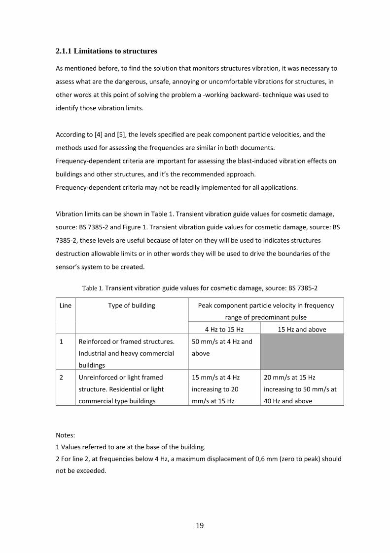
Vibration limits can be shown in Table 1. Transient vibration guide values for cosmetic damage,
source: BS 7385-2 and Figure 1. Transient vibration guide values for cosmetic damage, source: BS
7385-2, these levels are useful because of later on they will be used to indicates structures
destruction allowable limits or in other words they will be used to drive the boundaries of the
sensor’s system to be created.
Table 1. Transient vibration guide values for cosmetic damage, source: BS 7385-2
Line Type of building Peak component particle velocity in frequency
range of predominant pulse
4 Hz to 15 Hz 15 Hz and above
1 Reinforced or framed structures.
Industrial and heavy commercial
buildings
50 mm/s at 4 Hz and
above
2 Unreinforced or light framed
structure. Residential or light
commercial type buildings
15 mm/s at 4 Hz
increasing to 20
mm/s at 15 Hz
20 mm/s at 15 Hz
increasing to 50 mm/s at
40 Hz and above
Notes:
1 Values referred to are at the base of the building.
2 For line 2, at frequencies below 4 Hz, a maximum displacement of 0,6 mm (zero to peak) should
not be exceeded.
20
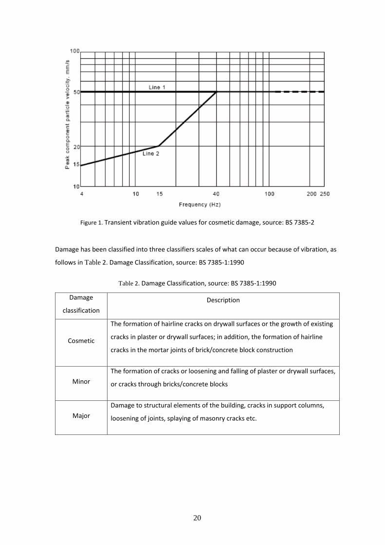
Figure 1. Transient vibration guide values for cosmetic damage, source: BS 7385-2
Damage has been classified into three classifiers scales of what can occur because of vibration, as
follows in Table 2. Damage Classification, source: BS 7385-1:1990
Table 2. Damage Classification, source: BS 7385-1:1990
Damage
classification Description
Cosmetic
The formation of hairline cracks on drywall surfaces or the growth of existing
cracks in plaster or drywall surfaces; in addition, the formation of hairline
cracks in the mortar joints of brick/concrete block construction
Minor The formation of cracks or loosening and falling of plaster or drywall surfaces,
or cracks through bricks/concrete blocks
Major Damage to structural elements of the building, cracks in support columns,
loosening of joints, splaying of masonry cracks etc.

21
According to [3], about describing vibration in the ground and in structures, the motion of a
particle (i.e., a point in or on the ground or structure) is used. The concepts of particle
displacement, velocity, and acceleration are used to describe how the ground or structure
responds to excitation.
Although displacement is generally easier to understand than velocity or acceleration, it is rarely
used to describe ground and structure-borne vibration because most transducers or sensors used
to measure vibration directly measure velocity or acceleration, not displacement.
Accordingly, vibratory motion is commonly described by identifying the peak particle velocity
(PPV) or peak particle acceleration (PPA), for further details, chapters 4, page 13 and 14, as well as
figures 3, 4, and 5 also chapter 6, section 2, page 23: 26 at reference: [3].
Furthermore, According to German Standard [6] Part 3: effects on structures, provides
recommended maximum levels of vibration that reduce the likelihood of building damage caused
by vibration. These levels are ‘safe limits’, up to which no damage due to vibration effects have
been observed for the particular class of building. ‘Damage’ is defined by DIN 4150 to include
even minor non-structural effects such as superficial cracking in cement render, the enlargement
of cracks already present, and the separation of partitions or intermediate walls from load bearing
walls. If such damage is observed without vibration exceeding the ‘safe limits’ it can be attributed
to other causes.

22
Table 3. vibrations effects on structures, source: [6] Part 3
Group Type of structure
Peak vibration velocity, mm/s
Foundation at a frequency Plane of uppermost floor
< 10 Hz 10: 50 Hz 50: 100 Hz All frequencies
1
Buildings used for commercial
purposes, industrial buildings
and buildings of similar design
20 20 to 40 40 to 50 40
2 Dwellings and buildings of
similar design and/or use 5 5 to 15 15 to 20 15
3
Structures that because of
their particular sensitivity to
vibration, do not correspond
to those listed in Lines 1 or 2
and have intrinsic value (e.g.
buildings that are under a
preservation order)
3 2 to 8 8 to 10 8
DIN 4150 also states that when vibrations higher than the ‘safe limits’ are present; it does not necessarily follow that damage will occur.
2.1.2 Sensor selection
Before going through the selection process, there has been a discussion with consultant, about
having an analogue or digital sensor, and a decision has been made that it will be a digital one
because, it’s a lot easier and simpler to merge in electronic circuits, however at the beginning of
searching it has been noticed that analogue sensors are more available and much cheaper, but on
the other hand accuracy and preciseness digital sensors have defiantly won the argument.
As mentioned earlier, vibratory motion is commonly described by identifying the peak particle
velocity (PPV) or peak particle acceleration (PPA), therefore the selection of the sensor has been
narrowed down to sensors that detects velocity or acceleration, luckily acceleration sensors have
what is required; an accelerometer is a sensor which measures the acceleration which it the rate
of change of velocity .

23
According to the available accelerometer sensors in the market there has been a categorisation of
many available accelerometer sensor types the next five are the ones that have been studied:
I. Capacitive MEMS accelerometer
A capacitive MEMS accelerometer sensor detects acceleration with respect to change in
electric capacitance, by the aid of moving diaphragm which act like a moving mass between a
fixed plates, that creates change in capacitance which later on calibrated to show the change
occurred in acceleration to that moving body (diaphragm). MEMS accelerometers are
probably not the most accurate and less noisy signal among all accelerometers, yet it’s the
most available, and easy to use, the reason beyond that probably it’s relatively cheap price
and calibration easiness.
Figure 2. simplified top view of the Analog Devices ADXL50 MEMS sensor a passive, linear accelerometer, source: [8] chapter 7- 7.3.1.14 micromachined IC accelerometer
Linear position of the linear bar proof mass is sensed by 42 pairs of differential capacitive sensing electrodes. A. Accelerometer with zero linear acceleration. B. Accelerometer is accelerating to the right. Source: [8], chapter 7- 7.3.1.14 micromachined IC accelerometer

24
II. Piezoelectric accelerometer
A piezoelectric accelerometer detects changes in acceleration by using piezoelectric effect,
simply by placing a small mass against the axis of measurement, side to side to a piezoelectric
material, which by applying any stress, electric charges produced.
In this case, stress is produced upon the piezoelectric material when the transducer
accelerates. However, the high accuracy and performance of the piezoelectric accelerometer,
the only two disadvantages for this accelerometer first it can be used to measure alternating
acceleration not steady responses, and second it has an expensive price.
Figure 3. piezoelectric accelerometer, source: [9]

25
III. Piezo resistive accelerometer
A piezo resistive accelerometer detects acceleration using a piezo resistive material such as strain
gauge that can reach a range of ±1000 g which makes it very suitable for measuring vibrational
shock events, usually its measuring the change in resistance of piezo resistive material when
acceleration is applied, in the meanwhile the sensor itself is just as expensive as piezoelectric
accelerometer.
Figure 4. piezo resistive accelerometer, source: [9]
IV. Variable inductance accelerometer
A variable inductance accelerometer detects the acceleration just like capacitive accelerometers,
but with the aid of different material, instead of diaphragm a mass of ferromagnetic material is
placed between coil, acceleration is measured as a change in coil inductance when acceleration is
applied, drawbacks are the size of the whole sensor as one can imagine it requires some space for
the mechanical moving parts and as well as wearing of those moving parts.
Figure 5. variable inductance accelerometer, source: [9]

26
V. Hall effect accelerometer
A hall effect accelerometer detects acceleration by the aid of voltage variation resulting from
change in magnetic field which happens by placing a magnet to a moving mass towards/ outwards
a hall element, and same as variable inductance accelerometer the sensor has to be relatively big
in size to carry on all those mechanical parts unlike the MEMS sensor and also worth to mention
how those parts could get worn out after some time.
Figure 6. hall effect accelerometer, source: [9]
From the sense of availability, price, and applicability of accelerometer sensors that can be used
to measure vibration, a capacitive MEMS accelerometer has been chosen for the application out
of all accelerometer sensor types.
Furthermore, capacitive MEMS sensors are digital output sensors, easy to design, don’t need
extra electronic circuitry to operate, only couple of resistors and capacitors in case of I2C or SPI
communication.

27
2.1.3 Sensors comparison
In the market, there were a lot of capacitive MEMS acceleration sensors, with different features
or from different producers, eventually, the sensor to be selected had to have certain features.
According to standards mentioned at section 0], and both drywall graphs which have limitations
of vibration PPV and frequency, and since vibration nature follows the rules of simple harmonic
motion as shown in Figure 7. distance, velocity, and acceleration of simple harmonic oscillation,
source [1].
Figure 7. distance, velocity, and acceleration of simple harmonic oscillation, source [1]
The acceleration range of a vibrational wave required to be measures can be formulated in terms
of velocity and frequency as the following:
𝑥𝑥 = 𝐴𝐴 sin𝜔𝜔𝜔𝜔
At peak: 𝑥𝑥 = 𝐴𝐴
Equation 1.
𝜔𝜔 = 2𝜋𝜋𝜔𝜔
= 2𝜋𝜋𝜋𝜋
Equation 2.
𝑣𝑣 = 𝜔𝜔 𝐴𝐴 sin(𝜔𝜔𝜔𝜔 +
𝜋𝜋2
) At peak: 𝑣𝑣 = 𝜔𝜔𝑥𝑥
Equation 3.

28
𝑎𝑎 = 𝜔𝜔2 𝐴𝐴 sin(𝜔𝜔𝜔𝜔 + 𝜋𝜋)
At peak 𝑎𝑎 = −𝜔𝜔2𝑥𝑥 Assuming positive peak, therefore,
𝑎𝑎 = 𝜔𝜔2𝑥𝑥
Equation 4.
𝑎𝑎 = 𝜔𝜔 (𝜔𝜔𝑥𝑥) = 2𝜋𝜋𝜋𝜋𝑣𝑣
𝑎𝑎 = 2𝜋𝜋𝜋𝜋𝑣𝑣
Equation 5.
𝑣𝑣 = 𝑎𝑎
2𝜋𝜋𝜋𝜋
Equation 6.
Where, x is distance (m),
v is velocity (m/s),
a is acceleration (m/s2),
A is amplitude of oscillation,
ω is angular velocity (rad/s),
f is frequency (Hz or cycle/s), and
t is period of oscillation (s).
Logically, the maximum vibrational event should be detected has to assign the sensor range, and
the minimum vibrational event should assign the sensitivity of sensor to be selected; so, for the
maximum vibrational event should be detected, according to [PPV <100 mm/s, and freq. <100 Hz]
calculated ceiling value is 62,832 m/s2 that means 6,4 g, therefor sensor should have a range of
±80 m/s2 (±8 g) to detect the maximum vibrational magnitude that can affect a building, the
sensor selected has to have at least ± 8 g and can have less configurable range as < ±8, for
example ±2, 4 or 6 g.
For sensitivity whatever the resolution will be, it has to have at least 0,337m/s2/per sensor unit
change at a specific resolution, according to [PPV > 15 mm/s, freq. > 4 HZ]; that means for
example, to detect the least amplitude of vibration wave 0,377 m/s2 sensor should be able to
detect changes at least of 0,337 m/s2, in terms of sensitivity, 1 LSB change for acceleration of
0,337m/s2 at a certain resolution.

29
Most of digital acceleration sensors measures change in acceleration as a unit gravity (g),
1 g = 9,81 m/s2, as well as acceleration sensors sensitivity, mostly it is measured in (sensor
change/mg); some as LSB/g, which is the same as digit/g, and the same as counts/g, these three
are all the same in the sense that they divide the physical acceleration quantity to digital steps as
bits or (counts as one bit is one count).
For that, sensitivity has to follow Table 4. sensitivity with respect to full range in order to detect
the least vibrational wave, which is 0,337m/s2, where sensitivity is less than or equal full range to
least value to be detect
For clarification, one of the sensor’s sensitivity definitions is that the smallest change in output
that can be detected in terms of the full range [8], in this thesis it should be greater than or equal
to the least possible acceleration that could affect a structure as in Equation 7.
sensitivity ≥𝑟𝑟𝑟𝑟𝑟𝑟𝑟𝑟𝑟𝑟𝑟𝑟𝜔𝜔𝑟𝑟𝑟𝑟𝑟𝑟𝜋𝜋𝑟𝑟𝑟𝑟𝑟𝑟 𝑟𝑟𝑎𝑎𝑟𝑟𝑟𝑟𝑟𝑟
�𝐿𝐿𝐿𝐿𝐿𝐿 𝑚𝑚 𝑟𝑟2⁄ �
Equation 7.

30
Table 4. sensitivity with respect to full range
Feature Equation Unit Values
Upper & lower Range - ±g 2 4 6 8
Full range
(2 X upper& lower range)
- 2g 4 8 12 16
1 g = 9,81 m/s2 m/s2 39,24 78,48 117,72 156,96
full resolution (12-bit)
sensitivity
4 096𝜋𝜋𝑟𝑟𝑟𝑟𝑟𝑟 𝑟𝑟𝑎𝑎𝑟𝑟𝑟𝑟𝑟𝑟
𝐿𝐿𝐿𝐿𝐿𝐿𝑚𝑚 𝑟𝑟2⁄ 104,38 52,19 34,79 26,10
Acceleration per one LSB 𝜋𝜋𝑟𝑟𝑟𝑟𝑟𝑟 𝑟𝑟𝑎𝑎𝑟𝑟𝑟𝑟𝑟𝑟
16 384 𝑚𝑚 𝑟𝑟2⁄
𝐿𝐿𝐿𝐿𝐿𝐿
0,0095 0,0191 0,0287 0,0383
full resolution (14-bit)
sensitivity
16 384𝜋𝜋𝑟𝑟𝑟𝑟𝑟𝑟 𝑟𝑟𝑎𝑎𝑟𝑟𝑟𝑟𝑟𝑟
𝐿𝐿𝐿𝐿𝐿𝐿𝑚𝑚 𝑟𝑟2⁄ 417,53 208,77 139,18 104,38
Acceleration per one LSB 𝜋𝜋𝑟𝑟𝑟𝑟𝑟𝑟 𝑟𝑟𝑎𝑎𝑟𝑟𝑟𝑟𝑟𝑟
16 384 𝑚𝑚 𝑟𝑟2⁄
𝐿𝐿𝐿𝐿𝐿𝐿
0,0024 0,00479 0,00719 0,00958
Therefore, the sensor to be selected has to have at least 0,337 m/s2 per unit change, the sensor
selected as shown in tables, Table 4. sensitivity with respect to full range and Table 5. range and
minimum sensitivity, the sensor can reach 0,0024 m/s2/LSB for ± 2 g using 14-bit resolution, which
is way more accurate than needed, and therefore 12-bit resolution has been used in acquisition to
monitor current consumption for the last mentioned resolution, and in the meanwhile to have as
much preciseness as possible.

31
Since the maximum frequency is possible to get out of threating vibration is 100 Hz, according to
Nyquist Shannon theorem, [7] a sufficient sampling rate has to be twice the desired signal to
measured, which means sampling rate has to be at least 200 Hz (sample/second), and according
to sensor datasheet at low power mode, ODR can be 14, 28, 54, 105, 210, 400, 600, 750 [source:
MC3635 sensor’s datasheet P.50 and P.52], an ODR of 200 Hz has been selected as it will have the
least possible current consumption which is 11 𝜇𝜇𝐴𝐴 [source: MC3635 sensor’s datasheet P.18]
𝐿𝐿 < 𝜋𝜋𝑠𝑠 2�
Equation 8.
Where, B signal to be measured (Hz), and
fs is sampling rate (Hz)
Table 5. range and minimum sensitivity
Sensor feature Limit Unit
Range 0,377: 62,832 m/s2
Least value to be detected 0,377 m/s2
Minimum sensitivity at 12-bit resolution for ±2 g 0,0095 (m/s2)/LSB
Minimum ODR 210 Sample/sec
It wasn’t quite easy looking for the right sensor to use, there were a lot of options and a lot of
specifications to go through, on mouser.ee a search was conducted for 3-axis digital MEMS
accelerometer, for that a 123 sensors showed up, all had different ranges, resolution, power
consumption, and other different features; so, search had to narrow down to which of these 123
sensors have evaluation kits, so after so many filtrations only five sensors were able to satisfy
required features, handling all limits, and have evaluation kits.
Those five suitable sensors can be found at table in appendix III

32
2.1.4 Sensor’s uncertainty
Many physical quantities are being measured every day, and according to its purpose and the
organization’s standard these measurements accuracy can vary, for instant measurements for
manufacturing a spaceship are certainly have to be more accurate than measurements for
manufacturing curtains, uncertainty defines the accuracy for the user and the behaviour of any
product under different conditions.
Table 6. Uncertainty calculations from referenced readings at [2.2.4]
Upper magnitude (m/s2) Lower magnitude (m/s2) Peak (𝑥𝑥𝑖𝑖 − �̅�𝑥)2
11,68 -10,03 11,68 6,01
6,79 -13,48 -13,48 18,08
7,37 -2,92 7,37 3,45
7,09 -3,91 7,09 4,57
5,64 -6,79 -6,79 5,95
8,96 -5,59 8,96 0,07
average 9,22
sum 38,13
𝑟𝑟 = �𝑈𝑈𝐴𝐴2 + 𝑈𝑈𝐵𝐵2
Equation 9.
𝑈𝑈𝐴𝐴 = �1
𝑟𝑟(𝑟𝑟 − 1)× �(𝑥𝑥𝑖𝑖 − �̅�𝑥)2
𝑛𝑛
𝑖𝑖=1
Equation 10.
𝑈𝑈𝐴𝐴 = � 16∗5
× 38,13 = 1,271 m/s2

33
𝑈𝑈𝐵𝐵 = �𝑈𝑈𝑠𝑠𝑠𝑠2 + 𝑈𝑈𝑅𝑅𝑅𝑅𝑅𝑅2 + 𝑈𝑈𝑅𝑅𝑅𝑅𝑅𝑅2 + 𝑈𝑈𝑀𝑀𝑅𝑅𝑀𝑀2 + 𝑈𝑈𝑅𝑅𝐸𝐸𝐸𝐸2
Equation 11.
Data are found for 𝑈𝑈𝑅𝑅𝑅𝑅𝑅𝑅 and 𝑈𝑈𝑅𝑅𝑅𝑅𝑅𝑅 only therefore,
𝑈𝑈𝐵𝐵 = �𝑈𝑈𝑅𝑅𝑅𝑅𝑅𝑅2 + 𝑈𝑈𝑅𝑅𝑅𝑅𝑅𝑅2
Equation 12.
𝑈𝑈𝑅𝑅𝑅𝑅𝑅𝑅 = 𝑈𝑈𝑎𝑎
Equation 13.
𝑈𝑈𝑅𝑅𝑅𝑅𝑅𝑅 =1,271 m/s2, since values quantity is more than five
𝑈𝑈𝑅𝑅𝑅𝑅𝑅𝑅 =𝑟𝑟𝑠𝑠𝑎𝑎𝑟𝑟𝑟𝑟 𝑟𝑟
2√3
Equation 14.
𝑈𝑈𝑅𝑅𝑅𝑅𝑅𝑅 = ±22√3
= 22√3
= 0,57 m/s2, since digital sensor.
𝑈𝑈𝐵𝐵 = �(1,271)2 + (0,57)2 = �1,615 + 0,33 = 1,39 m/s2
𝑟𝑟 = �1,2712 + 1,392 = �1,615 + 1,93 = 1,88 m/ss
expanded uncertainty, where K is constant and equals to 2
𝑈𝑈 = 𝑘𝑘.𝑟𝑟
Equation 15.
𝑈𝑈 = 2 × 1,88 = 3,76 m/s2
Therefore, the sensor uncertainty is ± 3,76 m/s2 when using ± 2 g range

34
2.1.5 Communications
Communication with and on the device are two separate parts inter and external
communications, in both stations the first of trial using the Arduino alike board (badger board)
and on the actual product to be manufactured.
For the development purpose, internal communication is the communication carrying the data
out of the sensor to the development board and the external one is the communication that carry
the data processed on the development board (badger board) to the logging board (raspberry-pi).
For the production purpose, the internal communication is the same, but the external
communication is the one that differ than the development phase, in the sense that instead of
communicating with a logger board, it’s communicating and sending data to LoRaWAN gateway.
Internal communication has been using SPI, to send data from sensor to development board
(badger board), because of two main reasons SPI has been chosen over I2C, first is that SPI has
higher data transmission rate, second is that SPI doesn’t need extra circuitry such as pull-up or
pull-down resistors, with 2 Mbps data rate which has been chosen to operate SPI communication,
so that current consumption would be minimized, the sensor itself can operate on SPI data rate
up to 8 Mbps, and maximum power consumption would be 10 µA [source: MC3635 sensor’s
datasheet]; Same data transmission rate of SPI will be used for production as it’s sufficient from
the points of view of data acquisition and power consumption.
For research and development purposes, serial communication has been chosen to send raw data
from development board (badger board) to logging development board (raspberry-pi), using
sensor’s ODR of 210 Hz, the data has been sent over serial communication using baud rate of
9600 to be logged as will be mentioned at subsection [0]

35
2.2 Implementation
As mentioned previously, the aspects that matter the most to monitor structures vibration, the
three main aspects that affect structures health or safety [1.4.1],
first vibration amplitude, second total time of vibration, third the frequency of the vibration
however it’s a shock vibration, or a continuous vibrational wave, also as discussed earlier, the
selected sensor measures acceleration, and since vibration in nature is a wave therefore it has
acceleration and velocity as well as a propagational distance.
However, acceleration is an important component of vibration so it can drive velocity peaks with
the knowledge of other parameters, yet customers won’t get any benefit out of only its raw
acquired values (acceleration)!
Indeed what matter most for customers the three aspects that affect buildings safety standards
stated by concerned departments or authorities with a time stamp for vibrational event
occurrence for structures owners so that it can be used to warn surrounding vibration sources or
responsible for it; or construction sites to monitor and maintain their produced vibration, which
can be handled by LoRaWAN, as it has relatively small bandwidth.
For that data acquired and logged has been analysed to show those vibrational event aspects so,
the peak is easy to get as it’s the maximum value(s) of the vibrational event, however the total
time of event can be a bit tricky to estimate, as its mainly defined by the definition of what are the
limits that are considered dangerous or should be counted, moreover the frequency calculation,
for that or in order to get a reliable frequency calculation, a good samples and sample rate have
to be considered, or taken into account as the more defined the signal of vibrational wave, the
more Its analysis will be framed more efficiently.

36
2.2.1 Data acquisition
To acquire vibration samples that can be analysed, a simple acquisition device has been made to
simulate the device to be produced. A container that contains a power bank, development board
(raspberry-pi) act as a small computer logs and supply other peripherals, another development
board (badger-board manufactured by NAS and schematically similar to Arduino LilyPad) that acts
like an acquisition controller and an accelerometer (the selected acquisition sensor).
Data acquisition has been carried out at three different structures, located at three different
vibration noise;
a. NAS office, a quite newly constructed, and well reinforced building (at Haabersti district o
in Vabaõhumuuseumi/ Paldiski streets)
b. A modern house 50 m away from a construction site (at Lasnamäe district in Uuslinna
street)
c. A 70 years old house next to a heavy traffic main road (at Kesklinn district in Endla street)
Luckily the three structures have given the opportunity to test the applicability of different
scenarios of vibration, acquisition at the first and the last were indoor while the on the second
structure device was operating in a balcony in front of the construction site.
For information, while the sensor acquisitions the temperature, and humidity were being
monitored, as that any sensor exists have temperature response and drift, which was taken in
consideration.

37
2.2.1.1 First misconnection error
While the first attempt to get output data out of the sensor, a first step to make sure all
connections of evaluation kit were correct and sensor is working as datasheet specification claims,
no reading came out of the sensor through serial bus, there were no response at all!
As the debugging begun, it was needed to make sure that all connections were connected as
mentioned in the datasheet of the evaluation kit, with the aid of multi-meter a continuity check
has been conducted to make sure wires are fine, so next step of debugging was to make sure the
sensor itself is fine, therefore an oscilloscope has been connected to sensor’s SCLK, MOSI and
MISO pins of the SPI connection to check that they are either receiving the right input or
transmitting the correct output, at this debugging point the test conducted showed strange
behaviour!
Serial clock, MOSI and MISO signals were totally missed up, as shown in Figure 8. sensor’s SPI
MOSI signal, source: oscilloscope output and Figure 9. sensor’s serial clock signal, source:
oscilloscope output.
Figure 8. sensor’s SPI MOSI signal, source: oscilloscope output

38
Figure 9. sensor’s serial clock signal, source: oscilloscope output
Those oscilloscope measurements had aroused two doubts one about the connection’s validity
and the other about the faultiness of the whole sensor, by checking the connections once again, a
faulty jumper wire on the VDD (supply voltage) has been discovered this time, the wire itself was
good but it’s jumper holding on the sensor’s pin header (from sensor’s side not development
board) was faulty, as shown in Figure 10. jumper wire connection error, source: google images,
the red circle shows exactly where the fault was.
Figure 10. jumper wire connection error, source: google images
By changing that faulty jumper wire, the sensor responded normally as mentioned in the
datasheet, and readings are found in data analysis subsection [0].

39
2.2.2 Data logging
Mainly the combination above had to collect data with different parameters settings, in the sense
that highly accurate data would be useful as much as the data with minimum signal definitions
(least resolution, least acquisition data rate), in this way there will be a better understanding of
how what is the best suitable waking and sleeping data rates and other features to be defined.
The simulating device mentioned above, was configured as the following, the sensor connected to
the badger-board through SPI connection, where the badger-board was polling and controlling
the acceleration measurements of the sensor library when an interrupt pin is set high from the
sensor which indicates a new fresh measurement is ready and then request another one from the
sensor; the badger-board connected to the raspberry-pi through a USB port where the badger-
board sends the acquired measurements for the three axis X, Y, and Z through serial
communication and the raspberry-pi reading these measurements and logging them into CSV files
along with a timestamp; and finally the raspberry-pi connected to a power bank or an AC adapter
depends on either there’s a power source nearby or not, or is it indoor or outdoor.
Figure 11. sensor container schematic, source: created via draw.io

40
Figure 12. acquisition program flow chart, source: created via draw.io

41
2.2.3 Data analysis and manipulation
There were two implementations of data analysis for the data acquired, the first was at testing
the sensor and its output data, the second was the real implementation occur inside MCU just
before sending network packets.
At first as a research about sensor capabilities and current consumption, data arrays of
acceleration and timestamp has been logged into CSV files, then many mathematical operations
have been applied to these sets of data to determine the parameters that matters the most when
comes to vibration analysis.
Then second, because of the importance of further calculations over the raw data acquired from
the sensor as mentioned before, just after logging the acceleration data, some of those previously
tried out mathematical operations have been applied to these arrays of data for each axis, so that
it finally can sends them as LoRa packets which will be visualised over the server.
For instant the analysis of vibrational events can calculate, i.e. FFT for these vibration frequency
components, or PPV, or total duration of vibration; these parameters are the data that
determines all what is necessary to know about the vibrational event occurred, and moreover
what matter the most to customers.
Data acquired were constructed as the following CSV line:
2019-03-23 20:14:35, 1.67, -0.89, -9.91
Representations:
Table 7. sensor output line example
Timestamp
YYYY-MM-DD hh:mm:ss
X acceleration
(m/s2)
Y acceleration
(m/s2)
Z acceleration
(m/s2)
2019-03-23 20:14:35 1.67 -0.89 -9.91

42
Because of the sensor selected has three operating modes, precision, low power, and ultra-low
power, as a first trial of sensor, data acquired at low power mode to check how’s medium level
acquisition noise and accuracy, ODR was first selected to be 105 Hz, using the output of interrupt
pin, an oscilloscope of a KEYSIGHT 34465A 61/2 DMM was connected to measure the ODR, which
had an average of 105,0018 Hz for the first 5 k samples, just similar to what was mentioned at the
datasheet (page 52/84), and that can be shown in Figure 13. sensor ODR of 105 Hz (1), source:
DMM output.
Figure 13. sensor ODR of 105 Hz (1), source: DMM output
However, at 16 k samples the average started to deviate a little, to give out ODR of value
104,282 HZ, still the ODR was not bad, almost 99% accurate to what the datasheet range has
proclaimed, Figure 14. sensor ODR at 105 Hz (2), source: DMM output.
Figure 14. sensor ODR at 105 Hz (2), source: DMM output

43
Then another set of data acquired for almost 2,5 minutes, exactly 155,9 seconds of total 32,74 k
samples using only ± 2 g range with using ODR of 210 Hz, Figure 15. three axes 32,74 k sensor
samples, source: python analysis script, indicates how different hits on a disk holding the sensor
are shown for axes X, Y and Z, also the gravity victor can be shown on y-axis as a down-shift of
-10 m/s2.
Also it’s clear that for some vibrations the range limit of ± 20 m/s2 is not enough even though the
simple hits on the disk the range was not enough, imagine more vibrational events produced by
construction sites using high vibrational equipment like jack-hammer, or heavy traffic road, it was
obvious that the range was selected from the calculations of ± 8 g makes more sense, and that
exact point a decision has been made to acquire the rest of sample using ± 8 g.
Figure 15. three axes 32,74 k sensor samples, source: python analysis script

44
To asses one vibrational event, a signal has been filtered out, of 300 samples in the range of
31000: 31300, for the three axes as can be shown in Figure 16. 300 samples extracted out, source:
python analysis script, where each row indicates an axis, on the left vibrations signal from the
sensor, on the right FFT of the graphs on the left, it’s clear for the Y-axis which was parallel to the
desk surface FFT corresponding graph has a frequency of 20 seconds which was as calculated
24 Hz.
A sample has been evaluated at Figure 16. 300 samples extracted out, source: python analysis
script, as shown, PPA was 11 m/s2, and according to Equation 6., 𝑣𝑣 = 𝑎𝑎2𝜋𝜋𝜋𝜋
= 112×𝜋𝜋×24
=
0,072𝑚𝑚 𝑟𝑟⁄ = 72 𝑚𝑚𝑚𝑚/𝑟𝑟
Figure 16. 300 samples extracted out, source: python analysis script

45
To decide which events analysis method to use, samples of data acquired can be visualised as
shown in Figure 16. 300 samples extracted out, source: python analysis script, Figure 17. 14 k
sensor samples, source: python analysis script, for 70 seconds
a 14 k sample were taken with various shock on the desk, by only visualising the parallel axis (Y) to
the desk surface.
Figure 17. 14 k sensor samples, source: python analysis script

46
One of the proposed analysing approaches to sample the wave was to cut it into samples of 100
that gave 14 trimmed samples (raw data on the left) and (FFT is given on the right) shown in
Figure 18. samples of 100 first, source: python analysis script, and Figure 19. samples of 100
second, source: python analysis script.
Figure 18. samples of 100 first, source: python analysis script

47
Figure 19. samples of 100 second, source: python analysis script

48
Another approach was to cut of each event separately which, and that approach was richer in
data as shown in Figure 20. vibrational events of the 14 k samples, source: python analysis script,
only vibrational events for the given sample event, then analysis each event separately, so that a
better understanding of each event independently.
Figure 20. vibrational events of the 14 k samples, source: python analysis script

49
2.2.4 Acquired data referencing
A reference has been used to verify that the output data of the sensor are close as possible to the
ideal output, for the first glance it might be not so convenient reference, but it has shown almost
similar acceleration, considering the difference in sensors containers and how they are fixed and
exposed to vibration, such deviation makes sense to appear in readings.
An iPhone 7 accelerometer was used to verify that the sensor is operating as the features in its
datasheet has proclaimed, by the help of an application called VibSensor, the vibration acting
upon the three axes X, Y, and Z was calibrated as intended, the gravity vector has been eliminated
from the sensor output, and only the vibration was visualized to verify the sensor output.
Figure 21. VibSensor referenced acquired data, source: VibSensor mobile app

50
Figure 22. VibSensor referenced acquired data analysed using python script, source: python analysis script
As shown in Figure 21. VibSensor referenced acquired data, source: VibSensor mobile app, Figure
22. VibSensor referenced acquired data analysed using python script, source: python analysis
script and Figure 23. sensor’s data acquired to be referenced, source: python analysis script, data
acquired from both the sensor and the mobile application are almost identical, however both
readings are in different measuring units (m/s2 and g respectively) it’s obvious from the graph that
Z-axis in both has the highest vibration shocks, and for that small deviation an uncertainty
calculations has been conducted at [2.1.4].
N.B. in Figure 22. VibSensor referenced acquired data analysed using python script, source: python analysis script and Figure 23. sensor’s data acquired to be referenced, source: python analysis script, the three axes vibration is a combination of the three axes together, blue: x-axis, orange: y-axis, green: z-axis.

51
Despite that the graphs looks identical, the actual numbers were slightly deviated, for example in
the mobile application the peak 12.66 m/s2, but from the sensor 11.84 m/s2, for that to make sure
another vibration reference was needed, just to make sure that the sensor’s readings are within
allowable range.
Figure 23. sensor’s data acquired to be referenced, source: python analysis script

52
2.2.5 Power consumption management
One great advantage of the ultra-low power vibration sensor that, it’s intended to be a
standalone IoT node.
As mentioned before at the very first section, current available method is human dependant,
which means human error, that doesn’t mean that the solution offered doesn’t has human errors!
It’s limited as much as possible though; that means only human error exists while first fixing the
device, however a simple container design can assure that fixing the device has proper physical
contact with “a surface” the device has a calibration to smartly know where the earth’s gravity is
pointing, please notice that the quoted word, it’s needed to have a physical contact with any
ground or wall, or any surface fixed to the structure.
For that and for the other technologies in use like a LoRaWAN the device, and in general how
most of products being designed at NAS are battery powered, therefore the whole device has to
operate at low power as it can detect the vibration affecting structures, however frequency,
magnitude of vibration etc.; running the device with full definitions (resolution, maximum amount
IoT packets etc.) will drain the battery quickly which is not convenient for neither product R&D
nor customers, it’s better with sense to have the device the longest time possible.
Keeping that previous rule beard in mind will set a good, and reliable approach of design; for that
to be achieved, device has to have for instance to sniff if there’s acceleration change within some
threshold level, with the lowest power consumption; and moreover how to smartly tune itself so
that it can get the most accurate data relative to the lowest power consumption.
And eventually sends a network packet of data contains just the important data for the customer.
Current drawn at somehow high precise acquisition mode was nearly 0,108 mA at development,
for all of the following: raspberry-pi, badger board, sensor at the following conditions: sensor’s
ODR of 210 Hz, 12-bit resolution, a range of ± 8 g (however acquired data was in the range of +20
and -50 m/s2 or in g unit +2 and -5 g) and operating power mode “low power mode”, by
transmitting data over SPI with data rate of 2 Mbps to badger board, and the badger board
transmitting the acquired raw acceleration data over serial bus with baud rate of 9600 to
raspberry-pi board so that it logs them to CSV file along with the timestamp of the acquisition.

53
The typical battery life with considering worst RF transmission, weather conditions etc. is equal
to, 𝐿𝐿𝑎𝑎𝜔𝜔𝜔𝜔𝑟𝑟𝑟𝑟𝐵𝐵 𝑟𝑟𝑟𝑟𝜋𝜋𝑟𝑟 = 𝐵𝐵𝑎𝑎𝑠𝑠𝑠𝑠𝐵𝐵𝐵𝐵𝐵𝐵 𝑐𝑐𝑎𝑎𝑐𝑐𝑎𝑎𝑐𝑐𝑖𝑖𝑠𝑠𝐵𝐵 (𝑚𝑚𝐴𝐴ℎ)𝑙𝑙𝑙𝑙𝑎𝑎𝑙𝑙 𝑐𝑐𝑐𝑐𝐵𝐵𝐵𝐵𝐵𝐵𝑛𝑛𝑠𝑠 (𝑚𝑚𝐴𝐴)
.
For the following assumptions the battery life time has been calculated:
Table 8. approximation of current consumption
Peripherals Sleeping Current consumption (mA) Waking Current consumption (mA)
MCU 0,001 100
LoRaWAN RF 0 0,00288
Sensor 0,015 0,015
Total 0,0115 100,01788
Figure 24. LoRaWAN power consumption estimation, source: calculated

54
From Table 8. approximation of current consumption and Figure 24. LoRaWAN power
consumption estimation, source: calculated, and assuming that for all day long sensor is operating
in sniffing mode which is powered with ultra-low power consumption, that consumes 0,0038 mA,
for 3 times a day a packet will be sent and that consumes 300,01788 mA, and it lasts about 30
seconds to send the packet of analysed data as mentioned before and acknowledge it, then the
device goes back to sniffing mode to reduce power consumption.
If battery is 2700 mAh, therefore at sleeping mode, battery life is 234782,609 hours = 26,8 years
And at waking mode is 8,999 hours.
Since the sensor will send packets 3 times a day, therefore working capacity while waking
is 𝐶𝐶𝑤𝑤 = 𝐼𝐼 × 𝑇𝑇, while (Cw) is awoke capacity, (I) is current consumption, (T) is running time,
(CS is sleeping capacity).
Therefore 3 minutes will be Cw= 2,5 mAh per one day
And at sleeping mode CS = 0,276 mAh per one day
Therefore, battery life is almost 2,66 years or 972,62 days for mentioned conditions and
assumptions of surroundings and rated usage current consumption.
N.B. all previous calculations were calculated upon worst conditions

55
2.3 Success measurement
The thesis, or research success could be determined upon:
- how precise the sensor will be compared to its power consumption,
- how sensitive it is for ground smallest vibrations,
- how good are the static and dynamic characteristics of the sensor, time is considered to
be one of the critical factors that the sensor should handle?
- How far better sensor is compared to other solutions?
The success of thesis is the answer of all these previously -how questions- are answered, and how
consistent were the steps taken to figure it out.
2.4 Data acquisition, code and sensor library manipulation
For data acquisition, there were two codes needed one for both the DAQ, which is Arduino/C++
code based, and one for the logger board which is python based.
Luckily the sensor used has a library constructed by the sensor’s manufacturer, which maps all
registers needed to control all sensor’s aspects, it has been used to send a struct of C++ data of
acceleration in the three dimensions X, Y, and Z and surrounding temperature over serial bus,
from the other side of that serial bus awaits the raspberry-pi board to log those acceleration
results and temperature, with a simple python code will go through it later on.
DAQ board code that polls the data out of the sensor can be found at Appendix I
Logging code can be found at Appendix II

56
3 RESULTS
This section will cover all answers of all questions have been asked through the whole paper as a
problem-solving method, define some problem, ask questions to find ways to solve it, find some
solutions and sort them by efficiency after researching about them, and trying some of them if
possible.
what is the nature of vibrations threating structures?
As observed in research, vibration can be in form of continuous noise or separate events of
shocks, depends on the source producing the vibrational event, for example jackhammer
producing continuous vibration or a heavy item dropped on the ground or a heavy truck passing
by the structure being monitored, in both cases velocity and frequency of the vibration are what
matter the most for estimating danger level to the structure.
what are the solutions/ technologies that the market can provide?
As mentioned before, there are consultations construction companies that offers monitoring
vibrations for structures by fixing vibrations sensing probes to estimate if there is any vibration
and is it danger or not, they offer their services to any house owner suspects of vibration danger
on their house, the solution is working, yet so expensive and can have high human error, since
eventually humans are fixing those probes anyway.
There are other technologies which are offering vibration sensing devices that can estimate
vibration characteristics, yet their services are only limited to high frequency vibration sources like
factories machinery, so that maintenance can be carried properly and predictive maintenance can
be assured using the aid of highly accurate sensors, good solution for machinery vibrations
monitoring, but for structures which vibration limits and fear standards are totally different, in the
sense that they are much less in velocity and frequency, such devices won’t be the right choice
(highly overrated) to assess vibrations acting on structures.
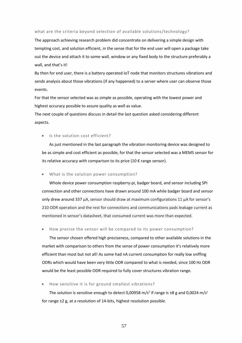
57
what are the criteria beyond selection of available solutions/technology?
The approach achieving research problem did concentrate on delivering a simple design with
tempting cost, and solution efficient, in the sense that for the end user will open a package take
out the device and attach it to some wall, window or any fixed body to the structure preferably a
wall, and that’s it!
By then for end user, there is a battery operated IoT node that monitors structures vibrations and
sends analysis about those vibrations (if any happened) to a server where user can observe those
events.
For that the sensor selected was as simple as possible, operating with the lowest power and
highest accuracy possible to assure quality as well as value.
The next couple of questions discuss in detail the last question asked considering different
aspects.
• Is the solution cost efficient?
As just mentioned in the last paragraph the vibration monitoring device was designed to
be as simple and cost efficient as possible, for that the sensor selected was a MEMS sensor for
its relative accuracy with comparison to its price (10 € range sensor).
• What is the solution power consumption?
Whole device power consumption raspberry-pi, badger board, and sensor including SPI
connection and other connections have drawn around 100 mA while badger board and sensor
only drew around 337 μA, sensor should draw at maximum configurations 11 μA for sensor’s
210 ODR operation and the rest for connections and communications pads leakage current as
mentioned in sensor’s datasheet, that consumed current was more than expected.
• How precise the sensor will be compared to its power consumption?
The sensor chosen offered high preciseness, compared to other available solutions in the
market with comparison to others from the sense of power consumption it’s relatively more
efficient than most but not all! As some had nA current consumption for really low sniffing
ODRs which would have been very little ODR compared to what is needed, since 100 Hz ODR
would be the least possible ODR required to fully cover structures vibration range.
• How sensitive it is for ground smallest vibrations?
The solution is sensitive enough to detect 0,00958 m/s2 if range is ±8 g and 0,0024 m/ss
for range ±2 g, at a resolution of 14-bits, highest resolution possible.

58
• Does the solution cover all important parameters of structures vibrations, so that it can be used later for vibrational evaluation?
Using some statistical computations, that by knowing raw data their amount and
acquisition rate it’s possible to compute FFT and vibration peak velocities, which is all
necessary to analyse vibration of any structure.
• Is this solution efficient in general?
Yes, the solution is capable of evaluating structures vibrations, and more importantly its
accurate, however the current consumed while testing the device was more than expected.
• What were the results with comparison to what has been initially asked, how good is it possible to achieve a device monitoring structure vibration?
The solution is not the best because of sensor’s high current consumption, however with
more manipulation of the sensor’s library and its features, better current consumption could
be achieved, for example by using another combination of features like, less range, less
resolution, and another operating mode like ULP.
• How far better is the sensor, compared to other solutions?
Comparing the sensor as a solution, it would be better from the sense that it’s simpler
and as accurate as other solutions being offered in the market however it didn’t prove better
power performance, so from one side it’s already better, and another it needs more
development.
• How good are the static and dynamic characteristics of the sensor, time is considered to be one of the crucial elements that the sensor should handle?
Static characteristics of a sensor are the features that are almost constant or slowly
varying with time, such as accuracy, precision, sensitivity, linearity, repeatability, drift,
resolution, dynamic characteristics of a sensor are the features that are changing with time,
such as response time, dynamic error.
The sensor itself had very stable static and dynamic characteristics and has given stable
measurements though testing, readings were consistent and within the datasheet margin
ranges of errors.

59
4 DISCUSSION
As seen from results, that the sensor is accurate and precise it have detected fine acceleration
changes in other words it have detected small vibrations, however the current consumption was
not as small as predicted still its configurations can be tuned to have less resolution and range so
it would consume less power.
As an overall solution it’s more practical than current solutions available in the market since it
doesn’t need any highly skilled human interaction to be fixed or to interpret readings, they are
tested and verified, only the device has to be fixed against some wall in the structure and that’s it.
About protocols and technologies used to achieve the solution, they were selected to keep the
solution as simple as possible, as well as having the least power consumption possible, and the
most cost efficient choices, for example using more accurate sensor as piezo electric sensor,
would have given more accurate measurements however its high price (+1000 €), eventually it
would be really expensive and accurate IoT node, but using a MEMS sensor on the other hand has
given relatively great results compared to its reasonable market price, it has satisfied the needs
for monitoring structure vibrations.
Also to mention, LoRaWAN technology has been always a good solution for IoT because of the
high secure connection, [NAS website] pi-directional communication which reduces the need for
expensive man hours, and low power consumption which customer preferable, and long range of
service, using some antennas it can reach a coverage of more than 90 km.

60
5 CONCLUSION
As a final conclusion of the solution and it’s achieved results, monitoring structures vibrations
through ultra-low power IoT node is simple, accurate, and possible to implement.
Although achieving ultra-low power consumption in this approach has been critical because of
many sensor’s features to tune and the electronic pads current leakage.
Structures vibrations can be monitored through ultra-low power accelerometers, that have at
least sensitivity of 0,377 m/s2, and range up to ±8 g.

61
SUMMARY
In order to keep buildings or structures in general safe from vibrations that happens due to
construction work or heavy road next to buildings, as well as keep monitoring structures that have
to stay in range of least vibration such as hospitals and historical buildings, a solution that can
monitor vibrations with good accuracy was needed using ultra-low power consumption so that it
can fit in IoT LoRaWAN family and can be reliable, cost efficient, and has high precision.
There already solutions exists on the market that have been reaching out the same problems, like
a consultation companies that offer a service of monitoring vibration sensing devices around house
and calculate structures vibration, the solution is efficient technically, it’s observable that it might
have some technical errors due to human interaction, in the mean while the solution is offered
here is out of the box, just attach the sensor to some wall and its ready to monitor structures
vibrations, plus its much cheaper than the service being provided by consultants, yes it might be
less detailed but it has every important aspect house owners or construction sites engineers might
need, with no extra data might be irrelevant, and if needed any extra parameters can be calculated
if customer requested from company.
After researching about the limits that the standards have declared for structures vibrations, PPV
or frequency, and by having raw data of acceleration, it’s acquisition time and rate it was easy to
calculate vibrations PPV and frequencies through FFT and simple harmonic motion equations, so
the device can monitor vibration and provide data about its features like the two mentioned before
(PPV and frequency of vibrations) and that is what customer might need to evaluate any vibrational
event can affect structures.
For that a sensor had to be chosen to satisfy device criteria of accuracy, range, sensitivity and
ultra-low power consumption, among the sensors and technology a sensor has to have more
convenient price to performance ratio, overall they have to match certain limits and selection
criteria, an accelerometer found to be one of the most efficient raw data to be used to calculate all
necessary parameters that can monitor structures vibrations such as frequency and PPV,
acceleration can be used to measure vibrations and their characteristics by the aid of simple
calculations of acceleration rate and magnitude.

62
After searching for a suitable sensor, a MEMS accelerometer has been chosen that had all required
features, and upon first trial there were no reading, hence debugging took place to figure out the
problem, and after some trials, it has been found out that the jumper wire connecting the sensor
and the acquisition board (badger board) was faulty and didn’t connect terminals properly, as soon
as it got changed, it gave acceleration readings out through SPI bus and the issue has been solved.
However, the high accuracy the sensor has delivered there are doubts about its power
consumption, and for that it considered to look for better configuration in the future as
development of the product, so that better power consumption would be achieved.
Furthermore, sensor’s Arduino library should be transformed to a C or C++ library so that it can fit
with the company’s SDK, and for that packing shall be used to transform it.
As a result of technologies selected to solve the problem and to approach a reliable solution that
meets the problem effectively, a precise system has been built to analyse and evaluate vibrations
that can affect structures health or their lifetime, for testing along with a MEMS accelerometer, an
acquisition development board (a badger board) that receive raw data from accelerometer and
extract data with the specified ODR and logging board (raspberry-pi) that log data sent from the
first development board through serial bus, compute its FFT and PPV, for actual implementation
there will be no logging board but instead data will be analysed inside MCU and sent through
LoRaWAN whenever off-range vibrational event happens.
As a personal opinion, the achieved device is simple, out of the box solution, precise, and cost
efficient, however, there must be some future development concerning power consumption, as a
final product it could be in price range of 25: 30 €, comparing it to other solution available in the
market its way more cheaper, can be used by house owners, construction sites, hospitals, historical
buildings to monitor vibration affecting structures or exerted by construction work or if it has been
taken for further development, it can be used to evaluate machinery vibrations in industrial plants.

63
LIST OF REFERENCES
[1] William T. Thomson & Marie Dillon Dahleh, Theory of vibration with applications,
Prentice Hall, fifth edition, 1998
[2] Singiresu S. Rao, Mechanical vibrations, Addison-Wesley, third edition, 1995
[3] Jim Andrews, David Buehler, Harjodh Gill, Wesley L. Bender, California Transportation
and Construction Vibration Guidance Manual, September 2013
[4] BS 7385-1:1993, BS 7385-2:1993 Evaluation and measurement for vibration in buildings
[5] Guide to damage levels from ground borne vibration and the United States Bureau of
Mines (USBM) RI 8507 Impacts to structures
[6] DIN 4150–3:1999–02 Vibration in buildings
[7] Robert J. Marks II, introduction to Shannon sampling and interpolation theorem,
Springer, 1991
[8] Robert B. Northrop, Introduction to Instrumentation and Measurements, Tylor & Francis,
second edition, 2005
[9] Accelerometers types: https://www.engineersgarage.com/articles/accelerometer

64
APPENDICES
Appendix I */Arduino Main code, there are other libraries all project can be found on …*/
//include libraries
#include "MC3635.h"
#include "badger.h"
//define variables and constants
unsigned long c = 0;
int old_XAxis = 0; int old_YAxis = 0; int old_ZAxis = 0;
const byte interruptPin = 2;
const int idx = 0;
volatile bool x = 0;
uint32_t mil = 0;
uint32_t old_mil = 0;
uint8_t counter = 0;
//initialise sensor class
MC3635 MC3635_acc = MC3635();
void setup() {
Serial.begin(9600);
delay(5000);
pinMode(interruptPin, INPUT);//INPUT_PULLUP);
attachInterrupt(digitalPinToInterrupt(interruptPin), read_sensor, RISING);
MC3635_acc.Enable_interrupt(idx);
MC3635_acc.SetNumOfDevice(1);
MC3635_acc.SetCSPin(idx, 11);
MC3635_acc.SetInterface(1);
MC3635_acc.start(1); // SPI interface
badger_init();
}
void loop() {
if (x == 1)
{

65
write_acc_only();
}
}
void read_sensor () {
x = 1;
}
void write_acc_only (){
mil = badger_millis ();
if (mil-old_mil >= 4000) {
get_temp_hum ();
old_mil = mil;
}
else {
MC3635_acc_t rawAccel = MC3635_acc.readRawAccel (idx);
Serial.print(rawAccel.XAxis); Serial.print(","); Serial.print(rawAccel.YAxis); Serial.print(",");
Serial.println(rawAccel.ZAxis);
x = 0;
MC3635_acc.clear_int(idx);
}
}
void get_temp_hum(){
int result[4];
int *res_pointer = result;
x = 0;
MC3635_acc_t rawAccel = MC3635_acc.readRawAccel(idx);
MC3635_acc.clear_int(idx);
badger_temp_sensor_send(res_pointer);
Serial.print(rawAccel.XAxis); Serial.print(","); Serial.print(rawAccel.YAxis); Serial.print(",");
Serial.print(rawAccel.ZAxis); Serial.print(",");
Serial.print(result[0]); Serial.print("."); Serial.print(result[1]); Serial.print(","); Serial.print(result[2]);
Serial.print("."); Serial.println(result[3]);
}

66
Appendix II
# import libraries
import os
import numpy as np
import math
import matplotlib.pyplot as plt
from scipy.fftpack import fft
from statistics import mean, stdev, median, pstdev
class AnalyseVibration(object):
# initialisations and constants
pi_log_root = "./log/pi_logs/"
test_log = "./log/test_log/"
pc_log_root = "./log/raw/"
log_history = "./log/log_history/"
test_log_dist = "./log/test_log_dist/"
ref_log = "./log/ref/"
curr_log = "./log/curr_cons/"
working_dir = curr_log #pc_log_root
#res = "./results_15_03_19.csv"
start_x = 'X'
start_y = 'Y'
start_z = 'Z'
x = []
y = []
z = []
component = []
total_amount = 0
N = 0
Fs_old = 50
Fs = 210
t = 0.0025

67
def __init__(self):
self.append_dir_content()
self.show_plot()
#self.disc_samples()
#self.peaks_samples()
# read lines in file
def open_file(self, file_path):
with open(file_path, "r") as f:
file_content = f.readlines()
f.close()
return file_content
def get_data_amount(self):
self.total_amount = len(self.x)
if self.total_amount <= 10000:
amt_roun = round(self.total_amount, 2)
return amt_roun, ""
elif (self.total_amount > 10000) and (self.total_amount <= 1000000):
amt_roun = round(self.total_amount/1000, 2)
return amt_roun, "K"
elif self.total_amount > 1000000:
amt_roun = round(self.total_amount/1000000, 2)
return amt_roun, "M"
def cut_plot(self):
range_low, range_up = 20000, 40000
self.x = self.x[range_low:range_up]
self.y = self.y[range_low:range_up]
self.z = self.z[range_low:range_up]
self.component = self.component[range_low:range_up]

68
self.N = len(self.x)
def show_plot(self):
#self.cut_plot()
#plot = self.get_fft()
#plot = self.the_other_get_fft()
self.remove_gravity()
amt_of_x = self.get_data_amount()
fig = plt.figure()
dt =1
t = np.arange(0, self.N, dt)
'''ax1 = fig.add_subplot(4, 2, 1)
ax2 = fig.add_subplot(4, 2, 3)
ax3 = fig.add_subplot(4, 2, 5)
ax_com = fig.add_subplot(4, 1, 4)'''
ax1 = fig.add_subplot(5, 1, 1)
ax2 = fig.add_subplot(5, 1, 2)
ax3 = fig.add_subplot(5, 1, 3)
ax_total = fig.add_subplot(5, 1, 4)
ax_com = fig.add_subplot(5, 1, 5)
'''ax4 = fig.add_subplot(4, 2, 2)
ax5 = fig.add_subplot(4, 2, 4)
ax6 = fig.add_subplot(4, 2, 6)'''
ax1.set_ylim(-20.1, 20.1)
ax1.plot(self.x)
#title = 'vibration of {0}{1} samples in range of '.format(amt_of_x[0], amt_of_x[1]) +
'{31000, 31300}'
title = 'referenced vibration of {0}{1}'.format(amt_of_x[0], amt_of_x[1])

69
ax1.set_title(title)
ax1.set_ylabel('x-axis\nvibration')
ax1.set_xlabel('samples')
ax2.set_ylim(-20.1, 20.1)
ax2.plot(self.y)
ax2.set_ylabel('y-axis\nvibration')
ax2.set_xlabel('samples')
ax3.set_ylim(-20.1, 20.1)
ax3.plot(self.z)
ax3.set_ylabel('z-axis\nvibration')
ax3.set_xlabel('samples')
ax_total.set_ylim(-20.1, 20.1)
ax_total.plot(t, self.x, t, self.y, t, self.z)
ax_total.set_ylabel('3-axes\nvibration')
ax_total.set_xlabel('samples')
#ax_com.set_ylim((min(self.component) - 1.1), (max(self.component) + 1.1))
ax_com.set_ylim(-20.1, 20.1)
ax_com.plot(self.component)
ax_com.set_ylabel('rms\nvibration')
ax_com.set_xlabel('samples')
'''ax4.set_ylim(-0.1, 20.1)
ax4.plot(plot[0], plot[1])
title = 'the analysis has 210 sampling rate'
ax4.set_title(title)
ax4.set_ylabel('x-axis\nmagnitude')
ax4.set_xlabel('frequency')
ax5.set_ylim(-0.1, 20.1)
ax5.plot(plot[0], plot[2])

70
ax5.set_ylabel('y-axis\nmagnitude')
ax5.set_xlabel('frequency')
ax6.set_ylim(-0.1, 20.1)
ax6.plot(plot[0], plot[3])
ax6.set_ylabel('z-axis\nmagnitude')
ax6.set_xlabel('frequency')'''
plt.show()
def vibration_detection(self, pts, smallest_ran=8, stand_div_pt=2.0, ind=None):
maxi = (round(max(map(abs, pts)), 2))
mini = (round(min(map(abs, pts)), 2))
ran = round(maxi-mini, 2)
stand_div = round(stdev(pts), 2)
if (smallest_ran <= ran <= 20) and (stand_div > stand_div_pt) and ind:
#print(maxi, mini, ran, stand_div, ind)
return True
return False
def disc_samples(self):
search_ind = 50
amt_of_x = self.get_data_amount()
samples_floor = int(self.total_amount/search_ind)
hundreds_info = {}
array_of_points = []
staring = 0
self.N = search_ind
fig = plt.figure()
for _ in range(samples_floor):
array_of_points = self.z[staring:staring+search_ind]
#print(array_of_points)
vib = self.vibration_detection(array_of_points, ind=staring)
if vib:

71
hundreds_info[staring] = array_of_points
#plt.plot(array_of_points)
staring += search_ind
amt = len(hundreds_info)
a = 1
b = 2
for _ in hundreds_info:
plot = self.get_fft(hundreds_info[_])
ax = fig.add_subplot(int(amt/2), 4, a)
ax.set_ylim(-20.1, 20.1)
ax.plot(hundreds_info[_])
ax.set_ylabel('wave at\n{} sample'.format(_))
ax_pl = fig.add_subplot(int(amt/2), 4, b)
ax_pl.set_ylim(-0.1, 20.1)
ax_pl.plot(plot[0], plot[1])
ax_pl.set_ylabel('magnitude')
ax_pl.set_xlabel('frequency')
a += 2
b += 2
plt.show()
def peaks_samples(self):
amt_of_x = self.get_data_amount()
a = 1
cur = 0
prev = 0
vibrations_only = []
counter = 0
diff = 0
thershold = 5
peak = 0

72
old_peak = 0
arr_of_peaks = []
peaks_ind = 0
for cur in self.z:
diff = round(cur - prev, 2)
rou = abs(diff)
if a > 1 and not -0.2 <= diff <= 0.2:
vibrations_only.append(diff)
peak = 1
if (rou > thershold) and (peak is 1) and (old_peak is 0) and (rou >= thershold):
if len(arr_of_peaks) > 0:
if a > arr_of_peaks[counter-1] + 100:
#print(diff, a)
counter += 1
arr_of_peaks.append(a)
else:
peak = 0
a += 1
prev = cur
old_peak = peak
print(counter)
plt.title("number of vibrations, {}".format(counter))
plt.xlabel('all vibrations')
plt.ylabel('m/s2')
plt.plot(vibrations_only)
plt.show()
def get_dir_files_list(self):
# return os.listdir(self.pc_log_root)
return os.listdir(self.working_dir)
def convert_counts_to_g(self, counts, resolution, range):
return (counts / resolution) * range

73
# split csv and assign data to arrays
def append_data_from_text(self, filepath):
content = self.open_file(filepath)
for line in content:
arr = line.split(',')
if '\n' in line:
try:
if len(arr) > 3:
xxx = round(float(arr[1]), 2)
yyy = round(float(arr[2]), 2)
zzz = round(float(arr[3]), 2)
self.x.append(xxx)
self.y.append(yyy)
self.z.append(zzz)
self.component.append(math.sqrt((math.pow(xxx, 2)) + (math.pow(yyy, 2)) +
(math.pow(zzz, 2))))
else:
xxx = round(float(arr[0]), 2)
yyy = round(float(arr[1]), 2)
zzz = round(float(arr[2]), 2)
self.x.append(xxx)
self.y.append(yyy)
self.z.append(zzz)
self.N = len(self.x)
except ValueError as e:
print("error at {}\n{}\n{}".format(filepath, line, e))
def remove_gravity(self):
if mean(self.x) <= -8:
arr = np.array(self.x)
self.x = arr - mean(self.x)
self.x.tolist()
elif mean(self.y) <= -8:
arr = np.array(self.y)

74
self.y = arr - mean(self.y)
self.y.tolist()
elif mean(self.z) <= -8:
arr = np.array(self.z)
self.z = arr - mean(self.z)
self.z.tolist()
elif mean(self.component) <= -8:
arr = np.array(self.component)
self.component = arr - mean(self.component)
self.component.tolist()
if mean(self.x) >= 8:
arr = np.array(self.x)
self.x = arr - mean(self.x)
self.x.tolist()
elif mean(self.y) >= 8:
arr = np.array(self.y)
self.y = arr - mean(self.y)
self.y.tolist()
elif mean(self.z) >= 8:
arr = np.array(self.z)
self.z = arr - mean(self.z)
self.z.tolist()
elif mean(self.component) >= 8:
arr = np.array(self.component)
self.component = arr - mean(self.component)
self.component.tolist()
def append_dir_content(self):
a = 0
list_of_logs = self.get_dir_files_list()
full_path_list_of_logs = [self.working_dir + log for log in list_of_logs]
for file in full_path_list_of_logs:
self.append_data_from_text(file)

75
#print(self.component)
#print(file)
#self.get_data_amount()
def get_fft(self, x):
xaxi = np.linspace(start=0, stop=self.Fs/2, num=self.N)
# FFT algorithm
xxr = fft(x) # "raw" FFT with both + and - frequencies
xx = 2 / self.N * np.abs(xxr[0:np.int(self.N)]) # positive freqs only
return xaxi, xx
def the_other_get_fft(self):
x = self.Fs * np.arange((self.N / 2)) / self.N # frequency vector
X_k = np.fft.fft(self.x)[0:int(self.N/2)]/self.N # FFT function from numpy
X_k[1:] = 2 * X_k[1:] # need to take the single-sided spectrum only
xx = np.abs(X_k) # be sure to get rid of imaginary part
Y_k = np.fft.fft(self.y)[0:int(self.N/2)]/self.N # FFT function from numpy
Y_k[1:] = 2 * Y_k[1:] # need to take the single-sided spectrum only
yy = np.abs(Y_k) # be sure to get rid of imaginary part
Z_k = np.fft.fft(self.z)[0:int(self.N/2)]/self.N # FFT function from numpy
Z_k[1:] = 2 * Z_k[1:] # need to take the single-sided spectrum only
zz = np.abs(Z_k) # be sure to get rid of imaginary partw
return x, xx, yy, zz
if __name__ == '__main__':
an = AnalyseVibration()

76
'''plt.style.use('ggplot')
# sampling information
Fs = an.Fs # sample rate
T = 1 / Fs # sampling period
t = 0.1 # seconds of sampling
N = an.N # total points in signal
# signal information
freq = 100 # in hertz, the desired natural frequency
omega = 2 * np.pi * freq # angular frequency for sine waves
t_vec = np.arange(N) * T # time vector for plotting
y = np.sin(omega * t_vec)
Y_k = np.fft.fft(an.y)[0:int(N / 2)] / N # FFT function from numpy
Y_k[1:] = 2 * Y_k[1:] # need to take the single-sided spectrum only
Pxx = np.abs(Y_k) # be sure to get rid of imaginary part
f = Fs * np.arange((N / 2)) / N # frequency vector
# plotting
fig, ax = plt.subplots()
plt.plot(f, Pxx, linewidth=1)
ax.set_xscale('log')
#ax.set_yscale('log')
plt.ylabel('Amplitude')
plt.xlabel('Frequency [Hz]')
plt.show()'''

77
Appendix III


![FUNDAMENTALS OF ELECTRICAL ENGINEERING [ ENT 163 ] LECTURE #1 INTRODUCTION TO ELECTRIC CIRCUIT HASIMAH ALI, MSc. Programme of Mechatronics, School of Mechatronics](https://img.pdfslide.net/doc/110x75/56649dd25503460f94ac8b63/fundamentals-of-electrical-engineering-ent-163-lecture-1-introduction.jpg)


![FUNDAMENTALS OF ELECTRICAL ENGINEERING [ ENT 163 ] LECTURE #6a MAGNETISM AND ELECTROMAGNETISM HASIMAH ALI Programme of Mechatronics, School of Mechatronics](https://img.pdfslide.net/doc/110x75/56649de45503460f94adbb3d/fundamentals-of-electrical-engineering-ent-163-lecture-6a-magnetism-and.jpg)