Embed Size (px)
Citation preview

On stretched flows of rate type fluids
By
Sabir Ali Shehzad
Department of Mathematics Quaid-i-Azam University
Islamabad, Pakistan 2014
On stretched flows of rate type fluids
By
Sabir Ali Shehzad
Supervised By
Prof. Dr. Tasawar Hayat
Department of Mathematics Quaid-i-Azam University
Islamabad, Pakistan 2014

On stretched flows of rate type fluids
By
Sabir Ali Shehzad
A THESIS SUBMITTED IN THE PARTIAL FULFILLMENT OF THE REQUIREMENT
FOR THE DEGREE OF
DOCTOR OF PHILOSOPHY
IN
MATHEMATICS
Supervised By
Prof. Dr. Tasawar Hayat
Department of Mathematics Quaid-i-Azam University
Islamabad, Pakistan 2014

Contents
1 Basics of fluid mechanics 5
1.1 Introduction . . . . . . . . . . . . . . . . . . . . . . . . . . . . . . . . . . . . . . . 5
1.2 Background . . . . . . . . . . . . . . . . . . . . . . . . . . . . . . . . . . . . . . . 5
1.3 Fundamental laws . . . . . . . . . . . . . . . . . . . . . . . . . . . . . . . . . . . 10
1.3.1 Law of conservation of mass . . . . . . . . . . . . . . . . . . . . . . . . . . 10
1.3.2 Law of conservation of linear momentum . . . . . . . . . . . . . . . . . . . 10
1.3.3 Equation of heat transfer . . . . . . . . . . . . . . . . . . . . . . . . . . . 11
1.4 Boundary layer equations of rate type fluids . . . . . . . . . . . . . . . . . . . . . 12
1.4.1 Maxwell fluid . . . . . . . . . . . . . . . . . . . . . . . . . . . . . . . . . . 12
1.4.2 Oldroyd-B fluid . . . . . . . . . . . . . . . . . . . . . . . . . . . . . . . . . 14
1.4.3 Jeffrey fluid . . . . . . . . . . . . . . . . . . . . . . . . . . . . . . . . . . . 15
1.5 Homotopy analysis method (HAM) . . . . . . . . . . . . . . . . . . . . . . . . . . 16
2 Steady flow of Maxwell fluid with convective boundary conditions 18
2.1 Governing problems . . . . . . . . . . . . . . . . . . . . . . . . . . . . . . . . . . 18
2.2 Homotopy analysis solutions . . . . . . . . . . . . . . . . . . . . . . . . . . . . . . 20
2.3 Convergence of the homotopy solutions . . . . . . . . . . . . . . . . . . . . . . . . 23
2.4 Graphical results and discussion . . . . . . . . . . . . . . . . . . . . . . . . . . . 24
2.5 Concluding remarks . . . . . . . . . . . . . . . . . . . . . . . . . . . . . . . . . . 29
3 Flow of Maxwell fluid subject to power law heat flux and heat source 31
3.1 Problems development . . . . . . . . . . . . . . . . . . . . . . . . . . . . . . . . . 31
3.2 Homotopy analysis solutions . . . . . . . . . . . . . . . . . . . . . . . . . . . . . . 33
1
3.3 Convergence of the homotopy solutions . . . . . . . . . . . . . . . . . . . . . . . . 36
3.4 Analysis . . . . . . . . . . . . . . . . . . . . . . . . . . . . . . . . . . . . . . . . . 41
3.5 Final remarks . . . . . . . . . . . . . . . . . . . . . . . . . . . . . . . . . . . . . . 47
4 On radiative flow of Maxwell fluid with variable thermal conductivity 48
4.1 Governing problem . . . . . . . . . . . . . . . . . . . . . . . . . . . . . . . . . . . 48
4.2 Solutions employing HAM . . . . . . . . . . . . . . . . . . . . . . . . . . . . . . . 50
4.3 Convergence analysis . . . . . . . . . . . . . . . . . . . . . . . . . . . . . . . . . . 52
4.4 Discussion . . . . . . . . . . . . . . . . . . . . . . . . . . . . . . . . . . . . . . . . 53
4.5 Final remarks . . . . . . . . . . . . . . . . . . . . . . . . . . . . . . . . . . . . . . 60
5 On three-dimensional flow of Maxwell fluid over a stretching surface with
convective boundary conditions 61
5.1 Governing problems . . . . . . . . . . . . . . . . . . . . . . . . . . . . . . . . . . 61
5.2 Series solutions . . . . . . . . . . . . . . . . . . . . . . . . . . . . . . . . . . . . . 63
5.3 Convergence analysis and discussion of results . . . . . . . . . . . . . . . . . . . . 66
5.4 Concluding remarks . . . . . . . . . . . . . . . . . . . . . . . . . . . . . . . . . . 77
6 MHD three-dimensional flow of Maxwell fluid with variable thermal conduc-
tivity and heat source/sink 78
6.1 Mathematical formulation of the problems . . . . . . . . . . . . . . . . . . . . . . 78
6.2 Solutions . . . . . . . . . . . . . . . . . . . . . . . . . . . . . . . . . . . . . . . . 81
6.3 Convergence analysis and discussion . . . . . . . . . . . . . . . . . . . . . . . . . 83
6.4 Final remarks . . . . . . . . . . . . . . . . . . . . . . . . . . . . . . . . . . . . . . 92
7 Hydromagnetic steady flow of Maxwell fluid over a bidirectional stretching
surface with prescribed surface temperature and prescribed surface heat flux 93
7.1 Flow model . . . . . . . . . . . . . . . . . . . . . . . . . . . . . . . . . . . . . . . 94
7.2 Homotopy analysis solutions . . . . . . . . . . . . . . . . . . . . . . . . . . . . . . 95
7.3 Convergence of series solutions and discussion . . . . . . . . . . . . . . . . . . . . 97
7.4 Concluding remarks . . . . . . . . . . . . . . . . . . . . . . . . . . . . . . . . . . 108
2

8 Three-dimensional flow of an Oldroyd-B fluid over a surface with convective
boundary conditions 110
8.1 Formulation . . . . . . . . . . . . . . . . . . . . . . . . . . . . . . . . . . . . . . . 110
8.2 Series solutions . . . . . . . . . . . . . . . . . . . . . . . . . . . . . . . . . . . . . 112
8.3 Convergence analysis and discussion of results . . . . . . . . . . . . . . . . . . . . 115
8.4 Conclusions . . . . . . . . . . . . . . . . . . . . . . . . . . . . . . . . . . . . . . . 127
9 Radiative flow of Jeffrey fluid in a porous medium with power law heat flux
and heat source 129
9.1 Governing problems . . . . . . . . . . . . . . . . . . . . . . . . . . . . . . . . . . 129
9.2 Homotopy analysis solutions . . . . . . . . . . . . . . . . . . . . . . . . . . . . . . 131
9.3 Convergence of the homotopy solutions . . . . . . . . . . . . . . . . . . . . . . . . 134
9.4 Graphical results and discussion . . . . . . . . . . . . . . . . . . . . . . . . . . . 135
9.5 Final remarks . . . . . . . . . . . . . . . . . . . . . . . . . . . . . . . . . . . . . . 141
10 Radiative flow of Jeffrey with variable thermal conductivity in porous medium142
10.1 Mathematical analysis . . . . . . . . . . . . . . . . . . . . . . . . . . . . . . . . . 142
10.2 Convergence of the homotopy solutions . . . . . . . . . . . . . . . . . . . . . . . . 146
10.3 Discussion . . . . . . . . . . . . . . . . . . . . . . . . . . . . . . . . . . . . . . . . 147
10.4 Concluding remarks . . . . . . . . . . . . . . . . . . . . . . . . . . . . . . . . . . 151
11 Influence of thermophoresis and Joule heating on the radiative flow of Jeffrey
fluid with mixed convection 153
11.1 Flow formulation . . . . . . . . . . . . . . . . . . . . . . . . . . . . . . . . . . . . 153
11.2 Series solutions . . . . . . . . . . . . . . . . . . . . . . . . . . . . . . . . . . . . . 156
11.3 Convergence analysis and discussion . . . . . . . . . . . . . . . . . . . . . . . . . 158
11.4 Closing remarks . . . . . . . . . . . . . . . . . . . . . . . . . . . . . . . . . . . . . 172
12 Three-dimensional flow of Jeffrey fluid with convective surface boundary con-
ditions 173
12.1 Statement of the problems . . . . . . . . . . . . . . . . . . . . . . . . . . . . . . . 173
12.2 Homotopy analysis solutions . . . . . . . . . . . . . . . . . . . . . . . . . . . . . . 175
3
12.3 Convergence of the homotopy solutions . . . . . . . . . . . . . . . . . . . . . . . . 178
12.4 Graphical results and discussion . . . . . . . . . . . . . . . . . . . . . . . . . . . 180
12.5 Concluding remarks . . . . . . . . . . . . . . . . . . . . . . . . . . . . . . . . . . 186
13 Three-dimensional flow of Jeffrey fluid over a bidirectional stretching surface
with heat source/sink 187
13.1 Heat transfer analysis . . . . . . . . . . . . . . . . . . . . . . . . . . . . . . . . . 187
13.2 Homotopy analysis solutions . . . . . . . . . . . . . . . . . . . . . . . . . . . . . . 189
13.3 Convergence of the homotopy solutions . . . . . . . . . . . . . . . . . . . . . . . . 191
13.4 Graphical results and discussion . . . . . . . . . . . . . . . . . . . . . . . . . . . 192
13.5 Concluding remarks . . . . . . . . . . . . . . . . . . . . . . . . . . . . . . . . . . 202
4
Chapter 1
Basics of fluid mechanics
1.1 Introduction
This chapter consists of literature survey for rate type fluids. Review of previous related stud-
ies for heat transfer analysis with thermal radiation, heat generation/absorption and variable
thermal conductivity is made. Constitutive equations of Maxwell, Oldroyd-B and Jeffrey fluids
are include. The boundary layer equations for two and three-dimensional flows of rate type
fluids are also given.
1.2 Background
Navier-Stokes equations are inadequate to characterize the rheological properties of complex
fluids involve in industrial processes. Examples of such fluids include polymer solutions, paints,
certain oils, asphalt, mud etc. Also these materials are diverse in the characteristics. Hence
different constitutive equations were developed to predict the rheological characteristics of such
materials. Further there are many rheological complex fluid models which do not show the
characteristics of relaxation and retardation times. The models presented in the literature are
mainly classified into three categories namely the differential, rate and integral types. The
differential and rate type fluid models are utilized to predict the response of the materials
which have slight memory like dilute polymeric solutions. On the other hand, the integral
type fluid models are used to describe the characteristics of the fluids which have considerable
5
memory such as polymeric melts. There are many non-Newtonian fluid models like second,
third and fourth grades fluid but these fluid models are unable to predict the properties of
relaxation/retardation times. To predict such characteristics, Maxwell, Oldroyd-B and Jeffrey
fluid models [1] were developed. These fluid models are very popular amongst the researchers.
These models are known as rate type non-Newtonian fluids. Such fluids occur mainly in most
polymeric and biological liquids.
Rajagopal and Srinivasa [2] developed a thermodynamic approach for modelling a class of
rate fluids. Rajagopal [3] presented exact solutions for unidirectional flow of an Oldroyd-B
fluid between two infinite parallel plates. Tan and Xu [4] analyzed the unidirectional flow
of viscoelastic fluid with fractional Maxwell model. The flow is generated due to suddenly
moved surface. The plates are rotating about non-coincident axes. The flow of Maxwell fluid
in a channel with suction was presented by Choi et al. [5]. Zierep and Fetecau [6] discussed
the Rayleigh-Sokes problem for unidirectional flow of Maxwell fluid with initial or boundary
conditions. They also investigated the Stokes second problem in this study. Fetecau et al. [7]
carried out a study to discuss the unsteady unidirectional flow of an Oldroyd-B fluid over a
plate. The flow is generated due to constantly accelerating plate. They developed the solution
corresponding to Maxwell, second grade and Oldroyd-B fluid fluids. Bergstrom [8] investigated
the hydrodynamic stability of Jeffrey fluid for small disturbance. The flow here is passed
through a circular cylinder. Peristaltic flow of Jeffrey fluid in a tube with magnetic field was
studied by Hayat and Nasir [9]. Peristaltic flow of an electrically conducting Jeffrey fluid in an
asymmetric channel was studied by Kothandapani and Srinivas [10]. They discussed the flow
phenomenon in the wave frame of reference which is moving with the velocity of the wave. Here
we mentioned some more studies [11-20] relevant to the unidirectional flows of rate type fluids.
The boundary layer flow generated by a stretching sheet is subject of abundant studies due
to its interesting and practical applications in the industrial and technological applications.
Examples of such applications are the boundary layer along the material handling conveyers
and along a liquid film in condensation, cooling of an infinite metallic plate in a cooling bath,
spinning of fibers, continuous casting, glass blowing, aerodynamic extrusion of plastic sheets,
continuous stretching of plastic films, etc. The extrude from a die is generally drawn and
simultaneously stretched into a sheet which is then solidified through gradual cooling by direct
6
contact. In such processes the characteristics of final product greatly depend on the rate of
cooling which is fixed by the structure of the boundary layer near the moving strip. Sakiadis
[21] introduced the concept of boundary layer over a moving solid surface. After Sakiadis,
Crane [22] investigated the boundary layer flow of viscous fluid over a stretching surface and
presented the closed form solutions. Mcleod and Rajagopal [23] explored the uniqueness of the
flow of Navier-Stokes fluid over a stretching sheet. The rotating flow generated by the stretching
surface was analyzed by Wang [24]. Wang [25] also discussed the three-dimensional boundary
layer flow of viscous fluid over a continuously stretching sheet. Unsteady flow of rotating viscous
fluid over a stretching sheet was studied by Rajeswari and Nath [26]. Ariel [27,28] discussed
the axisymmetric flow of viscous and second grade fluids generated by the stretching surface.
He provided the perturbation solution. Three-dimensional boundary layer flow of Newtonian
fluid by a stretching surface was examined by Ariel [29]. He computed exact and analytical
solutions for the nonlinear problem. Mahapatra et al. [30] discussed the boundary layer flow
of an incompressible viscoelastic fluid past a permeable stretching surface near an oblique
stagnation point. Liao [31] provided a new branch of solutions of boundary layer flow of viscous
fluid over a linearly stretching sheet. Three-dimensional flow of viscoelastic fluid induced by
stretching sheet was analytically addressed by Hayat et al. [32]. Ayub et al. [33] presented
the homotopic solutions of an incompressible stagnation point flow of second grade fluid past
a stretching surface. Abbas et al. [34] considered the hydromagnetic flow of viscoelastic fluid
over a stretching surface. Here the flow is induced due to the oscillation of stretching sheet.
Mahapatra et al. [35] presented an analysis to examine the magnetohydrodynamic (MHD)
stagnation point flow of power-law fluid past a stretching surface. MHD boundary layer flow
of micropolar fluid past a nonlinear stretching surface was studied by Hayat et al. [36]. They
developed the series solution for this analysis. Aïboud and Saouli [37] presented an analysis
to study the entropy generation effects in magnetohydrodynamic flow of non-Newtonian fluid
towards a stretching sheet. Influence of variable viscosity in an unsteady flow of viscous fluid
generated by stretching sheet was examined by Dandapat and S. Chakraborty [38]. Akyildiz et
al. [39] discussed the existence of solutions for third order nonlinear boundary value problems
over stretching surfaces. Ahmad and Asghar [40] addressed the effect of transverse magnetic
field in second grade fluid flow over a stretching surface.
7
Heat transfer in the flow induced by a stretching sheet is important in the industrial and
metallurgical processes like manufacture of plastic and rubber sheets, continuous cooling of
fiber spinning, annealing and thinning of copper wires and many others. In addition heat
transfer with thermal radiation has important applications in engineering and physics. Thermal
radiation effects are prominent when the process occur at high temperature. Such effects are
particularly involved in nuclear industry, missiles, satellites, propulsion devices for air-craft,
semiconductor wafers etc. Chamkha [41] presented a study to examine the effect of thermal
radiation in a fluid particle flow past a stretching surface. He presented the numerical solutions
for the considered flow problems. Cortell [42] discussed the flow of viscous fluid over a nonlinear
stretching surface with viscous dissipation and thermal radiation effects. Series solution for
the boundary layer radiative flow of viscous fluid by an exponentially stretching sheet was
given by Sajid and Hayat [43]. Hayat et al. [44] addressed the boundary layer radiative
flow of non-Newtonian second grade fluid with heat transfer past a linear stretching sheet.
Numerical solutions for the steady boundary layer flow of viscous fluid over a moving surface
with radiation effects were computed by Mukhopadhyay et al. [45]. Pal and Talukdar [46]
numerically investigated the effects of Joule heating and chemical reaction in MHD mixed
convection flow of viscous fluid over a permeable surface with porous medium and thermal
radiation. Radiative flow of micropolar fluid over a surface with heat and mass transfer effects
was analytically addressed by Hayat et al. [47]. Unsteady buoyancy-driven flow subject to
thermal and mass diffusion, heat and mass transfer, chemical reaction and Soret effects over
a surface was analytically examined by Pal and Talukdar [48]. Hayat et al. [49] provided
the series solution for the mixed convection flow of viscous fluid with thermal radiation and
variable free stream over an unsteady stretching surface. Motsumi and Makinde [50] studied the
boundary layer flow of nanofluid over a vertical flat surface in the presence of thermal radiation
and viscous dissipation.
Heat generation or absorption effects are quite prominent in the operations which involve
heat removal from nuclear fuel debris, underground disposal of radioactive waste material, dis-
associating fluids in packed-bed reactors, storage of food stuffs and many others. It is commonly
known fact that heat generation/absorption play a vital role in controlling the heat transfer
rate during the manufacturing processes. Magyari and Chamkha [51] provided the analytical
8
solutions for the effects of heat generation/absorption and first order chemical reaction in a
micropolar fluid flow over a uniformly permeable surface. Effects of heat source/sink and Hall
current in the flow of viscous fluid with heat and mass transfer over a continuously moving
surface with chemical reaction were considered by Saleem and El-Aziz [52]. Analytic solution
of MHD flow of two types of viscoelastic fluids over a stretching sheet with viscous dissipation
and internal heat generation was constructed by Chen [53]. In another study Chen [54] ad-
dressed the mixed convection power law fluid flow over a stretching surface in the presence of
magnetic field and internal heat generation/absorption. Natural convection flow with temper-
ature dependent viscosity over an inclined flat plate with heat source was studied by Siddiqa
et al. [55]. Van Gorder and Vajravelu [56] presented an analysis to examine the convective
heat transfer in an electrically conducting fluid over a stretching surface with suction/injection
and heat source/sink. Rana and Bhargava [57] obtained the numerical solutions for the flow
of nanofluid with heat generation/absorption. Series solutions for the stagnation point flow
of nanofluid with heat source/sink were constructed by Alsaedi et al. [58]. Noor et al. [59]
presented the numerical solutions for heat and mass transfer in MHD flow of viscous fluid over
an inclined surface with thermophoresis, Joule heating and heat source/sink. Soret and heat
generation effects in unsteady flow of an electrically conducting fluid over a permeable surface
were investigated by Turkyilmazoglu and Pop [60].
It is noted that all the above mentioned studies dealt with the constant thermal conductivity
but it is now proven that the thermal conductivity of the fluid varies linearly with temperature
from 00 to 4000 [61]. Heat transfer analysis in the boundary layer flow of viscous fluid over
a linear stretching surface with temperature dependent thermal conductivity was investigated
by Chiam [62]. Chiam [63] also examined the effect of temperature dependent thermal con-
ductivity in stagnation point flow of viscous fluid toward a stretched sheet. The influences
of temperature dependent viscosity and variable thermal conductivity on unsteady flow with
suction and injection over a vertical plate were discussed by Seddeek and Salama [64]. Sharma
and Singh [65] presented an analysis to investigate the magnetohydrodynamic flow with variable
thermal conductivity near a stagnation point past a stretching surface. Radiative flow of viscous
fluid in presence of temperature dependent thermal conductivity over non-isothermal stretched
sheet was analyzed by Vyas and Rai [66]. Aziz and Bouaziz [67] considered the fin problem with
9
thermal conductivity and heat generation/absorption. They presented the results by employing
least square method. Entropy generation analysis for steady state conduction and temperature
dependent thermal conductivity in presence of asymmetric thermal boundary conditions was
studied by Aziz and Khan [68]. Series solutions for magnetohydrodynamic flow of thixotropic
fluid with temperature dependent thermal conductivity were computed by Hayat et al. [69].
1.3 Fundamental laws
1.3.1 Law of conservation of mass
The law of conservation of mass or continuity equation can be expressed as
+∇ · (V) = 0 (1.1)
where represents the density of fluid and V the fluid velocity. Eq. (1.1) for an incompressible
fluid can be written as follows:
∇ ·V = 0 (1.2)
1.3.2 Law of conservation of linear momentum
Mathematically it can be expressed by
V
=∇ · τ+b (1.3)
For an incompressible flow τ = −pI+ S is the Cauchy stress tensor. Here is the pressure, Ithe identity tensor, S the extra stress tensor, b the body force and is the material time
derivative. The Cauchy stress tensor and the velocity field for three diemensional flow can be
written as
10

τ =
⎡⎢⎢⎢⎣
⎤⎥⎥⎥⎦ (1.4)
V = [( ) ( ) ( )] (1.5)
where and are the normal stresses, and are shear
stresses and are the velocity components along the and −directions respectively.Equation (1.3) in scalar form can be expressed as
µ
+
+
+
¶=
()
+
()
+
()
+ (1.6)
µ
+
+
+
¶=
()
+
()
+
()
+ (1.7)
µ
+
+
+
¶=
( )
+
( )
+
()
+ (1.8)
in which , and show the components of body force along the and −axes,respectively.
The above equations for two-dimensional flow become
µ
+
+
¶=
()
+
()
+ (1.9)
µ
+
+
¶=
()
+
()
+ (1.10)
1.3.3 Equation of heat transfer
According to first law of thermodynamics the heat transfer equation can be written as
= τ · L−∇ · q1 + (1.11)
11
where = is the internal energy, the specific heat, the temperature, L =∇V the
velocity gradient, q1 = −∇ the heat flux, the thermal conductivity and the radiative
heating. The above equation in absence of radiative heating is given below
= τ ·∇V+∇2 (1.12)
1.4 Boundary layer equations of rate type fluids
1.4.1 Maxwell fluid
The extra stress tensor S for a Maxwell fluid can be expressed by the following relation
µ1 + 1
¶S = S+ 1
S
= A1 (1.13)
in which 1 is the relaxation time, the covariant differentiation, denotes the kinematic
viscosity andA1 the first Rivlin-Erickson tensor. The first Rivlin-Erickson tensor can be defined
as
A1 = gradV+ (gradV) 0 (1.14)
where 0 denotes the matrix transpose. For three-dimensional flow one obtains
A1 =
⎡⎢⎢⎢⎣2
+
+
+
2
+
+
+
2
⎤⎥⎥⎥⎦ (1.15)
For a tensor S of rank two, a vector b1 and a scalar we get
S
=
S
+ (V ·∇)S− S(gradV) 0 − (gradV)S (1.16)
b1
=
b1
+ (V ·∇)b1 − (gradV)b1 (1.17)
=
+ (V ·∇) (1.18)
12
Implementation of¡1 + 1
¢on Eq. (1.3), we have the following relations in the absence of
body force
µ1 + 1
¶V
= −
µ1 + 1
¶∇+
µ1 + 1
¶(∇ · S) (1.19)
By adopting the procedure as in ref. [1], we have
(∇·) = ∇ ·
µ
¶ (1.20)
Hence the above relations in absence of pressure gradient is
µ1 + 1
¶V
= (∇ ·A1) (1.21)
Components form of above equation for steady flow of Maxwell can be written as follows:
+
+
+ 1
⎛⎝ 2 2
2+ 2
22
+ 2 22
+2 2
+ 2 2
+ 2 2
⎞⎠ =
µ2
2+
2
2+
2
2
(1.22)
+
+
+ 1
⎛⎝ 2 2
2+ 2
22
+2 2
2
+2 2
+ 2 2
+ 2 2
⎞⎠ =
µ2
2+
2
2+
2
2
(1.23)
+
+
+ 1
⎛⎝ 2 22
+ 2 22
+ 2 22
+2 2
+ 2 2
+ 2 2
⎞⎠ =
µ2
2+
2
2+
2
2
(1.24)
By using the boundary layer theory [70], the order of and is 1 and order of and is
The −momentum equation vanishes identically because it has order Hence the boundarylayer equations for three-dimensional flow of Maxwell fluid are
+
+
+ 1
⎛⎝ 2 2
2+ 2
22
+ 2 22
+2 2
+ 2 2
+ 2 2
⎞⎠ = 2
2 (1.25)
+
+
+ 1
⎛⎝ 2 2
2+ 2
22
+ 2 2
2
+2 2
+ 2 2
+ 2 2
⎞⎠ = 2
2 (1.26)
13
The boundary layer equation for two-dimensional flow of Maxwell fluid is given below
+
+ 1
µ2
2
2+ 2
2
2+ 2
2
¶=
2
2 (1.27)
1.4.2 Oldroyd-B fluid
The extra stress tensor for an Oldroyd-B fluid model can be expressed as
µ1 + 1
¶S = S+ 1
S
=
µ1 + 2
¶A1 (1.28)
where 2 denotes the retardation time and law of conservation of momentum in absence of
pressure gradient and body force can be written as
µ1 + 1
¶V
=
µ1 + 2
¶(∇ ·A1) (1.29)
The scalar forms of boundary layer equations in this case are
+
+
+ 1
⎛⎝ 2 2
2+ 2
22
+ 2 22
+2 2
+ 2 2
+ 2 2
⎞⎠=
⎛⎝2
2+ 2
⎛⎝ 32
+ 32
+ 33
−
22−
22−
22
⎞⎠⎞⎠ (1.30)
+
+
+ 1
⎛⎝ 2 2
2+ 2
22
+ 2 2
2
+2 2
+ 2 2
+ 2 2
⎞⎠=
⎛⎝2
2+ 2
⎛⎝ 32
+ 32
+ 33
−
22−
22−
22
⎞⎠⎞⎠ (1.31)
and the governing boundary layer equation for two-dimensional flow is
+
+ 1
µ2
2
2+ 2
2
2+ 2
2
¶=
⎛⎝2
2+ 2
⎛⎝ 32
+ 3
3
−
22−
22
⎞⎠⎞⎠
(1.32)
14
1.4.3 Jeffrey fluid
Extra stress tensor for a Jeffrey fluid can be mentioned below:
S =
1 + ∗
µA1 + 2
A1
¶ (1.33)
Here ∗ is the ratio of relaxation to retardation times. Further the extra stress tensor in
components form can be expressed as
=
1 + ∗
µ2
+ 2
µ
+
+
¶2
¶ (1.34)
=
1 + ∗
µµ
+
¶+ 2
µ
+
+
¶µ
+
¶¶= (1.35)
=
1 + ∗
µµ
+
¶+ 2
µ
+
+
¶µ
+
¶¶= (1.36)
=
1 + ∗
µ2
+ 2
µ
+
+
¶2
¶ (1.37)
=
1 + ∗
µµ
+
¶+ 2
µ
+
+
¶µ
+
¶¶= (1.38)
=
1 + ∗
µ2
+ 2
µ
+
+
¶2
¶ (1.39)
The law of conservation of momentum for a Jeffrey fluid model yields
µ
+
+
¶=
+
+
(1.40)
µ
+
+
¶=
+
+
(1.41)
µ
+
+
¶=
+
+
(1.42)
where the pressure gradient and body forces are neglected. By inserting the values of
and into Eqs. (1.40)-(1.42) and then utilizing the boundary
15
layer assumptions we finally get
+
+
=
1 + ∗
⎛⎝2
2+ 2
⎛⎝
2
+
2
+
22
+ 32
+ 32
+ 33
⎞⎠⎞⎠ (1.43)
+
+
=
1 + ∗
⎛⎝2
2+ 2
⎛⎝
2
+
2
+
22
+ 32
+ 32
+ 33
⎞⎠⎞⎠ (1.44)
Two-diemnsional boundary layer flow of Jeffrey fluid can be expressed by the equation
+
=
1 + ∗
µ2
2+ 2
µ
3
2+
3
3−
2
2+
2
¶¶ (1.45)
1.5 Homotopy analysis method (HAM)
Homotopy analysis method is an analytical tool to solve the nonlinear ordinary and partial dif-
ferential equations. According to Liao [71], this method distinguishes itself from other analytical
methods in the following three aspects.
1. It is valid for strongly nonlinear problems even if a given nonlinear problem does not
contain any small/large parameter.
2. It provides us with a convenient way to adjust the convergence region and rate of approx-
imation of the series solution.
3. It provides with freedom to use different base functions to approximate the solution of
nonlinear problem.
Let us consider a nonlinear differential equation
() + () = 0 (1.46)
where is a nonlinear operator, () is an unknown function to be determined and () is a
known function. The homotopic equation is
(1− )L [( )− 0()] = ~ { [( )− 0()]} (1.47)
16
in which 0() is an initial guess, L is an auxilliary linear operator, ~ is an auxilliary parameteror convergence control parameter, ∈ [0 1] is an embedding parameter and ( ) is an
unknown function. By employing Taylor’s series about one obtains
( ) = 0() +
∞X=1
() () =
1
!
( )
¯=0
(1.48)
The convergence of above series strictly depends upon ~ The value of ~ is chosen in such a
way that series solution is convergent at = 1. Substituting = 1 one obtains
() = 0() +
∞X=1
() (1.49)
The -th order deformation problems are
L [()− −1()] = ~R() (1.50)
where
=
⎧⎨⎩ 0 ≤ 11 1
(1.51)
R() =1
( − 1)! ×(
−1
−1
"0() +
∞X=1
()
#)=0
(1.52)
17
Chapter 2
Steady flow of Maxwell fluid with
convective boundary conditions
This chapter explores the steady flow of Maxwell fluid over a stretching surface. Heat transfer
is addressed using the convective boundary conditions. The arising nonlinear problems are
solved by employing homotopy analysis method (HAM). We computed the velocity, temperature
and Nusselt number. The role of embedded parameters on the velocity and temperature is
particularly analyzed. Physical interpretation is presented.
2.1 Governing problems
We consider the two-dimensional boundary layer flow of an incompressible Maxwell fluid bounded
by a continuously stretching sheet with heat transfer in a stationary fluid. We adopt that the
velocity of stretching sheet is () = (where is a real number). Further the constant
mass transfer velocity is taken as with 0 for injection and 0 for suction, respec-
tively. The convective boundary conditions are employed for the sheet. The − and −axes inthe Cartesian coordinate system are parallel and perpendicular to the sheet respectively. The
governing boundary layer equations for two-dimensional flow of Maxwell fluid are
+
= 0 (2.1)
18
+
=
2
2− 1
µ2
2
2+ 2
2
2+ 2
2
¶ (2.2)
+
=
2
2(2.3)
in which and denote the velocity components in the − and −directions, 1 the relaxationtime, the fluid temperature, the thermal diffusivity of fluid, = () the kinematic
viscosity, the density of fluid and the viscous dissipation is not accounted.
The boundary conditions are defined as
= () = = −
= ( − ) at = 0 (2.4)
= 0 = ∞ as →∞ (2.5)
where indicates the thermal conductivity of fluid, the convective heat transfer coefficient,
the wall heat transfer velocity and the convective fluid temperature below the moving
sheet.
We introduce the similarity transformations
= 0() = −√() () = − ∞ − ∞
=
r
(2.6)
Here is a constant and prime denotes the differentiation with respect to .
Equations (22)− (25) yield
000 + 00 − 02 + (2 0 00 − 2 000) = 0 (2.7)
00 + 0 = 0 (2.8)
= ∗ 0 = = 0 = −(1− (0)) at = 0 (2.9)
0 = 0 = 0 as =∞ (2.10)
where Eq. (21) is satisfied automatically and = 1 is the Deborah number ∗ = − √
is
the suction parameter, = is a parameter, =
is the Prandtl number, =
pis the
Biot number, is a constant and prime shows differentiation with respect to .
19
Expression of local Nusselt number is
=
( − ∞) (2.11)
where heat transfer is defined as
= −µ
¶=0
(2.12)
In dimensionless scale, Eq. (211) becomes
12 = −0(0)
2.2 Homotopy analysis solutions
We express and by a set of base functions [71-74]:
{ exp(−), ≥ 0 ≥ 0} (2.13)
as follows
() =
∞X=0
∞X=0
exp(−) (2.14)
() =
∞X=0
∞X=0
exp(−) (2.15)
in which and are the coefficients. We further select the following initial approximations
and auxiliary linear operators
0() = ∗ + ¡1− −
¢ 0() =
exp(−)1 +
(2.16)
L = 000 − 0 L = 00 − (2.17)
with
L (1 + 2 +3
−) = 0 L(4 +5−) = 0 (2.18)
20
where ( = 1− 5) denotes the arbitrary constants.The associated zeroth order deformation problems are
(1− )Lh(; )− 0()
i= ~N
h(; )
i (2.19)
(1− )Lh(; )− 0()
i= ~N
h(; ) ( )
i (2.20)
(0; ) = 0(0; ) = = 0(∞; ) = 0 0(0 ) = −[1− (0 )] (∞ ) = 0 (2.21)
N [( )] =3( )
3− ( )
2( )
2−Ã( )
!2
+
"2( )
( )
2( )
2− (( ))2
3( )
3
# (2.22)
N[( ) ( )] =2( )
2+Pr ( )
( )
(2.23)
Here is an embedding parameter, ~ and ~ the non zero auxiliary parameters and N and
N the nonlinear operators. Note that for = 0 and = 1 we have
(; 0) = 0() ( 0) = 0() and (; 1) = () ( 1) = () (2.24)
and when increases from 0 to 1 then ( ) and ( ) vary from 0() 0() to () and
() In view of Taylor’s series one can expand
( ) = 0() +∞P
=1
() (2.25)
( ) = 0() +∞P
=1
() (2.26)
() =1
!
(; )
¯=0
() =1
!
(; )
¯=0
(2.27)
where the convergence of above series strongly depends upon ~ and ~ Considering that ~
21

and ~ are selected properly so that Eqs. (225) and (226) converge at = 1 and thus one has
() = 0() +∞P
=1
() (2.28)
() = 0() +∞P
=1
() (2.29)
The problems at th-order are
L [()− −1()] = ~R () (2.30)
L[()− −1()] = ~R () (2.31)
(0) = 0(0) = 0(∞) = 0 0(0)− (0) = (∞) = 0 (2.32)
R () = 000−1() +
−1P=0
h−1− 00 − 0−1−
000
i+
−1X=0
−1−X=0
{2 0− 00 − − 000 (2.33)
R () = 00−1 +
−1P=0
0−1− (2.34)
=
⎡⎣ 0 ≤ 11 1
(2.35)
The general solutions can be expressed in the forms
() = ∗() + 1 + 2 +3
− (2.36)
() = ∗() + 4 + 5
− (2.37)
in which ∗ and ∗ indicate the special solutions.
22
2.3 Convergence of the homotopy solutions
Clearly the expressions (228) and (229) contain the nonzero auxiliary parameters ~ and ~
which can adjust and control the convergence of the homotopy solutions. For the range of
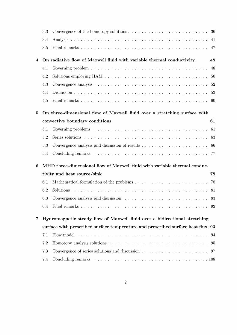
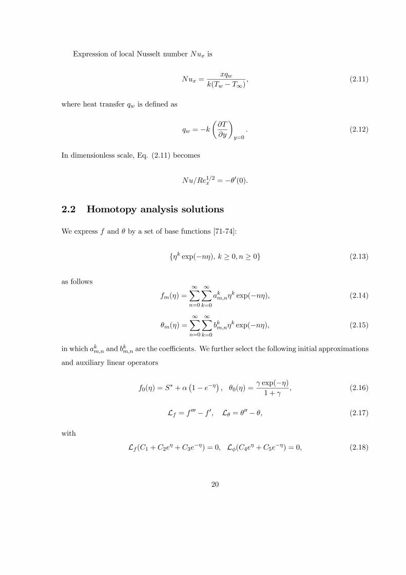
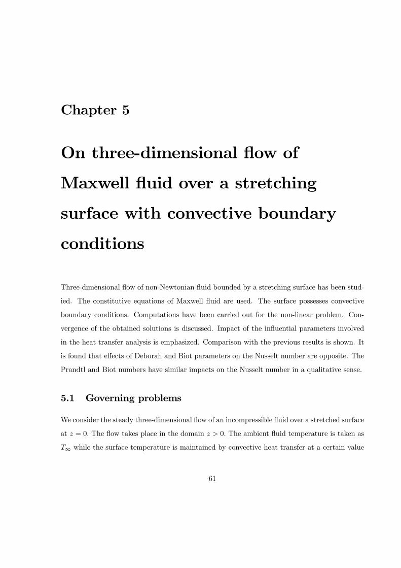
admissible values of ~ and ~ the ~−curves have been potrayed for 20-order of approxima-tions. Fig. 2.1 shows that the range of admissible values of ~ and ~ are −24 ≤ ~ ≤ −02and −21 ≤ ~ ≤ −04 The series converges in the whole region of when ~ = ~ = −14
-2.5 -2 -1.5 -1 -0.5 0Ñf, Ñq
-0.6
-0.5
-0.4
-0.3
-0.2
f''0
,q'0
Pr =1.0, a =0.3, S* =0.5, g = 1.0, b = 0.2
q'0f''0
Fig. 2.1: ~−curves for the functions () and ()
Table: 2.1. Convergence of homotopy solution for different order of approximations when
= 02 = 03 = 10 ∗ = 05 = 10 and ~ = ~ = −14
Order of approximation − 00(0) −0(0)1 0.2829900 0.4300000
5 0.2814982 0.4064811
10 0.2814950 0.4047923
20 0.2814950 0.4046587
30 0.2814950 0.4046572
35 0.2814950 0.4046572
40 0.2814950 0.4046572
23

2.4 Graphical results and discussion
In this section our main interest is to discuss the influence of emerging parameters such as
stretching parameter Deborah number suction parameter ∗ Prandtl number Pr and
Biot number on the velocity and temperature fields. The analysis of such variations is made
through the Figs. 22 − 29 Figs. 22 − 24 are displayed to see the effects of and ∗ on
the velocity field 0 As increases in Fig. 22 the flow velocity enhances. Fig. 2.3 shows the
effects of on 0 It is obvious from this Fig. that 0 is a decreasing function of This is due
to the fact that Deborah number depends upon the relaxation time and an increase in Deborah
number leads to an increase in the relaxation time. Such increase in relaxation time decrease
the fluid velocity and momentum boundary layer thickness. The same behavior is observed as
the suction parameter ∗ increases in Fig. 2.4. It is seen that the boundary layer thickness
decreases with increasing values of ∗ 0 In fact suction is an agent which resists the fluid
flow due to which the velocity is reduced. Figs. 2.5-2.9 depict the influences of ∗
and on the temperature profile Fig. 2.5 describes the effects of on Here decreases
when Pr increases. Physically, Prandtl number is the ratio of momentum to thermal diffusivity.
Higher values of Prandtl number implies the higher momentum diffusivity and lower thermal
diffusivity. This lower thermal diffusivity corresponds to a lower temperature and thinner
thermal boundary layer thickness. The proper value of Prandtl number is quite essential to
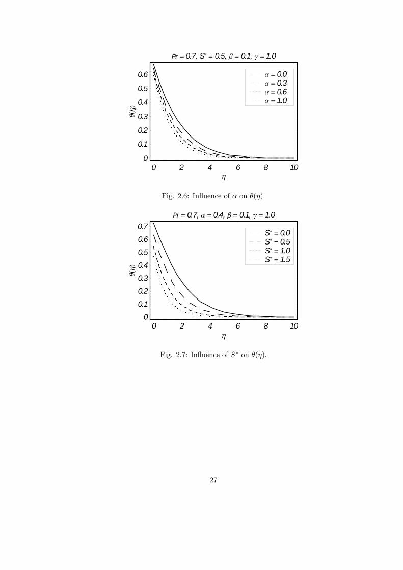
control the heat transfer in industrial processes. Fig. 2.6 indicates that is a decreasing
function of In Fig. 2.7 the variation of temperature is plotted for the different values of ∗
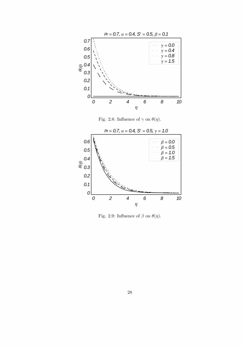
The temperature profile decreases by increasing ∗ Fig. 2.8 shows the influence of Biot number
on Temperature field enhances by increasing Here heat transfer coefficient is larger for
higher Biot number which gives rsie to the temperature and thermal boundary layer thickness.
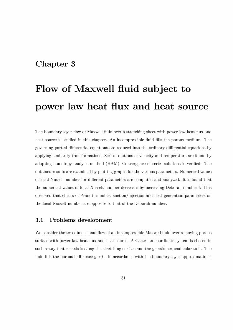
Fig. 2.9 is plotted to see the effects of on temperature profile It has been seen from
this Fig. that temperature is an increasing function of Table 2.1 is computed to analyze the
convergence values of − 00(0) and −0(0) at different order of HAM approximations. This Table
depicts that less deformations are required for the velocity in comparison to the temperature
for a convergent solution. Table 2.2 includes the values of local Nusselt number for different
values and when ∗ = 05 and = 02 The values of local Nusselt number are larger
24

for higher values of and Such values are smaller for the higher values of
0 1 2 3 4 5 6h
0
0.2
0.4
0.6
0.8
1
f'h
S* = 0.5, b = 0.1
a = 1.0a = 0.6a = 0.3a = 0.0
Fig. 2.2: Influence of on 0()
0 2 4 6 8h
0
0.1
0.2
0.3
0.4
f'h
a = 0.4, S* = 0.5
b = 1.5b = 1.0b = 0.5b = 0.0
Fig. 2.3: Influence of on 0()
25

0 2 4 6 8 10h
0
0.1
0.2
0.3
0.4
f'h
a = 0.4, b = 0.1
S* = 1.5S* = 1.0S* = 0.5S* = 0.0
Fig. 2.4: Influence of ∗ on 0()
0 2 4 6 8 10h
0
0.1
0.2
0.3
0.4
0.5
0.6
0.7
qh
a = 0.4, S* = 0.5, b = 0.1, g = 1.0
Pr = 1.5Pr = 1.0Pr = 0.5Pr = 0.1
Fig. 2.5: Influence of on ()
26
0 2 4 6 8 10h
0
0.1
0.2
0.3
0.4
0.5
0.6
qh
Pr = 0.7, S* = 0.5, b = 0.1, g = 1.0
a = 1.0a = 0.6a = 0.3a = 0.0
Fig. 2.6: Influence of on ()
0 2 4 6 8 10h
0
0.1
0.2
0.3
0.4
0.5
0.6
0.7
qh
Pr = 0.7, a = 0.4, b = 0.1, g = 1.0
S* = 1.5S* = 1.0S* = 0.5S* = 0.0
Fig. 2.7: Influence of ∗ on ()
27
0 2 4 6 8 10h
0
0.1
0.2
0.3
0.4
0.5
0.6
0.7
qh
Pr = 0.7, a = 0.4, S* = 0.5, b = 0.1
g = 1.5g = 0.8g = 0.4g = 0.0
Fig. 2.8: Influence of on ()
0 2 4 6 8 10h
0
0.1
0.2
0.3
0.4
0.5
0.6
qh
Pr = 0.7, a = 0.4, S* = 0.5, g = 1.0
b = 1.5b = 1.0b = 0.5b = 0.0
Fig. 2.9: Influence of on ()
28

Table 2.2: Values of local Nusselt number −12 for the parameters and when
∗ = 05 and = 02
−12
0.5 1.0 0.1 0.23336
1.0 0.36588
1.5 0.45796
2.0 0.52558
1.0 0. 0.3189
0.5 0.26799
1.0 0.36591
2.0 0.2039
0.1 0.36588
0.3 0.40466
0.8 0.45825
1.0 0.47254
2.5 Concluding remarks
Here we considered the effects of heat transfer in the flow of a Maxwell fluid over a stretching wall
with convective boundary conditions. The graphical results reflecting the effects of interesting
parameters are analyzed. The main results are as follows:
• By increasing the velocity field 0 increases.
• The velocity profile 0 decreases by increasing Deborah number and suction parameter∗
• Increase in Prandtl number decreases the temperature profile
• The effects of Biot number and Deborah number on are similar in a qualitative
sense.
• Increasing values of Biot number lead to higher temperature and thermal boundary layer
29

thickness.
30
Chapter 3
Flow of Maxwell fluid subject to
power law heat flux and heat source
The boundary layer flow of Maxwell fluid over a stretching sheet with power law heat flux and
heat source is studied in this chapter. An incompressible fluid fills the porous medium. The
governing partial differential equations are reduced into the ordinary differential equations by
applying similarity transformations. Series solutions of velocity and temperature are found by
adopting homotopy analysis method (HAM). Convergence of series solutions is verified. The
obtained results are examined by plotting graphs for the various parameters. Numerical values
of local Nusselt number for different parameters are computed and analyzed. It is found that
the numerical values of local Nusselt number decreases by increasing Deborah number It is
observed that effects of Prandtl number, suction/injection and heat generation parameters on
the local Nusselt number are opposite to that of the Deborah number.
3.1 Problems development
We consider the two-dimensional flow of an incompressible Maxwell fluid over a moving porous
surface with power law heat flux and heat source. A Cartesian coordinate system is chosen in
such a way that −axis is along the stretching surface and the −axis perpendicular to it. Thefluid fills the porous half space 0. In accordance with the boundary layer approximations,
31

the governing equations for flow and temperature are
+
= 0 (3.1)
+
=
2
2− 1
∙2
2
2+ 2
2
2+ 2
2
¸−
(3.2)
+
=
2
2−
( − ∞) (3.3)
where and are the velocity components in the − and −directions, 1 is the relaxationtime, = () is the kinematic viscosity, is the permeability of porous medium, is the
fluid temperature, is the density of fluid, is the thermal conductivity of fluid, is the
specific heat at constant pressure and is the heat source coefficient.
The boundary conditions are taken in the forms:
= = −0
= 2 at = 0 (3.4)
= 0 = ∞ as →∞ (3.5)
where is the temperature coefficient and ∞ is the fluid temperature far away from the sheet.
We introduce the transformations
= 0() = −√() = ∞ +
r
2() =
r
(3.6)
Here is a constant and prime denotes differentiation with respect to .
Equations (32)− (35) yield
000 + 00 − 02 + (2 0 00 − 2 000)− 0 = 0 (3.7)
00 + 0 − 2 0 − ∗ = 0 (3.8)
= ∗ 0 = 1 0 = 1 at = 0 (3.9)
0 = 0 = 0 as →∞ (3.10)
32
where Eq. (31) is satisfied automatically and = 1 is the Deborah number =
is the
permeability parameter, ∗ = 0√is the suction parameter, =
is the Prandtl number
and ∗ = is a heat generation parameter.
Expression of local Nusselt number is
=
( − ∞) (3.11)
where heat transfer can be defined as
= −µ
¶=0
(3.12)
In dimensionless form, Eq. (311) becomes
12 = − 1
(0) (3.13)
3.2 Homotopy analysis solutions
Considering a set of base functions
{ exp(−) ≥ 0 ≥ 0} (3.14)
we write
() =
∞X=0
∞X=0
exp(−) (3.15)
() =
∞X=0
∞X=0
exp(−) (3.16)
in which and are the coefficients. The initial approximations and auxiliary linear
operators are taken in the forms:
0() = ∗ + 1− exp(−) 0() = − exp(−) (3.17)
L = 000 − 0 L = 00 + 0 (3.18)
33
with
L (1 + 2 + 3
−) = 0 L(4 + 5−) = 0 (3.19)
where ( = 1− 5) represent the arbitrary constants.The zeroth order deformation problems are [75-78]:
(1− )Lh(; )− 0()
i= ~N
h(; )
i (3.20)
(1− )Lh(; )− 0()
i= ~N
h(; ) ( )
i (3.21)
(0; ) = ∗ 0(0; ) = 1 0(∞; ) = 0 0(0 ) = 1 (∞ ) = 0 (3.22)
N [( )] =3( )
3− ( )
2( )
2−Ã( )
!2
+
"2( )
( )
2( )
2− (( ))2
3( )
3
#−
( )
(3.23)
N[( ) ( )] =2( )
2+ ( )
( )
− 2( )
( )− ∗( ) (3.24)
in which is an embedding parameter, ~ and ~ the non zero auxiliary parameters and N
and N the nonlinear operators.
For = 0 and = 1 we have
(; 0) = 0() ( 0) = 0() and (; 1) = () ( 1) = () (3.25)
and when increases from 0 to 1 then ( ) and ( ) approach from 0() 0() to ()
and () By Taylor’s series one has
( ) = 0() +∞P
=1
() (3.26)
( ) = 0() +∞P
=1
() (3.27)
() =1
!
(; )
¯=0
() =1
!
(; )
¯=0
(3.28)
34
where the convergence of above series strongly depends upon ~ and ~ Considering that ~
and ~ are selected properly so that Eqs. (326) and (327) converge at = 1 and thus we have
() = 0() +∞P
=1
() (3.29)
() = 0() +∞P
=1
() (3.30)
The problems at th-order are
L [()− −1()] = ~R () (3.31)
L[()− −1()] = ~R () (3.32)
(0) = 0(0) = 0(∞) = 0 0(0)− (0) = (∞) = 0 (3.33)
R () = 000−1() +
−1P=0
h−1− 00 − 0−1−
000
i+
−1X=0
−1−X=0
{2 0− 00 − − 000 − 0−1() (3.34)
R () = 00−1 +
−1P=0
0−1− − 2−1P=0
−1− 0 − ∗ (3.35)
=
⎡⎣ 0 ≤ 11 1
(3.36)
The general solutions can be expressed in the forms
() = ∗() + 1 + 2 + 3
− (3.37)
() = ∗() + 4 + 5− (3.38)
in which ∗ and ∗ indicate the special solutions.
35
3.3 Convergence of the homotopy solutions
In this section, we discuss the convergence of the series given in Eqs. (329) and (330) For
this we first show that if the series (315) and (316) converge then these will converge to the
solution of the problem given by Eqs. (37)− (310) Let us suppose that ~ and ~ are selectedsuch that the series (315) and (316) converge. Therefore we have
lim→∞
() = 0, lim→∞
() = 0 (3.39)
From Eqs. (331), (332) and (336) one has
lim→∞
"~
X=1
R ()
#= lim
→∞
X=1
L [ − −1]
= lim→∞
L"
X=1
−X=1
−1
#= lim
→∞L = L lim
→∞ = 0 ∈ [0∞] (3.40)
lim→∞
"~
X=1
R ()
#= lim
→∞
X=1
L [ − −1]
= lim→∞
L"
X=1
−X=1
−1
#= lim
→∞L = L lim
→∞ = 0 ∈ [0∞] (3.41)
Equations (340) and (341) imply that the infinite sequence 1, 2, 3, , and 1, 2, 3, Ãwhere =
X=1
R () , =
X=1
R ()
!converge to zero. Now
X=1
R () =
X=1
⎧⎪⎪⎨⎪⎪⎩ 000−1 ()− 0−1 () +−1X=0
⎡⎢⎢⎣ −1− 00 − 0−1− 0
+−1−X=0
©2 0−
00 − − 000
ª⎤⎥⎥⎦⎫⎪⎪⎬⎪⎪⎭
(3.42)
36
lim→∞
"X=1
R ()
#=
∞X=1
⎧⎪⎪⎪⎪⎪⎨⎪⎪⎪⎪⎪⎩ 000−1 ()− 0−1 ()
+
−1X=0
⎡⎢⎢⎣ −1− 00 − 0−1− 0
+−1−X=0
©2 0−
00 − − 000
ª⎤⎥⎥⎦
⎫⎪⎪⎪⎪⎪⎬⎪⎪⎪⎪⎪⎭
=
⎧⎪⎪⎪⎪⎪⎪⎪⎨⎪⎪⎪⎪⎪⎪⎪⎩
3
3
à ∞X=1
−1 ()
!−
à ∞X=1
−1 ()
!
+
∞X=1
−1X=0
⎡⎢⎢⎣ −1− 00 − 0−1− 0
+−1−X=0
©2 0−
00 − − 000
ª⎤⎥⎥⎦
⎫⎪⎪⎪⎪⎪⎪⎪⎬⎪⎪⎪⎪⎪⎪⎪⎭
=
⎧⎪⎪⎪⎪⎪⎪⎪⎨⎪⎪⎪⎪⎪⎪⎪⎩
3
3
à ∞X=0
()
!−
à ∞X=0
()
!
+
∞X=0
∞X=+1
⎡⎢⎢⎣ −1− 00 − 0−1− 0
+−1−∞X=
©2 0−
00 − − 000
ª⎤⎥⎥⎦
⎫⎪⎪⎪⎪⎪⎪⎪⎬⎪⎪⎪⎪⎪⎪⎪⎭
=
⎧⎪⎪⎪⎪⎪⎪⎪⎪⎪⎪⎪⎪⎪⎪⎪⎪⎪⎪⎪⎪⎨⎪⎪⎪⎪⎪⎪⎪⎪⎪⎪⎪⎪⎪⎪⎪⎪⎪⎪⎪⎪⎩
3
3
à ∞X=0
()
!−
à ∞X=0
()
!+Ã ∞X
=0
()
!Ã2
2
" ∞X=0
()
#!−Ã
" ∞X=0
()
#!2−
à ∞X=0
()
!23
3
" ∞X=0
()
#+
à ∞X=0
()
!Ã
" ∞X=0
()
#!2
2
" ∞X=0
()
#
⎫⎪⎪⎪⎪⎪⎪⎪⎪⎪⎪⎪⎪⎪⎪⎪⎪⎪⎪⎪⎪⎬⎪⎪⎪⎪⎪⎪⎪⎪⎪⎪⎪⎪⎪⎪⎪⎪⎪⎪⎪⎪⎭
(3.43)
and
X=1
R () =
X=1
(00−1 ()− ∗−1 () + Pr
−1X=0
£0−1− − 2−1− 0
¤) (3.44)
37
lim→∞
"X=1
R ()
#=
∞X=1
⎧⎪⎪⎨⎪⎪⎩00−1 ()− ∗−1 ()
+
−1X=0
£0−1− − 2−1− 0
¤⎫⎪⎪⎬⎪⎪⎭
=
⎧⎪⎪⎪⎪⎨⎪⎪⎪⎪⎩2
2
à ∞X=1
−1 ()
!− ∗
à ∞X=1
−1 ()
!
+
∞X=1
−1X=0
£0−1− − 2−1− 0
¤⎫⎪⎪⎪⎪⎬⎪⎪⎪⎪⎭
=
⎧⎪⎪⎪⎪⎨⎪⎪⎪⎪⎩2
2
à ∞X=1
−1 ()
!− ∗
à ∞X=1
−1 ()
!+
∞X=0
∞X=+1
£0−1− − 2−1− 0
¤⎫⎪⎪⎪⎪⎬⎪⎪⎪⎪⎭
=
⎧⎪⎪⎪⎪⎪⎪⎪⎪⎪⎨⎪⎪⎪⎪⎪⎪⎪⎪⎪⎩
2
2
à ∞X=1
−1 ()
!− ∗
à ∞X=1
−1 ()
!
+
à ∞X=0
()
!Ã
" ∞X=0
()
#!
−2Ã
" ∞X=0
()
#!Ã ∞X=0
()
!
⎫⎪⎪⎪⎪⎪⎪⎪⎪⎪⎬⎪⎪⎪⎪⎪⎪⎪⎪⎪⎭(3.45)
and therefore the above equations after using Eq. (339) become
⎧⎪⎪⎪⎪⎪⎪⎪⎪⎪⎨⎪⎪⎪⎪⎪⎪⎪⎪⎪⎩
3
3
à ∞X=0
()
!−
à ∞X=0
()
!+
à ∞X=0
()
!Ã2
2
" ∞X=0
()
#!
−Ã
" ∞X=0
()
#!2−
à ∞X=0
()
!23
3
" ∞X=0
()
#
+
à ∞X=0
()
!Ã
" ∞X=0
()
#!2
2
" ∞X=0
()
#
⎫⎪⎪⎪⎪⎪⎪⎪⎪⎪⎬⎪⎪⎪⎪⎪⎪⎪⎪⎪⎭= 0 (3.46)
⎧⎪⎪⎪⎪⎨⎪⎪⎪⎪⎩2
2
à ∞X=1
−1 ()
!− ∗
à ∞X=1
−1 ()
!+
à ∞X=0
()
!Ã
" ∞X=0
()
#!
−2Ã
" ∞X=0
()
#!Ã ∞X=0
()
!⎫⎪⎪⎪⎪⎬⎪⎪⎪⎪⎭ = 0 (3.47)
38
From Eq. (333) we now write
∞X=0
(0) = 0
∞X=0
0 (0) = 0∞X=0
0 (∞) = 0∞X=0
£0 (0)− (0)
¤= 0
∞X=0
(∞) = 0
(3.48)
Equations (346)−(348) show that if the series (315) and (316) converge, it must be a solutionof the presented problem. Thus the only requirement to choose the appropriate initial guesses
0 () 0 (), auxiliary linear operators L , L and the auxiliary parameters ~ and ~ to ensurethat the infinite series (315) and (316) are convergent.
The convergence region and rate of convergence of the series (315) and (316) strongly
depends upon the values of ~ and ~ Here the question arises that how one can select the valid
region for the values of ~ and ~ so that the solution series (315) and (316) are convergent. If
we closely look into equations (37)− (310) then for the dependent variable () there is onemissing condition 00 (0) and for the variable () the missing condition is 00(0). Therefore we
look for the convergence of the related series 00 (0) and 00 (0). If we plot these series against
the parameters ~ and ~ the curves obtained in this way are called ~-curves. We first draw
the ~-curves for the series 00 (0) and 00 (0). The portion of the ~-curves which is parallel to
the ~-axis will give the region for the admissible values of ~ and ~ and it actually gives the
values of the missing conditions for both the dependent variables. Once we get the values of
the missing conditions we can then find the solution of the problem.
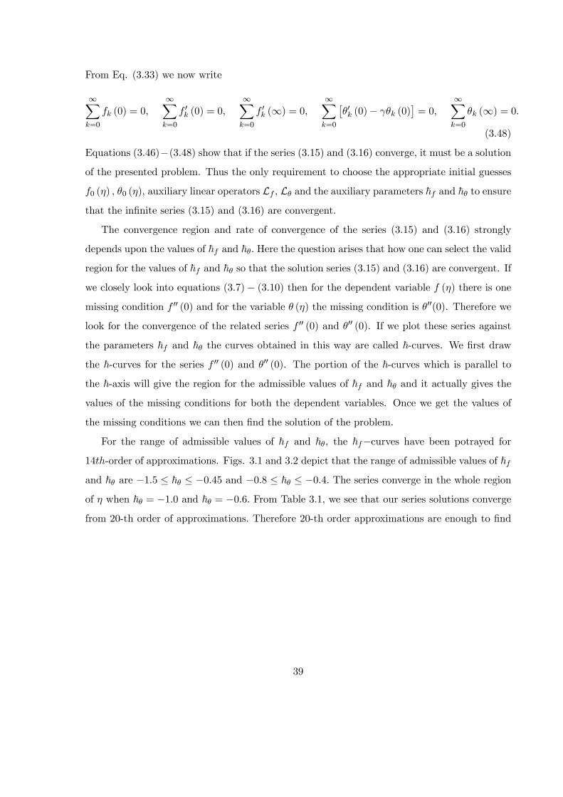
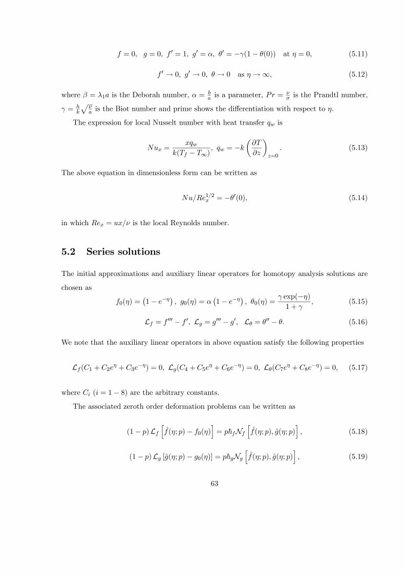
For the range of admissible values of ~ and }, the ~−curves have been potrayed for14-order of approximations. Figs. 31 and 32 depict that the range of admissible values of }
and } are −15 ≤ ~ ≤ −045 and −08 ≤ ~ ≤ −04 The series converge in the whole regionof when ~ = −10 and ~ = −06 From Table 31 we see that our series solutions converge
from 20-th order of approximations Therefore 20-th order approximations are enough to find
39
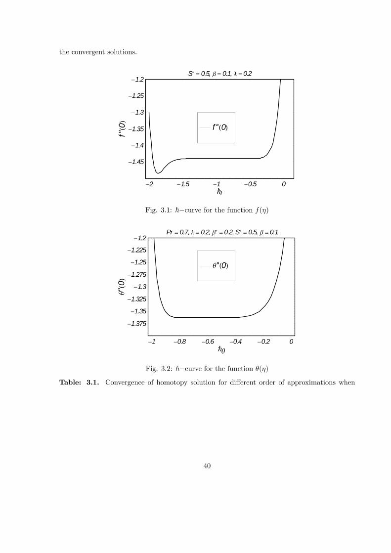
the convergent solutions.
-2 -1.5 -1 -0.5 0Ñf
-1.45
-1.4
-1.35
-1.3
-1.25
-1.2
f''0
S* = 0.5, b= 0.1, l =0.2
f ''0
Fig. 3.1: ~−curve for the function ()
-1 -0.8 -0.6 -0.4 -0.2 0Ñq
-1.375
-1.35
-1.325
-1.3
-1.275
-1.25
-1.225
-1.2
q''0
Pr = 0.7, l = 0.2, b* =0.2, S* = 0.5, b =0.1
q''0
Fig. 3.2: ~−curve for the function ()
Table: 3.1. Convergence of homotopy solution for different order of approximations when
40
= 02 = 03 = 10, ∗ = 05 = 10 and } = −10 and ~ = −06
Order of approximation − 00(0) −00(0)1 1.38750 1.27000
5 1.44009 1.36626
10 1.44007 1.36263
15 1.44007 1.36280
20 1.44007 1.36279
25 1.44007 1.36279
30 1.44007 1.36279
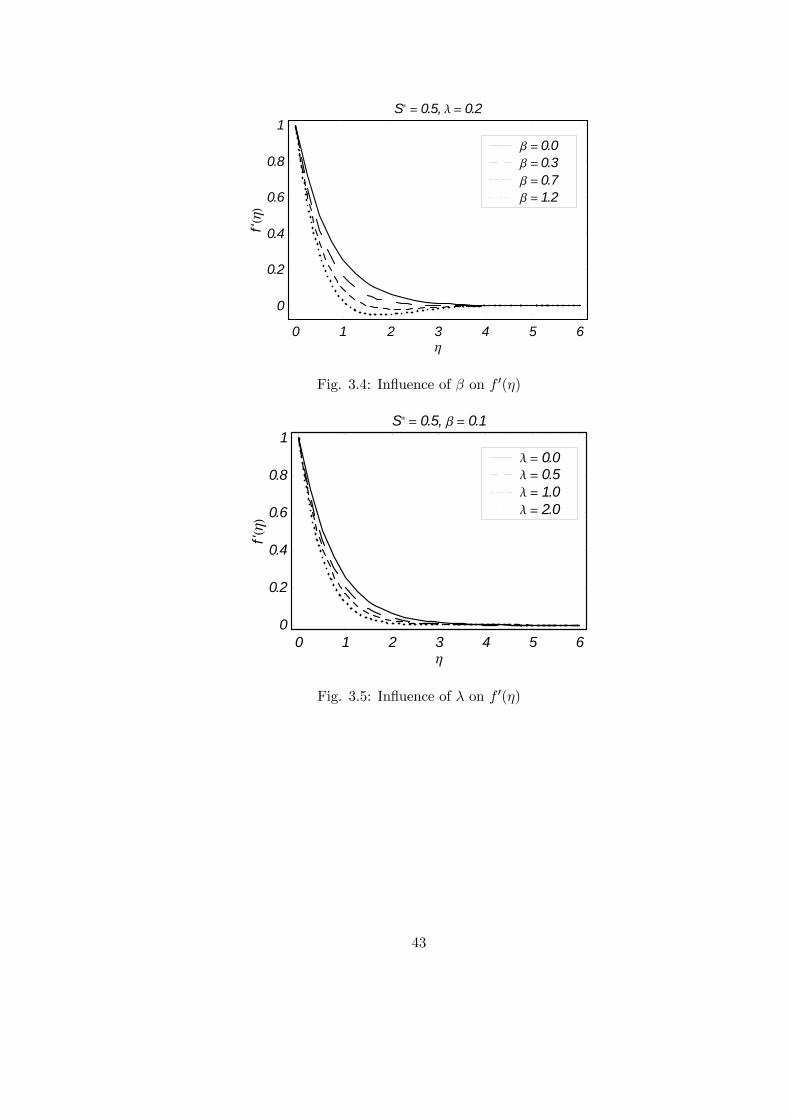
3.4 Analysis
The objective of this section is to predict the influences of different parameters ∗
and ∗ on velocity 0() and temperature () fields For this aim we plotted Figs. 33− 310for various interesting parameters on velocity and temperature fields. Figs. 33− 35 representthe variations of suction parameter ∗ Deborah number and permeability parameter on
velocity profile 0() Fig. 33 depicts the effects of ∗ on 0() From Fig. 33, we noted
that the velocity profile 0() decreases by increasing ∗ The Deborah number decreases the
velocity field 0() (see Fig. 34) Hence we can say that the velocity field 0() is a decreasing
function of Deborah number is directly proportional to relaxation time. An increasing values
of Deborah number correspond to higher relaxation time. Such higher relaxation time is caused
a reduction in the fluid velocity. Fig. 35 represents the effect of on 0() The velocity
profile decreases when is increased The permeability of porous medium is decreased with
an increase in that leads to the lower velocity and thinner boundary layer thickness. Figs.
36− 310 are drawn to see the behaviors of ∗ and ∗ on the temperature field ()
Fig. 36 describes the effects of suction parameter ∗ on () We note that ∗ leads to a
decrease in the temperature profile. Fig. 37 plots the effects of on () The temperature
field () increases by increasing The effects of permeability parameter on () have been
illustrated in Fig. 38 We see that the temperature field () increases by increasing Figs.
39 and 310 depict the effects of and on () From Figs. 39 and 310 we observed that
41

the increase in and decreases the temperature field. We conclude that both and ∗
have same qualitative effects on the temperature profile () Physically ∗ 0 implies that
∞ the supply of heat to the flow region is from the wall. Fig. 3.10 depicts that if more
fluid is injected then the temperature decreases due to a great loss of heat from hot injection.
Here the temperature is negative for all the cases. Table 3.2 presents the numerical values of
local Nusselt number for different values of embedded parameters. The local Nusselt number
increases by increasing suction parameter and Prandtl number but it decreases when we
increase Deborah number and heat generation parameter ∗
0 1 2 3 4 5 6h
0
0.2
0.4
0.6
0.8
1
f'h
b = 0.1, l = 0.2
S* = 2.0S* = 1.0S* = 0.5S* = 0.0
Fig. 3.3: Influence of ∗ on 0()
42
0 1 2 3 4 5 6h
0
0.2
0.4
0.6
0.8
1
f'h
S* = 0.5, l = 0.2
b = 1.2b = 0.7b = 0.3b = 0.0
Fig. 3.4: Influence of on 0()
0 1 2 3 4 5 6h
0
0.2
0.4
0.6
0.8
1
f'h
S* = 0.5, b = 0.1
l = 2.0l = 1.0l = 0.5l = 0.0
Fig. 3.5: Influence of on 0()
43

0 2 4 6 8 10h
-0.8
-0.6
-0.4
-0.2
0
qh
b = 0.1, l = 0.2, Pr = 0.7, b* = 0.2
S* = 1.5S* = 1.0S* = 0.4S* = 0.0
Fig. 3.6: Influence of ∗ on ()
0 2 4 6 8 10h
-0.8
-0.6
-0.4
-0.2
0
qh
S* = 0.5, l = 0.2, Pr = 0.7, b* = 0.2
b = 1.5b = 0.7b = 0.3b = 0.0
Fig. 3.7: Influence of on ()
44
0 2 4 6 8 10h
-0.8
-0.6
-0.4
-0.2
0
qh
b = 0.1, S* = 0.5, Pr = 0.7, b* = 0.2
l = 1.5l = 0.8l = 0.4l = 0.0
Fig. 3.8: Influence of on ()
0 2 4 6 8 10h
-1.5
-1.25
-1
-0.75
-0.5
-0.25
0
qh
S* = 0.5, b = 0.1, l = 0.2, b* = 0.2
Pr = 1.2Pr = 0.7Pr = 0.3Pr = 0.1
Fig. 3.9: Influence of on ()
45
0 2 4 6 8 10h
-0.8
-0.6
-0.4
-0.2
0
qh
S* = 0.5, b = 0.1, l = 0.2, Pr = 0.7
b* = 1.0b* = 0.6b* = 0.3b* = 0.0
Fig. 3.10: Influence of ∗ on ()
Table 3.2: Values of local Nusselt number 12 for the parameters ∗ and ∗
when = 01
∗ ∗ −12
0.0 0.5 0.5 0.2 1.09743
0.2 1.05938
0.5 1.00375
0.3 0.83400
0.5 1.07838
1.0 1.63452
0.0 0.98824
0.5 1.07839
1.0 1.17777
0.0 0.91655
0.4 1.19972
0.8 1.39493
46

3.5 Final remarks
We studied the steady flow of Maxwell fluid over a stretching surface in presence of power law
heat flux and heat source. The series solutions have been developed to analyze the salient
features of this work. We noticed that the suction parameter and Deborah number have
similar effects on velocity profile 0() in a qualitative sense. Velocity field 0() decreases by
increasing permeability parameter It is observed that the temperature profile () increases
in view of an increase in and Also we have seen that the heat generation parameter ∗
leads to a decrease in the temperature ()
47
Chapter 4
On radiative flow of Maxwell fluid
with variable thermal conductivity
This chapter extends the analysis of previous chapter for variable thermal conductivity. The
governing nonlinear partial differential equations are reduced into the ordinary differential equa-
tions by appropriate transformations. The solution of temperature is presented. The variations
of various embedded parameters on the temperature are displayed and discussed. The values
of local Nusselt number are compared with the existing numerical solution in a limiting sense.
4.1 Governing problem
The energy equation in presence of thermal radiation is given by
µ
+
¶=
µ
¶−
(4.1)
In view of Rosseland approximation [35], we have = (−43∗) 4 Expanding 4 about∞ by Taylor series and neglecting higher-order terms we obtain, 4 = 4 3∞ −3 4∞ Equation(4.1) thus can be written as
µ
+
¶=
µ
¶− 16
3∞3∗
2
2 (4.2)
48
The boundary conditions are presented by
= () = ∞ +1 at = 0 (4.3)
→ ∞ as →∞ (4.4)
where is the variable thermal conductivity, the density of fluid, the specific heat at
constant pressure, the Stefan-Boltzmann constant and ∗ the mean absorption coefficient.
We consider the transformation
() = − ∞ − ∞
(4.5)
with () = ∞ +1() at = 0 and variable thermal conductivity = ∞[1 + ] (∞
is the fluid free stream conductivity) and is defined by
=( − ∞)
∞ (4.6)
in which is the fluid thermal conductivity at the wall.
The above transformations satisfy the incompressibility condition and now Eq. (42) yields
(1 + )00 + 02 +4
300 = [1
0 − 0] (4.7)
(0) = 1, (∞) = 0 (4.8)
where = 1 is the Deborah number = () is the permeability parameter, =∞ is
the Prandtl number and =4 3∞∞∗ is the radiation parameter.
The local Nusselt number with heat transfer is given by
=
( − ∞) = −
µ
¶=0
(4.9)
In dimensionless scale, Eq. (49) becomes
12 = −0(0) (4.10)
49
4.2 Solutions employing HAM
We express in the set of base function
{ exp(−) ≥ 0 ≥ 0} (4.11)
as follows
() =
∞X=0
∞X=0
exp(−) (4.12)
in which is the coefficient.
The initial approximations and auxiliary linear operators are given below
0() = (−) (4.13)
L = 00 − (4.14)
with
L(1 + 2−) = 0 (4.15)
where ( = 1 2) denotes the arbitrary constants. The following problems corresponding to
the zeroth order deformations are constructed as follows:
(1− )Lh(; )− 0()
i= ~N
h(; ) ( )
i (4.16)
(0 ) = 1 0(∞ ) = 0 (4.17)
N[( ) ( )] =
µ1 +
4
3
¶2( )
2+ ( )
2( )
2+
Ã( )
!2
−1( )( )
+ ( )( )
(4.18)
where is an embedding parameter, ~ is the non zero auxiliary parameters andN the nonlinear
50
operator. Note that for = 0 and = 1 we have
( 0) = 0() and ( 1) = () (4.19)
and when increases from 0 to 1 then ( ) varies from 0() to () By using Taylor’s series
we obtain
( ) = 0() +∞P
=1
() (4.20)
() =1
!
(; )
¯=0
(4.21)
where the convergence of above series strongly depends upon ~ Considering that ~ is selected
properly so that (420) converges at = 1 then
() = 0() +∞P
=1
() (4.22)
The problem at th-order are
L[()− −1()] = ~R () (4.23)
(0) = (∞) = 0 (4.24)
R () =
µ1 +
4
3
¶00−1 +
−1P=0
−1−00 + −1P=0
0−1−0
−1−1P=0
−1− 0 + −1P=0
−1− 0 (4.25)
=
⎡⎣ 0 ≤ 11 1
(4.26)
The general solutions are
() = ∗() +4 + 5
− (4.27)
in which ∗ denotes the special solutions.
51

4.3 Convergence analysis
We know that the expression (4.22) contains the nonzero auxiliary parameter ~ which can
adjust and control the convergence of the homotopy solutions. For admissible values of ~, the
~−curve has been potrayed for 22-order of approximations. Fig. 4.1 shows that the range foradmissible values of ~ are −12 ≤ ~ ≤ −03 The convergence of series solutions is obtainedin the whole region of when ~ = −07
-1.2 -1 -0.8 -0.6 -0.4 -0.2 0Ñq
-1.5
-1.25
-1
-0.75
-0.5
-0.25
0
q'0
Pr = 0.7, a1 =0.5, l= 2.0, N =0.3, b =0.1, e =0.2
q'0
Fig. 4.1: ~−curve for the function ()
Table: 4.1. Convergence of homotopy solutions for different order of approximations when
= 02 1 = 10 = 10, = 03 = 20 = 02 and } = −07
Order of approximation −0(0)1 0.76667
5 0.68252
10 0.66613
20 0.65959
30 0.65834
35 0.65819
40 0.65819
50 0.65819
52

4.4 Discussion
Here our interest is just to examine the role of interesting parameters on the velocity and
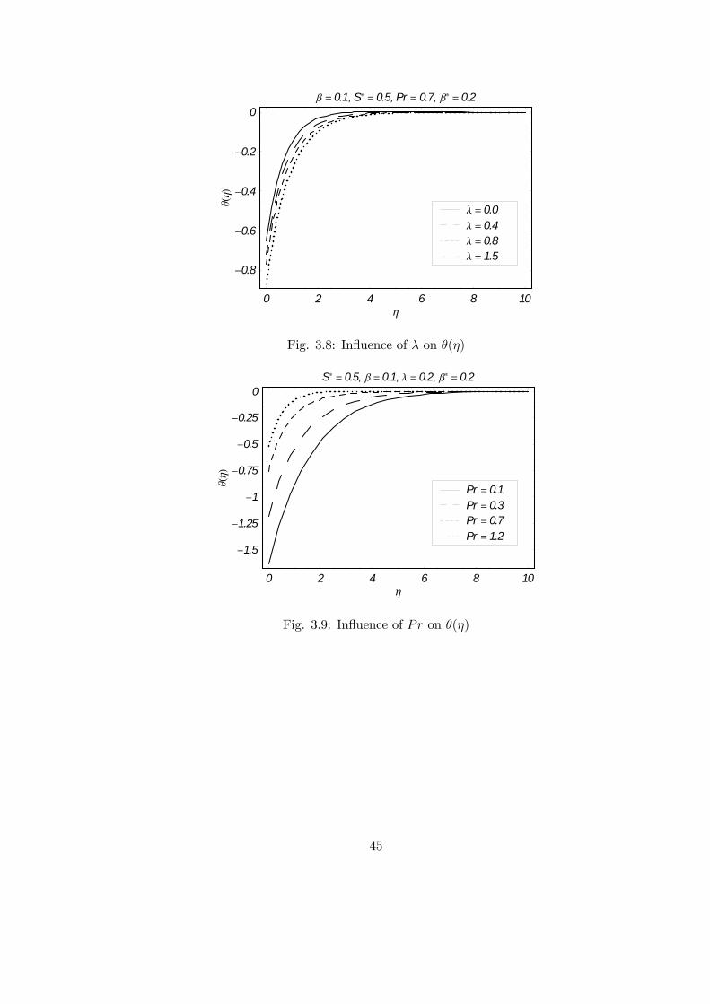
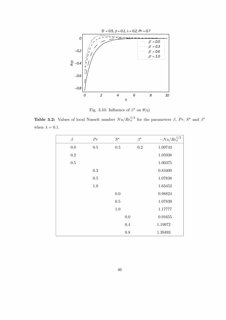
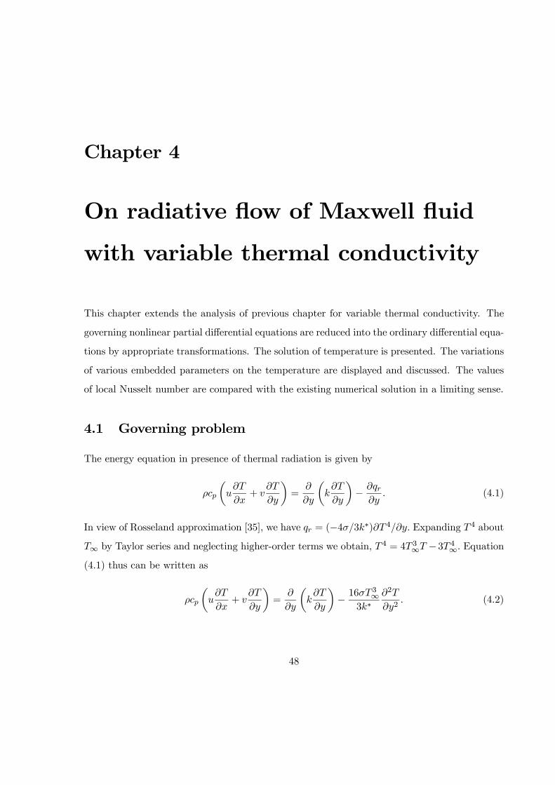
temperature. Hence the Figs. 4.2-4.7 have been plotted for Deborah number permeability
parameter Prandtl number positive constant 1 radiation parameter and small pa-
rameter on the temperature profile (). Fig. 4.2 represents the effects of on () Clearly
() increases when is increased. Fig. 4.3 illustrates that the temperature field () decreases
by increasing the permeability parameter The effects of on () are plotted in Fig. 4.4.
Here the temperature field () decreases by increasing In fact the definition of Prandtl
number involves the thermal diffusivity. When we increase the Prandtl number, a lower thermal
diffusivity occurs. Such lower thermal diffusivity caused a decrease in temperature. Fig. 4.5
shows the effects of 1 on () From Fig. 4.5 we observed that the temperature field ()
decreases when 1 increases. The temperature () and thermal boundary layer thickness are
increasing function of radiation parameter (Fig. 4.6). An increase in radiation augments the
heat transfer. The fluid is heated which increases the thermal boundary layer thickness. Fig.
4.7 represents the effects of on () The temperature () and associated thermal bound-
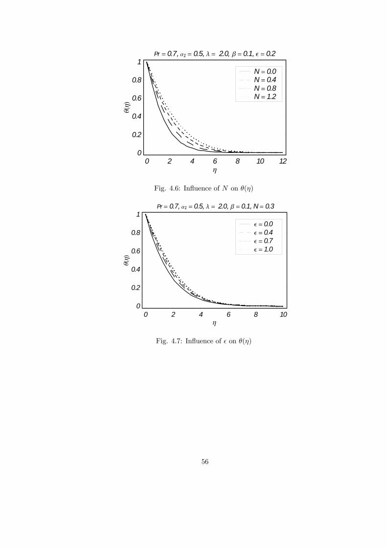
ary layer thickness increase when is increased. From Figs. 4.6 and 4.7 it is found that ()
increases when and are increased Hence and have similar role on the temperature
field () in a qualitative sense. Physically an increase in radiation parameter provides more
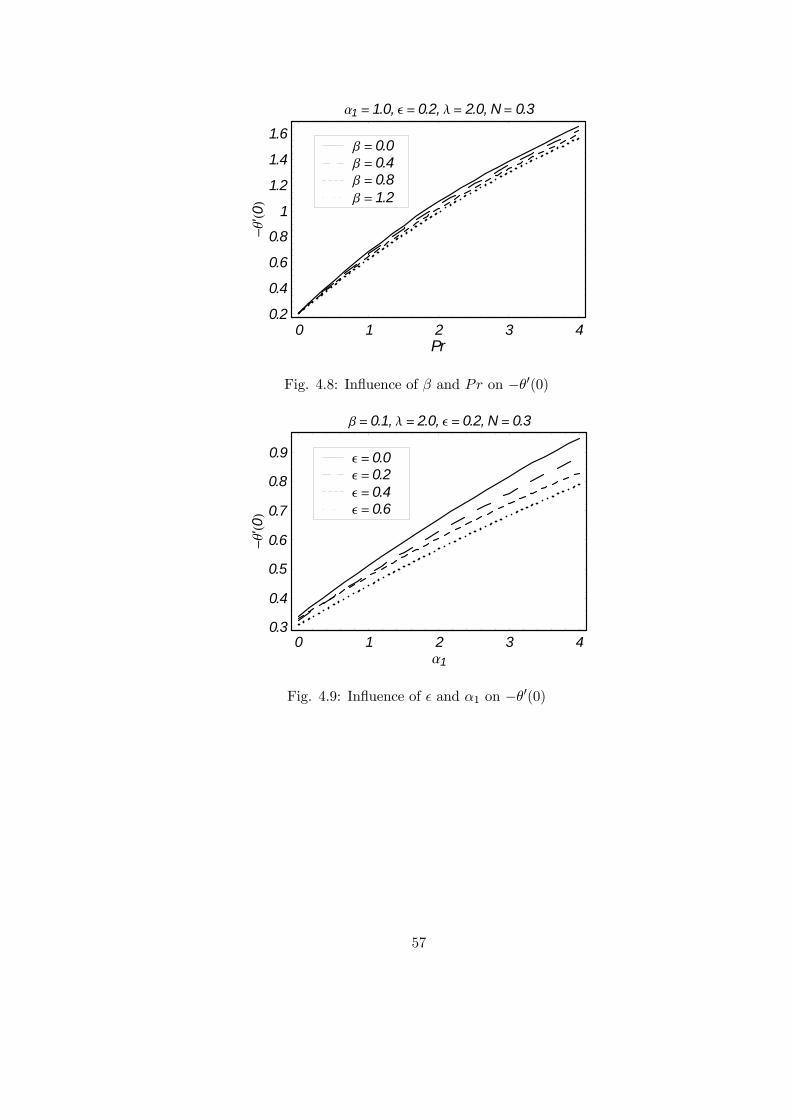
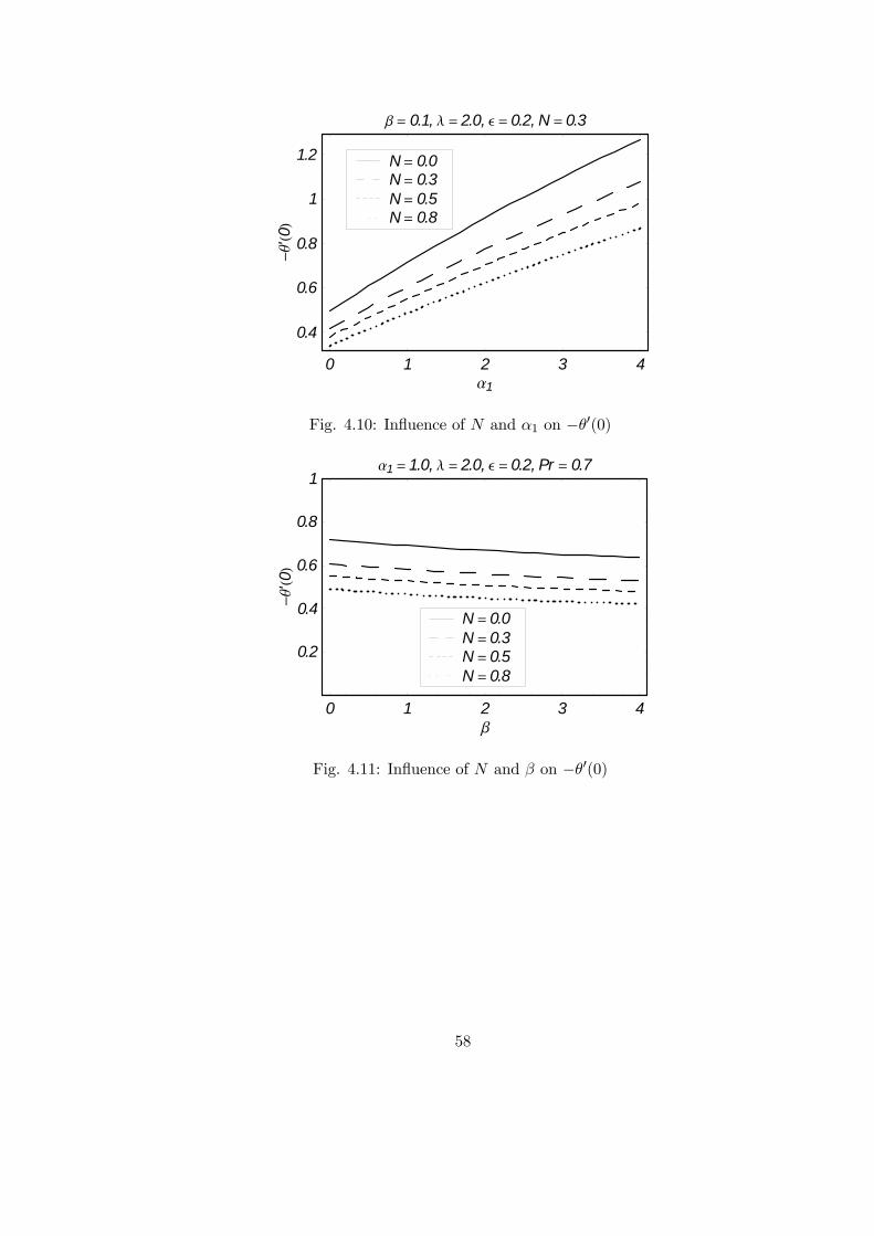
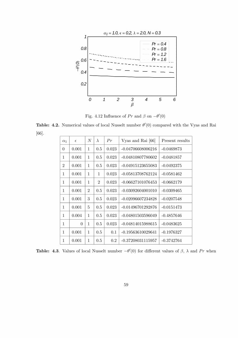
heat to fluid due to which higher temperature is observed. Figs. 4.8-4.12 are plotted to see
the influences of various emerging parameters on the local Nusselt number −0(0) Fig. 4.10illustrates the effects of and on the local Nusselt number. From this Fig. it is noted that
an increase in and leads to a decrease in local Nusselt number. Influences of and 1 on
the local Nusselt number are seen in Fig. 4.11. A decrease in local Nusselt number is observed
when and 1 are increased. Figs. 4.12 and 4.13 presented the effects of (1) and ()
on −0(0). These Figs. show that −0(0) is a decreasing function of (1) and () From
Fig. 4.14 we have seen that an increase in and corresponds to an enhancement in local
Nusselt number.
Table 4.1 shows the numerical values to ensure the convergence of series solutions. One can
see that our solutions for velocity converge from 10th order of approximations. However the
solutions for temperature converge from 35th order of deformations. Table 4.2 provides the
53
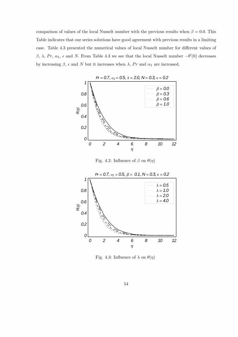
comparison of values of the local Nusselt number with the previous results when = 00 This
Table indicates that our series solutions have good agreement with previous results in a limiting
case. Table 4.3 presented the numerical values of local Nusselt number for different values of
1 and From Table 4.3 we see that the local Nusselt number −0(0) decreasesby increasing and but it increases when and 1 are increased.
0 2 4 6 8 10 12h
0
0.2
0.4
0.6
0.8
1qh
Pr = 0.7, a1= 0.5, l = 2.0, N= 0.3, e = 0.2
b = 1.0b = 0.6b = 0.3b = 0.0
Fig. 4.2: Influence of on ()
0 2 4 6 8 10 12h
0
0.2
0.4
0.6
0.8
1
qh
Pr = 0.7, a1 = 0.5, b = 0.1, N = 0.3, e = 0.2
l = 4.0l = 2.0l = 1.0l = 0.5
Fig. 4.3: Influence of on ()
54

0 2 4 6 8 10 12h
0
0.2
0.4
0.6
0.8
1
qh
a1= 0.5, l = 2.0, b = 0.1, N = 0.3, e = 0.2
Pr = 1.5Pr = 1.0Pr = 0.5Pr = 0.1
Fig. 4.4: Influence of on ()
0 2 4 6 8 10h
0
0.2
0.4
0.6
0.8
1
qh
Pr = 0.7, l = 2.0, b = 0.1, N = 0.3, e = 0.2
a1 = 3.0a1 = 2.0a1 = 1.0a1 = 0.0
Fig. 4.5: Influence of 1 on ()
55
0 2 4 6 8 10 12h
0
0.2
0.4
0.6
0.8
1
qh
Pr = 0.7, a1= 0.5, l = 2.0, b = 0.1, e = 0.2
N = 1.2N = 0.8N = 0.4N = 0.0
Fig. 4.6: Influence of on ()
0 2 4 6 8 10h
0
0.2
0.4
0.6
0.8
1
qh
Pr = 0.7, a1 = 0.5, l = 2.0, b = 0.1, N= 0.3
e = 1.0e = 0.7e = 0.4e = 0.0
Fig. 4.7: Influence of on ()
56
0 1 2 3 4Pr
0.2
0.4
0.6
0.8
1
1.2
1.4
1.6
-q'
0
a1 = 1.0, e = 0.2, l = 2.0, N= 0.3
b = 1.2b = 0.8b = 0.4b = 0.0
Fig. 4.8: Influence of and on −0(0)
0 1 2 3 4a1
0.3
0.4
0.5
0.6
0.7
0.8
0.9
-q'
0
b = 0.1, l = 2.0, e = 0.2, N = 0.3
e = 0.6e = 0.4e = 0.2e = 0.0
Fig. 4.9: Influence of and 1 on −0(0)
57
0 1 2 3 4a1
0.4
0.6
0.8
1
1.2
-q'
0
b = 0.1, l = 2.0, e = 0.2, N = 0.3
N= 0.8N= 0.5N= 0.3N= 0.0
Fig. 4.10: Influence of and 1 on −0(0)
0 1 2 3 4b
0.2
0.4
0.6
0.8
1
-q'
0
a1 = 1.0, l = 2.0, e = 0.2, Pr = 0.7
N = 0.8N = 0.5N = 0.3N = 0.0
Fig. 4.11: Influence of and on −0(0)
58
0 1 2 3 4 5 6b
0.2
0.4
0.6
0.8
1
-q'0
a1 = 1.0, e = 0.2, l = 2.0, N = 0.3
Pr = 1.6Pr = 1.2Pr = 0.8Pr = 0.4
Fig. 4.12 Influence of and on −0(0)Table: 4.2. Numerical values of local Nusselt number 0(0) compared with the Vyas and Rai
[66]
1 Vyas and Rai [66] Present results
0 0.001 1 0.5 0.023 -0.04706608006216 -0.0469873
1 0.001 1 0.5 0.023 -0.04810807780602 -0.0481857
2 0.001 1 0.5 0.023 -0.04915123655083 -0.0492375
1 0.001 1 1 0.023 -0.05813708762124 -0.0581462
1 0.001 1 2 0.023 -0.06627101076453 -0.0662179
1 0.001 2 0.5 0.023 -0.03092604001010 -0.0309465
1 0.001 3 0.5 0.023 -0.02096607234828 -0.0207548
1 0.001 5 0.5 0.023 -0.01496701292876 -0.0151473
1 0.004 1 0.5 0.023 -0.04801503596049 -0.4857646
1 0 1 0.5 0.023 -0.04814015988615 -0.0483625
1 0.001 1 0.5 0.1 -0.19563610029641 -0.1976327
1 0.001 1 0.5 0.2 -0.37208031115957 -0.3742764
Table: 4.3. Values of local Nusselt number −0(0) for different values of and when
59
1 = 10 = 02 and = 03
−0(0)0.0 2.0 0.7 0.5198
0.5 0.4892
1.0 0.4574
0.1 0.5 0.4488
1.0 0.4714
3.0 0.5217
0.5 0.3948
1.0 0.6599
1.5 0.8758
4.5 Final remarks
Thermal radiation effect in steady flow of Maxwell fluid with variable thermal conductivity is
analyzed. The main observations of presented analysis have been pointed out as follows.
• Deborah number and permeability parameter have opposite effects on the velocityfield 0()
• The temperature field () is an increasing function of
• The temperature field () decreases by increasing Prandtl number
• Increase in 1 decreases the temperature field ()
• The temperature field () increases by increasing the values of and
60
Chapter 5
On three-dimensional flow of
Maxwell fluid over a stretching
surface with convective boundary
conditions
Three-dimensional flow of non-Newtonian fluid bounded by a stretching surface has been stud-
ied. The constitutive equations of Maxwell fluid are used. The surface possesses convective
boundary conditions. Computations have been carried out for the non-linear problem. Con-
vergence of the obtained solutions is discussed. Impact of the influential parameters involved
in the heat transfer analysis is emphasized. Comparison with the previous results is shown. It
is found that effects of Deborah and Biot parameters on the Nusselt number are opposite. The
Prandtl and Biot numbers have similar impacts on the Nusselt number in a qualitative sense.
5.1 Governing problems
We consider the steady three-dimensional flow of an incompressible fluid over a stretched surface
at = 0 The flow takes place in the domain 0 The ambient fluid temperature is taken as
∞ while the surface temperature is maintained by convective heat transfer at a certain value
61

. The governing boundary layer equations for three-dimensional flow of Maxwell fluid are
+
+
= 0 (5.1)
+
+
=
2
2− 1
⎛⎝ 2 2
2+ 2
22
+ 2 22
+ 2 2
+2 2
+ 2 2
⎞⎠ (5.2)
+
+
=
2
2− 1
⎛⎝ 2 2
2+ 2
22
+ 2 2
2+ 2 2
+
2 2
+ 2 2
⎞⎠ (5.3)
+
+
=
2
2 (5.4)
where the respective velocity components in the − − and −directions are denoted by and , 1 shows the relaxation time, the fluid temperature, the thermal diffusivity of the
fluid, = () the kinematic viscosity, the dynamic viscosity of fluid and the density of
fluid.
The boundary conditions appropriate to the flow under consideration are
= = = 0 −
= ( − ) at = 0 (5.5)
→ 0 → 0 → ∞ as →∞ (5.6)
where indicates the thermal conductivity of fluid and and have dimension inverse of time.
Using the following variables
= 0() = 0() = −√(() + ()) () = − ∞ − ∞
=
r
(5.7)
equation (5.1) is satisfied automatically and Eqs. (52)− (57) give
000 + ( + ) 00 − 02 + [2( + ) 0 00 − ( + )2 000] = 0 (5.8)
000 + ( + )00 − 02 + [2( + )000 − ( + )2000] = 0 (5.9)
00 + ( + )0 = 0 (5.10)
62
= 0 = 0 0 = 1 0 = 0 = −(1− (0)) at = 0 (5.11)
0 → 0 0 → 0 → 0 as →∞ (5.12)
where = 1 is the Deborah number =is a parameter, =
is the Prandtl number,
=
pis the Biot number and prime shows the differentiation with respect to .
The expression for local Nusselt number with heat transfer is
=
( − ∞) = −
µ
¶=0
(5.13)
The above equation in dimensionless form can be written as
12 = −0(0) (5.14)
in which = is the local Reynolds number.
5.2 Series solutions
The initial approximations and auxiliary linear operators for homotopy analysis solutions are
chosen as
0() =¡1− −
¢ 0() =
¡1− −
¢ 0() =
exp(−)1 +
(5.15)
L = 000 − 0 L = 000 − 0 L = 00 − (5.16)
We note that the auxiliary linear operators in above equation satisfy the following properties
L (1 + 2 + 3
−) = 0 L(4 + 5 + 6
−) = 0 L(7 + 8−) = 0 (5.17)
where ( = 1− 8) are the arbitrary constants.The associated zeroth order deformation problems can be written as
(1− )Lh(; )− 0()
i= ~N
h(; ) (; )
i (5.18)
(1− )L [(; )− 0()] = ~N
h(; ) (; )
i (5.19)
63

(1− )Lh(; )− 0()
i= ~N
h(; ) (; ) ( )
i (5.20)
(0; ) = 0 0(0; ) = 1 0(∞; ) = 0 (0; ) = 0 0(0; ) = 0(∞; ) = 0
0(0 ) = −[1− (0 )] (∞ ) = 0 (5.21)
N [( ) ( )] =3( )
3−Ã( )
!2+ (( ) + ( ))
2( )
2
+
⎡⎣ 2(( ) + ( ))()
2()
2
−(( ) + ( ))23()
2
⎤⎦ (5.22)
N[( ) ( )] =3( )
3−µ( )
¶2+ (( ) + ( ))
2( )
2
+
⎡⎣ 2(( ) + ( ))()
2()
2
−(( ) + ( ))23()
2
⎤⎦ (5.23)
N[( ) ( ) ( )] =2( )
2+Pr(( ) + ( ))
( )
(5.24)
Here is an embedding parameter, ~ ~ and ~ are the non-zero auxiliary parameters and
N N and N indicate the nonlinear operators. For = 0 and = 1 we have
(; 0) = 0() ( 0) = 0() and (; 1) = () ( 1) = () (5.25)
Further when increases from 0 to 1 then ( ) ( ) and ( ) vary from 0() 0() 0()
to () () and () Using Taylor’s expansion one can write
( ) = 0() +∞P
=1
() () =
1
!
(; )
¯=0
(5.26)
( ) = 0() +∞P
=1
() () =
1
!
(; )
¯=0
(5.27)
64
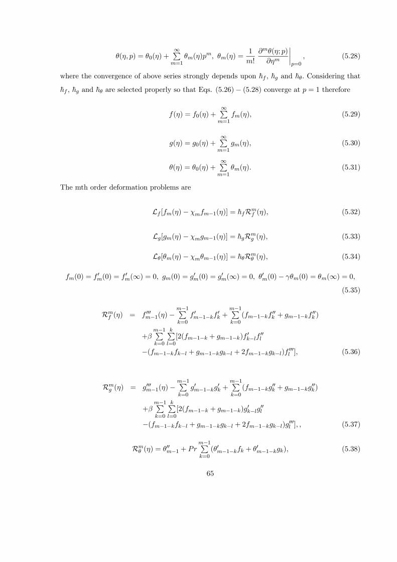
( ) = 0() +∞P
=1
() () =
1
!
(; )
¯=0
(5.28)
where the convergence of above series strongly depends upon ~ ~ and ~ Considering that
~ ~ and ~ are selected properly so that Eqs. (526)− (528) converge at = 1 therefore
() = 0() +∞P
=1
() (5.29)
() = 0() +∞P
=1
() (5.30)
() = 0() +∞P
=1
() (5.31)
The mth order deformation problems are
L [()− −1()] = ~R () (5.32)
L[()− −1()] = ~R () (5.33)
L[()− −1()] = ~R () (5.34)
(0) = 0(0) = 0(∞) = 0 (0) = 0(0) = 0(∞) = 0 0(0)− (0) = (∞) = 0(5.35)
R () = 000−1()−
−1P=0
0−1−0 +
−1P=0
(−1− 00 + −1− 00 )
+−1P=0
P=0
[2(−1− + −1−) 0−00
−(−1−− + −1−− + 2−1−−) 000 ] (5.36)
R () = 000−1()−
−1P=0
0−1−0 +
−1P=0
(−1−00 + −1−00)
+−1P=0
P=0
[2(−1− + −1−)0−00
−(−1−− + −1−− + 2−1−−)000 ] (5.37)
R () = 00−1 +
−1P=0
(0−1− + 0−1−) (5.38)
65
=
⎡⎣ 0 ≤ 11 1
(5.39)
Solving the corresponding mth order deformation problems we have
() = ∗() + 1 + 2 + 3
− (5.40)
() = ∗() + 4 + 5 + 6
− (5.41)
() = ∗() +7 + 8
− (5.42)
in which the ∗ ∗ and ∗ indicate the special solutions.
5.3 Convergence analysis and discussion of results
Obviously the series (529) − (531) consists of the auxiliary parameters ~ ~ and ~. Theseparameters have a key role to adjust and control the convergence of homotopic solutions. The
~−curves have been sketched at 18 order of approximations to determine the suitable rangesfor ~ ~ and ~. From Figs. 5.1 − 53 it is noted that the range of admissible values of~ ~ and ~ are −130 ≤ ~ ≤ −030 −130 ≤ ~ ≤ −025 and −140 ≤ ~ ≤ −045 Weobserved that (see Table 1) that our series solutions converge in the whole region of when
~ = ~ = −090 and ~ = −100 (see Table 5.1).Figs. 5.4-5.16 depict the behaviors of Deborah number Prandtl number and Biot
number on temperature () for different cases when = 00 05 and 10 Variations of
and are shown in the Figs 5.4−56 when = 0 It is seen that an increase in Prandtl number shows a decrease in the temperature of fluid and the thermal boundary layer thickness (see
Fig. 5.4). Figs. 5.5 and 5.6 show the variations of Deborah and Biot numbers. We conclude
from these Figs. that both the temperature profile and thermal boundary layer thickness
increase when Deborah and Biot number increase. It is also noted that the fluid temperature
is zero when the Biot number is zero. The effects of and on temperature are displayed
in the Figs. 5.7− 59 for = 05 The plotted Figs. depict that results for = 0 and = 05
are similar in a qualitative sense. The only change here that we noted is in the variation of
This can be seen by comparing the Figs. 5.5 and 5.8 The variation in temperature for the case
66
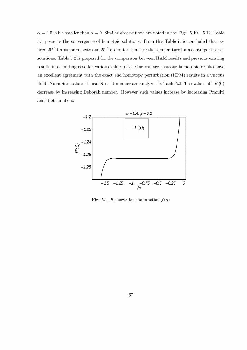
= 05 is bit smaller than = 0 Similar observations are noted in the Figs. 5.10−512 Table5.1 presents the convergence of homotpic solutions. From this Table it is concluded that we
need 20 terms for velocity and 25 order iterations for the temperature for a convergent series
solutions. Table 5.2 is prepared for the comparison between HAM results and previous existing
results in a limiting case for various values of One can see that our homotopic results have
an excellent agreement with the exact and homotopy perturbation (HPM) results in a viscous
fluid. Numerical values of local Nusselt number are analyzed in Table 5.3 The values of −0(0)decrease by increasing Deborah number. However such values increase by increasing Prandtl
and Biot numbers.
-1.5 -1.25 -1 -0.75 -0.5 -0.25 0Ñf
-1.28
-1.26
-1.24
-1.22
-1.2
f''0
a =0.4, b =0.2
f ''0
Fig. 5.1: ~−curve for the function ()
67
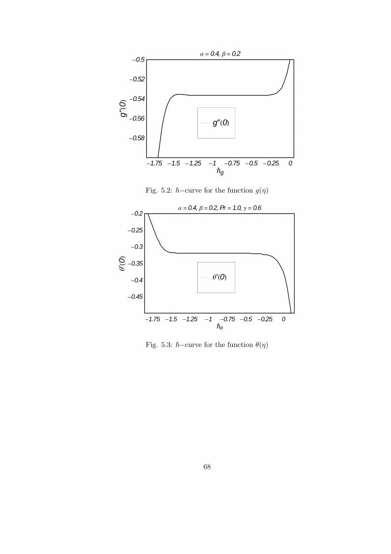
-1.75 -1.5 -1.25 -1 -0.75 -0.5 -0.25 0Ñg
-0.58
-0.56
-0.54
-0.52
-0.5
g''0
a= 0.4, b= 0.2
g''0
Fig. 5.2: ~−curve for the function ()
-1.75 -1.5 -1.25 -1 -0.75 -0.5 -0.25 0Ñq
-0.45
-0.4
-0.35
-0.3
-0.25
-0.2
q'0
a =0.4, b =0.2, Pr = 1.0, g = 0.6
q'0
Fig. 5.3: ~−curve for the function ()
68

0 1 2 3 4 5 6h
0
0.2
0.4
0.6
0.8
1
f'h
a = 0.3
b = 1.0b = 0.7b = 0.4b = 0.0
Fig. 5.4: Influence of on 0()
0 1 2 3 4 5 6h
0
0.2
0.4
0.6
0.8
1
f'h
b = 0.5
a = 1.0a = 0.6a = 0.3a = 0.0
Fig. 5.5: Influence of on 0()
69

0 1 2 3 4 5 6h
0
0.1
0.2
0.3
0.4
0.5
g'h
a = 0.5
b = 1.0b = 0.6b = 0.3b = 0.0
Fig. 5.6: Influence of on 0()
0 1 2 3 4 5 6h
0
0.2
0.4
0.6
0.8
1
g'h
b = 0.5
a = 1.0a = 0.7a = 0.4a = 0.0
Fig. 5.7: Influence of on 0()
70
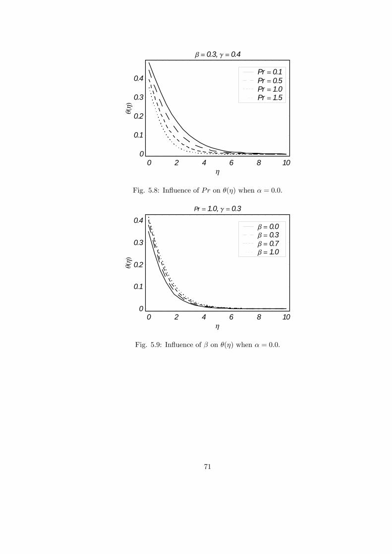
0 2 4 6 8 10h
0
0.1
0.2
0.3
0.4
qh
b = 0.3, g = 0.4
Pr = 1.5Pr = 1.0Pr = 0.5Pr = 0.1
Fig. 5.8: Influence of on () when = 00
0 2 4 6 8 10h
0
0.1
0.2
0.3
0.4
qh
Pr = 1.0, g = 0.3
b = 1.0b = 0.7b = 0.3b = 0.0
Fig. 5.9: Influence of on () when = 00
71

0 2 4 6 8 10h
0
0.1
0.2
0.3
0.4
0.5
qh
Pr = 0.7, b = 0.3
g = 0.6g = 0.4g = 0.2g = 0.0
Fig. 5.10: Influence of on () when = 00
0 2 4 6 8 10h
0
0.1
0.2
0.3
0.4
qh
b = 0.3, g = 0.4
Pr = 1.5Pr = 1.0Pr = 0.5Pr = 0.1
Fig. 5.11: Influence of on () when = 05
72
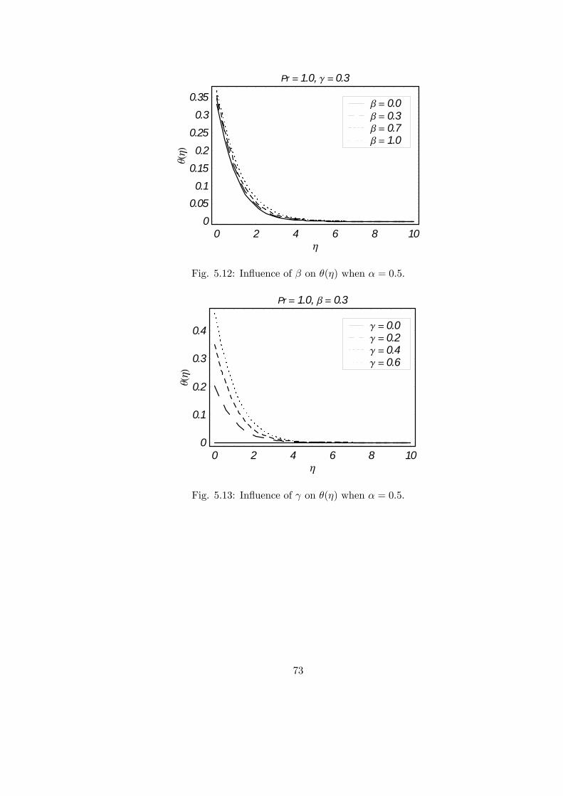
0 2 4 6 8 10h
0
0.05
0.1
0.15
0.2
0.25
0.3
0.35
qh
Pr = 1.0, g = 0.3
b = 1.0b = 0.7b = 0.3b = 0.0
Fig. 5.12: Influence of on () when = 05
0 2 4 6 8 10h
0
0.1
0.2
0.3
0.4
qh
Pr = 1.0, b = 0.3
g = 0.6g = 0.4g = 0.2g = 0.0
Fig. 5.13: Influence of on () when = 05
73
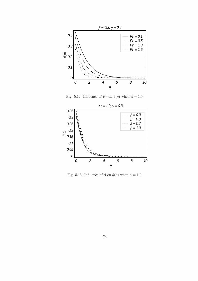
0 2 4 6 8 10h
0
0.1
0.2
0.3
0.4
qh
b = 0.3, g = 0.4
Pr = 1.5Pr = 1.0Pr = 0.5Pr = 0.1
Fig. 5.14: Influence of on () when = 10
0 2 4 6 8 10h
0
0.05
0.1
0.15
0.2
0.25
0.3
0.35
qh
Pr = 1.0, g = 0.3
b = 1.0b = 0.7b = 0.3b = 0.0
Fig. 5.15: Influence of on () when = 10
74
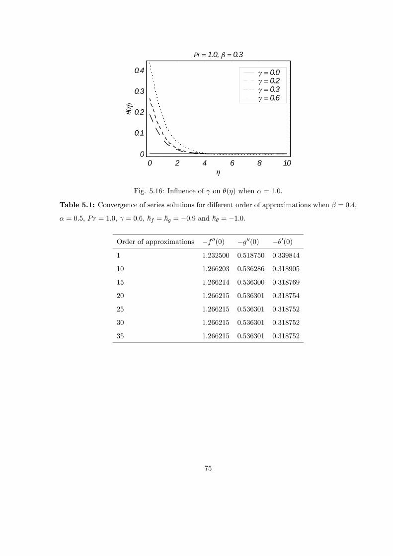
0 2 4 6 8 10h
0
0.1
0.2
0.3
0.4
qh
Pr = 1.0, b = 0.3
g = 0.6g = 0.3g = 0.2g = 0.0
Fig. 5.16: Influence of on () when = 10
Table 5.1: Convergence of series solutions for different order of approximations when = 04
= 05 = 10 = 06 ~ = ~ = −09 and ~ = −10
Order of approximations − 00(0) −00(0) −0(0)1 1.232500 0.518750 0.339844
10 1.266203 0.536286 0.318905
15 1.266214 0.536300 0.318769
20 1.266215 0.536301 0.318754
25 1.266215 0.536301 0.318752
30 1.266215 0.536301 0.318752
35 1.266215 0.536301 0.318752
75
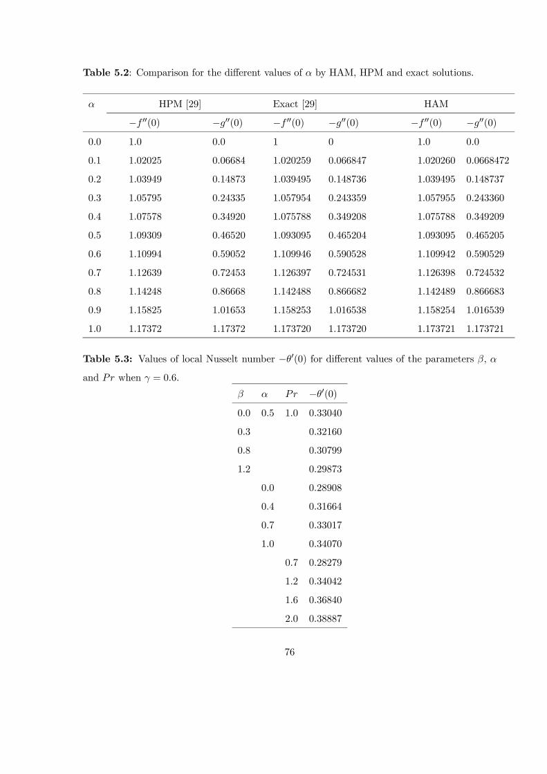
Table 5.2: Comparison for the different values of by HAM, HPM and exact solutions.
HPM [29] Exact [29] HAM
− 00(0) −00(0) − 00(0) −00(0) − 00(0) −00(0)0.0 1.0 0.0 1 0 1.0 0.0
0.1 1.02025 0.06684 1.020259 0.066847 1.020260 0.0668472
0.2 1.03949 0.14873 1.039495 0.148736 1.039495 0.148737
0.3 1.05795 0.24335 1.057954 0.243359 1.057955 0.243360
0.4 1.07578 0.34920 1.075788 0.349208 1.075788 0.349209
0.5 1.09309 0.46520 1.093095 0.465204 1.093095 0.465205
0.6 1.10994 0.59052 1.109946 0.590528 1.109942 0.590529
0.7 1.12639 0.72453 1.126397 0.724531 1.126398 0.724532
0.8 1.14248 0.86668 1.142488 0.866682 1.142489 0.866683
0.9 1.15825 1.01653 1.158253 1.016538 1.158254 1.016539
1.0 1.17372 1.17372 1.173720 1.173720 1.173721 1.173721
Table 5.3: Values of local Nusselt number −0(0) for different values of the parameters and when = 06.
−0(0)0.0 0.5 1.0 0.33040
0.3 0.32160
0.8 0.30799
1.2 0.29873
0.0 0.28908
0.4 0.31664
0.7 0.33017
1.0 0.34070
0.7 0.28279
1.2 0.34042
1.6 0.36840
2.0 0.38887
76
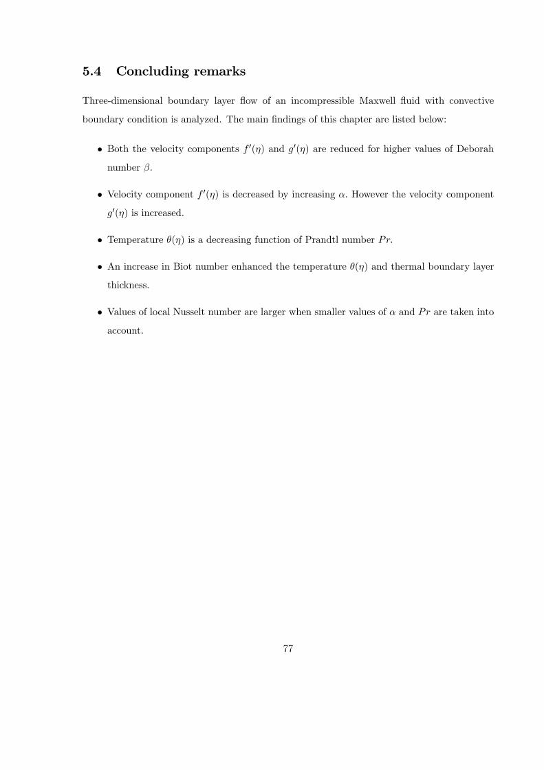
5.4 Concluding remarks
Three-dimensional boundary layer flow of an incompressible Maxwell fluid with convective
boundary condition is analyzed. The main findings of this chapter are listed below:
• Both the velocity components 0() and 0() are reduced for higher values of Deborah
number
• Velocity component 0() is decreased by increasing However the velocity component0() is increased.
• Temperature () is a decreasing function of Prandtl number
• An increase in Biot number enhanced the temperature () and thermal boundary layerthickness.
• Values of local Nusselt number are larger when smaller values of and are taken intoaccount.
77
Chapter 6
MHD three-dimensional flow of
Maxwell fluid with variable thermal
conductivity and heat source/sink
This chapter investigates the effects of applied magnetic field and heat transfer in flow of
Maxwell fluid with variable thermal conductivity. Three dimensional flow is induced by a
stretching surface. The thermal conductivity is taken temperature dependent. Heat transfer
analysis is carried out in the presence of heat source/sink. The series solutions are constructed
and results are interpreted through the effects of various embedded parameters. Comparison
with the previous limiting solutions is shown in an excellent agreement.
6.1 Mathematical formulation of the problems
A steady three-dimensional laminar flow of an incompressible Maxwell fluid (with variable
thermal conductivity) past a stretching surface is considered. A constant magnetic field of
strength B0 is applied. Induced magnetic field is not accounted. In addition concept of heat
source/sink in heat transfer analysis is considered. The thermal conductivity depends upon
temperature. The boundary layer assumptions are utilized in problems formulation. Thus the
78

governing equations for present flow configuration are reduced into the following equations:
+
+
= 0 (6.1)
+
+
=
2
2− 1
⎛⎝ 2 2
2+ 2
22
+ 2 22
+ 2 2
+2 2
+ 2 2
⎞⎠−
∗20
µ+ 1
¶ (6.2)
+
+
=
2
2− 1
⎛⎝ 2 2
2+ 2
22
+ 2 2
2+ 2 2
+
2 2
+ 2 2
⎞⎠−
∗20
µ + 1
¶ (6.3)
µ
+
+
¶=
µ
¶+( − ∞) (6.4)
Here the respective velocity components in the − − and −directions are represented by and , 1 the relaxation time, the fluid temperature, the variable thermal conductivity
of the fluid, = () the kinematic viscosity, the dynamic viscosity, the density, the
electrical conductivity, the specific heat and the heat source/sink parameter with 0
(heat source) and 0 (heat sink).
The boundary conditions associated to the flow consideration are
= () = = () = = 0 = at = 0 (6.5)
→ 0 → 0 → ∞ when →∞ (6.6)
in which variable thermal conductivity is
= ∞(1 + ) = − ∞
∞ (6.7)
where ∞ represents the fluid free stream conductivity and the conductivity at the wall.
79
We now employ the following transformations
= 0() = 0() = −√(() + ()) () = − ∞ − ∞
=
r
(6.8)
Now Eq. (6.1) is obviously satisfied and Eqs. (62) − (67) are presented into the followingforms:
000 + (2 + 1)( + ) 00 − 02 + ¡2( + ) 0 00 − ( + )2 000
¢−2 0 = 0 (6.9)
000 + (2 + 1)( + )00 − 02 + ¡2( + )000 − ( + )2000
¢−20 = 0 (6.10)
(1 + )00 + ( + )0 + 02 + = 0 (6.11)
= 0 = 0 0 = 1 0 = = 1 at = 0 (6.12)
0 → 0 0 → 0 → 0 as →∞ (6.13)
in which the parameters entering into above equations are (= 1) the Deborah number
(= ) the ratio of stretching rates, =
20
the Hartman number, ¡=
¢the Prandtl
number, ³=
´the heat source/sink parameter and prime the differentiation with respect
to
Local Nusselt number with heat transfer has the following definition
=
( − ∞) = −
µ
¶=0
(6.14)
Dimensionless expression of local Nusselt number is
12 = −0(0) (6.15)
where (= ) is the local Reynolds number.
80
6.2 Solutions
The initial guesses and auxiliary linear operators for the homotopy solutions can be expressed
in the forms:
0() = 1− exp(−) 0() = (1− exp(−)) 0() = exp(−) (6.16)
L = 000 − 0 L = 000 − 0 L = 00 − (6.17)
in which
L (1 + 2 + 3
−) = 0 L(4 + 5 + 6
−) = 0 L(7 + 8−) = 0 (6.18)
and ( = 1− 8) denote the arbitrary constants.The corresponding zeroth order problems are
(1− )Lh(; )− 0()
i= ~N
h(; ) (; )
i (6.19)
(1− )L [(; )− 0()] = ~N
h(; ) (; )
i (6.20)
(1− )Lh(; )− 0()
i= ~N
h(; ) (; ) ( )
i (6.21)
(0; ) = 0 0(0; ) = 1 0(∞; ) = 0 (0; ) = 0 0(0; ) = 0(∞; ) = 0
0(0 ) = (∞ ) = 0 (6.22)
N [( ) ( )] =3( )
3−Ã( )
!2+ (2 + 1)(( ) + ( ))
2( )
2
+
⎛⎝ 2(( ) + ( ))()
2()
2
−(( ) + ( ))23()
2
⎞⎠−2( )
(6.23)
81
N[( ) ( )] =3( )
3−µ( )
¶2+ (2 + 1)(( ) + ( ))
2( )
2
+
⎛⎝ 2(( ) + ( ))()
2()
2
−(( ) + ( ))23()
2
⎞⎠−2( )
(6.24)
N[( ) ( ) ( )] =³1 + ( )
´ 2( )
2+Pr(( ) + ( ))
( )
+
Ã( )
!2 (6.25)
where is an embedding parameter, ~ ~ and ~ the non-zero auxiliary parameters and N
N and N the nonlinear operators. When = 0 and = 1 then
(; 0) = 0() ( 0) = 0() and (; 1) = () ( 1) = () (6.26)
We notice that when increases from 0 to 1 then ( ) ( ) and ( ) vary from 0()
0() 0() to () () and () Using Taylor’s expansion we get
( ) = 0() +∞P
=1
() () =
1
!
(; )
¯=0
(6.27)
( ) = 0() +∞P
=1
() () =
1
!
(; )
¯=0
(6.28)
( ) = 0() + ∞P
=1
() () =
1
!
(; )
¯=0
(6.29)
where the convergence of series strongly depends upon ~ ~ and ~ Considering that ~ ~
and ~ are selected properly so that Eqs. (626)− (628) converge at = 1 Hence
() = 0() +∞P
=1
() (6.30)
() = 0() +∞P
=1
() (6.31)
() = 0() +∞P
=1
() (6.32)
82
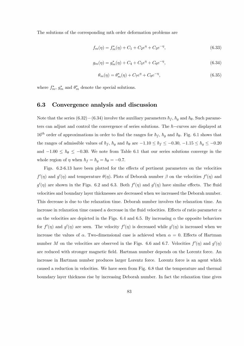
The solutions of the corresponding mth order deformation problems are
() = ∗() + 1 + 2 + 3
− (6.33)
() = ∗() + 4 + 5 + 6
− (6.34)
() = ∗() +7 + 8
− (6.35)
where ∗ ∗ and ∗ denote the special solutions.
6.3 Convergence analysis and discussion
Note that the series (632)−(634) involve the auxiliary parameters ~ ~ and ~ Such parame-ters can adjust and control the convergence of series solutions. The ~−curves are displayed at16 order of approximations in order to find the ranges for ~ ~ and ~. Fig. 6.1 shows that
the ranges of admissible values of ~ ~ and ~ are −110 ≤ ~ ≤ −030 −115 ≤ ~ ≤ −020and −100 ≤ ~ ≤ −030 We note from Table 6.1 that our series solutions converge in the
whole region of when ~ = ~ = ~ = −07Figs. 6.2-6.13 have been plotted for the effects of pertinent parameters on the velocities
0() and 0() and temperature () Plots of Deborah number on the velocities 0() and
0() are shown in the Figs. 6.2 and 6.3. Both 0() and 0() have similar effects. The fluid
velocities and boundary layer thicknesses are decreased when we increased the Deborah number.
This decrease is due to the relaxation time. Deborah number involves the relaxation time. An
increase in relaxation time caused a decrease in the fluid velocities. Effects of ratio parameter
on the velocities are depicted in the Figs. 6.4 and 6.5. By increasing the opposite behaviors
for 0() and 0() are seen. The velocity 0() is decreased while 0() is increased when we
increase the values of Two-dimensional case is achieved when = 0 Effects of Hartman
number on the velocities are observed in the Figs. 6.6 and 6.7. Velocities 0() and 0()
are reduced with stronger magnetic field. Hartman number depends on the Lorentz force. An
increase in Hartman number produces larger Lorentz force. Lorentz force is an agent which
caused a reduction in velocities. We have seen from Fig. 6.8 that the temperature and thermal
boundary layer thickness rise by increasing Deborah number. In fact the relaxation time gives
83
rise to the temperature and thermal boundary layer thickness. It is also found that the effects
of Deborah number on the velocities and temperature are reversed. Effects of ratio parameter
on the temperature are analyzed in Fig. 6.9. The temperature and thermal boundary
layer thickness are decreasing functions of An increase in corresponds to a decrease in
temperature. From Fig. 6.10 we observed that larger values of Prandtl number lead to lower
the temperature and thermal boundary layer thickness. This occurs due to a decrease in thermal
diffusivity. Increase in Prandtl number implies lower thermal diffusivity and smaller thermal
diffusivity shows lower temperature. Fig. 6.11 illustrates that larger values of Hartman number
corresponds to increase in temperature and thermal boundary layer thickness. Fig. 6.12 shows
the behavior of on temperature () The temperature becomes stronger for the larger values
of Fig. 6.13 clearly indicates that heat source/sink parameter gives rise to the temperature
and thermal boundary layer thickness. Table 6.1 provides the convergence values of series
solutions of velocities and temperature. This Table indicates that we need less approximations
for velocities in comparison to the temperature. Table 6.2 is computed just to compare the
analysis with the previous results in a limiting sense for various values of It is found that our
homotopic solutions have an excellent agreement with the previous results for different values
of
-1.5 -1.25 -1 -0.75 -0.5 -0.25 0Ñf , Ñg, Ñq
-1.4
-1.2
-1
-0.8
-0.6
-0.4
-0.2
f''0
,g
''0,q
'0
b =0.4, S= 0.2, M= 0.7, Pr = 1.5, a =0.5, e = 0.3
q'0g''0f''0
84

Fig. 6.1: ~−curves for the functions () () and ()
2 4 6 8 10h
0.2
0.4
0.6
0.8
1
f'h
b = 0.0, 0.2, 0.4, 0.6, 0.8
Fig. 6.2: Influence of on the velocity 0() when = 06 and = 07
2 4 6 8 10h
0.1
0.2
0.3
0.4
0.5
0.6
g'h
b =0.0, 0.2, 0.4, 0.6,0.8
85

Fig. 6.3: Influence of on the velocity 0() when = 06 and = 07
2 4 6 8 10h
0.2
0.4
0.6
0.8
1
f'h
a= 0.1, 0.3, 0.5, 0.7, 1.0
Fig. 6.4: Influence of on the velocity 0() when = 03 and = 07
2 4 6 8 10h
0.2
0.4
0.6
0.8
1
g'h
a= 0.1, 0.3, 0.6, 0.8, 1.0
86
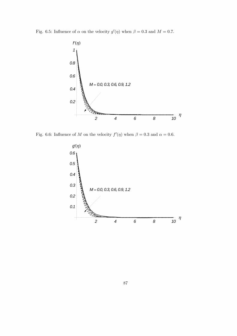
Fig. 6.5: Influence of on the velocity 0() when = 03 and = 07
2 4 6 8 10h
0.2
0.4
0.6
0.8
1
f'h
M= 0.0, 0.3, 0.6, 0.9, 1.2
Fig. 6.6: Influence of on the velocity 0() when = 03 and = 06
2 4 6 8 10h
0.1
0.2
0.3
0.4
0.5
0.6
g'h
M=0.0, 0.3, 0.6, 0.9, 1.2
87

Fig. 6.7: Influence of on the velocity 0() when = 03 and = 06
2 4 6 8 10h
0.2
0.4
0.6
0.8
1
qh
b =0.0, 0.2, 0.4, 0.6, 0.8
Fig. 6.8: Influence of on the temperature () when = 06 = 07 = 12 = 02
and = 03
2 4 6 8 10h
0.2
0.4
0.6
0.8
1
qh
a =0.1, 0.3, 0.5, 0.7, 1.0
Fig. 6.9: Influence of on the temperature () when = 03 = 07 = 12 = 02
88
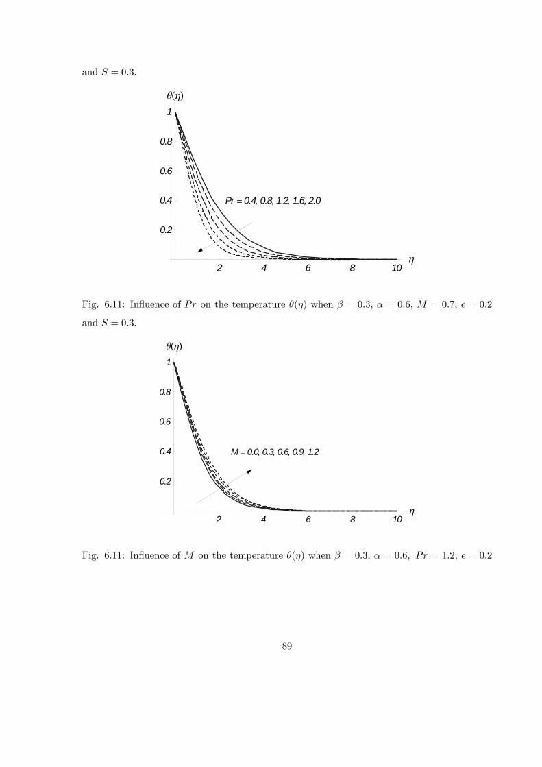
and = 03
2 4 6 8 10h
0.2
0.4
0.6
0.8
1
qh
Pr =0.4, 0.8, 1.2, 1.6, 2.0
Fig. 6.11: Influence of on the temperature () when = 03 = 06 = 07 = 02
and = 03
2 4 6 8 10h
0.2
0.4
0.6
0.8
1
qh
M= 0.0, 0.3, 0.6, 0.9, 1.2
Fig. 6.11: Influence of on the temperature () when = 03 = 06 = 12 = 02
89
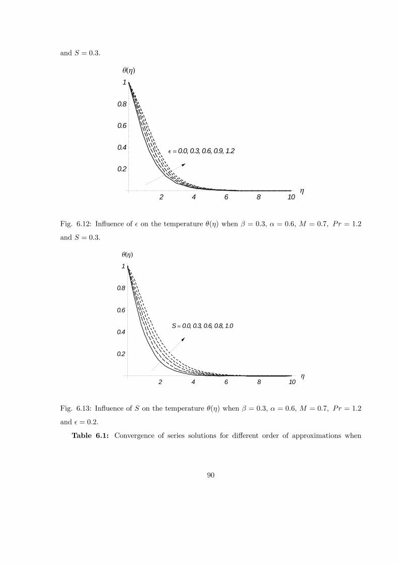
and = 03
2 4 6 8 10h
0.2
0.4
0.6
0.8
1
qh
e =0.0, 0.3, 0.6, 0.9, 1.2
Fig. 6.12: Influence of on the temperature () when = 03 = 06 = 07 = 12
and = 03
2 4 6 8 10h
0.2
0.4
0.6
0.8
1
qh
S= 0.0, 0.3, 0.6, 0.8, 1.0
Fig. 6.13: Influence of on the temperature () when = 03 = 06 = 07 = 12
and = 02
Table 6.1: Convergence of series solutions for different order of approximations when
90

= 03 = 05 = 07 = 15 = 03, = 02 and ~ = ~ = ~ = −07
Order of approximations − 00(0) −00(0) −0(0)1 1.386633 0.617483 0.66750
5 1.477280 0.658060 0.50817
15 1.477327 0.658282 0.47558
20 1.477328 0.658282 0.47349
25 1.477328 0.658282 0.47242
30 1.477328 0.658282 0.47242
40 1.477328 0.658282 0.47242
Table 6.2: Comparison for different values of by HAM, HPM and exact solutions.
[29] [25] Present solutions
− 00(0) −00(0) − 00(0) −00(0) − 00(0) −00(0)0.0 1.0 0.0 1.0 0 1.0 0.0
0.10 1.02025 0.06684 – – 1.020260 0.0668472
0.20 1.03949 0.14873 – – 1.039495 0.148737
0.25 – – 1.048813 0.194564 1.04881 0.19457
0.30 1.05795 0.24335 – – 1.057955 0.243360
0.40 1.07578 0.34920 – – 1.075788 0.349209
0.50 1.09309 0.46520 1.093097 0.465205 1.093095 0.465205
0.60 1.10994 0.59052 – – 1.109942 0.590529
0.70 1.12639 0.72453 – – 1.126398 0.724532
0.75 – – 1.134485 0.794622 1.13450 0.79462
0.80 1.14248 0.86668 – – 1.142489 0.866683
0.90 1.15825 1.01653 – – 1.158254 1.016539
1.00 1.17372 1.17372 1.173720 1.173720 1.173721 1.173721
91
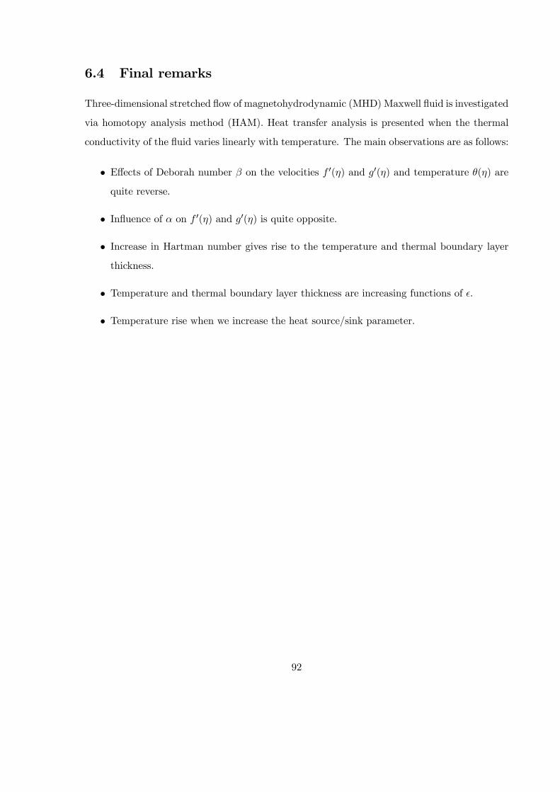
6.4 Final remarks
Three-dimensional stretched flow of magnetohydrodynamic (MHD) Maxwell fluid is investigated
via homotopy analysis method (HAM). Heat transfer analysis is presented when the thermal
conductivity of the fluid varies linearly with temperature. The main observations are as follows:
• Effects of Deborah number on the velocities 0() and 0() and temperature () are
quite reverse.
• Influence of on 0() and 0() is quite opposite.
• Increase in Hartman number gives rise to the temperature and thermal boundary layerthickness.
• Temperature and thermal boundary layer thickness are increasing functions of
• Temperature rise when we increase the heat source/sink parameter.
92
Chapter 7
Hydromagnetic steady flow of
Maxwell fluid over a bidirectional
stretching surface with prescribed
surface temperature and prescribed
surface heat flux
This chapter investigates the effects of heat transfer in steady hydromagnetic three-dimensional
boundary layer flow of Maxwell fluid by a bidirectional stretching surface. Two cases are
considered. Explicitly heat transfer process is analyzed due to prescribed surface temperature
(PST) and prescribed heat flux (PHF). Results are plotted and examined. Convergence for
the solutions is presented for the temperatures. Comparison of PST and PHF cases with the
existing solutions in a limiting sense is given and illustrated.
93
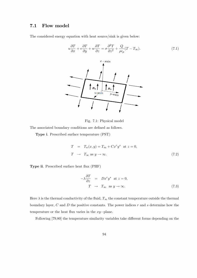
7.1 Flow model
The considered energy equation with heat source/sink is given below:
+
+
=
2
2+
( − ∞) (7.1)
Fig. 7.1: Physical model
The associated boundary conditions are defined as follows.
Type i. Prescribed surface temperature (PST)
= ( ) = ∞ + at = 0
→ ∞ as →∞ (7.2)
Type ii. Prescribed surface heat flux (PHF)
−
= at = 0
→ ∞ as →∞ (7.3)
Here is the thermal conductivity of the fluid, ∞ the constant temperature outside the thermal
boundary layer, and the positive constants. The power indices and determine how the
temperature or the heat flux varies in the −plane.Following [79,80] the temperature similarity variables take different forms depending on the
94
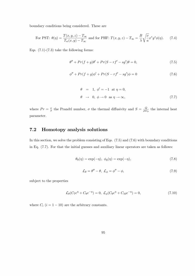
boundary conditions being considered. These are
For PST: () = ( )− ∞( )− ∞
and for PHF: ( )− ∞ =
r
() (7.4)
Eqs. (7.1)-(7.3) take the following forms:
00 + ( + )0 + ( − 0 − 0) = 0 (7.5)
00 + ( + )0 + ( − 0 − 0) = 0 (7.6)
= 1 0 = −1 at = 0
→ 0 → 0 as →∞ (7.7)
where = the Prandtl number, the thermal diffusivity and =
the internal heat
parameter.
7.2 Homotopy analysis solutions
In this section, we solve the problem consisting of Eqs. (7.5) and (7.6) with boundary conditions
in Eq. (7.7). For that the initial guesses and auxiliary linear operators are taken as follows:
0() = exp(−) 0() = exp(−) (7.8)
L = 00 − L = 00 − (7.9)
subject to the properties
L(7 + 8−) = 0 L(9 + 10
−) = 0 (7.10)
where ( = 1− 10) are the arbitrary constants.
95
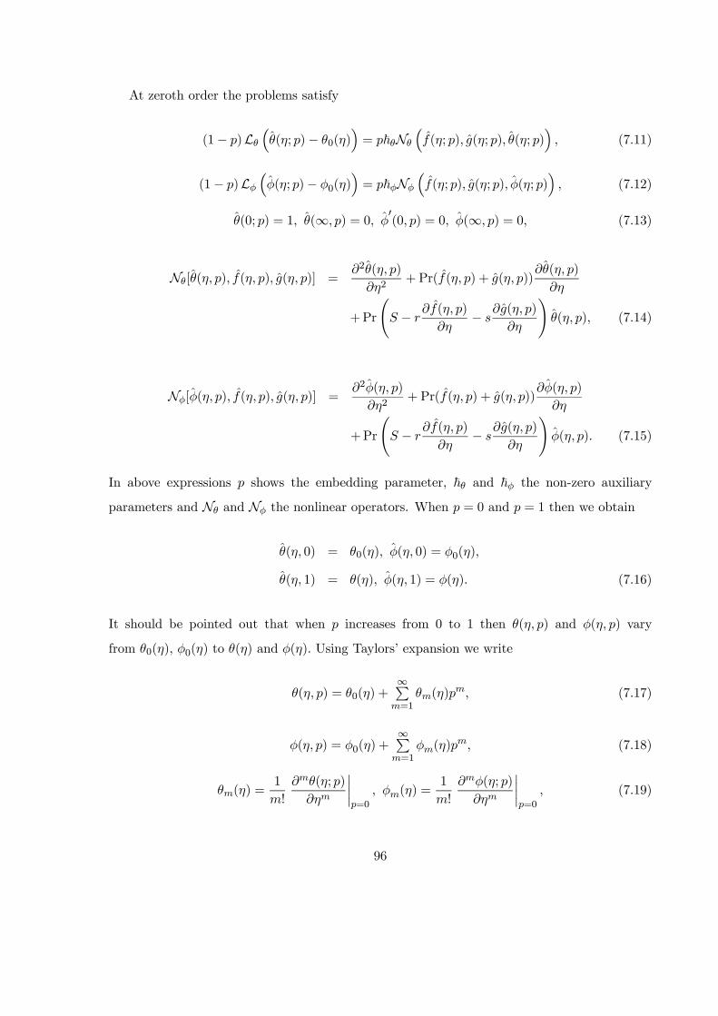
At zeroth order the problems satisfy
(1− )L³(; )− 0()
´= ~N
³(; ) (; ) (; )
´ (7.11)
(1− )L³(; )− 0()
´= ~N
³(; ) (; ) (; )
´ (7.12)
(0; ) = 1 (∞ ) = 0 0(0 ) = 0 (∞ ) = 0 (7.13)
N[( ) ( ) ( )] =2( )
2+Pr(( ) + ( ))
( )
+Pr
à −
( )
−
( )
!( ) (7.14)
N[( ) ( ) ( )] =2( )
2+Pr(( ) + ( ))
( )
+Pr
à −
( )
−
( )
!( ) (7.15)
In above expressions shows the embedding parameter, ~ and ~ the non-zero auxiliary
parameters and N and N the nonlinear operators. When = 0 and = 1 then we obtain
( 0) = 0() ( 0) = 0()
( 1) = () ( 1) = () (7.16)
It should be pointed out that when increases from 0 to 1 then ( ) and ( ) vary
from 0() 0() to () and () Using Taylors’ expansion we write
( ) = 0() +∞P
=1
() (7.17)
( ) = 0() +∞P
=1
() (7.18)
() =1
!
(; )
¯=0
() =1
!
(; )
¯=0
(7.19)
96

where the parameters ~ and ~ have a key role in the convergence of series solutions. The
values of parameters are chosen in such a manner that Eqs. (719) and (720) converge at = 1
Hence Eqs. (719) and (720) give
() = 0() +∞P
=1
() (7.20)
() = 0() +∞P
=1
() (7.21)
The general solutions are arranged as follows.
() = ∗() +7 + 8
− (7.22)
() = ∗() + 9 + 10
− (7.23)
in which the special solutions are denoted by ∗ and ∗
7.3 Convergence of series solutions and discussion
It is well known fact that the homotopy analysis method has a great freedom to choose the
auxiliary parameters ~ and ~ for adjusting and controlling the convergence of series solu-
tions. To determine the appropriate convergence interval of the constructed series solutions,
the ~−curves at 17-order of approximations are sketched. Figs. 7.1 and 7.2 clearly show thatthe range of admissible values of ~ and ~ are −140 ≤ ~ ≤ −04 and −135 ≤ ~ ≤ −025
The results are displayed graphically to see the effects of and on
the prescribed surface temperature and prescribed surface heat flux. We denote temperature
variation for PST case by () and for PHF situation by () in the Figs. 7.3-7.16. Figs. 7.3
and 7.4 illustrate the variations of Deborah number on () and () From these Figs. we have
seen that both () and () are increased with an increase in Deborah number is based
on the relaxation time. When Deborah number increases then relaxation time increases. This
increase in relaxation time causes an increase in () and () Comparison of Figs. 7.3 and 7.4
show that has similar effects on () and () Figs. 7.5 and 7.6 are plotted to see the effects
of magnetic parameter on () and () Clearly the thermal boundary layer thicknesses
97

are increased for larger values of magnetic parameter. In fact the magnetic parameter involves
the Lorentz force. Larger values of magnetic parameter corresponds to the stronger Lorentz
force. This stronger Lorentz force give rise to the thermal boundary layer thicknesses. Figs.
7.7 and 7.8 illustrate the variations of on () and () From these Figs. it is noticed
that both () and () are reduced when we increased the values of Also the thermal
boundary layer becomes thinner for higher values of This reduction in thermal boundary
layer for larger values of is due to the entertainment of cooler to ambient fluid. The power
indices and control the non-uniformity of the surface temperature in the prescribed surface
temperature situation. Figs. 7.9 and 7.10 depict that () and () are decreasing functions
of Also we noted that () reduces rapidly in comparison to () Effect of on () and
() are seen in the Figs. 7.11 and 7.12. The values of () and () are reduced when
values of are increased. It is concluded that the non-uniformity of the sheet temperature
has prominent effect on the temperature fields for the reduction in temperature and thinner
thermal boundary layer. Comparison of Figs. 7.11 and 7.12 illustrates that the variations in
() are more pronounced when compared to the variations in () Also we examined that ()
at the wall is reduced rapidly when the values of are larger. Figs. 7.13 and 7.14 depict the
variations of heat generation/absorption parameter on () and () Both () and () are
increased by increasing values of heat generation/absorption parameter. Physically an increase
in heat generation/absorption parameter produced more heat due to which the temperature of
fluid increases. Such increase in temperature gives rise to () and () The effects of Prandtl
number on () and () are analyzed in the Figs. 7.15 and 7.16. These Figs. clearly show that
() () and their related thermal boundary layer thicknesses are reduced for the larger values
of Prandtl number Obviously the Prandtl number depends upon the thermal diffusivity.
Larger values of Prandtl number give smaller thermal diffusivity and consequently the values
of () and () decrease.
Table 7.1 has been prepared to analyze the convergent values of () and () We have
seen that our solutions for velocities converge from 16th order of approximations whereas one
needs 25th order of deformations for () and () Hence we need less deformations for the
velocities in comparison to temperatures for a convergent solution. Table 7.2 provides the values
of temperature gradient 0(0) for different values of and when = = 0 and = 10
98
One can see that our solutions has an excellent agreement with the previous results in a limiting
case. Further it is observed that the temperature gradient at surface 0(0) becomes positive and
it reduces for = −20 and = 0 and negative for = 0 and = −20 Table 7.3 presents thenumerical values of 0(0) and (0) for different values of and when = = 0 = = 10
and = 025 From this Table we noted that our series solutions have very good agreement
with the previous available results in the literature.
-1.5 -1.25 -1 -0.75 -0.5 -0.25 0Ñq
-1.4
-1.2
-1
-0.8
-0.6
q'0
q'0
Fig. 7.1: ~−curve for the function () when = 01 = 07 = 05 = 14 = = 04
and = 03
-1.5 -1.25 -1 -0.75 -0.5 -0.25 0Ñf
0
0.2
0.4
0.6
0.8
1
f''0
f''0
99

Fig. 7.2: ~−curve for the function () when = 01 = 07 = 05 = 14 = = 04
and = 03
2 4 6 8h
0.2
0.4
0.6
0.8
1
qh
b = 0.0, 0.3, 0.6, 1.0, 1.4
Fig. 7.3: Influence of on () when = 07 = 05 = 15 = 03 = 04 and = 04
2 4 6 8h
0.25
0.5
0.75
1
1.25
1.5
fh
b = 0.0, 0.3, 0.6, 1.0, 1.4
100
Fig. 7.4: Influence of on () when = 07 = 05 = 15 = 03 = 04 and = 04
2 4 6 8h
0.2
0.4
0.6
0.8
1
qh
M=0.0, 0.4, 0.8, 1.2, 1.6
Fig. 7.5: Influence of on () when = 02 = 05 = 15 = 03 = 04 and = 04
2 4 6 8h
0.2
0.4
0.6
0.8
1
1.2
fh
M=0.0, 0.4, 0.8, 1.2, 1.6
101
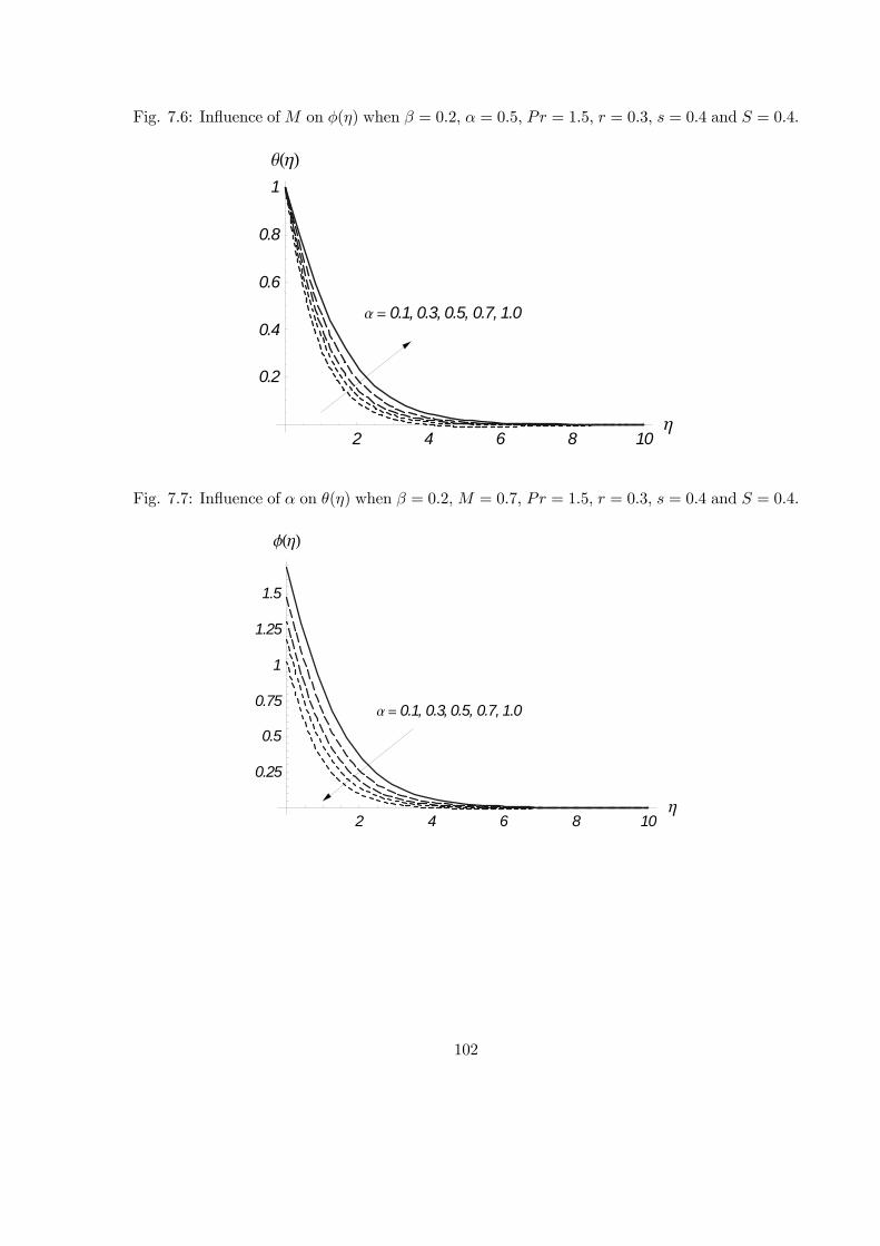
Fig. 7.6: Influence of on () when = 02 = 05 = 15 = 03 = 04 and = 04
2 4 6 8 10h
0.2
0.4
0.6
0.8
1
qh
a= 0.1, 0.3, 0.5, 0.7, 1.0
Fig. 7.7: Influence of on () when = 02 = 07 = 15 = 03 = 04 and = 04
2 4 6 8 10h
0.25
0.5
0.75
1
1.25
1.5
fh
a= 0.1, 0.3, 0.5, 0.7, 1.0
102

Fig. 7.8: Influence of on () when = 02 = 07 = 15 = 03 = 04 and = 04
2 4 6 8h
0.2
0.4
0.6
0.8
1
qh
s=0.0, 0.6, 1.2, 1.8, 2.5
Fig. 7.9: Influence of on () when = 02 = 07 = 15 = 03 = 05 and = 04
2 4 6 8h
0.2
0.4
0.6
0.8
1
1.2
1.4
fh
s=0.0, 0.6, 1.2, 1.8, 2.5
Fig. 7.10: Influence of on () when = 02 = 07 = 15 = 03 = 05 and
103

= 04
2 4 6 8h
0.2
0.4
0.6
0.8
1
qh
r = 0.0, 0.6, 1.2, 1.8, 2.5
Fig. 7.11: Influence of on () when = 02 = 07 = 15 = 04 = 05 and
= 04
2 4 6 8h
0.25
0.5
0.75
1
1.25
1.5
fh
r =0.0, 0.6, 1.2, 1.8, 2.5
Fig. 7.12: Influence of on () when = 02 = 07 = 15 = 04 = 05 and
104
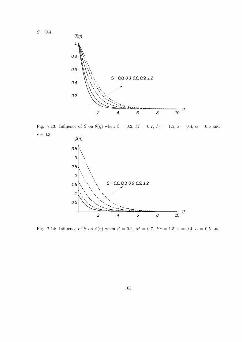
= 04
2 4 6 8 10h
0.2
0.4
0.6
0.8
1
qh
S= 0.0, 0.3, 0.6, 0.9, 1.2
Fig. 7.13: Influence of on () when = 02 = 07 = 15 = 04 = 05 and
= 03
2 4 6 8 10h
0.5
1
1.5
2
2.5
3
3.5
fh
S= 0.0, 0.3, 0.6, 0.9, 1.2
Fig. 7.14: Influence of on () when = 02 = 07 = 15 = 04 = 05 and
105
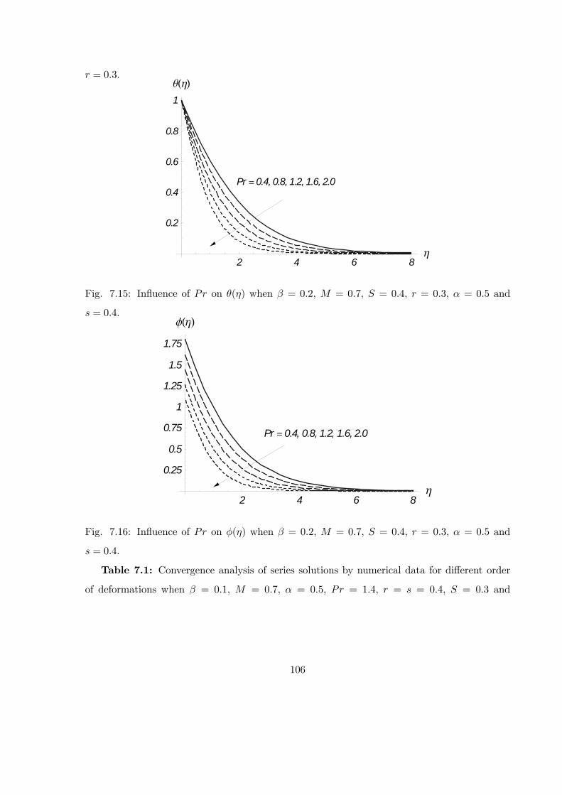
= 03
2 4 6 8h
0.2
0.4
0.6
0.8
1
qh
Pr =0.4, 0.8, 1.2, 1.6, 2.0
Fig. 7.15: Influence of on () when = 02 = 07 = 04 = 03 = 05 and
= 04
2 4 6 8h
0.25
0.5
0.75
1
1.25
1.5
1.75
fh
Pr =0.4, 0.8, 1.2, 1.6, 2.0
Fig. 7.16: Influence of on () when = 02 = 07 = 04 = 03 = 05 and
= 04
Table 7.1: Convergence analysis of series solutions by numerical data for different order
of deformations when = 01 = 07 = 05 = 14 = = 04 = 03 and
106
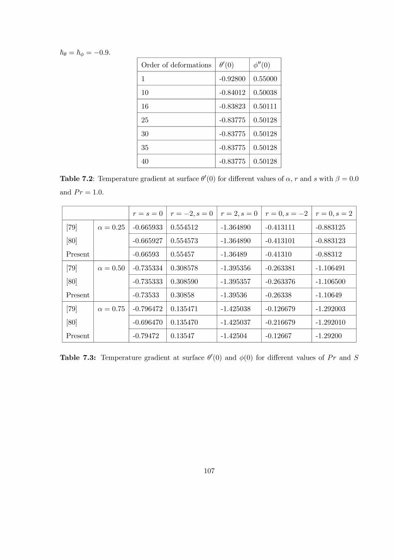
~ = ~ = −09Order of deformations 0(0) 00(0)
1 -0.92800 0.55000
10 -0.84012 0.50038
16 -0.83823 0.50111
25 -0.83775 0.50128
30 -0.83775 0.50128
35 -0.83775 0.50128
40 -0.83775 0.50128
Table 7.2: Temperature gradient at surface 0(0) for different values of and with = 00
and = 10
= = 0 = −2 = 0 = 2 = 0 = 0 = −2 = 0 = 2
[79] = 025 -0.665933 0.554512 -1.364890 -0.413111 -0.883125
[80] -0.665927 0.554573 -1.364890 -0.413101 -0.883123
Present -0.66593 0.55457 -1.36489 -0.41310 -0.88312
[79] = 050 -0.735334 0.308578 -1.395356 -0.263381 -1.106491
[80] -0.735333 0.308590 -1.395357 -0.263376 -1.106500
Present -0.73533 0.30858 -1.39536 -0.26338 -1.10649
[79] = 075 -0.796472 0.135471 -1.425038 -0.126679 -1.292003
[80] -0.696470 0.135470 -1.425037 -0.216679 -1.292010
Present -0.79472 0.13547 -1.42504 -0.12667 -1.29200
Table 7.3: Temperature gradient at surface 0(0) and (0) for different values of and
107

when = = 0 = = 10 and = 05
0(0) for PST (0) for PHF
= −02 = 00 = 02 = −02 = 00 = 02
Ref. [79] = 10 -1.348064 -1.255781 -1.148932 0.741805 0.796317 0.870355
Ref. [80] -1.348064 -1.255780 -1.148934 0.741808 0.796318 0.870372
Present -1.34806 -1.25578 -1.14893 0.74180 0.76632 0.87037
Ref. [79] = 50 -3.330392 -3.170979 -3.002380 0.300265 0.315360 0.333069
Ref. [80] -3.330394 -3.170981 -3.002384 0.3002657 0.315363 0.333071
Present -3.33039 -3.17098 -3.00238 0.30028 0.31537 0.33308
Ref. [79] = 100 -4.812149 -4.597141 -4.371512 0.207807 0.217527 0.228754
Ref. [80] -4.812151 -4.597143 -4.371516 0.207809 0.217529 0.228756
Present -4.81215 -4.59714 -4.37152 0.20781 0.21753 0.22876
7.4 Concluding remarks
Here the MHD three-dimensional flow of Maxwell fluid generated by bidirectional stretching
surface is investigated for the two cases namely the prescribed surface temperature (PST) and
prescribed surface heat flux (PHF). Interesting observations of this study can be mentioned
below:
• Effects of Deborah number on () and () are similar in a qualitative manner.
• Both () and () are increasing functions of magnetic parameter
• Increase in ratio parameter reduces the temperatures and their boundary layer thick-nesses.
• Temperature for () decreases rapidly in comparison to () when larger values of and are employed.
• An increase in heat generation/absorption parameter enhances the temperatures () and()
108

• Our series solutions have an excellent agreement with the previous results in limitingcases.
109
Chapter 8
Three-dimensional flow of an
Oldroyd-B fluid over a surface with
convective boundary conditions
The present chapter addresses the three-dimensional flow of an Oldroyd-B fluid over a stretching
surface with convective boundary conditions. Problems formulation is presented using conser-
vation laws of mass, momentum and energy. The solutions to the dimensionless problems are
computed. Convergence of series solutions by homotopy analysis method (HAM) is discussed.
The graphs are plotted for various parameters of the temperature profile. Numerical values of
local Nusselt number are analyzed.
8.1 Formulation
We consider the steady three-dimensional flow of an incompressible Oldroyd-B fluid over a
stretched surface at = 0 The flow takes place in the domain 0 The ambient fluid
temperature is taken as ∞ while the surface temperature is maintained by convective heat
transfer at a certain value . The equations for the steady flow of an incompressible fluid with
heat transfer are
+
+
= 0 (8.1)
110

+
+
+ 1
⎛⎝ 2 2
2+ 2
22
+ 2 22
+ 2 2
+2 2
+ 2 2
⎞⎠=
⎛⎝2
2+ 2
⎛⎝ 32
+ 32
+ 33−
22
−
22−
22
⎞⎠⎞⎠ (8.2)
+
+
+ 1
⎛⎝ 2 2
2+ 2
22
+ 2 2
2+ 2 2
+
2 2
+ 2 2
⎞⎠=
⎛⎝2
2+ 2
⎛⎝ 32
+ 32
+ 33−
22
−
22−
22
⎞⎠⎞⎠ (8.3)
+
+
=
2
2 (8.4)
where the respective velocity components in the − − and −directions are denoted by and , 1 and 2 show the relaxation and retardation times respectively, the fluid
temperature, the thermal diffusivity of the fluid, = () the kinematic viscosity, the
dynamic viscosity of fluid and the density of fluid.
The convective boundary conditions are
= = = 0 −
= ( − ) at = 0 (8.5)
→ 0 → 0 → ∞ as →∞ (8.6)
where indicates the thermal conductivity of fluid and and have dimension inverse of time.
Using the following new variables
= 0() = 0() = −√(() + ()) () = − ∞ − ∞
=
r
(8.7)
equation (8.1) is satisfied automatically and Eqs. (82)− (86) give
000+( + ) 00− 02+1[2( + ) 0 00− ( + )2 000] +2[(00+ 00) 00− ( + ) 0000] = 0 (8.8)
111

000 + ( + )00 − 02 + 1[2( + )000 − ( + )2000] + 2[(00 + 00)00 − ( + )0000] = 0 (8.9)
00 + ( + )0 = 0 (8.10)
= 0 = 0 0 = 1 0 = , 0 = −(1− (0)) at = 0 (8.11)
0 → 0 0 → 0 → 0 as →∞ (8.12)
where 1 = 1 and 2 = 2 are the Deborah numbers =is a parameter, =
is the
Prandtl number, =
pis the Biot number and prime shows the differentiation with respect
to .
Expression for local Nusselt number through heat transfer is represented by
=
( − ∞) = −
µ
¶=0
(8.13)
The above equation in dimensionless form can be written as
12 = −0(0) (8.14)
in which = is the local Reynolds number.
8.2 Series solutions
Initial approximations and auxiliary linear operators are
0() = 1− exp(−) 0() = (1− exp(−)) 0() = exp(−)1 +
(8.15)
L = 000 − 0 L = 000 − 0 L = 00 − (8.16)
We note that the auxiliary linear operators in above equation satisfy the following properties
L (1 + 2 + 3
−) = 0 L(4 + 5 + 6
−) = 0 L(7 + 8−) = 0 (8.17)
with ( = 1− 8) being the arbitrary constants.
112
The associated zeroth order deformation problems are
(1− )Lh(; )− 0()
i= ~N
h(; ) (; )
i (8.18)
(1− )L [(; )− 0()] = ~N
h(; ) (; )
i (8.19)
(1− )Lh(; )− 0()
i= ~N
h(; ) (; ) ( )
i (8.20)
(0; ) = 0 0(0; ) = 1 0(∞; ) = 0 (0; ) = 0 0(0; ) = 0(∞; ) = 0
0(0 ) = −[1− (0 )] (∞ ) = 0 (8.21)
N [( ) ( )] =3( )
3−Ã( )
!2+ (( ) + ( ))
2( )
2
+1
⎛⎝ 2(( ) + ( ))()
2()
2
−(( ) + ( ))23()
2
⎞⎠+2
⎛⎝ ³2()
2+
2()
2
´2()
2
−(( ) + ( ))4()
4
⎞⎠ (8.22)
N[( ) ( )] =3( )
3−µ( )
¶2+ (( ) + ( ))
2( )
2
+1
⎡⎣ 2(( ) + ( ))()
2()
2
−(( ) + ( ))23()
2
⎤⎦+2
⎛⎝ ³2()
2+
2()
2
´2()
2
−(( ) + ( ))4()
4
⎞⎠ (8.23)
N[( ) ( ) ( )] =2( )
2+Pr(( ) + ( ))
( )
(8.24)
Here is an embedding parameter, ~ ~ and ~ are the non-zero auxiliary parameters and
113
N N and N indicate the nonlinear operators. For = 0 and = 1 we have
(; 0) = 0() ( 0) = 0() and (; 1) = () ( 1) = () (8.25)
Further when increases from 0 to 1 then ( ) ( ) and ( ) vary from 0() 0() 0()
to () () and () Using Taylor’s series expansion one can write
( ) = 0() +∞P
=1
() () =
1
!
(; )
¯=0
(8.26)
( ) = 0() +∞P
=1
() () =
1
!
(; )
¯=0
(8.27)
( ) = 0()∞P
=1
() () =
1
!
(; )
¯=0
(8.28)
where the convergence of above series strongly depends upon ~ ~ and ~ Considering that
~ ~ and ~ are selected properly so that Eqs. (825)− (827) converge at = 1 and therefore
() = 0() +∞P
=1
() (8.29)
() = 0() +∞P
=1
() (8.30)
() = 0() +∞P
=1
() (8.31)
The general solutions can be expressed as
() = ∗() + 1 + 2 + 3
− (8.32)
() = ∗() + 4 + 5 + 6
− (8.33)
() = ∗() +7 + 8
− (8.34)
in which the ∗ ∗ and ∗ indicate the special solutions.
114
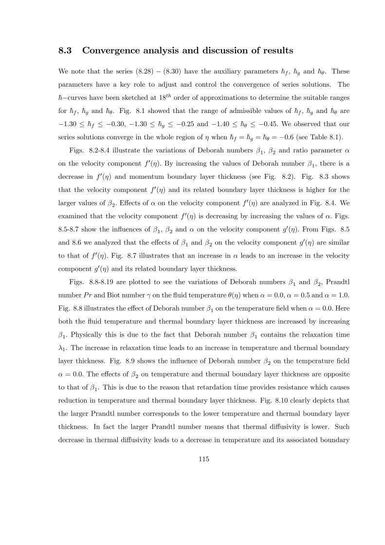
8.3 Convergence analysis and discussion of results
We note that the series (828) − (830) have the auxiliary parameters ~ ~ and ~. Theseparameters have a key role to adjust and control the convergence of series solutions. The
~−curves have been sketched at 18 order of approximations to determine the suitable rangesfor ~ ~ and ~. Fig. 81 showed that the range of admissible values of ~ ~ and ~ are
−130 ≤ ~ ≤ −030 −130 ≤ ~ ≤ −025 and −140 ≤ ~ ≤ −045 We observed that ourseries solutions converge in the whole region of when ~ = ~ = ~ = −06 (see Table 8.1).
Figs. 8.2-8.4 illustrate the variations of Deborah numbers 1 2 and ratio parameter
on the velocity component 0() By increasing the values of Deborah number 1, there is a
decrease in 0() and momentum boundary layer thickness (see Fig. 8.2). Fig. 8.3 shows
that the velocity component 0() and its related boundary layer thickness is higher for the
larger values of 2 Effects of on the velocity component 0() are analyzed in Fig. 8.4. We
examined that the velocity component 0() is decreasing by increasing the values of Figs.
8.5-8.7 show the influences of 1 2 and on the velocity component 0() From Figs. 8.5
and 8.6 we analyzed that the effects of 1 and 2 on the velocity component 0() are similar
to that of 0() Fig. 8.7 illustrates that an increase in leads to an increase in the velocity
component 0() and its related boundary layer thickness.
Figs. 8.8-8.19 are plotted to see the variations of Deborah numbers 1 and 2 Prandtl
number and Biot number on the fluid temperature () when = 00 = 05 and = 10
Fig. 8.8 illustrates the effect of Deborah number 1 on the temperature field when = 00 Here
both the fluid temperature and thermal boundary layer thickness are increased by increasing
1 Physically this is due to the fact that Deborah number 1 contains the relaxation time
1. The increase in relaxation time leads to an increase in temperature and thermal boundary
layer thickness. Fig. 8.9 shows the influence of Deborah number 2 on the temperature field
= 00 The effects of 2 on temperature and thermal boundary layer thickness are opposite
to that of 1. This is due to the reason that retardation time provides resistance which causes
reduction in temperature and thermal boundary layer thickness. Fig. 8.10 clearly depicts that
the larger Prandtl number corresponds to the lower temperature and thermal boundary layer
thickness. In fact the larger Prandtl number means that thermal diffusivity is lower. Such
decrease in thermal diffusivity leads to a decrease in temperature and its associated boundary
115
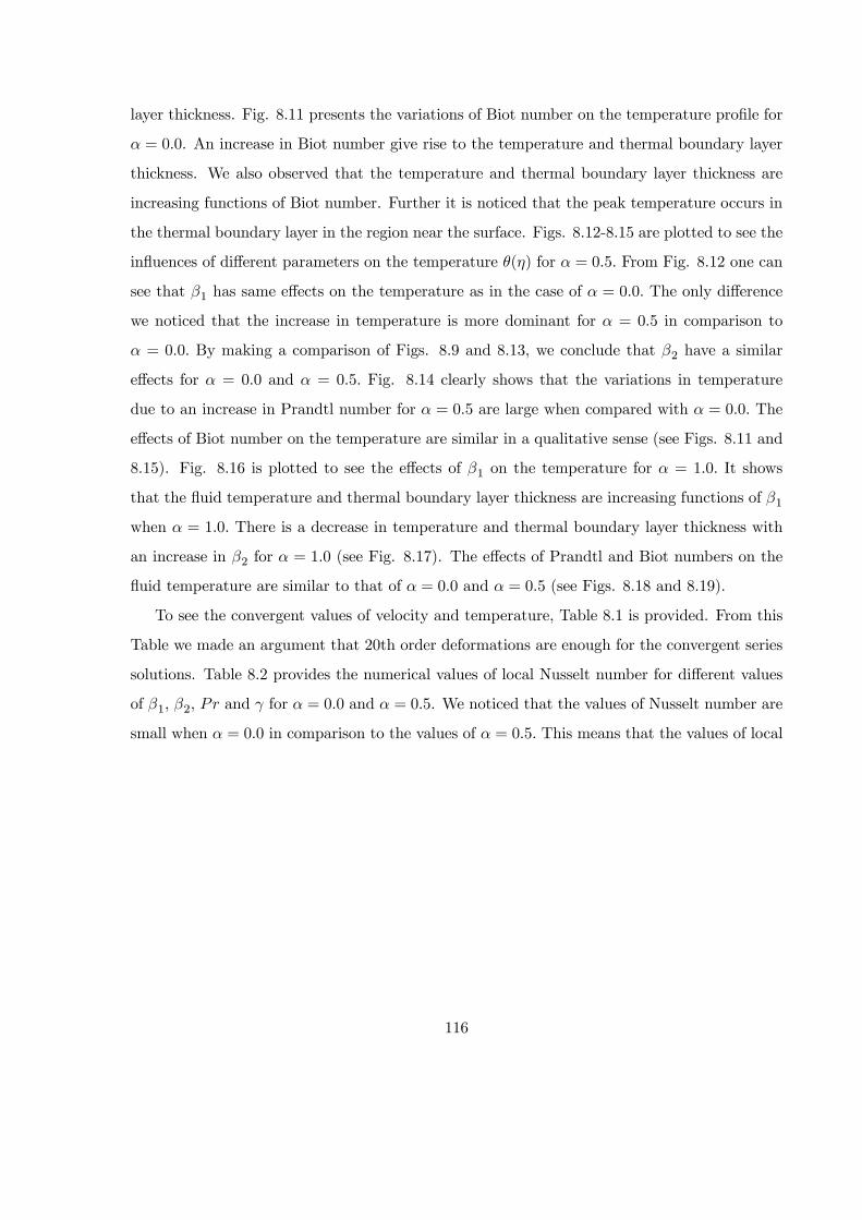
layer thickness. Fig. 8.11 presents the variations of Biot number on the temperature profile for
= 00. An increase in Biot number give rise to the temperature and thermal boundary layer
thickness. We also observed that the temperature and thermal boundary layer thickness are
increasing functions of Biot number. Further it is noticed that the peak temperature occurs in
the thermal boundary layer in the region near the surface. Figs. 8.12-8.15 are plotted to see the
influences of different parameters on the temperature () for = 05 From Fig. 8.12 one can
see that 1 has same effects on the temperature as in the case of = 00 The only difference
we noticed that the increase in temperature is more dominant for = 05 in comparison to
= 00 By making a comparison of Figs. 8.9 and 8.13, we conclude that 2 have a similar
effects for = 00 and = 05 Fig. 8.14 clearly shows that the variations in temperature
due to an increase in Prandtl number for = 05 are large when compared with = 00 The
effects of Biot number on the temperature are similar in a qualitative sense (see Figs. 8.11 and
8.15). Fig. 8.16 is plotted to see the effects of 1 on the temperature for = 10 It shows
that the fluid temperature and thermal boundary layer thickness are increasing functions of 1
when = 10 There is a decrease in temperature and thermal boundary layer thickness with
an increase in 2 for = 10 (see Fig. 8.17). The effects of Prandtl and Biot numbers on the
fluid temperature are similar to that of = 00 and = 05 (see Figs. 8.18 and 8.19).
To see the convergent values of velocity and temperature, Table 8.1 is provided. From this
Table we made an argument that 20th order deformations are enough for the convergent series
solutions. Table 8.2 provides the numerical values of local Nusselt number for different values
of 1 2 and for = 00 and = 05. We noticed that the values of Nusselt number are
small when = 00 in comparison to the values of = 05 This means that the values of local
116
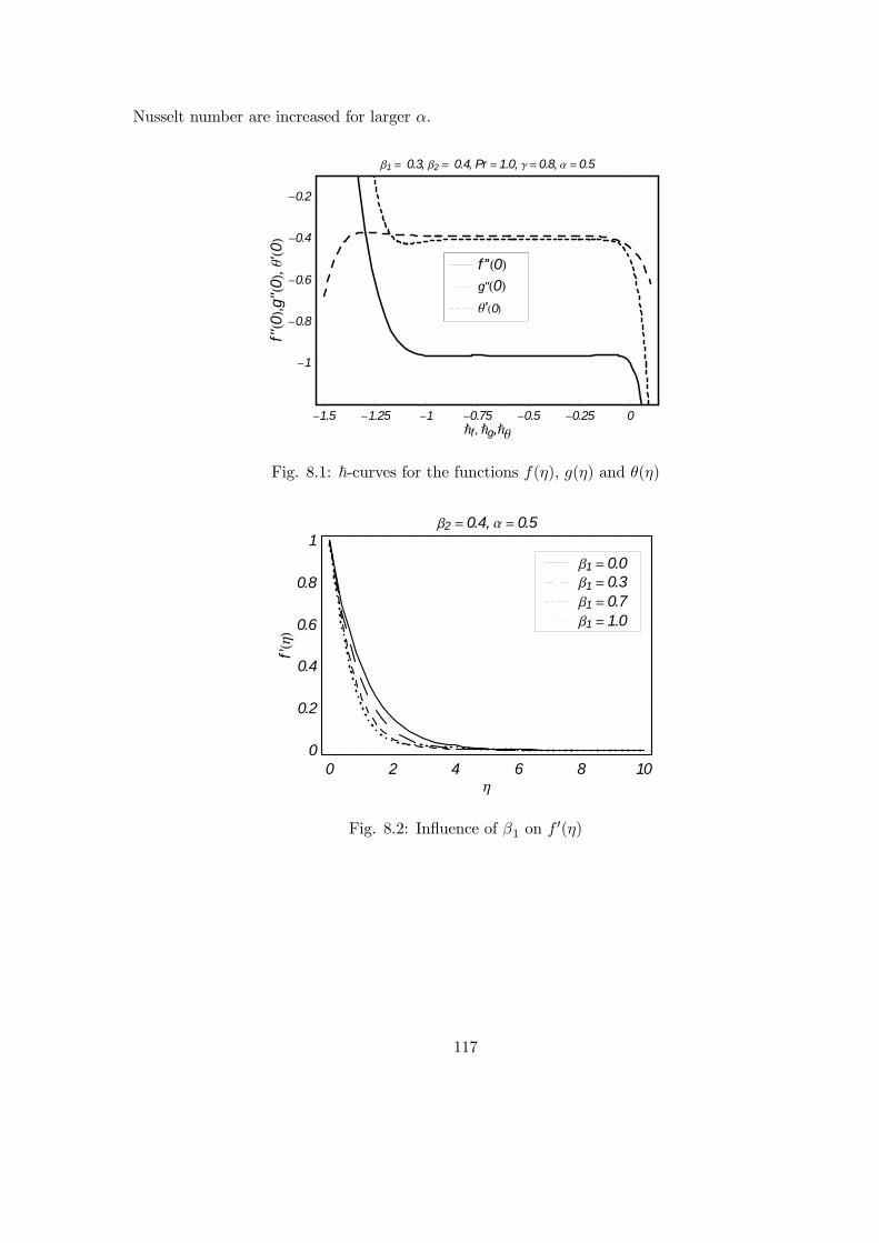
Nusselt number are increased for larger
-1.5 -1.25 -1 -0.75 -0.5 -0.25 0Ñf ,Ñg,Ñq
-1
-0.8
-0.6
-0.4
-0.2
f''0
,g''0
,q'0
b1 = 0.3, b2 = 0.4, Pr = 1.0, g = 0.8, a = 0.5
q'0g''0f ''0
Fig. 8.1: ~-curves for the functions () () and ()
0 2 4 6 8 10h
0
0.2
0.4
0.6
0.8
1
f'h
b2 = 0.4, a = 0.5
b1 = 1.0b1 = 0.7b1 = 0.3b1 = 0.0
Fig. 8.2: Influence of 1 on 0()
117

0 2 4 6 8 10h
0
0.2
0.4
0.6
0.8
1
f'h
b1 = 0.4, a = 0.5
b2 = 1.0b2 = 0.7b2 = 0.3b2 = 0.0
Fig. 8.3: Influence of 2 on 0()
0 2 4 6 8 10h
0
0.2
0.4
0.6
0.8
1
f'h
b1 = 0.4= b2
a = 1.0a = 0.7a = 0.4a = 0.0
Fig. 8.4: Influence of on 0()
118
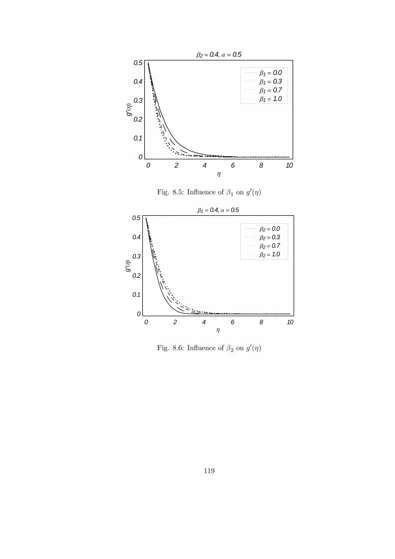
0 2 4 6 8 10h
0
0.1
0.2
0.3
0.4
0.5
g'h
b2 = 0.4, a = 0.5
b1 = 1.0b1 = 0.7b1 = 0.3b1 = 0.0
Fig. 8.5: Influence of 1 on 0()
0 2 4 6 8 10h
0
0.1
0.2
0.3
0.4
0.5
g'h
b1 = 0.4, a = 0.5
b2 = 1.0b2 = 0.7b2 = 0.3b2 = 0.0
Fig. 8.6: Influence of 2 on 0()
119
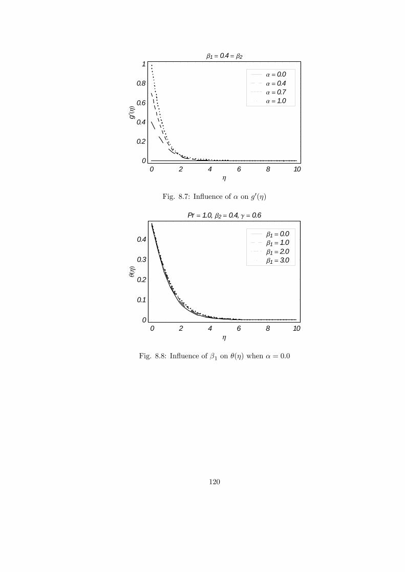
0 2 4 6 8 10h
0
0.2
0.4
0.6
0.8
1
g'h
b1 = 0.4= b2
a = 1.0a = 0.7a = 0.4a = 0.0
Fig. 8.7: Influence of on 0()
0 2 4 6 8 10h
0
0.1
0.2
0.3
0.4
qh
Pr = 1.0, b2 = 0.4, g = 0.6
b1 = 3.0b1 = 2.0b1 = 1.0b1 = 0.0
Fig. 8.8: Influence of 1 on () when = 00
120

0 2 4 6 8 10h
0
0.1
0.2
0.3
0.4
qh
Pr = 1.0, b1 = 0.4, g = 0.6
b2 = 3.0b2 = 2.0b2 = 1.0b2 = 0.0
Fig. 8.9: Influence of 2 on () when = 00
0 2 4 6 8 10h
0
0.1
0.2
0.3
0.4
0.5
qh
b1 = b2 = 0.4, g = 0.6
Pr = 1.5Pr = 1.0Pr = 0.5Pr = 0.1
Fig. 8.10: Influence of Pr on () when = 00
121
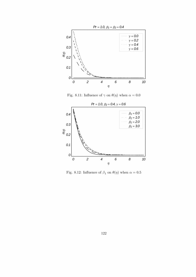
0 2 4 6 8 10h
0
0.1
0.2
0.3
0.4
qh
Pr = 1.0, b1 = b2 = 0.4
g = 0.6g = 0.4g = 0.2g = 0.0
Fig. 8.11: Influence of on () when = 00
0 2 4 6 8 10h
0
0.1
0.2
0.3
0.4
qh
Pr = 1.0, b2 = 0.4, g = 0.6
b1 = 3.0b1 = 2.0b1 = 1.0b1 = 0.0
Fig. 8.12: Influence of 1 on () when = 05
122
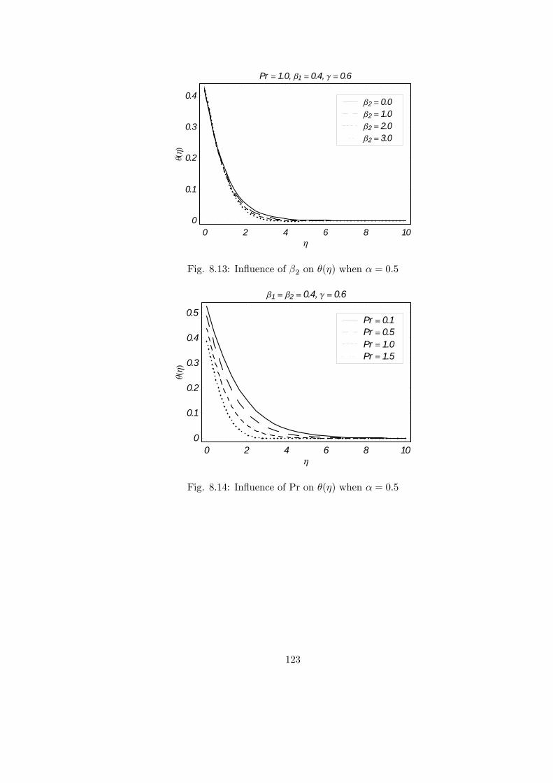
0 2 4 6 8 10h
0
0.1
0.2
0.3
0.4
qh
Pr = 1.0, b1 = 0.4, g = 0.6
b2 = 3.0b2 = 2.0b2 = 1.0b2 = 0.0
Fig. 8.13: Influence of 2 on () when = 05
0 2 4 6 8 10h
0
0.1
0.2
0.3
0.4
0.5
qh
b1 = b2 = 0.4, g = 0.6
Pr = 1.5Pr = 1.0Pr = 0.5Pr = 0.1
Fig. 8.14: Influence of Pr on () when = 05
123

0 2 4 6 8 10h
0
0.1
0.2
0.3
0.4
qh
Pr = 1.0, b1 = b2 = 0.4
g = 0.6g = 0.4g = 0.2g = 0.0
Fig. 8.15: Influence of on () when = 05
0 2 4 6 8 10h
0
0.1
0.2
0.3
0.4
qh
Pr = 1.0, b2 = 0.4, g = 0.6
b1 = 3.0b1 = 2.0b1 = 1.0b1 = 0.0
Fig. 8.16: Influence of 1 on () when = 10
124
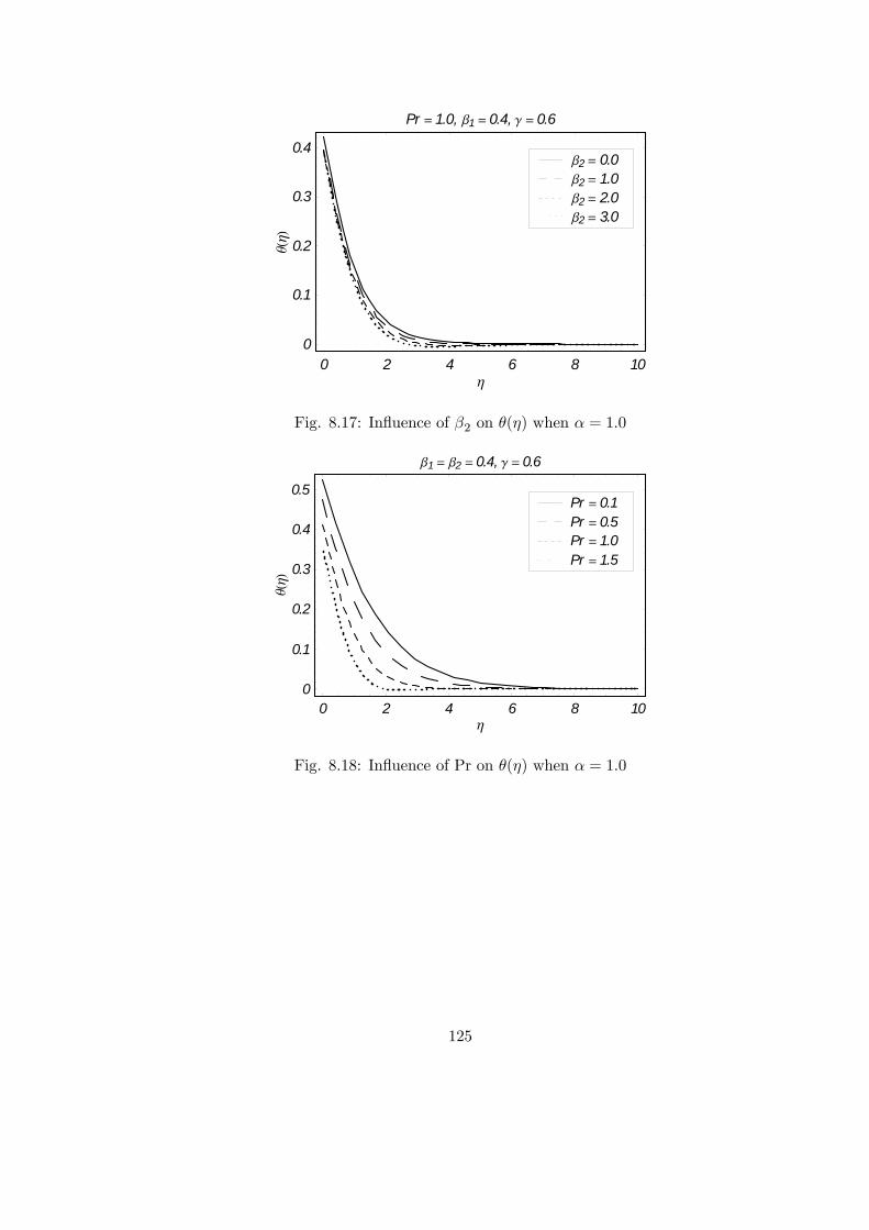
0 2 4 6 8 10h
0
0.1
0.2
0.3
0.4
qh
Pr = 1.0, b1 = 0.4, g = 0.6
b2 = 3.0b2 = 2.0b2 = 1.0b2 = 0.0
Fig. 8.17: Influence of 2 on () when = 10
0 2 4 6 8 10h
0
0.1
0.2
0.3
0.4
0.5
qh
b1 = b2 = 0.4, g = 0.6
Pr = 1.5Pr = 1.0Pr = 0.5Pr = 0.1
Fig. 8.18: Influence of Pr on () when = 10
125
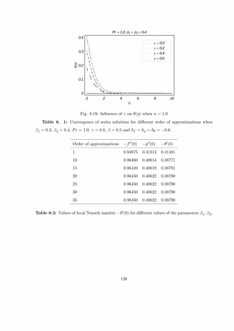
0 2 4 6 8 10h
0
0.1
0.2
0.3
0.4
qh
Pr = 1.0, b1 = b2 = 0.4
g = 0.6g = 0.4g = 0.2g = 0.0
Fig. 8.19: Influence of on () when = 10
Table 8. 1: Convergence of series solutions for different order of approximations when
1 = 03 2 = 04 = 10 = 08 = 05 and ~ = ~ = ~ = −06
Order of approximations − 00(0) −00(0) −0(0)1 0.94875 0.41313 0.41481
10 0.96460 0.40614 0.38771
15 0.96449 0.40619 0.38791
20 0.96450 0.40622 0.38790
25 0.96450 0.40622 0.38790
30 0.96450 0.40622 0.38790
35 0.96450 0.40622 0.38790
Table 8.2: Values of local Nusselt number −0(0) for different values of the parameters 1 2
126
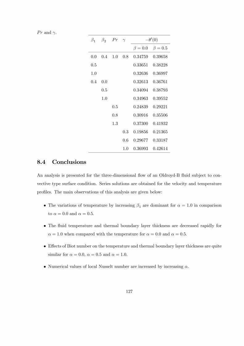
and .
1 2 −0(0) = 00 = 05
0.0 0.4 1.0 0.8 0.34759 0.39658
0.5 0.33651 0.38228
1.0 0.32636 0.36997
0.4 0.0 0.32613 0.36761
0.5 0.34094 0.38793
1.0 0.34963 0.39552
0.5 0.24839 0.29221
0.8 0.30916 0.35506
1.3 0.37300 0.41932
0.3 0.19856 0.21365
0.6 0.29677 0.33187
1.0 0.36993 0.42614
8.4 Conclusions
An analysis is presented for the three-dimensional flow of an Oldroyd-B fluid subject to con-
vective type surface condition. Series solutions are obtained for the velocity and temperature
profiles. The main observations of this analysis are given below:
• The variations of temperature by increasing 1 are dominant for = 10 in comparisonto = 00 and = 05
• The fluid temperature and thermal boundary layer thickness are decreased rapidly for = 10 when compared with the temperature for = 00 and = 05
• Effects of Biot number on the temperature and thermal boundary layer thickness are quitesimilar for = 00 = 05 and = 10
• Numerical values of local Nusselt number are increased by increasing
127

• Values of local Nusselt number are smaller for = 00 when compared with = 05 (see
Table 8.2).
128
Chapter 9
Radiative flow of Jeffrey fluid in a
porous medium with power law heat
flux and heat source
The aim of this chapter is to examine the flow of an incompressible Jeffrey fluid over a stretching
surface. In addition the heat transfer process subject to power law heat flux and heat source
is addressed. Mathematical analysis has been carried out in the presence of thermal radiation.
Homotopic solutions for the velocity and temperature are developed. The related convergence
analysis is made very carefully. The plotted results are discussed for the temperature and heat
transfer characteristics.
9.1 Governing problems
We consider the two-dimensional flow of an incompressible Jeffrey fluid over a moving porous
surface in the presence of power law heat flux and heat source. Thermal radiation effects are
also accounted. A Cartesian coordinate system is chosen in such a way that −axis is alongthe stretching surface and the −axis perpendicular to it. The fluid fills the porous half space 0. The boundary layer equations for flow and temperature are given by
+
= 0 (9.1)
129
+
=
1 + ∗
∙2
2+ 2
µ
3
2−
2
2+
2
+
3
3
¶¸−
(9.2)
+
=
2
2−
( − ∞)−
(9.3)
where and are the velocity components in the − and −directions, ∗ and 2 are the ratioof relaxation to retardation times and retardation time respectively, = () is the kinematic
viscosity, is the permeability of porous medium, is the fluid temperature, is the density of
fluid, is the thermal conductivity of fluid, is the specific heat at constant pressure, is the
heat source coefficient and is the radiative heat flux. By using the Rosseland approximation
we have
= −4∗
31
4
(9.4)
where ∗ is the Stefan-Boltzmann constant and 1 is the mean absorption coefficient. Taylor’s
series helps in writing the following expressions
4 ∼= 4 3∞ − 3 4∞ (9.5)
One can write now after employing the Eqs. (93)− (95) as follows
+
=
2
2−
( − ∞) +
16 3∞3∗
2
2 (9.6)
The boundary conditions are defined by
= = −0
= 2 at = 0 (9.7)
= 0 = ∞ as →∞ (9.8)
where is the temperature coefficient and ∞ is the ambient temperature.
We introduce the similarity transformations
= 0() = −√() = ∞ +
r
2() =
r
(9.9)
130
Here is a constant and prime denotes differentiation with respect to .
Using Eq. (98) we have
000 + ( 002 − 0000) + (1 + ∗)( 00 − 02)− 1(1 + ∗) 0 = 0 (9.10)
(1 +4
3)00 + 0 − 2 0 − ∗ = 0 (9.11)
= ∗ 0 = 1 0 = −1 at = 0 (9.12)
0 = 0 = 0 as →∞ (9.13)
where Eq. (91) is satisfied automatically and = 2 is the Deborah number =
is the
permeability parameter, ∗ = 0√is the suction parameter, =
is the Prandtl number
and ∗ = is a heat generation parameter.
Expression of local Nusselt number with heat transfer is
=
( − ∞) = −
µ
¶=0
(9.14)
Dimensionless form of Eq. (914) gives
12 = − 1
(0) (9.15)
9.2 Homotopy analysis solutions
We can express and by a set of base functions
{ exp(−) ≥ 0 ≥ 0} (9.16)
in the forms
() =
∞X=0
∞X=0
exp(−) (9.17)
() =
∞X=0
∞X=0
exp(−) (9.18)
131

in which and are the coefficients. We further choose the following initial approxima-
tions and auxiliary linear operators
0() = ∗ + 1− exp(−) 0() = − exp(−) (9.19)
L = 000 − 0 L = 00 + 0 (9.20)
with
L (1 + 2 + 3
−) = 0 L(4 + 5−) = 0 (9.21)
where ( = 1− 5) represent the arbitrary constants.The zeroth order deformation problems are
(1− )Lh(; )− 0()
i= ~N
h(; )
i (9.22)
(1− )Lh(; )− 0()
i= ~N
h(; ) ( )
i (9.23)
(0; ) = ∗ 0(0; ) = 1 0(∞; ) = 0 0(0 ) = 1 (∞ ) = 0 (9.24)
N [( )] =3( )
3+ (1 + ∗)( )
2( )
2− (1 + ∗)
Ã( )
!2
+2
"2( )
( )
2( )
2− (( ))2
3( )
3
#− 1
(1 + )
( )
(9.25)
N[( ) ( )] =
µ1 +
4
3
¶2( )
2+( )
( )
−2( )
( )−∗( )
(9.26)
in which is an embedding parameter, ~ and ~ the non zero auxiliary parameters and N
and N the nonlinear operators.
For = 0 and = 1 we have
(; 0) = 0() ( 0) = 0() and (; 1) = () ( 1) = () (9.27)
and when increases from 0 to 1 then ( ) and ( ) vary from 0() 0() to () and
132

() By Taylor’s’ series one has
( ) = 0() +∞P
=1
() (9.28)
( ) = 0() +∞P
=1
() (9.29)
() =1
!
(; )
¯=0
() =1
!
(; )
¯=0
(9.30)
where the convergence of above series strongly depends upon ~ and ~ Considering that ~
and ~ are selected properly so that Eqs. (922) and (923) converge at = 1 and thus we have
() = 0() +∞P
=1
() (9.31)
() = 0() +∞P
=1
() (9.32)
The problems at th-order are
L [()− −1()] = ~R () (9.33)
L[()− −1()] = ~R () (9.34)
(0) = 0(0) = 0(∞) = 0 0(0) = (∞) = 0 (9.35)
R () = 000−1() + (1 + ∗)
−1P=0
h−1− 00 − 0−1−
000
i+2
−1X=0
−1−X=0
{2 0− 00 − − 000 − (1 + ∗)1
0−1() (9.36)
R () = 00−1 +
−1P=0
0−1− − 2−1P=0
−1− 0 − ∗ (9.37)
=
⎡⎣ 0 ≤ 11 1
(9.38)
133

The general solutions can be expressed in the forms
() = ∗() + 1 + 2 +3
− (9.39)
() = ∗() + 4 + 5− (9.40)
in which ∗ and ∗ indicate the special solutions.
9.3 Convergence of the homotopy solutions
As we know that the auxiliary parameters ~ and ~ play indispensable role to adjust and
control the convergence of the homotopy solutions. For the range of admissible values of ~
and ~ we plot the ~−curves for 16-order of approximations. Figs. 91 and 92 show thatthe range of admissible values of ~ and ~ are −13 ≤ ~ ≤ −025 and −085 ≤ ~ ≤ −025Further the series converges in the whole region of when ~ = −10 and ~ = −06 FromTable 91 we see that our series solutions converge from 20 order of approximations Hence
25 order approximations are enough for the convergent solutions.
-1.2 -1 -0.8 -0.6 -0.4 -0.2 0Ñf
-1.7
-1.6
-1.5
-1.4
-1.3
-1.2
-1.1
-1
f''0
N=0.4, S* = 0.5, Pr =1.0, l = 1.0, b2 =0.1, b* = 0.2, l* =0.2
f''0
Fig. 9.1: ~−curve for the function ()
134
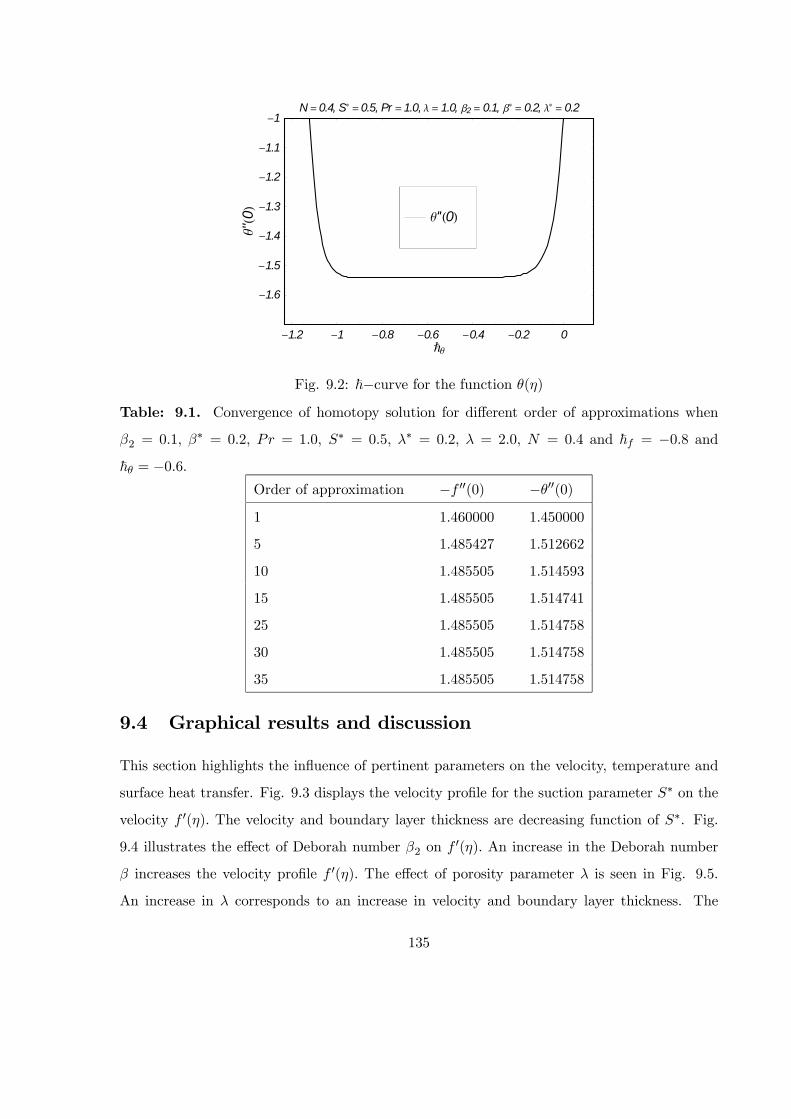
-1.2 -1 -0.8 -0.6 -0.4 -0.2 0Ñq
-1.6
-1.5
-1.4
-1.3
-1.2
-1.1
-1
q''0
N=0.4, S* =0.5, Pr =1.0, l = 1.0, b2 = 0.1, b* = 0.2, l* = 0.2
q''0
Fig. 9.2: ~−curve for the function ()
Table: 9.1. Convergence of homotopy solution for different order of approximations when
2 = 01 ∗ = 02 = 10, ∗ = 05 ∗ = 02 = 20 = 04 and ~ = −08 and~ = −06
Order of approximation − 00(0) −00(0)1 1.460000 1.450000
5 1.485427 1.512662
10 1.485505 1.514593
15 1.485505 1.514741
25 1.485505 1.514758
30 1.485505 1.514758
35 1.485505 1.514758
9.4 Graphical results and discussion
This section highlights the influence of pertinent parameters on the velocity, temperature and
surface heat transfer. Fig. 93 displays the velocity profile for the suction parameter ∗ on the
velocity 0() The velocity and boundary layer thickness are decreasing function of ∗. Fig.
9.4 illustrates the effect of Deborah number 2 on 0() An increase in the Deborah number
increases the velocity profile 0() The effect of porosity parameter is seen in Fig. 9.5.
An increase in corresponds to an increase in velocity and boundary layer thickness. The
135
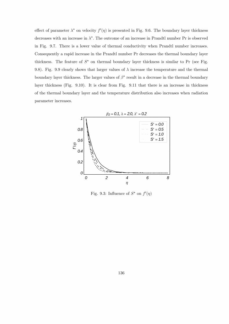
effect of parameter ∗ on velocity 0() is presented in Fig. 9.6. The boundary layer thickness
decreases with an increase in ∗ The outcome of an increase in Prandtl number Pr is observed
in Fig. 9.7. There is a lower value of thermal conductivity when Prandtl number increases.
Consequently a rapid increase in the Prandtl number Pr decreases the thermal boundary layer
thickness. The feature of ∗ on thermal boundary layer thickness is similar to Pr (see Fig.
9.8). Fig. 99 clearly shows that larger values of increase the temperature and the thermal
boundary layer thickness. The larger values of ∗ result in a decrease in the thermal boundary
layer thickness (Fig. 9.10). It is clear from Fig. 9.11 that there is an increase in thickness
of the thermal boundary layer and the temperature distribution also increases when radiation
parameter increases.
0 2 4 6 8h
0
0.2
0.4
0.6
0.8
1
f'h
b2 = 0.1, l = 2.0, l* = 0.2
S* = 1.5S* = 1.0S* = 0.5S* = 0.0
Fig. 9.3: Influence of ∗ on 0()
136

0 2 4 6 8h
0
0.2
0.4
0.6
0.8
1
f'h
S* = 0.5, l = 2.0, l* = 0.2
b2 = 1.0b2 = 0.6b2 = 0.3b2 = 0.0
Fig. 9.4: Influence of 2 on 0()
0 2 4 6 8h
0
0.2
0.4
0.6
0.8
1
f'h
S* = 0.5, b2 = 0.1, l* = 0.2
l = 3.0l = 2.0l = 1.0l = 0.5
Fig. 9.5: Influence of on 0()
137
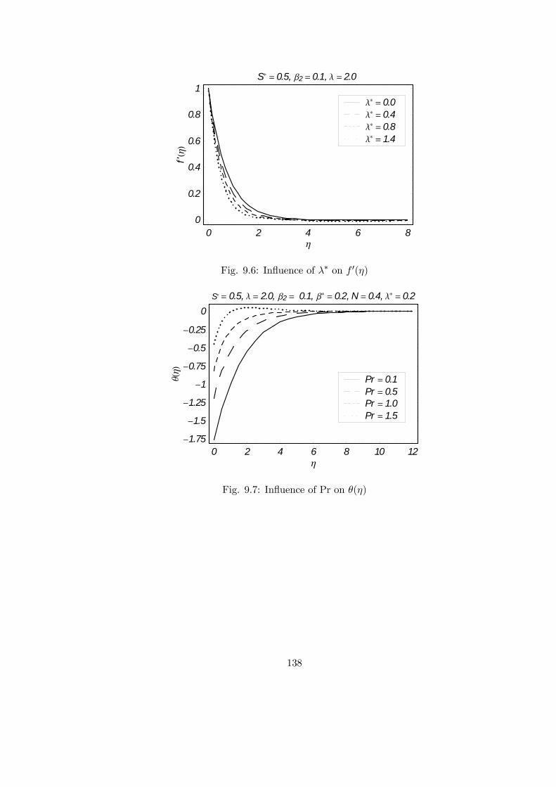
0 2 4 6 8h
0
0.2
0.4
0.6
0.8
1
f'h
S* = 0.5, b2 = 0.1, l = 2.0
l* = 1.4l* = 0.8l* = 0.4l* = 0.0
Fig. 9.6: Influence of ∗ on 0()
0 2 4 6 8 10 12h
-1.75
-1.5
-1.25
-1
-0.75
-0.5
-0.25
0
qh
S* = 0.5, l = 2.0, b2 = 0.1, b* = 0.2, N = 0.4, l* = 0.2
Pr = 1.5Pr = 1.0Pr = 0.5Pr = 0.1
Fig. 9.7: Influence of Pr on ()
138
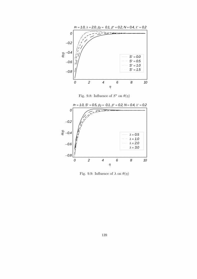
0 2 4 6 8 10h
-0.8
-0.6
-0.4
-0.2
0
qh
Pr = 1.0, l = 2.0, b2 = 0.1, b* = 0.2, N = 0.4, l* = 0.2
S* = 1.5S* = 1.0S* = 0.5S* = 0.0
Fig. 9.8: Influence of ∗ on ()
0 2 4 6 8 10h
-0.8
-0.6
-0.4
-0.2
0
qh
Pr = 1.0, S* = 0.5, b2 = 0.1, b* = 0.2, N= 0.4, l* = 0.2
l = 3.0l = 2.0l = 1.0l = 0.5
Fig. 9.9: Influence of on ()
139
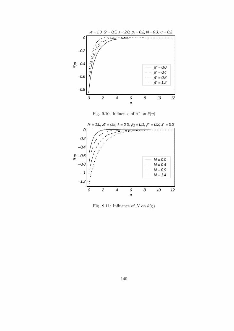
0 2 4 6 8 10 12h
-0.8
-0.6
-0.4
-0.2
0
qh
Pr = 1.0, S* = 0.5, l = 2.0, b2 = 0.2, N = 0.3, l* = 0.2
b* = 1.2b* = 0.8b* = 0.4b* = 0.0
Fig. 9.10: Influence of ∗ on ()
0 2 4 6 8 10 12h
-1.2
-1
-0.8
-0.6
-0.4
-0.2
0
qh
Pr = 1.0, S* = 0.5, l = 2.0, b2 = 0.1, b* = 0.2, l* = 0.2
N= 1.4N= 0.9N= 0.4N= 0.0
Fig. 9.11: Influence of on ()
140

Table 9.2: Values of local Nusselt number 12 for the different values of parameters
∗ 2 ∗ and when ∗ = 05 and = 04
∗ 2 ∗ −12
0.5 0.2 0.1 0.2 1.0 1.13518
1.0 1.17909
2.0 1.20704
2.0 0.0 1.22933
0.4 1.18641
0.8 1.14936
0.0 1.17970
0.3 1.24496
0.6 1.28144
0.0 1.11523
0.5 1.31994
1.0 1.47567
0.4 0.71664
0.8 1.05025
1.5 1.57240
9.5 Final remarks
Steady flow of Jeffrey fluid in a porous medium is discussed. Analysis has been carried out in
presence of power law heat flux, heat source and thermal radiation. Important points can be
summed up as follows:
• Suction parameter ∗ and Deborah number 2 have similar effects on the velocity profile 0()
• Velocity field 0() increases when the porosity parameter increases
• The temperature profile () increases in view of an increase in Pr
• The heat generation parameter ∗ leads to a decrease in ()
141
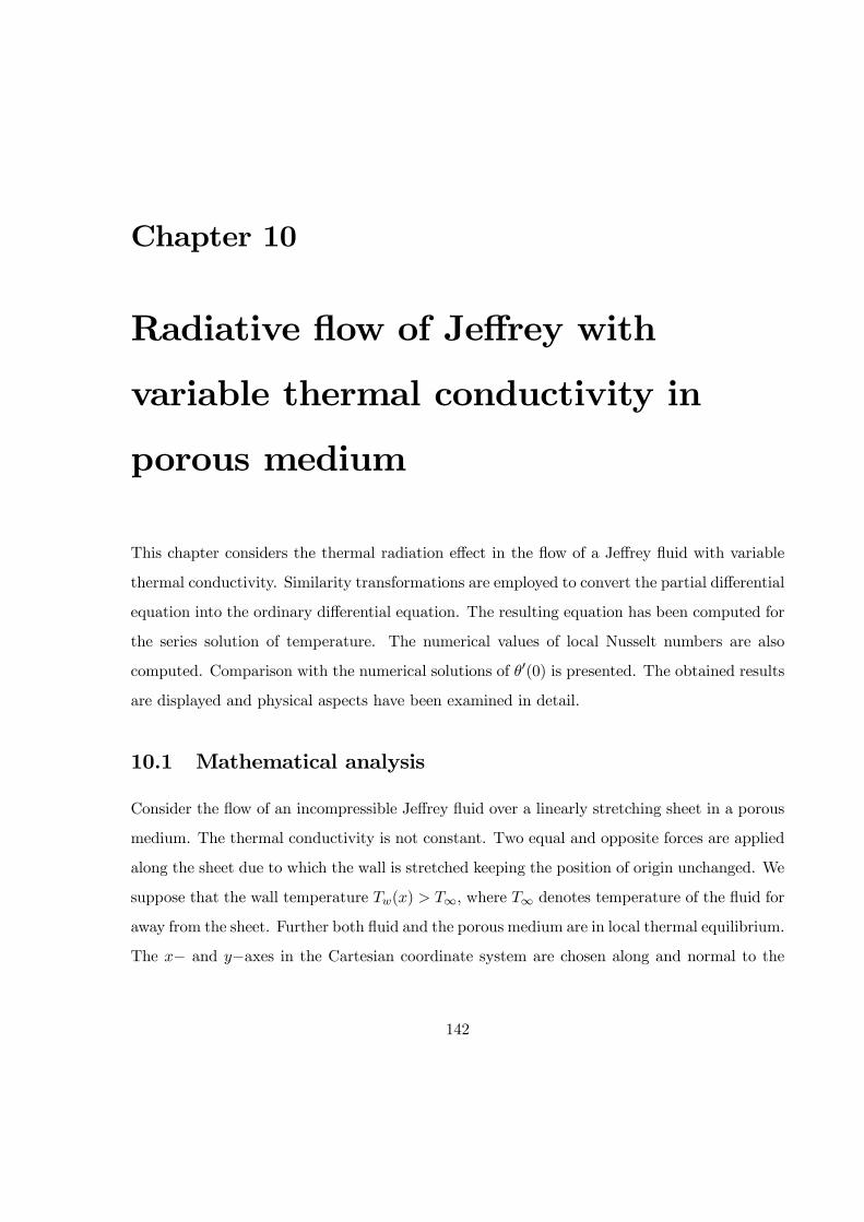
Chapter 10
Radiative flow of Jeffrey with
variable thermal conductivity in
porous medium
This chapter considers the thermal radiation effect in the flow of a Jeffrey fluid with variable
thermal conductivity. Similarity transformations are employed to convert the partial differential
equation into the ordinary differential equation. The resulting equation has been computed for
the series solution of temperature. The numerical values of local Nusselt numbers are also
computed. Comparison with the numerical solutions of 0(0) is presented. The obtained results
are displayed and physical aspects have been examined in detail.
10.1 Mathematical analysis
Consider the flow of an incompressible Jeffrey fluid over a linearly stretching sheet in a porous
medium. The thermal conductivity is not constant. Two equal and opposite forces are applied
along the sheet due to which the wall is stretched keeping the position of origin unchanged. We
suppose that the wall temperature () ∞ where ∞ denotes temperature of the fluid for
away from the sheet. Further both fluid and the porous medium are in local thermal equilibrium.
The − and −axes in the Cartesian coordinate system are chosen along and normal to the
142
sheet respectively. The energy equation subject to radiative effect can be expressed in the form
∙
+
¸=
∙
¸−
(10.1)
and the subjected boundary conditions are
= () = ∞ +∗at = 0 (10.2)
→ ∞ as →∞ (10.3)
where , are the flow velocities in the − and −directions respectively, ∗ the ratio ofrelaxation to retardation times, 2 the retardation time, the kinematic viscosity, the
permeability, the temperature, the variable thermal conductivity, the density of the fluid,
the specific heat at constant pressure and the radiative heat flux. By making use of
Rosseland approximation, the radiative heat flux is given by
= −4∗
31
4
(10.4)
where ∗ is the Stefan-Boltzmann constant and 1 is the mean absorption coefficient. In view
of Taylor’s series, the term 4 can be written as
4 ∼= 4 3∞ − 3 4∞ (10.5)
By making use of Eqs. (104) and (105) Eq. (101) becomes
∙
+
¸=
∙
¸+16 3∞31
2
2 (10.6)
The similarity transformations are defined as follows
= 0() = −√() =
r
() =
− ∞ − ∞
(10.7)
where is the variable wall temperature and () is the non-dimensional form of the temper-
ature. We consider = () = ∞+() at = 0 The variable thermal conductivity is
143
= ∞[1 + ] (here and are positive constants, ∞ is the fluid free stream conductivity)
and is given by
= − ∞
∞ (10.8)
where is a constant, is the thermal conductivity at the wall and prime denotes the differ-
entiation with respect to .
Eqs. (101)− (106) reduce to the following expressions
(1 + )00 + 02 +4
300 = [∗ 0 − 0] (10.9)
(0) = 1 and (∞) = 0 (10.10)
where =
∞ is the Prandtl number and =4 3∞∞ is the radiation parameter. The local
Nusselt number is defined as follows
=
( − ∞) (10.11)
with heat transfer given by
= −µ
¶=0
(10.12)
Dimensionless expression of Eq. (1011) is
12 = −0(0) (10.13)
The problems consisting of Eqs. (109) and (1010) can be computed by a homotopy analysis
method (HAM). For that we express in the set of base function
{ exp(−) ≥ 0 ≥ 0} (10.14)
by
() =
∞X=0
∞X=0
exp(−) (10.15)
with and as the coefficients. The initial approximations and auxiliary linear operators
144
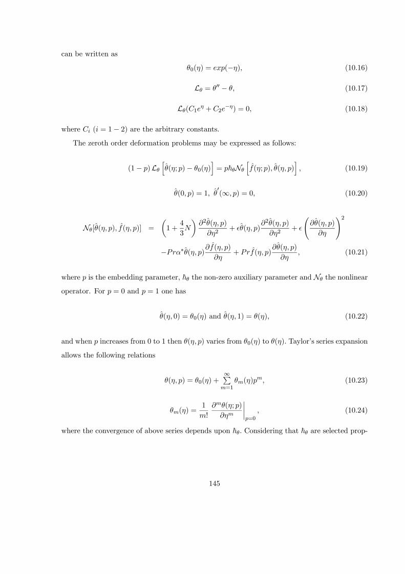
can be written as
0() = (−) (10.16)
L = 00 − (10.17)
L(1 + 2−) = 0 (10.18)
where ( = 1− 2) are the arbitrary constants.The zeroth order deformation problems may be expressed as follows:
(1− )Lh(; )− 0()
i= ~N
h(; ) ( )
i (10.19)
(0 ) = 1 0(∞ ) = 0 (10.20)
N[( ) ( )] =
µ1 +
4
3
¶2( )
2+ ( )
2( )
2+
Ã( )
!2
−∗( )( )
+ ( )( )
(10.21)
where is the embedding parameter, ~ the non-zero auxiliary parameter and N the nonlinear
operator. For = 0 and = 1 one has
( 0) = 0() and ( 1) = () (10.22)
and when increases from 0 to 1 then ( ) varies from 0() to () Taylor’s series expansion
allows the following relations
( ) = 0() +∞P
=1
() (10.23)
() =1
!
(; )
¯=0
(10.24)
where the convergence of above series depends upon ~ Considering that ~ are selected prop-
145
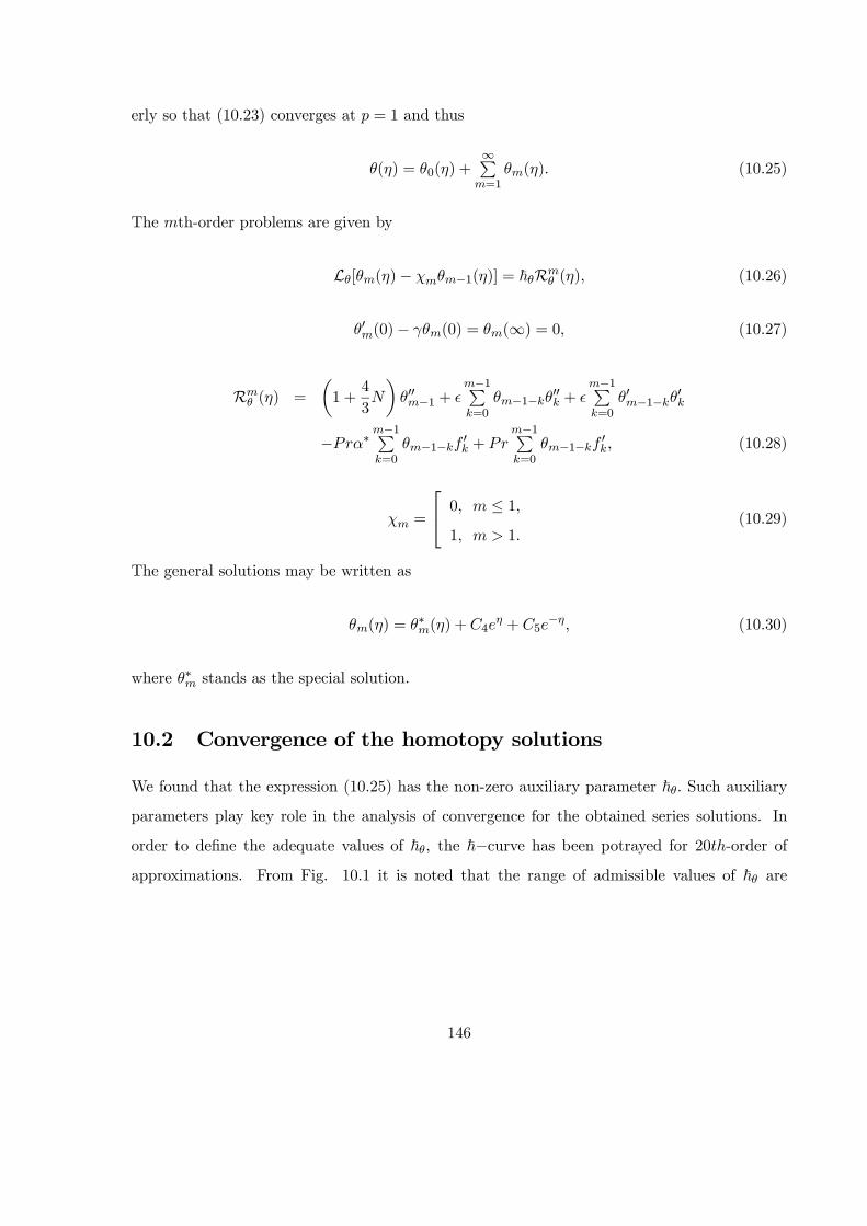
erly so that (1023) converges at = 1 and thus
() = 0() +∞P
=1
() (10.25)
The th-order problems are given by
L[()− −1()] = ~R () (10.26)
0(0)− (0) = (∞) = 0 (10.27)
R () =
µ1 +
4
3
¶00−1 +
−1P=0
−1−00 + −1P=0
0−1−0
−∗−1P=0
−1− 0 + −1P=0
−1− 0 (10.28)
=
⎡⎣ 0 ≤ 11 1
(10.29)
The general solutions may be written as
() = ∗() +4 + 5
− (10.30)
where ∗ stands as the special solution.
10.2 Convergence of the homotopy solutions
We found that the expression (1025) has the non-zero auxiliary parameter ~ Such auxiliary
parameters play key role in the analysis of convergence for the obtained series solutions. In
order to define the adequate values of ~, the ~−curve has been potrayed for 20-order ofapproximations. From Fig. 10.1 it is noted that the range of admissible values of ~ are
146
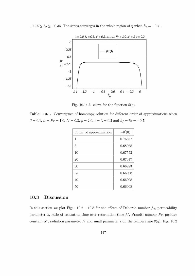
−115 ≤ ~ ≤ −035 The series converges in the whole region of when ~ = −07
-1.4 -1.2 -1 -0.8 -0.6 -0.4 -0.2 0Ñq
-1.5
-1.25
-1
-0.75
-0.5
-0.25
0
q'0
l = 2.0, N=0.3, l* =0.2, b2 = 0.1, Pr = 1.0, a* = 1, e = 0.2
q'0
Fig. 10.1: ~−curve for the function ()
Table: 10.1. Convergence of homotopy solution for different order of approximations when
= 01 = = 10, = 03 = 20 = = 02 and } = } = −07
Order of approximation −0(0)1 0.76667
5 0.68968
10 0.67553
20 0.67017
30 0.66923
35 0.66908
40 0.66908
50 0.66908
10.3 Discussion
In this section we plot Figs. 102 − 108 for the effects of Deborah number 2 permeabilityparameter ratio of relaxation time over retardation time ∗ Prandtl number positive
constant ∗ radiation parameter and small parameter on the temperature (). Fig. 102
147

represents the effects of on () By increasing the temperature () decreases. From Fig.
103 we observed that the temperature field () decreases by increasing the values of ∗ Fig.
104 plots the variations of on () The temperature field () decreases when increases
Fig. 105 shows the effects of 2 on () From Fig. 105 we observed that the temperature field
() decreases when 2 increases. Here Deborah number is directly proportional to retardation
time. An increase in Deborah number implies to the larger retardation time. This larger
retardation time is responsible to a reduction in the temperature and thermal boundary layer
thickness. Fig. 106 shows that the temperature profile () increases when increases. The
larger radiation parameter correspond to higher temperature and smaller radiation parameter
shows lower temperature. An increase in radiation parameter give more to the fluid which
results an enhancement in the temperature and related thermal boundary layer thickness. Fig.
107 plots the effects of on () The temperature field () increases when is increased.
Here is the thermal conductivity parameter. It is a fact that fluid possesses stronger thermal
conductivity has higher temperature. From Figs. 106 and 107 it is obvious that and have
similar effects on the temperature field () in a qualitative sense Fig. 108 shows the effects
of ∗ on temperature profile. We see that () increases by increasing ∗
0 2 4 6 8 10 12h
0
0.2
0.4
0.6
0.8
1
qh
a* = 0.5, l = 2.0, b2 = 0.1, l* = 0.2, N = 0.3, e = 0.2
Pr = 1.5Pr = 1.0Pr = 0.5Pr = 0.1
Fig. 10.2: Influence of Pr on ()
148
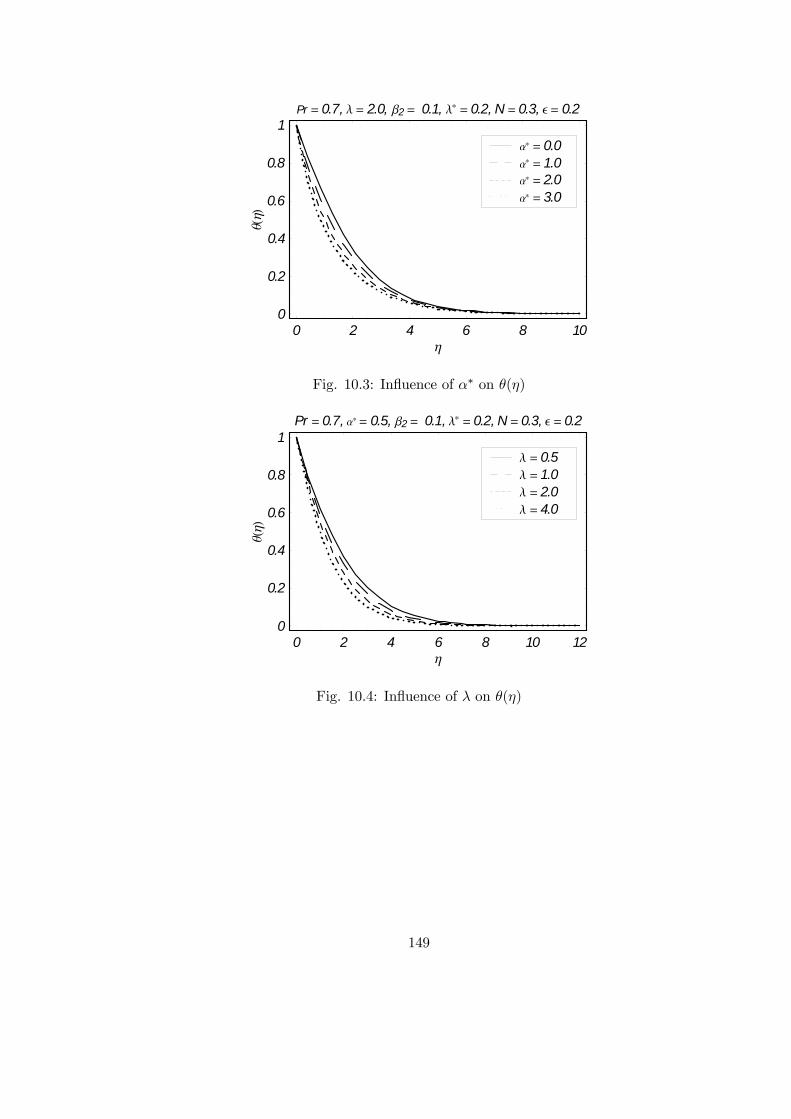
0 2 4 6 8 10h
0
0.2
0.4
0.6
0.8
1
qh
Pr = 0.7, l = 2.0, b2 = 0.1, l* = 0.2, N = 0.3, e = 0.2
a* = 3.0a* = 2.0a* = 1.0a* = 0.0
Fig. 10.3: Influence of ∗ on ()
0 2 4 6 8 10 12h
0
0.2
0.4
0.6
0.8
1
qh
Pr = 0.7, a* = 0.5, b2 = 0.1, l* = 0.2, N = 0.3, e = 0.2
l = 4.0l = 2.0l = 1.0l = 0.5
Fig. 10.4: Influence of on ()
149

0 2 4 6 8 10 12h
0
0.2
0.4
0.6
0.8
1
qh
Pr = 0.7, a* = 0.5, l = 2.0, l* = 0.2, N = 0.3, e = 0.2
b2 = 1.0b2 = 0.6b2 = 0.3b2 = 0.0
Fig. 10.5: Influence of 2 on ()
0 2 4 6 8 10 12h
0
0.2
0.4
0.6
0.8
1
qh
Pr = 0.7, a* = 0.5, l = 2.0, l* = 0.2, b2 = 0.1, e = 0.2
N = 1.2N = 0.8N = 0.4N = 0.0
Fig. 10.6: Influence of on ()
150
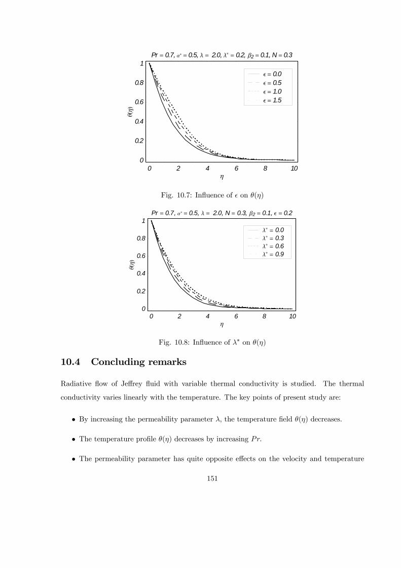
0 2 4 6 8 10h
0
0.2
0.4
0.6
0.8
1
qh
Pr = 0.7, a* = 0.5, l = 2.0, l* = 0.2, b2 = 0.1, N = 0.3
e = 1.5e = 1.0e = 0.5e = 0.0
Fig. 10.7: Influence of on ()
0 2 4 6 8 10h
0
0.2
0.4
0.6
0.8
1
qh
Pr = 0.7, a* = 0.5, l = 2.0, N = 0.3, b2 = 0.1, e = 0.2
l* = 0.9l* = 0.6l* = 0.3l* = 0.0
Fig. 10.8: Influence of ∗ on ()
10.4 Concluding remarks
Radiative flow of Jeffrey fluid with variable thermal conductivity is studied. The thermal
conductivity varies linearly with the temperature. The key points of present study are:
• By increasing the permeability parameter the temperature field () decreases.
• The temperature profile () decreases by increasing
• The permeability parameter has quite opposite effects on the velocity and temperature
151
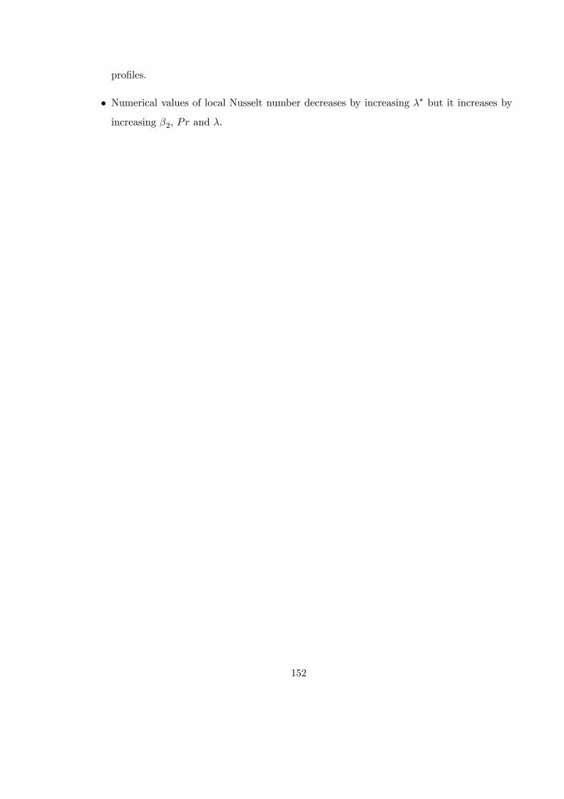
profiles.
• Numerical values of local Nusselt number decreases by increasing ∗ but it increases byincreasing 2 and
152
Chapter 11
Influence of thermophoresis and
Joule heating on the radiative flow of
Jeffrey fluid with mixed convection
This chapter addresses the magnetohydrodynamic (MHD) radiative flow of an incompress-
ible Jeffrey fluid over a linearly stretched surface. Heat and mass transfer characteristics are
accounted in the presence of Joule heating and thermophoretic effects. Series solutions by ho-
motopy analysis method are constructed for the velocity, temperature and concentration fields.
Convergence criteria for the series solutions is established. Numerical values of skin friction
coefficient, local Nusselt and Sherwood numbers are computed and analyzed.
11.1 Flow formulation
We consider Cartesian coordinate system in such a way that −axis is along the stretchingsurface and −axis is perpendicular to the −axis. Magnetohydrodynamic boundary layer flowof Jeffrey fluid is considered. A uniform magnetic field B0 is applied parallel to the −axis.Induced magnetic field is neglected for small magnetic Reynolds number. Heat and mass transfer
characteristics are taken into account in the presence of thermal radiation and thermophoresis
effects. Uniform temperature of the surface is larger than the ambient fluid temperature
∞ The species concentration at the surface and ambient concentration ∞ are constants.
153
Invoking Rosseland approximation, the resulting equations take the following forms
+
= 0 (11.1)
+
=
1 + ∗
µ2
2+ 2
µ
3
2+
3
3−
2
2+
2
¶¶−
∗20
+ [ ( − ∞) + ( −∞)] (11.2)
+
=
2
2+16 3∞3∗
2
2+
µ
¶2+
∗20
2 (11.3)
+
=
2
2−
() (11.4)
Here ( ) are the velocity components along the − and −axes, ∗ and 2 are the ratio
of relaxation/retardation times and retardation time, respectively, the dynamic viscosity,
the density of fluid, ∗ the electrical conductivity, the gravitational acceleration, and
the thermal expansion coefficients, the temperature, the specific heat, the Stefan-
Boltzmann constant, ∗ the mean absorption coefficient, the diffusion coefficient and the
thermophoretic velocity.
The associated boundary conditions are
= = = 0 = () = () at = 0
→ 0
→ 0 → ∞ → ∞ as →∞ (11.5)
where is the stretching velocity, is the temperature at the wall, is the concentration
at the wall and ∞ and ∞ are the ambient fluid temperature and concentration, respectively.
The term in Eq. (11.4) can be defined as follows:
= −1
(11.6)
in which 1 is the thermophoretic coefficient and is the reference temperature. A ther-
154
mophoretic parameter is defined by the following relation
= −1( − ∞)
(11.7)
The wall temperature and concentration fields are
= ∞ + = ∞ + (11.8)
where and are the positive constants.
Through the following transformations
= 0() = −√() =
r
() = − ∞ − ∞
() = − ∞ − ∞
(11.9)
equation (11.1) is automatically satisfied and the Eqs. (11.2)-(11.4) are reduced as follows:
000 + (1+ ∗)( 00 − 02) + 2(002 − 0000)− (1 + ∗)2 0 + (1+ ∗)1(+ 2) = 0 (11.10)
(1 +4
3)00 + [0 − 0] + 002 +2 02 = 0 (11.11)
00 + (0 − 0)− (00 − 00) = 0 (11.12)
= 0 0 = 1 = 1 = 1 at = 0
0 → 0 00 → 0 → 0 → 0 as →∞ (11.13)
In the above expressions, 2 = 2 is the Deborah number 2 = ∗20 the Hartmann
number, 1 =2
the local buoyancy parameter, = (−∞)32
222
the local Grashof
number, 2 =(−∞) (−∞) the constant dimensionless concentration buoyancy parameter, =
the Prandtl number, =
4∗ 3∞∗ the radiation parameter, =
2(−∞) the Eckert
number and = the Schmidt number.
Skin friction coefficient, local Nusselt number and local Sherwood number are transformed
155
to the following
12 =1
1 + ∗( 00(0) + 2
00(0)), −12 = −0(0) and −12 = −0(0) (11.14)
11.2 Series solutions
The homotopic solutions for , and in a set of base functions
{ exp(−) ≥ 0 ≥ 0} (11.15)
can be written to the following expressions
() =
∞X=0
∞X=0
exp(−) (11.16)
() =
∞X=0
∞X=0
exp(−) (11.17)
() =
∞X=0
∞X=0
exp(−) (11.18)
in which , and are the coefficients. Initial guesses and auxiliary linear operators
are
0() = (1− exp(−) 0() = exp(−), 0() = exp(−), (11.19)
L = 000 − 0 L = 00 − L = 00 − (11.20)
The operators in Eq. (11.19) satisfy the following properties
L (1 + 2 + 3
−) = 0, L(4 + 5−) = 0 L(6 + 7
−) (11.21)
where ( = 1 − 7) denote the arbitrary constants. The zeroth order deformation problemsare expressible in the form
(1− )L³(; )− 0()
´= ~N
³(; ) (; ) (; )
´ (11.22)
156
(1− )L³(; )− 0()
´= ~N
³(; ) (; ) (; )
´ (11.23)
(1− )L³(; )− 0()
´= ~N
³(; ) (; ) (; )
´ (11.24)
(0; ) = 0 0(0; ) = 1 0(∞; ) = 0 00(∞; ) = 0
(0; ) = 1, (∞; ) = 0 (0; ) = 1 and (∞; ) = 0 (11.25)
Here shows embedding parameter, ~ , ~ and ~ the non-zero auxiliary parameters and the
nonlinear operators N , N and N are given by
N [( ) (; ) (; )] =3( )
3+ (1 + ∗)
⎛⎝( )2( )
2−Ã( )
!2⎞⎠+2
⎛⎝Ã2( )
2
!2− ( )
4( )
4
⎞⎠− (1 + ∗)2( )
+(1 + ∗)³1(( ) + 2(; )
´ (11.26)
N[( ) (; ) (; )] =
µ1 +
4
3
¶2( )
2+
Ã2( )
2
!2+2
Ã( )
!2
−( )( )
+ ( )( )
(11.27)
N[( ) (; ) (; )] =2( )
2+
Ã( )
( )
− ( )
( )
!
−Ã( )
( )
− ( )
2( )
2
! (11.28)
When = 0 and = 1 one has
(; 0) = 0(); (; 1) = () (11.29)
(; 0) = 0(); (; 1) = () (11.30)
157
(; 0) = 0(); (; 1) = () (11.31)
Note that when increases from 0 to 1 then ( ), ( ) and ( ) approach 0() to (),
0() to () and 0() to () According to Taylor’s series one has
( ) = 0() +∞P
=1
() () =
1
!
(; )
¯=0
(11.32)
( ) = 0() +∞P
=1
() () =
1
!
(; )
¯=0
(11.33)
( ) = 0() +∞P
=1
() () =
1
!
(; )
¯=0
(11.34)
The convergence of series (11.22)-(11.24) is closely associated with ~ ~ and ~ The values
of ~ , ~ and ~ are chosen such that the series (11.22)-(11.24) converge at = 1. Thus
() = 0() +∞P
=1
() (11.35)
() = 0() +∞P
=1
() (11.36)
() = 0() +∞P
=1
() (11.37)
The general solutions , and in terms of special solutions ∗, ∗ and ∗ are
() = ∗() + 1 + 2 + 3
− (11.38)
() = ∗() +4 + 5
− (11.39)
() = ∗() +6 + 7
− (11.40)
11.3 Convergence analysis and discussion
The auxiliary parameters ~ , ~ and ~ play important role in controlling and adjusting the
convergence of series solutions. To find the suitable values for each of these auxiliary parameters,
the ~−curves at 19 order of approximations are displayed. Fig. 11.1 indicates that the
158
admissible values of ~ , ~ and ~ are −110 ≤ ~ ≤ −020, −120 ≤ ~ ≤ −010 and −120 ≤~ ≤ −020 Our series solutions converge in the whole region of for ~ = ~ = ~ = −07.
Figs. 11.2-11.17 plot the behaviors of various interesting parameters on the velocity 0(),
temperature () and concentration (). The fluid velocity and momentum boundary layer
thickness increase with an increase in Deborah number 2 (see Fig. 11.2). In Fig. 11.3,
the influence of ratio of relaxation to retardation times is sketched for the fluid velocity. It
shows that the fluid velocity decreases by increasing ∗ Fig. 11.4 shows that an increase in
local buoyancy parameter 1 yields an increase in the velocity. In fact the local buoyancy
parameter depends upon the buoyancy force and increase in buoyancy force gives rise to the
fluid velocity. An increase in Hartmann number decreases the fluid velocity (see Fig. 11.5).
Hartmann number is a consequence of the Lorentz force. Obviously an increase in Lorentz
force opposes the flow and thus the fluid velocity decreases. Fig. 11.6 shows that the velocity
and momentum boundary layer thickness are decreasing functions of Prandtl number Fig.
11.7 displays the effects of ratio of buoyancy parameter 2. We analyzed that the effects of
ratio of buoyancy parameter are similar to that of 1 in a qualitative way. The difference
we noticed is that the fluid velocity increases more rapidly in case of increasing local buoyancy
parameter when compared with the ratio of buoyancy parameter. Effects of different parameters
on the temperature are seen in the Figs. 11.8-11.13. Fig. 11.8 depicts the variations of local
buoyancy parameter on the temperature field. It is noticed that the temperature field and
thermal boundary layer thickness are reduced with an increase in 1 Fig. 11.9 depicts that the
temperature increases when Hartmann number is increased. In fact that larger corresponds
to lower permeability and hence the temperature and thermal boundary layer thickness increase.
Figs. 11.10 and 11.11 illustrate the influences of Eckert number and Prandtl number
on the temperature. It is observed from these Figs. that and have quite opposite
effects on velocity and associated thermal boundary layer thickness. The temperature profile
decreases more quickly for in comparison to The ratio of buoyancy parameter and
radiation parameter corresponds to the decrease and increase in the temperature respectively
(see Figs. 11.12 and 11.13). The variations of 1 , 2 and on concentration profile are
seen through the Figs. 11.14-11.17. Fig. 11.14 illustrates that the concentration and boundary
layer thickness are decreasing functions of 1 It is found from Fig. 11.15 that the Hartmann
159
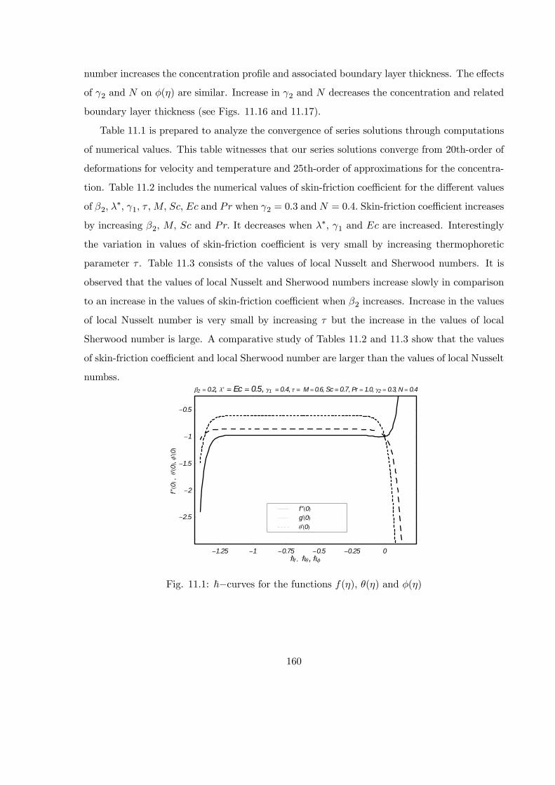
number increases the concentration profile and associated boundary layer thickness. The effects
of 2 and on () are similar. Increase in 2 and decreases the concentration and related
boundary layer thickness (see Figs. 11.16 and 11.17).
Table 11.1 is prepared to analyze the convergence of series solutions through computations
of numerical values. This table witnesses that our series solutions converge from 20th-order of
deformations for velocity and temperature and 25th-order of approximations for the concentra-
tion. Table 11.2 includes the numerical values of skin-friction coefficient for the different values
of 2 ∗ 1 and when 2 = 03 and = 04 Skin-friction coefficient increases
by increasing 2 and It decreases when ∗ 1 and are increased. Interestingly
the variation in values of skin-friction coefficient is very small by increasing thermophoretic
parameter . Table 11.3 consists of the values of local Nusselt and Sherwood numbers. It is
observed that the values of local Nusselt and Sherwood numbers increase slowly in comparison
to an increase in the values of skin-friction coefficient when 2 increases. Increase in the values
of local Nusselt number is very small by increasing but the increase in the values of local
Sherwood number is large. A comparative study of Tables 11.2 and 11.3 show that the values
of skin-friction coefficient and local Sherwood number are larger than the values of local Nusselt
numbss.
-1.25 -1 -0.75 -0.5 -0.25 0Ñf , Ñq , Ñf
-2.5
-2
-1.5
-1
-0.5
f''0
,q'0
,f'0
b2 = 0.2, l* = Ec = 0.5, g1 =0.4, t = M=0.6, Sc=0.7, Pr = 1.0, g2 = 0.3, N= 0.4
q'0g'0f''0
Fig. 11.1: ~−curves for the functions () () and ()
160
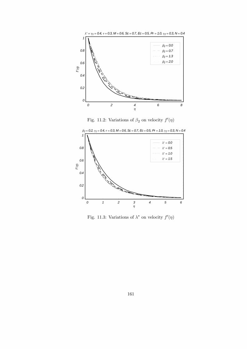
0 2 4 6 8h
0
0.2
0.4
0.6
0.8
1
f'h
l* = g1 = 0.4, t = 0.3, M = 0.6, Sc= 0.7, Ec= 0.5, Pr = 1.0, g2 = 0.3, N = 0.4
b2 = 2.0
b2 = 1.3
b2 = 0.7
b2 = 0.0
Fig. 11.2: Variations of 2 on velocity 0()
0 1 2 3 4 5 6h
0
0.2
0.4
0.6
0.8
1
f'h
b2 = 0.2, g1 = 0.4, t = 0.3, M = 0.6, Sc= 0.7, Ec= 0.5, Pr = 1.0, g2 = 0.3, N = 0.4
l* = 1.5
l* = 1.0
l* = 0.5
l* = 0.0
Fig. 11.3: Variations of ∗ on velocity 0()
161

0 1 2 3 4 5 6 7h
0
0.2
0.4
0.6
0.8
1
f'h
b2 = 0.2, l* = 0.4, t = 0.3, M = 0.6, Sc= 0.7, Ec= 0.5, Pr = 1.0, g2 = 0.3, N = 0.4
g1 = 1.2
g1 = 0.8
g1 = 0.4
g1 = 0.0
Fig. 11.4: Variations of 1 on velocity 0()
0 2 4 6 8h
0
0.2
0.4
0.6
0.8
1
f'h
b2 = 0.2, l* = g1 = 0.4, t = 0.3, Sc= 0.7, Ec = 0.5, Pr = 1.0, g2 = 0.3, N= 0.4
M= 1.2
M= 0.8
M= 0.4
M= 0.0
Fig. 11.5: Variations of on velocity 0()
162
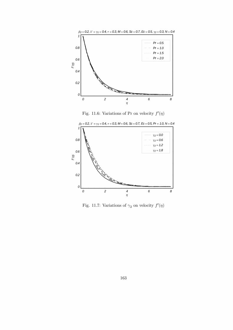
0 2 4 6 8h
0
0.2
0.4
0.6
0.8
1
f'h
b2 = 0.2, l* = g1 = 0.4, t = 0.3, M = 0.6, Sc= 0.7, Ec= 0.5, g2 = 0.3, N = 0.4
Pr = 2.0
Pr = 1.5
Pr = 1.0
Pr = 0.5
Fig. 11.6: Variations of Pr on velocity 0()
0 2 4 6 8h
0
0.2
0.4
0.6
0.8
1
f'h
b2 = 0.2, l* = g1 = 0.4, t = 0.3, M= 0.6, Sc= 0.7, Ec= 0.5, Pr = 1.0, N = 0.4
g2 = 1.8
g2 = 1.2
g2 = 0.6
g2 = 0.0
Fig. 11.7: Variations of 2 on velocity 0()
163
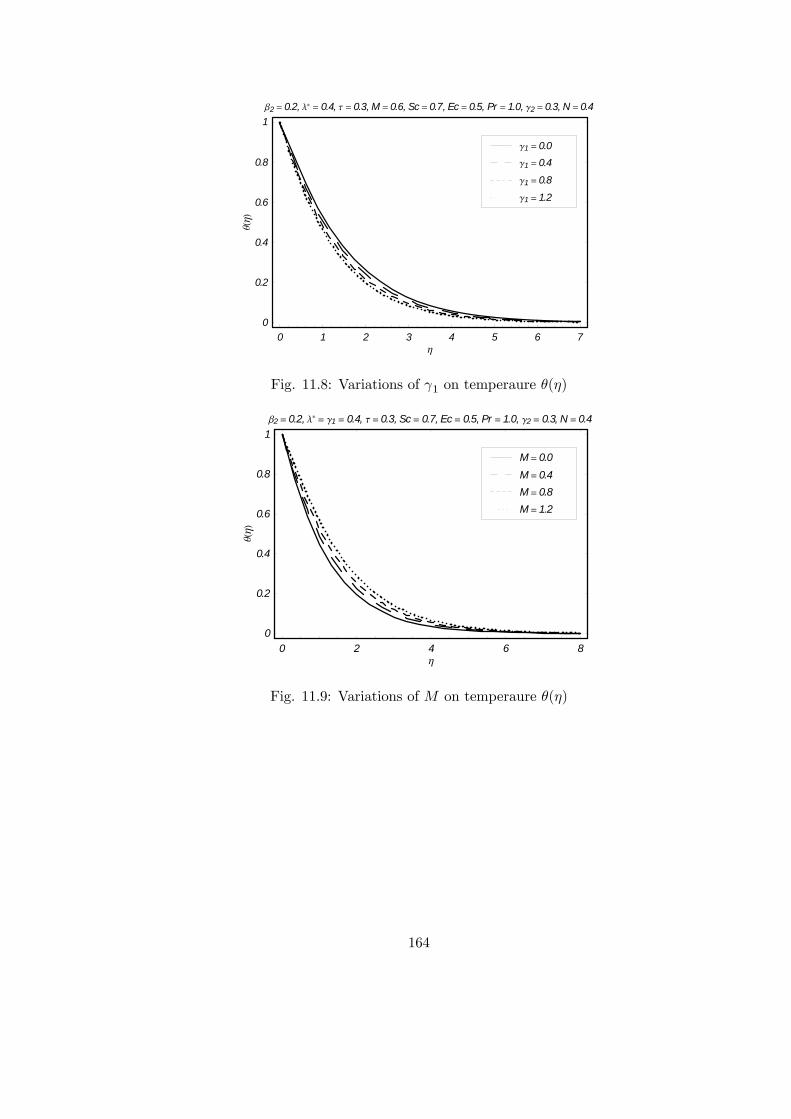
0 1 2 3 4 5 6 7h
0
0.2
0.4
0.6
0.8
1
qh
b2 = 0.2, l* = 0.4, t = 0.3, M = 0.6, Sc= 0.7, Ec= 0.5, Pr = 1.0, g2 = 0.3, N = 0.4
g1 = 1.2
g1 = 0.8
g1 = 0.4
g1 = 0.0
Fig. 11.8: Variations of 1 on temperaure ()
0 2 4 6 8h
0
0.2
0.4
0.6
0.8
1
qh
b2 = 0.2, l* = g1 = 0.4, t = 0.3, Sc= 0.7, Ec= 0.5, Pr = 1.0, g2 = 0.3, N = 0.4
M= 1.2
M= 0.8
M= 0.4
M= 0.0
Fig. 11.9: Variations of on temperaure ()
164

0 2 4 6 8h
0
0.2
0.4
0.6
0.8
1
qh
b2 = 0.2, l* = g1 = 0.4, t = 0.3, M= 0.6, Sc= 0.7, Pr = 1.0, g2 = 0.3, N = 0.4
Ec= 3.0
Ec= 2.0
Ec= 1.0
Ec= 0.0
Fig. 11.10: Variations of on temperaure ()
0 2 4 6 8h
0
0.2
0.4
0.6
0.8
1
qh
b2 = 0.2, l* = g1 = 0.4, t = 0.3, M= 0.6, Sc= 0.7, Ec= 0.5, g2 = 0.3, N = 0.4
Pr = 2.0
Pr = 1.5
Pr = 1.0
Pr = 0.5
Fig. 11.11: Variations of Pr on temperaure ()
165

0 2 4 6 8h
0
0.2
0.4
0.6
0.8
1
qh
b2 = 0.2, l* = g1 = 0.4, t = 0.3, M= 0.6, Sc= 0.7, Ec= 0.5, Pr = 1.0, N = 0.4
g2 = 1.8
g2 = 1.2
g2 = 0.6
g2 = 0.0
Fig. 11.12: Variations of 2 on temperaure ()
0 2 4 6 8h
0
0.2
0.4
0.6
0.8
1
qh
b2 = 0.2, l* = g1 = 0.4, t = 0.3, M = 0.6, Sc= 0.7, Ec= 0.5, Pr = 1.0, g2 = 0.3
N = 1.2
N = 0.8
N = 0.4
N = 0.0
Fig. 11.13: Variations of on temperaure ()
166
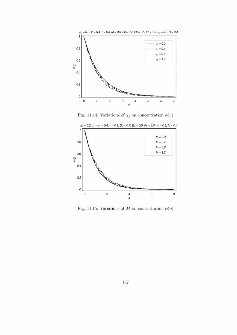
0 1 2 3 4 5 6 7h
0
0.2
0.4
0.6
0.8
1
fh
b2 = 0.2, l* = 0.4, t = 0.3, M= 0.6, Sc= 0.7, Ec= 0.5, Pr = 1.0, g2 = 0.3, N= 0.4
g1 = 1.2
g1 = 0.8
g1 = 0.4
g1 = 0.0
Fig. 11.14: Variations of 1 on concentration ()
0 2 4 6 8h
0
0.2
0.4
0.6
0.8
1
fh
b2 = 0.2, l* = g1 = 0.4, t = 0.3, Sc= 0.7, Ec= 0.5, Pr = 1.0, g2 = 0.3, N= 0.4
M= 1.2
M= 0.8
M= 0.4
M= 0.0
Fig. 11.15: Variations of on concentration ()
167
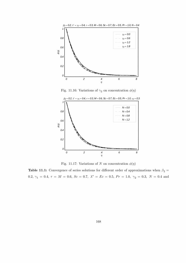
0 2 4 6 8h
0
0.2
0.4
0.6
0.8
1
fh
b2 = 0.2, l* = g1 = 0.4, t = 0.3, M = 0.6, Sc= 0.7, Ec= 0.5, Pr = 1.0, N = 0.4
g2 = 1.8
g2 = 1.2
g2 = 0.6
g2 = 0.0
Fig. 11.16: Variations of 2 on concentration ()
0 2 4 6 8h
0
0.2
0.4
0.6
0.8
1
fh
b2 = 0.2, l* = g1 = 0.4, t = 0.3, M = 0.6, Sc= 0.7, Ec= 0.5, Pr = 1.0, g2 = 0.3
N = 1.2
N = 0.8
N = 0.4
N = 0.0
Fig. 11.17: Variations of on concentration ()
Table 11.1: Convergence of series solutions for different order of approximations when 2 =
02 1 = 04 = = 06 = 07 ∗ = = 05 = 10 2 = 03 = 04 and
168
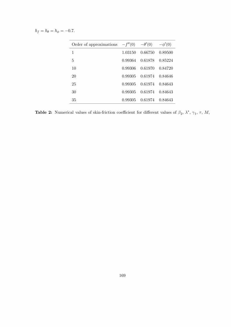
~ = ~ = ~ = −07
Order of approximations − 00(0) −0(0) −0(0)1 1.03150 0.66750 0.89500
5 0.99364 0.61878 0.85224
10 0.99306 0.61970 0.84720
20 0.99305 0.61974 0.84646
25 0.99305 0.61974 0.84643
30 0.99305 0.61974 0.84643
35 0.99305 0.61974 0.84643
Table 2: Numerical values of skin-friction coefficient for different values of 2 ∗ 1
169
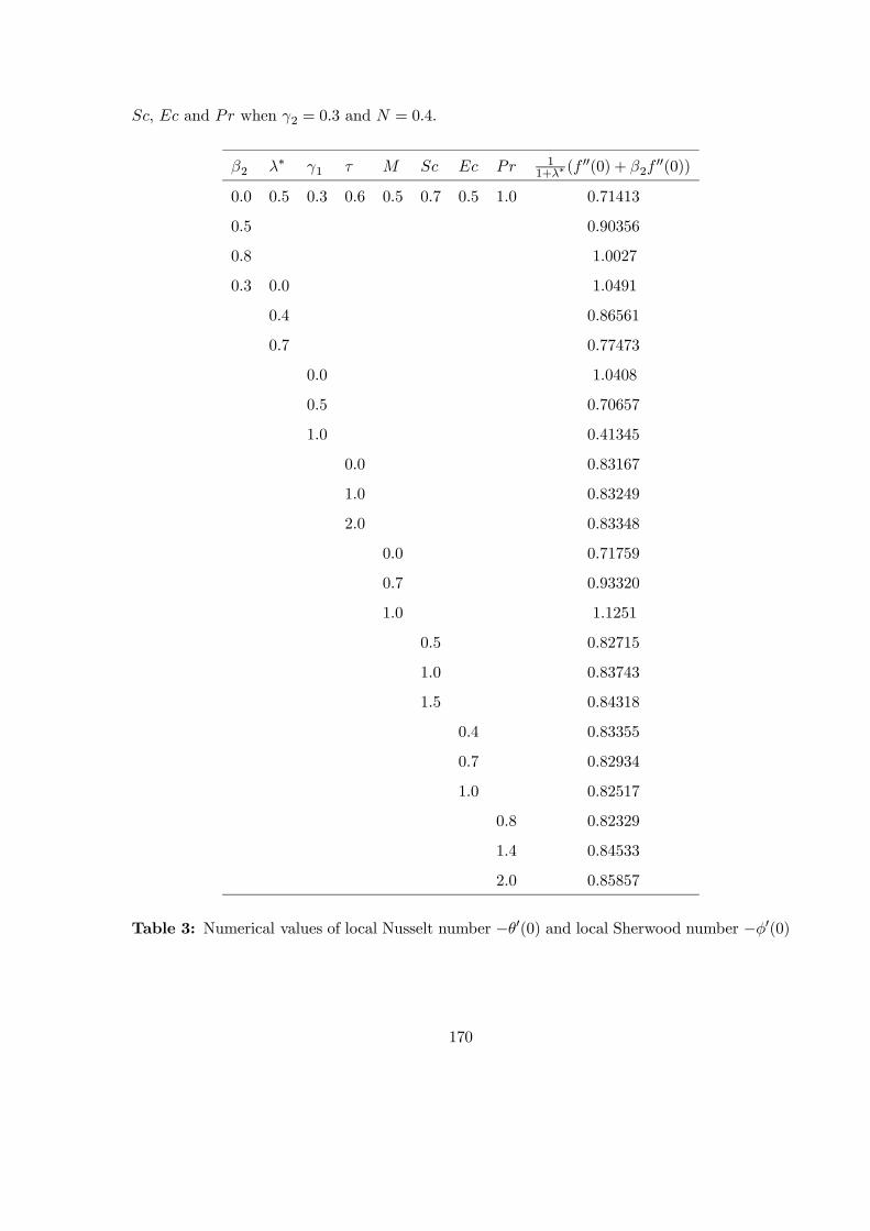
and when 2 = 03 and = 04
2 ∗ 1 11+∗ (
00(0) + 200(0))
00 05 03 06 05 07 05 10 071413
05 090356
08 10027
03 00 10491
04 086561
07 077473
00 10408
05 070657
10 041345
00 083167
10 083249
20 083348
00 071759
07 093320
10 11251
05 082715
10 083743
15 084318
04 083355
07 082934
10 082517
08 082329
14 084533
20 085857
Table 3: Numerical values of local Nusselt number −0(0) and local Sherwood number −0(0)
170

for different values of 2 ∗ 1 and when 2 = 03 and = 04
2 ∗ 1 −0(0) −0(0)00 05 03 06 05 07 05 10 059817 083428
05 064563 086222
08 066635 087576
03 00 067517 088177
04 063701 085682
07 061469 084353
00 051553 077548
05 067418 088124
10 074023 093082
00 062941 081539
10 062886 087961
20 062821 096235
00 070545 086946
07 056261 083748
10 043885 081203
05 063443 066407
10 062439 11064
15 062040 14825
04 065805 084409
07 057159 086747
10 048634 088986
08 055885 086466
14 074998 082693
20 089921 079074
171
11.4 Closing remarks
In this study we discussed the effects of thermal radiation, Joule heating and thermophoresis
in stretched flow of Jeffrey fluid. The main observations are as follows:
• Effects of 2 and ∗ on the fluid velocity are quite opposite.
• An increase in ratio of buoyancy parameter 2 corresponds to an increase in 0()
• The fluid temperature rises with an increase in Eckert number
• Effects of ratio of buoyancy and radiation parameters are qualitatively similar.
• Variations in temperature are more pronounced than that in concentration when in-
creases.
• Increase in the values of skin-friction coefficient and local Nusselt number is very small incomparison to an increase in local Sherwood number when increases.
• Numerical values of local Nusselt number increase and the values of local Sherwood num-ber decrease by increasing the Prandtl number
172
Chapter 12
Three-dimensional flow of Jeffrey
fluid with convective surface
boundary conditions
Three-dimensional flow of Jeffrey fluid over a stretched surface with convective boundary con-
dition is examined in this chapter. The equations governing this flow are modeled. The series
solutions of nonlinear equations are constructed. Results of velocity and temperature are ana-
lyzed. Further the numerical values of Nusselt number are computed and discussed. The present
analysis in a limiting sense is compared with the previous results. An excellent agreement is
noted.
12.1 Statement of the problems
We consider three-dimensional boundary layer flow of an incompressible Jeffrey fluid over a
stretching surface at = 0. The flow occupies the domain 0 We denote the ambient fluid
temperature by ∞. The surface temperature (to be determined later) is the result of convective
heating process which is characterized by a temperature and a heat transfer coefficient
The equations which can govern the flow in present situation are
+
+
= 0 (12.1)
173
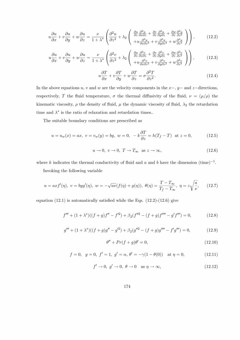
+
+
=
1 + ∗
⎛⎝2
2+ 2
⎛⎝
2
+
2
+
22
+ 32
+ 32
+ 33
⎞⎠⎞⎠ (12.2)
+
+
=
1 + ∗
⎛⎝2
2+ 2
⎛⎝
2
+
2
+
22
+ 32
+ 32
+ 33
⎞⎠⎞⎠ (12.3)
+
+
=
2
2 (12.4)
In the above equations and are the velocity components in the − − and −directions,respectively, the fluid temperature, the thermal diffusivity of the fluid, = () the
kinematic viscosity, the density of fluid, the dynamic viscosity of fluid, 2 the retardation
time and ∗ is the ratio of relaxation and retardation times..
The suitable boundary conditions are prescribed as
= () = = () = = 0 −
= ( − ) at = 0 (12.5)
→ 0 → 0 → ∞ as →∞ (12.6)
where indicates the thermal conductivity of fluid and and have the dimension (time)−1.
Invoking the following variable
= 0() = 0() = −√(() + ()) () = − ∞ − ∞
=
r
(12.7)
equation (12.1) is automatically satisfied while the Eqs. (12.2)-(12.6) give
000 + (1 + ∗)(( + ) 00 − 02) + 2(002 − ( + ) 0000 − 0 000) = 0 (12.8)
000 + (1 + ∗)(( + )00 − 02) + 2(002 − ( + )0000 − 0000) = 0 (12.9)
00 + ( + )0 = 0 (12.10)
= 0 = 0 0 = 1 0 = , 0 = −(1− (0)) at = 0 (12.11)
0 → 0 0 → 0 → 0 as →∞ (12.12)
174

where 2 = 2 is the Deborah number =is a ratio of stretching rates, =
is the
Prandtl number and =
pis the Biot number.
The local Nusselt number in non-dimensional form can be written as
12 = −0(0) (12.13)
in which = () is the local Reynolds number.
12.2 Homotopy analysis solutions
In order to proceed for homotopy analysis solutions, we write the following initial approxima-
tions and auxiliary linear operators
0() =¡1− −
¢ 0() =
¡1− −
¢ 0() =
exp(−)1 +
(12.14)
L = 000 − 0 L = 000 − 0 L = 00 − (12.15)
with
L (1 + 2 + 3
−) = 0 L(4 + 5 + 6
−) = 0 L(7 + 8−) = 0 (12.16)
where ( = 1− 8) are the arbitrary constants.The zeroth order problems can be expressed as
(1− )Lh(; )− 0()
i= ~N
h(; ) (; )
i (12.17)
(1− )L [(; )− 0()] = ~N
h(; ) (; )
i (12.18)
(1− )Lh(; )− 0()
i= ~N
h(; ) (; ) ( )
i (12.19)
(0; ) = 0 0(0; ) = 1 0(∞; ) = 0 (0; ) = 0 0(0; ) = 0(∞; ) = 0(12.20)
0(0 ) = −[1− (0 )] (∞ ) = 0 (12.21)
175
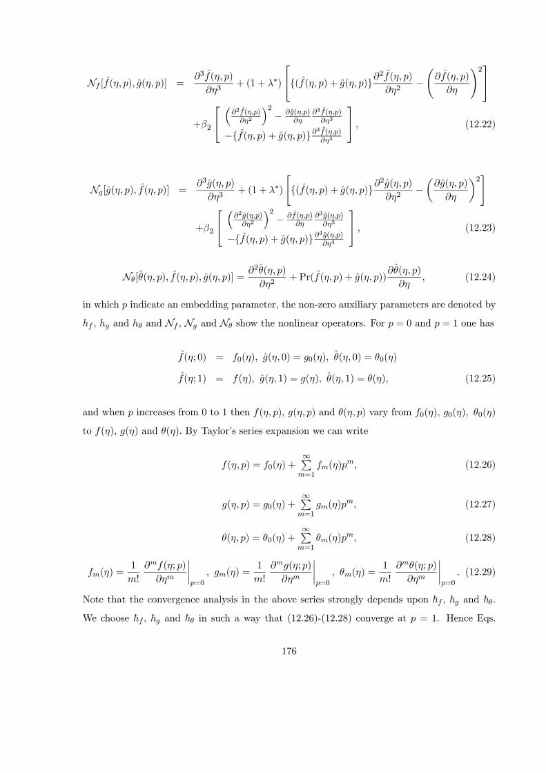
N [( ) ( )] =3( )
3+ (1 + ∗)
⎡⎣{(( ) + ( )}2( )
2−Ã( )
!2⎤⎦+2
⎡⎣ ³2()2
´2− ()
3()
3
−{( ) + ( )}4()4
⎤⎦ (12.22)
N[( ) ( )] =3( )
3+ (1 + ∗)
"{(( ) + ( )}
2( )
2−µ( )
¶2#
+2
⎡⎣ ³2()2
´2− ()
3()
3
−{( ) + ( )}4()4
⎤⎦ (12.23)
N[( ) ( ) ( )] =2( )
2+Pr(( ) + ( ))
( )
(12.24)
in which indicate an embedding parameter, the non-zero auxiliary parameters are denoted by
and and N N and N show the nonlinear operators. For = 0 and = 1 one has
(; 0) = 0() ( 0) = 0() ( 0) = 0()
(; 1) = () ( 1) = () ( 1) = () (12.25)
and when increases from 0 to 1 then ( ) ( ) and ( ) vary from 0() 0() 0()
to () () and () By Taylor’s series expansion we can write
( ) = 0() +∞P
=1
() (12.26)
( ) = 0() +∞P
=1
() (12.27)
( ) = 0() +∞P
=1
() (12.28)
() =1
!
(; )
¯=0
() =1
!
(; )
¯=0
() =1
!
(; )
¯=0
(12.29)
Note that the convergence analysis in the above series strongly depends upon ~ ~ and ~
We choose ~ ~ and ~ in such a way that (12.26)-(12.28) converge at = 1. Hence Eqs.
176
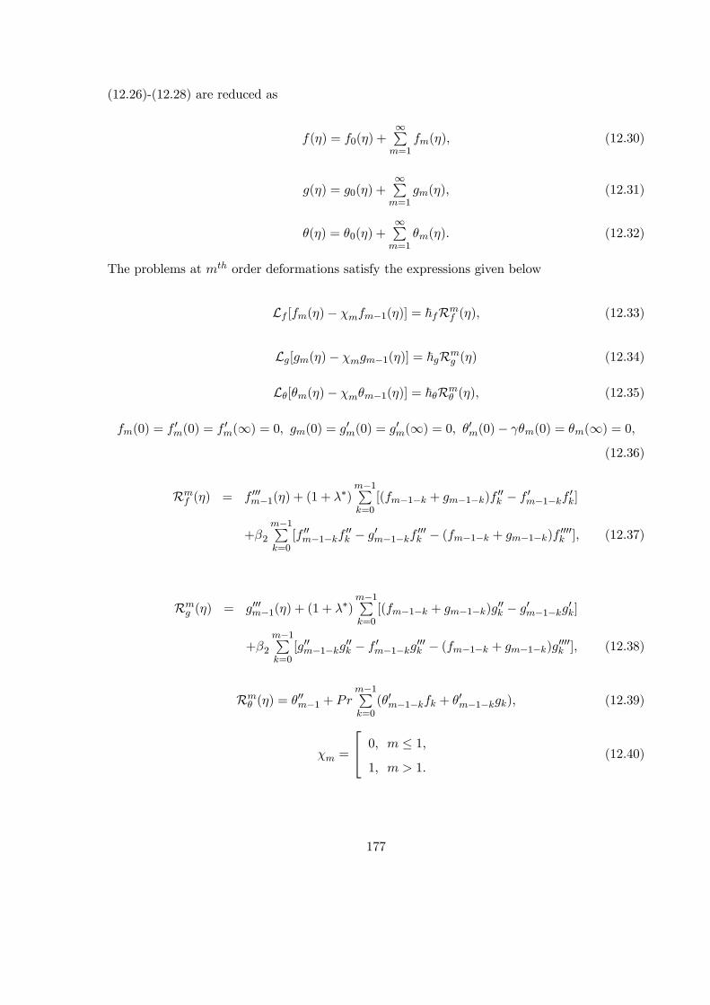
(12.26)-(12.28) are reduced as
() = 0() +∞P
=1
() (12.30)
() = 0() +∞P
=1
() (12.31)
() = 0() +∞P
=1
() (12.32)
The problems at order deformations satisfy the expressions given below
L [()− −1()] = ~R () (12.33)
L[()− −1()] = ~R () (12.34)
L[()− −1()] = ~R () (12.35)
(0) = 0(0) = 0(∞) = 0 (0) = 0(0) = 0(∞) = 0 0(0)− (0) = (∞) = 0(12.36)
R () = 000−1() + (1 + ∗)
−1P=0
[(−1− + −1−) 00 − 0−1−0]
+2
−1P=0
[ 00−1−00 − 0−1−
000 − (−1− + −1−) 0000 ] (12.37)
R () = 000−1() + (1 + ∗)
−1P=0
[(−1− + −1−)00 − 0−1−0]
+2
−1P=0
[00−1−00 − 0−1−
000 − (−1− + −1−)0000 ] (12.38)
R () = 00−1 +
−1P=0
(0−1− + 0−1−) (12.39)
=
⎡⎣ 0 ≤ 11 1
(12.40)
177

The general solutions can be expressed in the forms
() = ∗() + 1 + 2 +3
− (12.41)
() = ∗() + 4 + 5 + 6
− (12.42)
() = ∗() + 7 + 8
− (12.43)
where ∗ ∗ and ∗ are the special solutions.
12.3 Convergence of the homotopy solutions
Homotopy analysis method provides us a freedom to choose the auxiliary parameters ~ ~
and ~ to adjust and control the convergence of series solutions. Hence to find the appropriate
convergence region, we plotted the ~-curves at 21-order of approximations. It is found from
the Figs. 121−123 that the range of admissible values of ~ ~ and ~ are −09 ≤ } ≤ −02,−085 ≤ ~ ≤ −025 and −12 ≤ ~ ≤ −03. More our series solutions converge in the wholeregion of when ~ = ~ = −06 and ~ = −07
-1.2 -1 -0.8 -0.6 -0.4 -0.2 0Ñf
-1.125
-1.12
-1.115
-1.11
-1.105
-1.1
f''0
l* = 0.3, a = 0.4, b2 = 0.2
f ''0
Fig. 12.1: ~−curve for the function
178
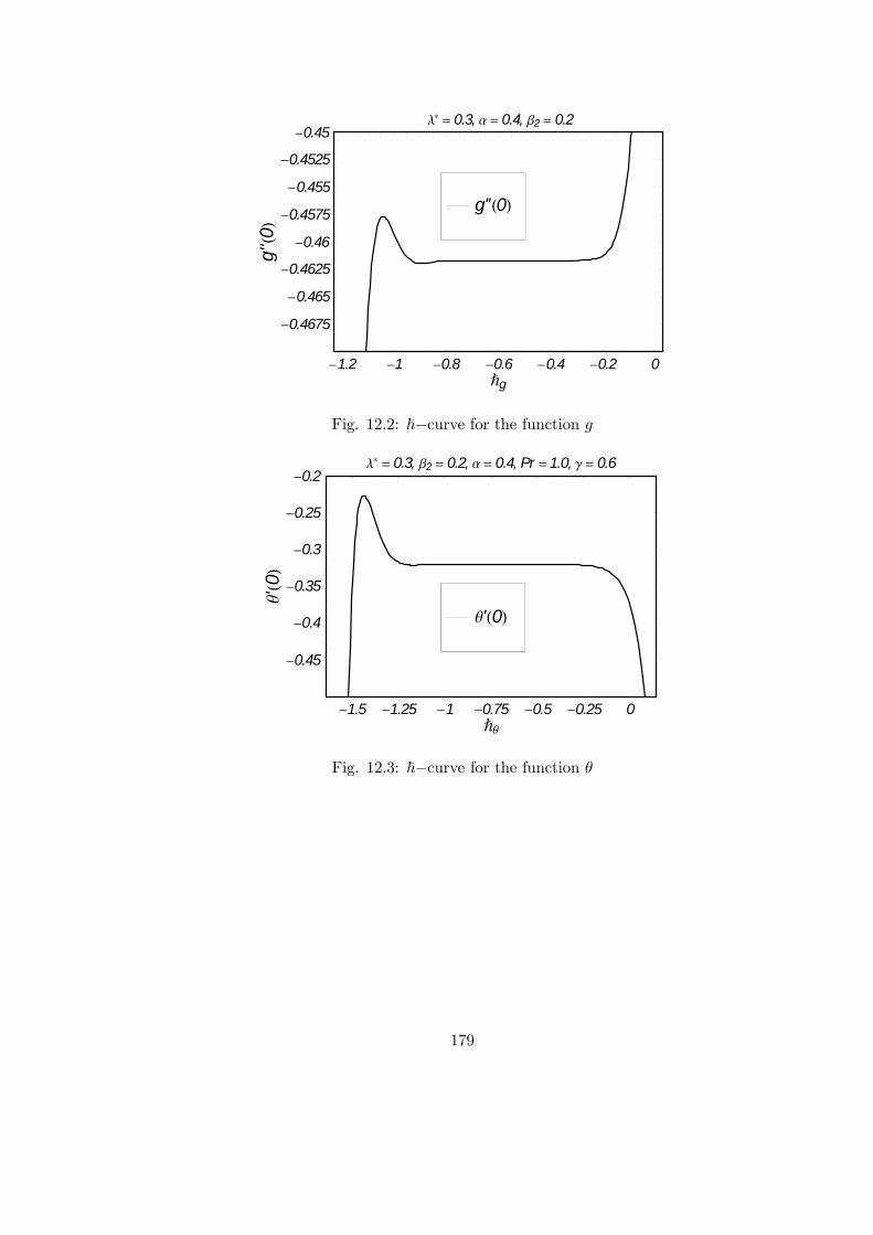
-1.2 -1 -0.8 -0.6 -0.4 -0.2 0Ñg
-0.4675
-0.465
-0.4625
-0.46
-0.4575
-0.455
-0.4525
-0.45
g''0
l* = 0.3, a= 0.4, b2 = 0.2
g''0
Fig. 12.2: ~−curve for the function
-1.5 -1.25 -1 -0.75 -0.5 -0.25 0Ñq
-0.45
-0.4
-0.35
-0.3
-0.25
-0.2
q'0
l* = 0.3, b2 = 0.2, a= 0.4, Pr =1.0, g = 0.6
q'0
Fig. 12.3: ~−curve for the function
179

Table: 12. 1. Convergence of homotopy solution for different order of approximations when
= 04 2 = 02 ∗ = 03 = 10, = 06 ~ = ~ = −06 and ~ = −07
Order of approximation − 00(0) −00(0) −0(0)1 1.090000 0.424000 0.348750
10 1.120311 0.461683 0.320161
20 1.120273 0.461715 0.319996
25 1.120274 0.461717 0.319996
30 1.120274 0.461717 0.319996
35 1.120274 0.461717 0.319996
12.4 Graphical results and discussion
The graphical results for various emerging parameters are discussed in this section. Figs.
124 − 1212 are plotted to see the variations of Deborah number 2 ratio of relaxation toretardation time ∗ the parameter Prandtl number and Biot number on the velocity
components 0() 0() and temperature () Fig. 12.4 depicts the influence of 2 on the
velocity 0() This Fig. clearly indicates that there is an increase in the boundary layer
thickness. It is due to the fact that 2 is dependent on the retardation time 2 The retardation
time increases the fluid velocity. The effects of ∗ and on 0() are seen in the Figs. 12.5
and 12.6. The velocity 0 decreases when ∗ and are increased. Figs. 12.7 − 129 show theinfluences of 2
∗ and on 0(). The effects of 2 and ∗ on 0() are quite similar to
that of 0() but the effect of on 0() is quite different. From Fig. 12.9 we observed that
the fluid velocity is zero when = 0 Further both the fluid velocity and thermal boundary
layer thickness increase when increases. The effects of Prandtl number on temperature
profile can be seen in Fig. 12.10. An increase in Prandtl number always decreases the thermal
boundary layer thickness and fluid temperature. Here we observed that the larger Prandtl
number fluids have lower thermal diffusivity and smaller Prandtl number fluids have stronger
thermal diffusivity. From Fig. 12.11 it can be seen that fluid temperature is zero for = 0
and increase in Biot number increases the fluid temperature. Biot number is dependent on
the heat transfer coefficient. This heat transfer coefficient has major role for the variation in
180
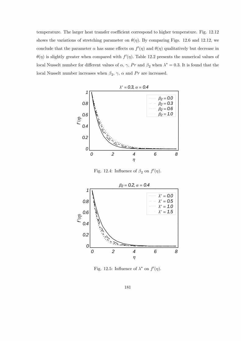
temperature. The larger heat transfer coefficient correspond to higher temperature. Fig. 12.12
shows the variations of stretching parameter on () By comparing Figs. 12.6 and 12.12, we
conclude that the parameter has same effects on 0() and () qualitatively but decrease in
() is slightly greater when compared with 0() Table 12.2 presents the numerical values of
local Nusselt number for different values of and 2 when ∗ = 03 It is found that the
local Nusselt number increases when 2 and are increased.
0 2 4 6 8h
0
0.2
0.4
0.6
0.8
1
f'h
l* = 0.3, a = 0.4
b2 = 1.0b2 = 0.6b2 = 0.3b2 = 0.0
Fig. 12.4: Influence of 2 on 0().
0 2 4 6 8h
0
0.2
0.4
0.6
0.8
1
f'h
b2 = 0.2, a = 0.4
l* = 1.5l* = 1.0l* = 0.5l* = 0.0
Fig. 12.5: Influence of ∗ on 0().
181
0 2 4 6 8h
0
0.2
0.4
0.6
0.8
1
f'h
b2= 0.2, l* = 0.3
a = 1.0a = 0.6a = 0.3a = 0.0
Fig. 12.6: Influence of on 0().
0 2 4 6 8h
0
0.1
0.2
0.3
0.4
g'h
l* = 0.3, a = 0.4
b2 = 1.0b2 = 0.6b2 = 0.3b2 = 0.0
Fig. 12.7: Influence of 2 on 0().
182
0 2 4 6 8h
0
0.1
0.2
0.3
0.4
g'h
b2 = 0.2, a = 0.4
l* = 1.5l* = 1.0l* = 0.5l* = 0.0
Fig. 12.8: Influence of ∗ on 0().
0 2 4 6 8h
0
0.2
0.4
0.6
0.8
1
g'h
b2= 0.2, l* = 0.3
a = 1.0a = 0.6a = 0.3a = 0.0
Fig. 12.9: Influence of on 0().
183
0 2 4 6 8 10h
0
0.1
0.2
0.3
0.4
0.5
qh
a = 0.4, g = 0.5, b2 = 0.2, l* = 0.3
Pr = 1.5Pr = 1.0Pr = 0.5Pr = 0.1
Fig. 12.10: Influence of on ().
0 2 4 6 8 10h
0
0.1
0.2
0.3
0.4
qh
Pr = 1.0, a = 0.4, b2 = 0.2, l* = 0.3
g = 0.6g = 0.4g = 0.2g = 0.0
Fig. 12.11: Influence of on ().
184
0 2 4 6 8 10h
0
0.1
0.2
0.3
0.4
qh
Pr = 0.7, a = 0.4, g = 0.2, l* = 0.3
b2 = 1.5b2 = 1.0b2 = 0.5b2 = 0.0
Fig. 12.12: Influence of 2 on ().
Table 12.2: Numerical values of −0(0) for different values of and 2 when ∗ = 03
2 −0(0)0.0 0.6 1.0 0.2 0.293238
0.3 0.313806
0.7 0.336750
1.0 0.351085
0.3 0.1 0.086805
0.4 0.248756
0.8 0.361009
1.3 0.436825
0.8 0.290453
1.2 0.332210
1.6 0.359781
2.0 0.379821
0.0 0.308166
0.3 0.315891
0.5 0.319381
0.7 0.322297
185

12.5 Concluding remarks
Effects of convective surface boundary condition in the three-dimensional flow of Jeffrey fluid
over a stretched surface are analyzed. The main observations are summarized in the following
points.
• Deborah number 2 and parameter ∗ have quite opposite effects on the velocity compo-nents 0() and 0()
• The velocity component 0() decreases while the velocity component 0() increases whenratio of stretching rates increases
• Increase in Prandtl number decreases the thermal boundary layer thickness and tem-perature.
• The Biot number increases the temperature.
• The local Nusselt number increases by increasing the Biot number.
186
Chapter 13
Three-dimensional flow of Jeffrey
fluid over a bidirectional stretching
surface with heat source/sink
This chapter provides generalization to the contents of previous chapter in the presence of vari-
able thermal conditions and heat source/sink. Two cases of heat transfer namely the prescribed
surface temperature (PST) and prescribed surface heat flux (PHF) are examined. Concept of
heat source/sink is employed. Homotopy analysis method (HAM) is adopted for the devel-
opment of series solutions. Limiting solutions available in the literature are deduced as the
special cases of the present results. Plots are prepared and discussed for the involved pertinent
parameters.
13.1 Heat transfer analysis
Consider three-dimensional boundary layer flow of an incompressible Jeffrey fluid induced by
bidirectional stretching surface (at = 0) with prescribed wall temperature and prescribed
surface heat flux. Flow of an incompressible fluid is considered for 0 The flow is considered
in the presence of heat source/sink parameter. The equations governing the present flow are
+
+
=
2
2+
( − ∞) (13.1)
187
where and are the velocity components in the − − and −directions, the fluid
temperature, the thermal diffusivity of the fluid, = () the kinematic viscosity, the
density of fluid, the dynamic viscosity of fluid, the specific heat at constant pressure of the
fluid and the heat source/sink parameter with 0 (heat source) and 0 (heat sink).
The boundary conditions corresponding to temperature are as follows.
Type I. Prescribed surface temperature (PST) [79,80]:
= ( ) = ∞ + at = 0
→ ∞ as →∞ (13.2)
Type II. Prescribed surface heat flux (PHF) [79,80]:
−
= at = 0
→ ∞ as →∞ (13.3)
In the above expressions is the thermal conductivity of the fluid, ∞ the constant temperature
outside the thermal boundary layer, and the positive constants. The power indices and
determine how the temperature or the heat flux varies in −plane.On setting
PST: () = ( )− ∞( )− ∞
PHF: ( )− ∞ =
r
() (13.4)
the above equations are reduced to the following forms:
00 + ( + )0 + ( − 0 − 0) = 0 (13.5)
00 + ( + )0 + ( − 0 − 0) = 0 (13.6)
= 1 0 = −1 at = 0
→ 0 → 0 as →∞ (13.7)
188
where = is the Prandtl number, the thermal diffusivity and =
the internal heat
parameter.
13.2 Homotopy analysis solutions
Initial approximations and auxiliary linear operators for the homotopy solutions are considered
in the following forms:
0() = exp(−) 0() = exp(−) (13.8)
L = 00 − L = 00 − (13.9)
with the properties
L(1 + 2−) = 0 L(3 + 4
−) = 0 (13.10)
where ( = 1− 4) are the arbitrary constants.The zeroth order problems can be constructed as follows:
(1− )Lh(; )− 0()
i= ~N
h(; ) (; ) ( )
i (13.11)
(1− )Lh(; )− 0()
i= ~N
h(; ) (; ) ( )
i (13.12)
(0; ) = 1 (∞ ) = 0 0(0 ) = 0 (∞ ) = 0 (13.13)
N[( ) ( ) ( )] =2( )
2+Pr(( ) + ( ))
( )
+Pr
à −
( )
−
( )
!( ) (13.14)
N[( ) ( ) ( )] =2( )
2+Pr(( ) + ( ))
( )
+Pr
à −
( )
−
( )
!( ) (13.15)
189

in which indicates the embedding parameter, the non-zero auxiliary parameters are denoted
by ~ and ~ and N and N show the nonlinear operators. For = 0 and = 1 we have
( 0) = 0() ( 0) = 0()
( 1) = () ( 1) = () (13.16)
and when increases from 0 to 1 then ( ) ( ) vary from 0() 0() to () and ()
By Taylor’s series expansion we have
( ) = 0() +∞P
=1
() (13.17)
( ) = 0() +∞P
=1
() (13.18)
() =1
!
(; )
¯=0
() =1
!
(; )
¯=0
(13.19)
The convergence analysis in the series strongly depends upon ~ and ~ We choose ~ and ~
in such a way that Eqs. (1317) and (1318) converge at = 1. Hence Eqs. (1317) and (1318)
give
() = 0() +∞P
=1
() (13.20)
() = 0() +∞P
=1
() (13.21)
The subjected problems for th order deformations are given by
L[()− −1()] = ~R () (13.22)
L[()− −1()] = ~R () (13.23)
(0) = (∞) = 0 0(0) = (∞) = 0 (13.24)
R () = 00−1 +
−1P=0
(0−1− + 0−1−) + −1()
−−1P=0
0−1− − −1P=0
0−1− (13.25)
190
R () = 00−1 +
−1P=0
(0−1− + 0−1−) + −1()
−−1P=0
0−1− − −1P=0
0−1− (13.26)
=
⎡⎣ 0 ≤ 11 1
(13.27)
The general solutions can be expressed in the forms
() = ∗() + 7 + 8
− (13.28)
() = ∗() +9 + 10
− (13.29)
where ∗ and ∗ are the special solutions.
13.3 Convergence of the homotopy solutions
Homotopy analysis method provides us a freedom about the selection of the auxiliary parameters
~ and ~ in order to adjust and control the convergence of series solutions. Hence to find the
appropriate convergence region, we have plotted the ~−curves at 24-order of approximations.It is found from the Figs. 1 and 2 that the range of admissible values of ~ and ~ are
191
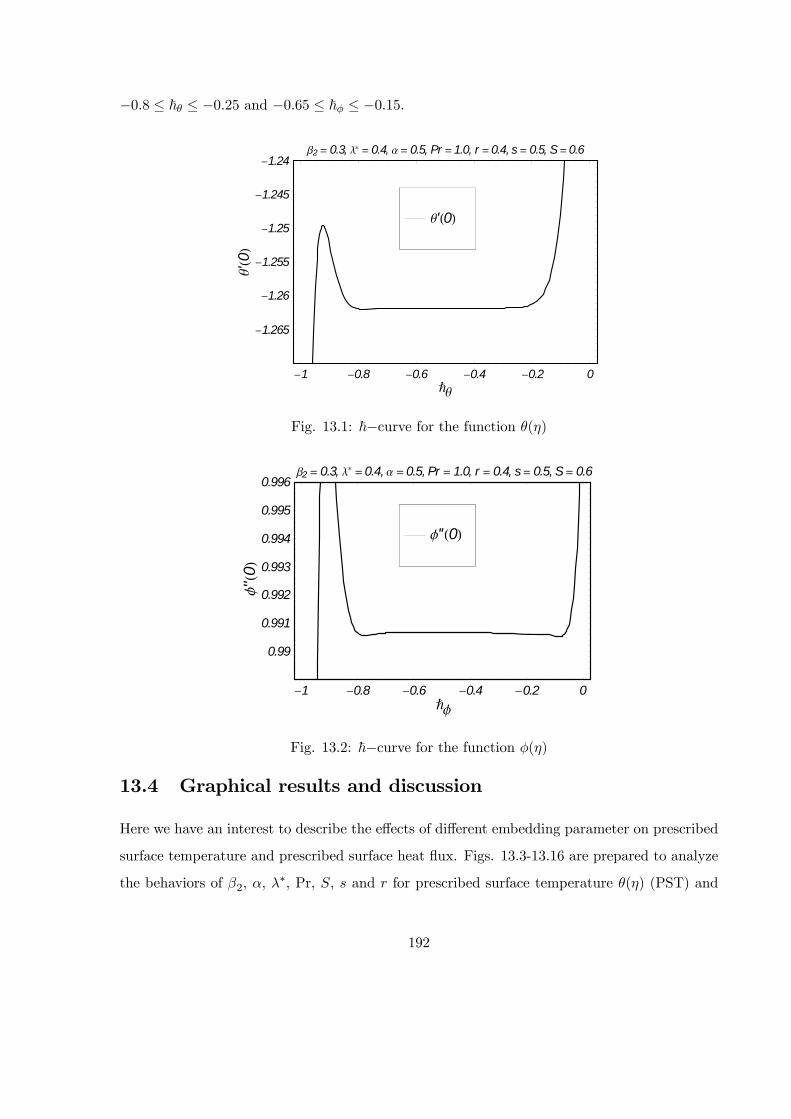
−08 ≤ ~ ≤ −025 and −065 ≤ ~ ≤ −015
-1 -0.8 -0.6 -0.4 -0.2 0Ñq
-1.265
-1.26
-1.255
-1.25
-1.245
-1.24
q'0
b2 = 0.3, l* = 0.4, a= 0.5, Pr =1.0, r =0.4, s= 0.5, S=0.6
q'0
Fig. 13.1: ~−curve for the function ()
-1 -0.8 -0.6 -0.4 -0.2 0Ñf
0.99
0.991
0.992
0.993
0.994
0.995
0.996
f''0
b2 = 0.3, l* =0.4, a =0.5, Pr = 1.0, r = 0.4, s= 0.5, S= 0.6
f''0
Fig. 13.2: ~−curve for the function ()
13.4 Graphical results and discussion
Here we have an interest to describe the effects of different embedding parameter on prescribed
surface temperature and prescribed surface heat flux. Figs. 13.3-13.16 are prepared to analyze
the behaviors of 2, , ∗, Pr, , and for prescribed surface temperature () (PST) and
192

prescribed surface heat flux () (PHF). The Deborah number 2 has similar effects for PST
and PHF in a qualitative sense. An increase in 2 corresponds to a decrease in PST and PHF
cases. The variations in PHF are significant in comparison to the variation in PST (see Figs.
13.3 and 13.4). Furthermore this decrease is due to an increase in retardation time. Figs. 13.5
and 13.6 analyzed that both () and () are decreasing functions of . The thermal boundary
layer thickness for PST and PHF cases are reduced with an increase in . Figs. 13.7 and 13.8
show that the boundary layer thickness increase by increasing ∗. Effects of Prandtl number
Pr are seen in the Figs. 13.9 and 13.10. These Figs. depict that temperatures in both the
PST and PHF cases are decreasing functions of Prandtl number. This occurs due to the fact
that an increase in Pr corresponds to a lower thermal diffusivity due to which such decrease
arises. The heat generation parameter gives rise to the temperatures in PST and PHF cases
(see Figs. 13.11 and 13.12). This is due to the fact that heat generation creates the thicker
thermal boundary layer. Figs. 13.13 and 13.14 depict that (), () and their boundary layer
thickness reduce with an increase in . Also we noted that the decrease in PHF is larger in
comparison to a decrease for PST case. The values of () and () are decreasing functions of
. Also such decrease in PHF case is more dominant (see Figs. 13.15 and 13.16). The effects of
power indices and on local Nusselt number −0(0) are seen in Fig. 13.17. The local Nusseltnumber increases by increasing and The local Nusselt number is an increasing function of
ratio parameter and Prandtl number (see Fig. 13.18). Fig. 13.19 shows that an increase in
and 2 leads to an increase in the local Nusselt number. Tables 1 and 2 are computed for
the values correspond to the different values of in a limiting case. From these Tables, we
have seen that our series solutions have a complete agreement with the previous solutions for
193
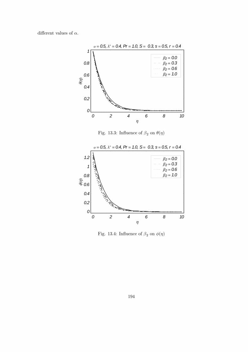
different values of
0 2 4 6 8 10h
0
0.2
0.4
0.6
0.8
1
qh
a = 0.5, l* = 0.4, Pr = 1.0, S= 0.3, s = 0.5, r = 0.4
b2 = 1.0b2 = 0.6b2 = 0.3b2 = 0.0
Fig. 13.3: Influence of 2 on ()
0 2 4 6 8 10h
0
0.2
0.4
0.6
0.8
1
1.2
fh
a = 0.5, l* = 0.4, Pr = 1.0, S= 0.3, s= 0.5, r = 0.4
b2 = 1.0b2 = 0.6b2 = 0.3b2 = 0.0
Fig. 13.4: Influence of 2 on ()
194
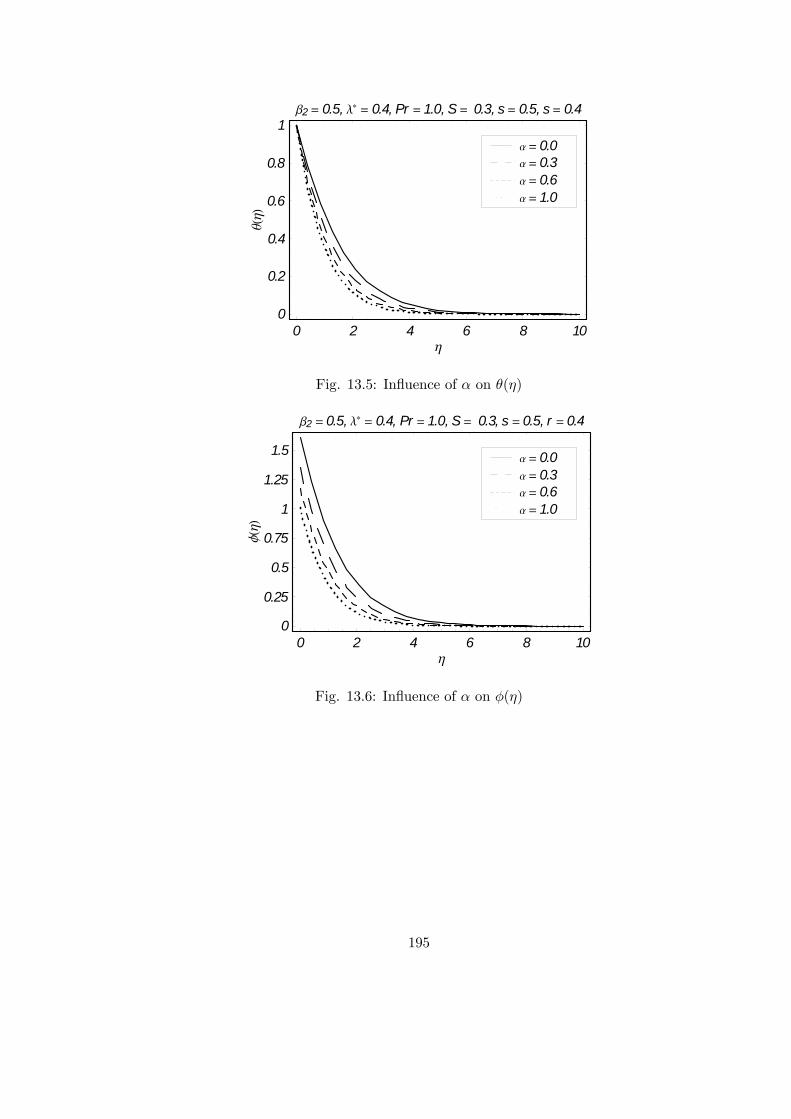
0 2 4 6 8 10h
0
0.2
0.4
0.6
0.8
1
qh
b2 = 0.5, l* = 0.4, Pr = 1.0, S= 0.3, s= 0.5, s= 0.4
a = 1.0a = 0.6a = 0.3a = 0.0
Fig. 13.5: Influence of on ()
0 2 4 6 8 10h
0
0.25
0.5
0.75
1
1.25
1.5
fh
b2 = 0.5, l* = 0.4, Pr = 1.0, S= 0.3, s = 0.5, r = 0.4
a = 1.0a = 0.6a = 0.3a = 0.0
Fig. 13.6: Influence of on ()
195

0 2 4 6 8 10h
0
0.2
0.4
0.6
0.8
1
qh
b2 = 0.5, a = 0.4, Pr = 1.0, S= 0.3, s= 0.5, r = 0.4
l* = 1.5l* = 1.0l* = 0.5l* = 0.0
Fig. 13.7: Influence of ∗ on ()
0 2 4 6 8 10h
0
0.2
0.4
0.6
0.8
1
1.2
1.4
fh
b2 = 0.5, a = 0.4, Pr = 1.0, S= 0.3, s= 0.5, r = 0.4
l* = 1.5l* = 1.0l* = 0.5l* = 0.0
Fig. 13.8: Influence of ∗ on ()
196
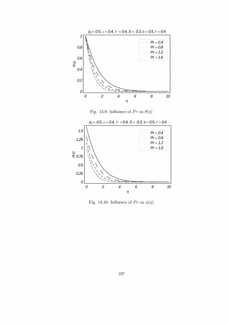
0 2 4 6 8 10h
0
0.2
0.4
0.6
0.8
1
qh
b2 = 0.5, a = 0.4, l* = 0.4, S= 0.3, s= 0.5, r = 0.4
Pr = 1.6Pr = 1.2Pr = 0.8Pr = 0.4
Fig. 13.9: Influence of on ()
0 2 4 6 8 10h
0
0.25
0.5
0.75
1
1.25
1.5
fh
b2 = 0.5, a = 0.4, l* = 0.4, S= 0.3, s= 0.5, r = 0.4
Pr = 1.6Pr = 1.2Pr = 0.8Pr = 0.4
Fig. 13.10: Influence of on ()
197
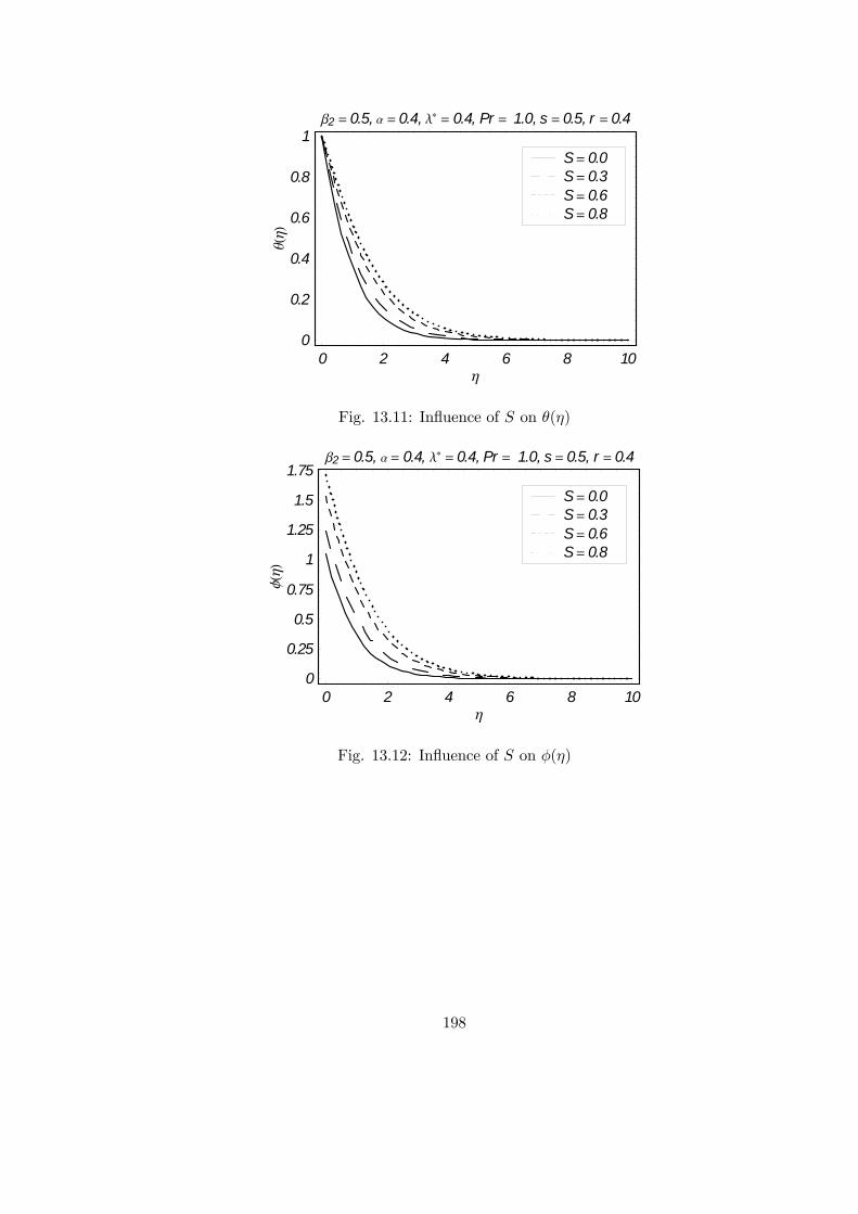
0 2 4 6 8 10h
0
0.2
0.4
0.6
0.8
1
qh
b2 = 0.5, a = 0.4, l* = 0.4, Pr = 1.0, s = 0.5, r = 0.4
S= 0.8S= 0.6S= 0.3S= 0.0
Fig. 13.11: Influence of on ()
0 2 4 6 8 10h
0
0.25
0.5
0.75
1
1.25
1.5
1.75
fh
b2 = 0.5, a = 0.4, l* = 0.4, Pr = 1.0, s= 0.5, r = 0.4
S= 0.8S= 0.6S= 0.3S= 0.0
Fig. 13.12: Influence of on ()
198

0 2 4 6 8 10h
0
0.2
0.4
0.6
0.8
1
qh
b2 = 0.5, a = 0.4, l* = 0.4, Pr = 1.0, S= 0.3, r = 0.4
s= 1.5s= 1.0s= 0.5s= 0.0
Fig. 13.13: Influence of on ()
0 2 4 6 8 10h
0
0.2
0.4
0.6
0.8
1
1.2
1.4
fh
b2 = 0.5, a = 0.4, l* = 0.4, Pr = 1.0, S= 0.3, r = 0.4
s= 1.5s= 1.0s= 0.5s= 0.0
Fig. 13.14: Influence of on ()
199
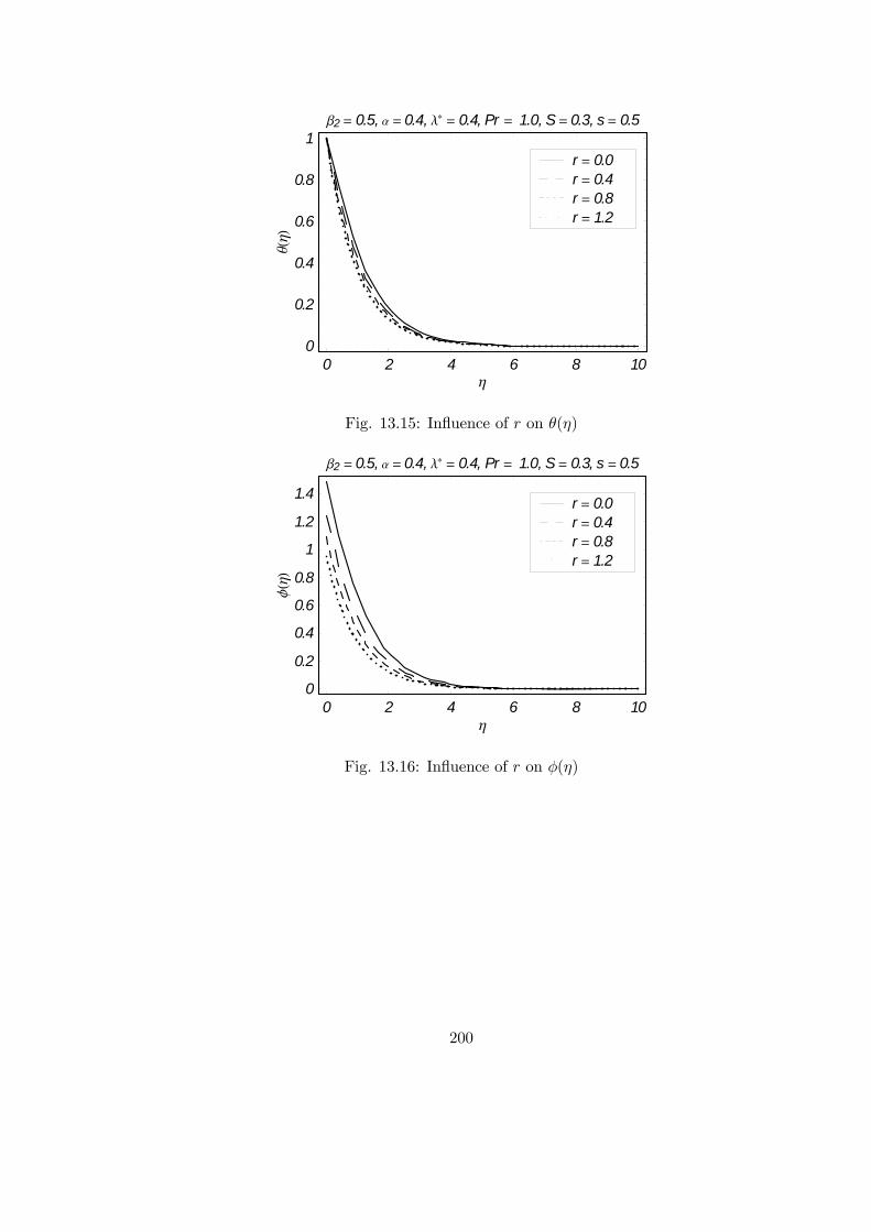
0 2 4 6 8 10h
0
0.2
0.4
0.6
0.8
1
qh
b2 = 0.5, a = 0.4, l* = 0.4, Pr = 1.0, S= 0.3, s= 0.5
r = 1.2r = 0.8r = 0.4r = 0.0
Fig. 13.15: Influence of on ()
0 2 4 6 8 10h
0
0.2
0.4
0.6
0.8
1
1.2
1.4
fh
b2 = 0.5, a = 0.4, l* = 0.4, Pr = 1.0, S= 0.3, s = 0.5
r = 1.2r = 0.8r = 0.4r = 0.0
Fig. 13.16: Influence of on ()
200
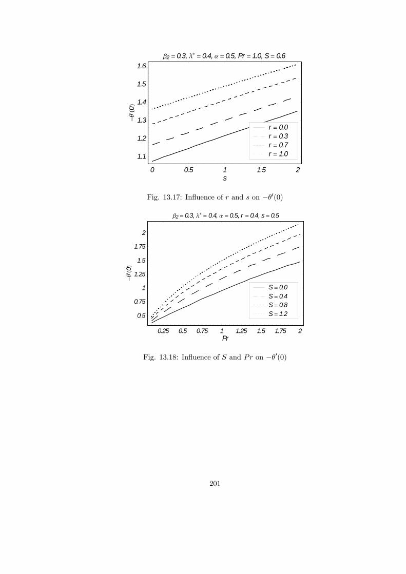
0 0.5 1 1.5 2s
1.1
1.2
1.3
1.4
1.5
1.6
-q'
0
b2 = 0.3, l* = 0.4, a = 0.5, Pr = 1.0, S= 0.6
r = 1.0r = 0.7r = 0.3r = 0.0
Fig. 13.17: Influence of and on −0(0)
0.25 0.5 0.75 1 1.25 1.5 1.75 2Pr
0.5
0.75
1
1.25
1.5
1.75
2
-q'
0
b2 = 0.3, l* = 0.4, a = 0.5, r = 0.4, s= 0.5
S= 1.2S= 0.8S= 0.4S= 0.0
Fig. 13.18: Influence of and on −0(0)
201

0 0.5 1 1.5 2b2
1.15
1.2
1.25
1.3
1.35
1.4
1.45
-q'
0
l* = 0.4, Pr = 1.0, r = 0.4, s= 0.5, S= 0.6
a = 1.0a = 0.7a = 0.4a = 0.1
Fig. 13.19: Influence of and on −0(0)Table 13.2: Numerical values of 00(0) 00(0) (∞) and (∞) for different values of
when 1 = 1 = 0
Wang [25] Present results
00(0) 00(0) (∞) (∞) 00(0) 00(0) (∞) (∞)0.0 -1 0 1 0 -1 0 1 0
0.25 -1.048813 -0.194564 0.907075 0.257986 -1.04881 -0.19457 0.907047 0.25790
0.50 -1.093097 -0.465205 0.842360 0.451671 -109309 -0.46522 0.84293 0.45169
0.75 -1.134485 -0.794622 0.792308 0.612049 -1.13450 -0.79462 0.79231 0.61214
1.0 -1.173720 -1.173720 0.751527 0.751527 -1.17372 -1.17372 0.75149 0.75149
13.5 Concluding remarks
Effects of prescribed surface temperature and prescribed surface heat flux in three-dimensional
flow of Jeffrey fluid is discussed in the presence of heat source/sink. The main observations are
as follows.
• The prescribed surface temperature and prescribed surface heat flux are decreasing func-tions of
• The variations in prescribed surface heat flux are more dominant when compared with
202
that of prescribed surface temperature.
• Both PST and PHF are reduced when we increase the values of Pr
• An increase in the values of leads to a decrease in both PST and PHF.
203
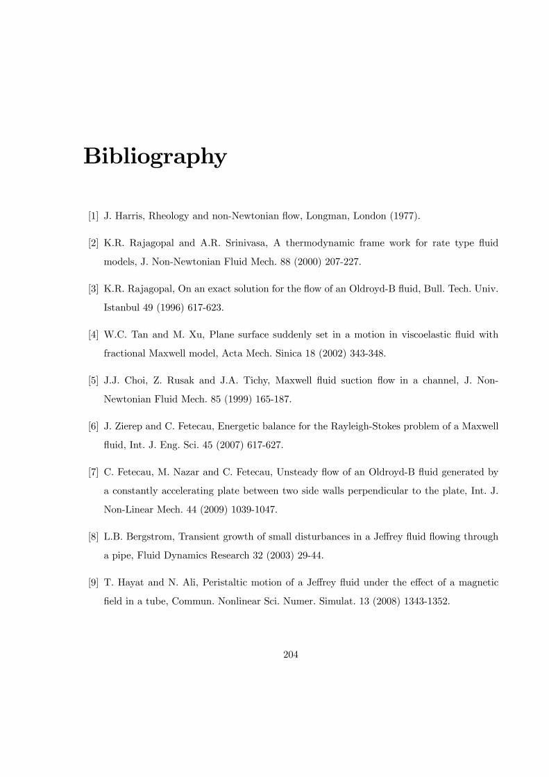
Bibliography
[1] J. Harris, Rheology and non-Newtonian flow, Longman, London (1977).
[2] K.R. Rajagopal and A.R. Srinivasa, A thermodynamic frame work for rate type fluid
models, J. Non-Newtonian Fluid Mech. 88 (2000) 207-227.
[3] K.R. Rajagopal, On an exact solution for the flow of an Oldroyd-B fluid, Bull. Tech. Univ.
Istanbul 49 (1996) 617-623.
[4] W.C. Tan and M. Xu, Plane surface suddenly set in a motion in viscoelastic fluid with
fractional Maxwell model, Acta Mech. Sinica 18 (2002) 343-348.
[5] J.J. Choi, Z. Rusak and J.A. Tichy, Maxwell fluid suction flow in a channel, J. Non-
Newtonian Fluid Mech. 85 (1999) 165-187.
[6] J. Zierep and C. Fetecau, Energetic balance for the Rayleigh-Stokes problem of a Maxwell
fluid, Int. J. Eng. Sci. 45 (2007) 617-627.
[7] C. Fetecau, M. Nazar and C. Fetecau, Unsteady flow of an Oldroyd-B fluid generated by
a constantly accelerating plate between two side walls perpendicular to the plate, Int. J.
Non-Linear Mech. 44 (2009) 1039-1047.
[8] L.B. Bergstrom, Transient growth of small disturbances in a Jeffrey fluid flowing through
a pipe, Fluid Dynamics Research 32 (2003) 29-44.
[9] T. Hayat and N. Ali, Peristaltic motion of a Jeffrey fluid under the effect of a magnetic
field in a tube, Commun. Nonlinear Sci. Numer. Simulat. 13 (2008) 1343-1352.
204
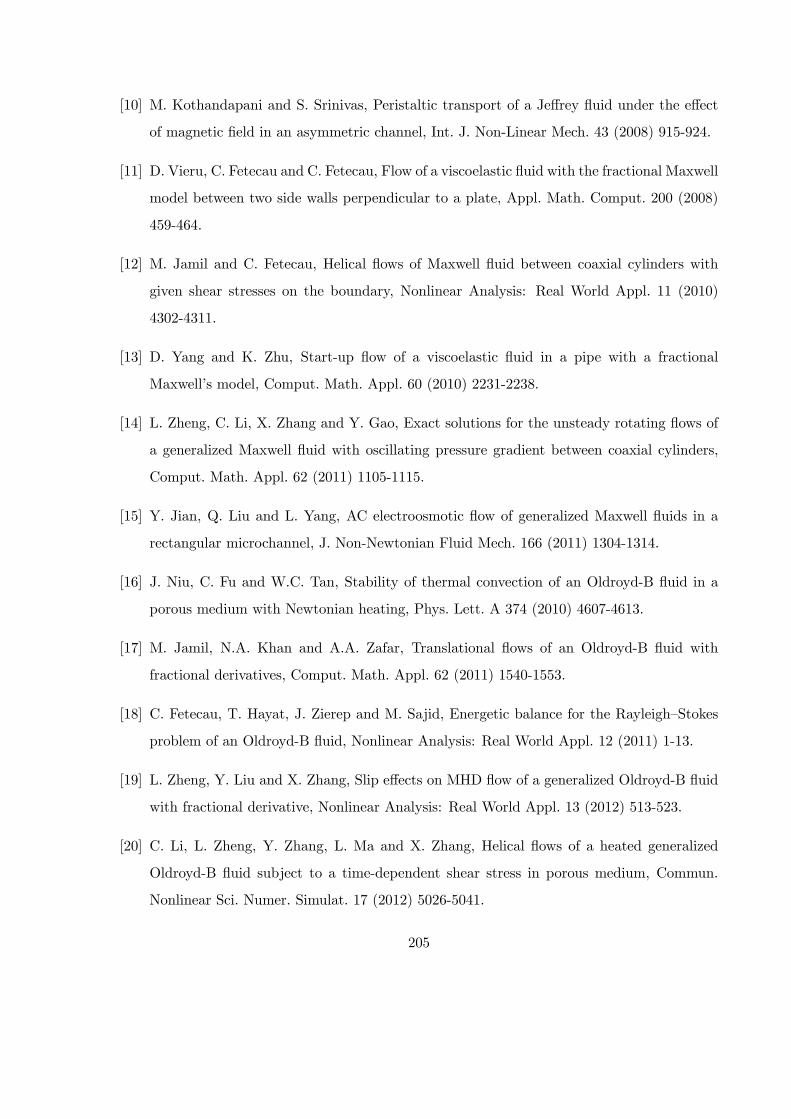
[10] M. Kothandapani and S. Srinivas, Peristaltic transport of a Jeffrey fluid under the effect
of magnetic field in an asymmetric channel, Int. J. Non-Linear Mech. 43 (2008) 915-924.
[11] D. Vieru, C. Fetecau and C. Fetecau, Flow of a viscoelastic fluid with the fractional Maxwell
model between two side walls perpendicular to a plate, Appl. Math. Comput. 200 (2008)
459-464.
[12] M. Jamil and C. Fetecau, Helical flows of Maxwell fluid between coaxial cylinders with
given shear stresses on the boundary, Nonlinear Analysis: Real World Appl. 11 (2010)
4302-4311.
[13] D. Yang and K. Zhu, Start-up flow of a viscoelastic fluid in a pipe with a fractional
Maxwell’s model, Comput. Math. Appl. 60 (2010) 2231-2238.
[14] L. Zheng, C. Li, X. Zhang and Y. Gao, Exact solutions for the unsteady rotating flows of
a generalized Maxwell fluid with oscillating pressure gradient between coaxial cylinders,
Comput. Math. Appl. 62 (2011) 1105-1115.
[15] Y. Jian, Q. Liu and L. Yang, AC electroosmotic flow of generalized Maxwell fluids in a
rectangular microchannel, J. Non-Newtonian Fluid Mech. 166 (2011) 1304-1314.
[16] J. Niu, C. Fu and W.C. Tan, Stability of thermal convection of an Oldroyd-B fluid in a
porous medium with Newtonian heating, Phys. Lett. A 374 (2010) 4607-4613.
[17] M. Jamil, N.A. Khan and A.A. Zafar, Translational flows of an Oldroyd-B fluid with
fractional derivatives, Comput. Math. Appl. 62 (2011) 1540-1553.
[18] C. Fetecau, T. Hayat, J. Zierep and M. Sajid, Energetic balance for the Rayleigh—Stokes
problem of an Oldroyd-B fluid, Nonlinear Analysis: Real World Appl. 12 (2011) 1-13.
[19] L. Zheng, Y. Liu and X. Zhang, Slip effects on MHD flow of a generalized Oldroyd-B fluid
with fractional derivative, Nonlinear Analysis: Real World Appl. 13 (2012) 513-523.
[20] C. Li, L. Zheng, Y. Zhang, L. Ma and X. Zhang, Helical flows of a heated generalized
Oldroyd-B fluid subject to a time-dependent shear stress in porous medium, Commun.
Nonlinear Sci. Numer. Simulat. 17 (2012) 5026-5041.
205
[21] B.C. Sakiadis, Boundary layer behavior on continuous solid surfaces: II Boundary on a
continuous flat surface, AIChE J. 7 (1961) 221-225.
[22] L.J. Crane, Flow past a stretching plate, Z. Angew. Math. Phys. 21 (1970) 645-647.
[23] J.B. McLeod and K.R. Rajagopal, On the uniqueness of flow of Navier-Stokes fluid due to
a stretching boundary, Arch. Rat. Mech. Anal. 98 (1987) 385-393.
[24] C.Y. Wang, Stretching surface in a rotating fluid, J. Appl. Phys. 39 (1988) 177-185.
[25] C.Y. Wang, The three-dimensional flow due to stretching surface, Phys. Fluids 27 (1984)
1915-1917.
[26] V. Rajeswari and G. Nath, Unsteady flow over a stretching surface in a rotating fluid, Int.
J. Eng. Sci. 30 (1992) 747-756.
[27] P.D. Ariel, Axisymmetric flow due to a stretching sheet with partial slip, Comput. Math.
Appl. 54 (2007) 1169-1183.
[28] P.D. Ariel, Axisymmetric flow of a second grade fluid past a stretching sheet, Int. J. Eng.
Sci. 39 (2001) 529-553.
[29] P.D. Ariel, The three-dimensional flow past a stretching sheet and the homotopy pertur-
bation method, Comput. Math. Appl. 54 (2007) 920-925.
[30] T.R. Mahapatra, S. Dholey and A.S. Gupta, Oblique stagnation-point flow of an incom-
pressible visco-elastic fluid towards a stretching surface, Int. J. Non-Linear Mech. 42 (2007)
484-499.
[31] S.J. Liao, A new branch of solutions of boundary-layer flows over a permeable stretching
plate, Int. J. Non-Linear Mech. 42 (2007) 819-830.
[32] T. Hayat, M. Sajid and I. Pop, Three-dimensional flow over a stretching surface in a
viscoelastic fluid, Nonlinear Analysis: Real World Appl. 9 (2008) 1811-1822.
[33] M. Ayub, H. Zaman, M. Sajid and T. Hayat, Analytical solution of stagnation-point flow of
a viscoelastic fluid towards a stretching surface, Commun. Nonlinear Sci. Numer. Simulat.
13 (2008) 1822-1835.
206

[34] Z. Abbas, Y. Wang, T. Hayat and M. Oberlack, Hydromagnetic flow in a viscoelastic fluid
due to the oscillatory stretching surface, Int. J. Non-Linear Mech. 43 (2008) 783-793.
[35] T. Ray Mahapatra, S.K. Nandy and A.S. Gupta, Magnetohydrodynamic stagnation-point
flow of a power-law fluid towards a stretching surface, Int. J. Non-Linear Mech. 44 (2009)
124-129.
[36] T. Hayat, T. Javed and Z. Abbas, MHD flow of a micropolar fluid near a stagnation-point
towards a non-linear stretching surface, Nonlinear Analysis: Real World Appl. 10 (2009)
1514-1526.
[37] S. Aïboud and S. Saouli, Entropy analysis for viscoelastic magnetohydrodynamic flow over
a stretching surface, Int. J. Non-Linear Mech. 45 (2010) 482-489.
[38] B.S. Dandapat and S. Chakraborty, Effects of variable fluid properties on unsteady thin-
film flow over a non-linear stretching sheet, Int. J. Heat Mass Transfer 53 (2010) 5757-5763.
[39] F.T. Akyildiz, H. Bellout, K. Vajravelu and R.A. Van Gorder, Existence results for third
order nonlinear boundary value problems arising in nano boundary layer fluid flows over
stretching surfaces, Nonlinear Analysis: Real World Appl.12 (2011) 2919-2930.
[40] A. Ahmad and S. Asghar, Flow of a second grade fluid over a sheet stretching with arbitrary
velocities subject to a transverse magnetic field, Appl. Math. Letters 24 (2011) 1905-1909.
[41] A.J. Chamkha, Effects of heat absorption and thermal radiation on heat transfer in a
fluid—particle flow past a surface in the presence of a gravity field, Int. J. Thermal Sci. 39
(2000) 605-615.
[42] R. Cortell, Effects of viscous dissipation and radiation on the thermal boundary layer over
a nonlinearly stretching sheet, Phys. Lett. A 372 (2008) 631-636.
[43] M. Sajid and T. Hayat, Influence of thermal radiation on the boundary layer flow due to
an exponentially stretching sheet, Int. Commun. Heat Mass Transfer 35 (2008) 347-356.
[44] T. Hayat, M. Nawaz, M. Sajid and S. Asghar, The effect of thermal radiation on the flow
of a second grade fluid, Comput. Math. Appl. 58 (2009) 369-379.
207

[45] S. Mukhopadhyay, K. Bhattacharyya and G.C. Layek, Steady boundary layer flow and
heat transfer over a porous moving plate in presence of thermal radiation, Int. J. Heat
Mass Transfer 54 (2011) 2751-2757.
[46] D. Pal and B. Talukdar, Combined effects of Joule heating and chemical reaction on un-
steady magnetohydrodynamic mixed convection of a viscous dissipating fluid over a vertical
plate in porous media with thermal radiation, Math. Comput. Modell. 54 (2011) 3016-3036.
[47] T. Hayat, S.A. Shehzad and M. Qasim, Mixed convection flow of a micropolar fluid with
radiation and chemical reaction, Int. J. Numer. Methods Fluids 67 (2011) 1418-1436.
[48] D. Pal and B. Talukdar, Influence of fluctuating thermal and mass diffusion on unsteady
MHD buoyancy-driven convection past a vertical surface with chemical reaction and Soret
effects, Commun. Nonlinear Sci. Numer. Simulat. 17 (2012) 1597-1614.
[49] T. Hayat, S.A. Shehzad, A. Rafique and M.Y. Malik, Mixed convection unsteady stagnation
point flow over a stretching sheet with heat transfer in the presence of variable free stream,
Int. J. Numer. Methods Fluids 68 (2012) 483-493.
[50] T.G. Motsumi and O.D. Makinde, Effects of thermal radiation and viscous dissipation on
boundary layer flow of nanofluids over a permeable moving flat plate, Phys. Scripta 86
(2012) 045003.
[51] E. Magyari and A.J. Chamkha, Combined effect of heat generation or absorption and first-
order chemical reaction on micropolar fluid flows over a uniformly stretched permeable
surface: The full analytical solution, Int. J. Thermal Sci. 49 (2010) 1821-1828.
[52] A.M. Salem and M.A. El-Aziz, Effect of Hall currents and chemical reaction on hydromag-
netic flow of a stretching vertical surface with internal heat generation/absorption, Appl.
Math. Modell. 32 (2008) 1236-1254.
[53] C.H. Chen, On the analytic solution of MHD flow and heat transfer for two types of
viscoelastic fluid over a stretching sheet with energy dissipation, internal heat source and
thermal radiation, Int. J. Heat Mass Transfer 53 (2010) 4264-4273.
208
[54] C.H. Chen, Magneto-hydrodynamic mixed convection of a power-law fluid past a stretching
surface in the presence of thermal radiation and internal heat generation/absorption, Int.
J. Non-Linear Mech. 44 (2009) 596-603.
[55] S. Siddiqa, S. Asghar and M.A. Hossain, Natural convection flow over an inclined flat plate
with internal heat generation and variable viscosity, Math. Comput. Modell. 52 (2010)
1739-1751.
[56] R.A. Van Gorder and K. Vajravelu, Convective heat transfer in a conducting fluid over a
permeable stretching surface with suction and internal heat generation/absorption, Appl.
Math. Comput. 217 (2011) 5810-5821.
[57] P. Rana and R. Bhargava, Numerical study of heat transfer enhancement in mixed con-
vection flow along a vertical plate with heat source/sink utilizing nanofluids, Commun.
Nonlinear Sci. Numer. Simulat. 16 (2011) 4318-4334.
[58] A. Alsaedi, M. Awais and T. Hayat, Effects of heat generation/absorption on stagnation
point flow of nanofluid over a surface with convective boundary conditions, Commun.
Nonlinear Sci. Numer. Simulat. 17 (2012) 4210-4223.
[59] N.F.M. Noor, S. Abbasbandy and I. Hashim, Heat and mass transfer of thermophoretic
MHD flow over an inclined radiate isothermal permeable surface in the presence of heat
source/sink, Int. J. Heat Mass Transfer 55 (2012) 2122-2128.
[60] M. Turkyilmazoglu and I. Pop, Soret and heat source effects on the unsteady radiative
MHD free convection flow from an impulsively started infinite vertical plate, Int. J. Heat
Mass Transfer 55 (2012) 7635-7644.
[61] W.M. Kay, Convective heat and mass transfer, Mc-Graw Hill, New York, (1966).
[62] T.C. Chiam, Heat transfer in a fluid with variable thermal conductivity over a linearly
stretching sheet, Acta Mechanica 129 (1998) 63-72.
[63] T.C. Chiam, Heat transfer with variable conductivity in a stagnation-point flow towards a
stretching sheet, Int. Commun. Heat Mass Transfer 23 (1996) 239-248.
209
[64] M.A. Seddeek and F.A. Salama, The effects of temperature dependent viscosity and ther-
mal conductivity on unsteady MHD convective heat transfer past a semi-infinite vertical
porous moving plate with variable suction, Comput. Materials Sci. 40 (2007) 186-192.
[65] P.R. Sharma and G. Singh, Effects of variable thermal conductivity and heat source/sink
on MHD flow near a stagnation point on a linearly stretching sheet, J. Appl. Fluid Mech.
2 (2009) 13-21.
[66] P. Vyas and A. Rai, Radiative flow with variable thermal conductivity over a non-
isothermal stretching sheet in a porous medium, Int. J. Contemp. Math. Sciences 5 (2010)
2685-2698.
[67] A. Aziz and M.N. Bouaziz, A least squares method for a longitudinal fin with temperature
dependent internal heat generation and thermal conductivity, Energy Conver. Management
52 (2011) 2876-2882.
[68] A. Aziz and W.A. Khan, Classical and minimum entropy generation analyses for steady
state conduction with temperature dependent thermal conductivity and asymmetric ther-
mal boundary conditions: Regular and functionally graded materials, Energy 36 (2011)
6195-6207.
[69] T. Hayat, S.A. Shehzad and S. Asghar, MHD flow of thixotropic fluid with variable thermal
conductivity and thermal radiation, Walailak J. Sci. Tech. 10 (2013) 29-42.
[70] H. Schlichting, Boundary layer theory, 6th ed. Mc-Graw Hill, New York (1964).
[71] S.J. Liao, Beyond perturbation: Introduction to homotopy analysis method, Chapman and
Hall, CRC Press, Boca Raton (2003).
[72] S.J. Liao, A short review on the homotopy analysis method in fluid mechanics, J. Hydro-
dynamics Ser. B 22 (2010) 882-884.
[73] M. Turkyilmazoglu, A note on the homotopy analysis method, Appl. Math. Letters 23
(2010) 1226-1230.
[74] M. Turkyilmazoglu, Series solution of nonlinear two-point singularly perturbed boundary
layer problems, Comput. Math. Appl. 60 (2010) 2109-2114.
210
[75] S. Abbasbandy, E. Shivanian and K. Vajravelu, Mathematical properties of image-curve
in the frame work of the homotopy analysis method, Commun. Nonlinear Sci. Numer.
Simulat. 16 (2011) 4268-4275.
[76] T. Hayat, S.A. Shehzad, M. Qasim and S. Obaidat, Flow of a second grade fluid with
convective boundary conditions, Thermal Sci. 15 (2011) S253-S261.
[77] M.M. Rashidi, S.A.M. Pour, T. Hayat and S. Obaidat, Analytic approximate solutions for
steady flow over a rotating disk in porous medium with heat transfer by homotopy analysis
method, Comput. Fluids 54 (2012) 1-9.
[78] M. Turkyilmazoglu, Solution of the Thomas-Fermi equation with a convergent approach,
Commun. Nonlinear Sci. Numer. Simulat. 17 (2012) 4097-4103.
[79] I-C. Liu and H.I. Andersson, Heat transfer over a bidirectional stretching sheet with vari-
able thermal conditions, Int. J. Heat Mass Transfer 51 (2008) 4018-4024.
[80] I. Ahmad, M. Ahmed, Z. Abbas and M. Sajid, Hydromagnetic flow and heat transfer over
a bidirectional stretching surface in a porous medium, Thermal Sci. 15 (2011) S205-S220.
211