Deriving shallow-water sediment properties using post ...mev/pubs/Vardy-2015.pdf · Deriving shallow-water sediment properties using ... Edgar and van der Baan 2011). However,

© 2015 European Association of Geoscientists & Engineers

Near Surface Geophysics, 2015, 13, 143-154 doi:10.3997/1873-0604.2014045

143

* [email protected]

Deriving shallow-water sediment properties using post-stack acoustic impedance inversion

Mark E. Vardy*

School of Ocean and Earth Sciences, National Oceanography Centre, European Way, Southampton, SO14 3ZH, UK

Received April 2014, revision accepted October 2014

ABSTRACTIn contrast to the use of marine seismic reflection techniques for reservoir-scale applications, where seismic inversion for quantitative sediment analysis is common, shallow-water, very-high-resolu-tion seismic reflection data are seldom used for more than qualitative reflection interpretation. Here, a quantitative analysis of very-high-resolution marine seismic reflection profiles from a shallow-water (<50 m water depth) fjord in northern Norway is presented. Acquired using Sparker, Boomer, and Chirp sources, the failure plane of multiple local landslides correlates with a composite reflec-tion that reverses polarity to the south. Using a genetic algorithm, a 1D post-stack acoustic imped-ance inversion of all three profiles is performed, calibrating against multi-sensor core logger (MSCL) data from cores. Using empirical relationships the resulting impedance profiles are related to remote sediment properties, including: P-wave velocity; density; mean grain size; and porosity. The composite reflector is consistently identified by all three data sources as a finer-grained (by one φ), lower density (c. 0.2 g/cm3 less than background) thin bed, with an anomalous low velocity zone (at least 100 m/s lower than background) associated with the polarity reversal to the south. Such a velocity contrast is consistent with an accumulation of shallow free gas trapped within the finer-grain, less permeable layer. This study represents the first application of acoustic impedance inver-sion to very-high-resolution seismic reflection data and demonstrates the potential for directly relating seismic reflection data with sediment properties using a variety of commonly used shallow seismic profiling sources.

In spatially heterogeneous areas, where a large number of cores/CPTUs are required, direct sampling can quickly become time consuming and expensive. This is compounded by unsolved issues regarding the preservation of certain key soil properties (e.g., porosity) during sampling. Over the last few decades, the petroleum industry has solved these issues by developing inver-sion techniques to generate acoustic or acoustic/elastic models of the subsurface from seismic reflection data. Cast as either pre-stack full waveform inversion (producing a model of P- and S-wave velocity, density, and attenuation) or post-stack imped-ance inversion (producing an impedance model), these tech-niques are now widely used for reservoir characterisation and monitoring (e.g., Mallick 2001; Bosch et al. 2010; Wagner et al. 2012) and are beginning to see use for basin-scale academic applications (Morgan et al. 2011, 2013).

In this study, I present the first application of acoustic imped-ance inversion to very-high-resolution marine seismic reflection data. A genetic algorithm (Goldberg 1989) is applied to Sparker, Boomer, and Chirp profiles, and the resulting impedance profiles related to sediment properties through empirical relationships. The results demonstrate a strong correlation with direct sam-pling, indicating the potential of impedance inversion for

INTRODUCTIONVery-high-resolution seismic reflection profiling using Sparker, Boomer and Chirp sources is commonly used for marine engi-neering (e.g., Schock et al. 2001), archaeology (e.g., Plets et al. 2008), homeland defence (e.g., Vardy et al. 2008), and geologi-cal applications (e.g., Stoker et al. 2009). Traditional seismic reflection processing and interpretation techniques focus on the architecture of the reflections, which originate at stratigraphic interfaces in the subsurface. Although the amplitude and polarity of these reflections can provide some information about the stratigraphic units forming these interfaces, this approach is pre-dominantly limited to providing information about the subsur-face structure. There are some methods to extract more quantita-tive reflection coefficient and/or acoustic quality factor (Qp) information (e.g. Schock et al. 1989; Panda et al. 1994; Bull et al. 1998; Stevenson et al. 2002; Pinson et al. 2008, 2013), but for most surveys, information about the nature of the sediments comes from direct sampling through coring and/or cone pene-trometer (CPTU) testing (e.g., Stoker et al. 2009; Vanneste et al. 2012).

M.E. Vardy144

© 2015 European Association of Geoscientists & Engineers, Near Surface Geophysics, 2015, 13, 143-154

highly repeatable (Verbeek and McGee 1995; Muller et al. 2002). This reduces the reliance on well logs, which in shallow water are commonly too short to get a reliable wavelet estimate, often resulting in phase mis-matches. The theoretical Sparker and Boomer wavelets used for the inversion examples shown in this paper were both derived from far-field measurements using a hydrophone suspended 30 m beneath the source.

In order to compare this synthetic trace with the field trace, both of these data require normalization against a reflector of known impedance contrast. With marine data this is commonly done using the seafloor reflection, which is strongest and the closest to being a true, near perfect white reflector, uncontami-nated by thin bed artefacts.

Data PreconditioningUsing a convolutional approach imposes a number of constraints on the form of the field seismic data being inverted. These take the form of three key assumptions: traces contain only normally incident, specularly reflected energy; no internal multiples are present; and the seismic wavelet is stationary.

The first assumption equates to either a subsurface consisting of horizontal, subparallel layering, or data that have been migrat-ed to geometrically correct for dipping structure and remove diffraction energy. For near-surface applications in actively depositing sedimentary basins, although the subsurface can be geometrically complex, velocity contrasts are generally small (often <<100 m/s). Meaning that, although migration is neces-sary to satisfy the assumptions of the convolutional model, time migration is normally adequate for geometrical correction, and where velocities are complex enough to warrant depth imaging (e.g., Biondi 2007; Morgan et al. 2011, 2013), the application of a 1D inversion approach would not be appropriately robust.

The lack of large velocity contrasts implies small reflection coefficients (generally <<1.0) in the shallow sub-surface, mean-ing that the effects of internal multiples are minimal. Traditional sea-surface multiple energy, however, is a common problem for shallow-water, very-high-resolution geophysical applications. The limited source-receiver offsets make multiple suppression difficult, while the shallow water depths mean the first multiple often overlaps real data. This is compounded by the short source wavelengths, which make reliable multiple prediction almost impossible due to subtle traveltime variations caused by sea state and changes in source/receiver depth. For these reasons, while internal multiples are unlikely to present a problem for the inver-sion process, the first multiple has to be taken as the maximum subsurface inversion depth attainable using this method.

The final assumption of a stationary seismic wavelet implies that trace amplitudes are not affected by wavefield spreading and attenuation. Most modern time migration algorithms are true amplitude (within the Born approximation), and therefore inher-ently correct for the spreading of energy across the wavefront (Bleistein 2001; Vardy and Henstock 2010). Attenuation, however, is more complex as this results in a loss of energy that

remotely characterising shallow-water, nearshore sediments. Such methods permit soil properties to be spatially mapped at a high lateral resolution (metre-scale) over large areas quickly and efficiently, reducing the need for extensive and expensive coring campaigns. The implications for marine geohazard assessment are particularly significant, as these methods allow in situ soil properties to be mapped at a spatial resolution not possible by direct sampling.

INVERSION APPROACHForward ModelThis paper deals specifically with shallow-water seismic reflec-tion data (termed very-high-resolution hereafter; Wardell et al. 2002), which is of sub-metre resolution and is commonly acquired using Sparker, Boomer and Chirp sources. In contrast to typical petroleum industry data, very-high-resolution seismic reflection acquisition methods are often technologically limited. Multi-offset data are rare, even in the 2D case (e.g., Palamenghi et al. 2011; Pinson et al. 2013), while there are only a handful of very-high-resolution 3D data examples (Gutowski et al. 2008; Plets et al. 2008; Vardy et al. 2008, 2010, 2012; Muller et al. 2009; Mueller et al. 2013). This lack of significant source-receiver offsets allows the inversion process to be simplified, considering only the normal incident, plane-wave case in the classical manner of Cooke and Schneider (1983) and Oldenburg et al. (1983). In doing so, the seismic trace is cast as a 1-D con-volution between the Earth’s reflectivity series and the seismic wavelet and is treated as a purely acoustic problem. No attempt is made to accommodate mode conversion and the elastic case.

In this instance, the forward modelling case is straightfor-ward. The reflectivity series is easily calculated for each imped-ance model using the standard reflection coefficient equation (Sheriff 2002):

1

1

( ) i ii

i i

Z ZR mZ Z

−

−

−=+

(1)

where Ri(m) is the reflection coefficient for model m at time i, and Zi is the acoustic impedance at time i.

The associated synthetic trace can then be calculated through convolution of this reflectivity series with a suitable source waveform. Traditionally, such a source waveform is deterministi-cally estimated from the field seismic data using well logs (e.g., Edgar and van der Baan 2011). However, for shallow-water, very-high-resolution seismic reflection data, the source wave-forms are either intrinsically known (in the case of Chirp data; Gutowski et al. 2002) or can easily be derived from real, far-field measurements of the downgoing wavefield during static field trials (for Boomer and Sparker data). An advantage of the rela-tively short waveform periods of impulsive very-high-resolution sources (<2 ms for most Sparker and Boomer systems) is that only modest water depths (30–40 m) are required to get an uncontaminated, true far-field recording of the source waveform, while repeat measurements have shown these waveforms to be

Shallow-water sediment properties 145


trace, or the maximization of the cross-correlation between the two traces, such an optimization can be cast in two different ways. As a deterministic, iterative optimization of a linear or non-linear solver such as least-squares or conjugate gradient (e.g., Oldenburg et al. 1983). Or, alternatively, as a stochastic, global-search method such as simulated annealing (Sen and Stoffa 1991) or a genetic algorithm (e.g., Stoffa and Sen 1991; Sen and Stoffa 1992). Deterministic algorithms are simpler, but are prone to converging on local minima/maxima (normally a result of coherent noise) and produce a single, final impedance model with no statistically robust measure of accuracy beyond the fitness of the objective function (Sen and Stoffa 1996). In contrast, stochastic algorithms are more complex, but test a wider region of the parameter space, making them less sensitive to local minima/maxima in the objective function (Goldberg 1989). Stochastic-type algorithms also produce a family of mod-els, each with a posteriori probability density function (PPD) that estimates the model likelihood in a statistically robust manner (Sen and Stoffa 1996).

To invert near-surface, shallow-water seismic data, a genetic algorithm (GA) (Goldberg 1989; Stoffa and Sen 1991) is used to minimize the residual between the field and synthetic seismic traces (Fig. 1). For a detailed description of mimicking the pro-cess of natural selection using a GA, the reader is directed to the seminal text of Goldberg (1989), while Stoffa and Sen (1991) describe in detail the specific application of a GA for the inver-sion of seismic reflection data.

For this application, the objective function is defined as:

1( )

Jj jfield synth

jE m S S

== −∑ (3)

is not consistent across the source bandwidth, reducing reflector amplitudes and altering the seismic wavelet with depth. There are several published methods that invert high-resolution, near-surface seismic reflection data for Qp, which is inversely propor-tional to the attenuation coefficient (α) (e.g., Schock et al. 1989; Stevenson et al. 2002; Pinson et al. 2008; Morgan et al. 2012). Using these techniques, estimates of the Q-factor can be made for sediments between the seafloor and multiple sub-seafloor reflectors (e.g., Vardy et al. 2012). This resulting subsurface Q-factor model can be used to approximate an amplitude correc-tion according to the equation:

( )( ) tv tg t eα= (2)

where g(t) is the gain function, t the travel-time, and v(t) the velocity.

For the examples presented in this paper, an attenuation cor-rection has been estimated using equation 2. Alternatively, in areas where the subsurface is highly attenuating, the Q-factor model could be used to define a time-varying bandpass filter for application to synthetic traces during inversion. Applied using either a Short Time-window Fourier Transform (STFT) or a Wavelet Transform, such a filter would approximate the loss of higher frequencies at larger travel-times, thereby enabling a bet-ter fit between the field and synthetic seismic data.

Optimization MethodAt the kernel of the inversion process is the optimization of an objective function. Commonly performed as a minimization of the residual between the field seismic data and the synthetic

FIGURE 1

Flow chart showing basic pro-

cesses of a genetic algorithm.

M.E. Vardy146


nical tests, including Atterberg limits, fall cone strength, direct simple shear, and triaxial testing (L’Heureux et al. 2012; Vanneste et al. 2012). The FF-CPTU data have been processed to provide pseudo-static soil mechanical properties, including undrained shear-strength and density (Steiner et al. 2012).

Processing of the field seismic data prior to inversion fol-lowed a simple workflow designed to improve signal-to-noise and to geometrically correct while preserving the wavelet shape:(i) Bandpass filtering to remove energy outside the known

source bandwidths using filter parameters of 0.2–0.3–5.0–8.0 kHz for the Sparker and Boomer data. Energy outside the source bandwidth had already been removed from the Chirp data as part of the standard correlation with the known source wavelet.

(ii) For the Sparker and Boomer data a predictive deconvolution filter (operator = 6 ms; prediction = 1 ms) was applied to reduce low frequency reverberation. This was not necessary for the Chirp data.

(iii) Time migration using a slowly-varying RMS velocity model constructed using reflector move-out analysis of the multi-channel Sparker/Boomer data. For the Sparker and Boomer data this was performed using a 2D pre-stack Kirchhoff time migration in Landmark’s Pro- MAX software, while the 3D Chirp volume was 3D pre-stack Kirchhoff migrated using the frequency-approximated algorithm of Vardy and Henstock (2010). Time migrating these data improved the signal-to-noise ratio and collapsed diffraction energy associated with the polarity reversal to the south of the profiles.

(iv) Trace amplitudes were corrected for intrinsic attenuation using equation 2, but a time-varying bandpass filter has not been applied because attenuation is known to be low in the very shallow interval of interest (Q≥90; Vardy et al. 2012).

where E(m) is the residual for model m, Sfield and Ssynth are the field and synthetic trace amplitudes, and J the number of time samples on each trace.

The ratio between the sum of all residuals for all models in the current generation and the residual for each model is used to define the likelihood PPD for each model within a generation:

1( )

( )( )

N

nE n

L mE m

== ∑ (4)

where L(m) is the likelihood of model m, E(m) is the residual, and N the number of models in the current generation.

This likelihood identifies the models with a better fitness that should be propagated forward into the subsequent generation. There are a number of selection mechanisms that define how this subsequent generation should be populated (Sivaraj and Ravichandran 2011), each striking a different balance between convergence rate and a broad sampling of the parameter space. For the application to near-surface, shallow-water seismic data, a Stochastic Remainder sampling technique is used. Here, all mod-els with a better than average likelihood PPD are automatically carried forward, while the remaining model spaces in the next generation are populated at random. This ensures that models with a better fitness are always maintained, allowing rapid convergence when these models have a high degree of similarity. However, it also ensures that a reasonable number of models with lower than average likelihood PPD are carried forward, thereby maintaining the dynamic range of parameter space being tested. This is particu-larly important during early generations, where false positives can easily produce a rapid convergence on a local minima.

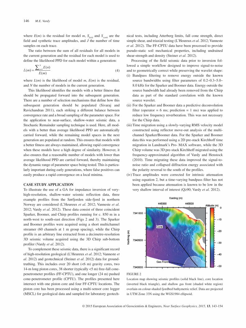
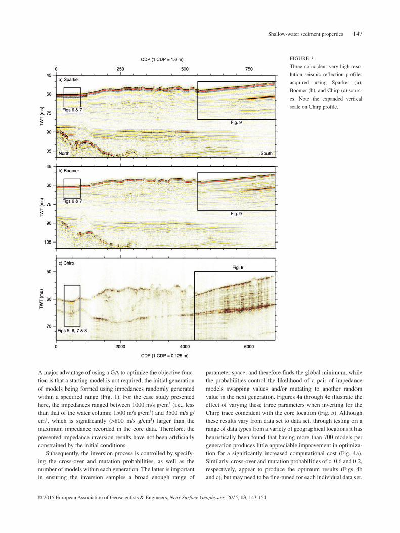
CASE STUDY APPLICATIONTo illustrate the use of a GA for impedance inversion of very-high-resolution, shallow-water seismic reflection data, three example profiles from the Sørfjorden side-fjord in northern Norway are considered (L’Heureux et al. 2012; Vanneste et al. 2012; Vardy et al. 2012). These data consist of three coincident Sparker, Boomer, and Chirp profiles running for c. 850 m in a north-west to south-east direction (Figs 2 and 3). The Sparker and Boomer profiles were acquired using a short multichannel streamer (60 channels at 1 m group spacing), while the Chirp profile is an arbitrary line extracted from a decimetre-resolution 3D seismic volume acquired using the 3D Chirp sub-bottom profiler (Vardy et al. 2012).

To complement these seismic data, there is a significant record of high-resolution geological (L’Heureux et al. 2012; Vanneste et al. 2012) and geotechnical (Steiner et al. 2012) data for ground-truthing. This includes over 20 short (<6 m) gravity cores, two 14-m long piston cores, 38 shorter (typically <5 m) free-fall cone-penetrometer profiles (FF-CPTU), and one longer (24 m) pushed cone-penetrometer profile (CPTU). The profiles presented here intersect with one piston core and four FF-CPTU locations. The piston core has been processed using a multi-sensor core logger (MSCL) for geological data and sampled for laboratory geotech-

FIGURE 2

Location map showing seismic profiles (solid black line), core location

(inverted black triangle), and shallow gas front (shaded white region)

overlain on colour-shaded fjordbed bathymetric relief. Data are projected

in UTM Zone 33N using the WGS1984 ellipsoid.



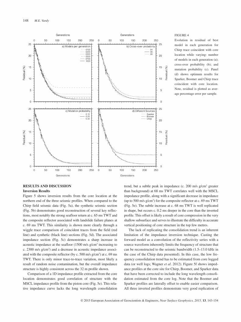
parameter space, and therefore finds the global minimum, while the probabilities control the likelihood of a pair of impedance models swapping values and/or mutating to another random value in the next generation. Figures 4a through 4c illustrate the effect of varying these three parameters when inverting for the Chirp trace coincident with the core location (Fig. 5). Although these results vary from data set to data set, through testing on a range of data types from a variety of geographical locations it has heuristically been found that having more than 700 models per generation produces little appreciable improvement in optimiza-tion for a significantly increased computational cost (Fig. 4a). Similarly, cross-over and mutation probabilities of c. 0.6 and 0.2, respectively, appear to produce the optimum results (Figs 4b and c), but may need to be fine-tuned for each individual data set.

A major advantage of using a GA to optimize the objective func-tion is that a starting model is not required; the initial generation of models being formed using impedances randomly generated within a specified range (Fig. 1). For the case study presented here, the impedances ranged between 1000 m/s g/cm3 (i.e., less than that of the water column; 1500 m/s g/cm3) and 3500 m/s g/cm3, which is significantly (>800 m/s g/cm3) larger than the maximum impedance recorded in the core data. Therefore, the presented impedance inversion results have not been artificially constrained by the initial conditions.

Subsequently, the inversion process is controlled by specify-ing the cross-over and mutation probabilities, as well as the number of models within each generation. The latter is important in ensuring the inversion samples a broad enough range of

FIGURE 3

Three coincident very-high-reso-

lution seismic reflection profiles

acquired using Sparker (a),

Boomer (b), and Chirp (c) sourc-

es. Note the expanded vertical

scale on Chirp profile.

M.E. Vardy148


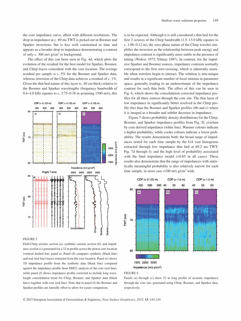
trend, but a subtle peak in impedance (c. 200 m/s g/cm3 greater than background) at 68 ms TWT correlates well with the MSCL impedance profile, along with a significant decrease in impedance (up to 500 m/s g/cm3) for the composite reflector at c. 69 ms TWT (Fig. 5e). The subtle increase at c. 68 ms TWT is well replicated in shape, but occurs c. 0.2 ms deeper in the core than the inverted profile. This offset is likely a result of core compression in the very shallow subsurface and serves to illustrate the difficulty in accurate vertical positioning of core structure in the top few metres.

The lack of replicating the consolidation trend is an inherent limitation of the impedance inversion technique. Casting the forward model as a convolution of the reflectivity series with a source waveform inherently limits the frequency of structure that can be reconstructed to the seismic bandwidth (1.5–13.0 kHz in the case of the Chirp data presented). In this case, the low fre-quency consolidation trend has to be estimated from core logged data (or well logs; Wagner et al. 2012). Figure 5f shows imped-ance profiles at the core site for Chirp, Boomer, and Sparker data that have been corrected to include the long wavelength consoli-dation estimated from the core log. Note that the Boomer and Sparker profiles are laterally offset to enable easier comparison. All three inverted profiles demonstrate very good replication of

RESULTS AND DISCUSSIONInversion ResultsFigure 5 shows inversion results from the core location at the northern end of the three seismic profiles. When compared to the Chirp field seismic data (Fig. 5a), the synthetic seismic section (Fig. 5b) demonstrates good reconstruction of several key reflec-tions, most notably the strong seafloor return at c. 65 ms TWT and the composite reflector associated with landslide failure planes at c. 69 ms TWT. This similarity is shown more clearly through a wiggle trace comparison of coincident traces from the field (red line) and synthetic (black line) sections (Fig. 5d). The associated impedance section (Fig. 5c) demonstrates a sharp increase in acoustic impedance at the seafloor (1500 m/s g/cm3 increasing to c. 2300 m/s g/cm3) and a decrease in acoustic impedance associ-ated with the composite reflector (by c. 500 m/s g/cm3) at c. 69 ms TWT. There is only minor trace-to-trace variation, most likely a result of random noise contamination, but the overall impedance structure is highly consistent across the 32 m profile shown.

Comparison of a 1D impedance profile extracted from the core location demonstrates good correlation of structure with the MSCL impedance profile from the piston core (Fig. 5e). This rela-tive impedance curve lacks the long wavelength consolidation

FIGURE 4

Evolution in residual of best

model in each generation for

Chirp trace coincident with core

location while varying: number

of models in each generation (a);

cross-over probability (b); and

mutation probability (c). Panel

(d) shows optimum results for

Sparker, Boomer and Chirp trace

coincident with core location.

Note, residual is plotted as aver-

age percentage error per sample.



is to be expected. Although it is still considered a thin bed for the first 2 octaves of the Chirp bandwidth (1.5–13.0 kHz equates to c. 1.00–0.12 m), the zero-phase nature of the Chirp wavelet sim-plifies the inversion as the relationship between peak energy and impedance contrast is significantly more stable in the presence of tuning (Widess 1973; Yilmaz 1987). In contrast, for the impul-sive Sparker and Boomer sources, impedance contrasts normally correspond to the first zero-crossing, which is inherently unsta-ble when wavelets begin to interact. The solution is non-unique and results in a significant number of local minima in parameter space, generally leading to an underestimate of the impedance contrast for such thin beds. The effect of this can be seen in Fig. 6, which shows the consolidation corrected impedance pro-files for all three sources through the core site. The thin layer of low impedance in significantly better resolved in the Chirp pro-file (6a) than the Boomer and Sparker profiles (6b and c) where it is imaged as a broader and subtler decrease in impedance.

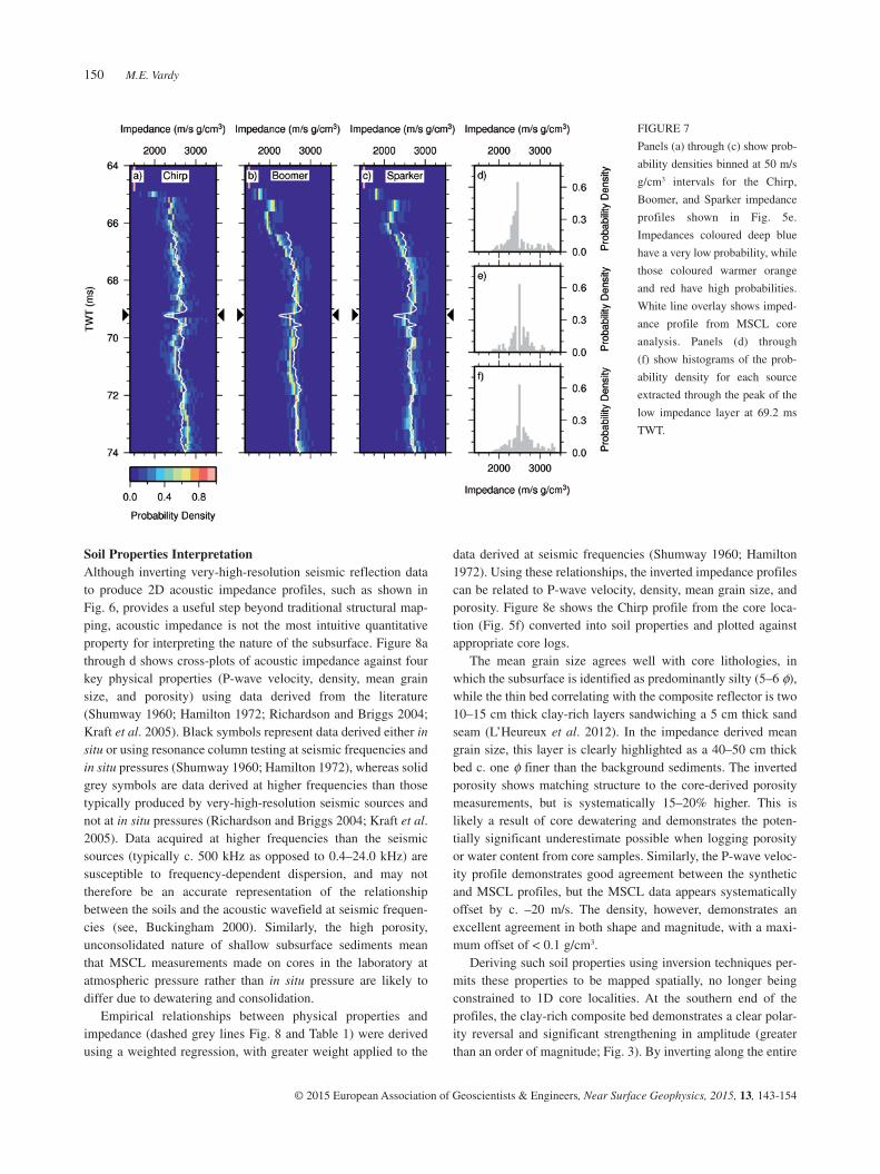
Figure 7 shows probability density distributions for the Chirp, Boomer, and Sparker impedance profiles from Fig. 5f, overlain by core derived impedance (white line). Warmer colours indicate a higher probability, while cooler colours indicate a lower prob-ability. The results demonstrate both: the broad range of imped-ances tested for each time sample by the GA (see histograms extracted through low impedance thin bed at 69.2 ms TWT; Fig. 7d through f); and the high level of probability associated with the final impedance model (>0.65 in all cases). These results also demonstrate that the range of impedances with statis-tically meaningful probability is also relatively narrow for each time sample, in most case <100 m/s g/cm3 wide.

the core impedance curve, albeit with different resolutions. The drop in impedance at c. 69 ms TWT is picked out in Boomer and Sparker inversions, but is less well constrained in time and appears as a broader drop in impedance demonstrating a contrast of only c. 300 m/s g/cm3 to background.

The effect of this can been seen in Fig. 4d, which plots the evolution of the residual for the best model for Sparker, Boomer, and Chirp traces coincident with the core location. The average residual per sample is c. 5% for the Boomer and Sparker data, whereas inversion of the Chirp data achieves a residual of c. 1%. Given the thin bed nature of this layer (c. 40 cm thick) relative to the Boomer and Sparker wavelengths (frequency bandwidth of 0.4–4.0 kHz equates to c. 3.75–0.38 m assuming 1500 m/s), this

FIGURE 5

Field Chirp seismic section (a), synthetic seismic section (b), and imped-

ance section (c) generated for a 32 m profile across the piston core location

(vertical dashed line, panel a). Panel (d) compares synthetic (black line)

and real (red line) traces extracted from the core location. Panel (e) shows

1D impedance profile from the synthetic data (black line) compared

against the impedance profile from MSCL analysis of the core (red line),

while panel (f) shows impedance profile corrected to include long wave-

length consolidation trend for Chirp, Boomer, and Sparker data (black

lines) together with core (red line). Note that in panel (f) the Boomer and

Sparker profiles are laterally offset to allow for easier comparison.

FIGURE 6

Panels (a) through (c) show 32 m long profile of acoustic impedance

through the core site, generated using Chirp, Boomer, and Sparker data,

respectively.

M.E. Vardy150


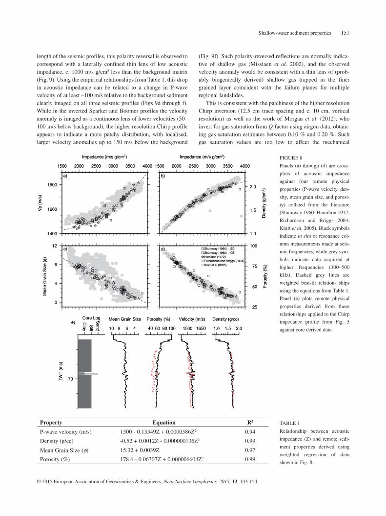
data derived at seismic frequencies (Shumway 1960; Hamilton 1972). Using these relationships, the inverted impedance profiles can be related to P-wave velocity, density, mean grain size, and porosity. Figure 8e shows the Chirp profile from the core loca-tion (Fig. 5f) converted into soil properties and plotted against appropriate core logs.

The mean grain size agrees well with core lithologies, in which the subsurface is identified as predominantly silty (5–6 φ), while the thin bed correlating with the composite reflector is two 10–15 cm thick clay-rich layers sandwiching a 5 cm thick sand seam (L’Heureux et al. 2012). In the impedance derived mean grain size, this layer is clearly highlighted as a 40–50 cm thick bed c. one φ finer than the background sediments. The inverted porosity shows matching structure to the core-derived porosity measurements, but is systematically 15–20% higher. This is likely a result of core dewatering and demonstrates the poten-tially significant underestimate possible when logging porosity or water content from core samples. Similarly, the P-wave veloc-ity profile demonstrates good agreement between the synthetic and MSCL profiles, but the MSCL data appears systematically offset by c. –20 m/s. The density, however, demonstrates an excellent agreement in both shape and magnitude, with a maxi-mum offset of < 0.1 g/cm3.

Deriving such soil properties using inversion techniques per-mits these properties to be mapped spatially, no longer being constrained to 1D core localities. At the southern end of the profiles, the clay-rich composite bed demonstrates a clear polar-ity reversal and significant strengthening in amplitude (greater than an order of magnitude; Fig. 3). By inverting along the entire

Soil Properties InterpretationAlthough inverting very-high-resolution seismic reflection data to produce 2D acoustic impedance profiles, such as shown in Fig. 6, provides a useful step beyond traditional structural map-ping, acoustic impedance is not the most intuitive quantitative property for interpreting the nature of the subsurface. Figure 8a through d shows cross-plots of acoustic impedance against four key physical properties (P-wave velocity, density, mean grain size, and porosity) using data derived from the literature (Shumway 1960; Hamilton 1972; Richardson and Briggs 2004; Kraft et al. 2005). Black symbols represent data derived either in situ or using resonance column testing at seismic frequencies and in situ pressures (Shumway 1960; Hamilton 1972), whereas solid grey symbols are data derived at higher frequencies than those typically produced by very-high-resolution seismic sources and not at in situ pressures (Richardson and Briggs 2004; Kraft et al. 2005). Data acquired at higher frequencies than the seismic sources (typically c. 500 kHz as opposed to 0.4–24.0 kHz) are susceptible to frequency-dependent dispersion, and may not therefore be an accurate representation of the relationship between the soils and the acoustic wavefield at seismic frequen-cies (see, Buckingham 2000). Similarly, the high porosity, unconsolidated nature of shallow subsurface sediments mean that MSCL measurements made on cores in the laboratory at atmospheric pressure rather than in situ pressure are likely to differ due to dewatering and consolidation.

Empirical relationships between physical properties and impedance (dashed grey lines Fig. 8 and Table 1) were derived using a weighted regression, with greater weight applied to the

FIGURE 7

Panels (a) through (c) show prob-

ability densities binned at 50 m/s

g/cm3 intervals for the Chirp,

Boomer, and Sparker impedance

profiles shown in Fig. 5e.

Impedances coloured deep blue

have a very low probability, while

those coloured warmer orange

and red have high probabilities.

White line overlay shows imped-

ance profile from MSCL core

analysis. Panels (d) through

(f) show histograms of the prob-

ability density for each source

extracted through the peak of the

low impedance layer at 69.2 ms

TWT.



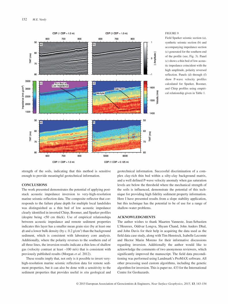
(Fig. 9f). Such polarity-reversed reflections are normally indica-tive of shallow gas (Missiaen et al. 2002), and the observed velocity anomaly would be consistent with a thin lens of (prob-ably biogenically derived) shallow gas trapped in the finer grained layer coincident with the failure planes for multiple regional landslides.

This is consistent with the patchiness of the higher resolution Chirp inversion (12.5 cm trace spacing and c. 10 cm, vertical resolution) as well as the work of Morgan et al. (2012), who invert for gas saturation from Q-factor using airgun data, obtain-ing gas saturation estimates between 0.10 % and 0.20 %. Such gas saturation values are too low to affect the mechanical

length of the seismic profiles, this polarity reversal is observed to correspond with a laterally confined thin lens of low acoustic impedance, c. 1000 m/s g/cm3 less than the background matrix (Fig. 9). Using the empirical relationships from Table 1, this drop in acoustic impedance can be related to a change in P-wave velocity of at least –100 m/s relative to the background sediment clearly imaged on all three seismic profiles (Figs 9d through f). While in the inverted Sparker and Boomer profiles the velocity anomaly is imaged as a continuous lens of lower velocities (50–100 m/s below background), the higher resolution Chirp profile appears to indicate a more patchy distribution, with localised, larger velocity anomalies up to 150 m/s below the background

FIGURE 8

Panels (a) through (d) are cross-

plots of acoustic impedance

against four remote physical

properties (P-wave velocity, den-

sity, mean grain size, and porosi-

ty) collated from the literature

(Shumway 1960; Hamilton 1972;

Richardson and Briggs 2004;

Kraft et al. 2005). Black symbols

indicate in situ or resonance col-

umn measurements made at seis-

mic frequencies, while grey sym-

bols indicate data acquired at

higher frequencies (300–500

kHz). Dashed grey lines are

weighted best-fit relationships

using the equations from Table 1.

Panel (e) plots remote physical

properties derived from these

relationships applied to the Chirp

impedance profile from Fig. 5

against core derived data.

Property Equation R2

P-wave velocity (m/s) 1500 - 0.13549Z + 0.0000586Z2 0.94

Density (g/cc) -0.52 + 0.0012Z - 0.000000136Z2 0.99

Mean Grain Size (φ) 15.32 + 0.0039Z 0.97

Porosity (%) 178.6 - 0.06307Z + 0.000006604Z2 0.99

TABLE 1

Relationship between acoustic

impedance (Z) and remote sedi-

ment properties derived using

weighted regression of data

shown in Fig. 8.

M.E. Vardy152


geotechnical information. Successful discrimination of a com-plex clay-rich thin bed within a silty-clay background matrix, and a well defined P-wave velocity anomaly when gas saturation levels are below the threshold where the mechanical strength of the soils is influenced, demonstrate the potential of this tech-nique for providing high fidelity sediment property information. Here I have presented results from a slope stability application, but this technique has the potential to be of use for a range of shallow-water problems.

ACKNOWLEDGMENTSThe author wishes to thank Maarten Vanneste, Jean-Sebastien L’Heureux, Oddvar Longva, Shyam Chand, John Anders Dhal, and John Davis for their help in acquiring the data used as the field data case study, along with Tim Henstock, Isabelle Lecomte and Hector Marin Moreno for their informative discussions regarding inversion. Additionally the author would like to acknowledge the comments of two anonymous reviewers, which significantly improved the manuscript. The field data precondi-tioning was performed using Landmark’s ProMAX software. All other processing used custom algorithms, including the genetic algorithm for inversion. This is paper no. 433 for the International Centre for Geohazards.

strength of the soils, indicating that this method is sensitive enough to provide meaningful geotechnical information.

CONCLUSIONSThe work presented demonstrates the potential of applying post-stack acoustic impedance inversion to very-high-resolution marine seismic reflection data. The composite reflector that cor-responds to the failure plane depth for multiple local landslides was distinguished as a thin bed of low acoustic impedance clearly identified in inverted Chirp, Boomer, and Sparker profiles (despite being <50 cm thick). Use of empirical relationships between acoustic impedance and remote sediment properties indicates this layer has a smaller mean grain size (by at least one φ) and a lower bulk density (by c. 0.2 g/cm3) than the background sediment, which is consistent with laboratory core analysis. Additionally, where the polarity reverses to the southern end of all three lines, the inversion results indicate a thin lens of shallow gas (velocity contrast at least –100 m/s) that is consistent with previously published results (Morgan et al. 2012).

These results imply that, not only is it possible to invert very-high-resolution marine seismic reflection data for remote sedi-ment properties, but it can also be done with a sensitivity to the sediment properties that provides useful in situ geological and

FIGURE 9

Field Sparker seismic section (a),

synthetic seismic section (b) and

accompanying impedance section

(c) generated for the southern end

of the profile (see, Fig. 3). Panel

(c) shows a thin bed of low acous-

tic impedance coincident with the

high amplitude, polarity reversed

reflection. Panels (d) through (f)

show P-wave velocity profiles

calculated for Sparker, Boomer,

and Chirp profiles using empiri-

cal relationship given in Table 1.



Muller C., Woelz S., Ersoy Y., Boyce J., Jokisch T., Wendt G. and Rabbel W. 2009. Ultra-high-resolution marine 2D-3D seismic inves-tigation of the Liman Tepe/Karatina Island archaeological site (Urla/Turkey). Journal of Applied Geophysics 68, 124–134.

Oldenburg D., Scheuer T. and Levy S. 1983. Recovery of the acoustic impedance from reection seismograms. Geophysics 48, 1318–1337.

Palamenghi L., Schwenk T., Spiess V. and Kudrass H. 2011. Seismostratigraphic analysis with centennial to decadal time resolu-tion of the sediment sink in the Ganges–Brahmaputra subaqueous delta. Continental Shelf Research 31(6), 712–730.

Panda S., LeBlanc L. and Schock S. 1994. Sediment classi_cation based on impedance and attenuation estimation. J. Acoustic. Soc. Amer. 96(5), 3022–3035.

Pinson L., Henstock T., Dix J. and Bull J. 2008. Estimating quality fac-tor and mean grain size of sediments from high-resolution marine seismic data. Geophysics 73(4), G19–G28.

Pinson L., Vardy M., Dix J., Henstock T., Bull J. and MacLachlan S. 2013. Deglacial history of glacial lake Windermere, UK; implications for the central British and Irish Ice Sheet. Journal of Quaternary Science 28(1), 83–94.

Plets R., Dix J., Adams J. and Best A. 2008. 3D Reconstruction of a Shallow Archaeological Site from High-Resolution Acoustic Imagery: the Grace Dieu. Applied Acoustics 69, 399–411.

Richardson M. and Briggs K. 2004. Empirical Predictions of Seafloor Properties Based on Remotely Measured Sediment Impedance. In: High Frequency Ocean Acoustics Conference, pp. 12–21, AIP, Melville, NY.

Schock S., LeBlanc L. and Mayer L. 1989. Chirp subottom profiler for quantitative sediment analysis. Geophysics 54(4), 445–450.

Schock S., Tellier A., Wulf J., Sara J. and Ericksen M. 2001. Buried object scanning sonar. IEEE Journal of Ocean Engineering 26(4), 677–689.

Sen M. and Stoffa P. 1991. Nonlinear one dimensional seismic wave-form inversion using simulated annealing. Geophysics 56(10), 1624–1638.

Sen M. and Stoffa P. 1992. Rapid sampling of model space using genetic algorithms: Examples from seismic waveform inversion. Geophysical Journal International 108, 281–292.

Sen M. and Stoffa P. 1996. Bayesian inference, Gibb’s sampler and uncertainty estimation in geophysical inversion. Geophysical Prospecting 44, 313–350.

Sheriff R. 2002. Encyclopedic Dictionary of Applied Geophysics. In: Geophysical Reference Series 13, SEG, 4th edn.

Shumway G. 1960. Sound speed and absorption studies of marine sedi-ments by a resonance method. Geophysics 25(2), 451–467.

Sivaraj R. and Ravichandran T. 2011. A review of selection methods in Genetic Algorithms. International Journal of Engineering Science and Technology 3(5), 3792–3797.

Steiner A., L’Heureux J.-S., Kopf A., Vanneste M., Longva O., Lange M. et al. 2012. An In-Situ Free-Fall Piezocone Penetrometer for Characterizing Soft and Sensitive Clays at Finneidfjord (Northern Norway). In: Submarine Mass Movements and Their Consequences, vol. 31 of Advances in Natural and Technological Hazards Research, pp. 99–109, Springer, Heidelberg, DE.

Stevenson I., McCann C. and Runciman P. 2002. An attenuation-based sediment classification technique using Chirp sub-bottom profiler data and laboratory acoustic analysis. Marine Geophysical Researches 23, 277–298.

Stoffa P. and Sen M. 1991. Nonlinear multiparameter optimization using genetic algorithms: inversion of plane wave seismograms. Geophysics 56(11), 1794–1810.

Stoker M., Bradwell T., Howe J., Wilkinson I. and McIntyre K. 2009. Lateglacial ice-cap dynamics in NW Scotland: evidence from the

REFERENCESBiondi B. 2007. Concepts and Applications in 3D Seismic Imaging. In:

SEG Distinguished Instructor Short Course 10, SEG, Tulsa, Oklahoma, USA.

Bleistein N. 2001. Mathematics of Multidimensional Seismic Imaging, Migration, and Inversion. Springer-Verlag, Inc.

Bosch M., Mukerji T. and Gonzalez E. 2010. Seismic inversion for reservoir properties combining statistical rock physics and geostatis-tics: a review. Geophysics 75, A165–A176.

Buckingham M. 2000. Wave propagation, stress relaxation, and grain-to-grain shearing in saturated, unconsolidated marine sediments. Journal of the Acoustics Society of America 108, 2796–2815.

Bull J.M., Quinn R. and Dix J. 1998. Reflection coefficient calculation from marine high-resolution seismic reflection (Chirp) data and application to an archaeological case study. Marine Geophysical Researches 20, 1–11.

Cooke D.A. and Schneider W.A. 1983. Generalized linear inversion of reflection seismic data. Geophysics, 48(6), 665–676.

Edgar J. And van der Baan M. 2011. How reliable is statistical wavelet estimation? Geophysics 76(4), V59–V68.

Goldberg D. 1989. Genetic Algorithms in Search, Optimization, and Machine Learning, Addison Wesley Publishing Company, Reading, MA.

Gutowski M., Bull J.M., Dix J., Henstock T., Hogarth P., White P. and Leighton T. 2002. Chirp sub-bottom profiler source signature design and field testing. Marine Geophysical Researches 23, 481–492.

Gutowski M., Bull J.M., Dix J., Henstock T.J., Hogarth P., Hiller T., Leighton T. and White P. 2008. 3D high-resolution acoustic imaging of the sub-seabed. Applied Acoustics 69(5), 412–421.

Hamilton E. 1972. Compressional Wave Attenuation in Marine Sediments. Geophysics 37(4), 620–646.

Kraft B., Ressler J., Mayer L., Fonseca L. and McGillicuddy G. 2005. In-situ measurement of sediment acoustic properties. In: Proceedings of the International Conference Underwater Acoustic Measurements: Technologies and Results, Acoustical Society of America.

L’Heureux J.-S., Longva O., Steiner A., Hansen L., Vardy M., Vanneste M. et al. 2012. Identification of Weak Layers and Their Role for the Stability of Slopes at Finneidfjord, Northern Norway. In: Submarine Mass Movements and Their Consequences 31, Advances in Natural and Technological Hazards Research, pp. 321–330, Springer, Heidelberg, DE.

Mallick S. 2001. Prestack waveform inversion using a genetic algorithm – The present and the future. CSEG Recorder 26(6), 78–84.

Missiaen T., Murphy S., Loncke L. and Henriet J.-P. 2002. Very high-resolution seismic mapping of shallow gas in the Belgian coastal zone. Continental Shelf Research 22, 2291–2301.

Morgan E., Vanneste M., Lecomte I., Baise L., Longva O. and McAdoo B. 2012. Estimation of free gas saturation from seismic reflection surveys by the genetic algorithm inversion of a P-wave attenuation model. Geophysics 77(4), R175–R187.

Morgan J., Warner M., Collins G., Grieve R., Christeson G., Gulick S. et al. 2011. Full waveform tomographic images of the peak ring at the Chicxulub impact crater. Journal of Geophysical Research 116, B06303.

Morgan J., Warner M., Bell R., Ashley J., Barnes D., Little R., Roele K. and Jones C. 2013. Next-generation seismic experiments: wide-angle, multi-azimuth, three-dimensional, full-waveform inversion. Geophysical Journal International 195, 1657–1678.

Mueller C., Woelz S. and Kalmring S. 2013. High-Resolution 3D Marine Seismic Investigation of Hedeby Harbour, Germany. The International Journal of Nautical Archaeology 42(2), 326–336.

Muller C., Mikereit B., Bohlen T. and Theilen F. 2002. Towards high-resolution 3D marine seismic surveying using Boomer sources. Geophysical Prospecting 50, 517–526.

M.E. Vardy154


Vardy M., L’Heureux J.-S., Vanneste M., Longva O., Steiner A., Forsberg C. et al. 2012. Multidisciplinary investigation of a shallow near-shore landslide, Finneidfjord, Norway. Near Surface Geophysics 10, 267–277.

Verbeek N. and McGee T. 1995. Characteristics of high-resolution marine reflection profiling sources. Journal of Applied Geophysics 33, 251–269.

Wagner C., Gonzalez A., Agarwal V., Koesoemadinata A., Ng D., Trares S., Biles N. and Fisher K. 2012. Quantitative application of poststack acoustic impedance inversion to subsalt reservoir development. The Leading Edge 31, 528–537.

Wardell N., Diviacco P. and Sinceri R. 2002. 3D pre-processing tech-niques for marine VHR seismic data. First Break 20(7).

Widess M.B. 1973. How Thin is a Thin Bed? Geophysics 6, 1176–1180.Yilmaz O. 1987. Seismic Data Processing, vol. 2 of Investigations in

Geophysics, SEG, Tulsa, USA, 1st ed.

fjords of the Summer Isles region. Quaternary Science Reviews 28, 3161–3184.

Vanneste M., L’Heureux J.-S., Brendryen J., Baeten N., Larberg J., Vardy M. et al. 2012. Assessing offshore geohazards: A multi-disci-plinary research initiative to understand shallow landslides and their dynamics in coastal and deepwater environments, Norway. In: Submarine Mass Movements and Their Consequences, vol. 31 of Advances in Natural and Technological Hazards Research, pp. 29–41, Springer, Heidelberg, DE.

Vardy M. and Henstock T. 2010. A frequency approximated approach to Kirchho_ migration. Geophysics 75(6), S211–S218.

Vardy M., Dix J., Henstock T., Bull J. and Gutowski M. 2008. Decimetre-resolution 3D seismic volume in shallow water; a case study in small object detection. Geophysics 73(2), B33–B40.

Vardy M., Pinson L., Bull J., Dix J., Henstock T., Davis J. and Gutowski M. 2010. 3D seismic imaging of buried Younger Dryas mass move-ment flows: Lake Windermere, UK. Geomorphology 118, 176–187.

Geophysical Equipment Source FOR SALES AND RENTALS

www.geomatrix.co.uk

Our expertise covers mineral exploration, all types of near surface surveys, marine geophysics, UXO and surveys for other manmade hazards

T: +44 (0)1525 383438E: [email protected]

20 Eden Way, Pages Industrial Park, Leighton Buzzard, Beds LU7 4TZ. UK.

CC02532-MA003 Geomatrix.indd 1 08-01-15 16:51

Documents

Deriving shallow-water sediment properties using post ...mev/pubs/Vardy-2015.pdf · Deriving shallow-water sediment properties using ... Edgar and van der Baan 2011). However,