sensors

Article

Curve-Based Classification Approach for HyperspectralDermatologic Data Processing

Stig Uteng 1,* , Eduardo Quevedo 2 , Gustavo M. Callico 2 , Irene Castaño 3, Gregorio Carretero 3,Pablo Almeida 4, Aday Garcia 5 , Javier A. Hernandez 4 and Fred Godtliebsen 6

�����������������

Citation: Uteng, S.; Quevedo, E.; M.

Callico, G.; Castaño, I.; Carretero, G.;

Almeida, P.; Garcia, A.; A. Hernandez,

J.; Godtliebsen, F. Curve-Based

Classification Approach for

Hyperspectral Dermatologic Data

Processing. Sensors 2021, 21, 680.

https://doi.org/10.3390/s21030680

Received: 15 December 2020

Accepted: 15 January 2021

Published: 20 January 2021

Publisher’s Note: MDPI stays neutral

with regard to jurisdictional claims in

published maps and institutional affil-

iations.

Copyright: © 2021 by the authors.

Licensee MDPI, Basel, Switzerland.

This article is an open access article

distributed under the terms and

conditions of the Creative Commons

Attribution (CC BY) license (https://

creativecommons.org/licenses/by/

4.0/).

1 Department of Education and Pedagogy, UiT the Arctic University of Norway, 9019 Tromsø, Norway2 Institute for Applied Microelectronics, Universidad de Las Palmas de Gran Canaria,

35016 Las Palmas de Gran Canaria, Spain; eduardo.quevedo@ulpgc.es (E.Q.);gustavo@iuma.ulpgc.es (G.M.C.)

3 Department of Dermatology, Hospital Universitario de Gran Canaria Doctor Negrín,35016 Las Palmas de Gran Canaria, Spain; irenecastano@hotmail.com (I.C.);gcarher@gobiernodecanarias.org (G.C.)

4 Department of Dermatology, Complejo Hospitalario Universitario Insular-Materno Infantil,35016 Las Palmas de Gran Canaria, Spain; pjalmmar75@gmail.com (P.A.);jhersant@gobiernodecanarias.org (J.A.H.)

5 Department of Electromedicine, Complejo Hospitalario Universitario Insular-Materno Infantil,35016 Las Palmas de Gran Canaria, Spain; agarcia@iuma.ulpgc.es

6 Department of Mathematics and Statistics, UiT the Arctic University of Norway, 9019 Tromsø, Norway;fred.godtliebsen@uit.no

* Correspondence: stig.uteng@uit.no

Abstract: This paper shows new contributions in the detection of skin cancer, where we presentthe use of a customized hyperspectral system that captures images in the spectral range from 450to 950 nm. By choosing a 7 × 7 sub-image of each channel in the hyperspectral image (HSI) andthen taking the mean and standard deviation of these sub-images, we were able to make fits of theresulting curves. These fitted curves had certain characteristics, which then served as a basis ofclassification. The most distinct fit was for the melanoma pigmented skin lesions (PSLs), which isalso the most aggressive malignant cancer. Furthermore, we were able to classify the other PSLs inmalignant and benign classes. This gives us a rather complete classification method for PSLs witha novel perspective of the classification procedure by exploiting the variability of each channel inthe HSI.

Keywords: hyperspectral; curve fit; statistical discrimination; melanoma; benign; malignant

1. Introduction

Hyperspectral (HS) imaging (HSI) combines conventional imaging and spectroscopymethods in a single imaging technique providing both spatial and spectral informationof the captured display [1,2]. It is also a fitting method for medical applications due to itsnon-invasive, non-ionizing, and label-free nature [3]. Dermatology is one of the medicalfields where HSI have shown its potential as an appropriate imaging technique [4].

Currently, the most common form of cancer, with more than 1.3 million new casesworldwide in 2018, is skin cancer [5]. There are several types of skin lesions. Pigmentedskin lesions (PSLs) contain a wide variety of types, including cancerous and non-cancerousPSLs [6]. There are two types of PSLs depending on the type of growth of the tissue: benignand malignant. Nevus, which is benign, has a slow growth rate and is noncancerous, whilee.g., melanomas, which is malignant, are invasive and potentially metastatic tumors [6].Other types of skin cancer produced by different types of cells include squamous cellcarcinoma and basal cell carcinoma. However, melanomas are much more dangerousthan other types of skin cancer, and an early detection of this skin lesion can be extremely

Sensors 2021, 21, 680. https://doi.org/10.3390/s21030680 https://www.mdpi.com/journal/sensors

Sensors 2021, 21, 680 2 of 13

important in improving the patient survival [7]. The diagnosis of PSLs is performed bydermatologists employing their naked eye or dermascopic cameras, which enhance themorphological visualization of the PSL. After the inspection, an analysis of the lesionfollowing the ABCDE (Asymmetry, Border irregularity, Color, Diameter and Evolvingsize, shape, or color) rule is applied in order to establish a preliminary diagnosis [7]. Asuspicious lesion will accordingly get a histopathological analysis carried out to determinethe definitive diagnosis. These diagnostic tools based on conventional imaging have beenused to help dermatologists in preliminary diagnosis. However, conventional imaging haslimitations that could be surpassed by the enriched spectral information provided by theHSIs.

HSI technology has already been explored as a target technology to aid in PSLs diagno-sis. A recent study by Leon et al. showed promising results in discriminating PSLs by ran-dom forests and artificial neural networks [8]. Another recent study by Hosking et al. useddigital dermascopy HSI with machine learning methods in order to detect melanomas [9].Kazianka et al. used HSIs to differentiate between normal skin, melanomas, and moles [10].They used unsupervised approaches to segment the images and moreover evaluated theperformance of several supervised classifiers aimed to retrieve the diagnosis of each pixel.The results indicated that it was possible to differentiate melanomas from moles withhigh specificity and sensitivity. In another study, Nagaoka et al. [11] collected a datasetfor discriminating between melanomas and other PSLs, evaluating the statistical signifi-cance of an index defined to this end. Tomatis et al. used a classifier based on a neuralnetwork model [12]. There have also been developed some commercial systems as SIAs-cope/SIAscopy [13] and MelaFind [14–16]. MelaFind is being used in several studies.In [15], Elbaum et al. conduct a leave-one-out cross-validation procedure using a databasecomposed of 183 melanocytic nevus and 63 melanomas. Monheit et al. [16] applied it in amulticenter study. At last, Song et al. performed a paired comparison between MelaFindand a reflectance confocal microscopy system to differentiate between melanoma andnon-melanoma PSLs by comparing MelaFind with a confocal microscopy system. In thestudy by Stamnes et al., they discriminate between malignant and benign PSLs, i.e., nospecific melanoma detection [17].

The current default method of data analysis (DA) is deep learning (DL). DL emergedas a competing DA method around 2009 and solves a wide range of problems exemplifiedby the versatile TensorFlow-package [18]. DL is also applied in the HSI field. However, DLoften needs a huge amount of data in order to train the parameters enough in the neuralnetwork [19]. Thus, in the proposed method, this presents a difficult problem due to thelack of data. We are pursuing this problem by an ongoing data collection project, aimingfor future applications of DL systems.

Most of the research in the use of HSI for skin analysis is focused on the automaticdiagnosis of PSLs. Clearly, a successful methodology of this type would be an extremelyuseful decision support tool for general practitioners (GPs) and dermatologists. In ourcontribution in this direction, we were able to find clear patterns for the melanoma PSLs,the other malignant PSLs and the benign PSLs. In the novel exploitation of the variabilityof each channel in the HSI cubes, we made curves of the mean and standard deviation ofsub-images in these channels. Furthermore, using these curves and their inherent patterns,we were able to discriminate between malignant and benign PSLs, but also between theaggressive melanoma PSL and the others.

The outline of the paper is as follows. First, we describe the developed dermatologicalHSI acquisition system, and thereafter, we describe the datasets we are using in this curve-based classification method. Next, we point out how the data are pre-processed and labeledbefore they are used as input in our new classification method, which consists of a training,validation, and testing phase.

Sensors 2021, 21, 680 3 of 13

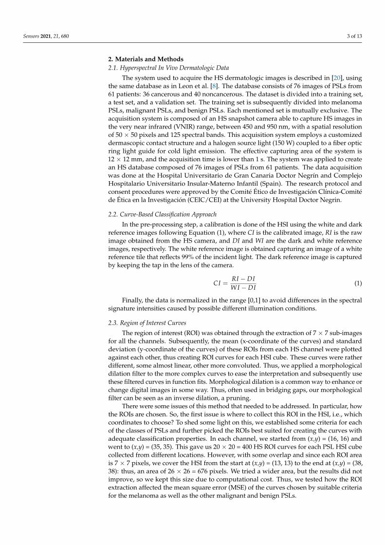
2. Materials and Methods2.1. Hyperspectral In Vivo Dermatologic Data

The system used to acquire the HS dermatologic images is described in [20], usingthe same database as in Leon et al. [8]. The database consists of 76 images of PSLs from61 patients: 36 cancerous and 40 noncancerous. The dataset is divided into a training set,a test set, and a validation set. The training set is subsequently divided into melanomaPSLs, malignant PSLs, and benign PSLs. Each mentioned set is mutually exclusive. Theacquisition system is composed of an HS snapshot camera able to capture HS images inthe very near infrared (VNIR) range, between 450 and 950 nm, with a spatial resolutionof 50 × 50 pixels and 125 spectral bands. This acquisition system employs a customizeddermascopic contact structure and a halogen source light (150 W) coupled to a fiber opticring light guide for cold light emission. The effective capturing area of the system is12 × 12 mm, and the acquisition time is lower than 1 s. The system was applied to createan HS database composed of 76 images of PSLs from 61 patients. The data acquisitionwas done at the Hospital Universitario de Gran Canaria Doctor Negrín and ComplejoHospitalario Universitario Insular-Materno Infantil (Spain). The research protocol andconsent procedures were approved by the Comité Ético de Investigación Clínica-Comitéde Ética en la Investigación (CEIC/CEI) at the University Hospital Doctor Negrin.

2.2. Curve-Based Classification Approach

In the pre-processing step, a calibration is done of the HSI using the white and darkreference images following Equation (1), where CI is the calibrated image, RI is the rawimage obtained from the HS camera, and DI and WI are the dark and white referenceimages, respectively. The white reference image is obtained capturing an image of a whitereference tile that reflects 99% of the incident light. The dark reference image is capturedby keeping the tap in the lens of the camera.

CI =RI − DIWI − DI

(1)

Finally, the data is normalized in the range [0,1] to avoid differences in the spectralsignature intensities caused by possible different illumination conditions.

2.3. Region of Interest Curves

The region of interest (ROI) was obtained through the extraction of 7 × 7 sub-imagesfor all the channels. Subsequently, the mean (x-coordinate of the curves) and standarddeviation (y-coordinate of the curves) of these ROIs from each HS channel were plottedagainst each other, thus creating ROI curves for each HSI cube. These curves were ratherdifferent, some almost linear, other more convoluted. Thus, we applied a morphologicaldilation filter to the more complex curves to ease the interpretation and subsequently usethese filtered curves in function fits. Morphological dilation is a common way to enhance orchange digital images in some way. Thus, often used in bridging gaps, our morphologicalfilter can be seen as an inverse dilation, a pruning.

There were some issues of this method that needed to be addressed. In particular, howthe ROIs are chosen. So, the first issue is where to collect this ROI in the HSI, i.e., whichcoordinates to choose? To shed some light on this, we established some criteria for eachof the classes of PSLs and further picked the ROIs best suited for creating the curves withadequate classification properties. In each channel, we started from (x,y) = (16, 16) andwent to (x,y) = (35, 35). This gave us 20 × 20 = 400 HS ROI curves for each PSL HSI cubecollected from different locations. However, with some overlap and since each ROI areais 7 × 7 pixels, we cover the HSI from the start at (x,y) = (13, 13) to the end at (x,y) = (38,38): thus, an area of 26 × 26 = 676 pixels. We tried a wider area, but the results did notimprove, so we kept this size due to computational cost. Thus, we tested how the ROIextraction affected the mean square error (MSE) of the curves chosen by suitable criteriafor the melanoma as well as the other malignant and benign PSLs.

Sensors 2021, 21, 680 4 of 13

The CPU used to run the code was an Intel Xeon 2.8 GHz running on a 16 GB RAMcomputer.

Curve-Fitting

By trying to classify the PSLs through fits of the ROI curves, all the HSI ROI curveswere fitted by a quartic (fourth degree) polynomial function, where the coefficients arefound through the nlinfit function of MATLAB®, which minimizes the weighted leastsquares equation,

∑ni=1 wi(yi − f (xi, b))2 (2)

where the weights were chosen through a weight function, w(y) = 1/(0.011 + 0.011y)2 andn = 125, the number of data points. Further is f (x, b) = b0 x4 + b1 x3 + b2 x2 + b3 x + b4,the quartic regression function, with parameters bj, j = 0, . . . ,4. Then, the nlinfit-functionuses the iteratively reweighted least-square algorithm, which is designed to deal withoutliers [21]. Furthermore, the use of a quartic polynomial with a weight function provedto be the best option with regard to flexibility and robustness to outliers. We also testedhigher degree polynomial functions; however, they were prone to overfitting.

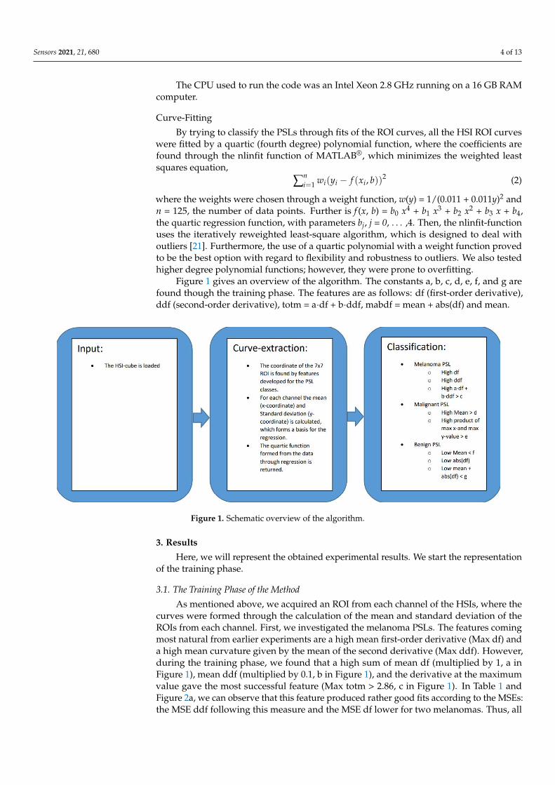
Figure 1 gives an overview of the algorithm. The constants a, b, c, d, e, f, and g arefound though the training phase. The features are as follows: df (first-order derivative),ddf (second-order derivative), totm = a·df + b·ddf, mabdf = mean + abs(df) and mean.

Sensors 2021, 21, x FOR PEER REVIEW  4 of 13  

 

extraction affected the mean square error (MSE) of the curves chosen by suitable criteria 

for the melanoma as well as the other malignant and benign PSLs. 

The CPU used to run the code was an Intel Xeon 2.8 GHz running on a 16 GB RAM 

computer. 

Curve‐Fitting 

By trying to classify the PSLs through fits of the ROI curves, all the HSI ROI curves 

were fitted by a quartic (fourth degree) polynomial function, where the coefficients are 

found  through  the nlinfit  function of MATLAB®, which minimizes  the weighted  least 

squares equation, 

𝑤 𝑦 𝑓 𝑥 , 𝑏   (2) 

where the weights were chosen through a weight function, w(y) = 1/(0.011 + 0.011y)2 and 

n = 125, the number of data points. Further is f(x, b) = b0 x4 + b1 x3 + b2 x2 + b3 x + b4, the quartic 

regression function, with parameters bj, j = 0,…,4. Then, the nlinfit‐function uses the iter‐

atively reweighted  least‐square algorithm, which  is designed to deal with outliers [21]. 

Furthermore, the use of a quartic polynomial with a weight function proved to be the best 

option with regard to flexibility and robustness to outliers. We also tested higher degree 

polynomial functions; however, they were prone to overfitting. 

Figure 1 gives an overview of the algorithm. The constants a, b, c, d, e, f, and g are 

found though the training phase. The features are as follows: df (first‐order derivative), 

ddf (second‐order derivative), totm = a∙df + b∙ddf, mabdf = mean + abs(df) and mean. 

 

Figure 1. Schematic overview of the algorithm. 

3. Results 

Here, we will represent the obtained experimental results. We start the representa‐

tion of the training phase. 

3.1. The Training Phase of the Method 

As mentioned above, we acquired an ROI from each channel of the HSIs, where the 

curves were formed through the calculation of the mean and standard deviation of the 

ROIs from each channel. First, we investigated the melanoma PSLs. The features coming 

most natural from earlier experiments are a high mean first‐order derivative (Max df) and 

a high mean curvature given by the mean of the second derivative (Max ddf). However, 

during the training phase, we found that a high sum of mean df (multiplied by 1, a  in 

Figure 1. Schematic overview of the algorithm.

3. Results

Here, we will represent the obtained experimental results. We start the representationof the training phase.

3.1. The Training Phase of the Method

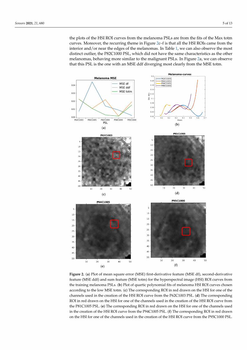
As mentioned above, we acquired an ROI from each channel of the HSIs, where thecurves were formed through the calculation of the mean and standard deviation of theROIs from each channel. First, we investigated the melanoma PSLs. The features comingmost natural from earlier experiments are a high mean first-order derivative (Max df) anda high mean curvature given by the mean of the second derivative (Max ddf). However,during the training phase, we found that a high sum of mean df (multiplied by 1, a inFigure 1), mean ddf (multiplied by 0.1, b in Figure 1), and the derivative at the maximumvalue gave the most successful feature (Max totm > 2.86, c in Figure 1). In Table 1 andFigure 2a, we can observe that this feature produced rather good fits according to the MSEs:the MSE ddf following this measure and the MSE df lower for two melanomas. Thus, all

Sensors 2021, 21, 680 5 of 13

the plots of the HSI ROI curves from the melanoma PSLs are from the fits of the Max totmcurves. Moreover, the recurring theme in Figure 2c–f is that all the HSI ROIs came from theinterior and/or near the edges of the melanomas. In Table 1, we can also observe the mostdistinct outlier, the P82C1000 PSL, which did not have the same characteristics as the othermelanomas, behaving more similar to the malignant PSLs. In Figure 2a, we can observethat this PSL is the one with an MSE ddf diverging most clearly from the MSE totm.

Sensors 2021, 21, x FOR PEER REVIEW  5 of 13  

 

Figure 1), mean ddf (multiplied by 0.1, b in Figure 1), and the derivative at the maximum 

value gave the most successful feature (Max totm > 2.86, c  in Figure 1). In Table 1 and 

Figure 2a, we can observe  that  this  feature produced  rather good  fits according  to  the 

MSEs:  the MSE ddf following  this measure and  the MSE df  lower for  two melanomas. 

Thus, all the plots of the HSI ROI curves from the melanoma PSLs are from the fits of the 

Max totm curves. Moreover, the recurring theme in Figure 2c–f is that all the HSI ROIs 

came from the interior and/or near the edges of the melanomas. In Table 1, we can also 

observe the most distinct outlier, the P82C1000 PSL, which did not have the same charac‐

teristics as the other melanomas, behaving more similar to the malignant PSLs. In Figure 

2a, we can observe that this PSL is the one with an MSE ddf diverging most clearly from 

the MSE totm. 

Table 1. The results for the region of interest (ROI) investigation for the melanoma pigmented skin 

lesions (PSLs) with the corresponding curves with maximum mean first derivative, Max df, maxi‐

mum curvature, Max ddf, maximum weighted sum of mean df, mean ddf and df at the maximum 

point, Max totm and the corresponding MSEs of the chosen curves. 

PSL  Max df  Max ddf  Max totm  MSE df  MSE ddf  MSE totm 

P62C1003  0.19959  5.2261  1.2716  0.00729  0.022353  0.022353 

P81C1005  0.90111  14.465  5.0123  0.044138  0.010691  0.010691 

P82C1000  0.17383  –0.1158  −0.3373  0.01381  0.021781  0.0026241 

P94C1005  1.1388  45.812  5.0485  0.008742  0.001214  0.0012136 

P95C1000  0.60491  19.092  3.3212  0.001983  0.019006  0.015033 

 

 (a) 

 (b) 

 (c) 

 (d) 

Sensors 2021, 21, x FOR PEER REVIEW  6 of 13  

 

 (e) 

 (f) 

Figure 2. (a) Plot of mean square error (MSE) first‐derivative feature (MSE df), second‐derivative 

feature (MSE ddf) and sum feature (MSE totm) for the hyperspectral image (HSI) ROI curves from 

the training melanoma PSLs. (b) Plot of quartic polynomial fits of melanoma HSI ROI curves chosen 

according to the low MSE totm. (c) The corresponding ROI in red drawn on the HSI for one of the 

channels used in the creation of the HSI ROI curve from the P62C1003 PSL. (d) The corresponding 

ROI in red drawn on the HSI for one of the channels used in the creation of the HSI ROI curve from 

the P81C1005 PSL. (e) The corresponding ROI in red drawn on the HSI for one of the channels used 

in the creation of the HSI ROI curve from the P94C1005 PSL. (f) The corresponding ROI in red drawn 

on the HSI for one of the channels used in the creation of the HSI ROI curve from the P95C1000 PSL. 

Regarding the malignant PSLs, we inferred based on earlier experiments that the HSI 

ROI curves with a high mean (Max Mean > 0.05, d in Figure 1) or a high product of max x 

and max y (Max Prod > 0.395, e in Figure 1) from the fitted curve are plausibly originating 

from this type of PSL. This proved successful for some of the HSI ROI curve fits from the 

malignant PSLs. As seen in Table 2 and Figure 3a, this was the most difficult type PSL to 

fit, giving rise to rather high MSEs. The Max Mean was the best feature accordingly. Some 

of the curves with least MSE Mean are plotted in Figure 3b, where all have means lying 

above the standard deviation (y‐value) of 0.05 (d in Figure 1). From these HSI ROI mean 

standard deviation curves, the most complex data occurred—thus, as mentioned above, 

giving rise to rather high MSEs. The corresponding ROIs of the plotted malignant curves 

are also here lying on the inside or at the edge of PSLs, as seen in Figure 3c–f. 

Table 2. The results for the ROI investigation for the malignant PSLs with the corresponding 

curves with maximum product of max x times max y, Max Prod, maximum mean, Max Mean, and 

the corresponding MSEs of the chosen curves. 

PSL  Max Prod  Max Mean  MSE Prod  MSE Mean 

P67C1003  0.20058  0.15051  3.4133  2.0846 

P32C1000  0.05982  0.054024  0.02244  0.006436 

P87C1000  0.33499  0.2143  11.323  0.41494 

P106C1000  0.9194  0.35846  15.474  11.997 

P21C1000  0.13709  0.11865  0.039819  0.16209 

P56C1002  0.73114  0.17111  5.6309  3.7864 

P66C1001  0.17669  0.11542  5.3595  0.64848 

P75C1000  0.36819  0.18003  4.1902  4.234 

P77C1000  0.31525  0.15402  1.3532  0.65383 

P80C1003  0.094159  0.13404  0.2015  0.033497 

P88C1000  0.16356  0.14231  1.5906  0.038208 

P89C1001  0.23628  0.15301  3.1098  3.8229 

P90C1002  0.33155  0.19675  3.872  0.087464 

Figure 2. (a) Plot of mean square error (MSE) first-derivative feature (MSE df), second-derivativefeature (MSE ddf) and sum feature (MSE totm) for the hyperspectral image (HSI) ROI curves fromthe training melanoma PSLs. (b) Plot of quartic polynomial fits of melanoma HSI ROI curves chosenaccording to the low MSE totm. (c) The corresponding ROI in red drawn on the HSI for one of thechannels used in the creation of the HSI ROI curve from the P62C1003 PSL. (d) The correspondingROI in red drawn on the HSI for one of the channels used in the creation of the HSI ROI curve fromthe P81C1005 PSL. (e) The corresponding ROI in red drawn on the HSI for one of the channels usedin the creation of the HSI ROI curve from the P94C1005 PSL. (f) The corresponding ROI in red drawnon the HSI for one of the channels used in the creation of the HSI ROI curve from the P95C1000 PSL.

Sensors 2021, 21, 680 6 of 13

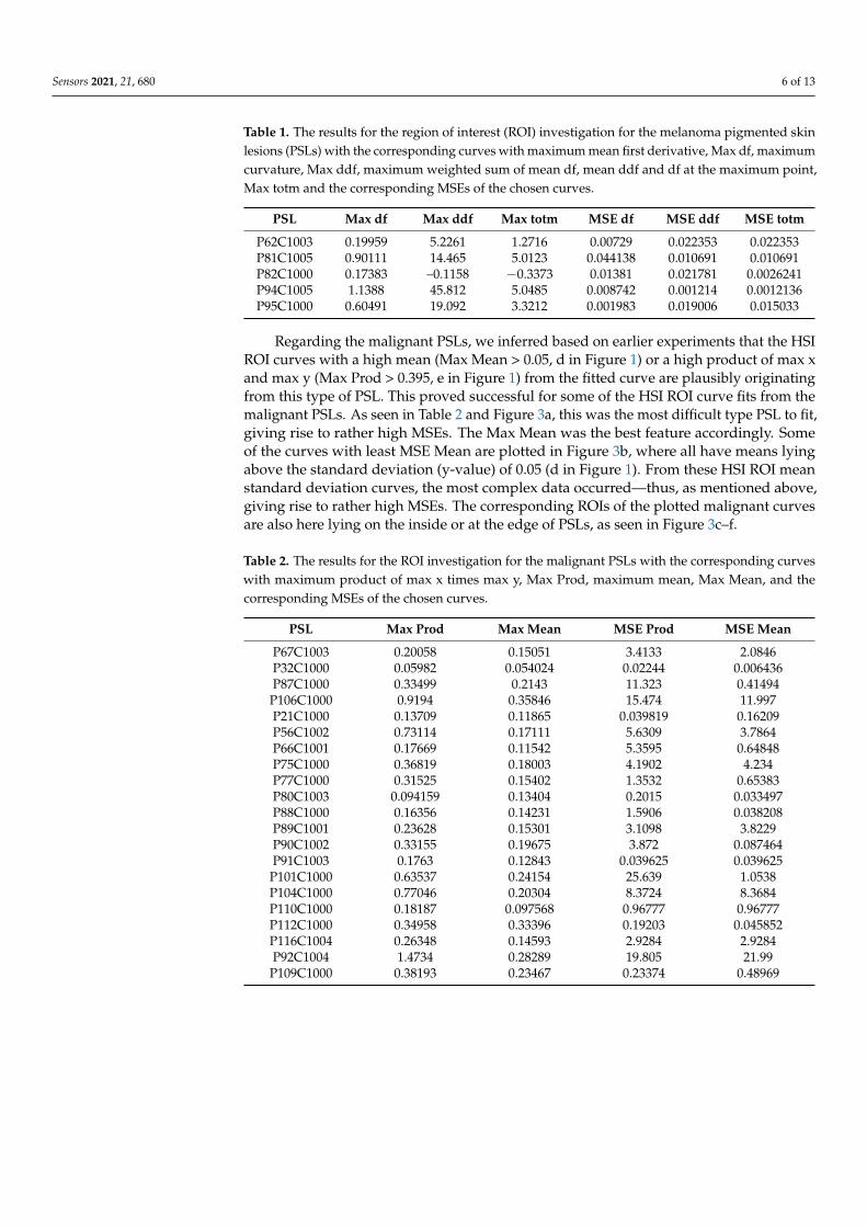
Table 1. The results for the region of interest (ROI) investigation for the melanoma pigmented skinlesions (PSLs) with the corresponding curves with maximum mean first derivative, Max df, maximumcurvature, Max ddf, maximum weighted sum of mean df, mean ddf and df at the maximum point,Max totm and the corresponding MSEs of the chosen curves.

PSL Max df Max ddf Max totm MSE df MSE ddf MSE totm

P62C1003 0.19959 5.2261 1.2716 0.00729 0.022353 0.022353P81C1005 0.90111 14.465 5.0123 0.044138 0.010691 0.010691P82C1000 0.17383 –0.1158 −0.3373 0.01381 0.021781 0.0026241P94C1005 1.1388 45.812 5.0485 0.008742 0.001214 0.0012136P95C1000 0.60491 19.092 3.3212 0.001983 0.019006 0.015033

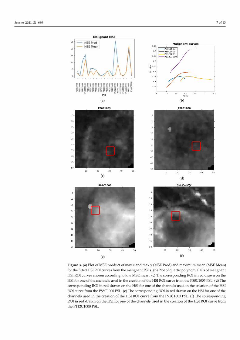
Regarding the malignant PSLs, we inferred based on earlier experiments that the HSIROI curves with a high mean (Max Mean > 0.05, d in Figure 1) or a high product of max xand max y (Max Prod > 0.395, e in Figure 1) from the fitted curve are plausibly originatingfrom this type of PSL. This proved successful for some of the HSI ROI curve fits from themalignant PSLs. As seen in Table 2 and Figure 3a, this was the most difficult type PSL to fit,giving rise to rather high MSEs. The Max Mean was the best feature accordingly. Someof the curves with least MSE Mean are plotted in Figure 3b, where all have means lyingabove the standard deviation (y-value) of 0.05 (d in Figure 1). From these HSI ROI meanstandard deviation curves, the most complex data occurred—thus, as mentioned above,giving rise to rather high MSEs. The corresponding ROIs of the plotted malignant curvesare also here lying on the inside or at the edge of PSLs, as seen in Figure 3c–f.

Table 2. The results for the ROI investigation for the malignant PSLs with the corresponding curveswith maximum product of max x times max y, Max Prod, maximum mean, Max Mean, and thecorresponding MSEs of the chosen curves.

PSL Max Prod Max Mean MSE Prod MSE Mean

P67C1003 0.20058 0.15051 3.4133 2.0846P32C1000 0.05982 0.054024 0.02244 0.006436P87C1000 0.33499 0.2143 11.323 0.41494

P106C1000 0.9194 0.35846 15.474 11.997P21C1000 0.13709 0.11865 0.039819 0.16209P56C1002 0.73114 0.17111 5.6309 3.7864P66C1001 0.17669 0.11542 5.3595 0.64848P75C1000 0.36819 0.18003 4.1902 4.234P77C1000 0.31525 0.15402 1.3532 0.65383P80C1003 0.094159 0.13404 0.2015 0.033497P88C1000 0.16356 0.14231 1.5906 0.038208P89C1001 0.23628 0.15301 3.1098 3.8229P90C1002 0.33155 0.19675 3.872 0.087464P91C1003 0.1763 0.12843 0.039625 0.039625

P101C1000 0.63537 0.24154 25.639 1.0538P104C1000 0.77046 0.20304 8.3724 8.3684P110C1000 0.18187 0.097568 0.96777 0.96777P112C1000 0.34958 0.33396 0.19203 0.045852P116C1004 0.26348 0.14593 2.9284 2.9284P92C1004 1.4734 0.28289 19.805 21.99

P109C1000 0.38193 0.23467 0.23374 0.48969

Sensors 2021, 21, 680 7 of 13

Sensors 2021, 21, x FOR PEER REVIEW  7 of 13  

 

P91C1003  0.1763  0.12843  0.039625  0.039625 

P101C1000  0.63537  0.24154  25.639  1.0538 

P104C1000  0.77046  0.20304  8.3724  8.3684 

P110C1000  0.18187  0.097568  0.96777  0.96777 

P112C1000  0.34958  0.33396  0.19203  0.045852 

P116C1004  0.26348  0.14593  2.9284  2.9284 

P92C1004  1.4734  0.28289  19.805  21.99 

P109C1000  0.38193  0.23467  0.23374  0.48969 

 

 (a) 

 (b) 

 (c)   

(d) 

 (e) 

 (f) 

Figure 3. (a) Plot of MSE product of max x and max y (MSE Prod) and maximum mean (MSE Mean)for the fitted HSI ROI curves from the malignant PSLs. (b) Plot of quartic polynomial fits of malignantHSI ROI curves chosen according to low MSE mean. (c) The corresponding ROI in red drawn on theHSI for one of the channels used in the creation of the HSI ROI curve from the P80C1003 PSL. (d) Thecorresponding ROI in red drawn on the HSI for one of the channels used in the creation of the HSIROI curve from the P88C1000 PSL. (e) The corresponding ROI in red drawn on the HSI for one of thechannels used in the creation of the HSI ROI curve from the P91C1003 PSL. (f) The correspondingROI in red drawn on the HSI for one of the channels used in the creation of the HSI ROI curve fromthe P112C1000 PSL.

Sensors 2021, 21, 680 8 of 13

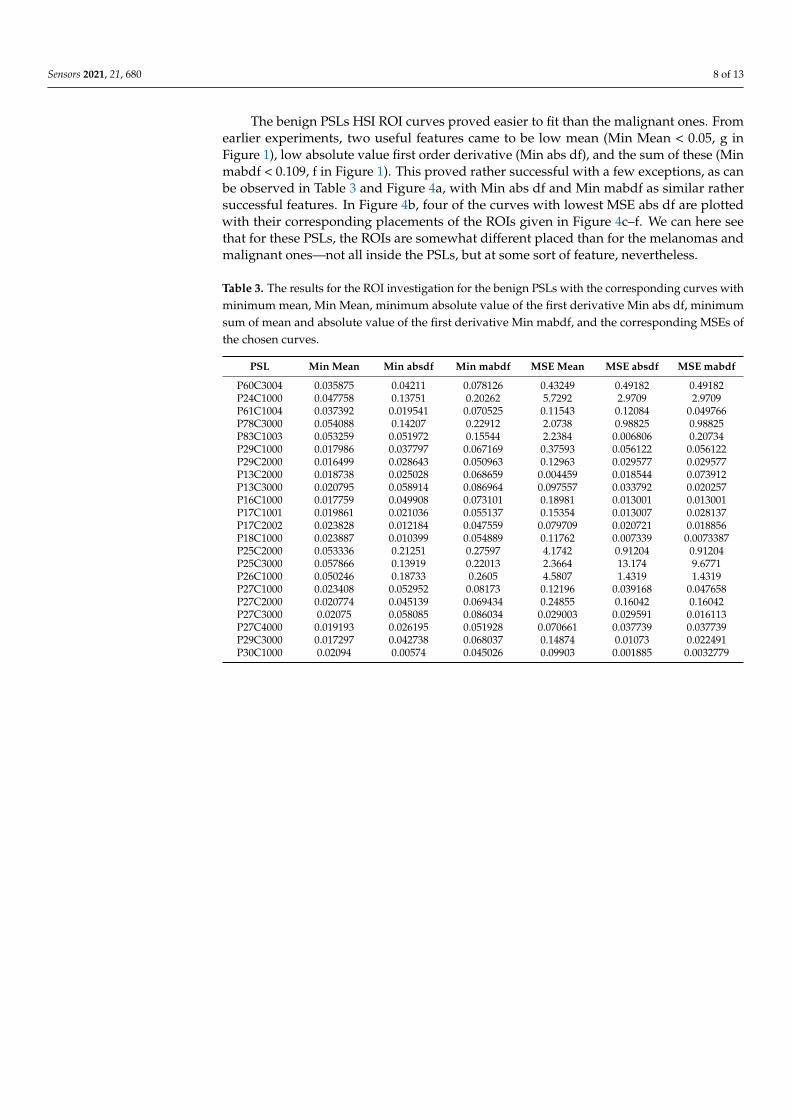
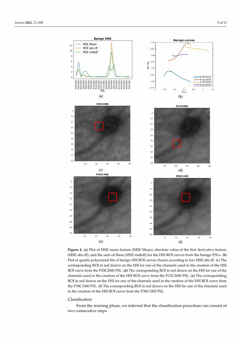
The benign PSLs HSI ROI curves proved easier to fit than the malignant ones. Fromearlier experiments, two useful features came to be low mean (Min Mean < 0.05, g inFigure 1), low absolute value first order derivative (Min abs df), and the sum of these (Minmabdf < 0.109, f in Figure 1). This proved rather successful with a few exceptions, as canbe observed in Table 3 and Figure 4a, with Min abs df and Min mabdf as similar rathersuccessful features. In Figure 4b, four of the curves with lowest MSE abs df are plottedwith their corresponding placements of the ROIs given in Figure 4c–f. We can here seethat for these PSLs, the ROIs are somewhat different placed than for the melanomas andmalignant ones—not all inside the PSLs, but at some sort of feature, nevertheless.

Table 3. The results for the ROI investigation for the benign PSLs with the corresponding curves withminimum mean, Min Mean, minimum absolute value of the first derivative Min abs df, minimumsum of mean and absolute value of the first derivative Min mabdf, and the corresponding MSEs ofthe chosen curves.

PSL Min Mean Min absdf Min mabdf MSE Mean MSE absdf MSE mabdf

P60C3004 0.035875 0.04211 0.078126 0.43249 0.49182 0.49182P24C1000 0.047758 0.13751 0.20262 5.7292 2.9709 2.9709P61C1004 0.037392 0.019541 0.070525 0.11543 0.12084 0.049766P78C3000 0.054088 0.14207 0.22912 2.0738 0.98825 0.98825P83C1003 0.053259 0.051972 0.15544 2.2384 0.006806 0.20734P29C1000 0.017986 0.037797 0.067169 0.37593 0.056122 0.056122P29C2000 0.016499 0.028643 0.050963 0.12963 0.029577 0.029577P13C2000 0.018738 0.025028 0.068659 0.004459 0.018544 0.073912P13C3000 0.020795 0.058914 0.086964 0.097557 0.033792 0.020257P16C1000 0.017759 0.049908 0.073101 0.18981 0.013001 0.013001P17C1001 0.019861 0.021036 0.055137 0.15354 0.013007 0.028137P17C2002 0.023828 0.012184 0.047559 0.079709 0.020721 0.018856P18C1000 0.023887 0.010399 0.054889 0.11762 0.007339 0.0073387P25C2000 0.053336 0.21251 0.27597 4.1742 0.91204 0.91204P25C3000 0.057866 0.13919 0.22013 2.3664 13.174 9.6771P26C1000 0.050246 0.18733 0.2605 4.5807 1.4319 1.4319P27C1000 0.023408 0.052952 0.08173 0.12196 0.039168 0.047658P27C2000 0.020774 0.045139 0.069434 0.24855 0.16042 0.16042P27C3000 0.02075 0.058085 0.086034 0.029003 0.029591 0.016113P27C4000 0.019193 0.026195 0.051928 0.070661 0.037739 0.037739P29C3000 0.017297 0.042738 0.068037 0.14874 0.01073 0.022491P30C1000 0.02094 0.00574 0.045026 0.09903 0.001885 0.0032779

Sensors 2021, 21, 680 9 of 13Sensors 2021, 21, x FOR PEER REVIEW  9 of 13  

 

 (a) 

 (b) 

 (c) 

 (d) 

 (e) 

 (f) 

Figure 4. (a) Plot of MSE mean feature (MSE Mean), absolute value of the first derivative feature 

(MSE abs df), and the sum of these (MSE mabdf) for the HSI ROI curves from the benign PSLs. (b) 

Plot of quartic polynomial fits of benign HSI ROI curves chosen according to low MSE abs df. (c) 

The corresponding ROI in red drawn on the HSI for one of the channels used in the creation of the 

HSI ROI curve from the P29C2000 PSL. (d) The corresponding ROI in red drawn on the HSI for one 

of the channels used  in the creation of the HSI ROI curve from the P13C2000 PSL. (e) The corre‐

sponding ROI in red drawn on the HSI for one of the channels used in the creation of the HSI ROI 

curve from the P18C1000 PSL. (f) The corresponding ROI in red drawn on the HSI for one of the 

channels used in the creation of the HSI ROI curve from the P30C1000 PSL. 

Classification 

From the training phase, we inferred that the classification procedure can consist of 

two consecutive steps. 

Figure 4. (a) Plot of MSE mean feature (MSE Mean), absolute value of the first derivative feature(MSE abs df), and the sum of these (MSE mabdf) for the HSI ROI curves from the benign PSLs. (b)Plot of quartic polynomial fits of benign HSI ROI curves chosen according to low MSE abs df. (c) Thecorresponding ROI in red drawn on the HSI for one of the channels used in the creation of the HSIROI curve from the P29C2000 PSL. (d) The corresponding ROI in red drawn on the HSI for one of thechannels used in the creation of the HSI ROI curve from the P13C2000 PSL. (e) The correspondingROI in red drawn on the HSI for one of the channels used in the creation of the HSI ROI curve fromthe P18C1000 PSL. (f) The corresponding ROI in red drawn on the HSI for one of the channels usedin the creation of the HSI ROI curve from the P30C1000 PSL.

Classification

From the training phase, we inferred that the classification procedure can consist oftwo consecutive steps.

Sensors 2021, 21, 680 10 of 13

First, we identify the curves where the first derivative increases, possibly convergingat maximum value of the HSI ROI curves mean. Additionally, the curves with high meanpositive curvature and less double inflexion points were also identified as melanomas. Inaddition, the sum df + 0.1ddf proved successful (totm).

Then, we find the two clusters of the rest of the curves, such that they can be classifiedas benign or malignant. This is mainly done by choosing what curves have mean abovey = 0.05 (malignant) and below y = 0.05 (benign). For the benign curves, an additionaluseful feature was the sum of the mean of the fitted curve and the mean absolute value ofthe first-order derivative in each point (mabdf).

3.2. Validation and Test Experiment

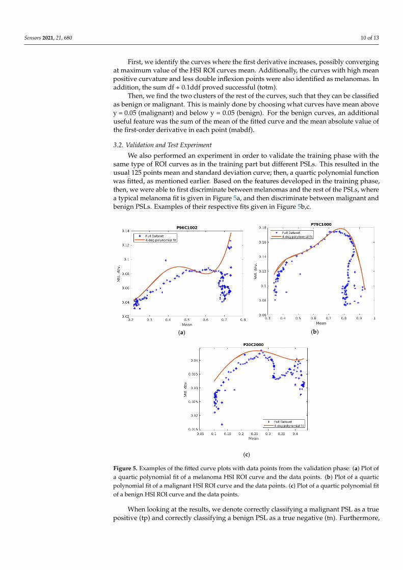
We also performed an experiment in order to validate the training phase with thesame type of ROI curves as in the training part but different PSLs. This resulted in theusual 125 points mean and standard deviation curve; then, a quartic polynomial functionwas fitted, as mentioned earlier. Based on the features developed in the training phase,then, we were able to first discriminate between melanomas and the rest of the PSLs, wherea typical melanoma fit is given in Figure 5a, and then discriminate between malignant andbenign PSLs. Examples of their respective fits given in Figure 5b,c.

Sensors 2021, 21, x FOR PEER REVIEW  10 of 13  

 

First, we identify the curves where the first derivative increases, possibly converging 

at maximum value of the HSI ROI curves mean. Additionally, the curves with high mean 

positive curvature and less double inflexion points were also identified as melanomas. In 

addition, the sum df + 0.1ddf proved successful (totm). 

Then, we find the two clusters of the rest of the curves, such that they can be classified 

as benign or malignant. This is mainly done by choosing what curves have mean above y 

= 0.05 (malignant) and below y = 0.05 (benign). For the benign curves, an additional useful 

feature was the sum of the mean of the fitted curve and the mean absolute value of the 

first‐order derivative in each point (mabdf). 

3.2. Validation and Test Experiment 

We also performed an experiment  in order to validate the training phase with the 

same type of ROI curves as in the training part but different PSLs. This resulted  in the 

usual 125 points mean and standard deviation curve; then, a quartic polynomial function 

was fitted, as mentioned earlier. Based on the features developed in the training phase, 

then, we were able  to  first discriminate between melanomas and  the  rest of  the PSLs, 

where a typical melanoma fit is given in Figure 5a, and then discriminate between malig‐

nant and benign PSLs. Examples of their respective fits given in Figure 5b,c. 

 (a) 

 (b) 

 

(c) 

Figure 5. Examples of the fitted curve plots with data points from the validation phase: (a) Plot of a 

quartic polynomial fit of a melanoma HSI ROI curve and the data points. (b) Plot of a quartic poly‐

nomial fit of a malignant HSI ROI curve and the data points. (c) Plot of a quartic polynomial fit of a 

benign HSI ROI curve and the data points. 

Figure 5. Examples of the fitted curve plots with data points from the validation phase: (a) Plot ofa quartic polynomial fit of a melanoma HSI ROI curve and the data points. (b) Plot of a quarticpolynomial fit of a malignant HSI ROI curve and the data points. (c) Plot of a quartic polynomial fitof a benign HSI ROI curve and the data points.

When looking at the results, we denote correctly classifying a malignant PSL as a truepositive (tp) and correctly classifying a benign PSL as a true negative (tn). Furthermore,

Sensors 2021, 21, 680 11 of 13

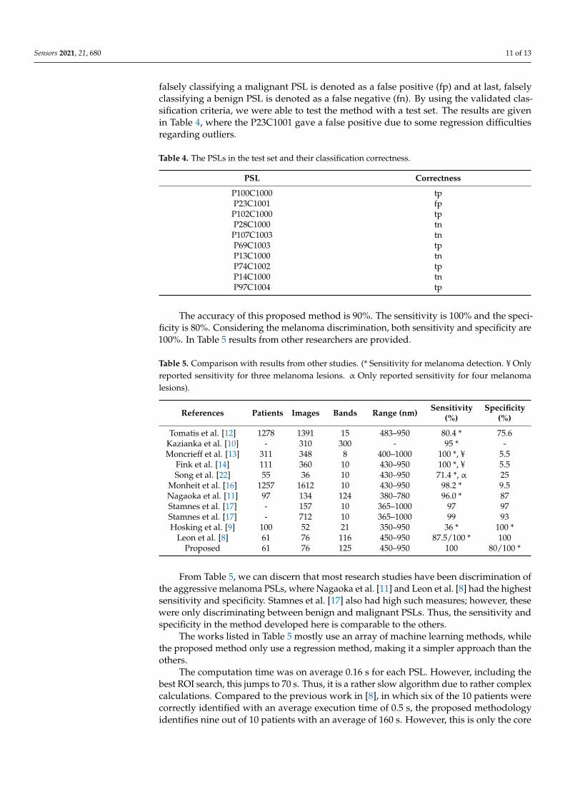
falsely classifying a malignant PSL is denoted as a false positive (fp) and at last, falselyclassifying a benign PSL is denoted as a false negative (fn). By using the validated clas-sification criteria, we were able to test the method with a test set. The results are givenin Table 4, where the P23C1001 gave a false positive due to some regression difficultiesregarding outliers.

Table 4. The PSLs in the test set and their classification correctness.

PSL Correctness

P100C1000 tpP23C1001 fpP102C1000 tpP28C1000 tnP107C1003 tnP69C1003 tpP13C1000 tnP74C1002 tpP14C1000 tnP97C1004 tp

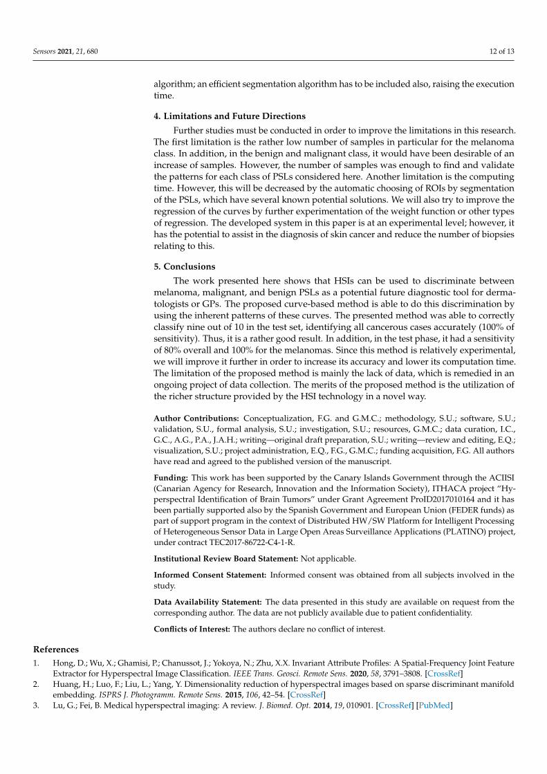
The accuracy of this proposed method is 90%. The sensitivity is 100% and the speci-ficity is 80%. Considering the melanoma discrimination, both sensitivity and specificity are100%. In Table 5 results from other researchers are provided.

Table 5. Comparison with results from other studies. (* Sensitivity for melanoma detection. ¥ Onlyreported sensitivity for three melanoma lesions. α Only reported sensitivity for four melanomalesions).

References Patients Images Bands Range (nm) Sensitivity(%)

Specificity(%)

Tomatis et al. [12] 1278 1391 15 483–950 80.4 * 75.6Kazianka et al. [10] - 310 300 - 95 * -Moncrieff et al. [13] 311 348 8 400–1000 100 *, ¥ 5.5

Fink et al. [14] 111 360 10 430–950 100 *, ¥ 5.5Song et al. [22] 55 36 10 430–950 71.4 *, α 25

Monheit et al. [16] 1257 1612 10 430–950 98.2 * 9.5Nagaoka et al. [11] 97 134 124 380–780 96.0 * 87Stamnes et al. [17] - 157 10 365–1000 97 97Stamnes et al. [17] - 712 10 365–1000 99 93Hosking et al. [9] 100 52 21 350–950 36 * 100 *

Leon et al. [8] 61 76 116 450–950 87.5/100 * 100Proposed 61 76 125 450–950 100 80/100 *

From Table 5, we can discern that most research studies have been discrimination ofthe aggressive melanoma PSLs, where Nagaoka et al. [11] and Leon et al. [8] had the highestsensitivity and specificity. Stamnes et al. [17] also had high such measures; however, thesewere only discriminating between benign and malignant PSLs. Thus, the sensitivity andspecificity in the method developed here is comparable to the others.

The works listed in Table 5 mostly use an array of machine learning methods, whilethe proposed method only use a regression method, making it a simpler approach than theothers.

The computation time was on average 0.16 s for each PSL. However, including thebest ROI search, this jumps to 70 s. Thus, it is a rather slow algorithm due to rather complexcalculations. Compared to the previous work in [8], in which six of the 10 patients werecorrectly identified with an average execution time of 0.5 s, the proposed methodologyidentifies nine out of 10 patients with an average of 160 s. However, this is only the core

Sensors 2021, 21, 680 12 of 13

algorithm; an efficient segmentation algorithm has to be included also, raising the executiontime.

4. Limitations and Future Directions

Further studies must be conducted in order to improve the limitations in this research.The first limitation is the rather low number of samples in particular for the melanomaclass. In addition, in the benign and malignant class, it would have been desirable of anincrease of samples. However, the number of samples was enough to find and validatethe patterns for each class of PSLs considered here. Another limitation is the computingtime. However, this will be decreased by the automatic choosing of ROIs by segmentationof the PSLs, which have several known potential solutions. We will also try to improve theregression of the curves by further experimentation of the weight function or other typesof regression. The developed system in this paper is at an experimental level; however, ithas the potential to assist in the diagnosis of skin cancer and reduce the number of biopsiesrelating to this.

5. Conclusions

The work presented here shows that HSIs can be used to discriminate betweenmelanoma, malignant, and benign PSLs as a potential future diagnostic tool for derma-tologists or GPs. The proposed curve-based method is able to do this discrimination byusing the inherent patterns of these curves. The presented method was able to correctlyclassify nine out of 10 in the test set, identifying all cancerous cases accurately (100% ofsensitivity). Thus, it is a rather good result. In addition, in the test phase, it had a sensitivityof 80% overall and 100% for the melanomas. Since this method is relatively experimental,we will improve it further in order to increase its accuracy and lower its computation time.The limitation of the proposed method is mainly the lack of data, which is remedied in anongoing project of data collection. The merits of the proposed method is the utilization ofthe richer structure provided by the HSI technology in a novel way.

Author Contributions: Conceptualization, F.G. and G.M.C.; methodology, S.U.; software, S.U.;validation, S.U., formal analysis, S.U.; investigation, S.U.; resources, G.M.C.; data curation, I.C.,G.C., A.G., P.A., J.A.H.; writing—original draft preparation, S.U.; writing—review and editing, E.Q.;visualization, S.U.; project administration, E.Q., F.G., G.M.C.; funding acquisition, F.G. All authorshave read and agreed to the published version of the manuscript.

Funding: This work has been supported by the Canary Islands Government through the ACIISI(Canarian Agency for Research, Innovation and the Information Society), ITHACA project “Hy-perspectral Identification of Brain Tumors” under Grant Agreement ProID2017010164 and it hasbeen partially supported also by the Spanish Government and European Union (FEDER funds) aspart of support program in the context of Distributed HW/SW Platform for Intelligent Processingof Heterogeneous Sensor Data in Large Open Areas Surveillance Applications (PLATINO) project,under contract TEC2017-86722-C4-1-R.

Institutional Review Board Statement: Not applicable.

Informed Consent Statement: Informed consent was obtained from all subjects involved in thestudy.

Data Availability Statement: The data presented in this study are available on request from thecorresponding author. The data are not publicly available due to patient confidentiality.

Conflicts of Interest: The authors declare no conflict of interest.

References1. Hong, D.; Wu, X.; Ghamisi, P.; Chanussot, J.; Yokoya, N.; Zhu, X.X. Invariant Attribute Profiles: A Spatial-Frequency Joint Feature

Extractor for Hyperspectral Image Classification. IEEE Trans. Geosci. Remote Sens. 2020, 58, 3791–3808. [CrossRef]2. Huang, H.; Luo, F.; Liu, L.; Yang, Y. Dimensionality reduction of hyperspectral images based on sparse discriminant manifold

embedding. ISPRS J. Photogramm. Remote Sens. 2015, 106, 42–54. [CrossRef]3. Lu, G.; Fei, B. Medical hyperspectral imaging: A review. J. Biomed. Opt. 2014, 19, 010901. [CrossRef] [PubMed]

Sensors 2021, 21, 680 13 of 13

4. Johansen, T.H.; Møllersen, K.; Ortega, S.; Fabelo, H.; Garcia, A.; Callico, G.M.; Godtliebsen, F. Recent advances in hyperspectralimaging for melanoma detection. Wiley Interdiscip. Rev. Comput. Stat. 2019, 12, e1465. [CrossRef]

5. Bray, F.; Ferlay, J.; Soerjomataram, I.; Siegel, R.L.; Torre, L.A.; Jemal, A. Global cancer statistics 2018: GLOBOCAN estimates ofincidence and mortality worldwide for 36 cancers in 185 countries. CA Cancer J. Clin. 2018, 68, 394–424. [CrossRef]

6. LeBoit, P.E.; Burg, G.; Weedon, D.; Sarasin, A. Pathology & Genetics Skin Tumors; World Health Organization: Geneve, Switzerland,2006.

7. Tsao, H.; Olazagasti, J.M.; Cordoro, K.M.; Brewer, J.D.; Taylor, S.C.; Bordeaux, J.S.; Chren, M.-M.; Sober, A.J.; Tegeler, C.; Bhushan,R.; et al. Early detection of melanoma: Reviewing the ABCDEs American Academy of Dermatology Ad Hoc Task Force for theABCDEs of Melanoma. J. Am. Acad. Dermatol. 2015, 72, 717–723. [CrossRef]

8. Leon, R.; Martinez, B.; Fabelo, H.; Ortega, S.; Melian, V.; Castaño, I.; Carretero, G.; Almeida, P.; Garcia, A.; Quevedo, E.; et al.Non-Invasive Skin Cancer Diagnosis Using Hyperspectral Imaging for In-Situ Clinical Support. J. Clin. Med. 2020, 9, 1662.[CrossRef] [PubMed]

9. Hosking, A.-M.; Coakley, B.J.; Chang, D.; Talebi-Liasi, F.; Lish, S.; Lee, S.W.; Zong, A.M.; Moore, I.; Browning, J.; Jacques, S.L.;et al. Hyperspectral imaging in automated digital dermoscopy screening for melanoma. Lasers Surg. Med. 2019, 51, 214–222.[CrossRef] [PubMed]

10. Kazianka, H.; Leitner, R.; Pilz, J. Segmentation and classification of hyper-spectral skin data. In Studies in Classification, DataAnalysis, and Knowledge Organization; Springer: Berlin/Heidelberg, Germany, 2008.

11. Nagaoka, T.; Nakamura, A.; Kiyohara, Y.; Sota, T. Melanoma Screening System Using Hyperspectral Imager Attached to ImagingFiberscope. In Proceedings of the Annual International Conference of the IEEE Engineering in Medicine and Biology Society, SanDiego, CA, USA, 28 August–1 September 2012.

12. Tomatis, S.; Carrara, M.; Bono, A.; Bartoli, C.; Lualdi, M.; Tragni, G.; Colombo, A.; Marchesini, R. Automated melanoma detectionwith a novel multispectral imaging system: Results of a prospective study. Phys. Med. Biol. 2005, 50, 1675–1687. [CrossRef][PubMed]

13. Moncrieff, M.D.; Cotton, S.; Claridge, E.; Hall, P. Spectrophotometric intracutaneous analysis: A new technique for imagingpigmented skin lesions. Br. J. Dermatol. 2002, 146, 448–457. [CrossRef] [PubMed]

14. Fink, C.; Jaeger, C.; Jaeger, K.; Haenssle, H.A. Diagnostic performance of the MelaFind device in a real-life clinical setting. J. Dtsch.Dermatol. Ges. 2017, 15, 414–419. [CrossRef] [PubMed]

15. Elbaum, M.; Kopf, A.W.; Rabinovitz, H.S.; Langley, R.G.B.; Kamino, H.; Mihm, M.C.; Sober, A.J.; Peck, G.L.; Bogdan, A.;Gutkowicz-Krusin, D.; et al. Automatic differentiation of melanoma from melanocytic nevi with multispectral digital dermoscopy:A feasibility study. J. Am. Acad. Dermatol. 2001, 44, 207–218. [CrossRef] [PubMed]

16. Monheit, G.; Cognetta, A.B.; Ferris, L.; Rabinovitz, H.; Gross, K.; Martini, M.; Grichnik, J.M.; Mihm, M.; Prieto, V.G.; Googe, P.;et al. The performance of MelaFind: A prospective multicenter study. Arch. Dermatol. 2011, 147, 188–194. [CrossRef] [PubMed]

17. Stamnes, J.J.; Ryzhikov, G.; Biryulina, M.; Hamre, B.; Zhao, L.; Stamnes, K. Optical detection and monitoring of pigmented skinlesions. Biomed. Opt. Express 2017, 8, 2946–2964. [CrossRef] [PubMed]

18. Abadi, M.; Barham, P.; Chen, J.; Chen, Z.; Davis, A.; Dean, J.; Devin, M.; Ghemawat, S.; Irving, G.; Isard, M.; et al. TensorFlow: ASystem for Large-Scale Machine Learning. In Proceedings of the 12th USENIX Symposium on Operating Systems Design andImplementation, Savannah, GA, USA, 2–4 November 2016; pp. 265–283.

19. Li, S.; Song, W.; Fang, L.; Chen, Y.; Ghamisi, P.; Benediktsson, J.A. Deep learning for hyperspectral image classification: Anoverview. IEEE Trans. Geosci. Remote Sens. 2019, 57, 6690–6709. [CrossRef]

20. Fabelo, H.; Carretero, G.; Almeida, P.; Garcia, A.; Hernandez, J.A.; Godtliebsen, F.; Melian, V.; Martinez, B.; Beltran, P.; Ortega,S.; et al. Dermatologic Hyperspectral Imaging System for Skin Cancer Diagnosis Assistance. In Proceedings of the 2019 34thConference on Design of Circuits and Integrated Systems, Bilbao, Spain, 20–22 November 2019.

21. Holland, P.W.; Welsch, R.E. Robust regression using iteratively reweighted least-squares. Commun. Stat. Theory Methods 1977, 6,813–827. [CrossRef]

22. Song, E.; Grant-Kels, J.M.; Swede, H.; D’Antonio, J.L.; Lachance, A.; Dadras, S.S.; Kristjansson, A.K.; Ferenczi, K.; Makkar,H.S.; Rothe, M.J. Paired comparison of the sensitivity and specificity of multispectral digital skin lesion analysis and reflectanceconfocal microscopy in the detection of melanoma in vivo: A cross-sectional study. J. Am. Acad. Dermatol. 2016, 75, 1187–1192.[CrossRef] [PubMed]