Embed Size (px)
Citation preview

Nick Borer MATH 6514 Final Presentation
Design and Analysis of a Low Reynolds Number Airfoil
Prepared for Dr. J. McCuanMATH 6514: Industrial Math
Presented by Nick Borer

Nick Borer MATH 6514 Final Presentation
Airfoil Design
• In the past, airfoils were designed experimentally and catalogued for future use
• The advent of the digital computer has facilitated custom airfoil design for a given wing planform
• There are several approaches to custom airfoil design– Trial and error– Optimization methods (automated trial and error)– Inverse methods
• My work focuses on the optimization method because I am very familiar with optimization techniques

Nick Borer MATH 6514 Final Presentation
Design Criteria
• The application in mind is for a low-Reynolds number airfoil that will operate on a flying wing UAV
• Reynolds numbers will range between 200,000 and 700,000 for level flight– Airfoil should be designed to operate well between
100,000 and 1,000,000
• This said, the actual viscous calculations do not appear in the design process!– Viscous effects calculated after the design process– Pressure distributions chosen via heuristics for “good”
low-Reynolds number design

Nick Borer MATH 6514 Final Presentation
Design Plot for UAV
0 0.5 1 1.5 2 2.5 3 3.5 4 4.5 50
0.2
0.4
0.6
0.8
1
1.2
WTO/S
T SL/W
TO 80
70
60
50
40
cruise speed contours (MPH)
120 ft. ground roll
T SL
/ WTO
WTO / S

Nick Borer MATH 6514 Final Presentation
Approach• Determine airfoil geometry from input pressure
distribution via incompressible, inviscid analyses– Ideal application for the vortex panel method– Although assumed incompressible, moderate amounts of
compressibility can be predicted via Prandtl-Glauert or Karmen-Tsien compressibility corrections (stretch of geometry in x-direction)
• Compare inviscid results to viscous results post-design
• Three analysis routines tested– Custom vortex-panel code written in Matlab– XFOIL (inviscid only; used as benchmark)– XFOIL (viscous; vortex-panel method with boundary
layer analysis)

Nick Borer MATH 6514 Final Presentation
Vortex Panel Method: Theory
• The vortex panel method belongs to a more general class of analyses known as panel methods– All panel methods rely on a superposition of elementary
flows in potential (incompressible, inviscid) flow to solve a given problem
– “Vortex” panel method implies the use of vortex and uniform flows to solve the problem
• It all starts with the 2D incompressible continuity equation
0=∂∂
+∂∂
yv
xu

Nick Borer MATH 6514 Final Presentation
Vortex Panel Method: Theory
• Stream function (flow abstraction)
• Into continuity, get Laplace’s Equation
• Elemenary solution to vortex and uniform flow
vx
uy
=∂Ψ∂
−=∂Ψ∂ ;
02
2
2
2
=∂Ψ∂
+∂Ψ∂
yx
( )rvortex ln2πΓ
=Ψ
yVuniform ∞=Ψ

Nick Borer MATH 6514 Final Presentation
Vortex Panel Method: Theory
• Break into components along a streamline to get
• Evaluated over n segments (panels), this becomes
• The integral in the middle can be evaluated analytically, and together are known as the aerodynamic influence coefficients
( ) 0ln21
000 =−−−−=Ψ ∫∞∞ Cdsrrxvyu γπ
( ) 0ln21
00,0 =−−−− ∑ ∫
=∞∞ Cdsrrxvyu
n
j j
jii π
γ
( )∫ −= 00, ln21 dsrrA ji π

Nick Borer MATH 6514 Final Presentation
Vortex Panel Method: Theory
• Now we have n equations and n+1 unknowns, so we add in the Kutta condition
• Finally, we have a system of n+1 equations and n+1 unknowns that can be easily inverted and solved
0,01,0 =+ nγγ
01
,0, =−−− ∑=
∞∞ CAxvyun
jjjiii γ
lowerTEupperTE −−−= 00 γγ

Nick Borer MATH 6514 Final Presentation
Validation of Panel Code
• All three panel codes (Matlab, XFOIL-inviscid, and XFOIL-viscous) were compared against trusted experimental data for a NACA 0015 airfoil
• Conditions (when applicable):– α = 5°– Re = 1,950,000– M = 0.29
0
0.2
0.4
0.6
0.8
1
1.2
1.4
1.6
0 2 4 6 8 10 12
alpha (deg)
Cl
experiment
Matlab, inviscid
XFOIL, inviscid
XFOIL, viscous

Nick Borer MATH 6514 Final Presentation
Pressure Distribution Comparison
• All three methods yielded similar results for output pressure distribution
-2.5
-2
-1.5
-1
-0.5
0
0.5
10 0.1 0.2 0.3 0.4 0.5 0.6 0.7 0.8 0.9 1
x/c
Cp
Matlab, inviscid
XFOIL, inviscid
XFOIL, viscous

Nick Borer MATH 6514 Final Presentation
Optimization Setup• Design method
• Optimizer used: fmincon– Sequential Quadratic Programming (SQP) optimizer– capable of handling nonlinear constraints
• Design variables consist of:– multipliers to bump functions (coefficients)– upper and lower airfoil scaling factors– design angle of attack (incidence)
Target PressureDistribution
Seed Airfoil
Main ProgramPre/Post Processor
Optimizer
Analysis
Criteria Met?
No
Yes Exit
current pressure distribution
current design variables
new pressure distribution
new design variables
Nick Borer MATH 6514 Final Presentation
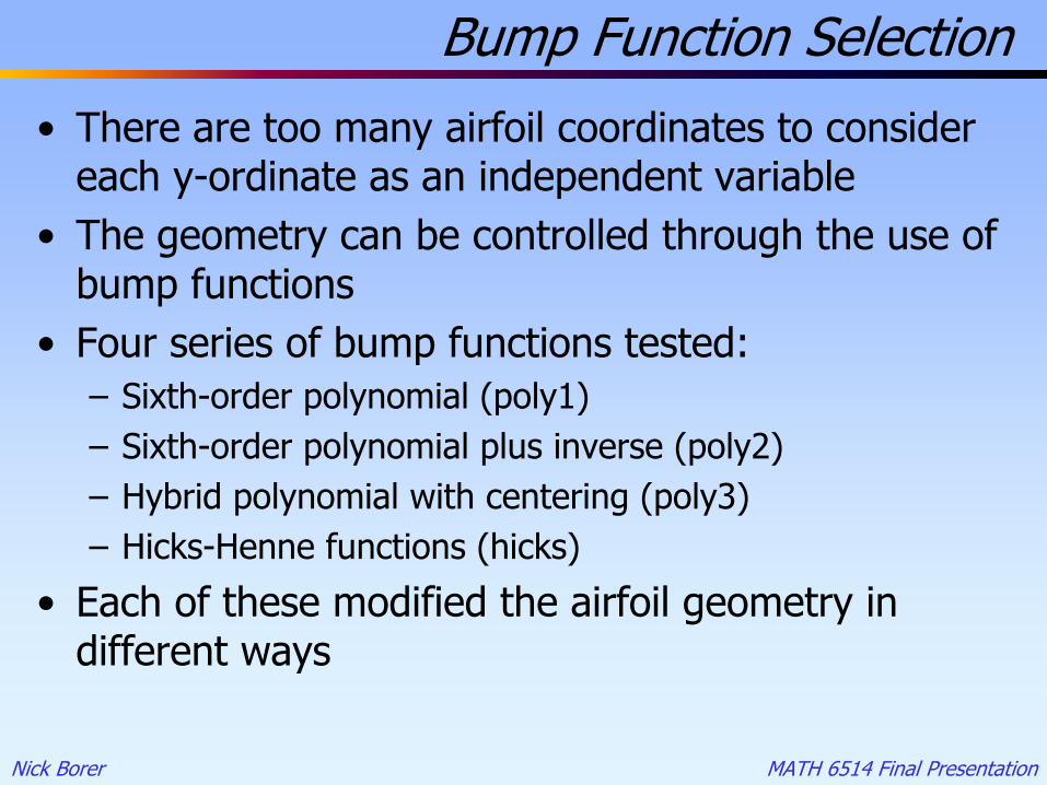
Bump Function Selection
• There are too many airfoil coordinates to consider each y-ordinate as an independent variable
• The geometry can be controlled through the use of bump functions
• Four series of bump functions tested:– Sixth-order polynomial (poly1)– Sixth-order polynomial plus inverse (poly2)– Hybrid polynomial with centering (poly3)– Hicks-Henne functions (hicks)
• Each of these modified the airfoil geometry in different ways

Nick Borer MATH 6514 Final Presentation
P(x) = poly1
0
0.1
0.2
0.3
0.4
0.5
0.6
0.7
0.8
0.9
1
0 0.1 0.2 0.3 0.4 0.5 0.6 0.7 0.8 0.9 1
x
P(x)

Nick Borer MATH 6514 Final Presentation
P(x) = poly2
0
0.1
0.2
0.3
0.4
0.5
0.6
0.7
0.8
0.9
1
0 0.1 0.2 0.3 0.4 0.5 0.6 0.7 0.8 0.9 1
x
P(x)

Nick Borer MATH 6514 Final Presentation
P(x) = poly3
0
0.1
0.2
0.3
0.4
0.5
0.6
0.7
0.8
0.9
1
0 0.1 0.2 0.3 0.4 0.5 0.6 0.7 0.8 0.9 1
x
P(x)

Nick Borer MATH 6514 Final Presentation
P(x) = hicks
0
0.1
0.2
0.3
0.4
0.5
0.6
0.7
0.8
0.9
1
0 0.1 0.2 0.3 0.4 0.5 0.6 0.7 0.8 0.9 1
x
P(x)

Nick Borer MATH 6514 Final Presentation
Design Method Validation
• Wanted to check if the design algorithm would converge to a known airfoil given the appropriate pressure distribution– NACA 4412 airfoil at α = 0°, M = 0.5– Pressure distribution generated from Matlab panel code
to eliminate experimental noise
• Started with two seed airfoils of different families– NACA 0012 (symmetric, same thickness form as 4412)– NACA 23015 (cambered, different thickness form)
• This also provided a way to see which bump function was the most efficient and which was the most robust

Nick Borer MATH 6514 Final Presentation
Design Validation: Results
• Validation found some bugs in the code• All three polynomial bump functions converged to
the correct geometry• The Hicks-Henne functions did not converge
properly• Efficiency: number
of function callsfor 0012 airfoil
0.1
1
10
10 100 1000 10000
function calls
obje
ctiv
e fu
nctio
n
poly1poly2poly3hicks

Nick Borer MATH 6514 Final Presentation
Design Validation: Results
• Efficiency for 23015 seed airfoil
• These results point to poly3 as the most robust set of bump functions
0.1
1
10
10 100 1000 10000
function calls
obje
ctiv
e fu
nctio
n
poly1poly2poly3hicks

Nick Borer MATH 6514 Final Presentation
Design Studies
• Created two input pressure distributions for this speed regime
• Laminar flow: “rooftop” pressure distribution delays adverse pressure gradient, thus delaying pressure-induced transition– Unfortunately, this typically results in a highly rear-
loaded airfoil, which can increase trim drag
• Flying wing: “reflex” pressure distribution used to trim out nose-down pitching moment at design conditions– This necessitates large changes in pressure on both
surfaces of the airfoil, thus making laminar flow difficult to achieve

Nick Borer MATH 6514 Final Presentation
Input Pressure Distributions
• Defined via heuristics and a generic polynomial to ensure that the distributions were smooth
• Later studies will define these from desired wing lift distributions: elliptic spanwise, reflex chordwise, etc.
-1.5
-1
-0.5
0
0.5
10 0.1 0.2 0.3 0.4 0.5 0.6 0.7 0.8 0.9 1
x/c
cp(x
/c)
reflex
rooftop

Nick Borer MATH 6514 Final Presentation
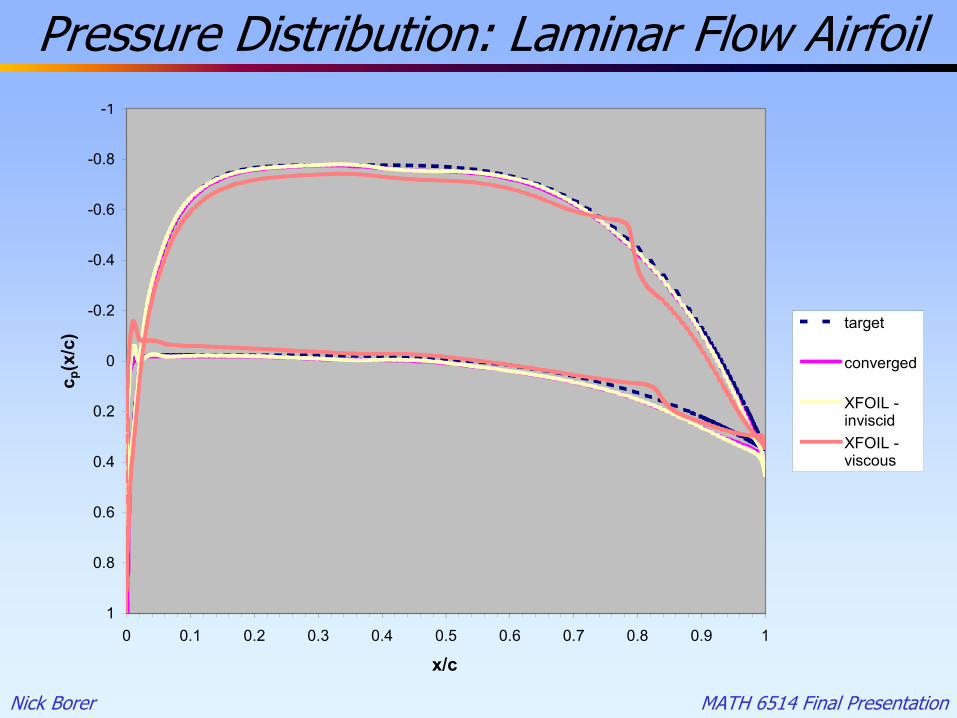
Results
• Both cases converged, and the results were compared against the XFOIL solutions
parameter target converged inviscid viscousCl 0.6000 0.6066 0.6093 0.5322Cm * -0.1387 -0.1394 -0.1225Cd 0.0000 0.0008 -0.0003 0.0055Cl 0.6000 0.6169 0.6153 0.5637Cm 0.0000 -0.0043 -0.0078 0.0027Cd 0.0000 0.0008 -0.0002 0.0081re
flex
roof
top
XFOILMatlab
Nick Borer MATH 6514 Final Presentation
Pressure Distribution: Laminar Flow Airfoil-1
-0.8
-0.6
-0.4
-0.2
0
0.2
0.4
0.6
0.8
10 0.1 0.2 0.3 0.4 0.5 0.6 0.7 0.8 0.9 1
x/c
c p(x
/c) target
converged
XFOIL -inviscidXFOIL -viscous

Nick Borer MATH 6514 Final Presentation
Pressure Distribution: Reflex Airfoil-1.5
-1
-0.5
0
0.5
10 0.1 0.2 0.3 0.4 0.5 0.6 0.7 0.8 0.9 1
x/c
c p(x
/c)
target
converged
XFOIL -inviscidXFOIL -viscous

Nick Borer MATH 6514 Final Presentation
Converged Airfoil Shapes
-0.3
-0.2
-0.1
0
0.1
0.2
0.3
0 0.1 0.2 0.3 0.4 0.5 0.6 0.7 0.8 0.9 1
x/c
y/c
reflex
rooftop

Nick Borer MATH 6514 Final Presentation
Comments and Future Work
• The airfoils that resulted from this design code reflected the physics of the design problem– The laminar airfoil has a relatively small leading edge
radius and even thickness form– The reflex airfoil has noticeable positive camber near the
leading edge and reflex camper near the trailing edge
• Design method would be better if it could be coupled with a boundary layer analysis– Panel code geometry could update with boundary layer
displacement thickness
• This 2D design tool can be coupled with a 3D analysis for efficient wing design
Nick Borer MATH 6514 Final Presentation
Backups

Nick Borer MATH 6514 Final Presentation
Drag Polars
0
0.002
0.004
0.006
0.008
0.01
0.012
0.014
0.016
0.018
0.02
0 0.2 0.4 0.6 0.8 1 1.2 1.4
Cl
Cd rooftop
reflex

Nick Borer MATH 6514 Final Presentation
Lift Curves
-0.2
0
0.2
0.4
0.6
0.8
1
1.2
1.4
-6 -4 -2 0 2 4 6 8 10
alpha (deg)
Cl rooftop
reflex

Nick Borer MATH 6514 Final Presentation
Moment Curves
-0.16
-0.14
-0.12
-0.1
-0.08
-0.06
-0.04
-0.02
0
0.02
-6 -4 -2 0 2 4 6 8 10
alpha (deg)
Cm rooftop
reflex