Design and Analysis of DNA Microarray Investigations - Biometric

r-

Richard M. SimonLisa M. McShaneGeorge W. Wright

--

Edward L. KornMichael D. RadmacherYingdong Zhao

Design and Analysis ofDNA MicroatrayInvestigations

With 58 Figures, 15 in Full color

Springer

t,

r- --

Richard M. SimonEdward L. KomLisa M. McShaneGeorge W. WrightYingdong ZhaoBiometrc Research Branch

National Cancer Institute9000 Rockvile Pike

MSC 7434Bethesda, MD 20892-7434

Michael D. RadmacherDeparments of Mathematics

& BiologyKenyon CollegeGambier, OR 43022

Series Editors

K. Dietz

Institut fUr Medizinische BiometreUniversitat TUbingenWestbahnhofstrasse 55D-72070 TUbingen

Germany

J. SametDepartent of Epidemiology

School of Public HealthJohns Hopkins University615 Wolfe StreetBaltimore, MD 21205-2103USA

M.GailNational Cancer InstituteRockvile, MD 20892USA

K. KrckebergLe ChateletF-63270 ManglieuFrance

A. TsiatisDeparment of StatisticsNort Carolina State UniversityRaleigh, NC 27695USA

Library of Congress Cataloging-in-Publication DataDesign and analysis of DNA microaray investigations / Richard M. Simon. . . (et al.).

p. em. - (Statistics for biology and health)

ISBN 0-387-00135-2 (hbk. ; alk. paper)i. DNA microarrays-Statistical methods. i. Simon, Richard M., 1943- II. Senes.

QP624.5.D726D475 20035728'65--c21 2003054790ISBN 0-387-00135-2 Printed on acid-free paper.

This work was created by U.S. government employees as part of their offcial duties and is a U.S.government work as that term is defined by U.S. Copyright Law.

Printed in the United States of America.

987654321 SPIN 10898178

www.springer-ny.com

Springer-Verlag New York Berlin HeidelbergA member of BertelsmannSpringer Science+Business Media GmbH

-ir-

Statistics for Biölogy and HealthSeries EditorsK. Dietz, M. Gail, K. Knckeberg, J. Samet, A. Tsiatis

SpringerNew YorkBerlin

. Heidelberg

Hong KongLondonMilanParisTokyo

Acknowledgments

We thank our colleagues at the National Cancer Institute who have given usthe opportunity to become involved in cancer genomics, and to contribute todiscovery of a new generation of therapeutics based on improved knowledgeof tumor biology. We particularly thank Dr. Robert Wittes for supportingthe establishment of the Molecular Statistics and Bioinformatics Section ofthe Biometric Research Branch and providing it with the independence todevelop expertise, conduct independent research, and establish a unique mul-tidisciplinary environment in which methodologists and experimentalists caninteract.

We thank Amy Peng Lam for her development of BRB-ArrayTools incollaboration with Richard Simon, and for her many contributions to ourmicroarray analyses. Thanks to Dr. Ming-Chung Li for excellent statisticalcomputing support, to Dr. James P. Brody for permission to use Figure 3.1,to the National Human Genome Research Institute for ilustrations from theirTalking Glossary website, to Drs. Tatiana Dracheva, Jin Jen, and Joanna'Shih for providing Affmetrix GeneChipTM images, to Mr. Erik Marchese atAffymetrix for technical consultation, and to Dr. Laura Lee Johnson for acareful reading of an earlier draft.

, '(\I ~..

/ÓC

Contents

Acknowledgments ............................................. v

1 Introduction. . . . . . . . . . . . . . . . . . . . . . . . . . . . . . . . . . . . . . . . . . . . . . . 1

2 DNA Microarray Technology.............................. 52.1 Overview............................................... 5

2.2 Measuring Label Intensity . . . . . . . . . . . . . . . . . . . . . . . . . . . . . . . . 52.3 Labeling Methods ... . . . . . . . . . . . . . . . . . . . . . . . . . . . . . . . . . . . . 62.4 Printed Microarrays ..................................... 7

2.5 Affymetrix GeneChip ™ Arrays . . . . . . . . . . . . . . . . . . . . . . . . . .. 92.6 Other Microarray Platforms. . . . .. . . . . .. . . . . . . . . . .. . . . . . .. 10

3 Design of DNA Microarray Experiments. . . . . . . . . . . . . . . . . .. 113.1 Introduction............................................ 11

3.2 Study Objectives. . . . . . . . . . . . . . . . . . . . . . . . . . . . . . . . . . . . . . .. 123.2.1 Class Comparison . . . . . . . . . . . . . . . . . . . . . . . . . . . . . . . .. 123.2.2 Class Prediction. . . . . . . . . . . . . . . . . . . . . . . . . . . . . . . . . .. 133.2.3 Class Discovery. . . . . . . . . . . . . . . . . . . . . . . . . . . . . . . . . .. 133.2.4 Pathway Analysis ................................. 13

3.3 Comparing Two RNA Samples. .. . . . . . . . . . . . . . . . . . . . . . . . .. 133.4 Sources of Variation and Levels of ~plication. . . . . . . . . . . . . .. 143.5 Pooling of Samples ...................................... 16

3.6 Pairing Samples on Dual-Label Microarrays. . . . . . . . . . . . . . . .. 173.6.1 The Reference Design. . . . . . . . . . . . . . . . . . . . . . . . . . . . .. 173.6.2 The Balanced Block Design. . . . . . . . . . . . . . . . . . . . . . . .. 193.6.3 The Loop Design. . . . . . . . . . . . . . . . . . . . . . . . . . . . . . . . .. 20

3.7 Reverse Labeling (Dye Swap) ............................. 21

3.8 Number of Biological Replicates Needed. . . . .. . . . . . . . . . . . . .. 23

vii Contents

4 Image Analysis . . . . . . . . . . . . . . . . . . . . . . . . . . . . . . . . . . . . . . . . . . .. 294.1 Image Generation. . . . . . . .. . . . . . . . . . .. . . . . .. . . . . . . .. . . . .. 294.2 Image Analysis for cDNA Microarrays ..................... 30

4.2.1 Image Display. . .. . . .. . . . . . . . . . . . . . . . . . . . . . . . . . . .. 304.2.2 Gridding......................................... 30

4.2.3 Segmentation..................................... 31

4.2.4 Foreground Intensity Extraction. . . . . . . . . . . . . . . . . . . .. 324.2.5 Background Correction. . . . . . . . . . . . . . . . . . . . . . . . . . . .. 334.2.6 Image Output File. . . . . . . . . . . . . . . . . . . . . . . . . . . . . . . .. 34

4.3 Image Analysis for Affmetrix GeneChip ™ ................ 35

5 Quality Control. . . . . . . . . . . . . . . . . . . . . . . . . . . . . . . . . . . . . . . . . . .. 395.1 Introduction............................................ 39

5.2 Probe-Level Quality Control for Two-Color Arrays. . . . . . . . . .. 405.2.1 Visual Inspection of the Image File. . . . .. . . . .. . . . . ... 405.2.2 Spots Flagged at Image Analysis ,. . . . . . . . . . . . . . . . . .. 405.2.3 Spot Size. . . . . . . . . . . . . . . . . . . . . . . . . . . . . . . . . . . . . . . .. 415.2.4 Weak Signal . . . . . . . . . . . . . . . . . . . . . . . . . . . . . . . . . . . . .. 425.2.5 Large Relative Background Intensity. . . . . . . . . . . . . . . .. 43

5.3 Gene Level Quality Control for Two-Color Arrays ........... 44

5.3.1 Poor Hybridization and Printing.. . . . . . . . . . . . . . . . . .. 455.3.2 Probe Quality Control Based on Duplicate Spots. . . . .. 455.3.3 Low Variance Genes . . . . . . . . . . . . . . . . . . . . . . . . . . . . . .. 46

5.4 Array-Level Quality Control for Two-Color Arrays. .. . . . . . ... 475.5 Quality Control for GeneChipTM Arrays. . . . . . . . . . . . . . . . . . .. 485.6 Data Imputation ... . . . . . . . . . . . . . . . . . . .. . . . . . . . . . . . . . . . .. 50

6 Array Normalization..... .. .... .... . ............ .. .. ... .... 536.1 Introduction............................................ 53

6.2 Choice of Genes for Normalization. . . . . .. ... . . . . . . . . . . . . .,. 536.2.1 Biologically Defined Housekeeping Genes. . . . . .. . . . ... 536.2.2 Spiked Controls . . . . . . . . . . . . . . . . . . . . . . . . . . . . . . . . . .. 546.2.3 Normalize Using All Genes ......................... 55

6.2.4 Identification of Housekeeping Genes Based onObserved Data. . . . . . . . . . . . . . . . . . . . . . . . . . . . . . . . . . .. 55

6.3 Normalization Methods for Two-Color Arrays .............. 55

6.3.1 Linear or Global Normalization. . . .. . . .. . . . .. . . . . ... 566.3.2 Intensity-Based Normalization .. . . . . . . . . . . . . . . . . . . .. 576.3.3 Location-Based Normalization.. . . . . . . . . . .. . . . . . . . .. 596.3.4 Combination Location and Intensity Normalization. . .. 61

6.4 Normalization of GeneChipTM Arrays. . .. . .. . . . . . . . . . . . . ... 616.4.1 Linear or Global Normalization. . . . . . . . . . . . . . . . . . . .. 616.4.2 Intensity-Based Normalization ...................... 62

Contents ix

7 Class Comparison ......................................... 65

7.1 Introduction............................................ 65

7.2 Examining Whether a Single Gene is Differentialy ExpressedBetween Classes. . . . . . . . . . . . . . . . . . . . . . . . . . . . . . . . . . . . . . . .. 667.2.1 t-Test............;............................... 67

7.2.2 Permutation Tests. . . . . . . . . . . . . . . . . . . . . . . . . . . . . . . .. 687.2.3 More Than Two Classes. . . . . . . . . . . . . . . . . . . . . . . . . . .. 717.2.4 Paired-Specimen Data ............................. 73

7.3 Identifying Which Genes Are Differentially ExpressedBetween Classes. . . . . . . . . . . . . . . . . . . . . . . . . . . . . . . . . . . . . . . .. 757.3.1 Controllng for No False Positives ................... 76

7.3.2 Controllng the Number of False Positives . . . . . . . . . . .. 807.3.3 Controllng the'False Discovery Proportion. . . . . . . . . .. 81

7.4 Experiments with Very Few Specimens from Each Class. . . . .. 847.5 Global Tests of Gene Expression Differences Between Classes. 86

/7.6 Experiments with a Single Specimen from Each Class. . .. . . .. 887.7 Regression Model Analysis; Generalizations of

Class Comparison ... . . . . . . . . . . . . . . . . . . . . . . . . . . . . . . . . . . .. 907.8 Evaluating Associations of Gene Expression to Survival. . . . .. 917.9 Models for NOlleference Designs on Dual-Label Arrays. . . . . .. 92

8 Class Prediction . . . . . . . . . . . . . . . . . . . . . . . . . . . . . . . . . . . . . . . . . .. 958.1 Introduction............................................ 95

8.2 Feature Selection. . . . . . . . . . . . . . . . . . . . . . . . . . . . . . . . . . . . . . .. 978.3 Class Prediction Methods ................................ 98

8.3.1 Nomenclature..................................... 98

8.3.2 Discriminant Analysis. . . . . . . . . . . . . . . . . . . . . . . . . . . . .. 988.3.3 Variants of Diagonal Linear Discriminant Analysis. .. . . 1018.3.4 Nearest Neighbor Classification ..................... 103

8.3.5 Classifcation Trees . . . . . . . . . . . . . . . . . . . . . . . . . . . . . . . . 1048.3.6 Support Vector Machines. . . . . . . . . . . . . . . . . . . . . . . . . . . 1068.3.7 Comparison of Methods. . . . . . . . . . . . . . . . . . . . . . . . . . . . 107

8.4 Estimating the Error Rate of the Predictor. . . ... .. . . . . . . . . .1088.4.1 Bias of the Re-Substitution Estimate ................ 108

8.4.2 Cross-Validation and Bootstrap Estimates of

Error Rate. .. . . . . . . . . . . . . .. . . . . ... . . . . . . .. . . . . . ..1108.4.3 Reporting Error Rates . . . . . . . . . . . . . . . . . . . . . . . . . . . . . 1128.4.4 Statistical Signficance pf the Error Rate .. . . . . . . . . . . . 1138.45 Validation Dataset ................................113

8.5 Example............................................... 114

8.6 Prognostic Prediction. . . . . . . . . . . . . . . . . . . . . . , . . . . . . . . . . . . . 118

9 Class Discovery. . . . . . . . . . . . . . . . . . . . . . . . . . . . . . . . . . . . . . . . . . . . 1219.1 Introduction............................................ 121

9.2 Simiarity and Distance Metrics . . . . . . . . . . . . . . . . . . . . . . . . . . . 122

x Contents

9.3 Graphical Displays. . .. .. . . . . .. .. . . . . . .. .. .... .. .. .. . .. . . 1259.3.1 Classical Multidimensional Scaling. . . . . . . . . . . . . . . . . . .1259.3.2 Nonmetric Multidimensional Scaling. . . . . . . . . . . . . . . . . 131

9.4 Clustering Algorithms. . . . . . . . . . . . . . . . . . . . . . . . . . . . . . . . . . . . 1319.4.1 Hierarchical Clustering. . . . . . . . . . . . . . . . . . . . . . . . . . . . . 1319.4.2 k-Means Clustering. . . . . . . . . . . . . . . . . . . . . . . . . . . . . . . . 1389.4.3 Self-Organizing Maps. . . . . . . . .. . . . . . . ... .. .. . . . . . . . 1429.4.4 Other Clustering Procedures. . . . . . . . . . . . . . . . . . . . . . . . 145

9.5 Assessing the Validity of Clusters. . . . . . . . . . . . . . . . . . . . . . . . . . 1469.5.1 Global Tests of Clustering. .,. . . . . . . . . . . . . . . . . . . . . . . . 1489.5.2 Estimating the Number of Clusters . . . . . . . . . . . . . . . . . . 1509.5.3 Assessing Reproduciblity of Individual Clusters ....... 152

A Basic Biology of Gene Expression. . . . . . . . . . . . . . . . . . . . . . . . . . 157A.l Introduction............................................ 157

B Description of Gene Expression Datasets Usedas Examples .. . . . . . . . . . . . . . . . . . . . . . . . . . . . . . . . . . . . . . . . . . . . . . 165B.l Introduction............................................ 165

B.2 Bittner Melanoma Data. . . . . . . . . . . . . . . . . . . . . . . . . . . . . . . . . . 165B.3 Luo Prostate Data. . . . . . . . . . . . . . . . . . . . . . . . . . . . . . . . . . . . . . . 166B.4 Perou Breast Data. . . . . . . . . . . . . . . . . . . . . . . . . . . . . . . . . . . . . . . 166B.5 Tamayo HL-60 Data. . . . . . . . . . . . . . . . . . . . . . . . . . . . . . . . . . . . . 167B.6 Hedenfalk Breast Cancer Data. . .. . . .. . . . . . .. . . .. . . .. . . .. . 168

C BRB-ArrayTools.... . . . . . . . . . . . . . . . . . . . . . . . . . . . . . . . . . . . . . . . 169C.1 Software Description. . . . . . . . . . . . . . . . . . . . . . . . . . . . .. . . . . . . . 169C.2 Analysis of Bittner Melanoma Data. . . . . . . . . . . . . . . . . . . . . . . . 171C.3 Analysis of Perou Breast Cancer Chemotherapy Data. . . . . . . .178C.4 Analysis of Hedenfalk Breast Cancer Data. . . . . . . . . . . . . . . . . . 182

References. . . . . . . . . . . . . . . . . . . . . . . . . . . . . . . . . . . . . . . . . . . . . . . . . . . . . 185

Index. . . . . . . . . .. . . . . . . . . . . . . . . . . . . . . . . . . . . . . . . . . . . . . . . . . . . . . . . . 195

1

Introduction

DNA micro arrays are an important technology for studying gene expression.

With a single hybridization, the level of expression of thousands of genes, oreven an entire genome, can be estimated for a sample of cells. Consequently,many laboratories are attempting to utilze DNA microarrays in their research.Whereas laboratories are well prepared to address the significant experimentalchallenges in obtaining reproducible data from this RNA-based assay, inves-tigators are less prepared to analyze the large volumes of data produced byDNA microarrays.

Although many software packages have been developed for the analysisof DNA microarray data, software alone is insuffcient. One needs knowledgeabout the various aspects of data analysis in order to select and utilze softwareeffectively. There is a plethora of analysis methods being published and it isdiffcult for biologists to determine which methods are valid and appropriatefor their problems.

Many scientists have learned that software is not an adequate substitutefor biostatistical knowledge and seek statistical collaborators. Unfortunately,there is presently a shortage of statisticians who are available and knowledge-able about DNA microarrays. For statisticians to be effective collaborators inany area, they must invest the time to understand the subject matter area andbecome familar with the literature so that they can ask the right questionsand identify the key issues.

Our objectives in thi book are twofold: to provide scientists with informa-tion about the design and analysis of studies using DNA microarrays that wilenable them to plan and analyze their own studies or to work with statisticalcollaborators effectively, and to aid statistical and computational scientistswishing to develop expertise in thi area.

We believe that the design and analysis of micro array studies should bedriven by the objectives of the experiment. We have identified several com-mon types of objectives and for each type we have presented methods that webelieve are statistically sound and effective. These methods are described in amanner that we believe wil be understandable to most scientists. We empha-

2 1 Introduction

size the concepts behind the methods rather than the mechanics of the useof the formulas. In most cases, the methods are available in existing softwareand the investigator wil need knowledge of concepts to select methods andsoftware more than knowledge of formulas for doing the calculations by hand.We have made the data used as examples in this book available on our Website (see Appendix B) and have provided readers with a tutorial on the use ofour BRB- ArrayTools software for analysis of these datasets. BRB- ArrayTools,described in Appendix C, is a menu-drivèn program incorporating many ad-vanced analysis features but easily usable by scientists. BRB-ArrayTools isavailable without charge for noncommercial purposes.

We have tried to keep each chapter focused and relatively short in or-der to enhance its readabilty. Analytic methods for DNA micro array dataare an active area of research. We have presented specific methods that wehave found to be valid and usefuL. Although we generally describe a variety ofapproaches to analysis, we have not tried to be encyclopedic with regard tothe literature. We hope that this serves the needs of most scientists looking

for expert advice about sound and effective methods and also the needs ofstatistical and computational scientists looking for a broader coverage of theliterature. Most of the material included has been written to be understand-able to biological scientists without substantial statistical training. We haveavoided mathematical and statistical derivations and nonessential notation.

Chapter 2 is a brief description of microarray platforms commonly usedfor gene expression profiling, including dual-label cDNA and oligonucleotideplatforms and Affmetrix GeneChip ™ arrays. Some experimentalists maychoose to skip this chapter. Although microarrays can also be used for pur-poses other than gene expression profiling, such as sequencing and genotyping,these latter applications are not the focus of this book.

Chapter 3 discusses important aspects of the design of studies that useDNA microarrays. A complete presentation of the area of biomedical studydesign is not possible in one chapter, but we attempt to address many topicsof special relevance in DNA microarray based studies.

Chapter 4 addresses the creation and analysis of images of intensities onmicroarrays after hybridization of labeled targets to the immobilzed probes.That is, we discuss how pixel-level data are converted to probe-level or gene-level summaries. Although scientists generally do not do their own imageanalysis, some need to select software and to evaluate their images. Hence abasic understanding of the issues involved is usefuL.

Chapters 5 and 6 examine a variety of signal-processing issues, which mustbe addressed before the objective-directed analysis strategy is implemented. 'Chapter 5 covers methods of evaluating quality of microarray data. Theseissues are discussed separately for dual-label arrays and for GeneChips TM.

Chapter 6 addresses issues of normalization. Normalization is necessary be-cause the raw intensities of labeled targets vary among arrays due to sourcesof experimental variabilty independent of level of expression. The objec-

1 Introduction 3

tives of normalization are somewhat different for dual-label arrays and forGeneChips TM, and both are discussed.

Chapters 7 through 9 present analysis strategies for studies where themajor objectives are class comparison, class prediction, and class discovery,respectively. In class comparison problems discussed in Chapter 7 there is apredefined classification of the specimens and the objective is usually to deter-mine which genes are differentially expressed among the classes. For example,comparing expression profies for different types of tissue or for the same tissueunder different conditions are class comparison objectives.

In some studies, particularly those involving expression profiles of diseased

human tissues, there are predefined classes and the emphasis is on attemptingto develop a gene expression-based predictor of the class to which a newspecimen belongs. Such class prediction problems, and the related problemof prognostic prediction, are addressed in Chapter 8. For example, we mayhave tissues from patients with a specified disease who have received a specifictreatment. One class may be those specimens from patients who respondedto the treatment and the ôther class may be those tissues from patients who

did not respond. The objective may be to predict whether a new patient islikely to respond based on the expression profie of his or her tissue specimen.Accurate prediction is of obvious value in treatment selection. In Chapter 8we discuss the key components of a class prediction algorithm and describeseveral commonly used methods of prediction.

Chapter 9 addresses class discovery objectives. This includes discoveryof new groupings or taxonomies of the specimens, based on expression pro-fies. Discovering classes of co expressed and potentially coregulated genes isalso a discovery objective. Class discovery is usually adressed using methodsof cluster analysis. Chapter 9 also describes principal components analysisand multidimensional scaling and the graphical displays associated with thesemethods.

We present the material in Chapters 7 through 9 in a relatively nonmath-ematical style that wil be understandable to a broad range of scientists andto ilustrate many of the methods with examples.

Appendix A provides basic information on the biology of gene expressionfor statistical and computational scientists who do not have biological train-ing. Appendix B provides information about the gene expression datasets thatare used as examples in this book. Learning about analysis of DNA microar-ray data is faciltated by experience analyzing real data. Therefore, on our

Web site http://linus . nci . nih. gov / rvbrb we provide the datasets used as

examples in this book. Individuals can practice analyzing these datasets, ortheir own data, using the software of their choice. Appendix C describes theBRB-ArrayTools software. This software includes many of the methods de-scribed in the text and is regularly being extended with more tools based uponour experience in the analysis of micro array data. Again, BRB-ArrayTools isavailable on our Web site without charge for noncommercial purposes. It can

4 1 Introduction

be licensed from the National Institutes of Health by commercial organiza-tions.

2

DNA Microarray Technology

2.1 Overview

DNA microarrays are assays for quantifyng the tyes and amounts of mRAtranscripts present in a collection of .cells. The number of mRNA moleculesderived from transcription of a given gene is an approximate estimate of thelevel of expression of that gene; see Appendix A for basic information onthe biology of gene expression. RN A is extracted from the specimen and themRNA is isolated. The mRA transcripts are then converted to a form oflabeled polynucleotides, called targets, and placed on the microarray. Detailsof the labeling process are provided later in this chapter.

The microarray consists of a solid surface on which strands of polynu-cleotides have been attached in specified positions. We refer to the polynu-cleotides immobilzed on the solid surface as probes. The probes consist eitherof cDNA printed on the surface or shorter oligonucleotides synthesized ordeposited on the surface. The labeled targets bind by hybridization to theprobes on the array with which they share sufcient sequence complementar-ity. After allowing sufcient time for the hybridization reaction, the excesssample is washed off the solid surface. At that point, each probe on the mi-croarray should be bound to a quantity of labeled target that is proportionalto the level of expression of the gene represented by that probe. By measuringthe intensity of label bound to each probe, one obtains numbers that, afteradjustment for technical artifacts, should provide an estimate of the level ofexpression of all the corresponding genes.

2.2 Measuring Label Intensity

The amount of labeled target bound to each polynucleotide probe is quantifiedby iluminating the solid surface with laser light of a frequency tuned to thefluorescent label employed, and then measuring the intensity of fluorescence

6 2 DNA Microarray Technology

over each probe on the array. This intensity of fluorescence should be propor-tional to the number of molecules of target bound to the probe. For a givennumber of bound molecules, other factors that can influence the intensityof fluorescence include the labeling effciency, the number of polynucleotidestrands in the probe, the laser voltage, and the photomultiplier tube setting.The number of bound molecules wil be affected by the number of cells inthe specimen, the RNA extraction effciency, and the spatial distribution oflabeled sample on the array.

The fluorescence emitted by molecules of targets bound to a probe is mea-sured by a detector. Most commercial scanners use confocal microscopy de-

tection. A confocal microscope focuses the photons originating in a very smallregion on the array to a photomultiplier tube. By collecting photons from

one very small region at a time, the confocal method is effective in limitingcontamination of the signal by other sources of fluorescence. This is impor-tant because the fluorescent signal emitted by the fluorophore is relativelyweak. The resolution of most commercial confocal microscope-based scannersis about 3 ¡.m, much less than the diameter of the region containing the probe.The array is scanned, collecting photons from each 3 ¡.m region (pixel). Ateach step of the scan, the photons are focused into a photomultiplier tube

where the photon density is translated into an electrical current which is am-plified and digitized. If there are two samples co hybridized to the array withtwo fluorophores, the array is scanned for each labeL. With many systems, thearray is scanned twice for each label and the average intensities recorded.

The fluorescent microscope does not directly measure the intensity of fluo-rescence over each probe. The instrument does not even know where the probesare located on the surface of the array. Instead, the microscope measures theintensity of fluorescence at each location of an imaginary grid covering thearray surface. The grid locations are called pixels, short for picture elements.The distance between pixels is much less than the distance between probes.The output of the fluorescent microscope is a computer fie, called an imagefile, giving the intensity of fluorescence measurement at each pixeL. If two la-beled samples were cohybridized, then two fies are output, one correspondingto each label, or each channel. An image analysis algorithm processes theseimage files to estimate the intensity of label in each channel over each probeon the array, as described in Chapter 4.

2.3 Labeling Methods

For glass slide arrays the mRNA is usually reverse-transcribed to complemen-tary DNA (cDNA), and a fluorescent label is incorporated into the cDNAduring or after the reverse transcription reaction. The labeled cDNA is thenplaced on the micro array.

For AffymetrÌX GeneChip ™ arrays the preparation of labeled targets issomewhat different (Affmetrix 2000). After isolation of mRNA, cDNA is

2.4 Printed Microarrays 7

synthesized. The cDNA is used as a template for T7 RNA polymerase toamplify the cDNA into synthesized cRNA molecules. In this amplificationstep a biotin label is introduced into the cRNA. The cRNA molecules arethen fragmented into molecules 80 tolOO nucleotides long. The biotin-labeledcRNA fragments are then hybridized to the GeneChip TM. After hybridization,the bound cRNA fragments are stained with a biotin antibody.

2.4 Printed Microarrays

Microarrays differ in many important details. cDNA micro arrays usually con-

sist of probes of cDNA robotically printed on a microscope slide coated withpoly-lysine or poly-amine to enhance absorption of the DNA probes (Schenaet al. 1995, 2000). The robotic printers have several pins arranged in a rect-angular pattern (Figure 2.1). For example, if there are four pins, then for

Fig. 2.1. Schematic of robotic printing of spots for cDNA array (right) and of

processing of RNA samples for cohybridization to array.

each location of the robotic arm, four spots wil be printed. At any time, thepins are loaded with cDNA from four different inventory wells and these PCRproduct clones are printed on each array of the print run. Then the pins areautomatically washed and loaded with four other clones. The arm advances ei-ther horizontally or vertically an amount equal to the distance between spots,and the four clones are printed on all of the arrays of the print run. . Thus,


for a four-pin printer, the spots on the array are printed in four rectangulargrids corresponding to the rectanguar arrangement of the robotic pins (Fig-ure 2.2). The spots of each grid are printed with the same pin of the robot.The distance between the spots corresponds to the distance that the roboticarm moves between loadings of the pins, and the distance between the gridscorresponds to the distance between the pins.

Fig. 2.2. A typical cDNA rncroarray image with two rows and two colum ofgrids.

Because the cDNA probes are generally several hundred bases long, strin-gent hybridization conditions can be employed and cross-reactivity is limited.However, robotic printing often results in substantial variabilty in the sizeand shape of corresponding spots on different arrays. Also, with cDNA arrays,the labeled sample is not uniformly distributed across the face of the arrayand the distribution of the sample differs among otherwise identical arrays.

Hence direct comparison of intensities of corresponding probes on different ar-rays is problematic. Some of the interarray variabilty can be eliminated by astatistical "normalization" described in Chapter 4. Even after normalization,however, there is often substantial among corresponding variabilty spots ondifferent arrays. Much of this variabilty can be controlled by co-hybridizing

two samples on the same array. The two cDNA samples are labeled with differ-

2.5 Affetrix GeneChipTM Arrays 9

ent fluorescent dyes. By using two laser sources, the intensity of fluorescencein each of the two frequency channels is measured over each probe. The secondsample may represent either a specimen whose expression profile relative tothe first specimen is of biological interest, or a reference sample used on allarrays in order to control experimental variabilty.

Externally synthesized oligonucleotides can also be robotically printed oncoated glass slides. Because sample distribution across the face of the arraysremains variable, much of the interslide variabilty that is characteristic ofcDNA arrays also applies to printed oligonucleotide arrays. Consequently, co-hybridization of two separately labeled samples is also advantageous.

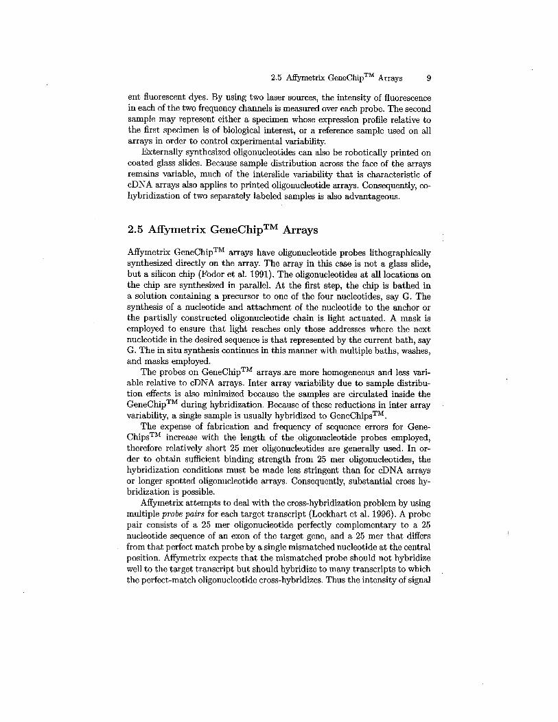
2.5 Affmetrix GeneChipTM Arrays

Affymetrix GeneChip ™ arrays have oligonucleotide probes lithographicallysynthesized directly on the array. The array in this case is not a glass slide,but a silcon chip (Fodor et al. 1991). The oligonucleotides at all locations onthe chip are synthesized in paralleL. At the first step, the chip is bathed in

a solution containing a precursor to one of the four nucleotides, say G. Thesynthesis of a nucleotide and attachment of the nucleotide to the anchor orthe partially constructed oligonucleotide chain is light actuated. A mask isemployed to ensure that light reaches only those addresses where the nextnucleotide in the desired sequence is that represented by the current bath, say

G. The in situ synthesis continues in this manner with multiple baths, washes,and masks employed.

The probes on GeneChipTM arrays.are more homogeneous and less vari-able relative to cDNA arrays. Inter array variabilty due to sample distribu-tion effects is also minimized because the samples are circulated inside theGeneChip ™ during hybridization. Because of these reductions in inter arrayvariabilty, a single sample is usually hybridized to GeneChipsTM.

The expense of fabrication and frequency of sequence errors for Gene-Chips ™ increase with the length of the oligonucleotide probes employed,

therefore relatively short 25 mer oligonucleotides are generally used. In or-der to obtain suffcient binding strength from 25 mer oligonucleotides, thehybridization conditions must be made less stringent than for cDNA arraysor longer spotted oligonucleotide arrays. Consequently, substantial cross hy-

bridization is possible.Affmetrix attempts to deal with the cross-hybridization problem by using

multiple probe pairs for each target transcript (Lockhart et al. 1996). A probepair consists of a 25 mer oligonucleotide perfectly complementary to a 25nucleotide sequence of an exon of the target gene, and a 25 mer that differsfrom that perfect match probe by a single mismatched nucleotide at the centralposition. Affymetrix expects that the mismatched probe should not hybridizewell to the target transcript but should hybridize to many transcripts to whichthe perfect-match oligonucleotide cross-hybridizes. Thus the intensity of signal


at the perfect match probe minus the intensity at the mismatched paired

probe may be a better estimate of the intensity due to hybridization to thetrue target transcript.

Current GeneChipsTM use 11 to16 probe pairs for each target gene butthe lengths of the probes are smaller than for cDNA arrays. The differences inperfect-match minus mismatch intensities are averaged across the probe pairsto give an estimate of intensity of hybridization to the target transcript; seeSection 4.3.

2.6 Other Microarray Platforms

Several companies such as Protogene (Menlo Park, CA) and Agilent Technolo-gies (Palo Alto, CA) in collaboration with Rosetta Inpharmatics (Kirkland,WA) have developed methods of in situ synthesis of oligonucleotides on glassarrays using ink-jet technology that does not require photolithography. Theink-jet technology of Agilent can also be used to attach pre synthesized DNAprobes to glass slides.

Another class of DNA microarrays utilzes cDNA probes printed on anylon membrane, and radioactive labeling of the sample. The radioactive labelprovides a stronger signal than fluorescent dye. This is useful when the amountof mRNA available for labeling is limited, but the wide scattering of labellimits the density of probes that can be printed on the array, and larger formatarrays are necessary. Although most of the principles of experimental designand analysis apply equally to arrays using radioactively labeled samples as toarrays using fluorescent labels, we generally talk in terms of the latter.

3

Design of DNA Microarray Experiments

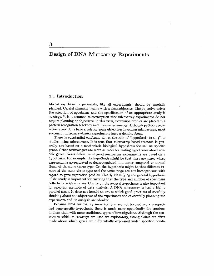
3.1 Introduction

Microarray based experiments, like all experiments, should be carefullyplanned. Careful planning begins with a clear objective. The objective drivesthe selection of specime~s and the specification of an appropriate analysisstrategy. It is a common misconception that microarray experiments do notrequire planning or objectives; in this view, expression profies are placed in apattern recognition blackbox and discoveries emerge. Although pattern recog-nition algorithms have a role for some objectives involving microarrays, mostsuccessful microarray-based experiments have a definite focus.

There is substantial confion about the role of "hypothesis testing" instudies using microarrays. It is true that micro array-based research is gen-erally not based on a mechanistic biological hypothesis focused on specific

genes. Other technologies are more suitable for testing hypotheses about spe-cifc genes. Nevertheless, most good microarray experiments are based on ahypothesis. For example, the hypothesis might be that there are genes whoseexpression is up-regulated or down-regulated in a tumor compared to normaltissue of the same tissue type. Or, the hypothesis might be that different tu-mors of the same tissue type and the same stage are not homogeneous withregard to gene expression profiles. Clearly identifyng the general hypothesisof the study is important for ensuring that the type and number of specimenscollected are appropriate. Clarity on the general hypotheses is also importantfor selecting methods of data analysis. A DNA microarray is just a highlyparallel assay. It does not herald an era in which good practices of carefullythinking about the objectives of the experiment and of carefully planning theexperiment and its analysis are obsolete.

Because DNA micro array investigations are not focused on a prespeci-

fied gene-specific hypothesis, there is much more opportunity for spuriousfindings than with more traditional types of investigations. Although the con-texts in which micro arrays are used are exploratory, strong claims are often

made about which genes are differentially expressed under specifed condi-

12 3 Design of DNA Microarray Experiments

tions, which are disreguated in diseased tissue, and which are predictive ofresponse to treatment. The serious multiplicity problems inherent in examin-ing expression profiles of tens of thousands of genes mandate careful planningand special forms of analysis in order to avoid being swamped by spuriousassociations .

Design issues can be divided into those relating to the design of the DNAmicro array assay itself and issues involving the selection, labeling, and ar-raying of the specimens to be assayed. In this chapter, we focus on the latterissues. Section 3.2 describes the importance of defining the study objectives fordesigning a microarray study, Section 3.3 discusses the diffculties in satisfyingstudy objectives when only two RNA samples are compared. The sources ofvariation and the levels of replication of the experiment, discussed in Section3.4, are important to consider when designing a study. Section 3.5 discusses

the possibilty of pooling samples and assaying the pooled sample with amicroarray. With dual-label microarrays, the different ways of pairing andlabeling the samples are discussed in Sections 3.6 and 3.7, respectively. Thechapter ends with a discussion of the sample sizes required to meet the studyobjectives.

3.2 Study Objectives

DNA microarrays are useful in a wide variety of investigations with a widevariety of objectives. Many of these 'objectives fall into the following categories.

3.2.1 Class Comparison

Class comparison focuses on determiing whether gene expression profiles dif-fer among samples selected from predefined classes and identifying which genesare differentially expressed among the classes. For example, the classes mayrepresent different tissue types, the same tissue under different experimentalconditions, or the same tissue type for different classes of individuals. In can-cer studies, the classes often represent distinct categories of tumors diferingwith regard to stage, primary site, genetic mutations present, or with regardto response to therapy; the specimens may represent tissue taken before or af-ter treatment or experimental intervention. There are many study objectivesthat can be identified as class comparison. The defining characteristic of classcomparison is that the classes are predefined independently of the expressionprofiles. Many studies are performed to compare gene expression for severaltypes of class definition. For example, two genotypes of mice may be stud-ied under two different experimental conditions. One analysis may addressdifferences in gene expression for the two types of animals under the sameexperimental condition and the other analysis may address the effect of theexperimental intervention on gene expression for a given genotype.

3.3 Comparing Two RNA Samples 13

3.2.2 Class Prediction

Class prediction is similar to class comparison except that the emphasis is ondeveloping a statistical model that can predict to which class a new specimenbelongs based on its expression profile. This usually requires identifyng whichgenes are informative for distinguishing the predefined classes, using thesegenes to develop a statistical prediction model, and estimating the accuracy ofthe predictor. Class prediction is important for medical problems of diagnosticclassification, prognostic prediction, and treatment selection.

3.2.3 Class Discovery

Another type of microarray study involves the identification of novel sub-types of specimens within a population. This objective is based on the ideathat important biological differences among specimens that are clinically andmorphologically similar may be discernible at the molecular leveL. For exam-

ple, many microarray studies in cancer have the objective of developing ataxonomy of cancers that originate in a given organ site in order to identifysubclasses of tumors that are biologically homogeneous and whose expressionprofiles either reflect different cells of origin or other differences in diseasepathogenesis (Alizadeh et al. 2000; Bittner et al. 2000). These studies mayuncover biological features of the disease that pave the way for developmentof improved treatments by identification of molecular targets for therapy.

3.2.4 Pathway Analysis

The objective of some studies is the identification of genes that are coregulatedor which occur in the same biochemical pathway. One widely noted example isthe identification of cell cycle genes in yeast (Spellman et aL. 1998). Pathwayanalysis is often based on performing an experimental intervention and com-paring expression profiles of specimens collected before and at various timeintervals after the experimental intervention. In some cases, however, pathwayanalysis may involve comparing the wild type organim to genetically alteredvariants.

3.3 Comparing Two RNA Samples

The initial cDNA microarray studies involved the cohybridization of onemRNA sample labeled with one fluorescent dye and a second mRA sam-ple labeled with a second fluorescent dye on a single microarray (DeRisi et aL.1996). This type of study, and the high cost of microarrays, left many investi-gators hoping and believing that no replication was needed. It also led to thepublication of a variety of statistical methods for comparing the expressionlevels in the two channels at each gene on a single microarray. Even today,


Affmetrix software is designed to compare gene expression on just two arrays(one sample on each array) and to compare two classes of specimens one mustcompare the specimens two at a time (Affetrix 2002).

The main problems with drawing conclusions based on comparing twoRNA samples apply to both dual-label and Affmetrix arrays. First, the rela-tive intensity for a given gene in the two specimens can reflect an experimentalartifact in tissue handling, cell culture conditions, RNA extraction, labeling,or hybridization to the arrays that is not removed by the normalization pro-cess. The analysis of two RNA samples each arrayed once provides very littleevidence that if the same two samples were rearrayed the results would besimilar.

Even more important, the conclusions derived from comparing two RNAsamples, even if they are arrayed on replicate arrays, apply only to thosetwo samples and not to the tissues or experimental conditions from whichthey were derived. For example, in comparing two RNA samples, none ofthe biological variabilty is represented. In comparing expression profiles of

tumors of one type to tumors of another type, there is generally substantialvariation among tumors of the same class (e.g., Hedenfalk et aL. 2001). Theremay even be substantial variation in expression within a single tumor. Hence,comparison of one RNA sample from one tumor of the fist type to one RNAsample from one tumor of the second type is not adequate. In comparingtissue from inbred strains of mice, the biological variabilty is generally lessthan for human tissue but some biological replication is stil necessary. Even

. for comparing expression of a cell line under two conditions, there is biologicalvariabilty resulting from variation in experimental conditions, growth andharvest of the cells, and extraction of the RNA. Hence some replication of theentire experiment is important. This is discussed further in the next section. \

3.4 Sources of Variation and Levels of Replication

Some important sources of variation in microarray studies can be categorizedas

. between individuals within the same "class" or between complete replica-

tion of tissue culture experiments under the same experimental conditions;. between specimens from the same individual or same experiment;

. between RNA samples from the same specimen;

. between arrays for the same RNA sample;

. between replicate spots on the same array.

Replicate arrays made from the same sample of RNA are often calledtechnical replicates, in contrast to biological replicates made from RNA frombiologically independent samples (Yang and Speed 2002b). There are, how-ever, several levels of biological replicates.

3.4 Sources of Variation and Levels of Replication 15

Suppose we wish to determine gene expression diferences between breasttumors with a mutated BRCAI gene and tumors without a mutation. If weperformed array experiments on one breast tumor with a BRCAI mutationand one without a mutation we would not be able to draw any valid conclu-sions about the relationship of BRCAI mutations to gene expression becausewe have no information about the natural variation within the two popu-lations being studied. The situation would not improve even if the tumorsunder investigation were large enough for us to be able to perform multiplemRN A extractions and run independent array hybridizations on each extrac-tion. Sets of tumors representative of the BRCAI mutated population andthe non-BRCAI mutated population are necessary to draw valid conclusionsabout the relationship of BRCAI mutations to gene expression. .

There is sometimes confusion with regard to the level of replication appro-priate for micro array studies. For example, in comparing expression profilesof BRCAI mutated tumors to expression profies of non-BRCAlmutated tu-mors, it is not necessary to have replicate arrays of a single RNA sampleextracted from a single biopsy of a single tumor. Having such replication mayprovide protection from having to exclude the tumor if the one array avaableis of poor quality, but such replications are merely assay replicates and do notsatisfy the crucial need for studying multiple tumors of each type. Often thebiological vaiation between individuals will be much larger than the assayvariation and it will be ineffcient to perform replicate arrays using specimensfrom a small number of individuals rather than performing single arrays usinga larger number of individuals.

In comparing expression profiles between two cell lines, or for a given cellline under different conditions, the concept of "individual" may be unclear.Suppose, for example, we wish to compare the expression profie of a cell linebefore treatment to the expression profie after treatment. Cell lines change

their expression profiles depending on the culture conditions. Growing thecells and harvesting the RNA under "fied conditions" wil result in variableexpression profiles because of differences in important factors such as the con-fluence state of the culture at the time of cell harvesting. Consequently, it isimportant to have independent biological replicates of the complete experi-ment under each of the conditions being compared. The degree of variationbetween independent biological samples may be less for experiments involvingcell lines or inbred strains of model species compared to those involving hu-man tissue samples, and this wil influence the number of biological samplesrequired as described in Section 3.8.

In some cases it is n8eful to obtain two specimens from the same individual.For example, if you are attempting to discover a new taxonomy of a diseasebased on an expression profie, it is useful to establish that the classificationis robust to sampling variation within the same individuaL. For many studiesof human tissue, however, the tissue samples will not be large enough toprovide multiple specimens for independent processing. It is important to

note that there is a distinction between multiple specimens from the same

,16 3 Design of DNA Microarray Experiments

individual and multiple independently labeled aliquots of one RNA sample.The latter wil show less variabilty than the former, especially when the tissue

is heterogeneous. However, even without tissue heterogeneity, variation maybe observed among expression profiles of multiple specimens taken from thesame individual because of differences in tissue handling and RNA extraction.

Performing technical replicate arrays with independently labeled aliquotsof the same RN A provides information about the reproducibilty of the mi-croarray assay, that is, the reproducibilty of tlie labeling, hybridization, andquantification procedures. It is useful to know that the reagents, protocolsand procedures used provide reproducible results on aliquots of the sameRNA sample. Generally, it wil be suffcient to obtain such technical repli-cates on just a few RNA samples. Serious attention should be devoted toreduce techncal variabilty in a study. If possible, RNA extraction, labeling,and hybridization of all arrays in an experiment should be performed by thesame individual using the same reagents. If spotted arrays are used, it is de-sirable to use arrays from the same print set and certaiy the same batchof internal reference RNA. If samples become avalable at different times ina long-term study, it is best to save frozen specimens so that all of the arrayassays can be done at approximately the same time.

When techncal replicate arrays of the same RNA samples are obtained,they can be averaged to improve precision of the estimate of the expressionprofie for a iiven RNA sample. If reproducibilty is poor, however, it maybe preferable to discard techncally inferior arrays rather than average repli-cates. Although averaging of replicates may seem ad hoc, analysis of variancemethods also average replicates although they account for the differences inprecision available for different samples based on their possibly varying num-ber of replicates. Replicate arrays of the same RNA samples are also sometimesused in dye-swap experimental designs described later in this chapter.

3.5 Pooling öf Samples

Some investigators pool samples in the hope that through pooling they canreduce the number of microarrays needed. For example, in comparing twotissue types, a pool of one type of tissue is compared to a pool of the othertissue type. Replicate arrays might be performed on each pooled sample. Al-though the pooled sample approach may be applicable for preliminary screen-ing, the approach does not provide a valid basis for biological conclusionsabout the types of tissues being compared. If only one array of each pooled

sample is prepared, then even the two pools cannot be validly statisticallycompared because there is no estimate of the variabilty associated with inde-pendently labeling and hybridizing the same pool onto different arrays. Evenif the two pools are hybridized to replicate arrays, one cannot assess the vari-ability among pools of the same type and so one doesn't know how adequate apool of that number of RNA specimens is in reflecting the population of that

3.6 Pairing Samples on Dual-Label Microarrays 17

tissue type. Unless multiple biologically independent pools (of distinct spec-imens) of each type are arrayed, only the pooled samples themselves can becompared, not the populations from which they were derived. Biological repli-cation is necessary. It can be achieved either by assaying individual samples,or by assaying independent pools of distinct samples. Studying independentpools of samples would be necessary in studying small model species where itmay be necessary to pool in order to obtain enough RNA for assay (Jin et al.2001).

3.6 Pairing Samples on Dual-Label Microarrays

With Affmetrix GeneChips TM, single samples are labeled and hybridizedto individual arrays. Spotted cDNA arrays, however, generally use a dual-label system in which two RNA samples are separately labeled, mied, andhybridized together to each array. When using dual-label arrays one mustdecide on a design for pairing and labeling samples.

3.6.1 The Reference Design

The most commonly used design, called the reference design, uses an aliquotof a reference RNA as one of the samples hybridized to each array. This servesas an internal standard so that the intensity of hybridization to a probe fora sample of interest is measured relative to the intensity of hybridization tothe same probe on the same array for the reference sample. This relative hy-bridization intensity produces a value that is standardized against variation insize and shape of corresponding spots on different arrays. Relative intensity isalso automatically standardized with regard to variation in sample distribu-tion across each array inasmuch as the two samples are mied and thereforedistributed similarly. The measure of relative hybridization generally used isthe logarithm of the ratio of intensities of the two labeled specimens at theprobe. Figure 3.1 is taken from Brody et al. (2002) who cohybridized labeledRNA from C2C12 myoblast cells and from lOTI/2 fibroblasts on an arraythat contained 100 spots for the glycerol-3-phosphate dehydrogenase gene.

The figure shows the vast range of intensities among spots printed with thesame clone on the same array. The ratio of intensities for the two samples,however, has little variation as evidenced by the tight linear association.

The reference design is ilustrated in Figure 3.2. Generally, the reference

is labeled with the same dye on each array. Any gene specific dye bias notremoved by normalization affects all arrays similarly and does not bias classcomparisons. Using a reference design, any subset of samples can be comparedto any other subset of samples. Hence the design is not dependent on thespecification of a single type of class comparison. For example, in studyingBRCAI mutated and BRCAI nonmutated tumors, one might be interested incomparing samples based on their mutation status, comparing samples based


6000 .5000 .

lõ .;.Q. 4000 . .(/ . .êi .nl .15 3000e.. øü:~ 2000 ,..I-0

1000

00 2000 4000 6000 8000 10000

Differentiated C2C12 cells (CY3J

Fig. 3.1. Intensities of labeled RNAfrom C2C12 myoblast cells and labeled RNAfrom 1OTI/2 fibroblasts hybridized to one array containing 100 spots of the glycerol-3-phosphate dehydrogenase gene. The figure shows the vat range of intensitiesamong spots printed with the same clone on the same array. The ratio of inten-sities for the two samples, however, has little variation. From Brody et aL (2002).

Rêfe;ren:ceDesiQ,n

Red

Grëen

Fig. 3.2. Reference design. Aliquot of reference sample is labeled with the same

label and used on each array.

3.6 Pairing Samples on Dua-Label Microarrays 19

on their estrogen receptor status, or comparing samples based on the stageof disease of the patient. The reference design is also convenient for class

discovery using cluster analysis because the relative expression measurementsare consistently measured with respect to the same reference sample.

If a laboratory uses reference designs with the same reference sample for allof their arrays, even those for different experiments, then all of their expres-sion profiles can be directly compared. Consequently, expression signatures ofdifferent tissues studied in different experiments can be compared. This lat-ter advatage can even extend to comparisons of expression profiles made bydiferent laboratories using reference designs with the same reference sample.

There is sometimes confusion about the role of the reference sample. Someinvestigators erroneously believe that analysis is always based on combiningsingle array determinations of whether the Cy5 (red) label is differentiallyexpressed compared to the Cy3 (green) label for a given spot on a given array.Therefore they assume that the reference sample must be biologically relevantfor comparison to the nOlleference samples. In fact, the reference sample doesnot need to have any biological relevance. The analysis will usually involvequantitative comparisons of the average logarithm of intensity ratios for oneset of arrays to average log ratios for another set' of arrays.

It is desirable that most of the genes be expressed in the reference samplebut not expressed at so high a level as to saturate the intensity detectionsystem. Often, the reference sample consists of a mixure of cell lines so thatnearly all genes will be expressed to some leveL. It is also important that a

single batch of reference RN A is used for all arrays in a reference design. Dif-ferent batches of reference RNA may have quite different expression profiles.When assaying samples collected over a long period of time, it is generallybest to freeze the RNA samples and to perform the microarray assays at onetime when all reagents can be standardized.

3.6.2 The Balanced Block Design

A disadvantage of the reference design is that half of the hybridizations areused for the reference sample, which may be of no real interest. Balanced blockdesigns (Dobbin and Simon 2002) are alternatives that can be used in simplesituations. For example, suppose one wished to compare BRCAI mutatedbreast tumors to BRCAI nonmutated breast tumors, that equal numbers ofeach tumor were available and that no other comparisons or other analyseswere of interest. One could hybridize on each array one BRCAI mutatedtumor sample with one nonmutated sample. On half of the arrays the BRCAImutated tumors should be labeled with the red dye and on the other half thenonmutated tumors should be labeled with the red dye. This block design isilustrated in Figure 3.3. The analysis of data for the block design is discussed

in Section 7.9. In its simplest form, a paired value t-test or Wilcoxon signed-rank test is performed for each gene, pairing the samples cohybridized to thesame array. The block design can accommodate n samples of each type using


ß.alancedBlo;ckDesign

Roo

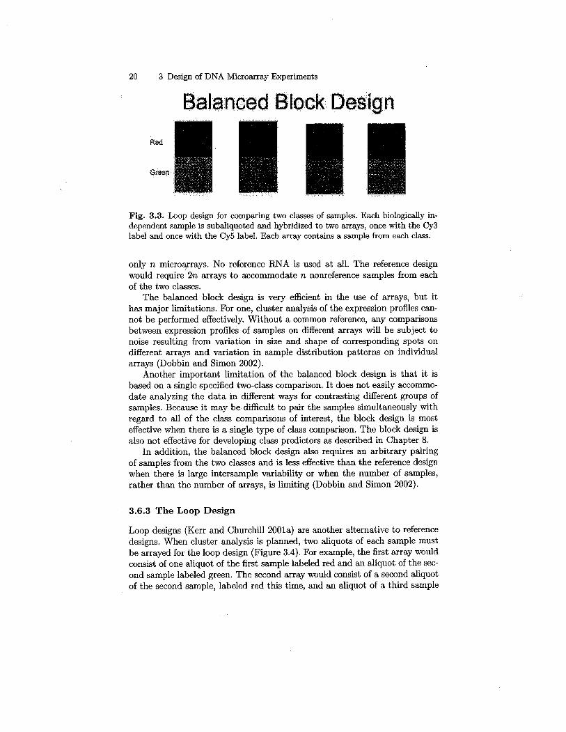
Fig. 3.3. Loop design for comparing two classes of samples. Each biologically in-dependent sample is subaliquoted and hybridized to two arrays, once with the Cy3label and once with the Cy5 labeL. Each array contains a sample from each class.

only n microarrays. No reference RNA is used at all. The reference designwould require' 2n arrays to accommodate n nOlleference samples from eachof the two classes.

The balanced block design is very effcient in the use of arrays, but ithas major limitations. For one, cluster analysis of the expression profiles can-not be performed effectively. Without a common reference, any comparisonsbetween expression profiles of samples on different arrays will be subject tonoise resulting from variation in size and shape of corresponding spots ondifferent arrays and variation in sample distribution patterns on individualarrays (Dobbin and Simon 2002).

Another important limitation of the balanced block design is that it isbased on a single specified two-class comparison. It does not easily accommo-date analyzing the data in different ways for contrasting different groups ofsamples. Because it may be diffcult to pair the samples simultaneously withregard to all of the class comparisons of interest, the block design is most

effective when there is a single type of class comparison. The block design isalso not effective for developing class predictors as described in Chapter 8.

In addition, the balanced block design also requires an arbitrary pairingof samples from the two classes and is less effective than the reference designwhen there is large inters ample variabilty or when the number of samples,rather than the number of arrays, is limiting (Dobbin and Simon 2002).

3.6.3 The Loop Design

Loop designs (Kerr and Churchil 2001a) are another alternative to referencedesigns. When cluster analysis is planned, two aliquots of each sample mustbe arrayed for the loop design (Figure 3.4). For example, the first array wouldconsist of one aliquot of the first sample labeled red and an aliquot of the sec-ond sample labeled green. The second array would consist of a second aliquotof the second sample, labeled red this time, and an aliquot of a third sample

3.7 Reverse Labeling (Dye Swap) 21

LQO'pDeslgn

r..M

Green

Fig. 3.4. Balanced block design for comparing two classes of samples. Each array

contains a biologically independent sample from eah class. Each class is labeled onhalf the arrays with one label and on the other half of the arrays with the otherlabeL Each biologically independent sample is hybridized to a single array.

labeled green. The third array would consist of a second aliquot of the thirdsample labeled red tils time, and an aliquot of a fourth sample labeled green.

This loop continues and concludes with the nth and final array which consistsof a second aliquot of the final sample n labeled red and hybridized with asecond aliquot of the first sample, labeled green this time. This uses n ar-rays to study n samples, using two aliquots of each sample. The loops permitall pairs of samples to be contrasted in a manner that controls for variationin spot size and sample distribution patterns using a statistical modeL. Con-

trasting two samples far apart in the loop, however, involves modeling manyindirect effects corresponding to the arrays linking the two arrays of interestand this adds substantial variance to many of these contrasts (Dobbin andSimon 2002). Consequently loop designs are not effective for cluster analysis.Loop designs can be used for class comparisons, but are less effcient than bal-anced block designs and require more complex methods of analysis than docommon reference designs. Loop designs are less robust against the presenceof bad quality arrays; two bad arrays break the loop. Loop designs also require

enough RNA to be available for each sample for at least two hybridizations.Because of these limitations, loop designs are not generally recommended.

3.7 Reverse Labeling (Dye Swap)

Some investigators believe that all arrays should be performed both forward-and reverse- labeled. That is, for an array with sample A labeled with Cy3and sample B labeled with Cy5, there should be another array with sample Alabeled with Cy5 and sample B labeled with Cy3. In general, tils is unneces-sary and wasteful of resources (Dobbin et aL. 2003a,b). Balanced labeling, as


described in Section 3.6.2 is in general much more effcient than replicatinghybridizations of the same specimens with swapped dye labeling. We discusshere, however, one circumstance where some reverse-labeling of samples isappropriate.

Dye swap or dye balance issues arise because the relative labeling inten-sity of the Cy3 and Cy5 may be different for different genes. Although thenormalization process may remove average dye bias, gene-specific dye biasmay remain. This is not important for comparing classes of nOlleference sam-ples using a reference design when the reference is consistently assigned thesame labeL. Suppose, however, that we wanted to compare tumor tissue to

matched normal tissue from the same patient Using dual-label microarrays.As discussed in Section 3.6.2, one effective design would be to pair tumor andnormal tissues from the same patient for co hybridization on the same array,with half of these arrays having the tumor labeled with Cy3 and the other halfhaving the tumor labeled with Cy5 (Figure 3.3). Because the dye a,signmentsare balanced, it is not necessary to perform any reverse-labeled replicate ar-rays of the tissues from the same patient (Dobbin et aL. 2003a,b). For a fiedtotal number of arrays, it is best to use the available arrays to assay tissuefrom new p~tients, using the balanced block design described, rather thanto perform replicate reverse-labeled arrays for single patients. The balancedblock design is also best when there are n tumor tissues and n normal tissueseven though the tissues are not from the same patients, or for comparing anytwo classes of samples. In these cases, the samples may be randomly paired,or paired based on balance with regard to potentially confounding variablessuch as the age of the specimens.

In some cases a reference design is used in which the primary objectiveis comparison of classes of the nOlleference samples but comparison to theinternal reference is a secondary objective. For example, there may be severaltypes of transgenic mouse breast tumors for comparison and the internal ref-erence may be a pool of normal mouse breast epithelium. Because the primaryinterest is comparison among multiple tumors models, a reference design maybe chosen. The use of a pool of normal breast epithelium as the internal refer-ence, rather than a mixture of cell lines, reflects some interest in comparisonof expression profiles in tumors relative to normal breast epithelium. Compar-ison to a pool of normal breast epithelium is somewhat problematic, however,for reasons described previously in Section 3.5. The conclusions derived fromcomparison of the tumor samples to the internal reference will apply to thatpool of normal epithelium, but it wil not be possible to evaluate how repre-

sentative that pool is. Nevertheless, the comparison may be of interest.In order to ensure that the comparison of tumor expression to that of the

reference is not distorted by gene-specific dye bias when using a referencedesign, some reverse-labeled arrays are needed. One can then fit a statisti-cal analysis of variance model to the logarithms of the intensities for eachchannel as described in Section 7.9. Not all arrays need to be reverse-labeled;5 tolO reverse-labeled pairs of arrays will generally be adequate. Except for

3.8 Number of Biological Replicates Needed 23

this purpose of comparison of experimental samples to the common referencein a reference design, however, Dobbin et al. (2003a,b) recommend againstreverse-labeling of the same two RNA samples.

3.8 Number of Biological Replicates Needed

As indicated in Section 3.3, it is not generally meaningful to compare expres-sion profiles in two RNA samples withòut biological replication. The numberof independent biological samples needed depends on the objectives of the ex-periment. We describe here a relatively straightforward method for planningsample size for testing whether a particular gene is differentially expressedbetween two predefined classes. Such a test can be applied to each gene if weadjust for the number of comparisons involved (Simon et al. 2002).

This approach to sample size planning may be used for dual-label arraysusing reference designs or for single-label oligonucleotide arrays. For dual-label arrays the expression level for a gene is the log ratio of intensity relativeto the reference sample; for Affetrix GeneChip ™ arrays. it is usually thelog signal, discussed in Chapter 4. The approach to sample size planningdescribed here is based on the assumption that the expression measurementsare approximately normally distributed among samples of the same class. Letcy denote the standard deviation of the expression level for a gene amongsamples within the same class and suppose that the means of the two classesdiffer by 8 for that gene. For example, with base 2 logarithms, a value of8 = 1 corresponds to a twofold difference between classes. We assume thatthe two classes wil be compared with regard to the level of expression ofeach gene and that a statistically significant diference wil be declared ifthe null hypothesis can be rejected at a significance level a. The significancelevel is the probabilty of concluding that the gene is differentially expressedbetween the two classes when in fact the means are the same (8 = 0). Thesignificance level q will be set stringently in order to limit the number of falsepositive findings inasmuch as thousands of genes wil be analyzed. The desiredstatistical power wil be denoted 1 - ß. Statistical power is the probabilty ofobtaining statistical significance in comparing gene expression between thetwo classes when the true difference in mean expression levels between theclasses is 8. Statistical power is one minus the false negativity rate (ß).

Under these conditions, the total number of samples required from differentindividuals or different replications of the experiment approximately satisfiesthe equation:

4(ta/2 + tß)2n = (8jcy)2 '

where ta/2 and tß denote the (100)aj2 and 100ß percenties of the t distri-bution with n - 2 degree of freedom. Because the t percentiles depend on

n, however, the equation can only be solved iteratively. When the number of

(3.1)


samples n is sufciently large, Equation (3.1) can be adequately approximatedby

4(Za/2 + Zß)2n = (8/a)2 ' (3.2)where Za/2 and zß denote the corresponding percentiles of the standard nor-mal distribution (Desu et aL. 1990). The normal percentiles do not dependon n, and hence equation (3.2) can be solved directly for n. For example, fora = 0.001 and ß = 0.05 as recommended below, the standard normal per-

centiles are Za/2 = -3.29 and zß = -1.645, respectively. Expressions (3.1)

and (3.2) give the total number of biologically independent samples neededfor comparing the two classes; n/2 should be selected from each class.

The fact that expression levels for many genes will be examined indicatesthat the size of a should be much smaller than 0.05. The 0.05 value is onlyappropriate for experiments where the focus is on a single endpoint or sin-gle test. If a = 0.05 is used for testing the differential expression of 10,000

genes between two classes, then even if none of the genes is truly differentiallyexpressed, one would expect 500 false discoveries; that is, 500 false claims ofstatistical significance. The expected number of false discoveries is a times thenumber of genes that are nondifferentially expressed. This is true regardlessof the correlation pattern among the genes.

In order to.' keep the number of false discoveries manageable with thou-sands of genes analyzed, a = 0.001 is often appropriate. For example, usinga = 0.001 with 10,000 genes gives 10 expected false discoveries. This is muchless conservative than the multi-test adjustment procedures used for clinicaltrials where the probabilty of even one false discovery is limited to 5%. Werecommend ß = 0.05 in order to have good statistical power for identifynggenes that really are differentially expressed. If the ratio of sample sizes inthe two groups is k:l instead of 1:1, then the total sample size increases by afactor of (k + 1)2/4k compared to formula (3.2).

The parameter a can usually be estimated based on data showing the de-gree of variation of expression values among similar biological tissue samples.a wil vary among genes. For log ratio expression levels, we have seen themedian values of a of approximately 0.5 (using base 2 logarithms) for humantissue samples and similar values for Affetrix GeneChips TM. The parame-ter 8 represents the size of the difference between the two classes we wish to beable to detect. For log2 ratios or log2 signals, 8 = 1 is corresponds to a twofolddifference in expression level between classes. This value of 8 is reasonable be-cause differences of less than twofold are diffcult to measure reproducibiltywith microarrays. Using a = 0.001, ß = 0.05, 8 = 1 and a = 0.50 in (3.2)gives a required sample size of approximately 26 total samples, or 13 in eachof the two classes. The more accurate formula (3.1) gives a requirement of 30total samples, or 15 in each of the two classes.

The within-class variabilty depends somewhat on the type of specimens;human tissue samples have greater variabilty than inbred strains of IIce or

3.8 Number of Biological Replicates Needed 25

than cell lines. In experiments studying micro arrays of kidney tissue for inbredstrains of mice, the median standard deviation of log ratios for a normal kidneywas approxiately 0.25, with little variation among genes. For cell lie data

on Affmetrix GeneChips TM, we have seen similar standard deviations forlog2 signals. Using a = 0.001, ß = 0.05, 8 = 1 and (j = 0.25 in formula (3.1)gives a required sample size of 11 total samples. Because we cannot have 5.5samples per class, we should round up to 6 samples per class. If this werea time-series experiment with more than two time points, then one shouldplan for 6 animals per timepoint in order to enable expression profiles to becompared for all pairs of time points.

The discussion above applies either to dual-label arrays using a referencedesign and log ratio as the measure of relative expression, or to single-label ar-rays such as the Affmetrix GeneChipTM arrays using log transformed signalsor another measure of expression. When dual-label arrays are used with theblock design to compare either naturally paired or independent samples fromtwo classes, then the same formulas apply but the definition of (j changes.For the block design, (j represents the standard deviation of vaiation acrossarrays of the log ratio computed with one sample from each class (Dobbin etal. 2003). Preliminary data are generally needed to estimate (j.

Many of the considerations for comparing predefined classes also applyto identifying genes that are significantly associated with patient. outcome(Simon et al. 2002). When the outcome is survival and not all patients arefollowed until death, the analogue of expression (3.2) is

E = (Za/2 + Zß)2(Tln(8))2

(3.3)

E denotes the number of events (e.g., deaths) that need to be observed inorder to achieve the targeted statistical power. For survival comparisons, thestatistical power often depends on the number of events, rather than the num-ber of patients. For a given number of patients accrued, the number of eventswil increase as the duration of followup increases. There is a tradeoff betweennumber of patients accrued and duration of followup in order to achieve atargeted number of events. In expression (3.3), T denotes the standard devia-tion of the log ratio or log signal for the gene over the entire set of samples. 8represents the hazard ratio associated with a one-unit change in the log ratioor log signal and In denotes the natural logarithm. Note that we are assumgthat the log ratio or log signal values are based on logarithms to the base 2,so a one-unit change in the expression level represents a twofold change.

If T = 0.5 and 8 = 2, then 203 events are required for a two-sided signifi-cance level of 0.001 and power of 0.95. This makes for a large study in mostcases because to observe 203 events in a group of patients with a 50% eventrate requires 406 patients. The large number of events results from assumingthat a doubling of hazard rate requires a two standard deviation change in logratio. Hence most patients would have expression levels that had very limtedeffects on survivaL. Therefore it may be more reasonable to size the study for


detecting statistically significant differences in only the more variable genes,for example, T = 1 and 8 = 2, which results in 51 required events. Genes thathave small standard deviations across the entire set of samples are diffcult touse for prognostic prediction in clinical situations.

The multivariate permutation tests described in Chapter 7 are a morepowerful method for finding differentially expressed genes than the univariateparametric test that is the basis for formulas (3.1) and (3.2). Nevertheless,

the sample size formulas given here are useful for planng purposes and pro-vide control of the number of false discoveries in a reasonable manner. Othermethods have been described by Black and Doerge (2002), Lee and Whit-more, (2002), and Pan et aL. (2002). Adequate methods for determining thenumber of samples required for gene expression studies whose objectives areclass prediction or class discovery have not yet been developed. Hwang et aL.

(2002) provide a method of planning sample size to test the hypothesis thatthe classes are completely equivalent with regard to expression profile. Thesample size formulas given above provide reasonable minimum sample sizesfor class prediction studies. Often, however, developing multivaiate class pre-dictors or survival predictors involves extensive analyses beyond determiningthe genes that are informative univariately. Consequently, larger sample sizes

are generally needed for class prediction studies (Rosenwald et aL. 2002).In class prediction studies it is important to estimate the misclassification

rate of the identified multivariate predictor. There is a problem using the samedata to develop a prediction model and to estimate the accuracy of the model,particularly when the number of candidate predictors is orders of magnitudelarger than the number of cases (Simon et aL. 2003). Consequently, special

methods of analysis must be used to provide unbiased estimates of predic-tion accuracy. One approach is to split the data into a training set and avalidation set (Rosenwald et aL. 2002). Other approaches involve more sophis-ticated methods such as cross-validation or bootstrap resampling (discussed inChapter 8). Cross-validation and bootstrap resampling can be used when thederivation of the prediction rule can be clearly defined as an algorithm withno subjective elements. In many cases, the derivation of the prediction rule ismore complex and involves numerous analyses that cannot be easily specifiedin a manner that can automatically be applied to resampled datasets. In thesecases, it is necessary to use the split sample approach to obtain an unbiasedestimate of the accuracy of the class prediction rule. Initially the data aredivided into a training set and a validation set. This division may be donerandomly or may be balanced by factors such as an institution contributingthe specimens. The validation set is put aside and not analyzed at all untila completely specified prediction rule is defined based on analyses conductedusing the training set. The prediction rule resulting from the analysis shouldbe completely specified, including the estimation of parameters and the es-tablishment of threshold values for class prediction. After the analysis of thetraining set is completed, the validation set is unocked and the completelyspecified prediction rule is applied to the cases in the validation set. The pre-

3.8 Number of Biologica Replicates Needed 27

diction accuracy is determined based on the performance of the predictor onthe validation set. Usually about one third to one half of the total dataset isreserved for the validation set. Therefore in planing the size of a class pre-diction study that will use the split sample approaèh, it should be recognizedthat perhaps only half of the data will be available for development of the

multivariate predictor.Often investigators use validation sets that are far too small to provide

meaningful validation. Table 3.1 shows the upper 95% confidence limit for themisclassIfcation rate as a function of the observed proportion of misclassifiedspecimens and the number of specimens in the validation set. Suppose thatthe true misclassification rate is 10% and you are lucky enough to observeno misclassifications in the validation set. With only 10 specimens in thevalidation set you would be able to bound the true misclassification rate tobe no greater than 26%. But it is just as likely that you would obtain 20%of the validation set misclassified. In this case, even with 50 samples in thevalidation set, you would only be able to bound the true misclassification rateto be no greater than 32%. Consequently, a substantial validation set is neededin order to adequately estimate the true misclassification rate.

Table 3.1.

Number of Upper 95% Confidence Liuut for Misclassification RateValidation Samples

None Misclassified inI 20% Misclassified inValidation Set (%) Validation Set (%)

5 45 66

10 26 51

20 14 40

50 6 32

4

Image Analysis

After hybridization of fluorescently labeled cDNA molecules to the microar-ray, the array is stimulated with a laser and the intensity of fluorescence is

measured at a dense grid of pixel locations on the array. An image file is cre-ated that stores all of the pixel-level intensities. There are many more pixelsthan probes on the array. Image analysis is the procedure by which pixel level

data are processed and converted to measures of intensity for the arrayedprobes. There are several image analysis methods available and it is useful forthe investigator to have some understanding of the approaches used.

We begin with a brief description of how images of gene expression arraysare created. Then we describe the main steps of image analysis: gridding, seg-mentation, background correction, feature (signal) intensity extraction, andflagging spots for exclusion. Because the methods used for cDNA microarraysand Affmetrix GeneChip ™ arrays are different, we discuss the above stepsfor the two types of arrays separately.

4. i Image Generation

A scanner (laser scanning confocal microscope) or a charge-coupled device

(CCD) camera is used to quantify the intensity of fluorescence at each pixellocation on the microarray. These intensities are saved in a file formatted asa 16 bit tagged image file (TIFF). The fluorescent dye molecules hybridized

to the probes emit photons when stimulated by a laser. Emission wavelengthsdiffer for the two dyes, thus the emitted photons can be selectively filteredto allow quantification of the amount emitted by each dye. For cDNA mi-croarrays, the dyes Cy3 and Cy5 have emission wavelengths in the 510 to 550nm and 630 to 660 nm ranges, respectively. With commonly used scanners,the emitted light is captured by a photomultiplier tube (PMT) detector inthe scanner and converted into electric current. The PMT's voltage can beadjusted in each channel to maxmize the dynamic range of the scanner withminimal saturation of pixels and also to get balanced intensities between the

30 4 Image Analysis

two channels. Pixels are saturated when more photons are detected than thePMT can process or when the output of the PMT exceeds the range of theanalogue-to-digital converter. Saturated pixels are displayed as white pixelsin the image. The differences in amplification resulting from PMT voltageadjustment will lead to changes in signal intensity, but this should not affectresults for the majority of genes (except for the saturated spots) after propernormalization (see Chapter 6). The intensity for each probe is proportional tothe number of molecules of the fluorescent label in DNA bound to the probe.

4.2 Image Analysis for cDNA Microarrays

4.2.1 Image Display

Figure 2.2 shows a typical cDNA microarray image. It has two rows and twocolumn of blocks called subgrids, which are uniformly spaced. Each subgridconsists of several rows and columns of spots. An enlarged image of one spotpatch is shown in Figure 4.1, and the smallest discernable element in that en-larged image is called a pixeL. The raw intensities for each of the two channelsare saved as 16 bit binary integers. They can be displayed as images with pixelvalues ranging from 0 to 65,535 shades of grey. The darkest black pixels rep-resent low-intensity vslue and the bright white pixels represent high-intensityvalue. For purposes of visual display, the two separate 16 bit TIFF fies arefrequently combined and saved as a 24 bit composite RGB (red-green-blue)image. In this RGB composite, each of the three color channels is composedof only an 8 bit image. In order to be displayed as a 24 bit composite RGBoverlay image, the raw images must first be reduced from 16 bits to 8 bitsusing an image compression method. Then the image from Cy3 is placed inthe green channel, the image from Cy5 is placed in the red channel, and theblue channel is set to O. For image analysis the original 16 bit TIFF files areused.

4.2.2 Gridding

The first step in array image analysis is to overlay a rectangular grid onto thepixels in a manner that isolates each spot within a cell. Gridding is usually asemi or fully automated process that takes advantage of the fact that roboticspotting is performed in a regular predetermined manner. Most software sys-tems begin by estimating the overall position of the array in the image, theseparation between rows and columns of grids, the spacing of spots within eachgrid, and translation of individual grids or spots. For example, GenePix (Axon2001) automatically generates grids using tlie printing information (grid con-figuration), and then provides a manual fine-tuning option.

4.2 Image Analysis for cDNA Microarrays 31

4.2.3 Segmentation

Gridding establishes the location of a rectangular patch that contains the spot.The second step, segmentation, involves identifying the pixels within the patchthat are contained in the spot. Thi set of pixels is called the foreground region

or spot mask. Several different segmentation algorithms are in common usefor this purpose.

Fixed or adaptive circle segmentation is based on approximating the fore-ground region by a circle. Fixed circle segmentation uses the same circle di-ameter for all spots. Adaptive circle segmentation uses the intensity data toestimate the best diameter separately for each spot. However, both approachesare of limited accuracy inasmuch as real spots have irregular shapes (Figure4.1) because of printing, hybridization, and slide surface chemistry factors.

Fig. 4.1. An enlarged spot patch shown at pixel leveL. The spot is noncircularshaped, with a circular mask placed for segmentation.

To address the problems caused by spot irregularities, adaptive segmenta-tion methods such as watershed and seeded region growing have been applied(Beucher and Meyer 1993; Adams and Bischof 1994). The watershed algo-rithm is applied separately to each spot patch. The pixels in a spot patch arepartitioned into disjoint watershed sets. All the pixels in the same watershedset "drain" into the same local mjnimum with regard to the distribution ofpixel intensities. The definition of watersheds is as follows. For each point inthe spot patch, a path is determined by choosing the direction of the steep-est descent with respect to intensity. These paths lead to local minima. Allpixels that have a path leading to the same minimum belong to the samecatchment basin and together constitute one segment. The borders betweentouching segments are the watersheds. The average intensity in each segment

32 4 Image Analysis

is computed, and the segments with largest average intensities are taken asthe foreground region. This region need not be contiguous or regular.

The seeded region growing (SRG) algorithm is another method for repre-senting irregular foreground regions. SRG is based on choosing a small numberof high-intensity pixels as the initial seeds. The region defined by each seed isenlarged contiguously to contain other relatively high-intensity pixels. Whena region cannot be further enlarged without introducing pixels with intensitybelow some specified threshold criterion, growth of that segment ceases. Theresulting segments of high-intensity pixels are taken as the foreground region.

Histogram segmentation is another commonly used method. It does notrely on spatial information. Instead, the histogram of intensities for pixelswithin each spot patch is computed. Threshold percentiles are then used todefine the foreground and background regions; for example, pixels in the 5thto 20th percentiles of the intensity ditribution are often chosen for the back-ground, and pixels in the 80th to 95th percentiles are chosen for the fore-ground. A non-spatial segmentation method based on the Mann-Whitney testhas also been proposed (Chen et al. 1997).

4.2.4 Foreground Intensity Extraction

Once the foreground and background regions are determined for each spot,the pixel values are summarized to give a single measurement for each region.Common summary values for the foreground include the mean or medianvalue of the pixel intensities. The mean pixel intensity has the appeal of beingdirectly related to the total (sum) of pixel intensities in the foreground. If

spots are irregularly shaped and fixed or adaptive circle segmentation is used,the foreground region could include pixels not part of the probe leading to anunderestimate of the true foreground intensity. However, this downward biasis corrected when the ratio of the two channel background-adjusted intensitiesis calculated.

Occasionally, spots contain a few aberrantly high pixel intensities due toartifacts and these may tend to distort the mean value. For this reason, someinvestigators prefer to sumarize the foreground pixels by the median pixelintensity. Although more robust to aberrant pixels, the median has the dis-advantage of not being directly related to the total intensity. Also, if spotsare very elongated ovals or have large "holes" covering more than 50% of thepixels in the circular mask applied in fied or adaptive circle segmentation,the median value may be equal to background intensity, totally missing thesignaL. The trimmed mean may be a better alternative than the median. A k%trimmed mean is the mean calculated after excluding the largest (or smallest)k percentage of the pixel intensity values.

Methods that allow flexibilty in spot shape such as histogram or adaptivemethods have the potential of better estimating total intensity of bound labeL.Nevertheless, calculating the mean foreground with fied or adaptive circles isrelatively simple and seems to work well ,in practice. Comparisons performed

4.2 Image Analysis for cDNA Microarrays 33

by Yang et aL. (2002c) indicated that the differences among the algorithmhad very small impact on foreground intensity values.

4.2.5 Background Correction

Considering nonspecific binding and auto-fluorescence, it seems clear that theforeground intensity would be more properly proportional to abundance ofbound labeled cDNA if an accurate adjustment for background fluorescencecould be performed. Currently, there are different approaches to backgroundadjustment, and studies have shown that the choice of background adjustmentmethod can have a large impact on the final output such as log ratios (Yanget al. 2002c; Jain et al. 2002).

Global background correction uses the same constant to represent thebackground for all spots. This constant can be calculated by using a set ofnegative control spots. Alternatively, one can use a low percentile (e.g. thirdpercentile) of all the pixel intensities as the background leveL. Brown et al.(2001) computed a global background estimate as part of their normalizationprocedure to make the average ratio across the array as close to one as possible.However, global estimation does not take into account the local backgroundvariations that exist in many cases.

Regional background correction provides greater flexibilty than global cor-rection (Axon 2001; Yang et aL. 2001; Jain et aL. 2002). For example, thealgorithm used by GenePix is based on a circle centered on each spot. Theregion from which the background is calculated for any spot has a diameterthat is three times the diameter of the circle used to defie the foregroundfor that spot. Pixels contained within the large circle that are not within anyforeground region and are not wholly inside a two-pixel wide ring around theforeground circle of the current spot are used to compute the background forthe current spot.

Yang et aL. (2001) applied an algorithm called morphological opening

(Soile 1999) for background adjustment. Morphological opening is a methodfor obtaining a regionally smoothed estimate of the background for each spotwithout having to. estimate the boundaries of the foreground regions of thespots. The algorithm is based on virtually moving a square structural element(SE) over the face of the array. The stfuctural element is a window that ismuch larger than the size of any spot, but smaller than a grid of spots. Whenthe SE is centered on a particular pixel, the intensity of that pixel is replacedby the minimum intensity of pixels covered by the SE. This is called the "ero-sion" step. After the erosion step is completed, the SE is again virtually movedover the face,:of.:the array in a "dilation" step. When the SE is centered ona pixel, the intenSity of that pixel is replaced by the maximum of the valuescreated during erosion for the pixels covered by the SE. The morphologicalopening fiter removes all features that are not big enough to contain the struc-ture element. By choosing a square structuring element much larger than thespot size, the operation removes all the spots and generates an image as an

34 4 Image Analysis

estimate of the background for the entire slide. Background for each spot isthen calculated by sampling the estimated background image at the nominalcenters of the spots. Compared with other background correction methods,morphological opening showed a low withIn- and between-slide variabilty inratios in the study by Yang et al. (2002c), but there was no gold standard bywhich to evaluate whether the resulting estimates were more accurate.

Local background estimation may provide a poor estimate of nonspecificfluorescence because it may be highly variable if it is based on too small aregion. Consequently, it is not uncommon for spots to have higher values forthe background than for the foreground. Log ratios of background-adjustedsignal values in the two channels are imprecise estimates of relative abundanceof transcripts in the two samples for probes in which both of the backgroundadjusted signals are extremely low. It may be better to exclude such probesfrom subsequent analysis. This is discussed further in Chapter 5.

4.2.6 Image Output File

For each spot and channel, the output file sumarizes quantities such as fore-ground mean, median, and standard deviation of pixel intensities; backgroundmean, median and standard deviation of pixel intensities; and the number ofpixels in the foreground and background. The log bas 2 ratio for each spotis: FR-BR

10g2 FG - BG' (4.1)

where F R and FG denote the foreground mean or median intensities of thered and green chanels, and BR and BG denote the corresponding back-ground mean or median intensities. Mean foreground intensities and medianbackground intensities are recommended in most cases. The log ratio esti-mates the relative abundance of the corresponding gene trancripts in the two

samples that were cohybridized. to the array. Using the log ratio instead ofthe ratio makes the distribution more symmetrical and the vaiation less de-pendent on absolute signal magnitude. Most investigators use log ratios to dosubsequent analysis. However, some methods such as ANOVA methods workon the log signal directly rather than on log xatios (Kerr and Churchil 2001a;Wolfiger et al. 2001; Dobbin et aL. 2002, 2003).

Problematic spots should be flagged and omitted from the subsequent

analysis. Image analysis packages provide the abilty to flag individual spots

automaticaly and manualy, and flags are exported to the output file. Thosespots include the ones not at the expected location, ones with a negative redor green signal afer background subtraction, ones with too many saturatedpixels, and ones with no hybridization.

4.3 Image Analysis for Affetrix GeneChipTM 35

4.3 Image Analysis for Affmetrix GeneChipTM

GeneChipTM software analyzes the image data fie (.dat) and computes a sin-gle intensity value for each probe cell on the array. The intensity data aresaved to another fie (.cel). Figure 4.2 represents a feature-level view of ahigh-density Affymetrix GeneChipTM. Each gene has 16 to 20 probe pairs

Fig. 4.2. Feature view of Afetrix GeneChipTM.

that are scattered on the chip. Newer chips such as the Human Genome U133Set, the Rat Expression Set 230, and Mouse Expresion Set 430 have only11 probe pais per gene. For each probe pair, the upper perfect match (PM)probe usually gives a greater hybridization signal than its mismatch (MM)counterpart (Figue 4.3). However,' it is possible that the MM probe sequencehas high homology with another unown sequence. Consequently, the mis-

(

36 4 Image Analysis

match probe may have even a greater signal than the perfect match probe.Control probes located at the corners of the probe array are used to align agrid to delineate the probe cells.

..

Fig. 4.3. Enlarged view of Affetrix GeneChipTM. Probe pairs appear as two

bright stripes, with the upper stripe representing a perfect match (PM) probe andthe corresponding mismatch (MM) probe directly beneath. Each grid represents asmall region of the chip (typicaly 24 ¡im by 24 ¡im for thé high density arays and50 ¡im by 50 ¡iID for the low density arrays) containing 106 to 107 copies of a given

probe.

GeneChip ™ software defines a feature intensity as the 75th percentile ofthe pixel intensities for that feature afer removing the boundary pixels (Lock-hart et al. 1996). Sometimes the bright intensities tend to blur the PM/ MMboundar and result in an upwar bias for the MM intensity. Schadt et aL.(2001) proposed triming pixel intensities more than three standard devia-tions from the mean pixel value within a feature.

Background correction is also necessary for the GeneChip ™ arrays. A

high background implies that impurties, such as cell debri and salts, arebinding to the array in a nonspecific manner and that these substances arefluorescing at 570 DI (the scanng wavelength). The GeneChipTM softareuses a regionalized method to do background subtraction. The array is firstsplit into N rectanguar zones (default 16). Withi each zone, bacound in-tensities are calculated by averaging the lowest 2% of probe cell intensities, andbackground vaues are smoothed across the zones to obtain the cell-specificbackground estimates.

For the GeneChip ™ arrays, the average difference was the origial wayto produce gene-level sumaries:

1- ".(PMi-MMi),n~i (4.2)

where n represents the total number of probe pairs for the gene, and PMiand. MMi indicate the corresponding perfect match and mismatch probe in-tensities after bacground. correction for the ith probe pair for the gene. In

4.3 Image Analysis for Affetrix GeneChip ™ 37

contrast to the relative quantification of hybridization represented by cDNAarray-based ratios, the intensity vaues derived from GeneChipTM arrays areconsidered to measure absolute hybridization. Any hybridization to the MMprobe represents the level of nonspecific binding. Therefore it was thoughtthat the intensity measured from the MM probe could be used as an estimateof cross-hybridization.

Since the above average difference measure frequently produced negativevalues, AfetrIx modified the algorithm in its Microarray Suite User Guide

version 5. If the MM value is larger than the PM vaue for a probe pair, thenthe MM vaue is replaced by a smaller contrast vaue (CT). The CT value isbased either on the average ratio between PM and MM for all of the probepairs of that probe set, or (if that measure is too small) a value slightly smallerthan PM. If the MM vaue is smaller than the corresponding PM value,-thenthe CT value equals the MM value. The absolute expression value for probeset k is called the "signal log valui=" (SLV) and is defined as

..

SLVk = Biweighttlog2(PMi,k - CTi,k) : i = 1,... ,nH, (4.3)

where Biweight stands for the one-step Tuey biweightfuction operatingon the logs of the pairwie intensity differences between the PM and MMprobe pairs for all of the n probe pairs in probe set k. The Tuey biweightalgorithm (Hoaglin et al. 1983) is a method of robusly averagig values so asnot to be heavily afected by outliers. It uses the median to define the centerof the data. Then it uses the distance of each data point from the median todetermine how much each value should contribute to the average. The signalvalue reported by the MAS software is a normalzed signal and is describedin Chapter 6.

Alternative methods for estimating the probe set sumar signal are underactive investigation (Efron et al. 2001; Li and Wong 2001a; b; Naef et al. 2001,Irizarryet al. 2003). Efron et aL. (2001) proposed using parial MM values(half or one third) as rough estimates of cross-hybridization. A model-basedapproach for calculating gene sumaries from probe level data wa proposedby Li and Wong (200la, b). For each gene k, they model the average dierencesin probe pai i for array j as PM;j - MMij = OJlPi + êij. We have supreseduse of the subscript k for eas of notation but separate models are fit foreach gene k. The term OJ represents an average expreson index for the geneon array j, and the lPi terms represent probe-specific sensitivities for probe

pair i. The e term represent random experimental error. The probe-specific

sensitivities. are estimated using the data from all arrays in the experiment.These sensitivities indicate which probes of the probe set for gene k detectvariations acros the arrays and which do not. The array-specifc expression

index OJ for a given gene k is estimted as a weighted liear combination of thePM - MM diferences for that probe set, with the probe sensitivity estimatesbeing the weights. The Li and Wong method al provides confdence intervsfor the expression index of each gene on each array and these interv can be

38 4 Image Analysis

.

used for quality control puroses to distinguish the genes whose expression

index is well determined from those in which it is not.The issue of how to combine the PM and MM pairs to estimate an ex-

pression index for each gene on each array is stil under intensive academic

research. Some investigators even recommend using only the PM values andnot the MM values in estimating the expression indices (Naef et aL. 2001).

5

Quality Control

5.1 Introduction

Microaray signal intensities inherently contain a significant amount of noise.Usually the amount of noise in the signl is manageable and reliable conclu-sions can be made about the level of expression of a given probe. However, incertain cases there may be no reliable signal avalable or the noise dominatesthe signaL. In these cases, it is advisable to either replace these values with animputed value or else elinate the probe from the analysis. In tlus chapterwe discuss the circumstances under wluch an observation or set of observ-tions should be excluded as well as methods of imputing vaues for excludedobservations.

Determination of the acceptable amount of nois requires judgment onthe part of the investigator. Many of the quality control suggestions in tluschapter are of the form: Exclude a measured value should its quality fall belowa certain threshold. We provide gudelines as to what reasonable thresholdsmight be, but these should not be considered the only acceptable thresholds.

. If the use of a particular set of thresholds leads to an unacceptable numberof mising vaues, it might be reasonable to consider weakenig the quality

control standards. If, on the other hand, large numbers of outlier observtionsseem to be corrupting the analysis, it may be necessary J;o requie greaterstringency of quality control and raie the thresholds.

There are three levels at wluch qualty control may be warranted: the probelevel, the gene level and the array leveL. By poor probe quality, we mean poorquality of one particular gene expression measurement on one paricular array.By poor gene quality, we mean poor qualty of the expression measurementfor a sinle gene across all arrays. By poor array quality, we mean poor qualityof all spots on one particular glass slide or gene chp.

Sections 5.2 through 5.4 address quality control issues for two-color cDNAarrays. In section 5.5, we dicuss wluch of these issues apply to the qualitycontrol of Afetri data.

40 5 Quality Control

5.2 Probe-Level Quality Control for Two-Color Arrays

In the case of two-color cDNA arrays, the probes will be the individual spotsprinted on the slide. Poor quality at the spot level on a given array canoccur for a varety of reasons, some of which are technical such as a faulty

printing, uneven distribution of the sample on the slide, or contaminationwith debris. Other reasons are related to the size of the signal relative tothe noise. Because there are many ways in which a poorly measured spotcan occur, there are multiple methods of detecting poorly measured spots.We recommend considering all of the following criteria, and eliminating orimputing any spot that fails any of them.

5.2.1 Visual Inspection of the Image File

Sometimes it is possible to notice anomalies on a slide by visually inspectingthe array image file. Some arrays wil have thin streak of very high intensitythat may cross through a number of spots (see Figure 5.1(a)). This may becaused by hairs or fibers being trapped on the slide, or scratches on the slidesurface leading to a collection point for the sample that does not wash away.Any spot that comes in contact with such a streak will be of unusually highintensity, making its value highly suspect. All such spots should be flagged forexclusion or imputation.

A second common occurrence is the presence of air bubbles between theslide and cover slip. Because the sample never reaches these air pockets, theyappear as dark regions on the image plot (see Figue 5.1(b)). Many of thespots inside the bubble will be excluded at the image analysis phase becauseno signal will be detected, but spots on the border of this region may bedetected yet give a fale reading. Therefore, we recommend that all spots thatcontact such a bubble be excluded

Another anomaly that may exit is a general green or red haze that coversan area of the slide (Figure 5.1(c),(d)). Many of these spots will

likely be

excluded for low signal-to-background ratio (discusd later in thi section),

and background subtraction may allow the remaig spots to be usable.As an added precaution, however, we recommend performig location-basednOlJalization (Setion 6.4) to adjust for any additional effect that may notbe picked up by the background subtraction. If the haze is extremely brightand covers a large area of the slide (as in Figue 5.1(d)) it may be best tosimply exclude the aray. Along the top of Figure 5.1(c) there alo appears tobe an edge effect of bright red. Because this is very stron& but only afects alimited number of spots, we would exclude those spots along the top, keepingthe rest of the array for analysis.

5.2.2 Spots Flagged at Image Analysis

Spot quality may deteriorate to the point that the image analysis softarecanot identify the location of the particular spot and wi flag the spot as

Fig5J a'

Figimd.1 c

F.igSJb

. .... ."F,~'5.tà.

Fig. 5.1. Examples of aray anomales that can be detected through examination

of the image file (a) Bright streak indicating the presence of a fiber on the aray;(b) dark patch indicating the presence of a bubble on the aray; (c) Backgroundsubtraction may be able to correct for the unform green haze covering slide, butspots covered by red haze along top should be excluded; (d) Background subtractionalone may not be able to account for strong green haze on right side of slide. Locationnormalization is recommended.

not found. Because no spot is identifed, it is clear that any values reportedshould not be used. Many image analysis softare packages also provide theirown systems for evauating spot qualty. These wi often encompas some ofthe suggestions outlined below, so it is a good idea to elimnate spots that areflagged as poor quality by the software. Qualty metrics that include several

of the quality features discussed below are described by Wang et aL. (2001).and Chen et aL. (2002).

5.2.3 Spot Size

Most image analysis software report the number of foreground pixels usedto determie the signal of a detected spot. Signal based on a very small


number of pixels are likely to be poorly measured, and should be excluded. Areasonable threshold is to exclude spots whose foreground intensity in eitherchannel was based on fewer than 25 pixels.

5.2.4 Weak Signal

In Chapter 4, we recommended converting the array signal intensities to logratios prior to analysis. This conversion has an unfortunate side effect of in-creasing the effect of additive noise for small intensity values. As an example,consider that we have a gene that has equal expression in both channels; we

would expect to find a log ratio equal to zero. Now suppose on one array wehave good hybridization and find that the intensity in the channels is around500, but that there was an additive error of ::10. For example, suppose 510was measured in the red channel and 490 was measured in the green channelso that we would obtain a log ratio of log2(510/490) ~ 0.057, In this case,we would correctly conclude that there was little difference between the chan-nels. However, if the true signal in the red and green channel was around20, then the same additive measurement error would lead to a log ratio of10g2(30/10) = 1.58, indicating that the gene had a higher expression in the

red channel than in the green chaneL. FUrthermore, the error could be in theopposite direction, and we would incorrectly conclude the gene had higherexpression in the green chaneL. For this reasn, it is generally inadviableto make any conclusions about spots that have low signals in both channels;such spots should be excluded. In practice, the va majority of spots that are

excluded from analysis are excluded for this reason.If one channel has a strong signal and the other channel has a weak signal,

then the situation is somewhat more complicated. Consider a spot that has atrue intensity of 500 in the red channel and only 20 in the green channeL. Thetrue log ratio in thi case will be log2(500/20) = 4.64. If there were an additiveerror of ::10 then we would observe a log ratio between 10g2(51O/10) = 5.67

and 10g2(490/30) = 4.03. Although there is a large amount of variabilty inthe magntude of such a signal, in both cases it is clear that there is muchlarger expression of the gene in the red channel than there is in the green

chanel and so there is usefu inormation contained in the expression level ofthe spot. On the other hand, it would be a mistake to conclude that the samegene on two separate arrays had different levels of expression just because thecontrol on one array was 10 and on the other aray was 30. One solution tothis is to increas the lower expressed vaues to a fied value when there isabundant expression in the other channeL.

These ideas lead to the recommendations in Table 5.1 as a modicationof the formula presented in Equation (4.1). In this table FR and BR denotethe foreground and backgound intensities in the red channel and FG and BGdenote the correspondig intensities in the green chaneL. Table 5.1 involvestwo threshold vaues ÀLow and ÀHigh. The value ÀLow represnts a thresholdbelow which the signal are in danger of being heavily infuenced by additive

5.2 Probe-Level Quality Control for Two-Color Arrays 43

Table 5.1. Recommended Filtering for Low Intensity Spots on Dual-label Arrays

Red Signal Green Signal Description Recommendedlog ratio

Red signal too low,

FR - BR.( ÀLow FC - BC .( ÀHi9h Green signal not EXCLUDEhigh enough to beconclusiveGreen signal too

FR- BR.( ÀHigh FC - BC .( ÀLow low, Re signal not EXCLUDEhigh enough to beconclusiveRed signal too

FR- BR.( ÀLow FC - BC ~ ÀHigh low, but Green

( ÀLow )signal conclusively log2 FC - BChigher than greenGreen signal too

FR-BR~ÀHigh FC - BC .( ÀLow low, but Red1 (FR-BR)signal conclusively og2 À

higher than greenLow

Both Red and

FR- BR ~ ÀLow FC - BC ~ ÀLow Green are high

(FR- BR)enough to be used log2 . FC - BCdirectly

noise. The value ÀHigh represents a value above which we are sure we have astrong signaL. Values of ÀLow = 200 and ÀHigh. = 500 are reasnable and willresult in a fairly conservtive selection of well-measured spots.

5.2.5 Large Relative Background Intensity

Although background subtraction helps to adjust for the effect of backgroundlumnescence, the effect of the background on the signal may not be strictlyadditive. If the background is weak relative to the signal, thi nonadditivitywil have only a minor effect on the final signal value. However, if the observedbackground is almost as large as the foreground, thi nonadditivity, as wellas the noise in the background measurement, will heavily infuence the signal.Therefore cases in which the intensity of the background is large relative tothe foreground should be viewed with some suspicion.

Many of the spots for whicli the background is large relative to theforegound wi also have low background-adjusted signal, and are correctlydealt with in the previous section. It is, however, possible for a spot tohave foreground and background of comparable intensity and yet stil havea background-adjusted signal greater than the ÀLow threshold discusse inthe previous section. For example, this would be the cae if F R = 2250 andBR = 2000. Such spots should be excluded from analysis.


There are several ways in which to identify spots as having a large relativebackground. The simplest is to require that in each channel of a given spot,the ratio of foreground intensity to background intensity is larger than a setthreshold. A reasonable threshold to use would be to exclude spots for whichthe mean foreground was less than 1.5 times that of the median backgroundin either of the channels. Jenssen et al. (2002) describe an adaptive methodfor establishing the threshold for spot exclusion based on having a subset ofthe clones printed in duplicate on each array.

A second method is to exclude those spots for which there is a substantialoverlap in the distributions of the intensities of the foreground and backgroundpixels. For example, one might exclude spots for which more than 50% offoreground pixels have vaues less than one standard deviation above the meanof the intensity of the background pixels. This method requires quite specificinformation about the pixel level data, but some software packages (such asGenePix) produce this percentage automatically.

Brown et aL. (2001) provide a formula for the standard deviation of theratio of background-adjusted mean red intensity to mean green intensity interms of the vaiation of intensity among pixels in the foreground region in

each channel and the correlation of red and green pixel intensities in theforeground region. Brown et aI. recommend that their formula be used forflagging problematic spots. The formula is simiar to that derived by Chenet aL. (1997); Brown et aL. (2001) note that the problematic spots tend tobe those for which the correlation of red and green pixel intensities is notsuffciently high.

5.3 Gene Level Quality Control for Two-Color Arrays

Not all probes (clones or oligonucleotides) wi perform equally well in eval-uating the expression of a given gene. In some cases, a clone supply may becontamnated or may be milabeled and, in fact, correspond to a differentgene altogether. Furthermore, even if the clone is correct, some clones maynot hybridize to the sample as well as others. Additionally, there may betechncal problems that lead to poor printing of a given probe. At best, mea-surements from poorly behaving clones are unormative and including themin the analysis will act to exacerbate the problem of multiple comparisns (seeChapter 7); at worst, they can lead to erroneous conclusions.

Most of the diffculties with poor qualty probes will afect the entire printset of arays. Therefore, most of the tests of poor probe quality should bedone by the experimenter over all arrays in the entire print set. Tests ofpoor hybridization in the reference chanel (Section 5.3.1), however, should

be performed over all experients with the same common reference. Tests forexclusion of low vaance genes (Section 5.3.3) should include all of the arraysin the experiment.

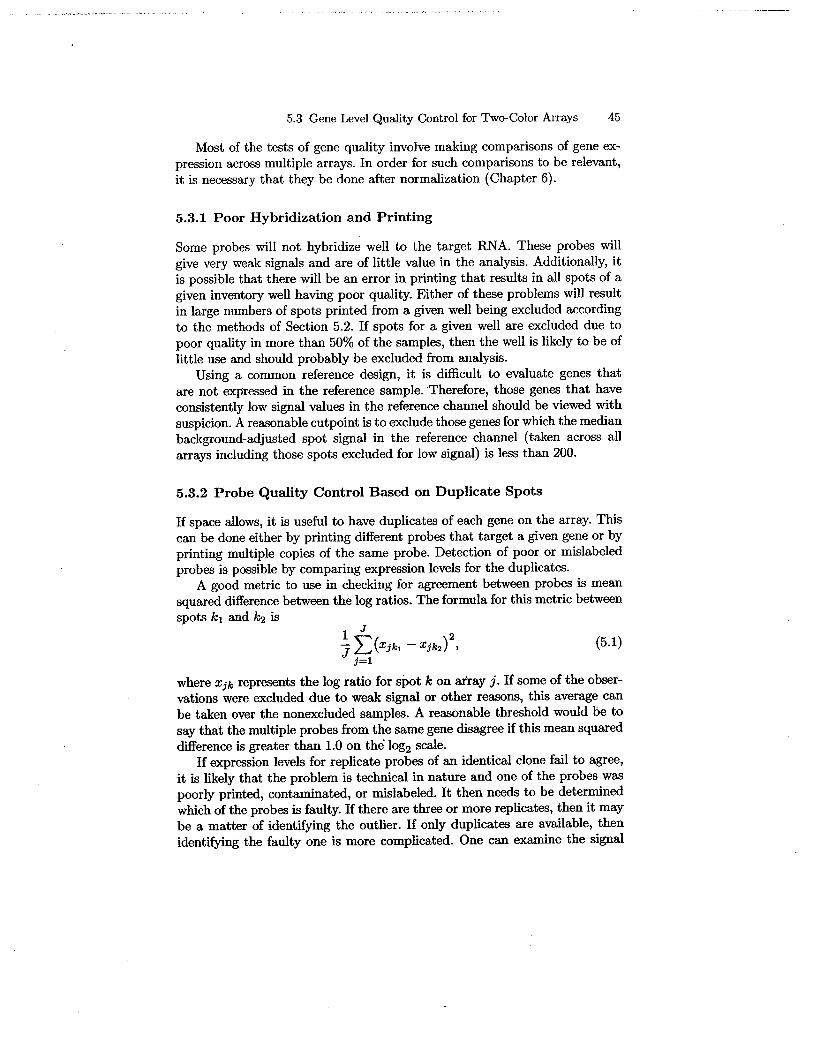
5.3 Gene Level Quality Control for Two-Color Arrays 45

Most of the tests of gene quality involve making comparisons of gene ex-pression across multiple arrays. In order for such comparisons to be relevant,it is necessary that they be done after normalization (Chapter 6).

5.3.1 Poor Hybridization and Printing

Some probes wil not hybridize well to the target RNA. These probes willgive very weak signals and are of little value in the analysis. Additionally, itis possible that there wil be an error in printing that results in all spots of agiven inventory well havig poor quality. Either of these problems wil resultin large numbers of spots printed from a given well being excluded accordingto the methods of Section 5.2. If spots for a given well are excluded due topoor quality in more than 50% of the samples, then the well is likely to be oflittle use and should probably be excluded from analysis.

Using a common reference design, it is diffcult to evaluate genes thatare not expressed in the reference sample. 'Therefore, those genes that haveconsistently low signal vaues in the reference channel should be viewed withsuspicion. A reasonable cutpoint is to exclude those genes for which the medianbackground-adjusted spot signal in the reference channel (taken across allarrays including those spots excluded for low signal) is less than 200.

5.3.2 Probe Quality Control Based on Duplicate Spots

If space allows, it is usefu to have duplicates of each gene on the array. Thiscan be done either by printing different probes that target a given gene or by

printing multiple copies of the same probe. Detection of poor or mislabeledprobes is possible by comparing expression levels for the duplicates.

A good metric to use in checking for agreement between probes is meansquared difference between the log ratios. The formula for trus metric betweenspots ki and k2 is 1 J 2JL(Xjki-Xjk2)' (5.1)j=i

where Xjk represents the log ratio for spot k on may j. If some of the obser-vations were excluded due to weak signal or other reasons, this average canbe taken over the nonexcluded samples. A reasonable threshold would be tosay that the multiple probes from the same gene disagree if this mean squareddifference is greater than 1.0 on the' 10g2 scale.

If expression levels for replicate probes of an identical clone fail to agree,it is likely that the problem is techncal in nature and one of the probes waspoorly printed, contamiated, or mislabeled. It then nee to be determinedwruch of the probes is faulty. If there are three or more replicates, then it maybe a matter of identifng the outlier. If only duplicates are avalable, thenidentify the faulty one is more complicated. One can exame the signal


intensities and background levels of the two spots and look at the correlationbetween each duplicate and genes on the array with similar biology.

When there are probes printed from different clones of the same gene,then differences in expression level may be biological in nature. Because dif-ferent clones may come from different regions of the gene, they may hybridizedifferently to the same transcript. In addition, mutations or deletions of thegene or post-trancriptional modifications may lead to real differences in theabundance of target transcripts for the clones.

Jenssen et aL. (2002) describe an adaptive method for establishing thethreshold for spot exclusion based on a sufcient number of clones printed induplicate on each array. The mean squared difference between duplicates iscomputed for each gene, and averaged over the genes with duplicate spots.Thi variance is computed as a function of filter thresholds. A threshold levelis selected so that 90% of unfiltered duplicate spots on the same array differby less than twofold.

5.3.3 Low Variance Genes

Although not necessarily of poor quality, probes that have low variance of logratio expressions across samples are of questionable utilty. For such genes, theobserved variabilty is more likely to be due to measurement noise than actualbiological variabilty. Although these such genes are very useful in tasks suchas normalization, it may be best to exclude them from analyses that com-pare samples or groups of samples, or that cluster samples; they are likely tobe uninformative and their inclusion can exacerbate the problem of multiplecomparisons (see Chapter 7). Also, computations are faster if there are fewergenes involved, particularly computations involving hierarclucal clustering ofgenes. Potentially, there exists a gene or genes that exlubit a very narrowrange of vaiation but whose tiny fluctuations are exquisitely inormative ofimportant biological distinctions. Unfortunately, the abilty to obtain suff-

ciently precise measurements for such genes might be beyond the techncalcapabilties of curent microarray technologies.

To screen out genes exhibiting little variation across microarray experi-ments, sometimes referred to as nondijJerentially exressed genes, a numberof different approaches are us. Probably the most common approach is to

." set a threshold for fold-change. For example, for each gene take the highestexpression measurement for the gene (across the series of arays) and divideit by the lowest expression measurement for that gene. Any genes for wluchtlus fold-change is less than a threshold such as two or fourold are deletedprior to analysis. A litation of tlus approach is that it does not account

for the number of microarrays in the experiment or the number of genes thatare examned. As either the number of microarrays or the number of genesincreases, the number of truly nondifferentialy expressed genes that exceedany fied threshold will increase.

5.4 Array-Level Quality Control for Two-Color Arrays 47

To account for the number of microarrays, one can take a more statis-tically based approach such as using the ratio of the 95th percentile to the5th percentile rather than a maxImin ratio-based criterion. Taking percentilesremoves the dependence of the expected maxmum and minimum on the num-ber of microarrays, and it is more robust to the infuence of a few extremeobservations.

Alternatively, a variance-based criterion can be used. The variance of thelog ratios for a gene across multiple samples is calculated, and all of thosegenes whose variance falls below a particular threshold are excluded. There areseveral ways to choose a threshold. One could choose an arbitrary number, forexample, exclude all genes whose variance is less than 0.5 on a 10g2 scale. Onecould choose a threshold so that a specified percentage of genes is included,

for example, include only genes with variance in the top 30th percentile; thechoice of percentile wil depend on the composition of the genes included onthe array. A similar approach is to compute the proportion of the arrays forwhich the expression level of the gene is at least twofold diferent from themedian for that gene. Genes for which that proportion is too low, say lessthan 10%, may be excluded.

5.4 Array-Level Quality Control for Two-Color Arrays

An individual array can fail in many ways. Array fabrication defects, problemswith RNA extraction, failed labeling reaction, poor hybridization conditions,and faulty scanning can all lead to an array that is of poor overall quality. Ingeneral, it is better to discard or redo such arrays rather than to risk pollutingthe good data avalable on the other arrays.

One indicator of poor array quality is the number of spots on the arrayexcluded due to poor qualty. A certain number of excluded spots is to beexpected given the multitude of diffculties that can lead to a spot being

poorly measured. Many of the excluded spots will correspond to clones thatfailed to hybridize in any of the arrays. Even afer the poor clones have beenremoved, it is not unusual to fid arrays on which as many as 30% of the spotsare excluded due to weak signal or other reasns. However, if the experimenterfinds that one of the arays has an unusually high number of excluded spots,a number well outside the range of the other arrays, then that sample shouldeither be rearrayed or excluded from analysis.

Another indicator of overall array qualty is the ratio of the average of theforeground intensities of the spots on the aray, and the average of the back-ground intensities of the spots on the array. Higher-quality arrays generallywill have relatively large vaues for this ratio. A value of three or more in bothchanels can generally be considered a good array, and a ratio less than twoin either channel is likely to indicate an array of poor quality.

A thid indicator of poor array quality is very low vaiance of red orgreen intensities across the spots represented on 'the array. Generally, there


should be a substantial range of intensities for each channeL. Assersohn et

al. (2002) recommended that if the standard deviation of the lOglO channel-specific intensities did not exceed 0.25 (corresponding to a standard deviationof 0.83 for 10g2 intensities), then one should suspect the quality of the arrays.

A fourth indicator of array quality is the number of saturated pixels. Asmentioned in Section 4.1, photon intensities may reach a range beyond thelimits of analogue-to-digital converters. In these cass a signal is reported thatis equal to the largest value that can be represented. This necessarily leads toan underestimation of the true output signaL. A few spots with saturated pixelsare to be expected. However, if significant numbers of spots with saturatedpixels are observed (e.g. if more than 2% of the spots on the array have morethan half of their pixels saturated), then it may be best to rescan the arraywith a lower PMT voltage.

One final indicator of array quality is the amount of adjustment requiredfor the array. Data normalzation, discussed in Chapter 6, is used to correctfor biases between different arrays on the same experiment. If it is foundthat the observed signals on a given array nee to be substantially changedto make the array comparable to the other arrays, it is likely that there isa problem on that array that may not be correctable by normalization. Areasonable criterion would be to be suspicious of any array for which a linearnormalization of more than threefold (:11.6 on the log2 scale) is required. Forcases in which the normalization factor varies between genes within an array(location-based or intensity-based normalization) it is reasonable to requirethat no more than 10% of the points require normalization by more thanfoùrfold (:12 on the 10g2 scale).

5.5 Quality Control for GeneChipTM Arrays

The above discussion was directed primarily to two-color cDNA microarrays.Some of the techniques can be applied to Affetrix arrays, but many are

diffcult to implement because the measure of expression of a single geneis based on multiple probe pair measurements. Some useful quality controlmeasures are implemented in softwae such as Afetrix's Micro Array Suite

(MAS), or the dChipl softare created by Li and Wong to aid in qualitycontrol. In this section we describe several of the MAS and dChip qualitycontrol measures and make some additional suggestions.

As with two-color arrays, an initial visual inspection of the array image isan important first step. From the viual inspection of the array image one cancheck the overall quality of the array, check to be sure that the gridding wassuccesfu, and identify any obvious anomalies (bright or dark patches, edge

effects, debris, etc.). Probe pairs in regions that are contaminated by suchanomalies can then be flagged and excluded from the analysis.1 http://biosun1.hard.edu/complab/dchipf.

5.5 Quality Control for GeneChipTM Arrays 49

Each gene in a GeneChipTM array is represented by multiple probe pairs,which are scattered across the array, therefore, gene-level quality control forindividual arrays is more complex than for cDNA arrays. Fortunately, a num-ber of software packages can assist in this quality control. The algorithmMAS uses will down weight individual outlying probe pairs in forming its sig-nal measurement for a given gene. The dChip software (Li and Wong 2001a)attempts to model the relative sensitivity of different probe pairs with regardto their abilty to measure gene expression and then discards as poor quality

those probes that do not fit the modeL.

A number of other quality control indices are available through MAS..MAS report the average background of the array. As with two-color arrays,Affmetrix arrays with high background are more likely to be of poor quality.A reasonable cutoff would be to exclude arrays with a vaue more than 100.A second measure of array quality is the raw noise score, which is referred toas Q by the MAS software. Thi is a measure of the variabilty of the pixelvalues within a probe cell averaged over all of the probe cells on an array. Thisvalue will vary from scanner to scanner, so it is diffcult to provide a unversalcut point. A reasonable approach would be to exclude those arrays that havean unusually high Q-value relative to other arrays that were processed withthe same scanner.

Along with a measure of gene expression, the MAS software produces acall as to whether the gene transcript is present or absent in the sample, andprovides a p-vaue for this cal. This p-value is based on a Wilcoxon signed-ranked test between the perfect match and the mismatch probe intensities.If most of the perfect match probes have larger intensity than the mismatchprobes, then this is an indication that the gene is present. On the other hand,if the distributions of the perfect match and mismatch probes largely overlap,then this would indicate the gene is absent from the sample. Because there maybe correlations between probe intensities, the p-value reported is not strictlyvalid and should not be diectly used as a measure of statistical signficance.Stil, the present/absent call may be a useful tool for screening genes and

detecting problems with the array.Any gene that is absent from the sample should have a true expression of

zero. Any fluctuation in the signal of such genes is therefore due to noise ratherthan any true expression difference. Unle spots on cDNA arrays that havelow expression in both channels, these probe sets are informative because theirlow signals do represent low gene expression. However, comparing expressionlevels across multiple arrays in which the gene is absent is not liely to be

fruitfu. Therefore, if a gene is called absent on alost al of the samples,it may be of little use and should probably not be included in the analysis.Nevertheless, an exception should be made if those few arrays on which thegene is present have a very strong signal. In this case the gene may makea clear distinction between the two sets of arrays (one in which it is clearlypresent and one in which it is absent) and so should be retained in the analysis.


The number of genes that are declared absent on a given array will clearlydepend on the type of tissue being analyzed and the type of array being used.However, if one of the arrays has an unusually large number of absent genesrelative to the other arrays in the experiment, then the array may have failedto hybridize well.

In addition, there are several spiked controls (bioB, bioC, bioD, and cre)that are included in the sample as part of the GeneChipTM protocol. BioB isincluded at a concentration that is close to the level of detection of the array,and so should be indicated as present about 50% of the time. The remainingspiked controls are included at increasingly greater levels of concentration.Therefore, they should all be indicated as present, and also should have in-creasingly large signal values:

Signal(bioB) ~ Signal(bioC) ~ Signal(bioD) .: Signal(cre).

If these spiked controls are declared absent by the MAS software, or havevalues that are not ordered as above, there was either a problem with thehybridization of these controls or a failure to follow the prescribed protocol.In either case, it would probably be best to exclude the array.

As with two-color arrays, the amount of normalzation required is an in-dicator of array quality in GeneChipTM arrays. Unlike two-color arrays, thereare several ways in which to choose a baseline against which to normalizea GeneChipTM array; see Section 6.4. For this reason, we canot suggest anupper limit to the amount of normalization that is acceptable. What is impor-tant is that all arrays have approximately the same amount of normalization.If one array has a normalization factor that is more than three times as largeas other arrays in the experiment, then the array may be poorly measured.

In the case of GeneChipTM arrays, much of the gene quality control hasalready been done by Affetrix. They have done their best to weed outoligonucleotides that have failed to reliably correlate' with gene expression.Stil, if there are genes for which multiple probe sets are available, it is worth-while checking to see whether the expresions for the different versions of thegene agree. As with two-color arrays, thi can be done by checking the meansquared difference of the signal value for the duplicates; refer to Section 5.3.2for details.

5.6 Data Imputation

Mter performng the filtering described previously, there wil generaly be alarge number of missing values in the datast. If the analyses that are bein

performed are done on a gene-by-gene basis, then it is best simply to ignorethe samples on which the gene has miing values and analyze each gene basdsolely on samples for which vaues are present. However, some analyses, wibe performed' using multiple genes. In such analyses, excluding all samples

"'.:'_"'~""._""'_.;'~.""~..~~"C~"""'..~=.:""

5.6 Data Imputation 51

missing anyone gene results in few, if any, samples left to analyze. Someof these analyses can be modified to handle missing data, but others mayrequire that the dataset contain no missing values. For such analyses, one

could restrict the analysis to only those genes that are present on all samples,but doing so may eliminate important genes that have missing values on only

a few of the arrays. Under these circumstances, it may be necessary to imputevalues to replace missing data. Because imputation involves comparing geneexpression across arrays, it should be done afer normalization (Chapter 6).

Thère is a large statistical literature concerned with the problem of missingdata imputation. Little and Rubin (2002) give a good overview of general

methods of dealing with missing values. We present two relatively simplemethods of data imputation that have been applied successfully to microarraydata.

The simplest method of imputing missing values is to replace all missingvalues for a gene with the median value of the observed values for that gene.For two-color arrays, one imputes log ratio vaues. Median vaue imputationhas the advantage of providing a relatively neutral result for the missing data,and so these imputed vaues will not heavily influence conclusions drawn fromthe data. However, inasmuch as there is no biological connection between thesample and the imputed array value, including these imputed vaues in theanalysis will tend to dilute any real effect observed in the other samples. Thismethod may also have the disadvantage of creating a potentially large subsetof samples all of which share identical values for a gene. This could causediffculties for certain analyses that make use of the distribution of a gene'svalues.

A second method of imputation uses the inherent correlation between ex-pressions of different genes on the array to provide an educated guess as tothe correct value for missing genes (Troyanskaya et aL. 2001). This methodis a vaiation of K-nearest neighbor prediction and is implemented as fol-

lows. Assume that we wish to imput,e a value for a gene in sample m andlet Y = rYi,..., YJ J represent the vector consisting of the normalized log

ratios for thi gene across all arrays in which its vaue is present. Let Ym

be the missing value we wish to impute. Calculate the mean squared difer-ence (MSD) distance between Y and every other gene X. In this calculationyou utile every sample that is not missing vaues in either Y or X. Iden-

tify the N genes most simar to the gene whose vaue you need to imputewith respect to this distance. For Ym we impute the weighted average of theexpression for these genes on sample m. The weights are the reciprocals ofthe distances. Troyanskaya et al. (2001) found that a value for N between 10and 20 worked well for their data. Software for thi method is avalable at

http://smi-web.stanord.edu/projects/heli/pubs/impute.Thi method has the advatage that it alows the imputed vaue to be

infuenced by the biology of the sample and so may be less likely to dilutetrue effects than the us of the median for the gene. In addition, because theimputed values wiU differ from sample to sample, this method wi not lead to


many samples sharing the same values for a gene. 'Ioyanskaya et al. (2001)showed that the imputed values generated by this method are more accuratethan using the median when samples are missing at random. Therefore, thismethod will work well for spots that were excluded due to bubbles, scratches,or other array anomalies that are caused more by the location of genes on thechip rather than signal quality. It is not so clear that this method performsas well when samples are missing due to low signal intensity. If a spot on anarray is missing due to low signal, it is likely that many other samples wilalso be miing vaues for this same gene that may make it more diffcult toidentify other genes with similar expression. Fuhermore, those genes thatshare similar expression may als have low signals and be missing for thatsample. As a result, the genes that are averaged to form the imputed valuemay not be very close in expression to the gene for which the value wasimputed and may themselves not be of good quality.

6

Array Normalization

6.1 Introduction

Before comparing the gene expression values between arrays, the arrays mustbe normalized. This step is necessary because there is likely to be an observedintensity imbalance between RNA samples, which wil afect all genes. Thisimbalance has nothig to do with the biology of the samples, but insteadoccurs for a variety of technical reasns, such as differences in the setting of thePMT voltage, imbalance in the total amount of RNA available in each sample,or differences in the uptake of the dyes. The amount of normalization requiredwill vary from array to aray. The objective of normalization is to adjust thegene expression values of all genes on the array so that the genes that are not

really differentially expressed have similar vaues across the arrays. There aretwo decisions that nee to be made: which genes to us as the normalizationgenes and which normalization algorithm to use.

6.2 Choice of Genes for Normalization

Ideally, we wish to normalize using genes that have similar expression acrossour samples. If this is not the case, we ru the risk of confin true biolog-ical diferences in which we are interested with the artifacts we are tryg toelimiate by normalization. Several strateges can be used to obtai a set of

genes on which to base the normalzation.

6.2.1 Biologically Defined Housekeeping Genes

Housekeeping genes are genes that are involved in the essential activities ofcell maintenance and surva, but which are not involved in cell fuction orproliferation. Because all cell nee to expres these genes to surve, it is rea-sonable to expect that such genes wi be similarly expressed in all samples in

54 6 Array Normalization

the experiment. Therefore, such housekeeping genes make perfect candidatesto use in normalization.

Unfortunately, it is often diffcult to identify housekeeping genes. In ad-dition, genes that are housekeeping genes for one type of tissue may not behousekeeping genes for a different type. Therefore, unless carefully controlledexperiments have been performed demonstrating that the expression of thegene is high and approximately constant for the type of tissue being studied,it cannot be known for sure whether the gene can be appropriately considereda housekeeping gene.

The GeneChipTM arrays contain genes that AffetrIx claims to be house-keeping genes. These genes were tested on a large number of different tissuetypes and were found to have quite low variabilty in the tested samples. Theseare certainly good candidates to use as housekeeping genes, but because it isimpossible to test all possible tissue types, there is stil no guarantee that thegenes wil be biologically invariant in every experiment. Therefore, if it is de-cided to use these housekeeping genes to normalize the data, it is worthwhilechecking to be sure that, after normalization, all of these housekeeping geneshave low variabilty across the set of samples used in the experiment.

6.2.2 Spiked Controls

A second method of array normalization is to include in both the reference andthe control samples some RNA that is generally not found in either sample,for example, putting some yeast RNA into human samples. By placing thesame relative amount of RNA into both samples hybridized to a two-colorarray, it is possible to create an artificial housekeeping gene that wil haveequal expression in both channels. If these artifcial genes are spotted on thechip, we will be able to detect bias and be sure of the fact that it was not dueto biological dierences.

The diffculty with thi method is that in order for it to provide the correctnormalization, it is necessar that the proportion of sample RNA to spikedcontrol be the same in both chanels. This implies that the experienter mustbe able to determine the actual amount of RNA included in each channel,and then be able to add the foreign ;R A proportionally. Doing so may betechncally challenging.

The Affetri GeneChipTM protocol includes the spikig of controloligonucleotides into each sample. These controls are included to aid in mea-surng the effectiveness of hybridization and to aid in the griddig of the

slide by the image analysis softe. There is no fied relationship between

the amount of control used and the amount of available RNA in the sample,therefore these controls should not be usd for normalation. FUthermore,the investigator should not be concerned if, even after normalization, the ex-pression of these controls vaies from slide to slide.

6.3 Normalization Methods for Two-Color Arrays 55

6.2.3 Normalize Using All Genes

The simplest approach is to use all of the adequately expressed genes for nor-malization. The underlying assumption for this approach is that the majorityof the genes on the array are housekeeping genes. In fact, for the simplestnormalization methods we present (Section 6.3, and 6.4), all that is requiredfor a set of normalization genes is that the proportion of genes that are overexpressed in a given sample be approximately equal to the proportion of genesthat are under expressed. These assumptions wil hold for most randomly se-lected sets of genes. Therefore, this method works well in cases where thereare a.large number of genes included on the array and when the majority ofthe genes were not specifically selected to be differentially expressed betweenthe experimental and reference samples. However, if the genes on the array

were carefully selected to be genes of specific biological interest that are highly

variable across the samples, then it will be necessary to include a separate setof either housekeeping genes or spiked controls to us in normalization.

6.2.4 Identification of Housekeeping Genes Based on ObservedData

There are several technques for using the observed data to identify housekeep-ing genes. For two-color arrays, Tseng et aL. (2001) recommend designating ashousekeeping genes those genes that have similar rans in the red and green

channels. We find that such techniques often choose those genes that are in thecenter of the distribution of all log ratios on the array. Therefore, the resultof normalizing with respect to this subset is vitually identical to the resultobtained by normalizing with respect to the complete list of genes. Wang etaL. (2002) present an iterative method for selecting normalization factors andsimultaneously identifyng genes with low variation across the arrays afternormalization.

6.3 Normalization Methods for Two-Color Arrays

Normalization of two-color arrays involves determiation of the amount bywhich the genes on the red chanel are over- or underexpressed relative to thegreen chaneL. This bias wi difer for diferent arrays and, dependig on theform of the bias, may vary by gene. Once the siz of the bias is estimated,we obtain oUl final signal value by subtracting thi normalization factor fromthe,observed log ratio. Thus the normalze signal value for clone k on arrayj will be

(R-k)Xjk = log -i - Cjk,

Gjk

where Rjk and Gjk denote the background-adjusted red and green signal asin Equation (4.1) and Cjk is the normalation factor.


There are several ways of calculating Cjk. These methods differ in theirmodeling of the systematic bias to be corrected by normalization. They canbe divided into three categories: linear or global normalization in which thenormalization factor is the same for all genes on the array, intensity-based

normalization in which the normalization factor used depends on the signalintensity for that spot, and location-based normalization in which the normal-ization factor depends on the location of the spot on the array. Determiningwhich type of normalization method to use requires examining the observedunnormalized log ratios and deciding what kinds of systematic effects arepresent. The amount of normalization requied wil vary by array. Thereforeeach array should be normalized separately. However, the type of normaliza-tion used (linear, intensity, location) should be the same for all arrays in theexperiment.

\6.3.1 Linear or Global Normalization

The simplest method of normalization uses a single normalization factor ap-plied to all genes on the array, but thi vaue varies from array to array. Itis called linear normalzation because it assumes that the red and green in-tensities have an approximately linear relationship through the origin for thenormalization genes on a given array. The slope of thi linear relationship willdetermine the amount of normalization required, and will become an additiveeffect on the log scale.

For this normalization method, all genes on a given array will have thesame normalization factor. The formula for linear normalization is

Cjk = Cj = m~dian (iog (GRjk)),iES jk (6.1)

where S is the set of normalzation genes. We use the median rather than themean because it is less likely to be infuenced by outlyig values. Als, if weare normalizing with respect to all genes, then accordig to our assumptionsregarding the distribution of up-and down-reguated genes (see Section 6.2.3)the center of the distribution of log ratios should consist of those genes thatare not differentially express between the red and green channels. By usingthe medan, we focus attention on these center genes. ,

This method works well for most applications. It wil be usable even whenthere are a relatively smal number of normaliation genes (e.g. 50 to 100genes), as is often the case when housekeeping genes or spiked controls areused. Thi method also has the advatage that it is les Ìiely than othermethods to over fit the normalation to the data. Other methods in whichthe normalization vaies from gene to gene are more sensitive to chanes in theobserved exression of individual genes, and so may produce bias results.For thi reasn, we recommend linear normalization uness there is compellngevidence that a substantial number of arrays in the experiment require a morecomplicated normalization method.


6.3.2 Intensity-Based Normalization

In some arrays, it appears that the overall magnitude of the spot intensitymay have an impact on the relative intensity between the channels. In orderto determine if this is the case, it is recommended that the experimenterlook at so-called M-A plots (Yang et aL 2002a) in which for each array j thequantity

Mjk = log (~~:)

is plotted against the RNA abundance

1Ajk = '2 (log(Rjk) + 10g(Gjk))

over all normalization genes. In the above equations Mjk represents the logratio of background-adjusted intensities for gene k on array j. Ajk representsthe average of the red and green channels with regard to background-adjustedintensity for gene k on array j.

If no normalization is required, the spots will appear symmetrically scat-tered around the horizontal line M = O. If only a linear normalization isrequired, then the spots wil stil be scattered around a horizontal line, but

the line will be shifted up or down away from 0 by an amount equal to therequired normalization. Figure 6.1(a) shows such a plot. If the spots follow aline with nonhonzontal slope, or a nonlinear curve, then it may be necessaryto perform a nonlinear intensity normalization. Figure (6-1 (b)) shows such aM-A plot. In this case, the spots with lugh intensity (high A values) have arelatively smaller red signal than green signal (negative M vaues).

The techncal caus of this nonlinearity in normalization is not immedi-ately obvious. It may have to do with a component of background lumines-cence that acts in a nonadditive way with the foreground, or it may have to dowith some aspect of signal saturation in the detector. Whatever the cause, theform of the normalization curve can va markedy between arrays. Thereforeit is necessary to fit a separate normalization cure to each array.

If it has been determined that intensity-based normalization is necessar,the next step is to fit a curve to t~e M-A plot for the normalization genes.Locally weighte regresion curves (also known as loes curves) are most fre-quently usd, but other smoothig fuctions such as splines should produce

similar results. The lines in Figues 6.1(a) and (b) show the loess normaliza-tion curve fitted to the data.

Once the cure is fitted, we defie

Cjk = h(Ajk),

where h is the smootlung fuction fitted to array j, and Ajk is the abundancevalue for clone k on array j.

In order to perform intensity-bas normalization, it is necessary thatthere be normalization genes across al intensity vaues. Therefore if there are


Figure 6.1a M-A plot with Loess fitLinear Normalization acceptable

7

5.~ -':-.' :- y

3

. ,::

.'! ,~~... . , ..

-1 "-. .

-3

-5o 2 4 6 8

A

(a)

10 12 14 16

Fi~uré;6.1b M.,AplötWith loeSS fit,Iïiíeïis¡' ,basédN'oalfiaiòn"rEiiiired

10

5

:2 Ö

,5

-10

o :2, 4 'l¡' 8 10 12 14 16

A

(b)

Fig. 6.1. (a) Loess fit to M-A plot of aray data. Horiontal loes line indicates that

consant normtion should be sufcient. (b) Lo fit to M-A plot of aray data.Clea nonlnearity of loes fit indicates that intensty-bas normalation should beus.


only a small number of identified housekeeping or spiked control genes, orif the expressions of these genes do not span the range of expression levels,this normalization method cannot be used. Furthermore, even if all genes arebeing used to normalize the data, there is the implicit asumption that at eachintensity level there are equal numbers of up- and down-reguated genes. If allthe high- (or low-) intensity genes share similar biology, it is possible that thisassumption could be violated and it would be best to avoid thi normalizationmethod.

Another danger of using intensity-based normalization is that at intensitiesfor which there are few spots the normalization could be based on a rathersmall number of points, and as a result could overfit to those particular values.Thus, by normalizing the data, the experimenter could subtract away exactlythe effect he or she was tryng to measure if the normalization was performedusing all genes.

6.3.3 Location-Based Normalization , /Another artifact that is sometimes observed is that the background-subtractedlog ratios on the array va in a predictable manner based on their position onthe array. Figure 6.2(a) shows the dependence between log ratios and positionon a sample array. The spots along the top and right side of the array appearto be very red, and the lower left corner appears much less red.

One factor that may contribute to location-specific differences in the ob-served log ratios are differences in the print tips used to create the slide.Because there may be subtle diferences in the degree of wear on a print tip,it has been suggested that normalzation should be performed separately foreach print tip (Yang et al. 2002a).

Figure 6.2(b) shows the median log ratio for each of the 24 grids in thearray presented in Figure 6-2a. The lower left grid has a lower median logratio, as do those around it, and the grds on the top and right side havelarger vaues. Each print tip generates a grid that is located at a separateplace on the array. By normalizing with respect to the print tip, we effectivelynormalize with respect to many of the location differences as well.

To normalize within the grid we apply Equation (6.1) but take the medianonly over the normalzation genes withi the grid. Figue 6.2(c) shows the

results afer location normalzation. There is now no clear location dependencefor the log ratios.

In order to perform location-based normalization, it is necessar that therebe significant numbers of normalization genes withi each grid. Therefore thistechnque will not be applicable for normalizing with respect to a small numberof spiked controls or housekeeping genes. In addition, inasmuch as there arefewer genes in each grd than there are on the entire array, there is the same

danger of overftting as there was in the intensity-based normalization.

It is possible that normalizing with respect to the print tip wil not com-pletely account for all location effects. Although more complicated methods of


Figure 6,2alogratio by poitionbefore norma lization

350

30

2500

20

150

1000

50

100 60 1100 1600X

(a)

"igure6.2~log rao, by poitionaftr normalization

350

30

itôo

1Ö,.' ,r

150

.500.

Figure 6.2bnormalization witin each grid

30

~~

100

oo 50 100 150

(b)

netx

(c)

Fig. 6.2. (a) Plot of log ratio for eah location on the aray before normaliation.High emichment for red along the top and right sides indicates possible need forlocation-based normalation. (b) Location normalzation factors of eah grid foraray depicted in Figue 6.2(a). (c) Plot of log ratio for eah location on the arayafer location-basd normalzation. Red and green signals are now dispersed evenly

across slide.

6.4 Normalization of GeneChipTM Arrays 61

location-based normalization exist, many involve the estimation of numerousparameters, and may introduce artifacts by overfitting the data.

6.3.4 Combination Location and Intensity Normalization

If it appears that both location and intensity-based normalization are re-

quired, there are two ways to procee. One possibilty is to perform linearnormalization separately for each grid and then apply intensity-based nor-malization to the resulting normalized log ratios on the entire array. Alterna-tively, the intensity-based normalization can be performed separately withineach grid. Yang et aL. (2002a) reported that the shape of the loess curves fitto the M-A plots could vary from grid to grid, suggesting that the secondalternative might be best. However, the number of available spots within eachgrid may be relatively low, makng the fitted curve dependent on the valuesof a few points. This is particularly a problem at intensities where data aresparse. Thus there is a danger that true biological variabilty of an individualspot may be absorbed by the normalization factor and eliminated. Therefore,unless it is very clear that the patterns of the M- A curves va significantlybetween grids on the array, we recommend using a single M-A plot fitted toall spots on the array.

6.4 Normalization of GeneChipTM Arrays

As with two-color microarrays, the overall magntude of the signal for all geneson a given Affetrix array can vary for techncal reasons unrelated to bi-ology. Therefore normalization is necessary. Unlike two-color arrays, there isonly a single channel in oligonucleotide arrays. This mean that some tyes ofnormalization on Affetrix data must be done between arrays rather than

within a single array. Stil, many of the same issues that confronted us intwo-color array data carryover to Affetrix data. Both linear normalization

methods and intensity-based algorithm have been applied to GeneChipTM ar-rays. However, location-specific normalization is generally not used. Althoughlocation-based intensity imbalances may exit, such imbalances are generalyless severe for Affetrix arrays because the sample is circulated over the sur-

face of probes. Also, because the probe pairs for a gene in Affetrix arraysare scattered across the array, location-bas imbalances wil have a smalereffect on the mean diferences of individual genes than they did in the caseof two-color arrays. As with two-color arrays, the normalzation vaues shouldbe calculated separately for each array, but the normalation method usedto calculate these values should be the same for al arrays.

6.4.1 Linea or Global Normalzation

As with two-color arrays, the simplest method of normalzation is to use asingle normalization factor for all genes on the array. Thi method is used by


Affymetrix's MAS software. This software gives the user the abilty either tochoose a particular target signal value or to choose a particular baseline arrayagainst which to normalize. Based on this choice, the normalization signal log

values are calculated as follows.

(normalized signal log value)jk = SLVjk -log2(s!i), (6.2)

where SL V denotes the signal log vaue for gene k on array j given by expres-

sion (4.3) and sfj is the scaling factor for array j. The signal vaue reportedby the MAS software is 2 raised to the power of normalized signal log value.

Affmetrix software computes the scaling factor as

sfj = log2(Sc) -log2 (Trim,lean(2SLV;k)) , (6.3)

where Se is the target constant used for normalzing all arrays. The "Trim-Mean" notation denotes the mean of the signal values on array j for thehousekeeping genes, excluding outliers in the upper and lower 2% of the dis-tribution. Affetrix computes the trimmed mean on the absolute intensity

scale. Because SL V is a log2 tranformed value, the value is raised to the

power 2 before taking the trimmed mean. If no housekeeping genes are iden-tified, then the trimmed mean uses the signals for all of the genes on thearray. If arrays are normalized to a fied constant, then Se is that constant.If a baseline array is chosen for normalization, then Se is taken as the 2%trimmed mean of the signals for the housekeeping genes on the baseline array.

As we can see from Equations (6.2) and (6.3), changing the target constantor baseline array only results in a different constant being added to all normal-ized signal log values. Thus it wil have no effect on any comparative analysesbetween arrays provided Se is the same for all arrays being compared. Forthis reason, we recommend that if the MAS normaliation algorithm is used,the experimenter normalize to the default value of 500 as this will faciltatecomparisons between experiments by different investigators.

When considering other normalization methods it should be noted thatthe MAS software performs its own normalization automatically. Therefore,the signals that are obtainable from the MAS softare have aleady beennormalized with their algorithm. Because the MAS normaliation is linear,applying a new normalization to signal that were aleady normalized by

MAS will produce the same results as applyig the new normalzation to theraw signals. Thus, for the purposes of considering alternative normalizationmethods, the MAS output vaues can be treated as the taw signal.

6.4.2 Intensity-Based Normalation

Nonlnear intensity-based normalation may alo be required in GeneChipTMarrays. To determne whether it is necessar, graphs simlar to the M - A plotscan be generated. However, rather than comparing dierent chanels from the

6.4 Normalization of GeneChipTM Arrays 63

same array, pairs of arrays are compared. Let Xk denote the normalized signallog value for gene k on one array and Yk the normalized signal log value forthe corresponding gene on a second array; we plot

Mk = Xk - Yk against Ak = !(Xk + Yk)'2

Because most genes are not expected to vary significantly from array to array,the spots on the plot should be scattered around a horizontal line at 0 if nonormalization were needed. If only linear normalization were required, thespots would lie on a horizontal line at a value other than O. If the spotsare scattered around a nonhorizontal line or a nonlinear curve then this wilindicate the need for an intensity-based normalization. Unfortunately, becausethe form of the graph depends on which arrays are paired, a choice must bemade as to which array to normalize against. Li and Wong's dCHIP softwarechooses a single array of medium intensity and then normalizes the probe-levelintensities of all other arrays to resemble this one.

Other methods of normalization of Affmetrix data at the probe intensitylevel are described and compared by Bolstad et al. (2002). They found thata method known as quantile normalization worked best. This method relieson the assumption that even though there may be dífferences between arrays

in the expression of individual probes, the distribution of the expression val-

ues should not change dramatically between arrays. Futhemore, they assumethat within a single array there is a monotone relationship between the geneexpression level and probe value. Therefore they adjust each array in a mono-tone manner so that all arrays have the identical distribution. The method isas follows. Compute the kth smallest signal value on each array and averagethem over the arrays. Let Xj(k) denote the kth smallest signal on the jth array

and let X(k) denote the average over the arrays oftheir kth smallest signals.Replace Xj(k) with X(k) on al of the arrays. Do this for each k = 1,2,... ,up to the number of probe sets on the array. Thus, afer normalization, allarrays will share the same set of probe signal vaues, but which probe is associated with which vaue will vary from array to ar,ray depending on the ranordering of the gene expressions. That is, the lOOt~ smallest value on array

1 wil be the same as the lOQth smalest vaue on array 2 but they may rep-resent two different probes. This method of normalization is implemented inthe Bioconductor softare avaable at http://ww . bioconductor. org/.

Even if software that processes probe-level data is not used, an intensity-based normalization can be penormed at the sigal leveL. First, a baselinearray is chosen to use as a reference; we recommend using an array whose sfvaue is closest to the median of the sf vaues of the arays being analyzed.The Affetrix MAS5 softare includes the sf vaue for each aray as partof the output. The M-A plots can then be generated as was done in Section6.3.2, using the signal for the array being normalized as if it were the testchanel and the signal from the baseline array as if it were the reference. If itappears that intensity-dependent normalization is neeed, then either quantile

7

Class Comparison

7.1 Introduction

One of the most important goals in microarray studies is to identify genes thatare diferentially expressed between prespecined classes. Identifyng differen-tially expressed genes with known functions can lead to a better understandingof the biological differences between the classes. Identifying differentially ex-pressed genes with unknown functions can lead to a better understanding ofthe fuctions of those genes. The goal of this chapter is different from thatof Chapter 9; the goal there is to create classes of specimens for which geneexpression is different. Class comparion methods are superved in the sensethat they utilze the information of which specimens belong to which classes.

This is in contrast to methods such as cluster analysis discussed in Chap-

ter 9 which utilze only the expression profiles and are unsupervised by anyinformation about class membership.

We begin in Section 7.2 by examining whether a particular gene is differ-entially expressed between classes. This provides the statistical backgroundfor the more realistic problems involving thousands of genes addressed in theremainder of the chapter. Section 7.3 describes how to identify whiCh genes

are differentially expressed while controlling for the large number of genes be-ing examed. Section 7.4 describes some methods of analysis of experimentswhen there are very few specimens in each clas avalable for microarray anal-ysis. Section 7.5 presents global tests of whether there are class dierencesin gene expression without trying to identif which genes are dierentialy

expressed. Section 7.6 addresses the special !lituation in which there is onlyone specimen in each clas. A natural generalzation of clas comparion is to

ask whether gene expression is associated with a continuous characteritic or

a surva time for the individual from whom the specimen was obtained; this

is discused in Sections 7.7 and 7.8, respectively. Section 7.9 ends the chapterwith a dicusion of statistical models for analysis of nonreference design fortwo-color aray experients.

66 7 Class Comparison

7.2 Examining Whether a Single Gene is DifferentiallyExpressed Between Classes

We begin by considering the case of two classes, in which case we wish todiscover whether a gene has higher expression in one clas as compared tothe other. As discussed in chapter 4, analyseS of expression data typically use

logarithmically transformed levels; we use logarithms base 2 for most of ouranalyses. Suppose one has available Ji specimens from class 1 and J2 speci-mens from class 2. Consider a particular gene, with (transformed) expressionsip class 1 given by Xu, X12, . . . , X1J¡ and in class 2 given by X21, X22, . . . , X2J2'One can summarize the average expressions in classes 1 and 2 by the _ meansof the class 1 and class 2 values, Xl and X2. If Xl is larger (smaller) than X2,

this would suggest that gene is expressed more (less) in clas 1 than class 2.There are several things to note about this type of comparison. First, thiscomparison makes sense even if each expression value is relative to a refer-ence standard (as would generally be the case for cDNA arrays), providedthat the same reference standard is used for the specimens in both classes.Second, assuming that the processing of the microarrays is done in the samemanner for both classes of specimens, one does not need to be too concernedabout sources of systematic bias that are present in the microarrays of bothclasses; these biases wil tend to cancel out when comparing the expressionsbetween classes. For example, with cDNA arrays if the reference specimen islabeled consistently with say, Cy3, then there may be gene-specific dye bias

not removed by normalization, but it wil not be of concern in comparing theclasses. It would only be of concern if we wished to compare either class tothe internal reference. Third, only one microarray per specimen is required.If there are replicate arrays on a specimen, we recommend averaging the logexpression vaues to form a single Xij to be used for that specimen, or choosingthe array with the best quality; see Chapter 5. Issues concernng whether todesign a study with replicate arrays are discussed in Sections 3.4 and 3.7.

Because it is unikely that the mean expression levels Xl and X2 will be

exactly equal, how does one know that any difference observed between Xland X2 is not due to chance? Clearly, a larger rather than smaler diferencebetween Xl and X2 suggests that the difference is not due to chance. But howlarge a difference is requied? One possibilty would be to choose a certai folddifference, for example a twofold diference that corresponds to IXi - x21 ;: 1when base 2 logarthmc tranformations are used. Thi was the approach

used by Lee et al. (1999) when comparing gene expresion in 5-month versus30-month-old mice. A problem with thi approach is that it can lea to a

high probabilty of declarig that a gene is differentially expressed when it

truly is not (Miler et aL. 2001). The approaches described in this section use

elementary statistical methods to guard against such chance findigs; readerswith a statistical background may wih to skip all but the examples in theremainder of this section.

7.2.1 t-Test

7.2 Examining Whether a Single Gene is Differentially Expressed 67

In order to guard against chance findings, one must characterize what onemeans by chance. One notion is as follows. There is a very large population ofclass 1 and class 2 specimens, and the distributions of the expressions of theclass 1 and class 2 specimens are the same in the population. This is referredto as the null hypothesis. The Ji clas 1 specimens and J2 clas 2 specimensunder investigation are assumed to be (completely) random samples from theclass 1 and class 2 specimens, respectively. St~tistical theory allows one toestimate the probabilty that one would see a diference as large as observed.There are different methods to do this. The most commonly used involves atwo-sample t-statistic,

where

and for i = 1, 2,

Xl - X2t= ,V s2 (i. + i.)p Ji J2

(7.1)

S2 _ (Ji - l)s¡ + (J2 - l)s~P - Ji + J2 - 2

1 J,s~ = J- -1 L)Xij -Xiti j=1

The variance estimator s~ estimates the (pooled) within-class variabilty ofthe gene expressions; its square root is known as the within-class standarddeviation. An alternative t-statistic uses V sV Ji + s~/ h in the denomiatorof (7.1). This alternative t-statistic is referred to as the t-statistic using theseparate-variance formula, whereas (7.1) is referred to as the t-statistic usingthe pooled-variance formula.

One interpretation of the t-statistic is that it is the ratio of between-clas towithin-class vaiabilty of the gene expression. Another interpretation is thatthe denominator of the statistic is an estimator of the vaiabilty of Xi - X2one would see if one repeatedly sampled Ji class 1 and J2 class 2 specimensfrom the very large population. With either interpretation, large positive ornegative values of the t-statistic suggest that Xi and X2 are difering morethan by just chance. The t-statisic is converted to a probabilty, known as ap-value, which represents the probabilty that one would observe under the null

hypothesis a t-statistic as large or larger (in absolute vaue) than the t-statisticcalculated from the observed data. For example, one would observe p-vauesless than 0.01 under the null hypothesis only 1% of the time. The p-valueis also sometimes referred to as the statistical significance of the data (withrespect to the null hypothesis) obtaied from a t-tet of the nul hypothesis.All of our hypotheses tests and p-vaues wil be two-sided, representing the

fact that we are interested in either class having more expression than theother.

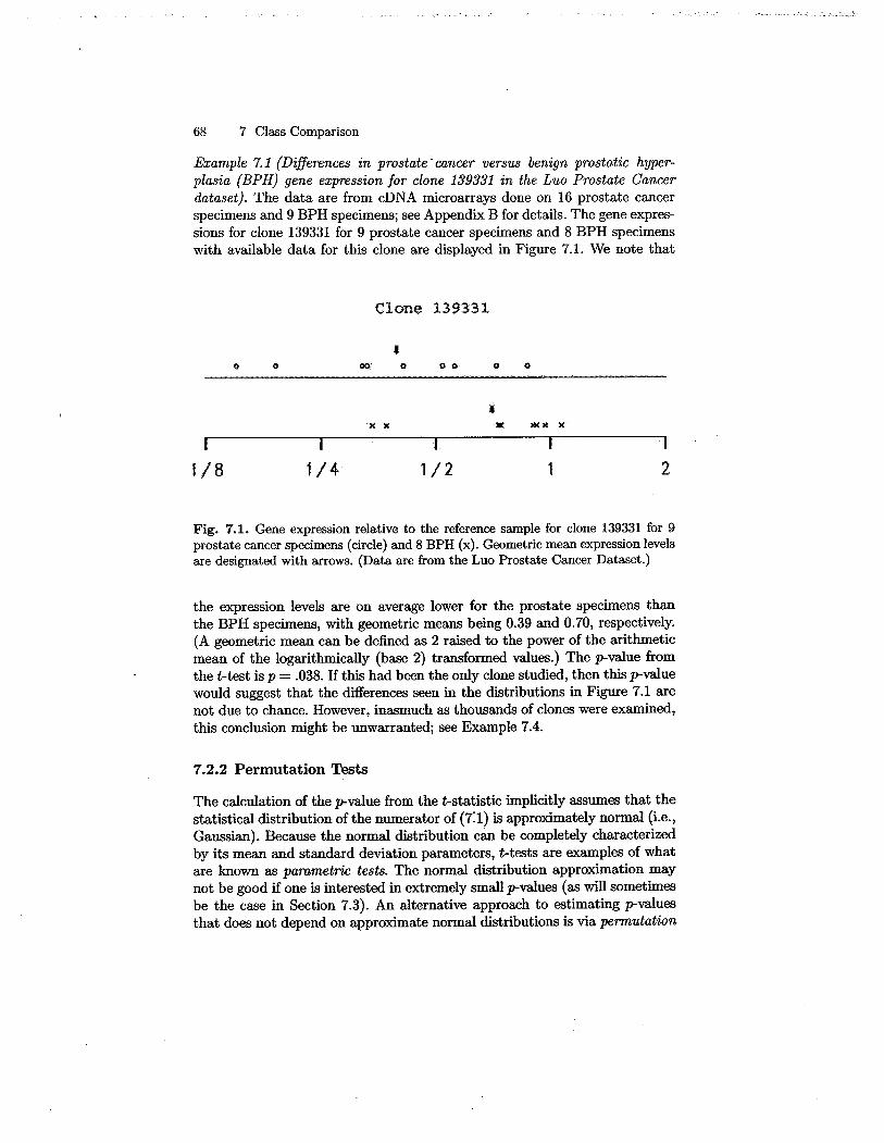
68 7 Class Comparison

Example 7.1 (Differences in prostate - cancer versus benign prostatic hyper-plasia (BPH) gene expression for clone 139331 in the Luo Prostate Cancerdataset). The data are from cDNA microarrays done on 16 prostate cancerspecimens and 9 BPH specimens; see Appendix B for details. The gene expres-sions for clone 139331 for 9 prostate cancer specimens and 8 BPH specimenswith available data for this clone are displayed in Figure 7.1. We note that

Clone 139331

l0 0 00' 0 00 0 0

.x x . *ic x

I I I I I

1/8 1/4 1/2 1 2

Fig. 7.1. Gene expression relative to the reference sample for clone 139331 for 9

prostate cancer specimens (circle) and 8 BPH (x). Geometric mean expression levelsare designated with arrows. (Data are from the Luo Prostate Cancer Datast.)

the expression levels are on average lower for the prostate specimens thanthe BPH specimens, with geometric means being 0.39 and 0.70, respectively.(A geometric mean can be defined as 2 raied to the power of the arithmeticmean of the logarithmcally (bas 2) tranformed vaues.) The p-vaue fromthe t-test is p = .038. If thi had been the only clone studied, then thi p-vauewould suggest that the diferences seen in the distributions in Figure 7.1 arenot due to chance. However, inasmuch as thousands of clones were examned,this conclusion might be unwarranted; see Example 7.4.

7.2.2 Permutation Tests

The calculation of the p-vaue from the t-statistic implicitly assumes that thestatistical ditribution of the numerator of (7:1) is approximately normal (Le.,Gaussian). Because the normal distribution can be completely characterizedby its mean and standard deviation parameters, t-tests are examples of whatare known as parametri tests. The normal distribution approximation maynot be good if one is interested in extremely small p-vaues (as will sometimesbe the case in Section 7.3). An alternative approach to estimating p-vauesthat does not depend on approximate normal distributions is via permutation

7.2 Examining Whether a Single Gene is Differentially Expressed 69

tests. One example of a permutation test, the permutation t-test, is given asfollows. First, the t-statistic is calculated using (7.1). Then the class labels ofthe Ji + h specimens are randomly permuted, so that a random Ji of the

specimens are temporarily labeled as class 1, and the remaining J2 specimensare labeled as class 2. Using these temporary labels, the t-statistic (7.1) iscalculated, say, t*. The labels are permuted many times with a calculation oft* each time. The (two-sided) p-value from the permutation t-test is estimatedby

I 1 + # of random permutations where Wi ~ It Ip-va ue = . (7.2)

1 + # of random permutations

With small sample sizes or in some special cases, one can actually enumerateall

(Ji + h) = (Ji + J2)!Ji - (Ji!J2!)

permutations and use

al _ # of permutations where Wi ~ It I p-v ue - (Ji ~ J2 ) (7.3)

rather than the estimator (7.2). (The symbol J! mean J x (J -1) x (J - 2) x

. .. x 2 x 1.) A schematic example of the calculation using hypothetical datais given in Figure 7.2: With 5 observations in one clas and 4 in the other,there are a total of (;) = 126 possible permutations for the data. For the datashown, the absolute vaue of the t-statistic is 3.64 which is less than or equal to3 of the permuted dataset absolute t-statistics; the t-statistics correspondingto these 3 datasets are shown in bold tye. (Note that the original datasetis considered to be one of the permuted datasets for this calculation.) Thepermutation p-vaue is therefore 3/126 = .024.

Example 7.2 (Permutation t-test for differences in gene exression for clone139331 in the Luo prostate dataset.). This is a continuation of Example 7.1.The gene expressions for clone 139331 for 9 prostate cancer speimens and 8BPH specimens with av.lable data for this clone are diplayed in Figue 7.i.Because there were missing data in thi example (7 prostate cancer specimens

and 1 BPH specimen), there are two different ways to permute the clas labels.One possibilty is to ignore the missing data and randomly assign 16 of theoriginal specimens to be class 1 and the remainder to be class 2. Note that,if done in thi way, the numbers of class 1 specimens with avalable data canchange from permutation to permutation. The other possibilty is to restrictthe permutations to the non-missing specimens and to randomly assign 9 ofthe 17 specimens with non-mising data to be class 1 and the remainder ofthe 17 to be class 2. In this case, each permuted dataset wi have exactly 9class 1 specimens. We recommend using the first method, that is, permutingthe class labels for al the specimens regardless of whether expression data

Documents

Design and Analysis of DNA Microarray Investigations - Biometric