Embed Size (px)
Citation preview
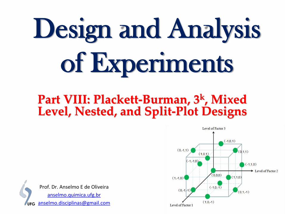
Design and Analysis
of Experiments
Part VIII: Plackett-Burman, 3k, Mixed Level, Nested, and Split-Plot Designs
Prof. Dr. Anselmo E de Oliveira
anselmo.quimica.ufg.br

Plackett-Burman Designs • Two-level fractional factorial designs developed for studying
𝑘 = 𝑁 − 1 variables in 𝑁 runs, where 𝑁 is a multiple of 4
• Nongeometric designs (cannot be represented as cubes)
• Nonregular designs – Regular design is one in which all effects can be estimated
independently of the other effects (e.g. 2k design) and in the case of a fractional factorial, the effects that cannot be estimated are completely aliased with the other effects (e.g. 2k-p design)
• Screening – Main effects are, in general, heavily confounded with two-factor
interactions
– Plackett-Burman designs are very efficient screening designs when only main effects are of interest.
• Web of Science: – 2017/04: 47
– 2016: 202
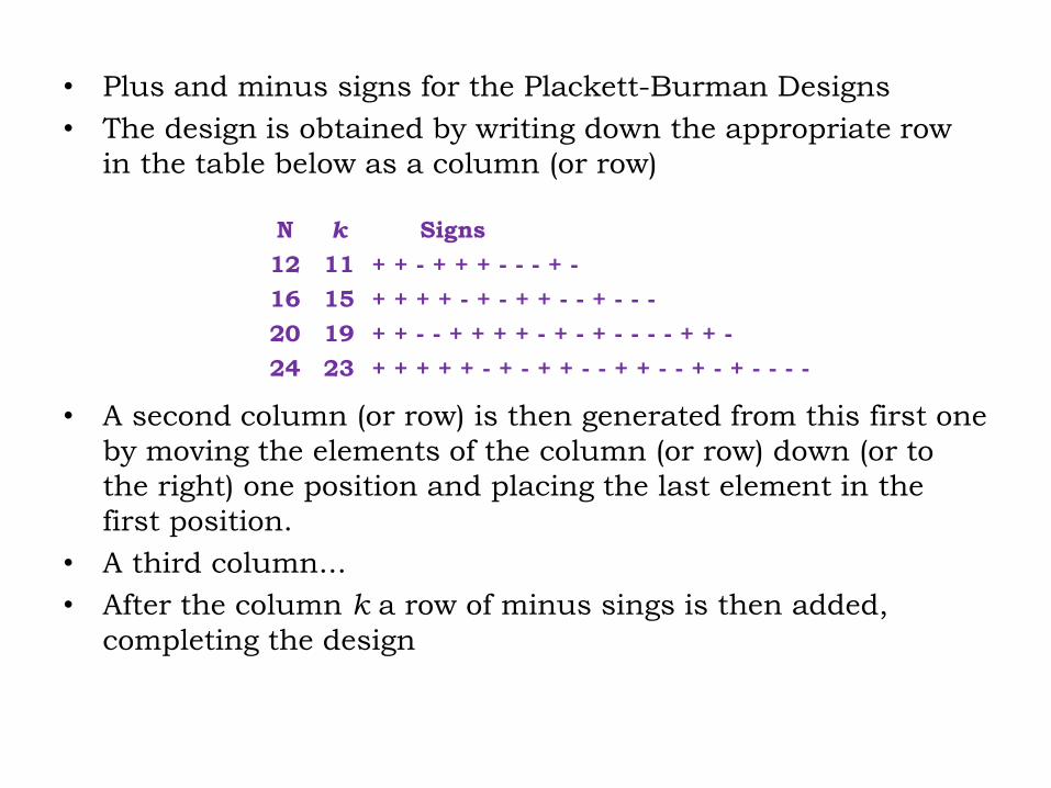
• Plus and minus signs for the Plackett-Burman Designs
• The design is obtained by writing down the appropriate row
in the table below as a column (or row)
• A second column (or row) is then generated from this first one
by moving the elements of the column (or row) down (or to
the right) one position and placing the last element in the
first position.
• A third column...
• After the column k a row of minus sings is then added,
completing the design
N k Signs
12 11 + + - + + + - - - + -
16 15 + + + + - + - + + - - + - - -
20 19 + + - - + + + + - + - + - - - - + + -
24 23 + + + + + - + - + + - - + + - - + - + - - - -
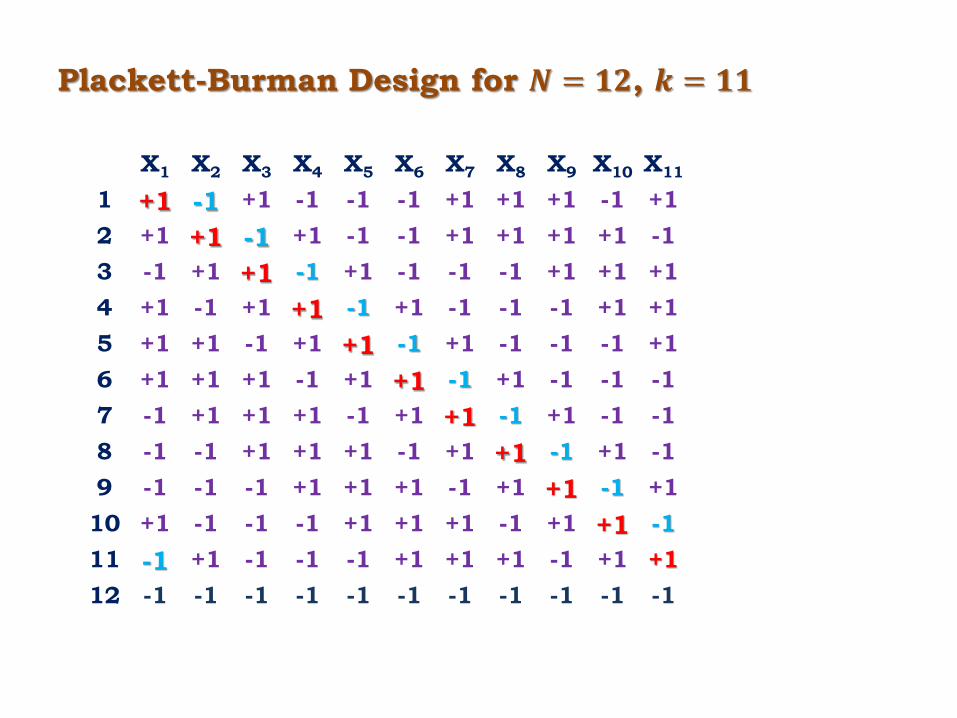
Plackett-Burman Design for 𝑵 = 𝟏𝟐, 𝒌 = 𝟏𝟏
X1 X2 X3 X4 X5 X6 X7 X8 X9 X10 X11
1 +1 -1 +1 -1 -1 -1 +1 +1 +1 -1 +1
2 +1 +1 -1 +1 -1 -1 +1 +1 +1 +1 -1
3 -1 +1 +1 -1 +1 -1 -1 -1 +1 +1 +1
4 +1 -1 +1 +1 -1 +1 -1 -1 -1 +1 +1
5 +1 +1 -1 +1 +1 -1 +1 -1 -1 -1 +1
6 +1 +1 +1 -1 +1 +1 -1 +1 -1 -1 -1
7 -1 +1 +1 +1 -1 +1 +1 -1 +1 -1 -1
8 -1 -1 +1 +1 +1 -1 +1 +1 -1 +1 -1
9 -1 -1 -1 +1 +1 +1 -1 +1 +1 -1 +1
10 +1 -1 -1 -1 +1 +1 +1 -1 +1 +1 -1
11 -1 +1 -1 -1 -1 +1 +1 +1 -1 +1 +1
12 -1 -1 -1 -1 -1 -1 -1 -1 -1 -1 -1

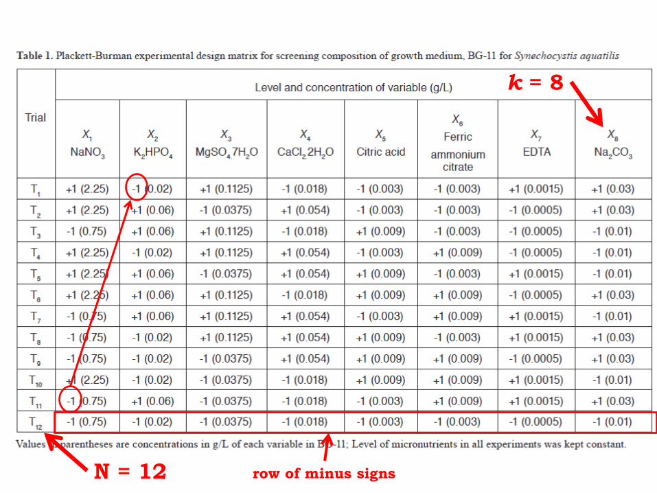
N = 12
k = 8
row of minus signs
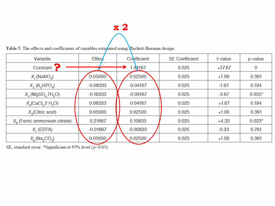
x 2
?
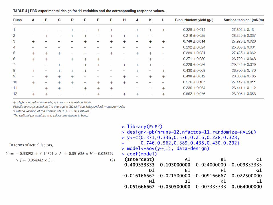
> library(FrF2) > design<-pb(nruns=12,nfactos=11,randomize=FALSE) > y<-c(0.371,0.336,0.576,0.216,0.228,0.328, + 0.746,0.562,0.389,0.438,0.430,0.292) > model<-aov(y~(.), data=design) > coef(model) (Intercept) A1 B1 C1 0.409333333 0.103000000 -0.024000000 -0.009833333 D1 E1 F1 G1 -0.016166667 -0.021500000 -0.009166667 0.022500000 H1 J1 K1 L1 0.051666667 -0.050500000 0.007333333 0.064000000
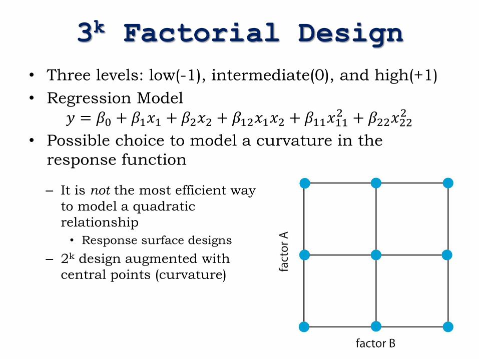
3k Factorial Design
• Three levels: low(-1), intermediate(0), and high(+1)
• Regression Model
𝑦 = 𝛽0 + 𝛽1𝑥1 + 𝛽2𝑥2 + 𝛽12𝑥1𝑥2 + 𝛽11𝑥112 + 𝛽22𝑥22
2
• Possible choice to model a curvature in the
response function
– It is not the most efficient way
to model a quadratic
relationship
• Response surface designs
– 2k design augmented with
central points (curvature)
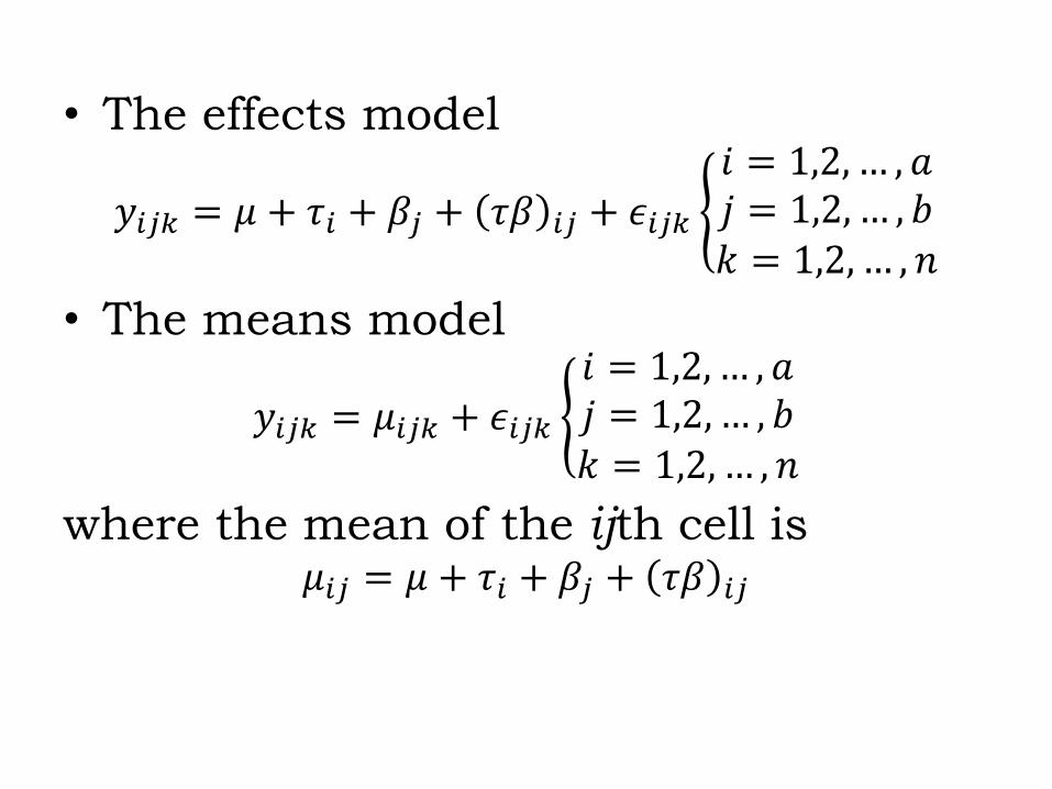
• The effects model
𝑦𝑖𝑗𝑘 = 𝜇 + 𝜏𝑖 + 𝛽𝑗 + 𝜏𝛽 𝑖𝑗 + 𝜖𝑖𝑗𝑘 𝑖 = 1,2, … , 𝑎𝑗 = 1,2, … , 𝑏𝑘 = 1,2, … , 𝑛
• The means model
𝑦𝑖𝑗𝑘 = 𝜇𝑖𝑗𝑘 + 𝜖𝑖𝑗𝑘 𝑖 = 1,2, … , 𝑎𝑗 = 1,2, … , 𝑏𝑘 = 1,2, … , 𝑛
where the mean of the ijth cell is 𝜇𝑖𝑗 = 𝜇 + 𝜏𝑖 + 𝛽𝑗 + 𝜏𝛽 𝑖𝑗
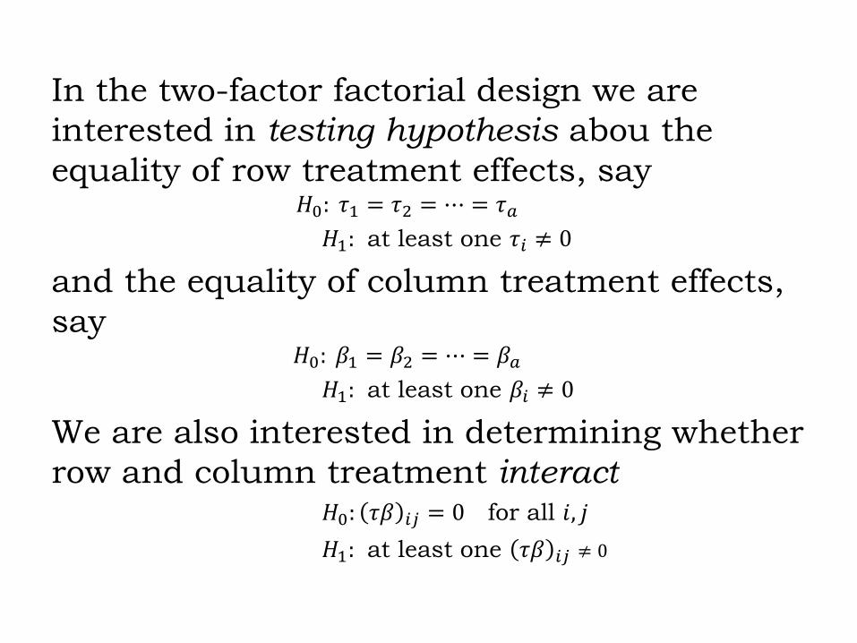
In the two-factor factorial design we are
interested in testing hypothesis abou the
equality of row treatment effects, say 𝐻0: 𝜏1 = 𝜏2 = ⋯ = 𝜏𝑎
𝐻1: at least one 𝜏𝑖 ≠ 0
and the equality of column treatment effects,
say 𝐻0: 𝛽1 = 𝛽2 = ⋯ = 𝛽𝑎
𝐻1: at least one 𝛽𝑖 ≠ 0
We are also interested in determining whether
row and column treatment interact 𝐻0: 𝜏𝛽 𝑖𝑗 = 0 for all 𝑖, 𝑗
𝐻1: at least one 𝜏𝛽 𝑖𝑗 ≠ 0
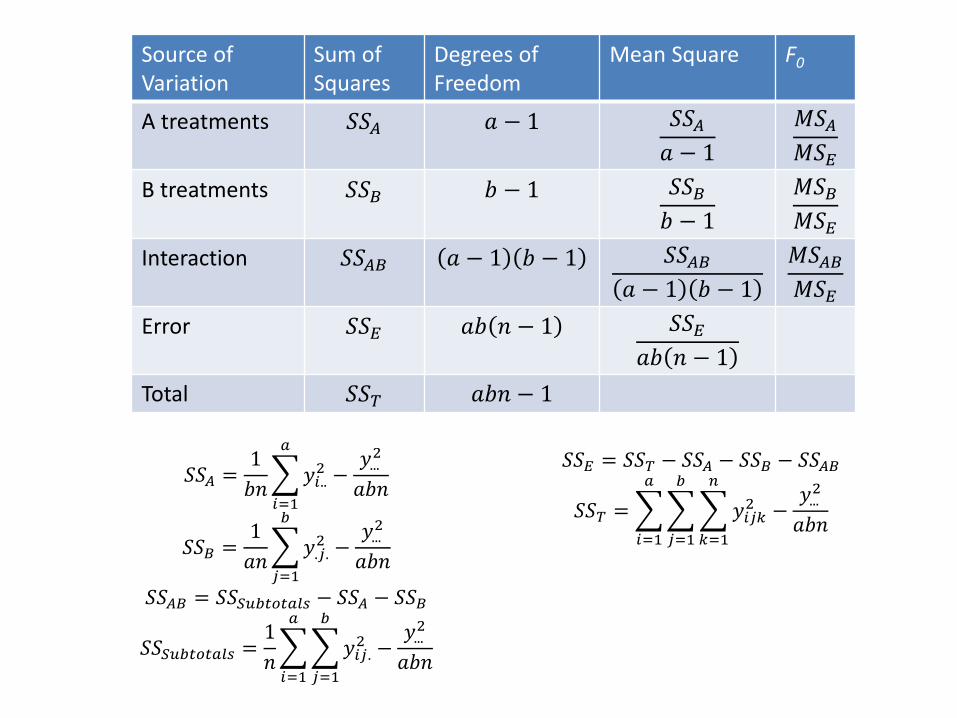
Source of Variation
Sum of Squares
Degrees of Freedom
Mean Square F0
A treatments 𝑆𝑆𝐴 𝑎 − 1 𝑆𝑆𝐴𝑎 − 1
𝑀𝑆𝐴𝑀𝑆𝐸
B treatments 𝑆𝑆𝐵 𝑏 − 1 𝑆𝑆𝐵
𝑏 − 1
𝑀𝑆𝐵
𝑀𝑆𝐸
Interaction 𝑆𝑆𝐴𝐵 𝑎 − 1 𝑏 − 1 𝑆𝑆𝐴𝐵
𝑎 − 1 𝑏 − 1
𝑀𝑆𝐴𝐵
𝑀𝑆𝐸
Error 𝑆𝑆𝐸 𝑎𝑏 𝑛 − 1 𝑆𝑆𝐸
𝑎𝑏 𝑛 − 1
Total 𝑆𝑆𝑇 𝑎𝑏𝑛 − 1
𝑆𝑆𝐴 =1
𝑏𝑛 𝑦𝑖..
2 −𝑦...
2
𝑎𝑏𝑛
𝑎
𝑖=1
𝑆𝑆𝐵 =1
𝑎𝑛 𝑦.𝑗.
2 −𝑦...
2
𝑎𝑏𝑛
𝑏
𝑗=1
𝑆𝑆𝐴𝐵 = 𝑆𝑆𝑆𝑢𝑏𝑡𝑜𝑡𝑎𝑙𝑠 − 𝑆𝑆𝐴 − 𝑆𝑆𝐵
𝑆𝑆𝑆𝑢𝑏𝑡𝑜𝑡𝑎𝑙𝑠 =1
𝑛 𝑦𝑖𝑗.
2 −𝑦...
2
𝑎𝑏𝑛
𝑏
𝑗=1
𝑎
𝑖=1
𝑆𝑆𝐸 = 𝑆𝑆𝑇 − 𝑆𝑆𝐴 − 𝑆𝑆𝐵 − 𝑆𝑆𝐴𝐵
𝑆𝑆𝑇 = 𝑦𝑖𝑗𝑘2
𝑛
𝑘=1
−𝑦...
2
𝑎𝑏𝑛
𝑏
𝑗=1
𝑎
𝑖=1
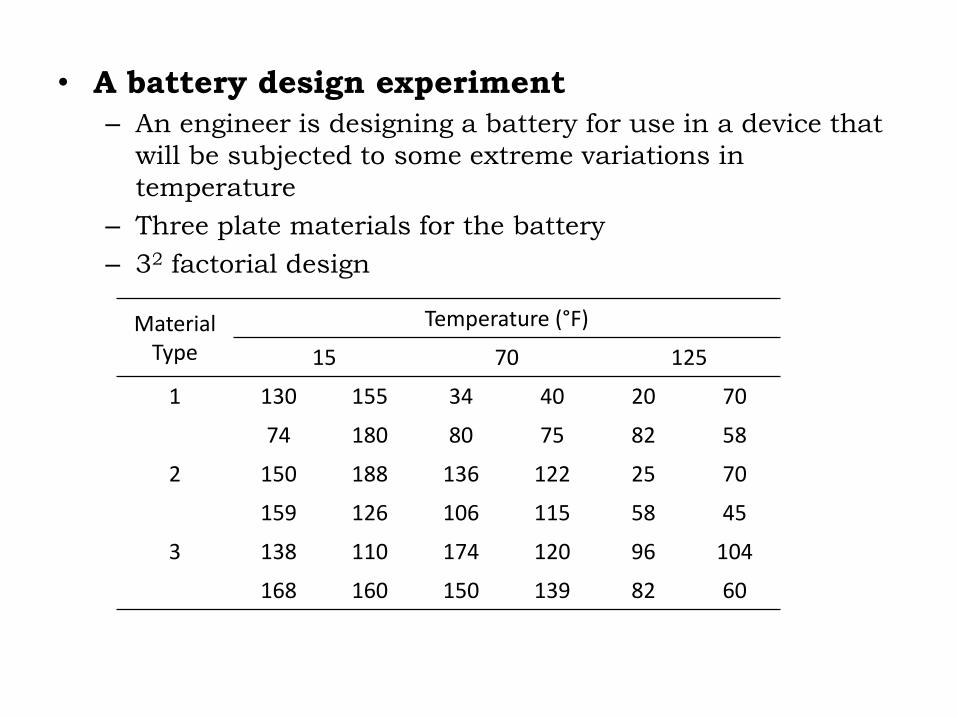
• A battery design experiment
– An engineer is designing a battery for use in a device that
will be subjected to some extreme variations in
temperature
– Three plate materials for the battery
– 32 factorial design
Material
Type
Temperature (°F)
15 70 125
1 130 155 34 40 20 70
74 180 80 75 82 58
2 150 188 136 122 25 70
159 126 106 115 58 45
3 138 110 174 120 96 104
168 160 150 139 82 60
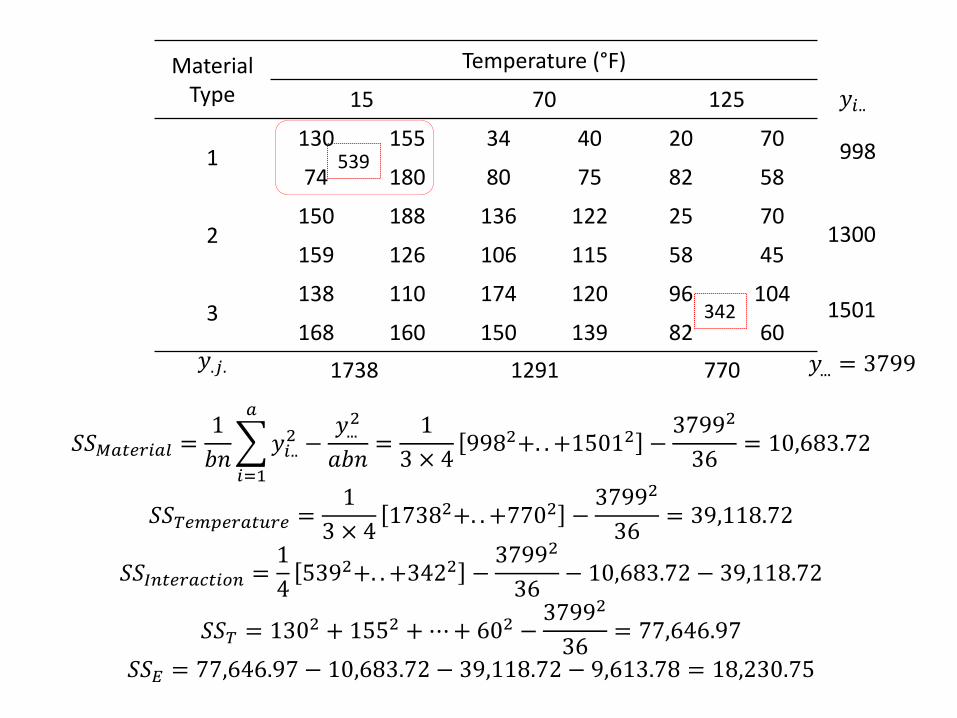
Material Type
Temperature (°F)
15 70 125
1 130 155 34 40 20 70
74 180 80 75 82 58
2 150 188 136 122 25 70
159 126 106 115 58 45
3 138 110 174 120 96 104
168 160 150 139 82 60
𝑆𝑆𝑀𝑎𝑡𝑒𝑟𝑖𝑎𝑙 =1
𝑏𝑛 𝑦𝑖..
2 −𝑦...
2
𝑎𝑏𝑛
𝑎
𝑖=1
=1
3 × 49982+. . +15012 −
37992
36= 10,683.72
𝑆𝑆𝑇𝑒𝑚𝑝𝑒𝑟𝑎𝑡𝑢𝑟𝑒 =1
3 × 417382+. . +7702 −
37992
36= 39,118.72
𝑆𝑆𝐼𝑛𝑡𝑒𝑟𝑎𝑐𝑡𝑖𝑜𝑛 =1
45392+. . +3422 −
37992
36− 10,683.72 − 39,118.72
𝑆𝑆𝑇 = 1302 + 1552 + ⋯+ 602 −37992
36= 77,646.97
𝑆𝑆𝐸 = 77,646.97 − 10,683.72 − 39,118.72 − 9,613.78 = 18,230.75
𝑦.𝑗. 1738 1291 770
998
1300
1501
𝑦𝑖..
𝑦... = 3799
539
342
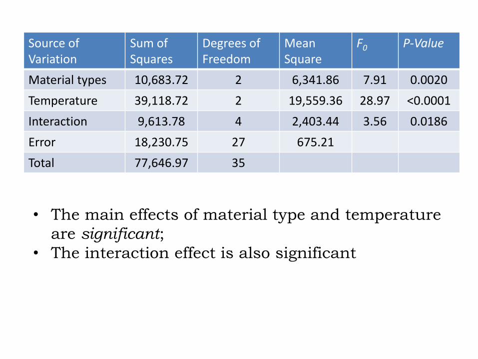
Source of Variation
Sum of Squares
Degrees of Freedom
Mean Square
F0 P-Value
Material types 10,683.72 2 6,341.86 7.91 0.0020
Temperature 39,118.72 2 19,559.36 28.97 <0.0001
Interaction 9,613.78 4 2,403.44 3.56 0.0186
Error 18,230.75 27 675.21
Total 77,646.97 35
• The main effects of material type and temperature
are significant;
• The interaction effect is also significant
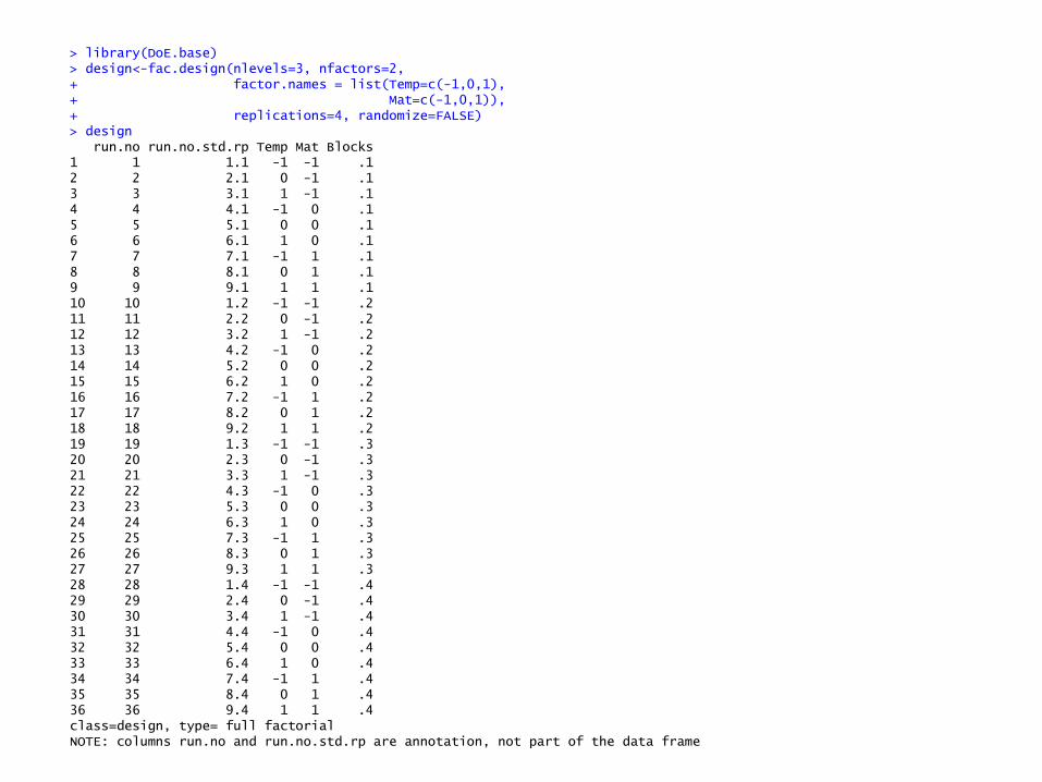
> library(DoE.base) > design<-fac.design(nlevels=3, nfactors=2, + factor.names = list(Temp=c(-1,0,1), + Mat=c(-1,0,1)), + replications=4, randomize=FALSE) > design run.no run.no.std.rp Temp Mat Blocks 1 1 1.1 -1 -1 .1 2 2 2.1 0 -1 .1 3 3 3.1 1 -1 .1 4 4 4.1 -1 0 .1 5 5 5.1 0 0 .1 6 6 6.1 1 0 .1 7 7 7.1 -1 1 .1 8 8 8.1 0 1 .1 9 9 9.1 1 1 .1 10 10 1.2 -1 -1 .2 11 11 2.2 0 -1 .2 12 12 3.2 1 -1 .2 13 13 4.2 -1 0 .2 14 14 5.2 0 0 .2 15 15 6.2 1 0 .2 16 16 7.2 -1 1 .2 17 17 8.2 0 1 .2 18 18 9.2 1 1 .2 19 19 1.3 -1 -1 .3 20 20 2.3 0 -1 .3 21 21 3.3 1 -1 .3 22 22 4.3 -1 0 .3 23 23 5.3 0 0 .3 24 24 6.3 1 0 .3 25 25 7.3 -1 1 .3 26 26 8.3 0 1 .3 27 27 9.3 1 1 .3 28 28 1.4 -1 -1 .4 29 29 2.4 0 -1 .4 30 30 3.4 1 -1 .4 31 31 4.4 -1 0 .4 32 32 5.4 0 0 .4 33 33 6.4 1 0 .4 34 34 7.4 -1 1 .4 35 35 8.4 0 1 .4 36 36 9.4 1 1 .4 class=design, type= full factorial NOTE: columns run.no and run.no.std.rp are annotation, not part of the data frame
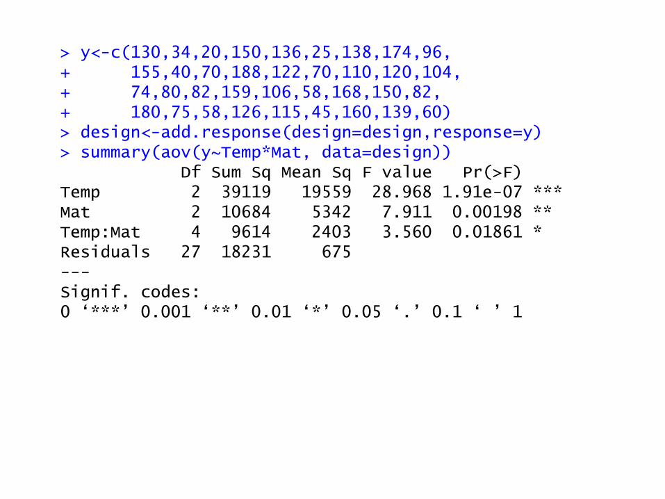
> y<-c(130,34,20,150,136,25,138,174,96, + 155,40,70,188,122,70,110,120,104, + 74,80,82,159,106,58,168,150,82, + 180,75,58,126,115,45,160,139,60) > design<-add.response(design=design,response=y) > summary(aov(y~Temp*Mat, data=design)) Df Sum Sq Mean Sq F value Pr(>F) Temp 2 39119 19559 28.968 1.91e-07 *** Mat 2 10684 5342 7.911 0.00198 ** Temp:Mat 4 9614 2403 3.560 0.01861 * Residuals 27 18231 675 --- Signif. codes: 0 ‘***’ 0.001 ‘**’ 0.01 ‘*’ 0.05 ‘.’ 0.1 ‘ ’ 1
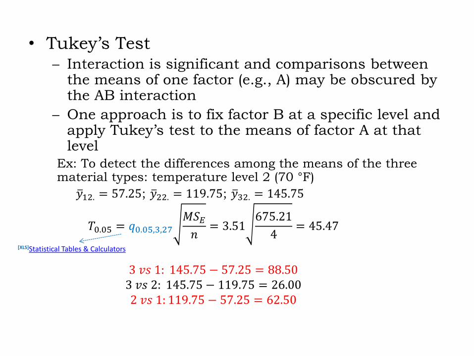
• Tukey’s Test – Interaction is significant and comparisons between
the means of one factor (e.g., A) may be obscured by the AB interaction
– One approach is to fix factor B at a specific level and apply Tukey’s test to the means of factor A at that level
Ex: To detect the differences among the means of the three material types: temperature level 2 (70 °F)
𝑦 12. = 57.25; 𝑦 22. = 119.75; 𝑦 32. = 145.75
𝑇0.05 = 𝑞0.05,3,27
𝑀𝑆𝐸
𝑛= 3.51
675.21
4= 45.47
3 𝑣𝑠 1: 145.75 − 57.25 = 88.50
3 𝑣𝑠 2: 145.75 − 119.75 = 26.00
2 𝑣𝑠 1: 119.75 − 57.25 = 62.50
[XLS]Statistical Tables & Calculators
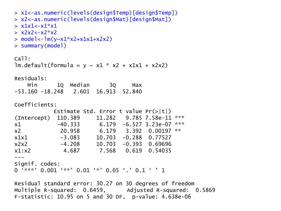
> x1<-as.numeric(levels(design$Temp)[design$Temp]) > x2<-as.numeric(levels(design$Mat)[design$Mat]) > x1x1<-x1*x1 > x2x2<-x2*x2 > model<-lm(y~x1*x2+x1x1+x2x2) > summary(model) Call: lm.default(formula = y ~ x1 * x2 + x1x1 + x2x2) Residuals: Min 1Q Median 3Q Max -53.160 -18.248 2.601 16.913 52.840 Coefficients: Estimate Std. Error t value Pr(>|t|) (Intercept) 110.389 11.282 9.785 7.58e-11 *** x1 -40.333 6.179 -6.527 3.23e-07 *** x2 20.958 6.179 3.392 0.00197 ** x1x1 -3.083 10.703 -0.288 0.77527 x2x2 -4.208 10.703 -0.393 0.69696 x1:x2 4.687 7.568 0.619 0.54035 --- Signif. codes: 0 ‘***’ 0.001 ‘**’ 0.01 ‘*’ 0.05 ‘.’ 0.1 ‘ ’ 1 Residual standard error: 30.27 on 30 degrees of freedom Multiple R-squared: 0.6459, Adjusted R-squared: 0.5869 F-statistic: 10.95 on 5 and 30 DF, p-value: 4.638e-06
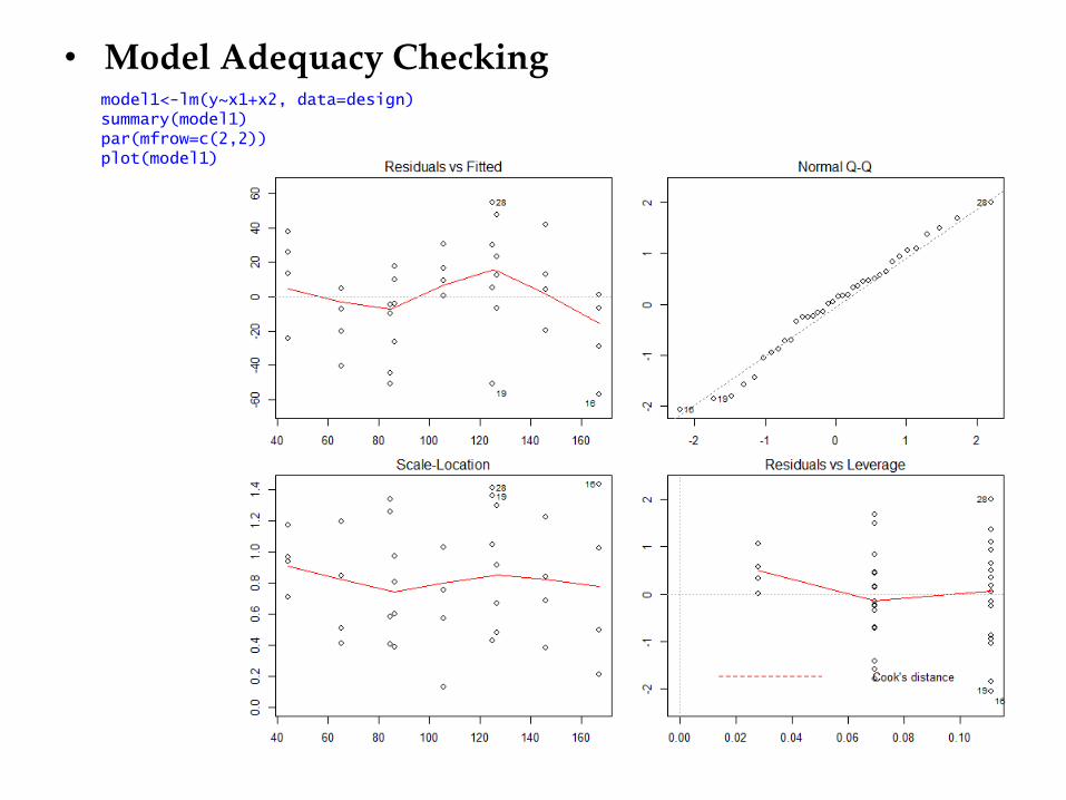
• Model Adequacy Checking
model1<-lm(y~x1+x2, data=design) summary(model1) par(mfrow=c(2,2)) plot(model1)
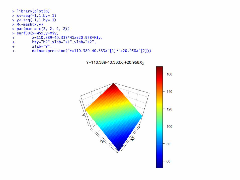
> library(plot3D) > x<-seq(-1,1,by=.1) > y<-seq(-1,1,by=.1) > M<-mesh(x,y) > par(mar = c(2, 2, 2, 2)) > surf3D(x=M$x,y=M$y, + z=110.389-40.333*M$x+20.958*M$y, + bty="b2",xlab="X1",ylab="X2", + zlab="Y", + main=expression("Y=110.389-40.333X"[1]*"+20.958X"[2]))
Montgomery, pg. 398
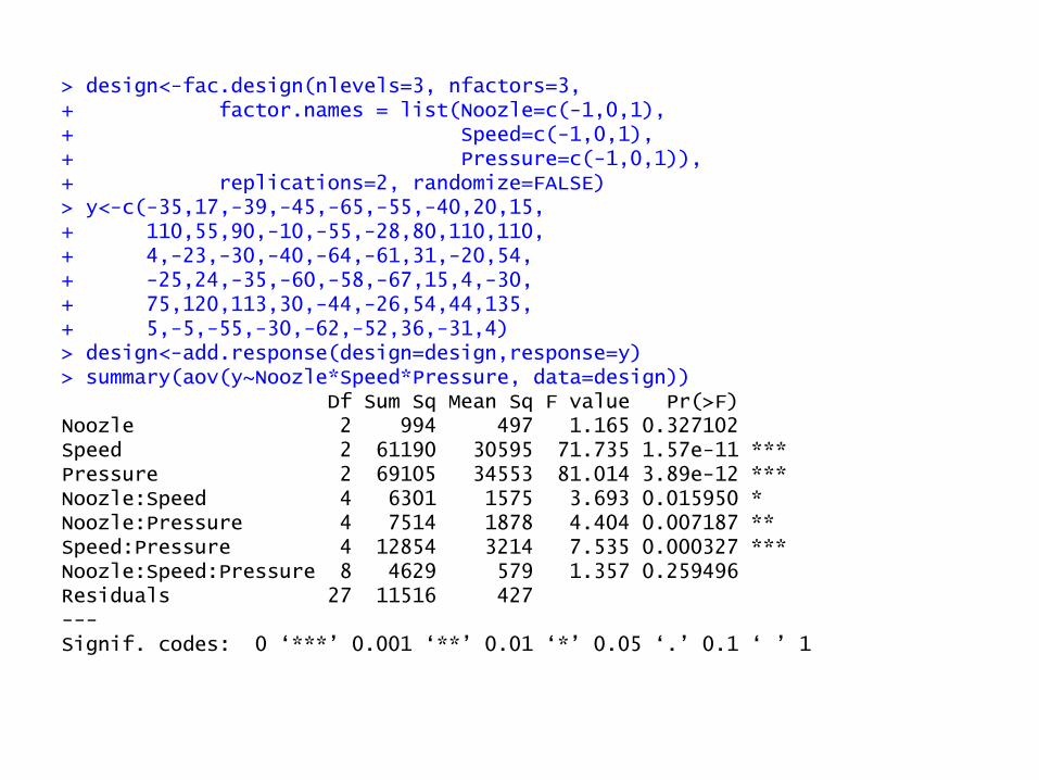
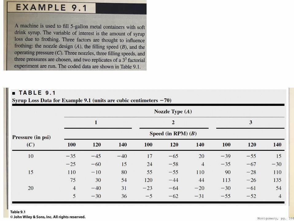
> design<-fac.design(nlevels=3, nfactors=3, + factor.names = list(Noozle=c(-1,0,1), + Speed=c(-1,0,1), + Pressure=c(-1,0,1)), + replications=2, randomize=FALSE) > y<-c(-35,17,-39,-45,-65,-55,-40,20,15, + 110,55,90,-10,-55,-28,80,110,110, + 4,-23,-30,-40,-64,-61,31,-20,54, + -25,24,-35,-60,-58,-67,15,4,-30, + 75,120,113,30,-44,-26,54,44,135, + 5,-5,-55,-30,-62,-52,36,-31,4) > design<-add.response(design=design,response=y) > summary(aov(y~Noozle*Speed*Pressure, data=design)) Df Sum Sq Mean Sq F value Pr(>F) Noozle 2 994 497 1.165 0.327102 Speed 2 61190 30595 71.735 1.57e-11 *** Pressure 2 69105 34553 81.014 3.89e-12 *** Noozle:Speed 4 6301 1575 3.693 0.015950 * Noozle:Pressure 4 7514 1878 4.404 0.007187 ** Speed:Pressure 4 12854 3214 7.535 0.000327 *** Noozle:Speed:Pressure 8 4629 579 1.357 0.259496 Residuals 27 11516 427 --- Signif. codes: 0 ‘***’ 0.001 ‘**’ 0.01 ‘*’ 0.05 ‘.’ 0.1 ‘ ’ 1
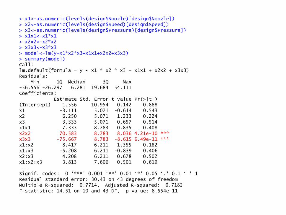
> x1<-as.numeric(levels(design$Noozle)[design$Noozle]) > x2<-as.numeric(levels(design$Speed)[design$Speed]) > x3<-as.numeric(levels(design$Pressure)[design$Pressure]) > x1x1<-x1*x1 > x2x2<-x2*x2 > x3x3<-x3*x3 > model<-lm(y~x1*x2*x3+x1x1+x2x2+x3x3) > summary(model) Call: lm.default(formula = y ~ x1 * x2 * x3 + x1x1 + x2x2 + x3x3) Residuals: Min 1Q Median 3Q Max -56.556 -26.297 6.281 19.684 54.111 Coefficients: Estimate Std. Error t value Pr(>|t|) (Intercept) 1.556 10.954 0.142 0.888 x1 -3.111 5.071 -0.614 0.543 x2 6.250 5.071 1.233 0.224 x3 3.333 5.071 0.657 0.514 x1x1 7.333 8.783 0.835 0.408 x2x2 70.583 8.783 8.036 4.21e-10 *** x3x3 -75.667 8.783 -8.615 6.49e-11 *** x1:x2 8.417 6.211 1.355 0.182 x1:x3 -5.208 6.211 -0.839 0.406 x2:x3 4.208 6.211 0.678 0.502 x1:x2:x3 3.813 7.606 0.501 0.619 --- Signif. codes: 0 ‘***’ 0.001 ‘**’ 0.01 ‘*’ 0.05 ‘.’ 0.1 ‘ ’ 1 Residual standard error: 30.43 on 43 degrees of freedom Multiple R-squared: 0.7714, Adjusted R-squared: 0.7182 F-statistic: 14.51 on 10 and 43 DF, p-value: 8.554e-11
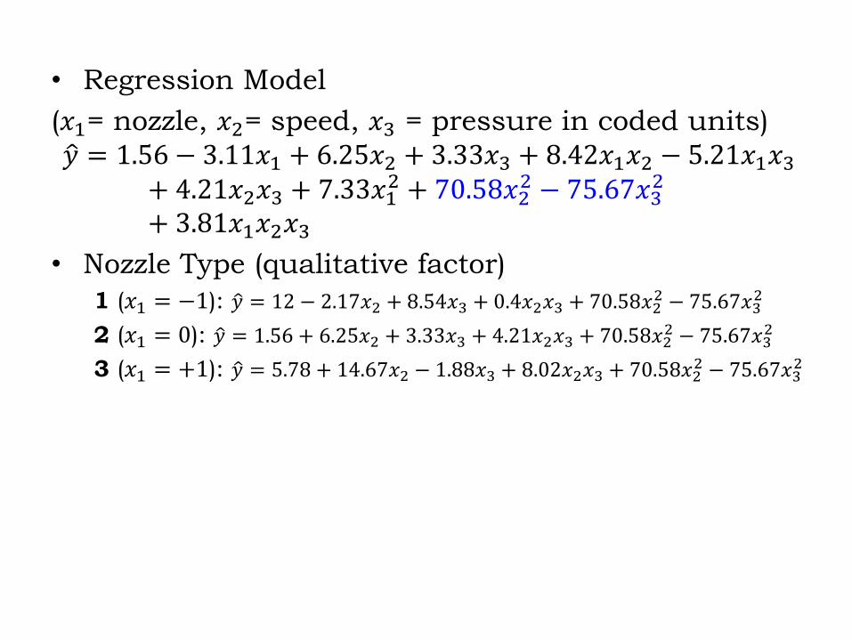
• Regression Model
(𝑥1= nozzle, 𝑥2= speed, 𝑥3 = pressure in coded units)
𝑦 = 1.56 − 3.11𝑥1 + 6.25𝑥2 + 3.33𝑥3 + 8.42𝑥1𝑥2 − 5.21𝑥1𝑥3
+ 4.21𝑥2𝑥3 + 7.33𝑥12 + 70.58𝑥2
2 − 75.67𝑥32
+ 3.81𝑥1𝑥2𝑥3
• Nozzle Type (qualitative factor)
1 (𝑥1 = −1): 𝑦 = 12 − 2.17𝑥2 + 8.54𝑥3 + 0.4𝑥2𝑥3 + 70.58𝑥22 − 75.67𝑥3
2
2 (𝑥1 = 0): 𝑦 = 1.56 + 6.25𝑥2 + 3.33𝑥3 + 4.21𝑥2𝑥3 + 70.58𝑥22 − 75.67𝑥3
2
3 (𝑥1 = +1): 𝑦 = 5.78 + 14.67𝑥2 − 1.88𝑥3 + 8.02𝑥2𝑥3 + 70.58𝑥22 − 75.67𝑥3
2
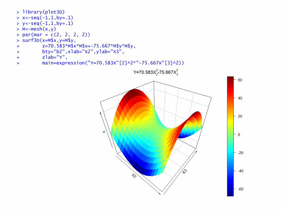
> library(plot3D) > x<-seq(-1,1,by=.1) > y<-seq(-1,1,by=.1) > M<-mesh(x,y) > par(mar = c(2, 2, 2, 2)) > surf3D(x=M$x,y=M$y, + z=70.583*M$x*M$x+-75.667*M$y*M$y, + bty="b2",xlab="X2",ylab="X3", + zlab="Y", + main=expression("Y=70.583X"[2]^2*"-75.667X"[3]^2))
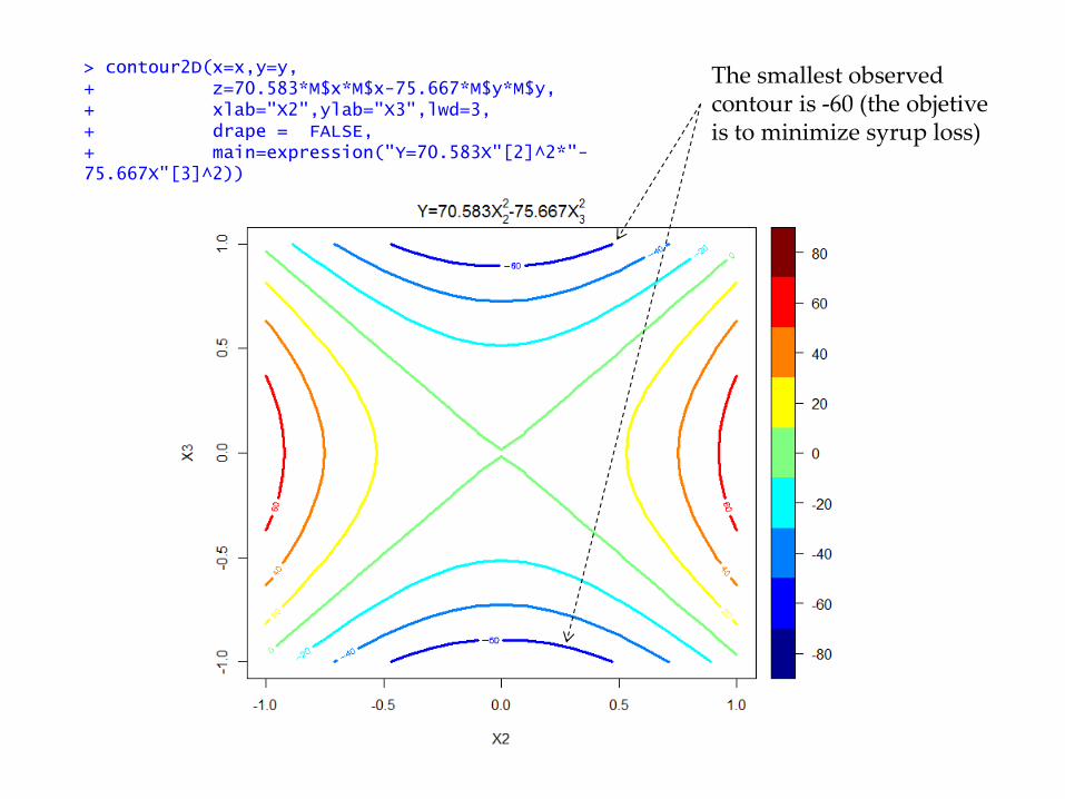
> contour2D(x=x,y=y, + z=70.583*M$x*M$x-75.667*M$y*M$y, + xlab="X2",ylab="X3",lwd=3, + drape = FALSE, + main=expression("Y=70.583X"[2]^2*"-75.667X"[3]^2))
The smallest observed contour is -60 (the objetive is to minimize syrup loss)
Factorial with Mixed Levels
• Two-level factorial and fractional designs
are of great practical importance
• The three-level system is much less useful
because the designs are relatively large even
for a modest number of factors
• In some situations it is necessary to include
a factor (or a few factors) that has more
than two levels
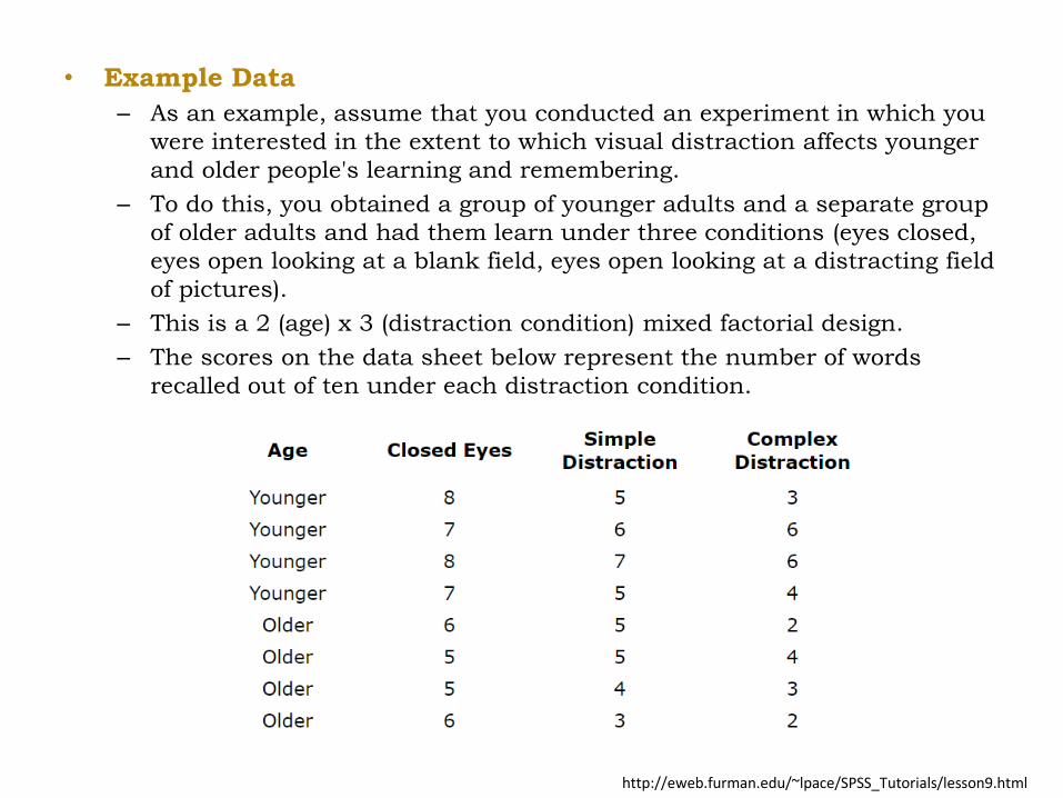
• Example Data
– As an example, assume that you conducted an experiment in which you
were interested in the extent to which visual distraction affects younger
and older people's learning and remembering.
– To do this, you obtained a group of younger adults and a separate group
of older adults and had them learn under three conditions (eyes closed,
eyes open looking at a blank field, eyes open looking at a distracting field
of pictures).
– This is a 2 (age) x 3 (distraction condition) mixed factorial design.
– The scores on the data sheet below represent the number of words
recalled out of ten under each distraction condition.
http://eweb.furman.edu/~lpace/SPSS_Tutorials/lesson9.html

> design2x3 <- regular.design(factors=list(Age=1:2,Distraction=1:3), + model=~Age*Distraction, + nunits=24) > print(design2x3@design) Age Distraction 1 1 1 2 1 2 3 1 3 4 1 1 5 1 2 6 1 3 7 1 1 8 1 2 9 1 3 10 1 1 11 1 2 12 1 3 13 2 1 14 2 2 15 2 3 16 2 1 17 2 2 18 2 3 19 2 1 20 2 2 21 2 3 22 2 1 23 2 2 24 2 3
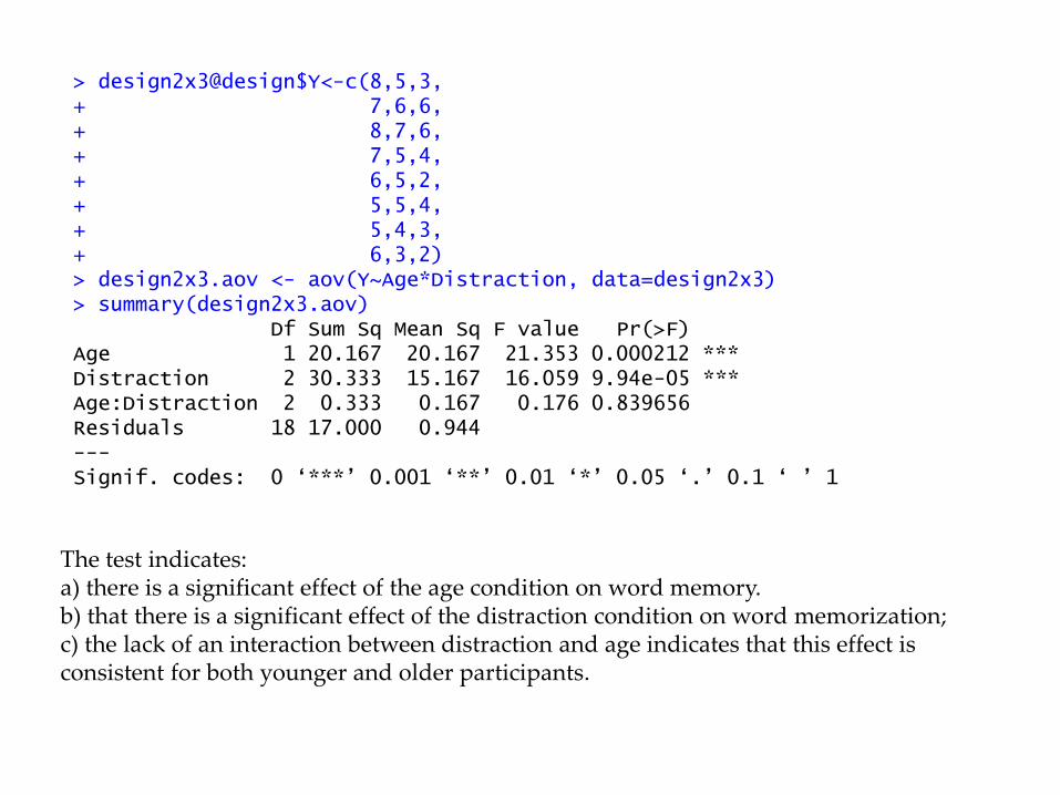
> design2x3@design$Y<-c(8,5,3, + 7,6,6, + 8,7,6, + 7,5,4, + 6,5,2, + 5,5,4, + 5,4,3, + 6,3,2) > design2x3.aov <- aov(Y~Age*Distraction, data=design2x3) > summary(design2x3.aov) Df Sum Sq Mean Sq F value Pr(>F) Age 1 20.167 20.167 21.353 0.000212 *** Distraction 2 30.333 15.167 16.059 9.94e-05 *** Age:Distraction 2 0.333 0.167 0.176 0.839656 Residuals 18 17.000 0.944 --- Signif. codes: 0 ‘***’ 0.001 ‘**’ 0.01 ‘*’ 0.05 ‘.’ 0.1 ‘ ’ 1
The test indicates: a) there is a significant effect of the age condition on word memory. b) that there is a significant effect of the distraction condition on word memorization; c) the lack of an interaction between distraction and age indicates that this effect is consistent for both younger and older participants.
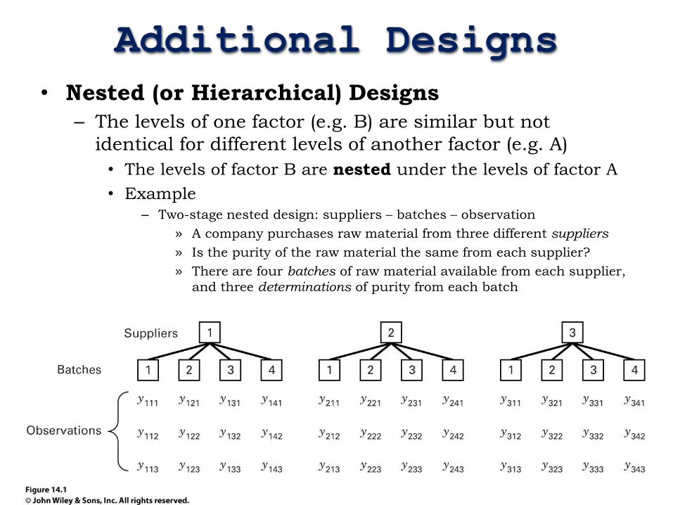
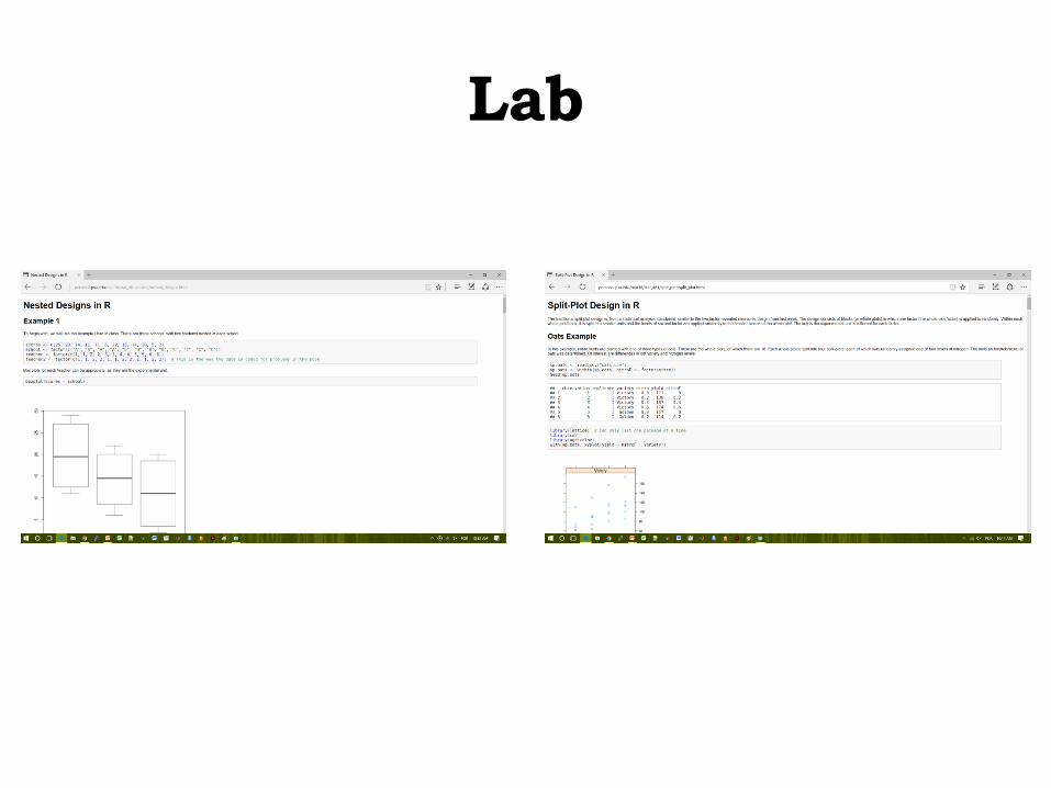
Additional Designs
• Nested (or Hierarchical) Designs
– The levels of one factor (e.g. B) are similar but not
identical for different levels of another factor (e.g. A)
• The levels of factor B are nested under the levels of factor A
• Example – Two-stage nested design: suppliers – batches – observation
» A company purchases raw material from three different suppliers
» Is the purity of the raw material the same from each supplier?
» There are four batches of raw material available from each supplier,
and three determinations of purity from each batch
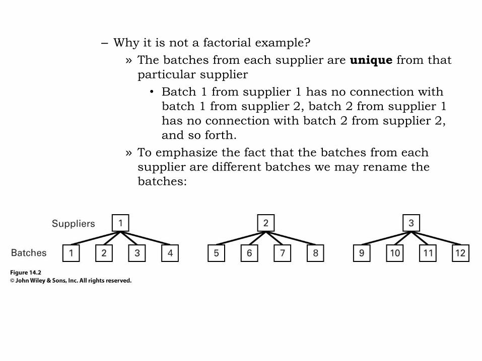
– Why it is not a factorial example?
» The batches from each supplier are unique from that
particular supplier
• Batch 1 from supplier 1 has no connection with
batch 1 from supplier 2, batch 2 from supplier 1
has no connection with batch 2 from supplier 2,
and so forth.
» To emphasize the fact that the batches from each
supplier are different batches we may rename the
batches:
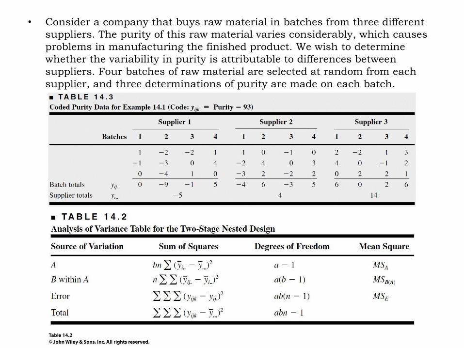
• Consider a company that buys raw material in batches from three different
suppliers. The purity of this raw material varies considerably, which causes
problems in manufacturing the finished product. We wish to determine
whether the variability in purity is attributable to differences between
suppliers. Four batches of raw material are selected at random from each
supplier, and three determinations of purity are made on each batch.
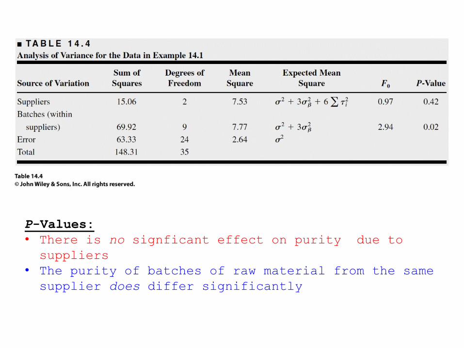
P-Values:
• There is no signficant effect on purity due to
suppliers
• The purity of batches of raw material from the same
supplier does differ significantly
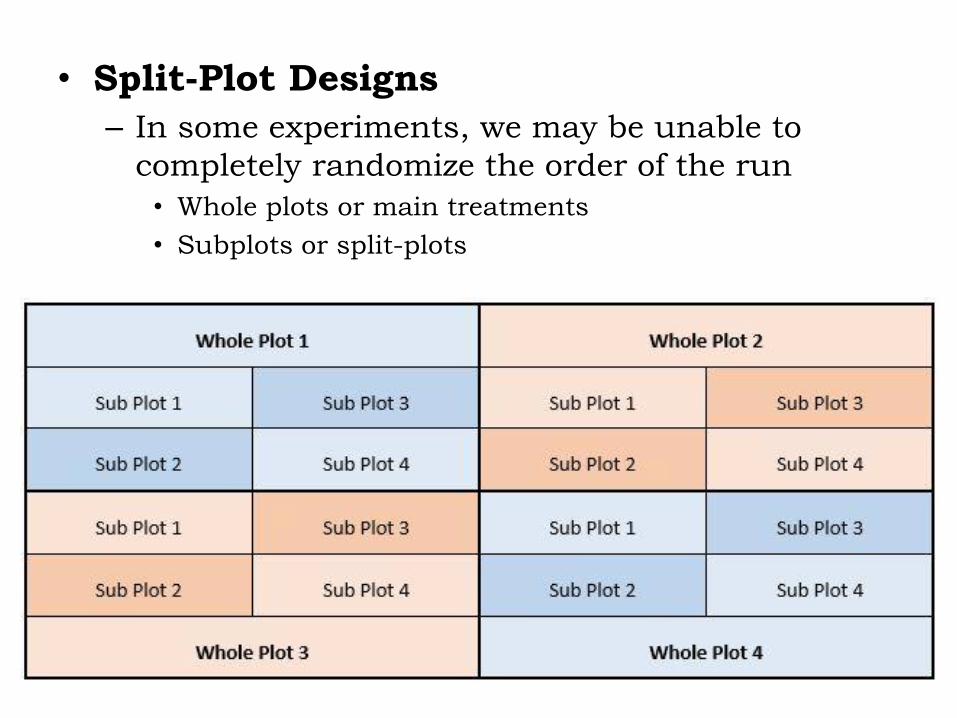
• Split-Plot Designs
– In some experiments, we may be unable to
completely randomize the order of the run
• Whole plots or main treatments
• Subplots or split-plots
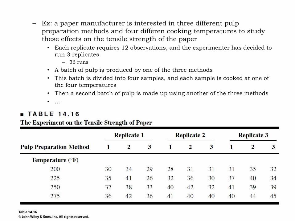
– Ex: a paper manufacturer is interested in three different pulp
preparation methods and four differen cooking temperatures to study
these effects on the tensile strength of the paper
• Each replicate requires 12 observations, and the experimenter has decided to
run 3 replicates
– 36 runs
• A batch of pulp is produced by one of the three methods
• This batch is divided into four samples, and each sample is cooked at one of
the four temperatures
• Then a second batch of pulp is made up using another of the three methods
• ...
– Why it is not a factorial example (three levels of
preparation method, factor A, four levels of temperature,
factor B)?
• If this is the case, then the order of the experimentation within each
replicate should be completely randomized – Treatment combinations (preparation method and temperature) should be randomly
selected
• But, the experimenter did no collect the data this way – He made up a batch of pulp and obtained observations for all temperatures from that
batch
– The only feasible way to run this experiment: preparing the bathes (economics) and
the size of the batches
– A completely randomized factorial experiment: 36 batches of
pulp
– Split-plot design: 9 batches total
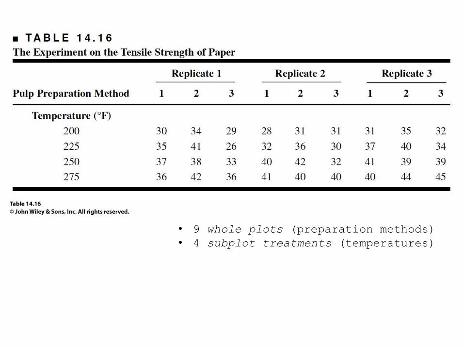
• 9 whole plots (preparation methods)
• 4 subplot treatments (temperatures)
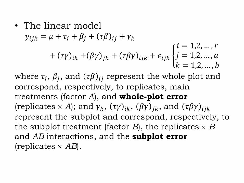
• The linear model 𝑦𝑖𝑗𝑘 = 𝜇 + 𝜏𝑖 + 𝛽𝑗 + 𝜏𝛽 𝑖𝑗 + 𝛾𝑘
+ 𝜏𝛾 𝑖𝑘 + 𝛽𝛾 𝑗𝑘 + 𝜏𝛽𝛾 𝑖𝑗𝑘 + 𝜖𝑖𝑗𝑘 𝑖 = 1,2,… , 𝑟𝑗 = 1,2,… , 𝑎𝑘 = 1,2,… , 𝑏
where 𝜏𝑖, 𝛽𝑗, and 𝜏𝛽 𝑖𝑗 represent the whole plot and
correspond, respectively, to replicates, main
treatments (factor A), and whole-plot error
(replicates A); and 𝛾𝑘, 𝜏𝛾 𝑖𝑘, 𝛽𝛾 𝑗𝑘, and 𝜏𝛽𝛾 𝑖𝑗𝑘
represent the subplot and correspond, respectively, to
the subplot treatment (factor B), the replicates B
and AB interactions, and the subplot error
(replicates AB).

The split-plot design has an agricultural heritage
• Whole plots: large areas of land
• Subplots: smaller areas of land within large areas
• Ex: several varieties of a crop could be planted in different
fields (whole plots), one variety to a field
– Each field could be divided into, say, four subplots, and each
subplot could be treated with different type os fertilizer.
– Here the crop varietes are the main treatments and the different
fertilizers are the subtreatments.