Procedia Materials Science 10 ( 2015 ) 768 – 788

Available online at www.sciencedirect.com

2211-8128 © 2015 The Authors. Published by Elsevier Ltd. This is an open access article under the CC BY-NC-ND license (http://creativecommons.org/licenses/by-nc-nd/4.0/).Peer-review under responsibility of the International Conference on Nanomaterials and Technologies (CNT 2014)doi: 10.1016/j.mspro.2015.06.022

ScienceDirect

*Coorespong author:srinivasakarumuri@gmail.com; 2211-8128 © 2015 The Authors. Published by Elsevier Ltd.

2nd International Conference on Nanomaterials and Technologies (CNT 2014)

Design and analysis of fluid structure interaction in a horizontal Micro Channel

K.Srinivasa Raoa*, K.Girija Sravanib, G.Yugandharc,G.Venkateswara Raod and V.N.Manie

aDepartment of ECE, KL University, Green Fields, Vaddeswaram-522502, Guntur, A.P, India

bDepartment of ECE, Amrita Sai Institute of Technology and Sciences, A.P, India cDepartment of Computer Science Engineering, GITAM University, Hyderabad-502329, Telangana, India

dDepartment of Information Technology, GITAM University, Vishakhapatnam, 530045,A.P India eDepartment of Electronics, Centre for Materials for Electronics Technology(C-MET), Hyderabad, A.P, India.

Abstract

This paper demonstrates techniques for modelling fluid-structure interactions using COMSOL Multiphysics v 4.2a, which illustrates how to solve for the flow in a continuously deforming geometry using the Arbitrary Lagrangian-Eulerian (ALE) technique and corresponding deformation, displacement analysis. The present work reports the computation of the deformation and displacement in structure along with the fluid flow in a continuously deforming geometry, for different types of structures like circular, rectangular, ellipse, which are placed inside of the flow channel as an obstacle. Fluid structure interaction between wind and sails, modelling of parachutes, fluid structure thermal calculation, stability and response of aircraft wings, the flow of blood through arteries, response of bridges and tall buildings to winds, prediction of aero elastic parameters in military aircrafts, vibration of turbine and compressor blades and the oscillation of heat exchangers can also be analysed using this method

© 2015 The Authors. Published by Elsevier Ltd. Peer-review under responsibility of the International Conference on Nanomaterials and Technologies (CNT 2014).

Keywords: MEMS flow channel, structural interaction, COMSOL

1. Introduction

In the recent years, there has been rapid progress in the manufacturing of microfluidic devices used for various aspects of engineering and bio-medical purposes. Microfluidics refers to a set of technologies that control the flow of minute amounts of liquids or gases, typically measured in nano- and picoliters, in a miniaturized system and microfluidic devices are characterized by micro-channels having dimensions in the micrometer ( m) region. The most mature application of Microfluidics technology is in the commonly used inkjet printer which uses orifices

© 2015 The Authors. Published by Elsevier Ltd. This is an open access article under the CC BY-NC-ND license (http://creativecommons.org/licenses/by-nc-nd/4.0/).Peer-review under responsibility of the International Conference on Nanomaterials and Technologies (CNT 2014)

769 K. Srinivasa Rao et al. / Procedia Materials Science 10 ( 2015 ) 768 – 788

less than 100 m in diameter to generate ink droplets. Microfluidic devices have over the years moved to applications in biotechnology such as the development of DNA chips and lab-on-a-chip technology where they are being used to detect bacteria, viruses and cancer cells and having many advantages as compared to conventional analysis. Some of these advantages are lower fluid consumption, better process control, higher analysis speed and a lower fabrication cost; all of which reduce cost and time and are beneficial to present and future patients. Microfluidic devices however are not just scaled down versions of conventional testing equipment as the physics changes at the micro-scale level. As the dimensions of a microfluidic device are small, particles suspended in a fluid become comparable in size to the device itself, which dramatically alters system behavior. Although the fluid properties remain the same as that at the micro scale, some properties such as surface tension, viscosity, and electrical charges can become dominant forces on a fluid because the surface-to-volume ratio is much greater than for macro-scale systems. Therefore the stresses and strains which act on biological cells as they flow through a microdevice can be quite different and more complex than through conventional lab equipment. Stresses and strains have been known to produce certain biological and biochemical responses in cells leading to events such as spontaneous cell movement, cell differentiation and even cell death. Hence, the study of forces acting on cells in microfluidic devices through the fluid medium and the resulting deformation is an important first step towards a quantitative study in the change of physical properties of cells or biomolecules which pass through microfluidic devices [1]. Another area of interest is in the trajectories of the cells as they pass through the microchannel as this has implications on cell sorting techniques whereby cells are sorted by size or other parameters through fluorescent excitation. As the field of microfluidics is relatively new, numerical simulations of microfluidic systems are helpful in providing a research tool. By incorporating the complexities of channel and cell geometry, fluid flow patterns as well as the structural mechanics of cells into a numerical model, the behavior of a system can be accurately predicted when an intuitive prediction may be difficult or impossible to be proven via mathematical methods. Numerical modeling also allows visualization of complex flow phenomena that will result due to fluid structure interactions that may not be easily obtained experimentally due to the minute dimensional nature of the system. The weakness of numerical modeling is the fact that it is not guaranteed to exactly replicate events in nature, particularly if there are physical phenomena that are not considered and incorporated into the model.

Fluid-structure interaction problems, as well as many other multi-field problems, have received much attention in recent years and their importance is still continuously growing. The main reason for this is that they are of great relevance in all fields of engineering (aerospace, bio, civil, mechanical, etc.) as well as in the applied sciences. Hence, the development and application of respective modelling and simulation approaches have gained great attention over the past decades. While modelling and simulation of most relevant problems were far out of reach still a couple of years ago, this possibility is now available or only a short distance away– thanks to advances in computational power, computational modelling approaches and methods. Many numerical structural models have been developed to describe the behaviour of structural interaction with the flowing fluid. The Fluid-Structure Interaction (FSI) multiphysics interface combines fluid flow with solid mechanics to capture the interaction between the fluid and the solid structure. A Solid Mechanics interface and a Single-Phase Flow interface model the solid and the fluid, respectively. The FSI couplings appear on the boundaries between the fluid and the solid. The Fluid-Structure Interaction interface uses an arbitrary Lagrangian-Eulerian (ALE) method to combine the fluid flow formulated using an Eulerian description and a spatial frame with solid mechanics formulated using a Lagrangian description and a material (reference) frame. The present work reports the analysis of the deformations made in the micro fluid channel by placing an obstructer, for various inlet mean velocities. Analysis of the displacements for various geometries was done i.e., by changing the shape to circle, ellipse etc., in which the pressure distribution is also observed. Changes in flow are observed after the deformation.

770 K. Srinivasa Rao et al. / Procedia Materials Science 10 ( 2015 ) 768 – 788

2. Theoretical background

The numerical simulation of multidimensional problems in fluid dynamics and nonlinear solid mechanics often requires coping with strong distortions of the continuum under consideration while allowing for a clear delineation of free surfaces and fluid–fluid, solid–solid, or fluid–structure interfaces. A fundamentally important consideration when developing a computer code for simulating problems in this class is the choice of an appropriate kinematical description of the continuum. In fact, such a choice determines the relationship between the deforming continuum and the finite grid or meshes of computing zones, and thus conditions the ability of the numerical method to deal with large distortions and provide an accurate resolution of material interfaces and mobile boundaries. An arbitrary Lagrangian-Eulerian (ALE) approach is used to derive the equations onthe deformable domain. So the structural deformations are solved using the elastic formulation and a nonlinear geometry formulation, which allow large deformations. Arbitrary Lagrangian Eulerian (ALE) frames is an approach to solving problems in engineering which combines the use of the classical Lagrangian and Eulerian reference frames. It is used largely in the analysis of fluid-structure interaction systems and is very helpful when analyzing structural motions in which the structure is severely deformed, such as an impact problem or the analysis of a very flexible structure. The Lagrangian Reference Frame is largely used in solid mechanics. It sets up a reference frame by fixing a grid to the material of interest and as the material deforms, the grid deforms with it. In this method, conservation of mass isautomatically satisfied because the individual sections of the grid always contain the same amount of mass. For structure motions with large deformation in which the grid becomes excessively distorted, the integration time steps become smaller and smaller because they are based on the size of the smallest section of the grid.

The Eulerian Reference Frame, which is fixed in space, is the typical frame work used in the analysis of fluid mechanics problems. In motion predictions solved through the Eulerian approach, the solution is generally measured in the net flow through a certain area and conservation of mass is taken into account explicitly by measuring the flux in and out of each grid section. The arbitrary Lagrangian-Eulerian (ALE) approach combines the use of the two reference frames. It allows for both a flexible grid and a grid that allows for material to flow through it. In essence, it takes the best part of both reference frames and combines them in to one. This is helpful in problems with large deformations in solid mechanics and in fluid-structure interaction. It allows for the grid to track the material to some extent, but when the grid deforms excessively and distorts the aspect ratio of the grid beyond an acceptable point it adjusts the grid and measures the flux of the material during the adjustment of the grid. The difficulty when using the ALE approach is deciding how much to allow a grid to deform and how much flux to allow. This is usually done by setting a limit on the distortion of a segment of a grid and once it deforms past that limit then that part of the grid is remeshed. Nonetheless, the use of the ALE may lead to failure when the mesh is deformed over certain limits and results in inverted coordinates. Inverted coordinates do not denote the failure of the entire model but implies that that results are these points cannot and will not be used in further iterations. As long as these points are not in the vicinity of the area of interest, the model can be still assumed to be reliable. Nevertheless, if there is a huge number of such inverted coordinates the accuracy of the solution deteriorates and eventually, the solution will cease to converge.

3. Use of COMSOL Multiphysics

The software package selected to model and simulate the MEMS based structural interactions with fluid flow was COMSOL Multiphysics Version 4.2 a. It is a powerful interactive environment for modelling and Multiphysics were selected because there was previous experience and expertise regarding its use as well as confidence in its capabilities. A finite element method based commercial software package, COMSOL Multiphysics, is used to produce a model and study the flow of liquid in the channel. Certain characteristics of COMSOL become

771 K. Srinivasa Rao et al. / Procedia Materials Science 10 ( 2015 ) 768 – 788

apparent with use. Compatibility stands out among these. COMSOL requires that every type of simulation included in the package has the ability to be combined with any other. This strict requirement actually mirrors what happens in the real world. The software has unique capabilities for solving the microfluidic model and fluid flow phenomena for real-world applications. The program provides an integrated geometry and graphical user interface for preparing the model, a computational solver for performing the simulation, and an interactive visualization program. COMSOL platform is adaptability. As your modeling needs change, so does the software. If you find yourself in need of including another physical effect, you can just add it. If one of the inputs to your model requires a formula, you can just enter it. Using tools like parameterized geometry, interactive meshing, and custom solver sequences, you can quickly adapt to the ebbs and flows of your requirements. This software provides the flexibility for selecting the required module using the model library, which consists of COMSOL Multiphysics, MEMS module, Microfluidics module, particle tracing module along with the live links for the MATLAB. This advanced version of software helps in designing the required geometry using free hand and the model can be analyzed form multiple angles as it provides the rotation flexibility while working with.

4. Design and Simulation of the Device

The design of the MEMS based structure includes defining the variables for the required geometry and

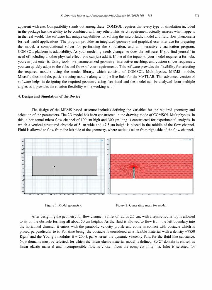
selection of the parameters. The 2D model has been constructed in the drawing mode of COMSOL Multiphysics. In this, a horizontal micro flow channel of 100 m high and 300 m long is constructed for experimental analysis, in which a vertical structured obstacle of 5 m wide and 47.5 m height is placed in the middle of the flow channel. Fluid is allowed to flow from the left side of the geometry, where outlet is taken from right side of the flow channel.

Figure 1: Model geometry. Figure 2: Generating mesh for model.

After designing the geometry for flow channel, a fillet of radius 2.5 m, with a semi-circular top is allowed

to sit on the obstacle forming all about 50 m heights. As the fluid is allowed to flow from the left boundary into the horizontal channel, it enters with the parabolic velocity profile and come in contact with obstacle which is placed perpendicular to it. For time being, the obstacle is considered as a flexible material with a density =7850 Kg/m3 and the Young’s modulus E = 200 k pa, whereas the dynamic viscosity Pa.s. for the fluid like substance. Now domains must be selected, for which the linear elastic material model is defined. So 2nd domain is chosen as linear elastic material and incompressible flow is chosen from the compressibility list. Inlet is selected for

772 K. Srinivasa Rao et al. / Procedia Materials Science 10 ( 2015 ) 768 – 788

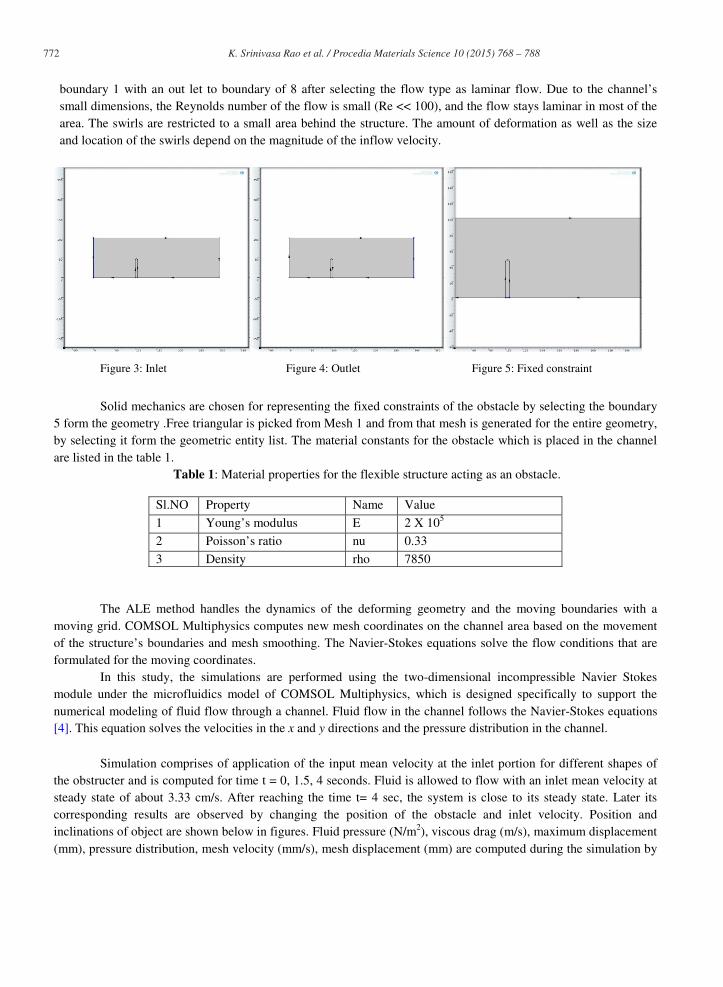
boundary 1 with an out let to boundary of 8 after selecting the flow type as laminar flow. Due to the channel’s small dimensions, the Reynolds number of the flow is small (Re << 100), and the flow stays laminar in most of the area. The swirls are restricted to a small area behind the structure. The amount of deformation as well as the size and location of the swirls depend on the magnitude of the inflow velocity.

Figure 3: Inlet Figure 4: Outlet Figure 5: Fixed constraint

Solid mechanics are chosen for representing the fixed constraints of the obstacle by selecting the boundary

5 form the geometry .Free triangular is picked from Mesh 1 and from that mesh is generated for the entire geometry, by selecting it form the geometric entity list. The material constants for the obstacle which is placed in the channel are listed in the table 1.

Table 1: Material properties for the flexible structure acting as an obstacle.

Sl.NO Property Name Value

1 Young’s modulus E 2 X 105

2 Poisson’s ratio nu 0.33

3 Density rho 7850

The ALE method handles the dynamics of the deforming geometry and the moving boundaries with a

moving grid. COMSOL Multiphysics computes new mesh coordinates on the channel area based on the movement of the structure’s boundaries and mesh smoothing. The Navier-Stokes equations solve the flow conditions that are formulated for the moving coordinates.

In this study, the simulations are performed using the two-dimensional incompressible Navier Stokes module under the microfluidics model of COMSOL Multiphysics, which is designed specifically to support the numerical modeling of fluid flow through a channel. Fluid flow in the channel follows the Navier-Stokes equations [4]. This equation solves the velocities in the x and y directions and the pressure distribution in the channel.

Simulation comprises of application of the input mean velocity at the inlet portion for different shapes of the obstructer and is computed for time t = 0, 1.5, 4 seconds. Fluid is allowed to flow with an inlet mean velocity at steady state of about 3.33 cm/s. After reaching the time t= 4 sec, the system is close to its steady state. Later its corresponding results are observed by changing the position of the obstacle and inlet velocity. Position and inclinations of object are shown below in figures. Fluid pressure (N/m2), viscous drag (m/s), maximum displacement (mm), pressure distribution, mesh velocity (mm/s), mesh displacement (mm) are computed during the simulation by

773 K. Srinivasa Rao et al. / Procedia Materials Science 10 ( 2015 ) 768 – 788

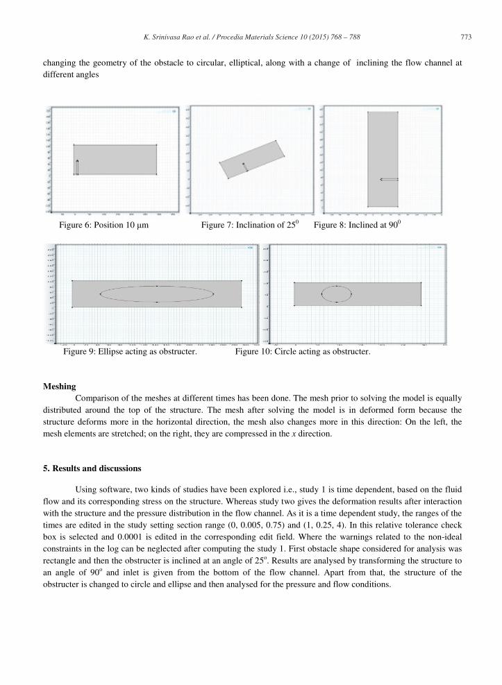
changing the geometry of the obstacle to circular, elliptical, along with a change of inclining the flow channel at different angles

Figure 6: Position 10 m Figure 7: Inclination of 250 Figure 8: Inclined at 900

Figure 9: Ellipse acting as obstructer. Figure 10: Circle acting as obstructer.

Meshing Comparison of the meshes at different times has been done. The mesh prior to solving the model is equally

distributed around the top of the structure. The mesh after solving the model is in deformed form because the structure deforms more in the horizontal direction, the mesh also changes more in this direction: On the left, the mesh elements are stretched; on the right, they are compressed in the x direction.

5. Results and discussions

Using software, two kinds of studies have been explored i.e., study 1 is time dependent, based on the fluid flow and its corresponding stress on the structure. Whereas study two gives the deformation results after interaction with the structure and the pressure distribution in the flow channel. As it is a time dependent study, the ranges of the times are edited in the study setting section range (0, 0.005, 0.75) and (1, 0.25, 4). In this relative tolerance check box is selected and 0.0001 is edited in the corresponding edit field. Where the warnings related to the non-ideal constraints in the log can be neglected after computing the study 1. First obstacle shape considered for analysis was rectangle and then the obstructer is inclined at an angle of 25o. Results are analysed by transforming the structure to an angle of 90o and inlet is given from the bottom of the flow channel. Apart from that, the structure of the obstructer is changed to circle and ellipse and then analysed for the pressure and flow conditions.

774 K. Srinivasa Rao et al. / Procedia Materials Science 10 ( 2015 ) 768 – 788

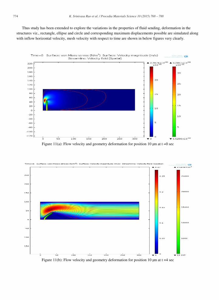
Thus study has been extended to explore the variations in the properties of fluid sending, deformation in the structures viz., rectangle, ellipse and circle and corresponding maximum displacements possible are simulated along with inflow horizontal velocity, mesh velocity with respect to time are shown in below figures very clearly.

Figure 11(a): Flow velocity and geometry deformation for position 10 m at t =0 sec

Figure 11(b): Flow velocity and geometry deformation for position 10 m at t =4 sec

775 K. Srinivasa Rao et al. / Procedia Materials Science 10 ( 2015 ) 768 – 788

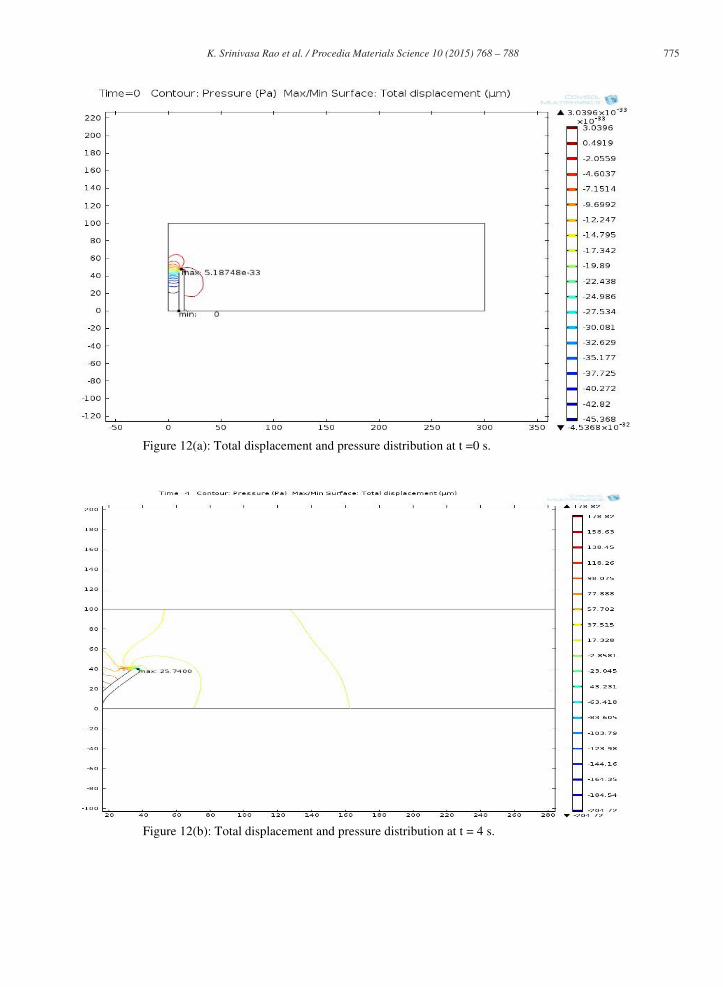
Figure 12(a): Total displacement and pressure distribution at t =0 s.

Figure 12(b): Total displacement and pressure distribution at t = 4 s.

776 K. Srinivasa Rao et al. / Procedia Materials Science 10 ( 2015 ) 768 – 788

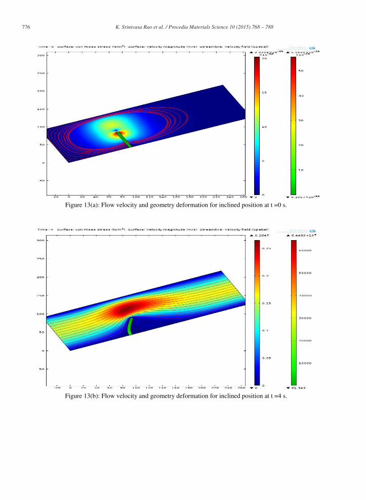
Figure 13(a): Flow velocity and geometry deformation for inclined position at t =0 s.

Figure 13(b): Flow velocity and geometry deformation for inclined position at t =4 s.

777 K. Srinivasa Rao et al. / Procedia Materials Science 10 ( 2015 ) 768 – 788

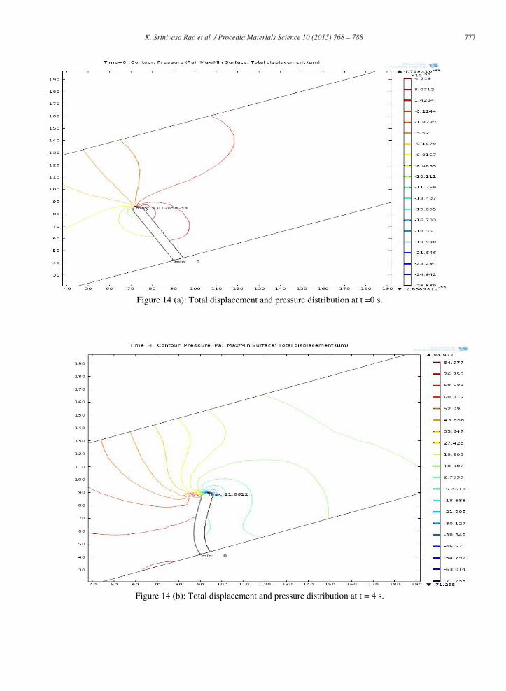
Figure 14 (a): Total displacement and pressure distribution at t =0 s.

Figure 14 (b): Total displacement and pressure distribution at t = 4 s.

778 K. Srinivasa Rao et al. / Procedia Materials Science 10 ( 2015 ) 768 – 788

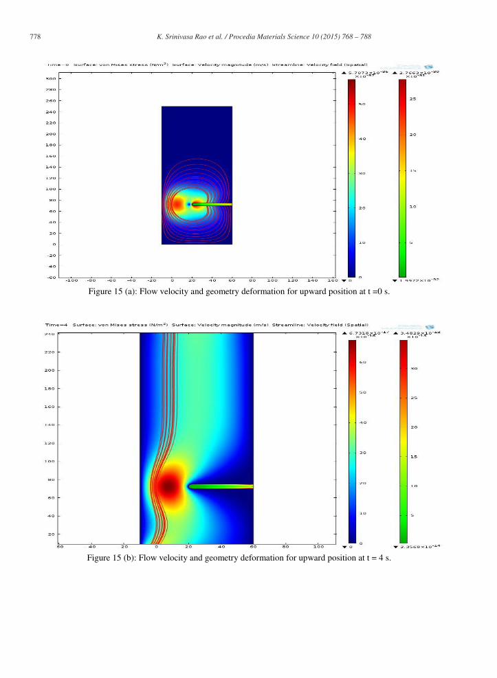
Figure 15 (a): Flow velocity and geometry deformation for upward position at t =0 s.

Figure 15 (b): Flow velocity and geometry deformation for upward position at t = 4 s.

779 K. Srinivasa Rao et al. / Procedia Materials Science 10 ( 2015 ) 768 – 788

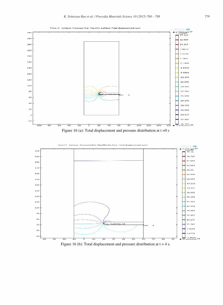
Figure 16 (a): Total displacement and pressure distribution at t =0 s

Figure 16 (b): Total displacement and pressure distribution at t = 4 s.

780 K. Srinivasa Rao et al. / Procedia Materials Science 10 ( 2015 ) 768 – 788

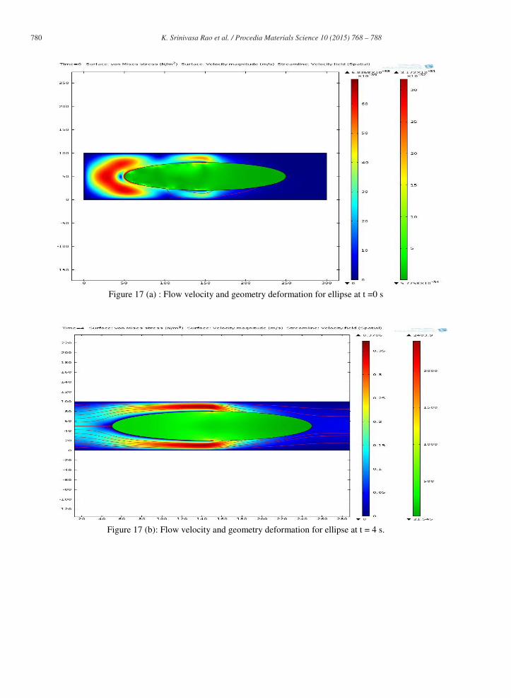
Figure 17 (a) : Flow velocity and geometry deformation for ellipse at t =0 s

Figure 17 (b): Flow velocity and geometry deformation for ellipse at t = 4 s.

781 K. Srinivasa Rao et al. / Procedia Materials Science 10 ( 2015 ) 768 – 788

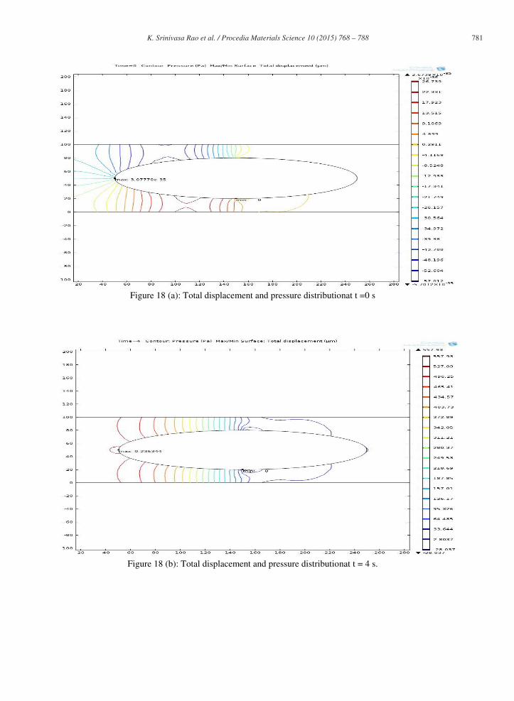
Figure 18 (a): Total displacement and pressure distributionat t =0 s

Figure 18 (b): Total displacement and pressure distributionat t = 4 s.

782 K. Srinivasa Rao et al. / Procedia Materials Science 10 ( 2015 ) 768 – 788

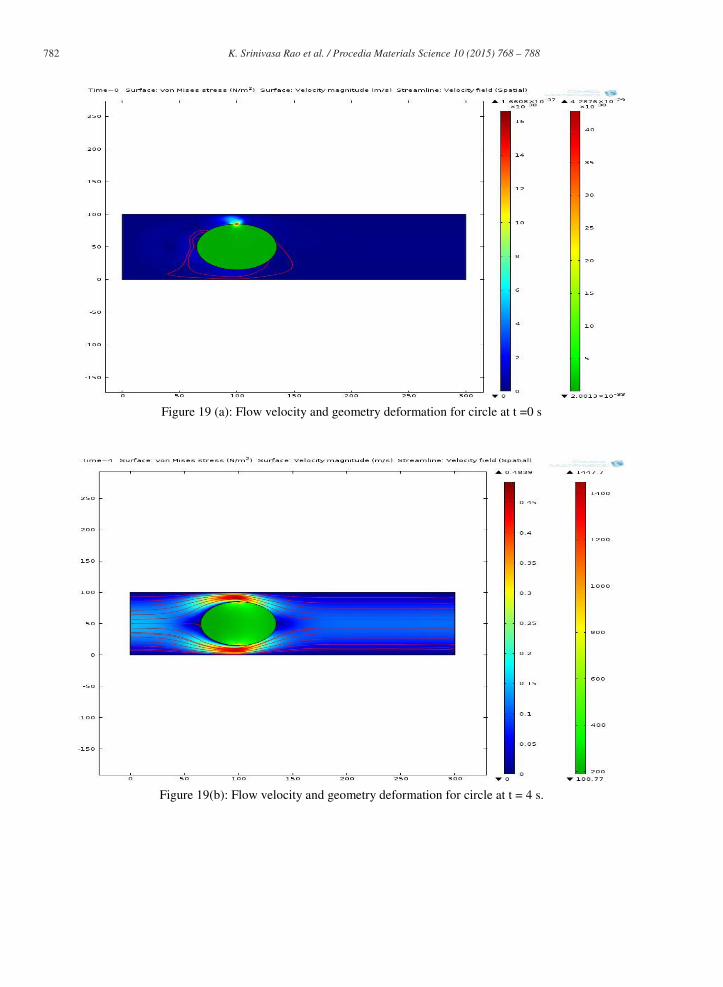
Figure 19 (a): Flow velocity and geometry deformation for circle at t =0 s

Figure 19(b): Flow velocity and geometry deformation for circle at t = 4 s.

783 K. Srinivasa Rao et al. / Procedia Materials Science 10 ( 2015 ) 768 – 788

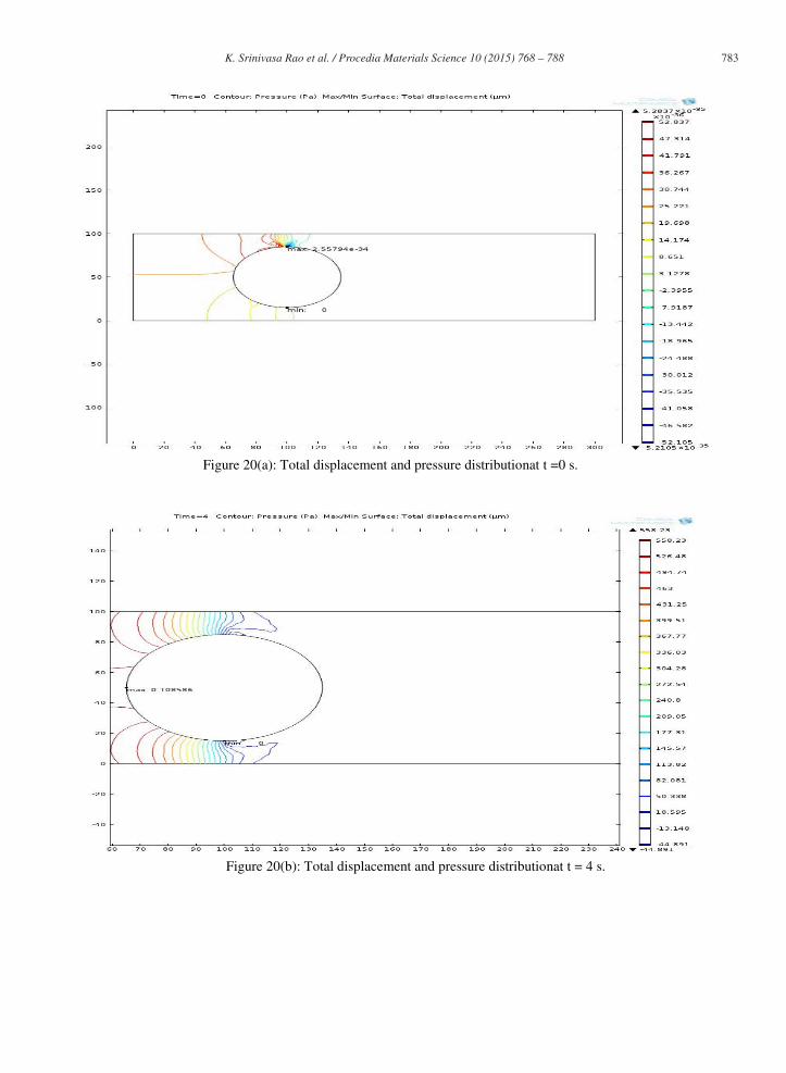
Figure 20(a): Total displacement and pressure distributionat t =0 s.

Figure 20(b): Total displacement and pressure distributionat t = 4 s.

784 K. Srinivasa Rao et al. / Procedia Materials Science 10 ( 2015 ) 768 – 788

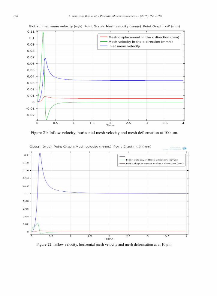
Figure 21: Inflow velocity, horizontal mesh velocity and mesh deformation at 100 m.

Figure 22: Inflow velocity, horizontal mesh velocity and mesh deformation at at 10 m.

785 K. Srinivasa Rao et al. / Procedia Materials Science 10 ( 2015 ) 768 – 788

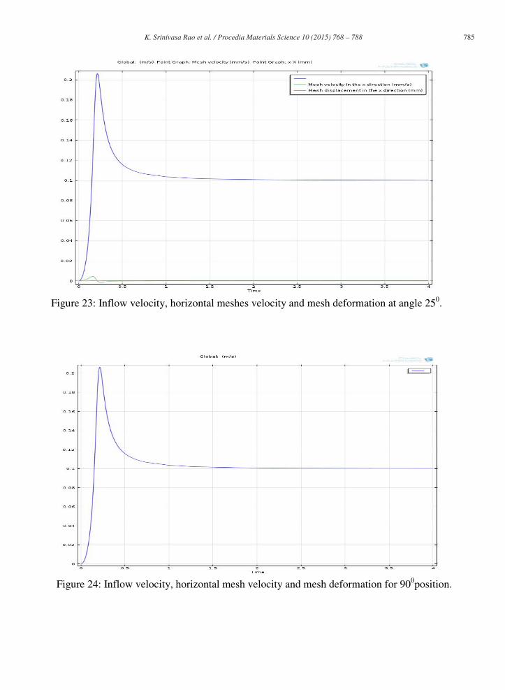
Figure 23: Inflow velocity, horizontal meshes velocity and mesh deformation at angle 250.

Figure 24: Inflow velocity, horizontal mesh velocity and mesh deformation for 900position.

786 K. Srinivasa Rao et al. / Procedia Materials Science 10 ( 2015 ) 768 – 788

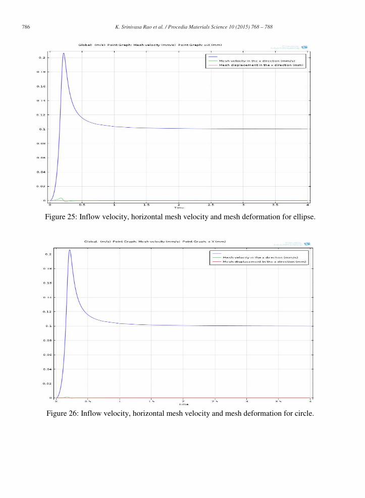
Figure 25: Inflow velocity, horizontal mesh velocity and mesh deformation for ellipse.

Figure 26: Inflow velocity, horizontal mesh velocity and mesh deformation for circle.

787 K. Srinivasa Rao et al. / Procedia Materials Science 10 ( 2015 ) 768 – 788

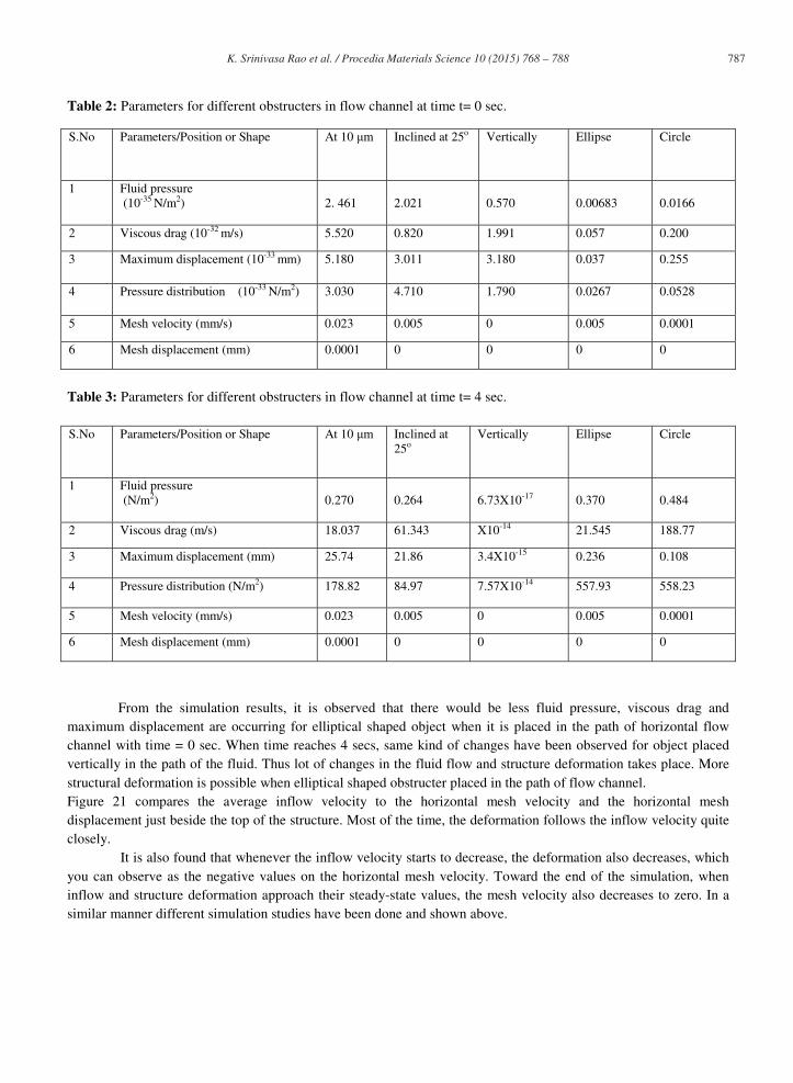
Table 2: Parameters for different obstructers in flow channel at time t= 0 sec. S.No Parameters/Position or Shape At 10 m Inclined at 25o Vertically Ellipse Circle

1 Fluid pressure (10-35 N/m2)

2. 461

2.021

0.570

0.00683

0.0166

2 Viscous drag (10-32 m/s) 5.520 0.820 1.991 0.057 0.200

3 Maximum displacement (10-33 mm) 5.180 3.011 3.180 0.037 0.255

4 Pressure distribution (10-33 N/m2) 3.030 4.710 1.790 0.0267 0.0528

5 Mesh velocity (mm/s) 0.023 0.005 0 0.005 0.0001

6 Mesh displacement (mm) 0.0001 0 0 0 0

Table 3: Parameters for different obstructers in flow channel at time t= 4 sec.

S.No Parameters/Position or Shape At 10 m Inclined at

25o Vertically Ellipse Circle

1 Fluid pressure (N/m2)

0.270

0.264

6.73X10-17

0.370

0.484

2 Viscous drag (m/s) 18.037 61.343 X10-14 21.545 188.77

3 Maximum displacement (mm) 25.74 21.86 3.4X10-15 0.236 0.108

4 Pressure distribution (N/m2) 178.82 84.97 7.57X10-14 557.93 558.23

5 Mesh velocity (mm/s) 0.023 0.005 0 0.005 0.0001

6 Mesh displacement (mm) 0.0001 0 0 0 0

From the simulation results, it is observed that there would be less fluid pressure, viscous drag and maximum displacement are occurring for elliptical shaped object when it is placed in the path of horizontal flow channel with time = 0 sec. When time reaches 4 secs, same kind of changes have been observed for object placed vertically in the path of the fluid. Thus lot of changes in the fluid flow and structure deformation takes place. More structural deformation is possible when elliptical shaped obstructer placed in the path of flow channel. Figure 21 compares the average inflow velocity to the horizontal mesh velocity and the horizontal mesh displacement just beside the top of the structure. Most of the time, the deformation follows the inflow velocity quite closely. It is also found that whenever the inflow velocity starts to decrease, the deformation also decreases, which you can observe as the negative values on the horizontal mesh velocity. Toward the end of the simulation, when inflow and structure deformation approach their steady-state values, the mesh velocity also decreases to zero. In a similar manner different simulation studies have been done and shown above.

788 K. Srinivasa Rao et al. / Procedia Materials Science 10 ( 2015 ) 768 – 788

6. Conclusions

MEMS based fluid flow channel is designed and its structural interaction was analysed using COMSOL Multiphysics Version 4.2 a. Simulation for the proposed model is done by changing the flow rates of the input mean velocity and also the shape of the obstacles placing in the path of the fluid to explore the variations in the properties of fluid sending, deformation in the structures viz., rectangle, ellipse and circle and corresponding maximum displacements with respect to time. From the analyses of results, the design of elliptical shaped obstructer was exhibiting predominant results in such a way that fluid pressure distribution, maximum displacement, viscous drag values are very less when compared with the other shapes of the obstructers. Thus we found that the flow channel is more deformed when ellipse structure is placed and it also confirms that obstructor occupying larger dimensional area in the flow channel would be in its steady state position. Finally, it would be useful for the situations containing fluid flow to illustrate the structure deformation with fluid flow and how to solve for the flow in a continuously deforming geometry using the arbitrary Lagrangian-Eulerian (ALE) technique. References

D.E Ingber., 2003, Cell structure and hierarchical systems biology,” J. Cell Sci., 116, 1157-73. M. Heil, 2004, An efficient solver for the fully coupled solution of large-displacement fluid-structure interaction problems. Computer Methods in Applied Mechanics and Engineering 193, 1–23. MEMS module (Model library), Comsol Multiphysics 3.5a. K.J. Bathe, H. Zhang. 2004, Finite element developments for general fluid flows with structural interactions". International Journal for Numerical Methods in Engineering 60, 213–232. J. Hron, S. Turek, 2006, A monolithic FEM/multigrid solver for ALE formulation of fluid-structure interaction with application in biomechanics.