Embed Size (px)
Citation preview
7/24/2019 DESIGN AND ANALYSIS OF ORIFICES
http://slidepdf.com/reader/full/design-and-analysis-of-orifices 1/46
i
DESIGN AND ANALYSIS OF ORIFICES FOR USE
IN NUCLEAR REACTOR COOLANT PUMPTEST LOOPS
by
Jeffrey Robert Stack
An Engineering Project Submitted to the Graduate
Faculty of Rensselaer Polytechnic Institute
in Partial Fulfillment of the
Requirements for the degree of
MASTER OF ENGINEERING IN MECHANICAL ENGINEERING
Approved:
_________________________________________Ernesto Gutierrez-Miravete, Adviser
Rensselaer Polytechnic Institute
Hartford, CT
December 2011

7/24/2019 DESIGN AND ANALYSIS OF ORIFICES
http://slidepdf.com/reader/full/design-and-analysis-of-orifices 2/46
ii
CONTENTS
LIST OF TABLES ............................................................................................................ iii
LIST OF FIGURES .......................................................................................................... iv
LIST OF SYMBOLS ......................................................................................................... v
ACKNOWLEDGMENT .................................................................................................. vi
ABSTRACT .................................................................................................................... vii
1. Introduction.................................................................................................................. 1
2. Theory & Methodology ............................................................................................... 5
3. Results and Discussion ................................................................................................ 7
3.1 Determination of Required Orifice Differential Pressures ................................. 7
3.2 Sizing of Orifice 1 .............................................................................................. 9
3.3 Sizing of Orifice 2 ............................................................................................ 12
3.4 Numerical Method for Calculation of Orifice Pressure Drop .......................... 14
3.5 Static Structural Analysis of Orifice ................................................................ 20
3.6 Modal Analysis of Orifices .............................................................................. 28
4. Conclusions................................................................................................................ 31
5.
References .................................................................................................................. 33
Appendix A: Orifice Mode Shapes .................................................................................. 34

7/24/2019 DESIGN AND ANALYSIS OF ORIFICES
http://slidepdf.com/reader/full/design-and-analysis-of-orifices 3/46
iii
LIST OF TABLES
Table 1: COMSOL Mesh Comparison ............................................................................ 16
Table 2: ANSYS Mesh Comparison................................................................................ 23
Table 3: Orifice Natural Frequencies .............................................................................. 29

7/24/2019 DESIGN AND ANALYSIS OF ORIFICES
http://slidepdf.com/reader/full/design-and-analysis-of-orifices 4/46
iv
LIST OF FIGURES
Figure 1: Examples of Cavitation Damage [3] .................................................................. 2
Figure 2: Pump Impeller & Diffuser [5] ............................................................................ 4
Figure 3: Typical Pump Curve .......................................................................................... 7
Figure 4: Pump Curve with Two Operating Points ........................................................... 8
Figure 5: Diagram of Thick-Edged Orifice [6] ................................................................ 10
Figure 6: Geometry of COMSOL Model ........................................................................ 15
Figure 7: Auto-Meshing of COMSOL Model ................................................................. 15
Figure 8: Velocity Streamlines through COMSOL Model .............................................. 17
Figure 9: Magnified View of Recirculation Zone ........................................................... 17
Figure 10: Pressure Contour Plot ..................................................................................... 18
Figure 11: Pressure Along Axis of Symmetry ................................................................. 19
Figure 12: ANSYS Workbench Geometry ...................................................................... 21
Figure 13: ANSYS Workbench Model Meshing............................................................. 22
Figure 14: COMSOL Pressure Plot Along Orifice Face ................................................. 24
Figure 15: Setup of ANSYS Model ................................................................................. 25
Figure 16: Deformation of ANSYS Model ..................................................................... 26
Figure 17: Stress Intensity of ANSYS Model ................................................................. 26
7/24/2019 DESIGN AND ANALYSIS OF ORIFICES
http://slidepdf.com/reader/full/design-and-analysis-of-orifices 5/46
v
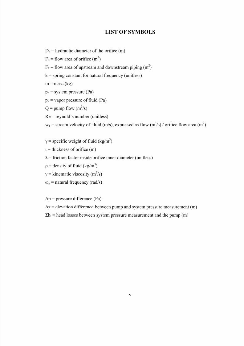
LIST OF SYMBOLS
Dh = hydraulic diameter of the orifice (m)
F0 = flow area of orifice (m
2
)F1 = flow area of upstream and downstream piping (m
2)
k = spring constant for natural frequency (unitless)
m = mass (kg)
po = system pressure (Pa)
pv = vapor pressure of fluid (Pa)
Q = pump flow (m3/s)
Re = reynold’s number (unitless)
w1 = stream velocity of fluid (m/s), expressed as flow (m3/s) / orifice flow area (m
2)
γ = specific weight of fluid (kg/m3)
ι = thickness of orifice (m)
λ = friction factor inside orifice inner diameter (unitless)
ρ = density of fluid (kg/m3)
ν = kinematic viscosity (m2/s)
ωn = natural frequency (rad/s)
Δ p = pressure difference (Pa)
Δz = elevation difference between pump and system pressure measurement (m)
Σhl = head losses between system pressure measurement and the pump (m)

7/24/2019 DESIGN AND ANALYSIS OF ORIFICES
http://slidepdf.com/reader/full/design-and-analysis-of-orifices 6/46
vi
ACKNOWLEDGMENT
I would like to express my gratitude to Dr. Gutierrez-Miravete for support throughout
this project and through my degree program. I would also like to thank all of my family
and friends that supported me through my time spent at Rensselaer Polytechnic Institute.Finally, I would like to express my gratitude to my professional associates that have
provided support for through the program.
7/24/2019 DESIGN AND ANALYSIS OF ORIFICES
http://slidepdf.com/reader/full/design-and-analysis-of-orifices 7/46
vii
ABSTRACT
This report describes results from a project aimed at sizing orifices installed in a typical
test loop for Reactor Coolant Pumps (RCPs) for use in Pressurized Water Reactor
(PWR) power plants. These orifices are used to simulate the hydraulic resistance of theReactor Coolant System (RCS) in a PWR power plant, which includes the resistance of
the reactor core and steam generators. PWR power plants use centrifugal, single-stage
RCPs to cool the reactor and transfer heat to the steam generators. These RCPs are
typically required to be full-scale performance tested prior to shipment to the power
plant site to ensure they meet all design requirements. To perform this testing, the RCPs
are temporarily installed in test loops where water is circulated through the loop at
different operating conditions. In this project, both analytical and numerical methods are
used to size the orifices such that they accurately simulate the system resistance of the
RCS for use in the test loop. Using results from the sizing calculations, a static
structural analysis is performed to confirm that the orifice design can withstand the
hydraulic forces seen during testing. Finally, a modal analysis is performed to determine
the orifice natural frequencies. These natural frequencies are compared with RCP
hydraulic pressure pulsation frequencies to ensure that they do not overlap and induce a
harmonic excitation of the orifices.
7/24/2019 DESIGN AND ANALYSIS OF ORIFICES
http://slidepdf.com/reader/full/design-and-analysis-of-orifices 8/46
1
1. Introduction
Reactor Coolant Pumps (RCPs) are the main pumps in a Pressurized Water Reactor’s
(PWRs) Reactor Coolant System (RCS), which provide flow of high temperature and
high pressure sub-cooled water to the nuclear reactor. This flow cools the reactor andtransfers the thermal energy from the reactor to the steam generator, which produces
steam to turn turbines, thereby producing power for public consumption. RCPs used in
PWRs are typically vertical, single-stage centrifugal pumps as RCPs require large
volume flows, minimal pressure pulsations through the RCS and easy access for
maintenance. A typical nuclear plant will have between two and four RCPs, each of
which circulates on the order of 100,000gpm of water through the RCS [1]. These
pumps are generally required to be full scale performance tested prior to shipment to the
power plant site. This performance testing proves the mechanical and hydraulic design
and functionality of each RCP prior to shipment in order to minimize risk. To test these
very large pumps, they must be temporarily installed into a test loop at the
manufacturing/testing facility where each pump is operated at various temperatures,
pressures and flows to match expected plant conditions. To ensure proper performance
when installed into the RCS, many aspects of each pump design must be tested such as
hydraulic performance, vibrations, and efficiency, Net Positive Suction Head Required
(NPSHR), hydraulic pressure pulsations and expected transient conditions among others.
As a result of the required testing, the conditions that the RCPs and the test loop are
subjected to are relatively extreme. According to Reference [2], normal operation
temperatures are between 530°F (276.7°C) and 590°F (310°C), pressures are typically
2250 psi (15.51MPa) and normal flows are roughly 100,000 gpm [1]. All test loop
components must be designed to withstand all potential testing conditions. This includes
the test loop piping, any penetrations into the test loop piping, flow meters, orifices and
valves.
One aspect of the testing program that subjects the pump and test loop to particularly
harsh conditions is NPSHR testing. NPSHR is the minimum NPSH required by the
pump to avoid damage to the pump hydraulics due to cavitation. Cavitation can quickly

7/24/2019 DESIGN AND ANALYSIS OF ORIFICES
http://slidepdf.com/reader/full/design-and-analysis-of-orifices 9/46
2
cause irreparable damage to a set of pump hydraulics due to the violent shock waves
generated as the cavitation bubbles collapse. Figure 1 [3] shows examples of damage
caused by cavitation.
Figure 1: Examples of Cavitation Damage [3]
As a result of the very low system pressures in the test loop during NPSHR testing,
cavitation becomes a concern for all parts of the test loop, not just the pump itself. Of
particular concern is the main flow restricting components of the test loop that provide
the resistance to the pump to simulate the resistances of the reactor internals and steam
generators. This is because these components reduce the cross section flow area,
resulting in significantly higher flow rates. Since NPSH available is reduced as flow is
increased, the high flow rates through these components make them particularly
vulnerable to cavitation and its damaging effects.
Cavitation damage to test loop components can be detrimental to a testing program.
Damage could have effect on their intended resistance, measuring capability or worse, broken components flowing through the test loop could cause irreparable damage to the
pump hydraulics.
One way to try to prevent cavitation at the main flow restricting components of the test
loop is to provide the required pressure drop in stages. For instance, two large inner
7/24/2019 DESIGN AND ANALYSIS OF ORIFICES
http://slidepdf.com/reader/full/design-and-analysis-of-orifices 10/46
3
diameter orifices installed in series would be preferable to one small inner diameter
orifice. This is because the velocity of the fluid flowing through the orifice increases as
it passes through it. Increasing the velocity is undesirable as Bernoulli’s Principle tells
us that as velocity increases, pressure decreases and as pressure decreases so does
available NPSH according to the equation below.
∆ ∑
[4]
Where:
po = system pressure (Pa)
γ = specific weight of fluid (kg/m3)
Δz = elevation difference between pump and system pressure measurement (m)
Σhl = head losses between system pressure measurement and the pump (m)
pv = vapor pressure of fluid (Pa)
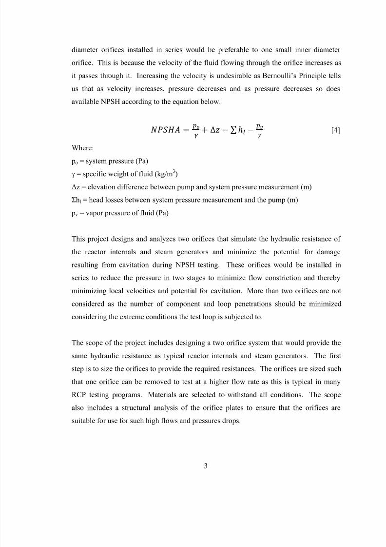
This project designs and analyzes two orifices that simulate the hydraulic resistance of
the reactor internals and steam generators and minimize the potential for damage
resulting from cavitation during NPSH testing. These orifices would be installed in
series to reduce the pressure in two stages to minimize flow constriction and thereby
minimizing local velocities and potential for cavitation. More than two orifices are not
considered as the number of component and loop penetrations should be minimized
considering the extreme conditions the test loop is subjected to.
The scope of the project includes designing a two orifice system that would provide the
same hydraulic resistance as typical reactor internals and steam generators. The first
step is to size the orifices to provide the required resistances. The orifices are sized such
that one orifice can be removed to test at a higher flow rate as this is typical in manyRCP testing programs. Materials are selected to withstand all conditions. The scope
also includes a structural analysis of the orifice plates to ensure that the orifices are
suitable for use for such high flows and pressures drops.
7/24/2019 DESIGN AND ANALYSIS OF ORIFICES
http://slidepdf.com/reader/full/design-and-analysis-of-orifices 11/46
4
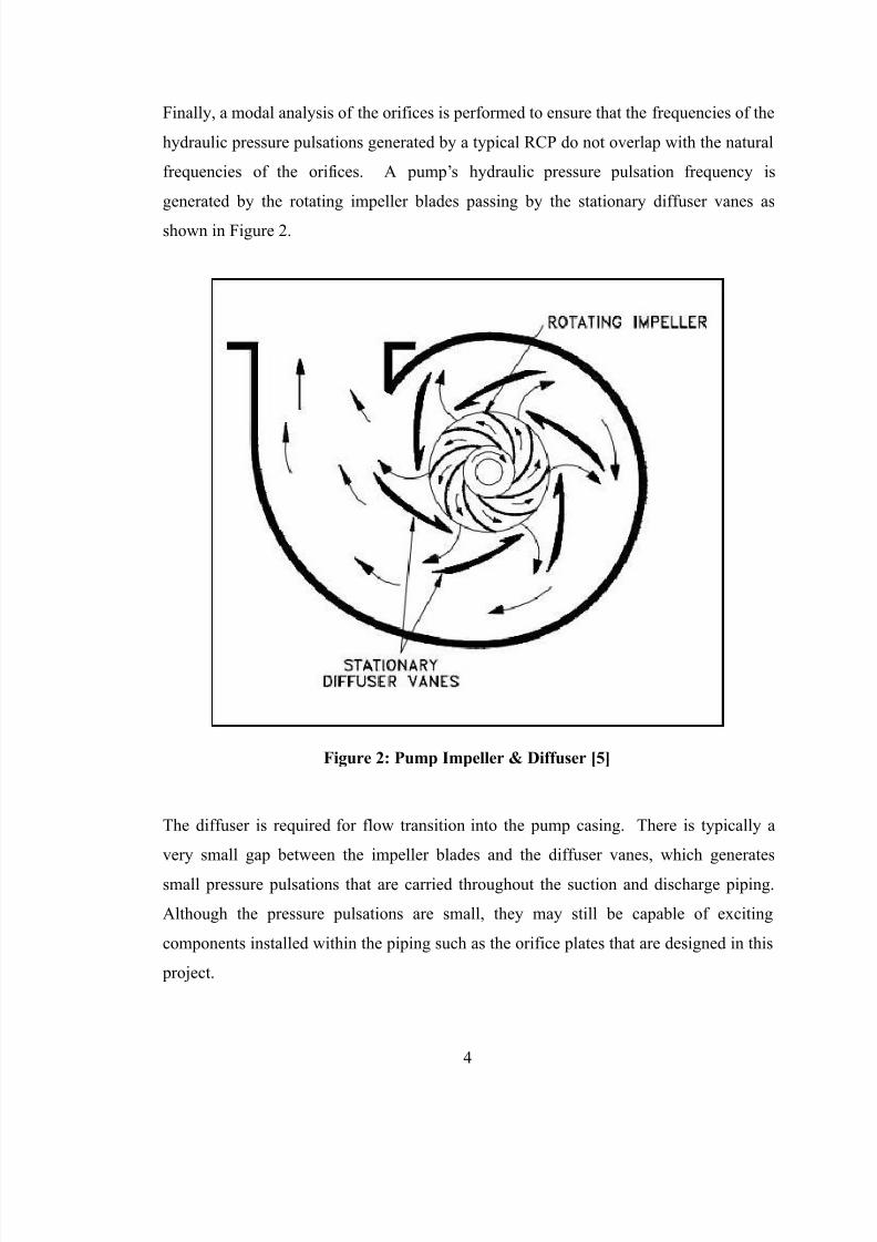
Finally, a modal analysis of the orifices is performed to ensure that the frequencies of the
hydraulic pressure pulsations generated by a typical RCP do not overlap with the natural
frequencies of the orifices. A pump’s hydraulic pressure pulsation frequency is
generated by the rotating impeller blades passing by the stationary diffuser vanes as
shown in Figure 2.
Figure 2: Pump Impeller & Diffuser [5]
The diffuser is required for flow transition into the pump casing. There is typically a
very small gap between the impeller blades and the diffuser vanes, which generates
small pressure pulsations that are carried throughout the suction and discharge piping.
Although the pressure pulsations are small, they may still be capable of exciting
components installed within the piping such as the orifice plates that are designed in this
project.

7/24/2019 DESIGN AND ANALYSIS OF ORIFICES
http://slidepdf.com/reader/full/design-and-analysis-of-orifices 12/46
5
2. Theory & Methodology
The first step of the problem is to size and design the orifices to provide the required
resistances. The dual-orifice system is designed such that both orifices installed in series
provide the required resistance to achieve the low flow (rated head and flow) point.Further, they are sized so that when one orifice (Orifice 2) is removed, the remaining
orifice (Orifice 1) provides the required resistance to achieve the high flow point. For
this high flow point, a slope of the pump curve and a high flow rate is assumed. Then,
using this information and the rated head and flow of the RCP, the head and flow of the
high flow point is determined and the required resistance of Orifice 1 is known.
Once the required resistance of Orifice 1 is known for the high flow condition, it is sized
using a correlation from Reference [6]. This results in an inner diameter for Orifice 1.
To determine the inner diameter for Orifice 2 (installed to achieve low flow point), the
resistance of Orifice 1 is recalculated for the low flow condition and subtracted from the
total required resistance (defined by the rated pump head). Then, the same correlation
that was used to size Orifice 1 is used to size Orifice 2. Checks of Reynolds Numbers
and ι/Dh are performed to ensure that use of the correlation is appropriate.
Once the orifices have been sized using analytical methods, the orifice and flow
condition that provide the highest pressure drop is solved numerically for comparison
with the analytical pressure drop. This also represents the worst case condition for
stresses within the orifice and may be used for input into structural analyses, if the
numerical methods prove to be more conservative. As a result, numerical flow analysis
of only one orifice is necessary.
To solve for the pressure drop and the hydraulic forces numerically, the finite element
software COMSOL Multiphysics is used. The same geometry and same inputs are used
as in the analytical method. The auto-meshing feature of the software is used to generate
the number of elements, their size and their shape. Multiple cases are run with different
mesh sizes to ensure that the mesh is small enough to produce accurate results. In
7/24/2019 DESIGN AND ANALYSIS OF ORIFICES
http://slidepdf.com/reader/full/design-and-analysis-of-orifices 13/46
6
addition, a minimum distance between the two orifices can be determined from this
model.
Finally, a structural analysis is performed to ensure that the orifice remains structurally
sound throughout all expected testing conditions. This is especially important
considering that any damage to the orifices could result in damage to the pump
hydraulics, which is the saleable equipment. 3-D models of the orifice designs are then
generated using the finite element software ANSYS Workbench. These models are then
analyzed for the worst-case scenario, which is defined as the orifice and flow condition
that provide the greatest pressure drop. Resulting stresses are compared to the yield
strength of the selected material to confirm the appropriateness of the assumed material
and orifice thickness.
An additional modal analysis of the orifices is performed to ensure that the frequencies
of the hydraulic pressure pulsations generated by a typical pump do not overlap with the
natural frequencies of the orifices. This modal analysis is performed on both orifices as
a conservative condition does not exist. Natural frequencies of the both orifices are
compared with hydraulic pressure pulsations of a typical RCP.
7/24/2019 DESIGN AND ANALYSIS OF ORIFICES
http://slidepdf.com/reader/full/design-and-analysis-of-orifices 14/46
7
3. Results and Discussion
3.1 Determination of Required Orifice Differential Pressures
The first step in defining the geometry of the two orifices that will be used to simulate
the hydraulic resistance of the main Reactor Coolant System (RCS) is to determine what
resistances will be required of them to achieve the desired test flow rates and
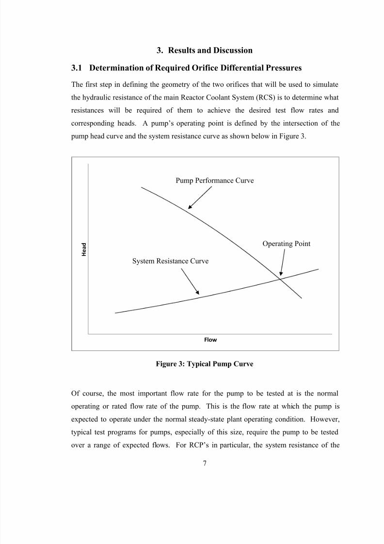
corresponding heads. A pump’s operating point is defined by the intersection of the
pump head curve and the system resistance curve as shown below in Figure 3.
Figure 3: Typical Pump Curve
Of course, the most important flow rate for the pump to be tested at is the normal
operating or rated flow rate of the pump. This is the flow rate at which the pump is
expected to operate under the normal steady-state plant operating condition. However,
typical test programs for pumps, especially of this size, require the pump to be tested
over a range of expected flows. For RCP’s in particular, the system resistance of the
H e a d
Flow
System Resistance Curve
Pump Performance Curve
Operating Point
7/24/2019 DESIGN AND ANALYSIS OF ORIFICES
http://slidepdf.com/reader/full/design-and-analysis-of-orifices 15/46
8
RCS can be much lower than the normal operating system resistance if only one pump is
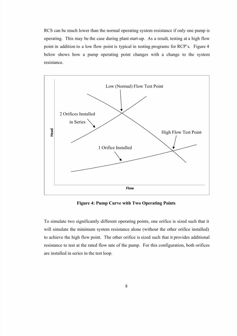
operating. This may be the case during plant start-up. As a result, testing at a high flow
point in addition to a low flow point is typical in testing programs for RCP’s. Figure 4
below shows how a pump operating point changes with a change to the system
resistance.
Figure 4: Pump Curve with Two Operating Points
To simulate two significantly different operating points, one orifice is sized such that it
will simulate the minimum system resistance alone (without the other orifice installed)
to achieve the high flow point. The other orifice is sized such that it provides additional
resistance to test at the rated flow rate of the pump. For this configuration, both orifices
are installed in series in the test loop.
H e a d
Flow
Low (Normal) Flow Test Point
High Flow Test Point
2 Orifices Installed
in Series
1 Orifice Installed
7/24/2019 DESIGN AND ANALYSIS OF ORIFICES
http://slidepdf.com/reader/full/design-and-analysis-of-orifices 16/46
9
The first step in sizing the orifices is to define the head and flow of the two test points.
The head is necessary as the required differential pressure (DP) across the orifice is
defined by the head of the pump. Flow is the test parameter that is typically required by
the test program. To define the two test points, the rated head and flow of Doosan’s
APR1400 Class Reactor Coolant Pump are chosen [7]. This pump was chosen as the
rated head and flow are relatively large as they will be used in a 1400MW power plant.
The large head and flow of this pump will provide generally conservative conditions at
the orifice plate.
The rated head of the Doosan APR1400 Class RCP is 114.3m and the rated flow is
7.672m3/s [7]. This will be the first of the two test points and will be referred to as the
rated test point. Both orifices installed in series will provide the resistance so that the
pump operates at this point. To determine the high flow test point, the slope of the pump
curve and the required test flow must be assumed as this is not information that is
publically available. Considering, it is assumed that the pump curve is linear, a typical
slope for the pump curve is negative 20m/(m3/s) and a typical high flow rate is 125% of
rated flow. The flow rate of the high flow test point is therefore 9.590m3/s.
Using this flow rate and the assumed slope of the pump curve, a high flow test point
head is determined to be 66.35m. The heads of the two test points, 114.3m and 66.35m,
are now be converted to pressures of 1143.0kPa and 663.5kPa, for use as necessary.
These are the DP’s required by the orifices to achieve the two test points. Normally,
other test loop piping losses would be considered, but for the purposes of this report,
these additional piping losses are considered negligible. This method also provides
conservative input to structural analyses.
3.2
Sizing of Orifice 1
Sizing of the first orifice which will be installed to achieve both test points will be based
on the requirement to provide a DP of 663.5kPa. From this point forward, it will be
designated as Orifice 1. To minimize constriction of the flow, a sharp edged orifice will
7/24/2019 DESIGN AND ANALYSIS OF ORIFICES
http://slidepdf.com/reader/full/design-and-analysis-of-orifices 17/46
10
be used as opposed to an orifice with a beveled or rounded leading edge. Further, there
are many good correlations to choose from for predicting the resistance of sharp edged
orifices. Erosion of the sharp edge over time should not be a concern as coolant water
that is pumped by RCP’s is extremely well controlled with no dissolved gases or
suspended solids and run time for testing is relatively low.
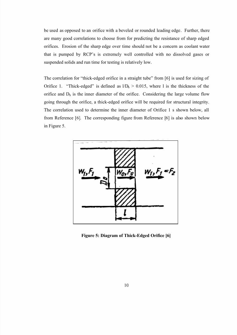
The correlation for “thick-edged orifice in a straight tube” from [6] is used for sizing of
Orifice 1. “Thick-edged” is defined as l/Dh > 0.015, where l is the thickness of the
orifice and Dh is the inner diameter of the orifice. Considering the large volume flow
going through the orifice, a thick-edged orifice will be required for structural integrity.
The correlation used to determine the inner diameter of Orifice 1 s shown below, all
from Reference [6]. The corresponding figure from Reference [6] is also shown below
in Figure 5.
Figure 5: Diagram of Thick-Edged Orifice [6]
7/24/2019 DESIGN AND ANALYSIS OF ORIFICES
http://slidepdf.com/reader/full/design-and-analysis-of-orifices 18/46
11
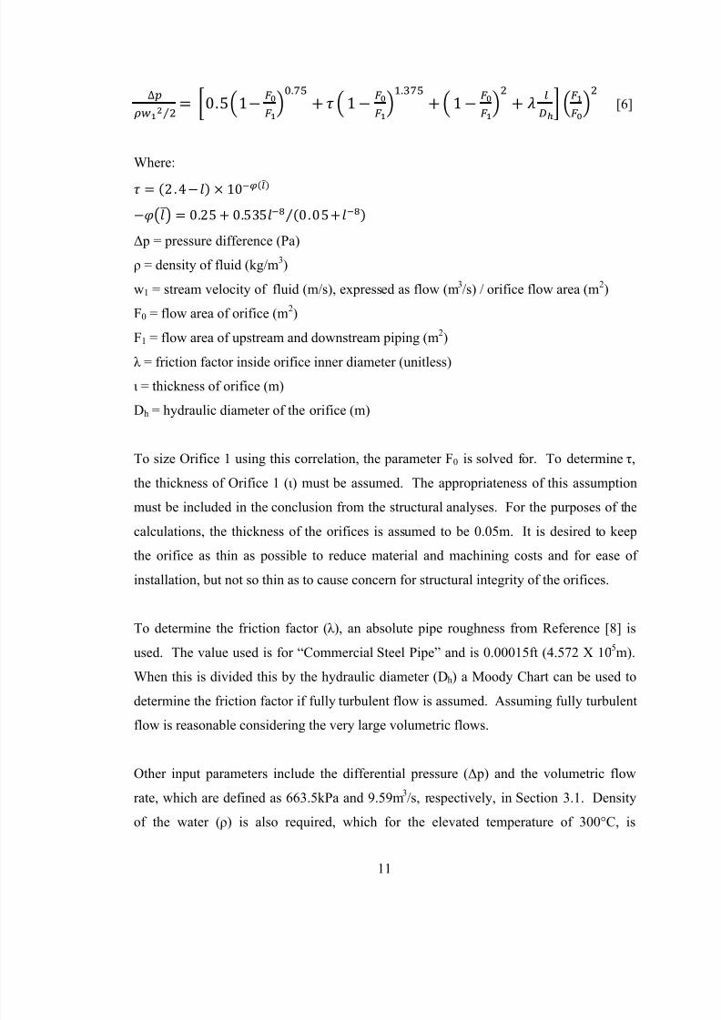
∆ ⁄ 0.51
. 1
. 1
[6]
Where:
2 . 4 10 0.25 0.535 0.05⁄
Δ p = pressure difference (Pa)
ρ = density of fluid (kg/m3)
w1 = stream velocity of fluid (m/s), expressed as flow (m3/s) / orifice flow area (m
2)
F0 = flow area of orifice (m2)
F1 = flow area of upstream and downstream piping (m2)
λ = friction factor inside orifice inner diameter (unitless)
ι = thickness of orifice (m)
Dh = hydraulic diameter of the orifice (m)
To size Orifice 1 using this correlation, the parameter F0 is solved for. To determine τ,
the thickness of Orifice 1 (ι) must be assumed. The appropriateness of this assumption
must be included in the conclusion from the structural analyses. For the purposes of the
calculations, the thickness of the orifices is assumed to be 0.05m. It is desired to keepthe orifice as thin as possible to reduce material and machining costs and for ease of
installation, but not so thin as to cause concern for structural integrity of the orifices.
To determine the friction factor (λ ), an absolute pipe roughness from Reference [8] is
used. The value used is for “Commercial Steel Pipe” and is 0.00015ft (4.572 X 10⁻⁵
m).
When this is divided this by the hydraulic diameter (Dh) a Moody Chart can be used to
determine the friction factor if fully turbulent flow is assumed. Assuming fully turbulent
flow is reasonable considering the very large volumetric flows.
Other input parameters include the differential pressure (Δ p) and the volumetric flow
rate, which are defined as 663.5kPa and 9.59m3/s, respectively, in Section 3.1. Density
of the water (ρ) is also required, which for the elevated temperature of 300°C, is
7/24/2019 DESIGN AND ANALYSIS OF ORIFICES
http://slidepdf.com/reader/full/design-and-analysis-of-orifices 19/46
12
714kg/m3 from Reference [9]. Flow area of the upstream and downstream piping (F1) is
also an input parameter and is defined as 0.785m2 [10]. When all of these inputs are
used, F0 is determined to be 0.2347m2, which corresponds to an inside diameter of
0.547m for Orifice 1.
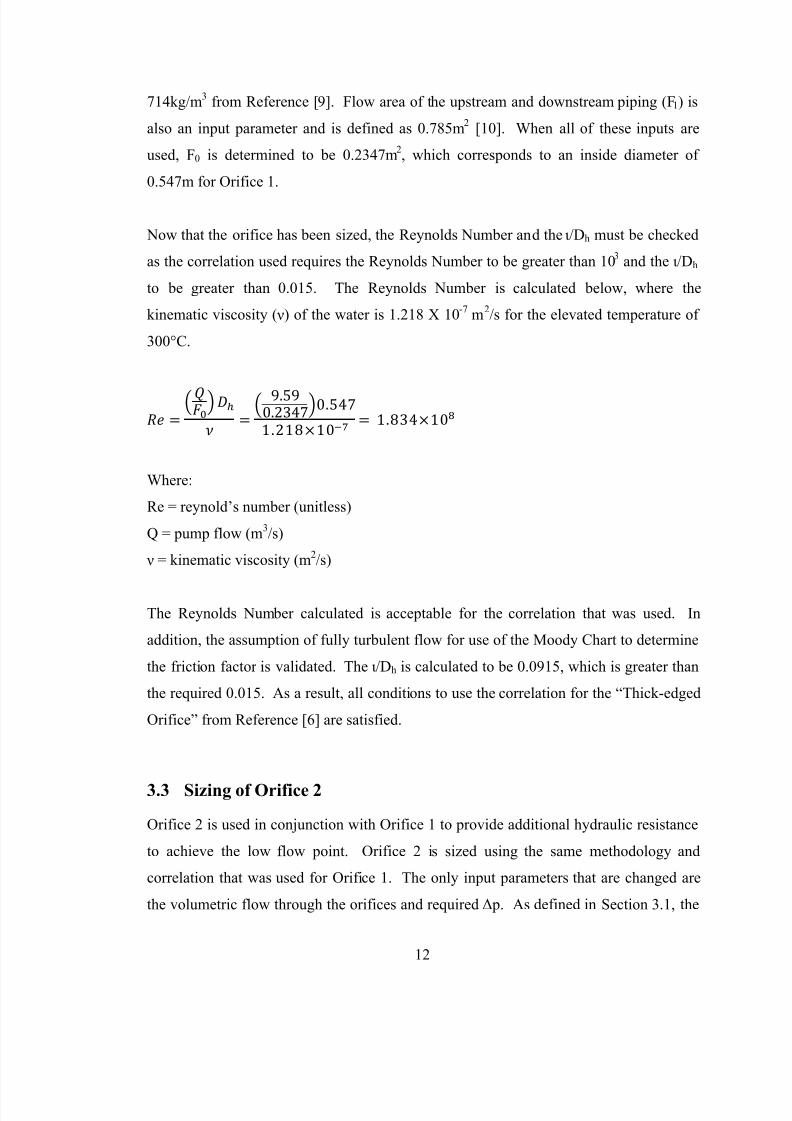
Now that the orifice has been sized, the Reynolds Number and the ι/Dh must be checked
as the correlation used requires the Reynolds Number to be greater than 103 and the ι/Dh
to be greater than 0.015. The Reynolds Number is calculated below, where the
kinematic viscosity ( ν) of the water is 1.218 X 10⁻⁷
m2/s for the elevated temperature of
300°C.
9.590.23470.547
1.21810 1.83410
Where:
Re = reynold’s number (unitless)
Q = pump flow (m3/s)
ν = kinematic viscosity (m2/s)
The Reynolds Number calculated is acceptable for the correlation that was used. In
addition, the assumption of fully turbulent flow for use of the Moody Chart to determine
the friction factor is validated. The ι/Dh is calculated to be 0.0915, which is greater than
the required 0.015. As a result, all conditions to use the correlation for the “Thick-edged
Orifice” from Reference [6] are satisfied.
3.3
Sizing of Orifice 2
Orifice 2 is used in conjunction with Orifice 1 to provide additional hydraulic resistance
to achieve the low flow point. Orifice 2 is sized using the same methodology and
correlation that was used for Orifice 1. The only input parameters that are changed are
the volumetric flow through the orifices and required Δ p. As defined in Section 3.1, the
7/24/2019 DESIGN AND ANALYSIS OF ORIFICES
http://slidepdf.com/reader/full/design-and-analysis-of-orifices 20/46
13
flow rate through the orifices is 7.672m3/s and the total required Δ p across the two
orifices is 1143.0kPa for the low flow point.
According to the correlation in Section 3.2, the Δ p of the orifice is dependent on the flow
rate. As a result, the Δ p for Orifice 1 must first be recalculated for the low flow point.
Using the flow area for Orifice 1 that was calculated in Section 3.2 and the low flow rate
of 7.672m3/s, the Δ p of Orifice 1 at the low flow point is calculated to be 266,565kPa.
With this, the required Δ p of Orifice 2 alone can finally be identified.
1,143,000 266,565 876,435
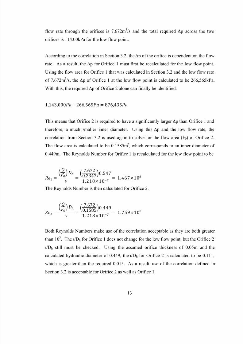
This means that Orifice 2 is required to have a significantly larger Δ p than Orifice 1 and
therefore, a much smaller inner diameter. Using this Δ p and the low flow rate, the
correlation from Section 3.2 is used again to solve for the flow area (F0) of Orifice 2.
The flow area is calculated to be 0.1585m2, which corresponds to an inner diameter of
0.449m. The Reynolds Number for Orifice 1 is recalculated for the low flow point to be
7.672
0.23470.547
1.21810 1.46710
The Reynolds Number is then calculated for Orifice 2.
7.6720.15850.4491.21810 1.75910
Both Reynolds Numbers make use of the correlation acceptable as they are both greater
than 10
3
. The ι/Dh for Orifice 1 does not change for the low flow point, but the Orifice 2ι/Dh still must be checked. Using the assumed orifice thickness of 0.05m and the
calculated hydraulic diameter of 0.449, the ι/Dh for Orifice 2 is calculated to be 0.111,
which is greater than the required 0.015. As a result, use of the correlation defined in
Section 3.2 is acceptable for Orifice 2 as well as Orifice 1.
7/24/2019 DESIGN AND ANALYSIS OF ORIFICES
http://slidepdf.com/reader/full/design-and-analysis-of-orifices 21/46
14
3.4 Numerical Method for Calculation of Orifice Pressure Drop
Generally, the analytical methods used in Sections 3.2 and 3.3 are considered to be very
accurate as the equation used has been developed from decades of empirical data.
However, for comparison, numerical methods for calculation of the Orifice DP are alsoexplored in this project. Use of one method over the other may depend on which method
provides the most conservative results.
For this project, the orifice and flow condition that provide the highest pressure drop are
analyzed numerically. This represents worst-case conditions for input into structural
analysis later in the project. The orifice and flow condition that provide the highest
pressure drop is Orifice 2, which is sized to provide a pressure drop of 876,435Pa to
achieve the low flow condition of 7.672m3/s. This orifice and surrounding piping are
modeled in the software COMSOL Multiphysics. Computational Fluid Dynamics
(CFD) is performed with this geometry and flow condition and the resulting pressure
drop is compared with the pressure drop that Orifice 2 was sized analytically to provide.
To build the model in COMSOL, the same inputs are used that are identified in Section
3.2. The density that is used is 714kg/m, the viscosity is 8.97X10⁻⁵
Pa(s). The diameter
of Orifice 2 is 0.449m. The lengths of the upstream and downstream piping were chosen
to capture all upstream and downstream effects, yet minimize total number of elements
so that computational time is minimized. The upstream pipe length was chosen to be
1.0m and the downstream pipe was selected to be 10m. The inlet velocity of the model
is specified to be 9.773m/s, which corresponds to the volumetric flow for the low flow
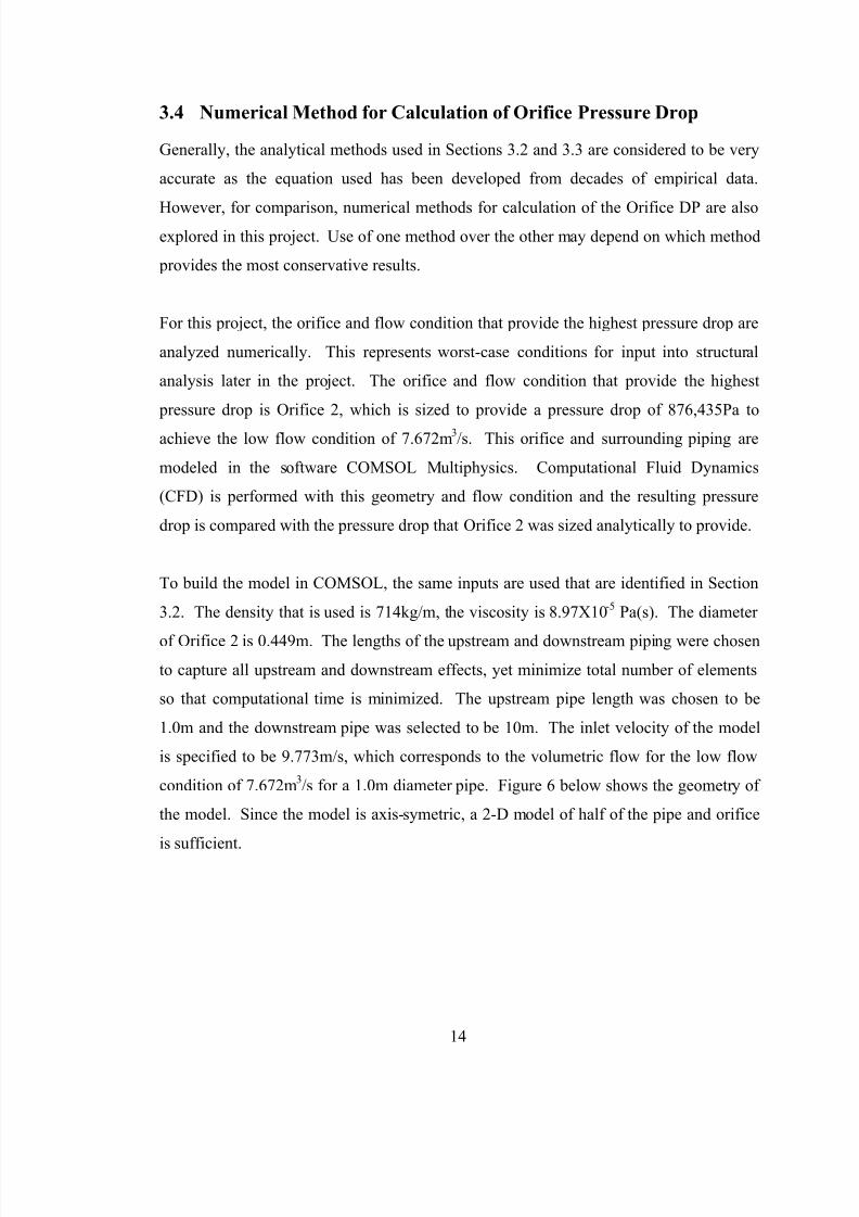
condition of 7.672m3/s for a 1.0m diameter pipe. Figure 6 below shows the geometry of
the model. Since the model is axis-symetric, a 2-D model of half of the pipe and orifice
is sufficient.
7/24/2019 DESIGN AND ANALYSIS OF ORIFICES
http://slidepdf.com/reader/full/design-and-analysis-of-orifices 22/46
15
FLOW Orifice
Axis of Symmetry
Figure 6: Geometry of COMSOL Model
Four different mesh sizes are used and their results are compared to justify that the
smallest mesh size is indeed small enough to be able to accurately compare with the
analytical results and potentially provide input values to the structural analysis of the
orifice. The auto-mesh function of COMSOL is used for meshing. This auto-meshing
creates appropriate mesh sizes and geometries at all locations within the model to
capture all fluid behavior, but to minimize computation time. Cases were run for auto-
mesh sizes of “Extremely Coarse”, “Extra Coarse”, “Coarser” and “Coarse”, listed
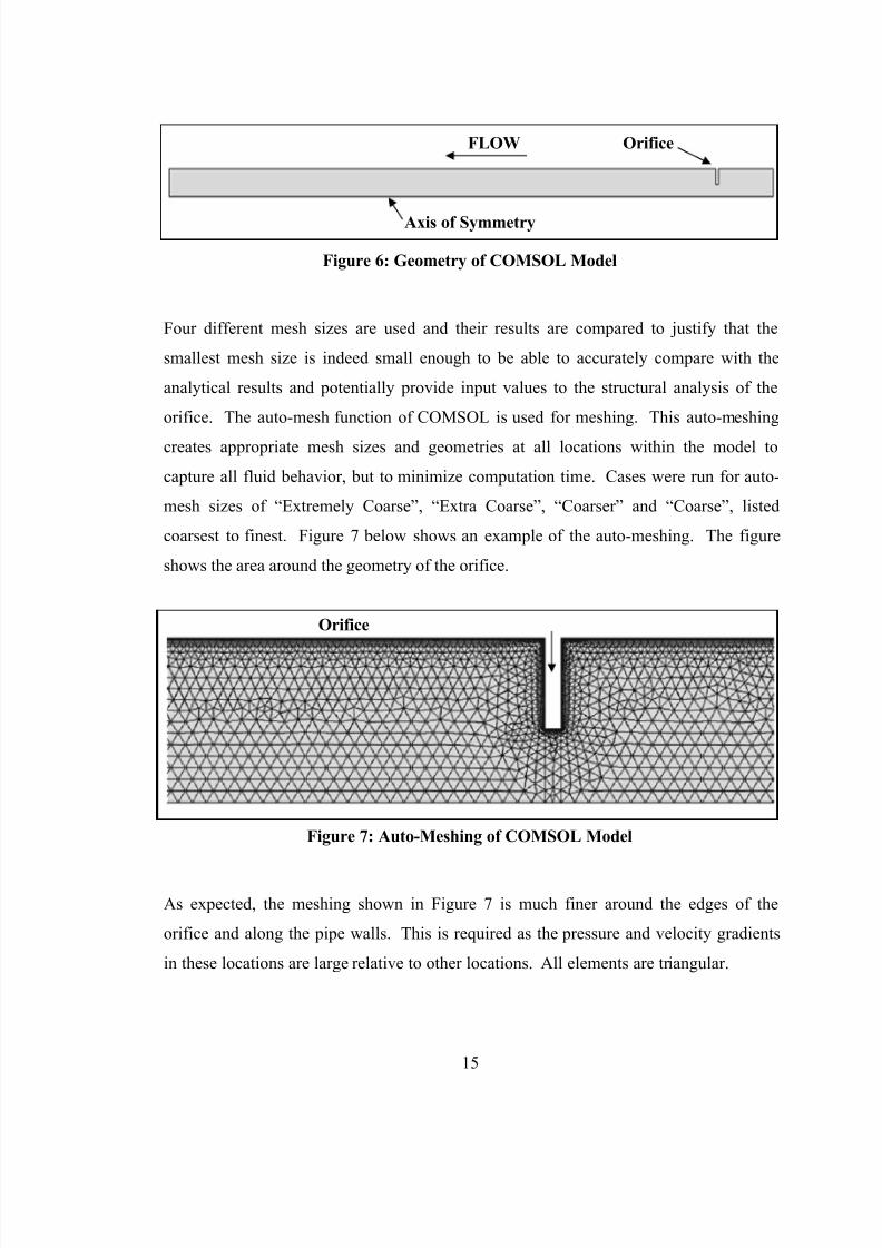
coarsest to finest. Figure 7 below shows an example of the auto-meshing. The figure
shows the area around the geometry of the orifice.
Orifice
Figure 7: Auto-Meshing of COMSOL Model
As expected, the meshing shown in Figure 7 is much finer around the edges of the
orifice and along the pipe walls. This is required as the pressure and velocity gradients
in these locations are large relative to other locations. All elements are triangular.

7/24/2019 DESIGN AND ANALYSIS OF ORIFICES
http://slidepdf.com/reader/full/design-and-analysis-of-orifices 23/46
16
The results of all four mesh sizes are compared and show diminishing returns as the
mesh size is decreased. The parameter that is compared between each case is the DP
from the inlet to the outlet of the entire model. The results from all four mesh sizes are
shown below in Table 1. The change between “Extremely Coarse” and “Extra Coarse”
is (1.4262-1.6495)/1.4262 = 15.66%. The change between “Extra Coarse” and
“Coarser” is 4.43% and the change between “Coarser” and “Coarse” is 0.18%. The
conclusion is that either the “Coarser” or “Coarse” auto-mesh setting is sufficient. The
results from the “Coarse” case are shown below.
Table 1: COMSOL Mesh Comparison
COMSOL Auto-
Mesh Size
Total Number of
Elements
Calculated Orifice
DP (MPa)Change (%)
Extremely Coarse 3,988 1.4262 N/A
Extra Coarse 6,916 1.6495 15.66
Coarser 13,443 1.5764 4.43
Coarse 21,099 1.5735 0.18
According to Reference [11], numerical methods generally perform three major steps to
solve a system. The first step is to perform integration of the governing equations over
the control volume. The resulting integral equations are then converted to a system of
algebraic equations. Finally, this system of algebraic equations is solved iteratively.
This is the general method used by COMSOL to solve the orifice flow system that is
described. Since this is a fluid flow system, the governing equations of the system
include conservation of mass, the first law of thermodynamics and Newton’s second law
[11]. When solving, certain assumptions may be made by the algorithm to simplify the
problem and facilitate its solution.
Figures 8 & 9 show the results of the COMSOL model. Figure 8 shows the velocity
streamlines of the entire system, while Figure 9 shows a magnified view of the velocity

7/24/2019 DESIGN AND ANALYSIS OF ORIFICES
http://slidepdf.com/reader/full/design-and-analysis-of-orifices 24/46
17
streamlines just downstream of the orifice. This area is referred to as the recirculation
zone.
FLOW Orifice
Figure 8: Velocity Streamlines through COMSOL Model
FLOW Orifice
Figure 9: Magnified View of Recirculation Zone
The velocity streamlines are typical for orifice flow. Because of the very high flow rate
and Reynold’s number, the flow is very uniform through upstream of the orifice and
downstream of the recirculation zone. The velocity boundary layer at the pipe wall is
very small. Figures 8 & 9 also show that the orifice only affects the upstream velocity
profile over a short distance, about 0.5m and that the downstream velocity profile (and
pressure) is not fully recovered until about 5.0m downstream of the orifice. This proves
that the upstream pipe length of 1.0m and the downstream pipe length of 10.0m are
sufficient. This is true for all mesh sizes.
Results of the COMSOL model can also be used to determine the minimum spacing between the two orifices when they are installed in series. It is important to have the
velocity fully recovered from the first orifice before entering the second to avoid
undesirable flow characteristics, which could affect flow measurements. Since Orifice 2
is the more constrictive orifice and the low flow condition is modeled, the length of the
Recirculation Zone
7/24/2019 DESIGN AND ANALYSIS OF ORIFICES
http://slidepdf.com/reader/full/design-and-analysis-of-orifices 25/46
18
velocity recirculation zone of 5.0m can be used as a minimum distance between the two
orifices to avoid.
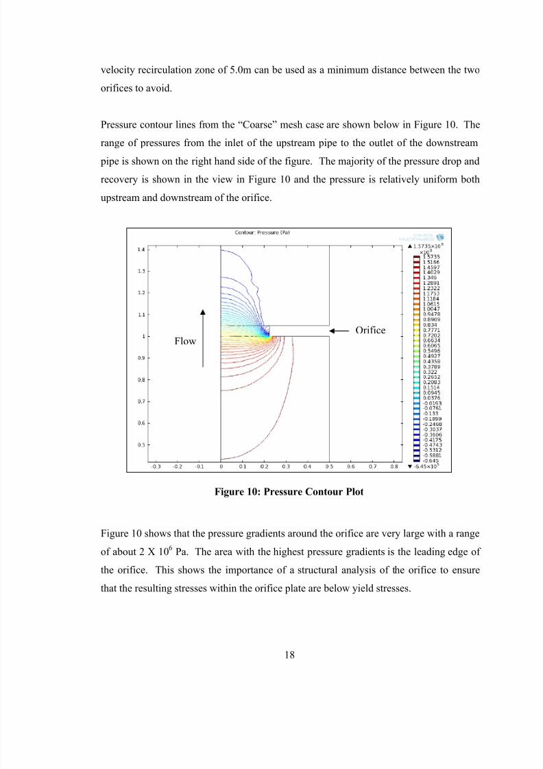
Pressure contour lines from the “Coarse” mesh case are shown below in Figure 10. The
range of pressures from the inlet of the upstream pipe to the outlet of the downstream
pipe is shown on the right hand side of the figure. The majority of the pressure drop and
recovery is shown in the view in Figure 10 and the pressure is relatively uniform both
upstream and downstream of the orifice.
Figure 10: Pressure Contour Plot
Figure 10 shows that the pressure gradients around the orifice are very large with a range
of about 2 X 10⁶ Pa. The area with the highest pressure gradients is the leading edge of
the orifice. This shows the importance of a structural analysis of the orifice to ensure
that the resulting stresses within the orifice plate are below yield stresses.
FlowOrifice
7/24/2019 DESIGN AND ANALYSIS OF ORIFICES
http://slidepdf.com/reader/full/design-and-analysis-of-orifices 26/46
19
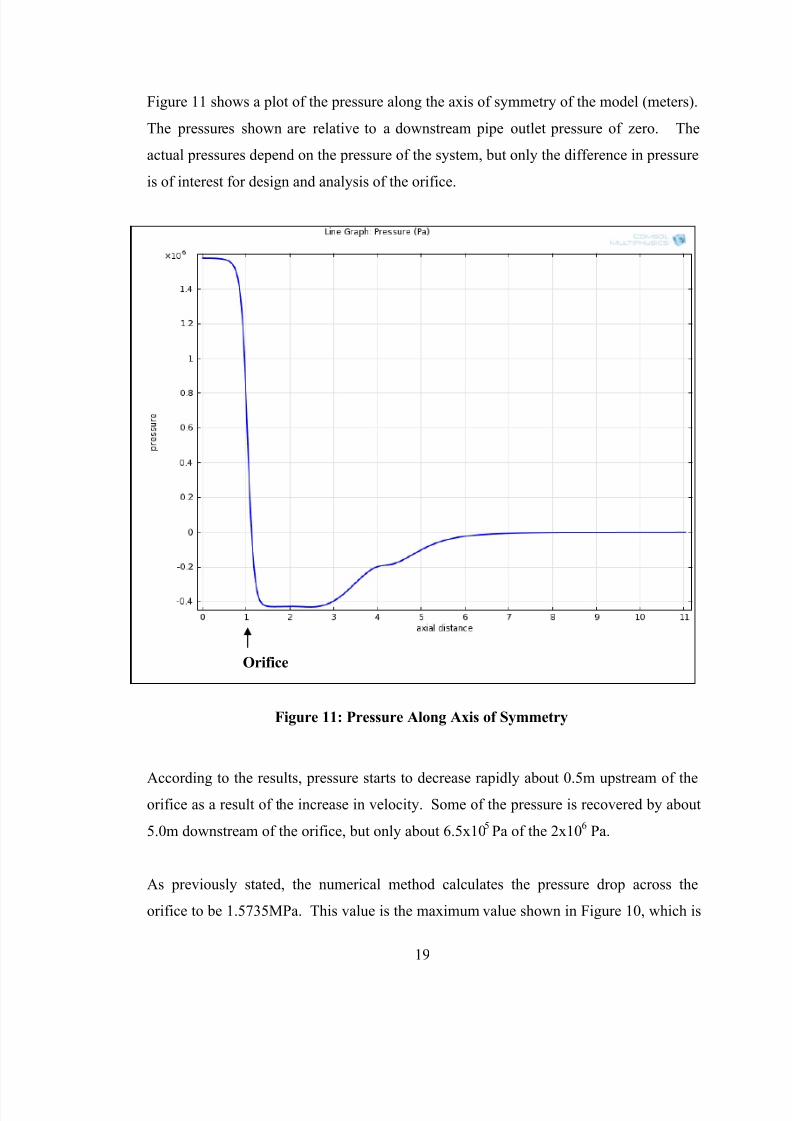
Figure 11 shows a plot of the pressure along the axis of symmetry of the model (meters).
The pressures shown are relative to a downstream pipe outlet pressure of zero. The
actual pressures depend on the pressure of the system, but only the difference in pressure
is of interest for design and analysis of the orifice.
Figure 11: Pressure Along Axis of Symmetry
According to the results, pressure starts to decrease rapidly about 0.5m upstream of theorifice as a result of the increase in velocity. Some of the pressure is recovered by about
5.0m downstream of the orifice, but only about 6.5x10⁵Pa of the 2x10
6 Pa.
As previously stated, the numerical method calculates the pressure drop across the
orifice to be 1.5735MPa. This value is the maximum value shown in Figure 10, which is
Orifice
7/24/2019 DESIGN AND ANALYSIS OF ORIFICES
http://slidepdf.com/reader/full/design-and-analysis-of-orifices 27/46
20
the maximum pressure in the system, as opposed to only the magnified view. Since the
pressures are such that the pressure value at the exit of the system, then the maximum
pressure in the system represents the total pressure drop across the orifice. COMSOL
assumes that there are no frictional losses at the pipe walls.
These results can be compared directly with the results from the analytical method from
Section 3.3. For the same geometry, flow rate and fluid properties, the two methods
calculate very different pressure drops. As stated in Section 3.3, the orifice was sized
using the analytical method to produce a pressure drop of 0.8764MPa. The difference
between the results is (1.5735-0.8764)/0.8764 = 0.795 or 79.5% of the analytical results.
The difference of 79.5% between the analytical and numerical results is much larger
than expected. This difference is attributed to the differences in equations and processes
used for calculation of the orifice pressure drop. It is thought that the analytical method
may provide the more accurate results as the equations are based on large amounts of
empirical data. However, in this case, the numerical method provides conservative input
to structural analyses that will be performed in Section 3.5.
3.5
Static Structural Analysis of Orifice
For the static structural analysis, the software ANSYS Workbench is used to determine
conservative stresses and the stress distribution throughout the geometry. This is
important to ensure that the material yield strength is not exceeded and will confirm that
the assumed orifice thickness and material is appropriate.
The geometry of the ANSYS Workbench model is identical to the orifice whose pressure
drop was determined in Sections 3.4. The outer diameter is 1.0m, the inner diameter is
0.449m and the thickness is 0.05m. This geometry is created by extruding two
concentric circles. A one-quarter slice is used for analysis purposes to reduce the
number of mesh elements required for solving. This may be done considering the
symmetrical geometry of the orifice. A one-quarter slice is chosen as the meshing for a

7/24/2019 DESIGN AND ANALYSIS OF ORIFICES
http://slidepdf.com/reader/full/design-and-analysis-of-orifices 28/46
21
one-quarter slice is simpler than it would be for a smaller slice. The geometry is shown
below in Figure 12.
Figure 12: ANSYS Workbench Geometry
Different from the method used to mesh the COMSOL model, the ANSYS auto-meshing
feature is not used. The ANSYS auto-meshing feature is not conducive to radially
symmetric geometries. To mesh the geometry, the model is manually divided so that the
elements along the edges are all uniform and all elements are of similar shape. The
entire geometry is divided along 3 edges. The number of divisions along these edges
controls the total number and size of the elements. The pattern of the meshing with large
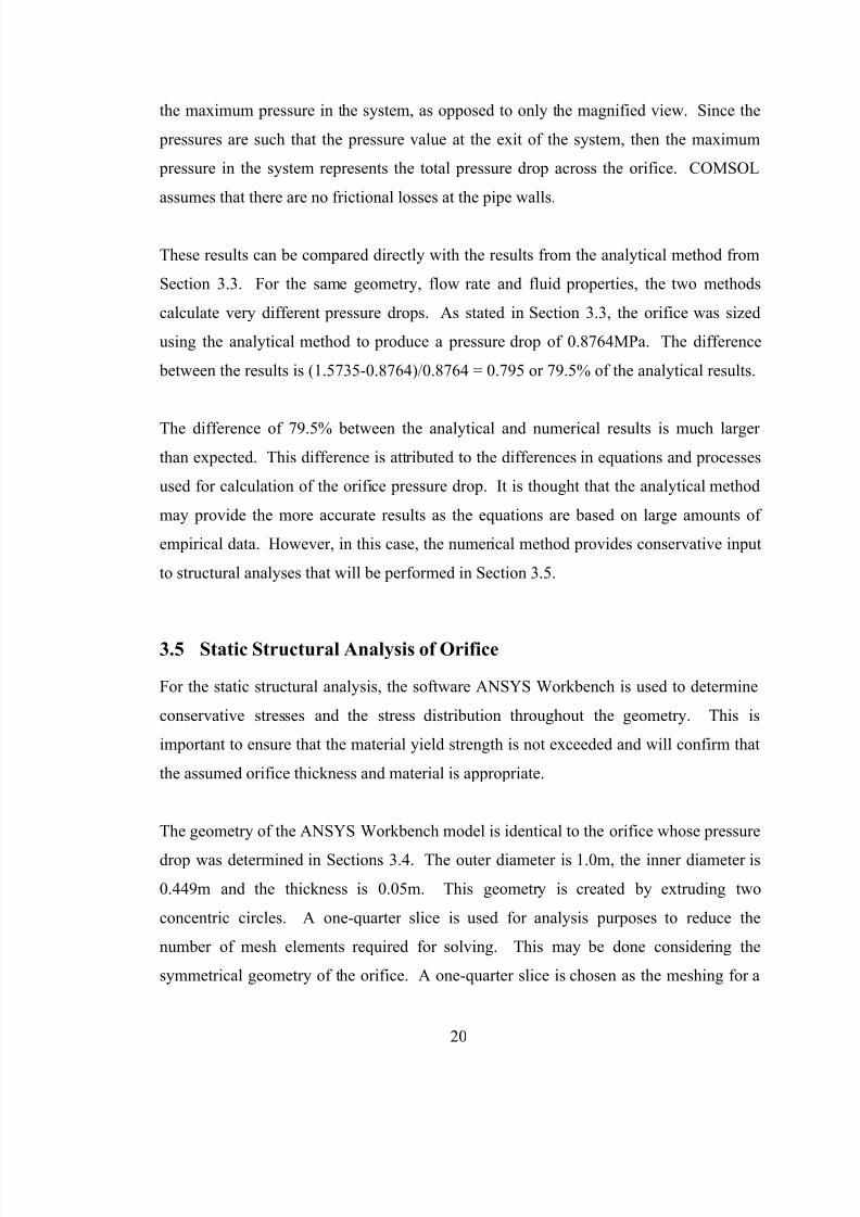
elements is shown below in Figure 13.
7/24/2019 DESIGN AND ANALYSIS OF ORIFICES
http://slidepdf.com/reader/full/design-and-analysis-of-orifices 29/46
22
Figure 13: ANSYS Workbench Model Meshing
Similar to the method used in COMSOL in Section 3.4, numerous cases are run with
different number of elements to show diminishing returns. The maximum stress
intensity is compared between each case and the results are shown in Table 2.
7/24/2019 DESIGN AND ANALYSIS OF ORIFICES
http://slidepdf.com/reader/full/design-and-analysis-of-orifices 30/46
23
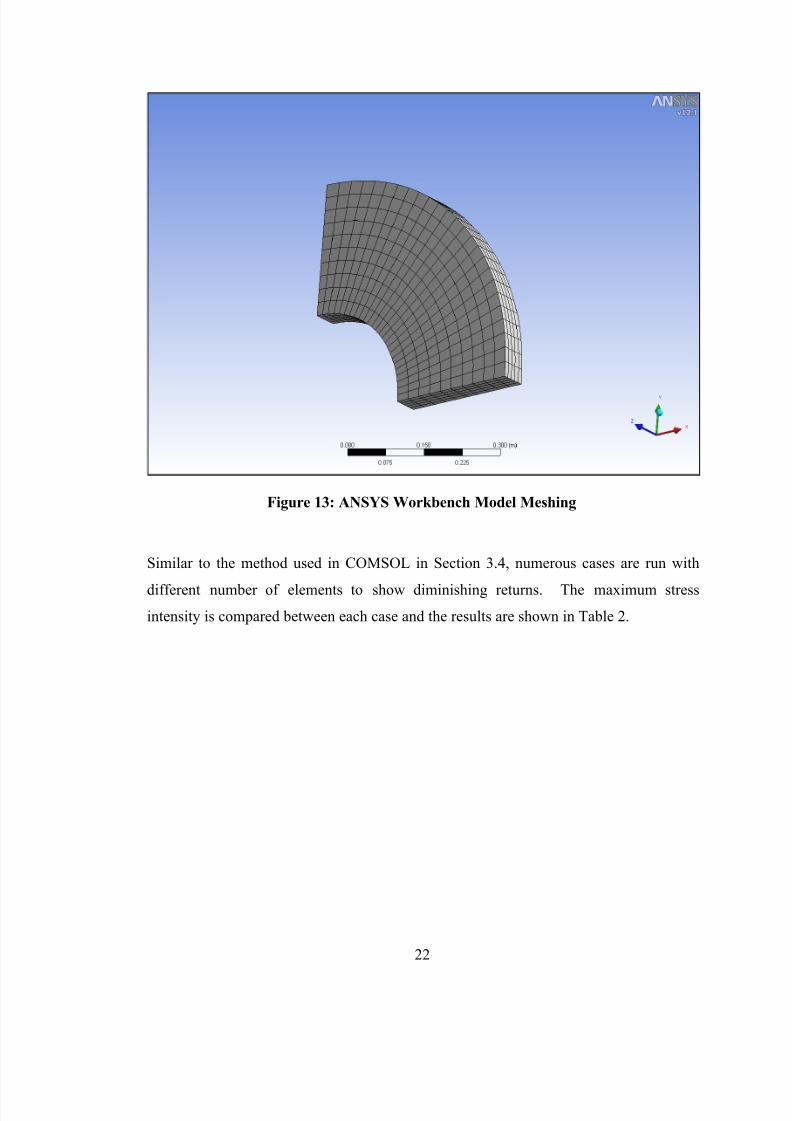
Table 2: ANSYS Mesh Comparison
ANSYS Mesh CaseTotal Number of
Elements
Maximum Stress
Intensity (MPa) Change (%)
1 1,250 82.533 N/A
2 4,480 92.299 11.8
3 10,584 100.82 9.2
4 21,315 108.73 7.8
5 43,660 117.12 7.7
6 81,000 124.31 6.1
ANSYS Mesh Case 6 is considered adequate considering the 6.1% change in maximum
stress intensity when 37,340 elements are added. Increasing the number of elements
significantly to more than 81,000 is considered not worth the extra computational time.
To obtain conservative stresses, conservative forces (or pressures) must be applied to the
model. One conservative method for defining the force would be to apply the entire
head of the pump at the low flow condition to the front face of the orifice plate. This
would be a value of 1.143MPa, which was determined in Section 3.1. If only analytical
methods were used, this would be the most conservative approach. However, in this
case, a numerical approach was also used. To use the results from the numerical
method, the pressure was plotted along the face of the orifice in the COMSOL model.
This pressure is shown below in Figure 14.
7/24/2019 DESIGN AND ANALYSIS OF ORIFICES
http://slidepdf.com/reader/full/design-and-analysis-of-orifices 31/46
24
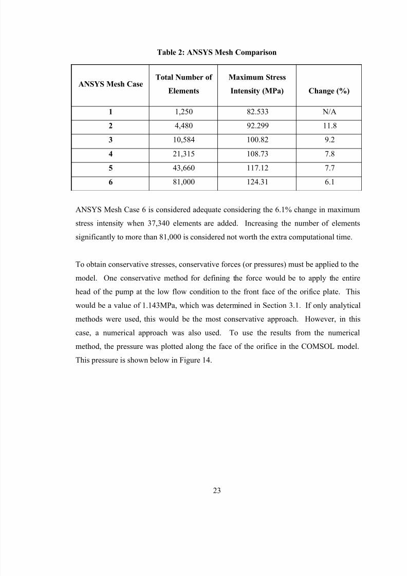
Figure 14: COMSOL Pressure Plot Along Orifice Face
According to the plot in Figure 14, the pressure increases going from the inner diameter
of the orifice to the outer diameter. From about half-way between the inner and outer
diameter to the outer diameter, the pressure is a constant 1.6MPa. This is more
conservative than the value of 1.143MPa discussed above. For simplicity and
conservatism, the pressure of 1.6MPa is applied to the entire orifice face in the ANSYS
model.
To constrain the model prior to solving, the outer edge of the orifice is a categorized as a
“Fixed Support”. This means that no translation or rotation of this surface is allowed.
This is identified as “Surface C” in Figure 15, below. This support simulates the orifice
being flanged into the surrounding piping. The cuts that are made to simplify the
geometry for symmetry are defined as “Frictionless Supports”. This allows frictionless
motion, but still provides support as if rest of the orifice is present. These surfaces are
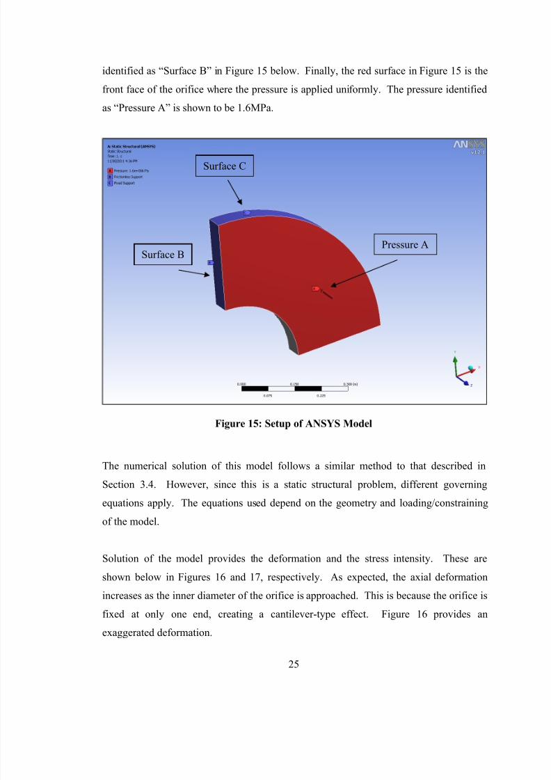
7/24/2019 DESIGN AND ANALYSIS OF ORIFICES
http://slidepdf.com/reader/full/design-and-analysis-of-orifices 32/46
7/24/2019 DESIGN AND ANALYSIS OF ORIFICES
http://slidepdf.com/reader/full/design-and-analysis-of-orifices 33/46
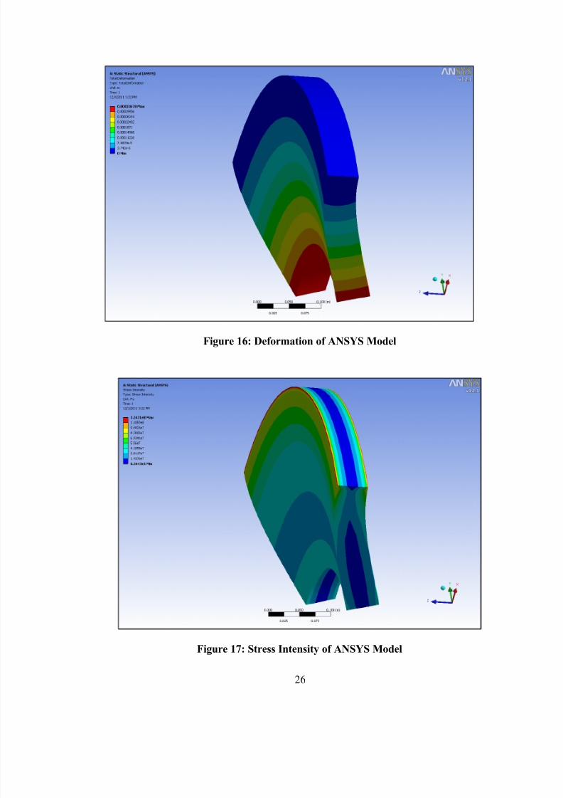
26
Figure 16: Deformation of ANSYS Model
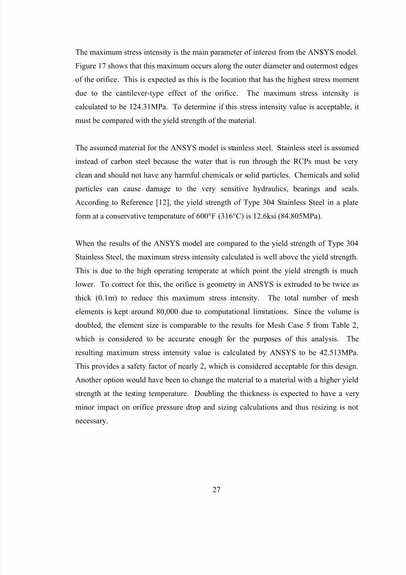
Figure 17: Stress Intensity of ANSYS Model
7/24/2019 DESIGN AND ANALYSIS OF ORIFICES
http://slidepdf.com/reader/full/design-and-analysis-of-orifices 34/46
27
The maximum stress intensity is the main parameter of interest from the ANSYS model.
Figure 17 shows that this maximum occurs along the outer diameter and outermost edges
of the orifice. This is expected as this is the location that has the highest stress moment
due to the cantilever-type effect of the orifice. The maximum stress intensity is
calculated to be 124.31MPa. To determine if this stress intensity value is acceptable, it
must be compared with the yield strength of the material.
The assumed material for the ANSYS model is stainless steel. Stainless steel is assumed
instead of carbon steel because the water that is run through the RCPs must be very
clean and should not have any harmful chemicals or solid particles. Chemicals and solid
particles can cause damage to the very sensitive hydraulics, bearings and seals.
According to Reference [12], the yield strength of Type 304 Stainless Steel in a plate
form at a conservative temperature of 600°F (316°C) is 12.6ksi (84.805MPa).
When the results of the ANSYS model are compared to the yield strength of Type 304
Stainless Steel, the maximum stress intensity calculated is well above the yield strength.
This is due to the high operating temperate at which point the yield strength is much
lower. To correct for this, the orifice is geometry in ANSYS is extruded to be twice as
thick (0.1m) to reduce this maximum stress intensity. The total number of mesh
elements is kept around 80,000 due to computational limitations. Since the volume is
doubled, the element size is comparable to the results for Mesh Case 5 from Table 2,
which is considered to be accurate enough for the purposes of this analysis. The
resulting maximum stress intensity value is calculated by ANSYS to be 42.513MPa.
This provides a safety factor of nearly 2, which is considered acceptable for this design.
Another option would have been to change the material to a material with a higher yield
strength at the testing temperature. Doubling the thickness is expected to have a very
minor impact on orifice pressure drop and sizing calculations and thus resizing is not
necessary.

7/24/2019 DESIGN AND ANALYSIS OF ORIFICES
http://slidepdf.com/reader/full/design-and-analysis-of-orifices 35/46
28
3.6 Modal Analysis of Orifices
The modal analysis is the final step to the project. The purpose of this analysis is to
determine the natural frequencies of the orifices. The supports and hydraulic forcesmust be considered. ANSYS Workbench is also used for the modal analysis so that the
same geometry and meshing can be used. Further, the supports and pre-stresses that are
calculated in the static structural analysis as a result of the hydraulic forces can be easily
applied to the geometry. Damping of the water itself and the reduction in hydraulic
force near the inner diameter of the orifice (shown in Figure 14) is considered negligible.
The first 6 natural frequencies and modes are calculated.
A modal analysis is performed on both orifices as there is not a conservative condition.
To avoid undesired resonance conditions, the natural frequencies for either orifice
cannot be the same frequency as the hydraulic pressure pulsations generated by the
pump. The number of mesh elements used for both orifices is 8960. Due to
computational limitations, this is the highest number of mesh elements that could be
used. If the results show that the orifice natural frequencies are close to the pump
hydraulic pressure pulsation frequencies, a finer mesh is recommended. The results of
the modal analyses are shown in Table 3. All mode shapes are shown exaggerated in
Appendix A.
7/24/2019 DESIGN AND ANALYSIS OF ORIFICES
http://slidepdf.com/reader/full/design-and-analysis-of-orifices 36/46
29
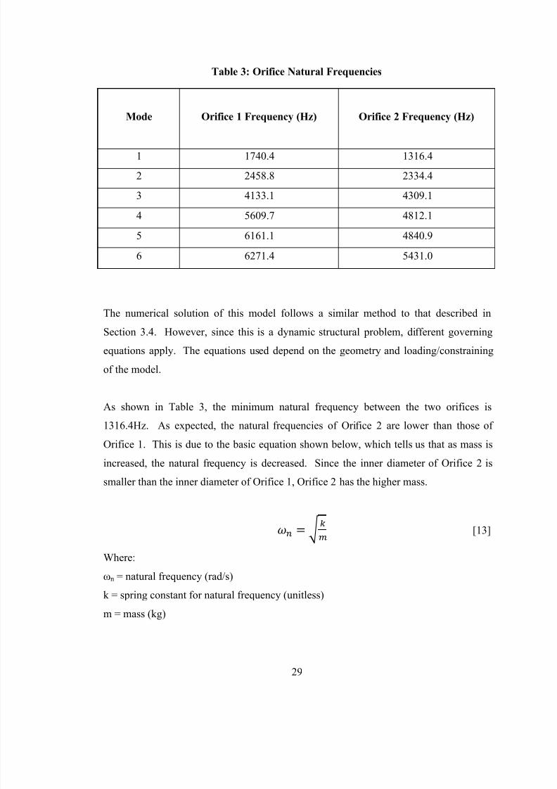
Table 3: Orifice Natural Frequencies
Mode Orifice 1 Frequency (Hz) Orifice 2 Frequency (Hz)
1 1740.4 1316.4
2 2458.8 2334.4
3 4133.1 4309.1
4 5609.7 4812.1
5 6161.1 4840.9
6 6271.4 5431.0
The numerical solution of this model follows a similar method to that described in
Section 3.4. However, since this is a dynamic structural problem, different governing
equations apply. The equations used depend on the geometry and loading/constraining
of the model.
As shown in Table 3, the minimum natural frequency between the two orifices is
1316.4Hz. As expected, the natural frequencies of Orifice 2 are lower than those of
Orifice 1. This is due to the basic equation shown below, which tells us that as mass is
increased, the natural frequency is decreased. Since the inner diameter of Orifice 2 is
smaller than the inner diameter of Orifice 1, Orifice 2 has the higher mass.
[13]
Where:
ωn = natural frequency (rad/s)
k = spring constant for natural frequency (unitless)
m = mass (kg)
7/24/2019 DESIGN AND ANALYSIS OF ORIFICES
http://slidepdf.com/reader/full/design-and-analysis-of-orifices 37/46
30
The lower mode shapes (1-3) are very similar between the two orifices since their
geometry is similar. The higher mode shapes (4-6) show some differences between the
two orifices.
A pump’s hydraulic pressure pulsation frequency is generated by the rotating impeller
blades passing by the stationary diffuser vanes. Considering, the frequency at which an
impeller blade passes a diffuser vane will be the pump pressure pulsation frequency.
This is referred to as the pump blade passing frequency (BPF). The pump speed and the
number of impeller blades determine the frequency. The impeller described by
Reference [7] is a six bladed impeller that rotates at 1190rpm.
1190rpm X 6 blades = 7,140 blade passings per minute
7,140 / 60 seconds per minute = 119Hz
The pump BPF is calculated to be 119Hz. When compared to the results in Table 3, the
pump BPF is significantly lower than the minimum orifice natural frequency of
1316.4Hz. A factor of safety of nearly 11 is achieved. With such a high factor of safety,
further analysis with finer meshing is not required. Finally, this means that the orifices
will not be excited by the pump pressure pulsations and that the orifice design is
sufficient.
7/24/2019 DESIGN AND ANALYSIS OF ORIFICES
http://slidepdf.com/reader/full/design-and-analysis-of-orifices 38/46
31
4. Conclusions
The results of this project have proved to be intriguing and thought provoking. From
Section 3.1, it was determined that the pressure drops required of the orifices are as large
as 1.143MPa (165.8psi). This emphasizes the need for two orifices rather than one asthe significant constrictions to the flow would be minimized for orifice structural
concerns and for RCP NPSH testing.
Sections 3.2 and 3.3 perform the sizing of the orifices using the analytical method, which
is generally thought to be an accurate method as the equations are derived from decades
of empirical data. The results show that Orifice 2 has the smaller inner diameter and
greatest pressure drop. The maximum pressure drop is calculated to be 876,435Pa and
occurs during the low flow condition of 7.672m3/s. This is the most limiting condition
from a structural perspective and is used for input into the structural analyses.
Results from the numerical method for calculation of the orifice pressure drop were
79.5% greater than the analytical method. This is considered to be a very poor
correlation between the two methods. The difference is attributed to the differences in
basic equations and how the equations were developed. The most conservative method
should be used for structural input and the method believed to be most accurate should
be used for sizing purposes.
Another conclusion that can be drawn from the COMSOL results is the minimum
distance between the two orifices. It is desirable to have the velocity fully recovered
from the first orifice before entering the second to avoid undesirable flow characteristics,
which could affect flow measurements. Since Orifice 2 is the more constrictive orifice
and the low flow condition is modeled, the length of the velocity recirculation zone of
5.0m can be used as a minimum distance between the two orifices to avoid.
From the structural analysis, the results showed that the maximum stress exceeded the
yield strength of Type 304 Stainless Steel for the orifice thickness of 0.05m. An orifice
of this thickness would be expected to plastically deform at the outer edges of the outer
7/24/2019 DESIGN AND ANALYSIS OF ORIFICES
http://slidepdf.com/reader/full/design-and-analysis-of-orifices 39/46
32
diameter of Orifice 2 at the low flow condition. When the thickness was increased to
0.1m, the results were found to be acceptable with a factor of safety of 2. It is concluded
that increasing the thickness of the orifice plate is a simple way to decrease the
maximum stress intensity. This is preferable to using a material with a higher yield
strength because Type 304 Stainless Steel is readily available and is most likely cheaper
than higher strength materials.
From the results of the modal analysis, it is concluded that the natural frequencies are far
above the pump pressure pulsation frequency. As a result, excitation of the orifices by
the pump pressure pulsations is not of concern.
Future studies should attempt to get a better correlation between analytical and
numerical pressure drop calculation results. A better correlation could result in more
accurate (less conservative) input to the structural analysis. This could result in a thinner
orifice plate, saving cost of material and making installation in & removal from the test
loop easier.
Future studies may also improve the meshing of the orifice for both the static and
structural analyses. A computer system with more memory would allow solving of the
geometry with more mesh elements. A smaller symmetrical section of the orifice could
also be used to reduce computational efforts. Finally, now that it is known where the
highest stress gradients are in the orifice, the mesh efficiency could be improved to have
smaller mesh elements near the orifice outer diameter and larger mesh elements near the
orifice inner diameter.
7/24/2019 DESIGN AND ANALYSIS OF ORIFICES
http://slidepdf.com/reader/full/design-and-analysis-of-orifices 40/46
33
5. References
1) “Pressurized Water Reactor (PWR) Systems”, Nuclear Regulatory Commission website
http://www.nrc.gov/reading‐rm/basic‐ref/teachers/04.pdf
2)
“Pressurized Water
Reactor
(PWR)”
Copyright
©
1996
‐2006,
The
Virtual
Nuclear
Tourist,
December 19, 2005. http://www.nucleartourist.com/type/pwr.htm
3) “Damages by Cavitation” Chemical & Process Technology, May 7, 2008.
http://webwormcpt.blogspot.com/2008/05/damages‐by‐cavitation.html
4) “Fundamentals of Fluid Mechanics”, Fifth Edition by Munson, Young and Okiishi. Copyright ©
2006 by John Wiley & Sons, Inc.
5)
“Diffuser” © 2011 Construction, Mechanical Engineering, Automotive News Tips
http://constructionmechanical‐engineering.blogspot.com/2010/04/diffuser.html
6) “Handbook of Hydraulic Resistance” Third Edition, by Idelchick, Jaico Publishing House © CRC
Press, Inc. & © Begell House Inc. First Jaico Impression: 2003, Sixth Jaico Impression: 2008
7)
Doosan Heavy
Industries
and
Construction
–
Business
Sector,
“APR1400
Class
Reactor
Coolant
Pump,”
http://www.doosan.com/doosanheavybiz/en/services/power/power_plant/reactor_coolant_p
umps.page
8) “Flow of Fluids Through Valves, Fittings, and Pipe – Technical Paper 410” © 1976 – Crane Co.
9)
“Water – Thermal Properties” The Engineering Toolbox.
http://www.engineeringtoolbox.com/water‐thermal‐properties‐d_162.html
10) “Reactor Cooling Systems… More” Copyright © 1996‐2006, The Virtual Nuclear Tourist,
January 6, 2006. http://www.nucleartourist.com/systems/rcs2.htm
11)
“An Introduction to Computational Fluid Dynamics – The Finite Volume Method” Second
Edition, H
K Versteeg
&
W
Malalasekera.
©
2007
by
Pearson
Education
Limited.
12) 2007 ASME Boiler & Pressure Vessel Code Section II, Part D “Properties – Materials”, © 2007 by
The American Society of Mechanical Engineers.
13) “Engineering Vibration” Section Edition, Daniel J. Inman. ©2001 by Prentice‐Hall, Inc.

7/24/2019 DESIGN AND ANALYSIS OF ORIFICES
http://slidepdf.com/reader/full/design-and-analysis-of-orifices 41/46
34
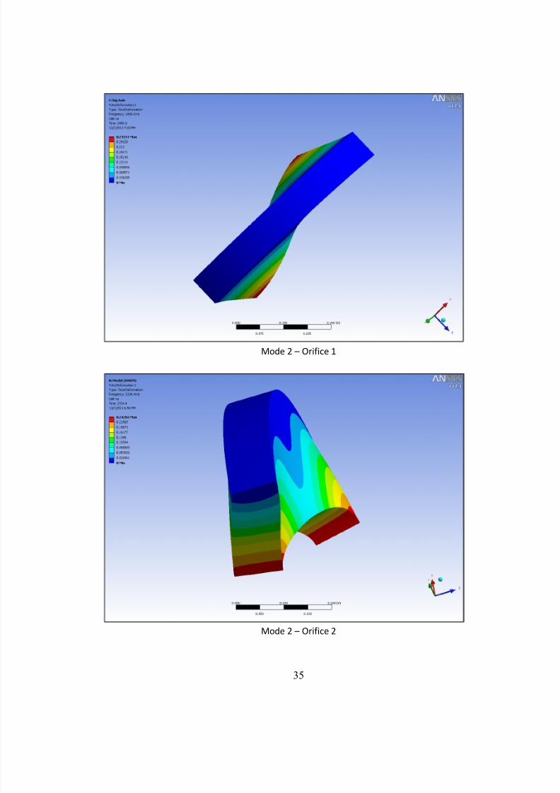
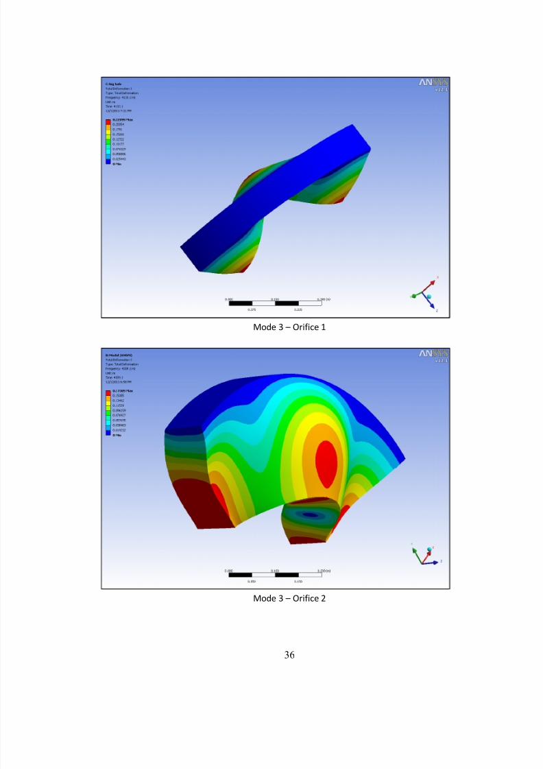
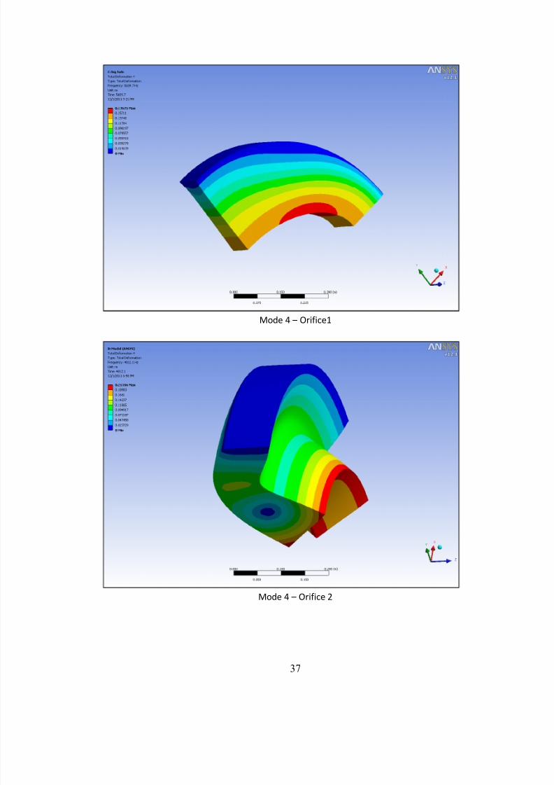
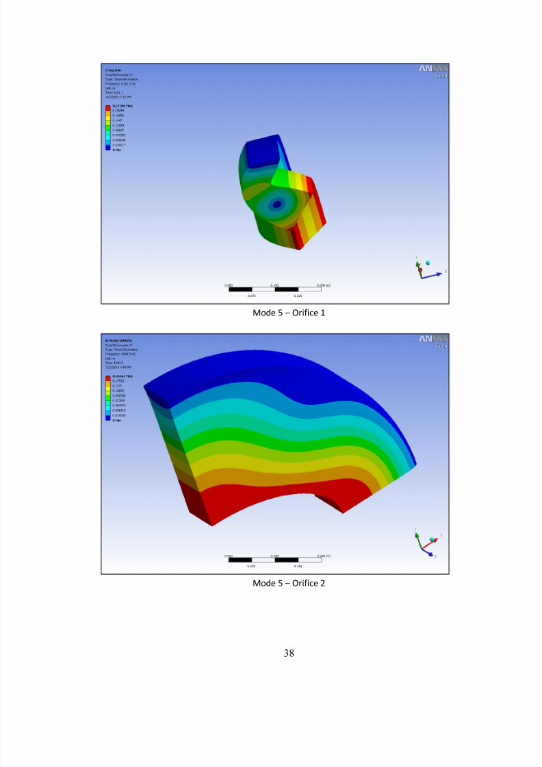
Appendix A: Orifice Mode Shapes
Mode 1 – Orifice 1
Mode 1 – Orifice 2
7/24/2019 DESIGN AND ANALYSIS OF ORIFICES
http://slidepdf.com/reader/full/design-and-analysis-of-orifices 42/46
35
Mode 2 – Orifice 1
Mode 2 – Orifice 2
7/24/2019 DESIGN AND ANALYSIS OF ORIFICES
http://slidepdf.com/reader/full/design-and-analysis-of-orifices 43/46
36
Mode 3 – Orifice 1
Mode 3 – Orifice 2
7/24/2019 DESIGN AND ANALYSIS OF ORIFICES
http://slidepdf.com/reader/full/design-and-analysis-of-orifices 44/46
37
Mode 4 – Orifice1
Mode 4 – Orifice 2
7/24/2019 DESIGN AND ANALYSIS OF ORIFICES
http://slidepdf.com/reader/full/design-and-analysis-of-orifices 45/46
38
Mode 5 – Orifice 1
Mode 5 – Orifice 2
7/24/2019 DESIGN AND ANALYSIS OF ORIFICES
http://slidepdf.com/reader/full/design-and-analysis-of-orifices 46/46
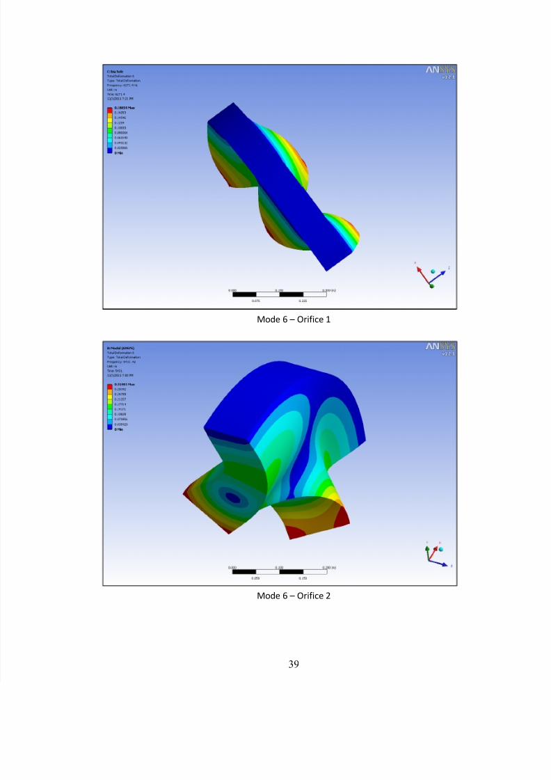
Mode 6 – Orifice 1
Mode 6 – Orifice 2