1

Pressure Drop Across Orifices in Microchannels

Febe Kusmanto ChemE 499 Spring 2003

2

The purpose of doing this paper is to show that Navier-Stokes equation is still able to predict the effect of the thickness of the orifice with orifice diameter as small as 8

microns.

Introduction:

A controversy was found in the literature between Hasegawa1 and Dagan2 papers. In

Hasegawa paper, measurements of the pressure drop across orifices for laminar flow

were done in an aperture diameter as small as 8 microns. They report that the Navier-

Stokes equation cannot predict their results, which show an effect of the thickness of the

orifice plate. However, Dagan paper mentioned that there is an analytical solution of the

Navier-Stokes equation that shows the thickness of the orifice plate is important at very

small Reynolds number.

Figure 1. The three dimensional orifice and the approximation using two dimensional, axi-symmetric.

3

When the flow is laminar, the excess pressure drop (Δp) across orifices can be

obtained by taking the pressure difference between the total pressure drop necessary to

eject the fluid through the aperture and the pressure drop that would exist if only losses

from fully developed flow was present1. The formula is represented as following:

Re2 1

22

KKUp

+=Δ

ρ (1)

where U = mean velocity ρ = density K1 and K2 = constants

µρUD

=Re = Reynolds number

µ = viscosity D = aperture diameter

Experiments from Hasegawa, et al.:

In Hasegawa1 experiment, the excess pressure drops were measured for flow

through very small orifices whose diameter ranges from 1 mm to 10µm using water,

silicon oils, and solutions of glycerin in water. The velocities were measured along the

centerline of the orifice. They stated that for larger orifices, their experimental excess

pressure drops were the same as the numerical analysis of Newtonian flow, but for

smaller orifices, the experimental results were higher. In addition, they calculated both

theoretical and numerical values of K’ as 37.7 and 27 respectively for an infinitely thin

orifice in the creeping flow; these results were experimentally confirmed. Therefore, they

concluded that Navier-Stokes could not be used to predict the effect of orifice thickness

in microchannels.

4

Figure 2. The experimental results taken from Hasegawa1 for different L/D ratio. The experiment was done using water, silicon oils, and solutions of glycerin in water. This plot was reproduced from Hasegawa1.

Figure 3. Numerical solution done by Hasegawa. Note here that they only have one numerical solution for different L/D ration. This plot was reproduced from Hasegawa1.

5

First Evidence from Dagan, et al.:

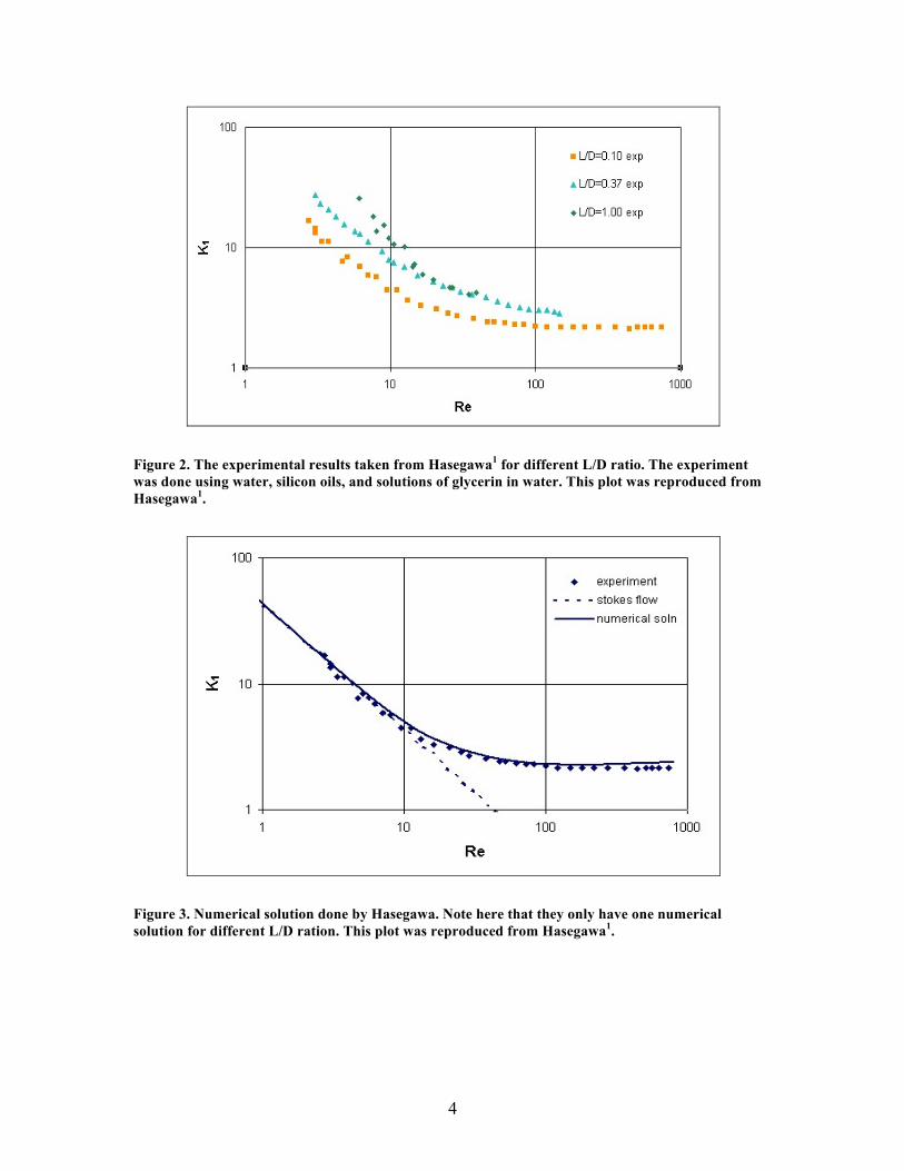
The analytical solution from Dagan2 was performed using Stokes flow (i.e. exact

solution slow flow), of which valid only for flow at low Reynolds number.

Re12

Re64

Up22

πρ

+=Δ

DL (2)

where ρ = density U = average velocity L = length of orifice D = diameter of orifice

Figure 4. The first evidence from analytical solution using exact solution slow flow. The equation used to get the analytical solution, called JFM, was taken from Dagan2.

Figure 4 above shows that pressure drop calculated using the Stokes flow follows

the experiment data at low Re. It means that Navier Stokes is able to predict the effect of

the orifice thickness at microchannels.

6

Numerical Solution from FEMLAB:

Simulation was performed in FEMLAB to get numerical solutions of the excess

pressure drop. Numerical solution of K1 and Stokes flow K1 were calculated using

FEMLAB, which has a built-in dimensionless Navier Stokes equation:

cccccc UpUU 2c . ∇+−∇=∇ µρ (3)

where ρc = density Uc = average velocity

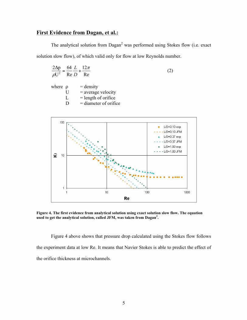
The geometry and dimension used in FEMLAB are described in the following:

Figure 5. The model and dimension used in FEMLAB simulation. To get various result at different L/D ratio, the orifice diameter (D) was kept constant while changing the orifice thickness (L). A fully developed flow was introduced at the entrance of the channel.

The length and diameter of the domain were not given in Hasegawa1’s letter.

Thus, for this calculation the length and diameter of the domain was defined as Dtube=3

and Ltube=8. In addition, to get more precise results, the calculations were also done using

7

mesh and refined mesh. The effect of domain’s diameter and length as well as mesh and

refined mesh would be discussed more detailed later.

As a result, a plot of K1 vs. Re was obtained at different L/D ratio and compared

with the experimental as well as JFM results:

Figure 6. The dimensionless Δp (K1) from FEMLAB simulation was plotted against Re for different L/D ratio. At low Re, K1 decreased as the increasing of Re and starts to level off at high Re.

According to the plot above, the calculation follows both experiment and JFM

results. At low Re, the pressure drop decreases with the increasing of Re and starts to

level off at higher Re.

Mesh refinement was also done in order to get more precise results. The following

table shows some calculations done using mesh and refined mesh at a certain L/D value.

8

Table 1. Comparison of Δp from mesh and refined mesh simulation at L/D=1. The difference between the two are really small and thus negligible.

L/D 1

Mesh Refine

Re Δpmesh Δprefine % difference

1 49.81 50.24 0.864

5 50.59 50.96 0.738

10 53.20 53.38 0.340

30 74.32 74.60 0.385

50 98.44 93.78 4.73

100 160.34

Since the difference of the calculated Δp between mesh and refine mesh

approximations is less than 1% for Reynolds number less than 50 and around 5% for

Reynolds number bigger than 50. Since the interest of the calculation is only at low

Reynolds number, so the effect of mesh refinement can be negligible.

Another assumption was that all of those calculations were done using Dtube =3

and Ltube=8. To account the effect of tube’s diameter, other calculations were done at

different tube. The calculations are shown in the following:

9

Table 2. The Δp for different tube/domain diameter. The difference among different diameter was small and thus negligible. The calculation was performed at Re = 10 and L/D = 0.37.

Re 10

L/D 0.37

dtube Δp %difference

2 33.8768 0.000

3 34.0688 0.567

4 34.0774 0.592

Based on the table above, the difference of the calculation using different tube’s

diameter values is less than 1%. Thus, the effect of tube’s diameter is negligible. Analog

to the tube’s diameter, the effect of tube’s length is also negligible.

The Effect of Domain’s Length on the Orifice Pressure Drops:

At higher L/D ratio, as Re gets bigger, the domain should be set to be long enough

to get a fully developed flow. To check for that, the exit velocity profile and pressure at

the centerline should be observed. A hyperbolic velocity profile should be appeared at the

channel exit and there should not be a negative pressure at the centerline if not the

domain’s length should be extended. For L/D = 1.14, the domain’s length should be

extended starting at Re = 200 to get a valid solution of K1.

10

Figure 7. All results at different L/D ratio each for Hasegawa experiment result (exp, points), Dagan analytical solution (JFM, dotted line) , and numerical solution using FEMLAB (calc, solid line). Note that at high Re, for high L/D ratio, the FEMLAB solution starts to deviate from what they supposed to be.

Figure 8. The exit velocity for L/D = 1.14 at Re = 200. It shows that the profile was not hyperbolic, means the velocity at the exit of the channel was not fully developed.

11

Figure 9. The results after the domain length was made longer to get fully developed velocity along the domain. Notice that at Re > 200, the domain should be made longer to get fully developed velocity along the domain.

Figure 10. The exit velocity profile for L/D = 1.14 and Re = 200 after the domain was made longer. Here, the fully developed velocity was obtained along the domain.

12

Conclusions: As conclusions, Navier-Stokes can still be used to predict the effect of the orifice

thickness to the pressure drop across micro orifices. Hasegawa1 misinterpreted the

analytical solution of Dagan2 and got incorrect numerical solution of the pressure drop at

different L/D ratio.

From the simulation and theory from Dagan2, we can get a conclusion that Navier

Stokes is still able to predict the effect of the orifice thickness to the pressure drop across

micro orifices with diameter as small as 8 microns.

At higher Re, especially for higher Re, the domain should be long enough to get

fully developed velocity.

References:

1 Hasegawa, T., M. Suganuma, and H. Watanabe, "Anomaly of excess pressure drops of the flow through very small orifices" Phys. Fluids 9, 1-3, (1997).

2 Dagan, Z., S. Weinbaum, R. Pfeffer, "An infinite-series solution for the creeping motion

though an orifice of finite length," J. Fluid Mech. 115 505-523 (1982).

13

Appendix:

Model.mat a FEMLAB model for shorter domain (L=8). This model was set at L/D =

1.14 and solving for parametric solution Rexp = 0.1:0.1:3

Longer.mat a FEMLAB model for shorter domain (L=80). This model was set at L/D

= 1.14 and solving for parametric solution Rexp = 0.1:0.1:3