Modeling, design and control of an individual wheel actuatedbrake systemCitation for published version (APA):van Duifhuizen, B. A. P., Hobo, P. D., Nijmeijer, H., & Khajepour, A. (2014). Modeling, design and control of anindividual wheel actuated brake system. (D&C; Vol. 2014.052). Eindhoven University of Technology.

Document status and date:Published: 01/01/2014

Document Version:Publisher’s PDF, also known as Version of Record (includes final page, issue and volume numbers)

Please check the document version of this publication:

• A submitted manuscript is the version of the article upon submission and before peer-review. There can beimportant differences between the submitted version and the official published version of record. Peopleinterested in the research are advised to contact the author for the final version of the publication, or visit theDOI to the publisher's website.• The final author version and the galley proof are versions of the publication after peer review.• The final published version features the final layout of the paper including the volume, issue and pagenumbers.Link to publication

General rightsCopyright and moral rights for the publications made accessible in the public portal are retained by the authors and/or other copyright ownersand it is a condition of accessing publications that users recognise and abide by the legal requirements associated with these rights.

• Users may download and print one copy of any publication from the public portal for the purpose of private study or research. • You may not further distribute the material or use it for any profit-making activity or commercial gain • You may freely distribute the URL identifying the publication in the public portal.

If the publication is distributed under the terms of Article 25fa of the Dutch Copyright Act, indicated by the “Taverne” license above, pleasefollow below link for the End User Agreement:www.tue.nl/taverne

Take down policyIf you believe that this document breaches copyright please contact us at:openaccess@tue.nlproviding details and we will investigate your claim.

Download date: 21. Jul. 2020

Modeling, Design and Control ofan Individual Wheel Actuated

Brake System

B.A.P. van Duifhuizen & P.D. Hobo

DC 2014.052

Traineeship report

Coach(es): PhD PEng. A. Khajepour (UW)dr. A. Kasaiezadeh (UW)

Supervisor: prof. dr. H. Nijmeijer (TU/e)

Technische Universiteit EindhovenDepartment Mechanical EngineeringDynamics and Control Group

Eindhoven, December, 2014

Preface

This project focuses on the modelling, designing and controlling of an individual elec-trical brake system. Such a brake-by-wire system should be more redundant, safer andless complex than current hydraulic systems. This research is done during our intern-ship at the department of vehicle dynamics at the University of Waterloo, Canada (UW).Besides this brake-by-wire system this department is also busy with the development ofhybrid powertrains (electric and air hybrid engines), component sizing and power manage-ment design through concurrent optimization, vehicle modeling through real-time simula-tion and hardware-in-the-loop, active and adaptive suspension systems, and vehicle stability(http://resonance.uwaterloo.ca/p/research_areas/).

During our internship, we gained a lot of new knowledge with respect to vehicle dy-namics, Matlab and different control methods. We also had the chance to combine currentknowledge with new matter in a working prototype, used for real-time experiments. Basedon our results we concluded that setting up a working prototype is complex due to manyuncertainties that had to be anticipated on. This research would not have been possiblewithout the help of the following people:

• Firstly, we want to thank PhD PEng. Amir Khajepour for all the help and for theopportunity to perform our internship at UW;

• Secondly, we want to thank dr. Alireza Kasaiezadeh, for all the guidance with respectto the theoretical part of the project, Kevin Cochran and Jeff Graansma, for answeringall our practical questions and for the help (and the fun stories) in the vehicle labduring our experiments;

• Furthermore, we would like to thank Laaleh Durali for sharing her knowledge on thespecific matter;

• And last but not least, we want to thank prof. Henk Nijmeijer for being our supervisorand for bringing us in contact with Amir Khajepour.

B.A.P. van Duifhuizen & P.D. Hobo

Eindhoven, December, 2014

i

ii

Abstract

The aim of this internship is to design and control a novel, compact and redundant, elec-trical brake system, which can be applied for individual wheel brake action. The resultingprototype can be implemented in a Chevrolet Equinox to increase the vehicle stability bymeans of differential braking. To check the performance and robustness of the system andits controller, a prototype brake system is designed. To design and control the brake sys-tem optimally, simulations and numerical calculations are performed in order to determinethe lay-out, components and controllers. First, the different components are determinedafter which corresponding equations of motion are made. With the use of these equations aSimulink model is built up, which is finally implemented in different types of controllers, insimulations and real-time experiments. For these experiments the prototype is incorporatedin a practical measurement set-up. The real-time measurements with respect to parameteridentification and control possibility are executed and compared to the simulation results.To conclude, the results in the simulations are promising, but the experimental results showthat a follow-up research is required in order to study it more extensively.

iii

iv

Nomenclature

AbbreviationsSymbol DescriptionABS Anti-lock Braking SystemTCS Traction Control SystemESP Electronic Stability ControlECU Engine Control UnitSBC Sensotronic Brake ControlECB Electronically Controlled BrakeFBD Free Body DiagramEOM Equations of MotionPID Proportional Integral DerivativeSMC Sliding Mode Control

v

vi

Contents

Preface ii

Abstract iv

Nomenclature vi

Contents vi

1 Introduction 11.1 Context and Motivation . . . . . . . . . . . . . . . . . . . . . . . . . . . . . 11.2 Opportunities and Objectives . . . . . . . . . . . . . . . . . . . . . . . . . . 11.3 Outline . . . . . . . . . . . . . . . . . . . . . . . . . . . . . . . . . . . . . . 2

2 Literature Review 32.1 Hydraulic Brake Systems . . . . . . . . . . . . . . . . . . . . . . . . . . . . 3

2.1.1 Mechanical Hydraulic Brake Systems . . . . . . . . . . . . . . . . . 32.1.2 Electro Hydraulic Brake Systems . . . . . . . . . . . . . . . . . . . . 5

2.2 Electro Mechanical Brake Systems . . . . . . . . . . . . . . . . . . . . . . . 62.3 Discussion . . . . . . . . . . . . . . . . . . . . . . . . . . . . . . . . . . . . 7

3 Design Considerations Prior to Extensive Brake Modeling 93.1 Master Cylinder Actuation . . . . . . . . . . . . . . . . . . . . . . . . . . . . 10

3.1.1 Ball Screw versus Excenter Driven Systems . . . . . . . . . . . . . . 103.1.2 Inline Pre-load Spring . . . . . . . . . . . . . . . . . . . . . . . . . . 10

3.2 Discussion . . . . . . . . . . . . . . . . . . . . . . . . . . . . . . . . . . . . 11

4 Brake Modeling 134.1 Deriving the Equations of Motion . . . . . . . . . . . . . . . . . . . . . . . . 14

4.1.1 Caliper Reaction Force . . . . . . . . . . . . . . . . . . . . . . . . . . 144.1.2 Actuator and Pre-load Force . . . . . . . . . . . . . . . . . . . . . . . 164.1.3 Torque in the Excenter Mechanism . . . . . . . . . . . . . . . . . . . 164.1.4 Motor and Gearbox . . . . . . . . . . . . . . . . . . . . . . . . . . . 174.1.5 The Equations of Motion Completed . . . . . . . . . . . . . . . . . . 18

4.2 Discussion . . . . . . . . . . . . . . . . . . . . . . . . . . . . . . . . . . . . 18

5 Simulink Model of the Designed Brake System 195.1 Equations of Motion in a Simulink Model . . . . . . . . . . . . . . . . . . . 195.2 Simplifying and Discretizing the Simulink Model . . . . . . . . . . . . . . . 22

5.2.1 Simplification of the Model . . . . . . . . . . . . . . . . . . . . . . . 225.2.2 Discretization of the Model . . . . . . . . . . . . . . . . . . . . . . . 24

5.3 Coulomb Friction of the Motor . . . . . . . . . . . . . . . . . . . . . . . . . 255.4 Discussion . . . . . . . . . . . . . . . . . . . . . . . . . . . . . . . . . . . . 27

vii

6 Controller Design for the Brake System 296.1 PID Controller . . . . . . . . . . . . . . . . . . . . . . . . . . . . . . . . . . 29

6.1.1 Tuning Methods . . . . . . . . . . . . . . . . . . . . . . . . . . . . . 306.1.2 Gain Scheduling . . . . . . . . . . . . . . . . . . . . . . . . . . . . . 33

6.2 Sliding Mode Controller . . . . . . . . . . . . . . . . . . . . . . . . . . . . . 356.3 Discussion . . . . . . . . . . . . . . . . . . . . . . . . . . . . . . . . . . . . 37

7 Experimental Setup and Results 397.1 Experimental Setup . . . . . . . . . . . . . . . . . . . . . . . . . . . . . . . 39

7.1.1 Preliminary Experiment . . . . . . . . . . . . . . . . . . . . . . . . . 397.1.2 Component Selection . . . . . . . . . . . . . . . . . . . . . . . . . . 407.1.3 Pre-load Mechanism . . . . . . . . . . . . . . . . . . . . . . . . . . . 427.1.4 Mechanical Design . . . . . . . . . . . . . . . . . . . . . . . . . . . 427.1.5 Measurements . . . . . . . . . . . . . . . . . . . . . . . . . . . . . . 43

7.2 Experimental Results . . . . . . . . . . . . . . . . . . . . . . . . . . . . . . . 437.2.1 Openloop Parameter Identification . . . . . . . . . . . . . . . . . . . 437.2.2 PID Controlled Results . . . . . . . . . . . . . . . . . . . . . . . . . 487.2.3 SMC Controlled Results . . . . . . . . . . . . . . . . . . . . . . . . . 497.2.4 Discussion . . . . . . . . . . . . . . . . . . . . . . . . . . . . . . . . 49

8 Conclusion and Recommendations 518.1 Conclusion . . . . . . . . . . . . . . . . . . . . . . . . . . . . . . . . . . . . 518.2 Recommendations . . . . . . . . . . . . . . . . . . . . . . . . . . . . . . . . 51

Bibliography 53

Appendix A Matlab Codes Simulink Model 55A.1 Feedback Torque Function Block . . . . . . . . . . . . . . . . . . . . . . . . 55A.2 Rotational to Translational Displacement Function Block . . . . . . . . . . . 55A.3 Smooth Step Function Block . . . . . . . . . . . . . . . . . . . . . . . . . . 56

Appendix B Simulink Subsystem Blocks E.O.M. 57B.1 Eccentric mechanism E.O.M. block . . . . . . . . . . . . . . . . . . . . . . . 57B.2 Ball screw mechanism E.O.M. block . . . . . . . . . . . . . . . . . . . . . . 58

Appendix C Sliding Mode Controller 59C.1 SMC Equation . . . . . . . . . . . . . . . . . . . . . . . . . . . . . . . . . . 59C.2 Simulink model . . . . . . . . . . . . . . . . . . . . . . . . . . . . . . . . . 61

Appendix D Input Parameters 63

Appendix E Optimization of Parameters: Matlab Code 65E.1 Motor parameters . . . . . . . . . . . . . . . . . . . . . . . . . . . . . . . . 65

E.1.1 Main File . . . . . . . . . . . . . . . . . . . . . . . . . . . . . . . . . 65E.1.2 Objective Function . . . . . . . . . . . . . . . . . . . . . . . . . . . . 66

E.2 Full System Identification 1 . . . . . . . . . . . . . . . . . . . . . . . . . . . 66E.2.1 Main File . . . . . . . . . . . . . . . . . . . . . . . . . . . . . . . . . 66E.2.2 Objective Function . . . . . . . . . . . . . . . . . . . . . . . . . . . . 67E.2.3 Constraint Function . . . . . . . . . . . . . . . . . . . . . . . . . . . 68

E.3 Full System Identification 2 . . . . . . . . . . . . . . . . . . . . . . . . . . . 68E.3.1 Main File . . . . . . . . . . . . . . . . . . . . . . . . . . . . . . . . . 68E.3.2 Objective Function . . . . . . . . . . . . . . . . . . . . . . . . . . . . 69E.3.3 Constraint Function . . . . . . . . . . . . . . . . . . . . . . . . . . . 70

viii

Chapter 1

Introduction

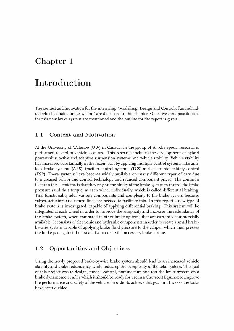
The context and motivation for the internship "Modelling, Design and Control of an individ-ual wheel actuated brake system" are discussed in this chapter. Objectives and possibilitiesfor this new brake system are mentioned and the outline for the report is given.

1.1 Context and Motivation

At the University of Waterloo (UW) in Canada, in the group of A. Khajepour, research isperformed related to vehicle systems. This research includes the development of hybridpowertrains, active and adaptive suspension systems and vehicle stability. Vehicle stabilityhas increased substantially in the recent past by applying multiple control systems, like anti-lock brake systems (ABS), traction control systems (TCS) and electronic stability control(ESP). These systems have become widely available on many different types of cars dueto increased sensor and control technology and reduced component prices. The commonfactor in these systems is that they rely on the ability of the brake system to control the brakepressure (and thus torque) at each wheel individually, which is called differential braking.This functionality adds various components and complexity to the brake system becausevalves, actuators and return lines are needed to facilitate this. In this report a new type ofbrake system is investigated, capable of applying differential braking. This system will beintegrated at each wheel in order to improve the simplicity and increase the redundancy ofthe brake system, when compared to other brake systems that are currently commerciallyavailable. It consists of electronic and hydraulic components in order to create a small brake-by-wire system capable of applying brake fluid pressure to the caliper, which then pressesthe brake pad against the brake disc to create the necessary brake torque.

1.2 Opportunities and Objectives

Using the newly proposed brake-by-wire brake system should lead to an increased vehiclestability and brake redundancy, while reducing the complexity of the total system. The goalof this project was to design, model, control, manufacture and test the brake system on abrake dynamometer after which it should be ready for use in a Chevrolet Equinox to improvethe performance and safety of the vehicle. In order to achieve this goal in 11 weeks the taskshave been divided.

1

The general goals to achieve this objective were:

• Performance of a small literature review in order to gain insights into the strengthsand weaknesses of the currently available systems;

• Design of a small and optimal brake-by-wire system with an optimal size and weight,and capacity to fully lock each wheel of the Chevrolet Equinox (≈ 12 [MPa]) within 50[ms];

• Development of a Simulink model to simulate the system behavior and performance;

• Development of a robust controller in Simulink to achieve the required performancewith a smooth pressure response;

• Development of a 3D design, CAD drawings and write a Bill Of Materials;

• Manufacture the components and assemble the prototype;

• Performance measurements on the brake dynamometer. Validation of the model bymeasuring the prototype open-loop response and identifying the system parameters;

• Performance of additional measurements to validate the controller performance androbustness to uncertainties by using challenging setpoints and varying conditions.

1.3 Outline

In Chapter 2 a brief review of the performed literature study is given. The commonly usedconventional brake systems are discussed, followed by the currently available more expen-sive brake-by-wire systems such as the electro hydraulic and electro-mechanical brake sys-tems. Chapter 3 explains some basic design considerations which have been applied priorto determining the equations of motion and the Simulink model. The EOM of the completesystem are derived in Chapter 4 subsequently a Simulink model is built in Chapter 5. Themodel behavior is identified to develop an optimal controller in Chapter 6. In Chapter 7the prototype and the used components in the experimental measurement set-up are dis-cussed. The results of the experimental measurements are displayed in Chapter 7.2, theseresults are validated with the numerical results in order to determine the accuracy and anypossible causes for deviations. Finally, conclusions and recommendations are presented inChapter 8.

2

Chapter 2

Literature Review

A literature study has been performed to create a basis for this internship. First, the in-dustry’s most commonly used hydraulic brake systems, of which some are able of applyingdifferential braking, are discussed. After this, their electro-mechanical alternatives withsimilar functionality are discussed. Finally, control strategies and controllers are presentedwhich are applied on the designed braking system.

2.1 Hydraulic Brake Systems

Hydraulic brake systems are the most commonly used type of brake systems in the auto-motive industry. In the low-end market there are the purely mechanical hydraulic systems,while in the normal to high-end market electro hydraulic systems are used. In this sec-tion, both systems are discussed with respect to their working principles, advantages anddisadvantages.

2.1.1 Mechanical Hydraulic Brake Systems

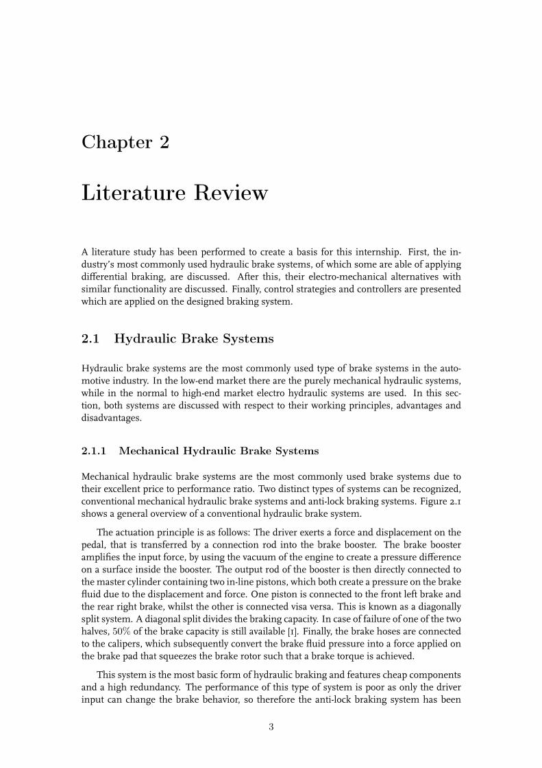
Mechanical hydraulic brake systems are the most commonly used brake systems due totheir excellent price to performance ratio. Two distinct types of systems can be recognized,conventional mechanical hydraulic brake systems and anti-lock braking systems. Figure 2.1shows a general overview of a conventional hydraulic brake system.

The actuation principle is as follows: The driver exerts a force and displacement on thepedal, that is transferred by a connection rod into the brake booster. The brake boosteramplifies the input force, by using the vacuum of the engine to create a pressure differenceon a surface inside the booster. The output rod of the booster is then directly connected tothe master cylinder containing two in-line pistons, which both create a pressure on the brakefluid due to the displacement and force. One piston is connected to the front left brake andthe rear right brake, whilst the other is connected visa versa. This is known as a diagonallysplit system. A diagonal split divides the braking capacity. In case of failure of one of the twohalves, 50% of the brake capacity is still available [1]. Finally, the brake hoses are connectedto the calipers, which subsequently convert the brake fluid pressure into a force applied onthe brake pad that squeezes the brake rotor such that a brake torque is achieved.

This system is the most basic form of hydraulic braking and features cheap componentsand a high redundancy. The performance of this type of system is poor as only the driverinput can change the brake behavior, so therefore the anti-lock braking system has been

3

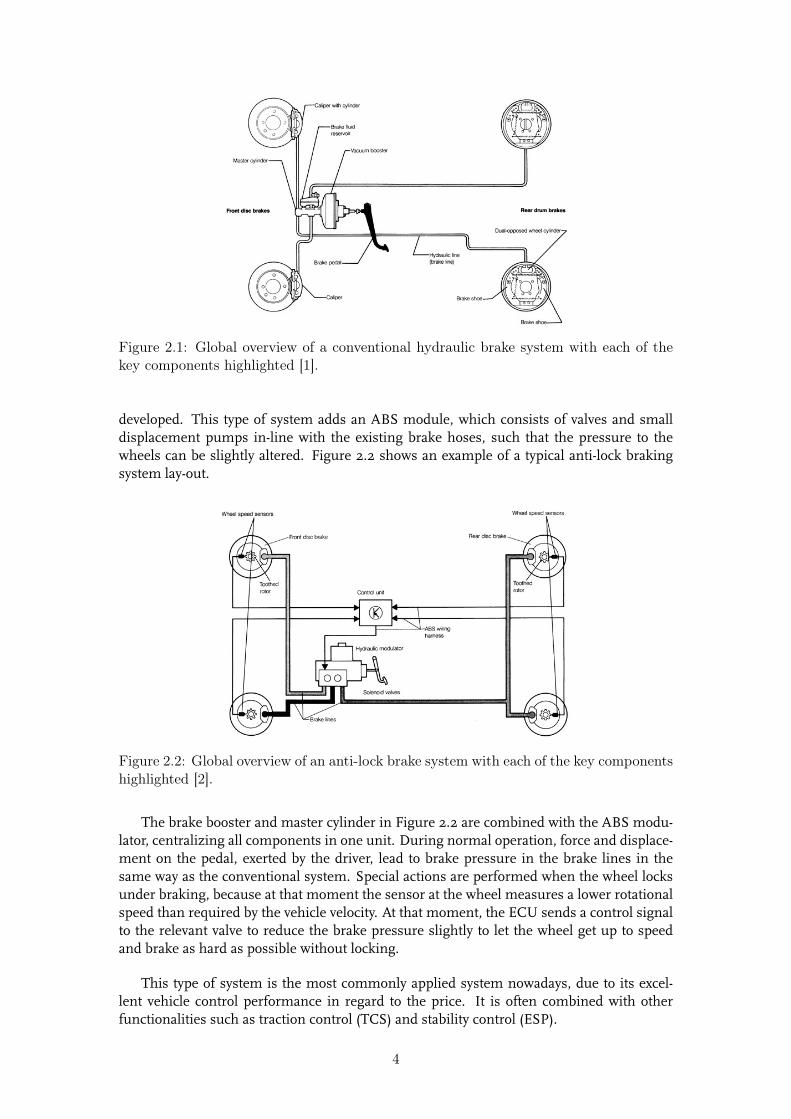
Figure 2.1: Global overview of a conventional hydraulic brake system with each of thekey components highlighted [1].

developed. This type of system adds an ABS module, which consists of valves and smalldisplacement pumps in-line with the existing brake hoses, such that the pressure to thewheels can be slightly altered. Figure 2.2 shows an example of a typical anti-lock brakingsystem lay-out.

Figure 2.2: Global overview of an anti-lock brake system with each of the key componentshighlighted [2].

The brake booster and master cylinder in Figure 2.2 are combined with the ABS modu-lator, centralizing all components in one unit. During normal operation, force and displace-ment on the pedal, exerted by the driver, lead to brake pressure in the brake lines in thesame way as the conventional system. Special actions are performed when the wheel locksunder braking, because at that moment the sensor at the wheel measures a lower rotationalspeed than required by the vehicle velocity. At that moment, the ECU sends a control signalto the relevant valve to reduce the brake pressure slightly to let the wheel get up to speedand brake as hard as possible without locking.

This type of system is the most commonly applied system nowadays, due to its excel-lent vehicle control performance in regard to the price. It is often combined with otherfunctionalities such as traction control (TCS) and stability control (ESP).

4

2.1.2 Electro Hydraulic Brake Systems

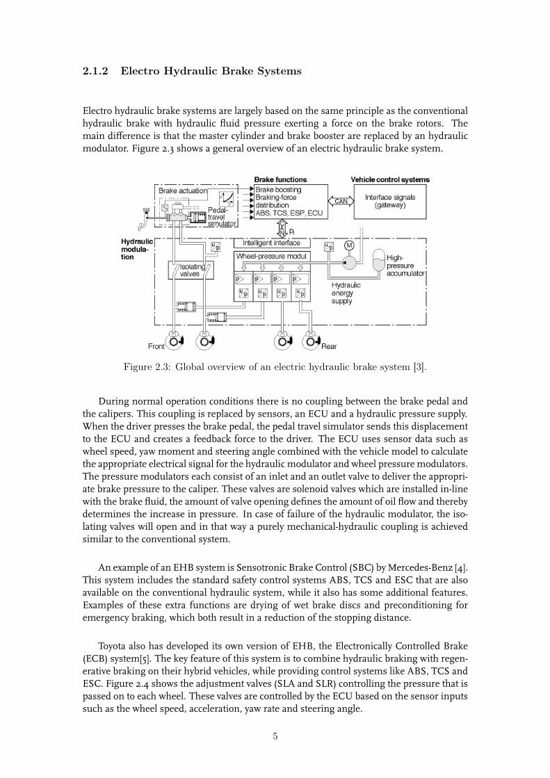
Electro hydraulic brake systems are largely based on the same principle as the conventionalhydraulic brake with hydraulic fluid pressure exerting a force on the brake rotors. Themain difference is that the master cylinder and brake booster are replaced by an hydraulicmodulator. Figure 2.3 shows a general overview of an electric hydraulic brake system.

Figure 2.3: Global overview of an electric hydraulic brake system [3].

During normal operation conditions there is no coupling between the brake pedal andthe calipers. This coupling is replaced by sensors, an ECU and a hydraulic pressure supply.When the driver presses the brake pedal, the pedal travel simulator sends this displacementto the ECU and creates a feedback force to the driver. The ECU uses sensor data such aswheel speed, yaw moment and steering angle combined with the vehicle model to calculatethe appropriate electrical signal for the hydraulic modulator and wheel pressure modulators.The pressure modulators each consist of an inlet and an outlet valve to deliver the appropri-ate brake pressure to the caliper. These valves are solenoid valves which are installed in-linewith the brake fluid, the amount of valve opening defines the amount of oil flow and therebydetermines the increase in pressure. In case of failure of the hydraulic modulator, the iso-lating valves will open and in that way a purely mechanical-hydraulic coupling is achievedsimilar to the conventional system.

An example of an EHB system is Sensotronic Brake Control (SBC) by Mercedes-Benz [4].This system includes the standard safety control systems ABS, TCS and ESC that are alsoavailable on the conventional hydraulic system, while it also has some additional features.Examples of these extra functions are drying of wet brake discs and preconditioning foremergency braking, which both result in a reduction of the stopping distance.

Toyota also has developed its own version of EHB, the Electronically Controlled Brake(ECB) system[5]. The key feature of this system is to combine hydraulic braking with regen-erative braking on their hybrid vehicles, while providing control systems like ABS, TCS andESC. Figure 2.4 shows the adjustment valves (SLA and SLR) controlling the pressure that ispassed on to each wheel. These valves are controlled by the ECU based on the sensor inputssuch as the wheel speed, acceleration, yaw rate and steering angle.

5

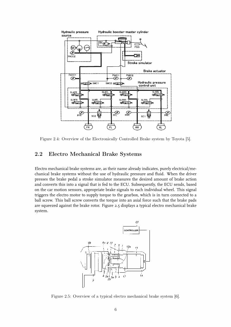
Figure 2.4: Overview of the Electronically Controlled Brake system by Toyota [5].

2.2 Electro Mechanical Brake Systems

Electro mechanical brake systems are, as their name already indicates, purely electrical/me-chanical brake systems without the use of hydraulic pressure and fluid. When the driverpresses the brake pedal a stroke simulator measures the desired amount of brake actionand converts this into a signal that is fed to the ECU. Subsequently, the ECU sends, basedon the car motion sensors, appropriate brake signals to each individual wheel. This signaltriggers the electro motor to supply torque to the gearbox, which is in turn connected to aball screw. This ball screw converts the torque into an axial force such that the brake padsare squeezed against the brake rotor. Figure 2.5 displays a typical electro mechanical brakesystem.

Figure 2.5: Overview of a typical electro mechanical brake system [6].

6

In literature the importance of the clamping force for EMB systems has been demon-strated [7]. Instead of measuring the clamping force by means of a sensor, a model is derivedwhich predicts the clamping force based on the brake pad temperature. An accurate valuefor the clamping force is of high importance for EMB’s because the pad displacement willvary by temperature, environmental conditions and wear.

2.3 Discussion

In this chapter, conventional, electro hydraulic and electro mechanical brake systems havebeen discussed. Each of the systems have their own advantages and disadvantages; TheEHB uses a hydraulic modulator and valves to feature all desired safety control systems andit has a high redundancy in case of electrical failure because a conventional backup circuitis available. All of this functionality comes at the cost of being complex and expensive tomanufacture and control. The EMB uses only electrical components making it less compli-cated and expensive, to achieve a similar safety level as the EHB system. In case of electricalfailure there is no backup circuit available to apply braking. So a conventional system iscurrently still needed to offer sufficient redundancy.

In order to combine the lower complexity of the EMB with the redundancy of the EHB,a new design for a brake system will be developed that is capable of differential braking,while remaining compatible with all the standard safety control systems such as ABS, TCSand ESC.

7

8

Chapter 3

Design Considerations Prior toExtensive Brake Modeling

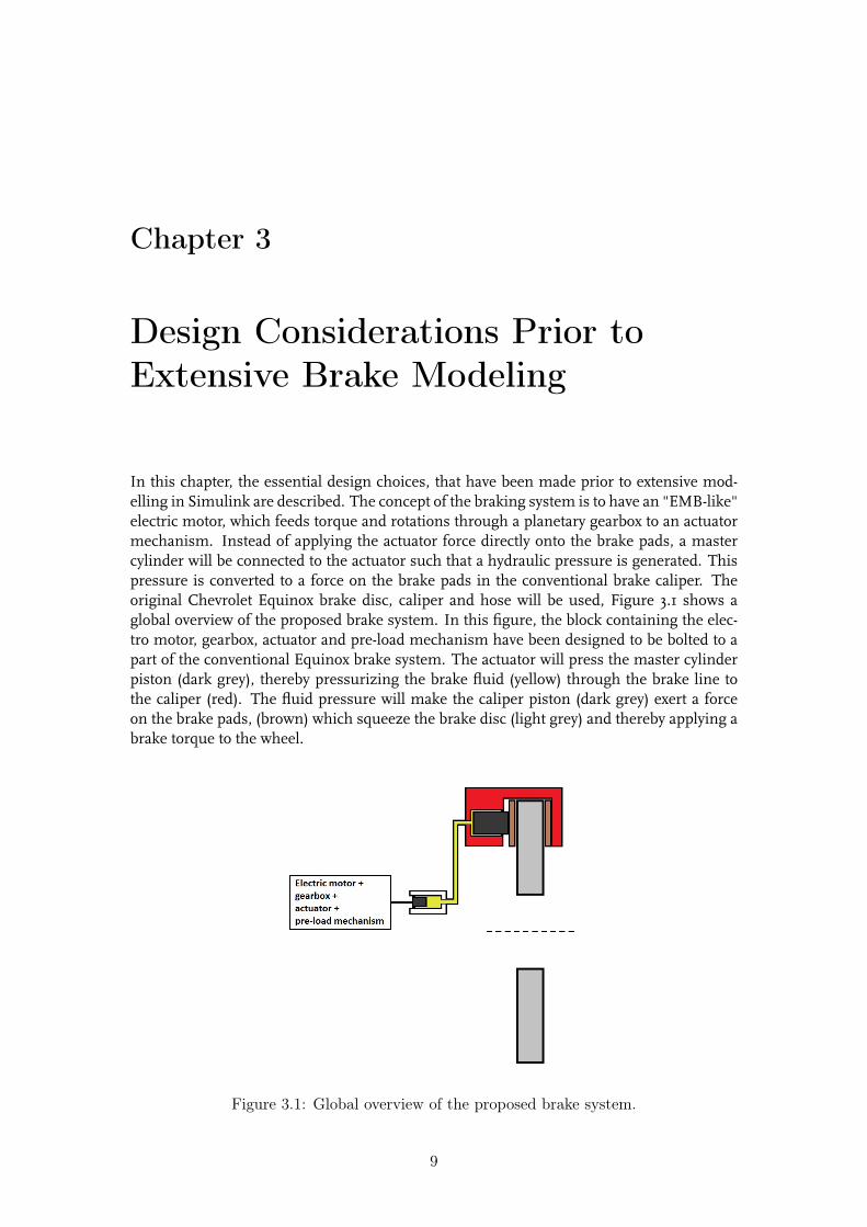
In this chapter, the essential design choices, that have been made prior to extensive mod-elling in Simulink are described. The concept of the braking system is to have an "EMB-like"electric motor, which feeds torque and rotations through a planetary gearbox to an actuatormechanism. Instead of applying the actuator force directly onto the brake pads, a mastercylinder will be connected to the actuator such that a hydraulic pressure is generated. Thispressure is converted to a force on the brake pads in the conventional brake caliper. Theoriginal Chevrolet Equinox brake disc, caliper and hose will be used, Figure 3.1 shows aglobal overview of the proposed brake system. In this figure, the block containing the elec-tro motor, gearbox, actuator and pre-load mechanism have been designed to be bolted to apart of the conventional Equinox brake system. The actuator will press the master cylinderpiston (dark grey), thereby pressurizing the brake fluid (yellow) through the brake line tothe caliper (red). The fluid pressure will make the caliper piston (dark grey) exert a forceon the brake pads, (brown) which squeeze the brake disc (light grey) and thereby applying abrake torque to the wheel.

Figure 3.1: Global overview of the proposed brake system.

9

3.1 Master Cylinder Actuation

3.1.1 Ball Screw versus Excenter Driven Systems

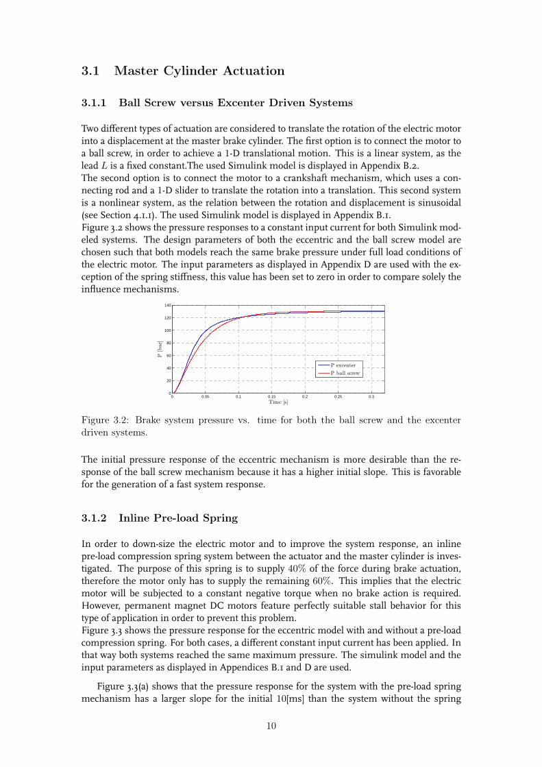
Two different types of actuation are considered to translate the rotation of the electric motorinto a displacement at the master brake cylinder. The first option is to connect the motor toa ball screw, in order to achieve a 1-D translational motion. This is a linear system, as thelead L is a fixed constant.The used Simulink model is displayed in Appendix B.2.The second option is to connect the motor to a crankshaft mechanism, which uses a con-necting rod and a 1-D slider to translate the rotation into a translation. This second systemis a nonlinear system, as the relation between the rotation and displacement is sinusoidal(see Section 4.1.1). The used Simulink model is displayed in Appendix B.1.Figure 3.2 shows the pressure responses to a constant input current for both Simulink mod-eled systems. The design parameters of both the eccentric and the ball screw model arechosen such that both models reach the same brake pressure under full load conditions ofthe electric motor. The input parameters as displayed in Appendix D are used with the ex-ception of the spring stiffness, this value has been set to zero in order to compare solely theinfluence mechanisms.

0 0.05 0.1 0.15 0.2 0.25 0.30

20

40

60

80

100

120

140

P[bar]

Time [s]

P excenter

P ball screw

Figure 3.2: Brake system pressure vs. time for both the ball screw and the excenterdriven systems.

The initial pressure response of the eccentric mechanism is more desirable than the re-sponse of the ball screw mechanism because it has a higher initial slope. This is favorablefor the generation of a fast system response.

3.1.2 Inline Pre-load Spring

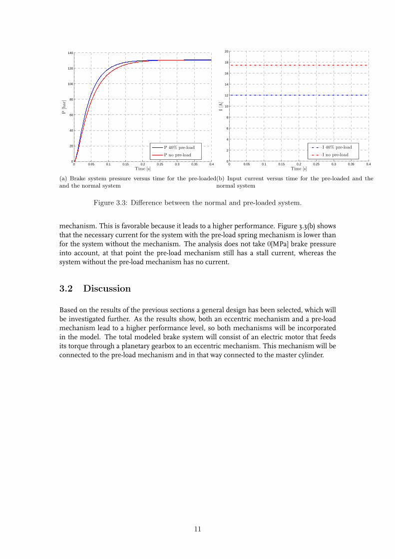
In order to down-size the electric motor and to improve the system response, an inlinepre-load compression spring system between the actuator and the master cylinder is inves-tigated. The purpose of this spring is to supply 40% of the force during brake actuation,therefore the motor only has to supply the remaining 60%. This implies that the electricmotor will be subjected to a constant negative torque when no brake action is required.However, permanent magnet DC motors feature perfectly suitable stall behavior for thistype of application in order to prevent this problem.Figure 3.3 shows the pressure response for the eccentric model with and without a pre-loadcompression spring. For both cases, a different constant input current has been applied. Inthat way both systems reached the same maximum pressure. The simulink model and theinput parameters as displayed in Appendices B.1 and D are used.

Figure 3.3(a) shows that the pressure response for the system with the pre-load springmechanism has a larger slope for the initial 10[ms] than the system without the spring

10

0 0.05 0.1 0.15 0.2 0.25 0.3 0.35 0.40

20

40

60

80

100

120

140

P[bar]

Time [s]

P 40% pre-load

P no pre-load

(a) Brake system pressure versus time for the pre-loadedand the normal system

0 0.05 0.1 0.15 0.2 0.25 0.3 0.35 0.40

2

4

6

8

10

12

14

16

18

20

I[A

]

Time [s]

I 40% pre-load

I no pre-load

(b) Input current versus time for the pre-loaded and thenormal system

Figure 3.3: Difference between the normal and pre-loaded system.

mechanism. This is favorable because it leads to a higher performance. Figure 3.3(b) showsthat the necessary current for the system with the pre-load spring mechanism is lower thanfor the system without the mechanism. The analysis does not take 0[MPa] brake pressureinto account, at that point the pre-load mechanism still has a stall current, whereas thesystem without the pre-load mechanism has no current.

3.2 Discussion

Based on the results of the previous sections a general design has been selected, which willbe investigated further. As the results show, both an eccentric mechanism and a pre-loadmechanism lead to a higher performance level, so both mechanisms will be incorporatedin the model. The total modeled brake system will consist of an electric motor that feedsits torque through a planetary gearbox to an eccentric mechanism. This mechanism will beconnected to the pre-load mechanism and in that way connected to the master cylinder.

11

12

Chapter 4

Brake Modeling

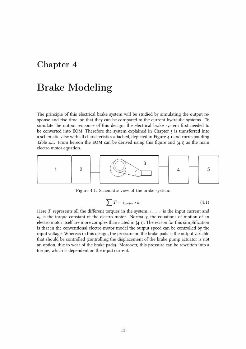
The principle of this electrical brake system will be studied by simulating the output re-sponse and rise time, so that they can be compared to the current hydraulic systems. Tosimulate the output response of this design, the electrical brake system first needed tobe converted into EOM. Therefore the system explained in Chapter 3 is transferred intoa schematic view with all characteristics attached, depicted in Figure 4.1 and correspondingTable 4.1. From hereon the EOM can be derived using this figure and (4.1) as the mainelectro motor equation.

Figure 4.1: Schematic view of the brake system.∑T = imotor · kt (4.1)

Here T represents all the different torques in the system, imotor is the input current andkt is the torque constant of the electro motor. Normally, the equations of motion of anelectro motor itself are more complex than stated in (4.1). The reason for this simplificationis that in the conventional electro motor model the output speed can be controlled by theinput voltage. Whereas in this design, the pressure on the brake pads is the output variablethat should be controlled (controlling the displacement of the brake pump actuator is notan option, due to wear of the brake pads). Moreover, this pressure can be rewritten into atorque, which is dependent on the input current.

13

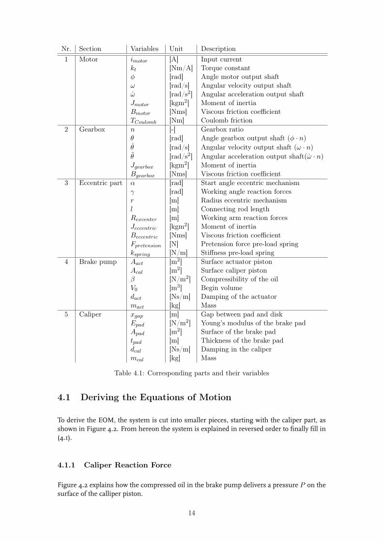
Nr. Section Variables Unit Description1 Motor imotor [A] Input current

kt [Nm/A] Torque constantφ [rad] Angle motor output shaftω [rad/s] Angular velocity output shaftω [rad/s2] Angular acceleration output shaftJmotor [kgm2] Moment of inertiaBmotor [Nms] Viscous friction coefficientTCoulomb [Nm] Coulomb friction

2 Gearbox n [-] Gearbox ratioθ [rad] Angle gearbox output shaft (φ · n)θ [rad/s] Angular velocity output shaft (ω · n)θ [rad/s2] Angular acceleration output shaft(ω · n)Jgearbox [kgm2] Moment of inertiaBgearbox [Nms] Viscous friction coefficient

3 Eccentric part α [rad] Start angle eccentric mechanismγ [rad] Working angle reaction forcesr [m] Radius eccentric mechanisml [m] Connecting rod lengthRexcenter [m] Working arm reaction forcesJeccentric [kgm2] Moment of inertiaBeccentric [Nms] Viscous friction coefficientFpretension [N] Pretension force pre-load springkspring [N/m] Stiffness pre-load spring

4 Brake pump Aact [m2] Surface actuator pistonAcal [m2] Surface caliper pistonβ [N/m2] Compressibility of the oilV0 [m3] Begin volumedact [Ns/m] Damping of the actuatormact [kg] Mass

5 Caliper xgap [m] Gap between pad and diskEpad [N/m2] Young’s modulus of the brake padApad [m2] Surface of the brake padtpad [m] Thickness of the brake paddcal [Ns/m] Damping in the calipermcal [kg] Mass

Table 4.1: Corresponding parts and their variables

4.1 Deriving the Equations of Motion

To derive the EOM, the system is cut into smaller pieces, starting with the caliper part, asshown in Figure 4.2. From hereon the system is explained in reversed order to finally fill in(4.1).

4.1.1 Caliper Reaction Force

Figure 4.2 explains how the compressed oil in the brake pump delivers a pressure P on thesurface of the calliper piston.

14

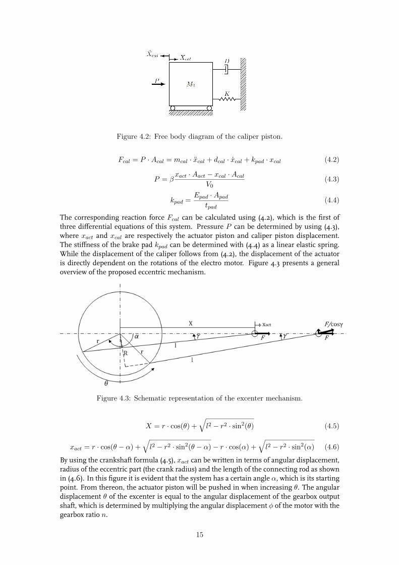
Figure 4.2: Free body diagram of the caliper piston.

Fcal = P ·Acal = mcal · xcal + dcal · xcal + kpad · xcal (4.2)

P = βxact ·Aact − xcal ·Acal

V0(4.3)

kpad =Epad ·Apad

tpad(4.4)

The corresponding reaction force Fcal can be calculated using (4.2), which is the first ofthree differential equations of this system. Pressure P can be determined by using (4.3),where xact and xcal are respectively the actuator piston and caliper piston displacement.The stiffness of the brake pad kpad can be determined with (4.4) as a linear elastic spring.While the displacement of the caliper follows from (4.2), the displacement of the actuatoris directly dependent on the rotations of the electro motor. Figure 4.3 presents a generaloverview of the proposed eccentric mechanism.

Figure 4.3: Schematic representation of the excenter mechanism.

X = r · cos(θ) +√l2 − r2 · sin2(θ) (4.5)

xact = r · cos(θ − α) +√l2 − r2 · sin2(θ − α)− r · cos(α) +

√l2 − r2 · sin2(α) (4.6)

By using the crankshaft formula (4.5), xact can be written in terms of angular displacement,radius of the eccentric part (the crank radius) and the length of the connecting rod as shownin (4.6). In this figure it is evident that the system has a certain angle α, which is its startingpoint. From thereon, the actuator piston will be pushed in when increasing θ. The angulardisplacement θ of the excenter is equal to the angular displacement of the gearbox outputshaft, which is determined by multiplying the angular displacement φ of the motor with thegearbox ratio n.

15

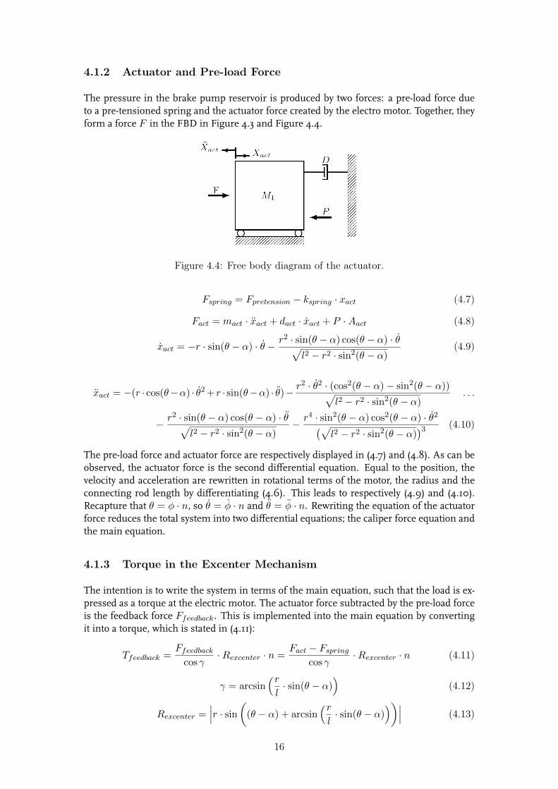
4.1.2 Actuator and Pre-load Force

The pressure in the brake pump reservoir is produced by two forces: a pre-load force dueto a pre-tensioned spring and the actuator force created by the electro motor. Together, theyform a force F in the FBD in Figure 4.3 and Figure 4.4.

Figure 4.4: Free body diagram of the actuator.

Fspring = Fpretension − kspring · xact (4.7)

Fact = mact · xact + dact · xact + P ·Aact (4.8)

xact = −r · sin(θ − α) · θ −r2 · sin(θ − α) cos(θ − α) · θ√

l2 − r2 · sin2(θ − α)(4.9)

xact = −(r · cos(θ−α) · θ2+ r · sin(θ−α) · θ)−r2 · θ2 · (cos2(θ − α)− sin2(θ − α))√

l2 − r2 · sin2(θ − α). . .

− r2 · sin(θ − α) cos(θ − α) · θ√l2 − r2 · sin2(θ − α)

− r4 · sin2(θ − α) cos2(θ − α) · θ2(√l2 − r2 · sin2(θ − α)

)3 (4.10)

The pre-load force and actuator force are respectively displayed in (4.7) and (4.8). As can beobserved, the actuator force is the second differential equation. Equal to the position, thevelocity and acceleration are rewritten in rotational terms of the motor, the radius and theconnecting rod length by differentiating (4.6). This leads to respectively (4.9) and (4.10).Recapture that θ = φ · n, so θ = φ · n and θ = φ · n. Rewriting the equation of the actuatorforce reduces the total system into two differential equations; the caliper force equation andthe main equation.

4.1.3 Torque in the Excenter Mechanism

The intention is to write the system in terms of the main equation, such that the load is ex-pressed as a torque at the electric motor. The actuator force subtracted by the pre-load forceis the feedback force Ffeedback. This is implemented into the main equation by convertingit into a torque, which is stated in (4.11):

Tfeedback =Ffeedbackcos γ

·Rexcenter · n =Fact − Fspring

cos γ·Rexcenter · n (4.11)

γ = arcsin(rl· sin(θ − α)

)(4.12)

Rexcenter =∣∣∣r · sin((θ − α) + arcsin

(rl· sin(θ − α)

))∣∣∣ (4.13)

16

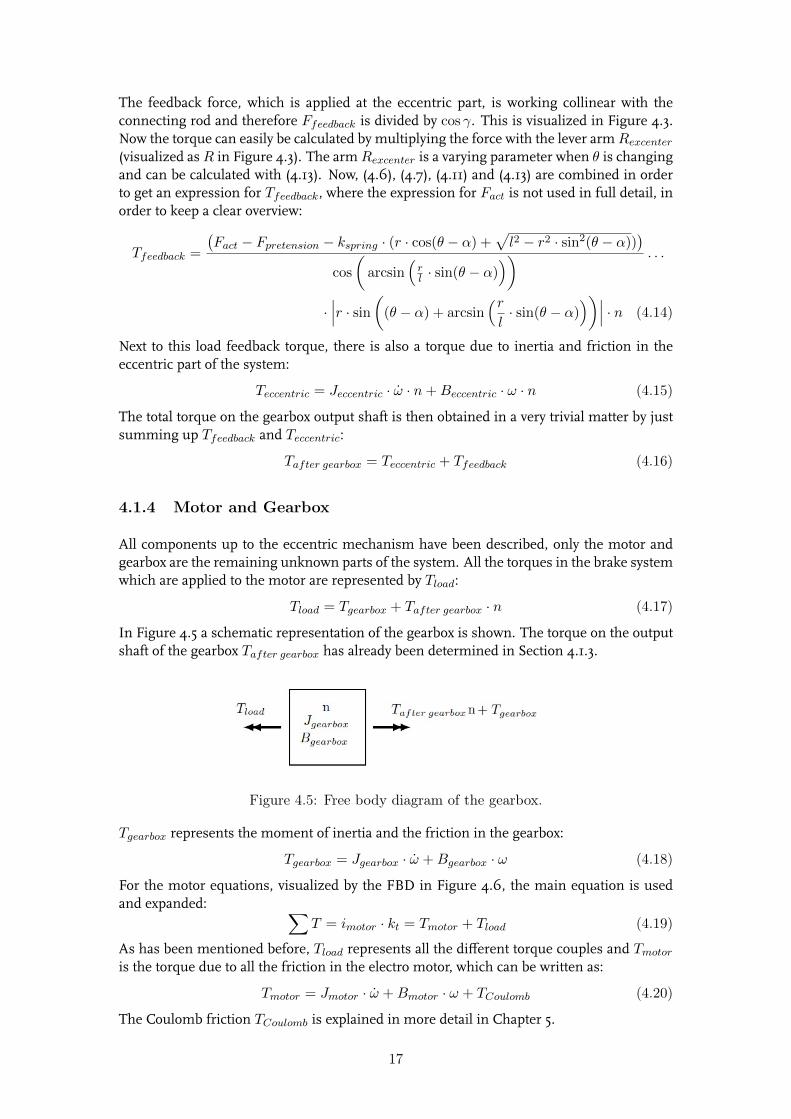
The feedback force, which is applied at the eccentric part, is working collinear with theconnecting rod and therefore Ffeedback is divided by cos γ. This is visualized in Figure 4.3.Now the torque can easily be calculated by multiplying the force with the lever armRexcenter(visualized asR in Figure 4.3). The armRexcenter is a varying parameter when θ is changingand can be calculated with (4.13). Now, (4.6), (4.7), (4.11) and (4.13) are combined in orderto get an expression for Tfeedback, where the expression for Fact is not used in full detail, inorder to keep a clear overview:

Tfeedback =

(Fact − Fpretension − kspring · (r · cos(θ − α) +

√l2 − r2 · sin2(θ − α))

)cos

(arcsin

(rl · sin(θ − α)

)) . . .

·∣∣∣r · sin((θ − α) + arcsin

(rl· sin(θ − α)

))∣∣∣ · n (4.14)

Next to this load feedback torque, there is also a torque due to inertia and friction in theeccentric part of the system:

Teccentric = Jeccentric · ω · n+Beccentric · ω · n (4.15)

The total torque on the gearbox output shaft is then obtained in a very trivial matter by justsumming up Tfeedback and Teccentric:

Tafter gearbox = Teccentric + Tfeedback (4.16)

4.1.4 Motor and Gearbox

All components up to the eccentric mechanism have been described, only the motor andgearbox are the remaining unknown parts of the system. All the torques in the brake systemwhich are applied to the motor are represented by Tload:

Tload = Tgearbox + Tafter gearbox · n (4.17)

In Figure 4.5 a schematic representation of the gearbox is shown. The torque on the outputshaft of the gearbox Tafter gearbox has already been determined in Section 4.1.3.

Figure 4.5: Free body diagram of the gearbox.

Tgearbox represents the moment of inertia and the friction in the gearbox:

Tgearbox = Jgearbox · ω +Bgearbox · ω (4.18)

For the motor equations, visualized by the FBD in Figure 4.6, the main equation is usedand expanded: ∑

T = imotor · kt = Tmotor + Tload (4.19)

As has been mentioned before, Tload represents all the different torque couples and Tmotoris the torque due to all the friction in the electro motor, which can be written as:

Tmotor = Jmotor · ω +Bmotor · ω + TCoulomb (4.20)

The Coulomb friction TCoulomb is explained in more detail in Chapter 5.

17

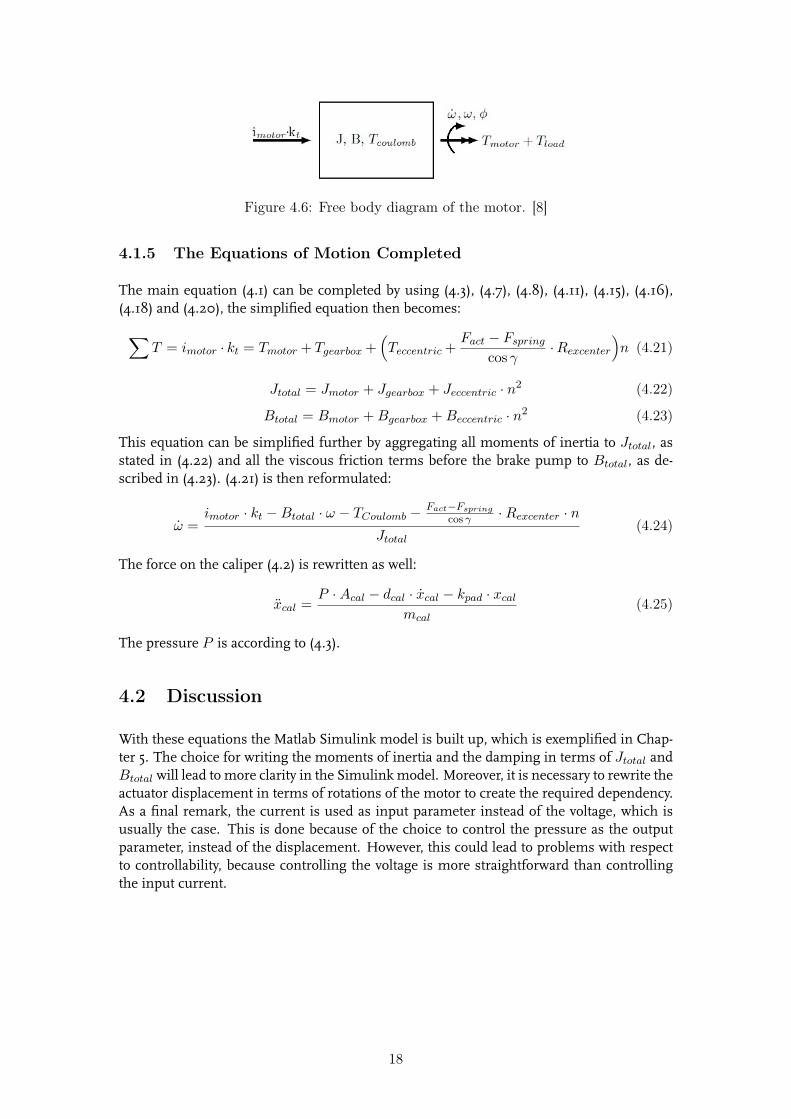
Figure 4.6: Free body diagram of the motor. [8]

4.1.5 The Equations of Motion Completed

The main equation (4.1) can be completed by using (4.3), (4.7), (4.8), (4.11), (4.15), (4.16),(4.18) and (4.20), the simplified equation then becomes:∑

T = imotor · kt = Tmotor + Tgearbox+(Teccentric+

Fact − Fspringcos γ

·Rexcenter)n (4.21)

Jtotal = Jmotor + Jgearbox + Jeccentric · n2 (4.22)

Btotal = Bmotor +Bgearbox +Beccentric · n2 (4.23)

This equation can be simplified further by aggregating all moments of inertia to Jtotal, asstated in (4.22) and all the viscous friction terms before the brake pump to Btotal, as de-scribed in (4.23). (4.21) is then reformulated:

ω =imotor · kt −Btotal · ω − TCoulomb −

Fact−Fspring

cos γ ·Rexcenter · nJtotal

(4.24)

The force on the caliper (4.2) is rewritten as well:

xcal =P ·Acal − dcal · xcal − kpad · xcal

mcal(4.25)

The pressure P is according to (4.3).

4.2 Discussion

With these equations the Matlab Simulink model is built up, which is exemplified in Chap-ter 5. The choice for writing the moments of inertia and the damping in terms of Jtotal andBtotal will lead to more clarity in the Simulink model. Moreover, it is necessary to rewrite theactuator displacement in terms of rotations of the motor to create the required dependency.As a final remark, the current is used as input parameter instead of the voltage, which isusually the case. This is done because of the choice to control the pressure as the outputparameter, instead of the displacement. However, this could lead to problems with respectto controllability, because controlling the voltage is more straightforward than controllingthe input current.

18

Chapter 5

Simulink Model of the DesignedBrake System

In this chapter, the Simulink model is described, that is used for analysing the brake system.First, the final EOM of Chapter 4 are used to create a Simulink model. Then the model issimplified, which will be explained in the corresponding section and finally, the Coulombfriction is clarified more extensively.

5.1 Equations of Motion in a Simulink Model

The Simulink model is set up using the EOM mentioned before. For clarity these equationsare repeated:

ω =i · kt −Btotal · ω − TCoulomb − Tfeedback · n

Jtotal(5.1)

Fact = mact · xact + dact · xact + P ·Aact (5.2)

xcal =P ·Acal − dcal · xcal − kpad · xcal

mcal(5.3)

First, the main equation is put into Simulink blocks. Using (5.1), the model depicted inFigure 5.1 is built. The system block called ’Coulomb Friction’ will be explained later inSection 5.3, because this type of friction is nontrivial. ’Tfeedback’ in this figure representsthe torque due to the reaction forces on the actuator side of the system. These reactionforces and corresponding displacements are put into Simulink blocks using the last partof this main equation and the equations of the actuator and caliper side, (5.2) and (5.3).The corresponding Simulink models can be seen in Figures 5.2 and 5.4. Because (5.2) isnot a stand alone differential equation and dependent on the rotational movement of themotor, the reaction force Fact is rewritten using (4.6), (4.9) and (4.10). The correspondingfunction block for the conversion of the translational terms into rotational terms is given inFigure 5.3. The Matlab codes inside the function blocks Torquefeedback and crank can befound in respectively Appendices A.1 and A.2. Finally, the pressure P needs to be definedas a combination of Simulink blocks. Recapture the pressure equation from Chapter 4:

P = βxact ·Aact − xcal ·Acal

V0(5.4)

This equation leads to Figure 5.5. The oil has compressibility β, which should be takeninto account because this will lead to different values of the stiffness for the whole system.

19

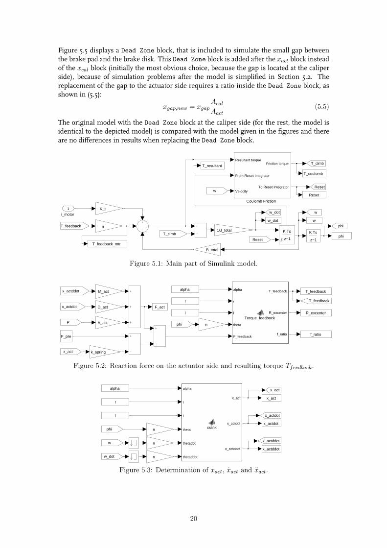
Figure 5.5 displays a Dead Zone block, that is included to simulate the small gap betweenthe brake pad and the brake disk. This Dead Zone block is added after the xact block insteadof the xcal block (initially the most obvious choice, because the gap is located at the caliperside), because of simulation problems after the model is simplified in Section 5.2. Thereplacement of the gap to the actuator side requires a ratio inside the Dead Zone block, asshown in (5.5):

xgap,new = xgapAcalAact

(5.5)

The original model with the Dead Zone block at the caliper side (for the rest, the model isidentical to the depicted model) is compared with the model given in the figures and thereare no differences in results when replacing the Dead Zone block.

w_dot w

phi

Reset

T_resultant

T_coulomb

T_feedback_mtr

phi

ww_dot

Reset

T_clmb

n

B_total

1/J_total

K_t

T_feedback

Reset

T_clmb

w

K Ts

z−1

K Ts

z−1

Coulomb Friction

Resultant torque

From Reset Integrator

Velocity

Friction torque

To Reset Integrator

i_motor1

Figure 5.1: Main part of Simulink model.

T_feedback

f_ratio

R_excenter

F_act

alpha

r

l

theta

F_feedback

T_feedback

R_excenter

f_ratio

Torque_feedback

T_feedback

A_act n

M_act

D_act

k_spring

x_actdot

phiP

x_act

x_actddot

r

alpha

l

F_pre

Figure 5.2: Reaction force on the actuator side and resulting torque Tfeedback.

x_actddot

x_actdot

x_act

alpha

r

l

theta

thetadot

thetaddot

x_act

x_actdot

x_actddot

crank

x_actddot

x_act

x_actdot

n

n

nw

w_dot

phi

r

alpha

l

Figure 5.3: Determination of xact, xact and xact.

20

x_cal_dotx_cal_ddot

x_cal1s

1s

x_calD_cal

1/M_cal

K_pad

A_calP

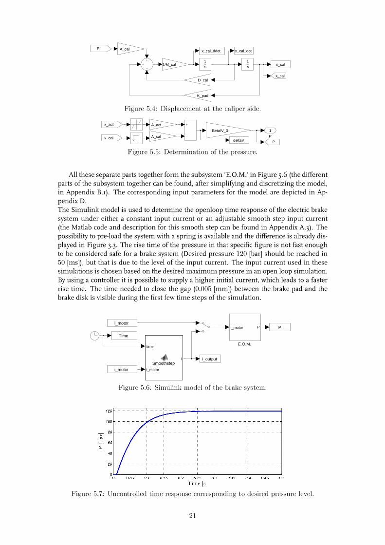
Figure 5.4: Displacement at the caliper side.

P1

deltaV P

A_act

Beta/V_0

A_cal

x_act

x_cal

Figure 5.5: Determination of the pressure.

All these separate parts together form the subsystem ’E.O.M.’ in Figure 5.6 (the differentparts of the subsystem together can be found, after simplifying and discretizing the model,in Appendix B.1). The corresponding input parameters for the model are depicted in Ap-pendix D.The Simulink model is used to determine the openloop time response of the electric brakesystem under either a constant input current or an adjustable smooth step input current(the Matlab code and description for this smooth step can be found in Appendix A.3). Thepossibility to pre-load the system with a spring is available and the difference is already dis-played in Figure 3.3. The rise time of the pressure in that specific figure is not fast enoughto be considered safe for a brake system (Desired pressure 120 [bar] should be reached in50 [ms]), but that is due to the level of the input current. The input current used in thesesimulations is chosen based on the desired maximum pressure in an open loop simulation.By using a controller it is possible to supply a higher initial current, which leads to a fasterrise time. The time needed to close the gap (0.005 [mm]) between the brake pad and thebrake disk is visible during the first few time steps of the simulation.

P

i_output

Time

time

i_motor

iSmoothstep

E.O.M.

i_motor P

i_motor

i_motor

Figure 5.6: Simulink model of the brake system.

Figure 5.7: Uncontrolled time response corresponding to desired pressure level.

21

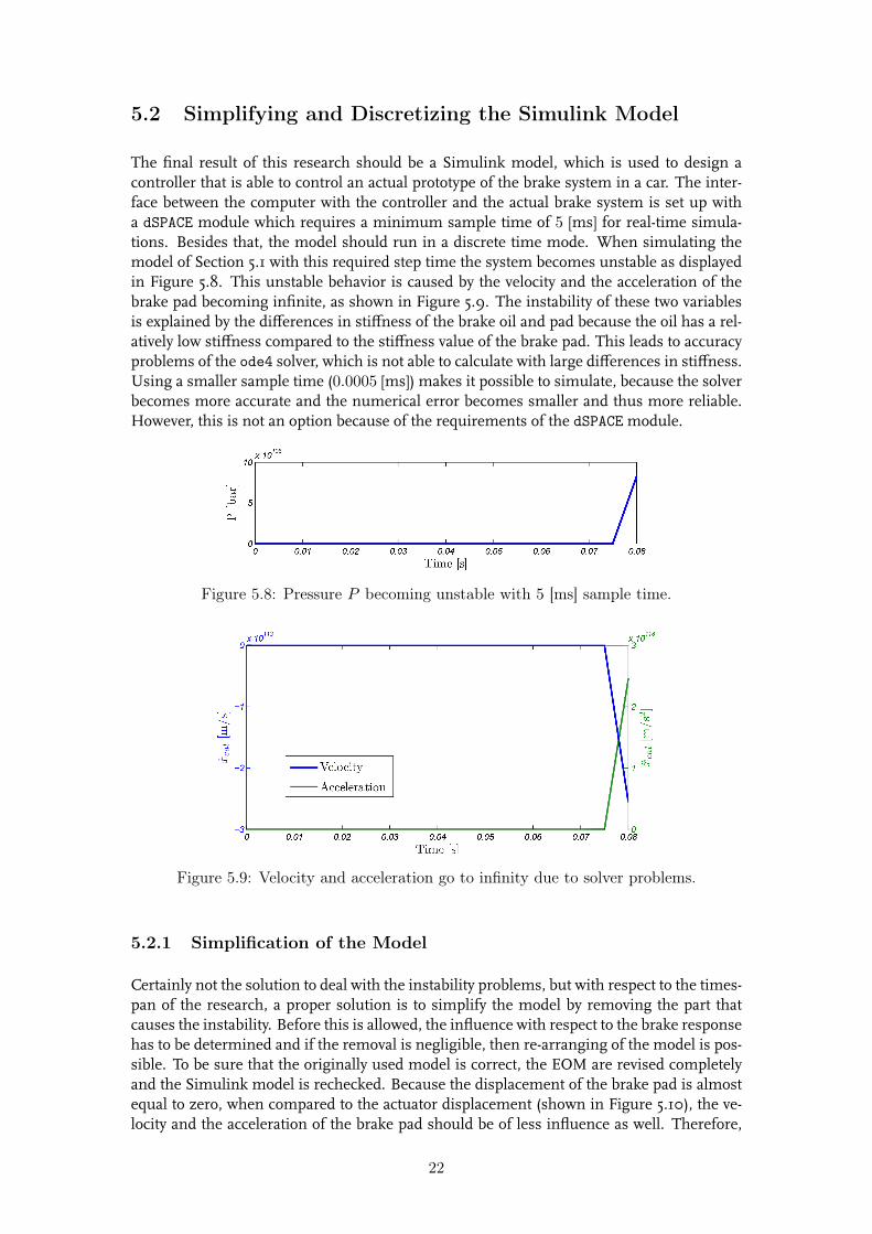
5.2 Simplifying and Discretizing the Simulink Model

The final result of this research should be a Simulink model, which is used to design acontroller that is able to control an actual prototype of the brake system in a car. The inter-face between the computer with the controller and the actual brake system is set up witha dSPACE module which requires a minimum sample time of 5 [ms] for real-time simula-tions. Besides that, the model should run in a discrete time mode. When simulating themodel of Section 5.1 with this required step time the system becomes unstable as displayedin Figure 5.8. This unstable behavior is caused by the velocity and the acceleration of thebrake pad becoming infinite, as shown in Figure 5.9. The instability of these two variablesis explained by the differences in stiffness of the brake oil and pad because the oil has a rel-atively low stiffness compared to the stiffness value of the brake pad. This leads to accuracyproblems of the ode4 solver, which is not able to calculate with large differences in stiffness.Using a smaller sample time (0.0005 [ms]) makes it possible to simulate, because the solverbecomes more accurate and the numerical error becomes smaller and thus more reliable.However, this is not an option because of the requirements of the dSPACE module.

Figure 5.8: Pressure P becoming unstable with 5 [ms] sample time.

Figure 5.9: Velocity and acceleration go to infinity due to solver problems.

5.2.1 Simplification of the Model

Certainly not the solution to deal with the instability problems, but with respect to the times-pan of the research, a proper solution is to simplify the model by removing the part thatcauses the instability. Before this is allowed, the influence with respect to the brake responsehas to be determined and if the removal is negligible, then re-arranging of the model is pos-sible. To be sure that the originally used model is correct, the EOM are revised completelyand the Simulink model is rechecked. Because the displacement of the brake pad is almostequal to zero, when compared to the actuator displacement (shown in Figure 5.10), the ve-locity and the acceleration of the brake pad should be of less influence as well. Therefore,

22

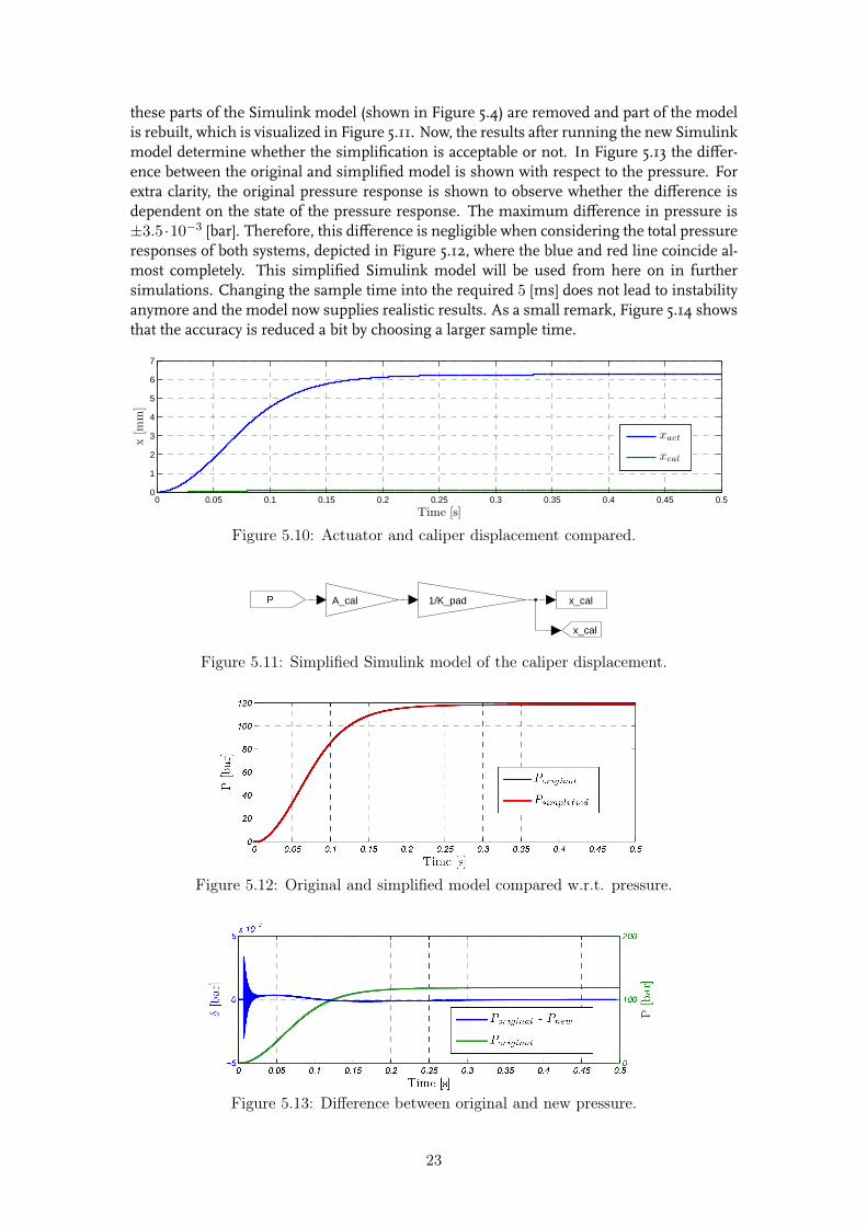
these parts of the Simulink model (shown in Figure 5.4) are removed and part of the modelis rebuilt, which is visualized in Figure 5.11. Now, the results after running the new Simulinkmodel determine whether the simplification is acceptable or not. In Figure 5.13 the differ-ence between the original and simplified model is shown with respect to the pressure. Forextra clarity, the original pressure response is shown to observe whether the difference isdependent on the state of the pressure response. The maximum difference in pressure is±3.5 ·10−3 [bar]. Therefore, this difference is negligible when considering the total pressureresponses of both systems, depicted in Figure 5.12, where the blue and red line coincide al-most completely. This simplified Simulink model will be used from here on in furthersimulations. Changing the sample time into the required 5 [ms] does not lead to instabilityanymore and the model now supplies realistic results. As a small remark, Figure 5.14 showsthat the accuracy is reduced a bit by choosing a larger sample time.

0 0.05 0.1 0.15 0.2 0.25 0.3 0.35 0.4 0.45 0.50

1

2

3

4

5

6

7

x[m

m]

Time [s]

xact

xcal

Figure 5.10: Actuator and caliper displacement compared.

x_cal

x_cal

A_cal 1/K_padP

Figure 5.11: Simplified Simulink model of the caliper displacement.

Figure 5.12: Original and simplified model compared w.r.t. pressure.

Figure 5.13: Difference between original and new pressure.

23

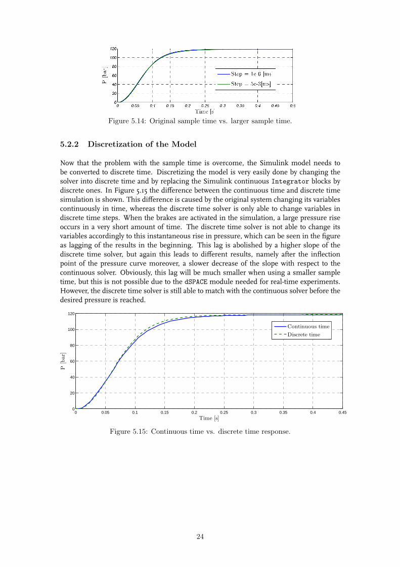
Figure 5.14: Original sample time vs. larger sample time.

5.2.2 Discretization of the Model

Now that the problem with the sample time is overcome, the Simulink model needs tobe converted to discrete time. Discretizing the model is very easily done by changing thesolver into discrete time and by replacing the Simulink continuous Integrator blocks bydiscrete ones. In Figure 5.15 the difference between the continuous time and discrete timesimulation is shown. This difference is caused by the original system changing its variablescontinuously in time, whereas the discrete time solver is only able to change variables indiscrete time steps. When the brakes are activated in the simulation, a large pressure riseoccurs in a very short amount of time. The discrete time solver is not able to change itsvariables accordingly to this instantaneous rise in pressure, which can be seen in the figureas lagging of the results in the beginning. This lag is abolished by a higher slope of thediscrete time solver, but again this leads to different results, namely after the inflectionpoint of the pressure curve moreover, a slower decrease of the slope with respect to thecontinuous solver. Obviously, this lag will be much smaller when using a smaller sampletime, but this is not possible due to the dSPACE module needed for real-time experiments.However, the discrete time solver is still able to match with the continuous solver before thedesired pressure is reached.

0 0.05 0.1 0.15 0.2 0.25 0.3 0.35 0.4 0.450

20

40

60

80

100

120

P[bar]

Time [s]

Continuous time

Discrete time

Figure 5.15: Continuous time vs. discrete time response.

24

5.3 Coulomb Friction of the Motor

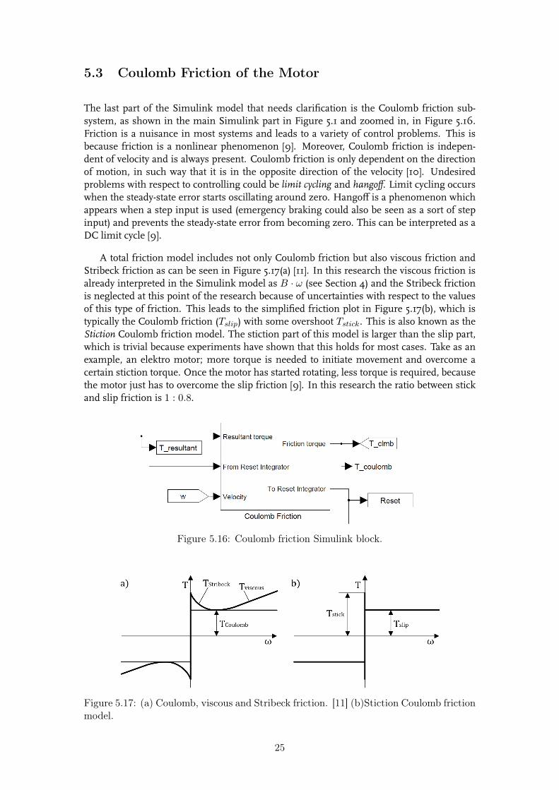
The last part of the Simulink model that needs clarification is the Coulomb friction sub-system, as shown in the main Simulink part in Figure 5.1 and zoomed in, in Figure 5.16.Friction is a nuisance in most systems and leads to a variety of control problems. This isbecause friction is a nonlinear phenomenon [9]. Moreover, Coulomb friction is indepen-dent of velocity and is always present. Coulomb friction is only dependent on the directionof motion, in such way that it is in the opposite direction of the velocity [10]. Undesiredproblems with respect to controlling could be limit cycling and hangoff. Limit cycling occurswhen the steady-state error starts oscillating around zero. Hangoff is a phenomenon whichappears when a step input is used (emergency braking could also be seen as a sort of stepinput) and prevents the steady-state error from becoming zero. This can be interpreted as aDC limit cycle [9].

A total friction model includes not only Coulomb friction but also viscous friction andStribeck friction as can be seen in Figure 5.17(a) [11]. In this research the viscous friction isalready interpreted in the Simulink model as B · ω (see Section 4) and the Stribeck frictionis neglected at this point of the research because of uncertainties with respect to the valuesof this type of friction. This leads to the simplified friction plot in Figure 5.17(b), which istypically the Coulomb friction (Tslip) with some overshoot Tstick. This is also known as theStiction Coulomb friction model. The stiction part of this model is larger than the slip part,which is trivial because experiments have shown that this holds for most cases. Take as anexample, an elektro motor; more torque is needed to initiate movement and overcome acertain stiction torque. Once the motor has started rotating, less torque is required, becausethe motor just has to overcome the slip friction [9]. In this research the ratio between stickand slip friction is 1 : 0.8.

Figure 5.16: Coulomb friction Simulink block.

Figure 5.17: (a) Coulomb, viscous and Stribeck friction. [11] (b)Stiction Coulomb frictionmodel.

25

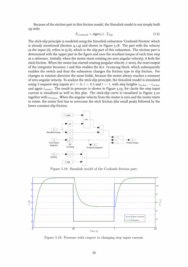
Because of the stiction part in this friction model, the Simulink model is not simply builtup with:

TCoulomb = sign(ω) · Tslip (5.6)

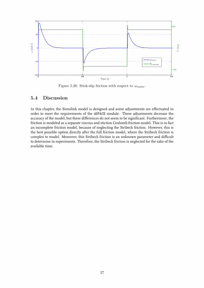
The stick-slip principle is modeled using the Simulink subsystem ’Coulomb Friction’ whichis already mentioned (Section 4.1.4) and shown in Figure 5.18. The part with the velocityas the input (3), refers to (5.6), which is the slip part of this subsystem. The stiction part isdetermined with the upper part in the figure and uses the resultant torque of each time stepas a reference. Initially, when the motor starts rotating (so zero angular velocity), it feels thestick friction. When the motor has started rotating (angular velocity 6= zero), the reset outputof the integrator becomes 1 and this enables the Hit Crossing block, which subsequentlyenables the switch and thus the subsystem changes the friction type to slip friction. Forchanges in rotation direction the same holds, because the motor always reaches a momentof zero angular velocity. To analyse the stick-slip principle, the Simulink model is simulatedusing 3 sequent step inputs at t = 0, t = 0.5 and t = 1, with step heights imotor, −imotorand again imotor. The result in pressure is shown in Figure 5.19, for clarity the step inputcurrent is visualized as well in this plot. The stick-slip curve is visualized in Figure 5.20together with ωmotor. When the angular velocity from the motor is zero and the motor startsto rotate, the motor first has to overcome the stick friction (the small peak) followed by thelower constant slip friction.

To Reset Integrator

2Friction torque

1 >

min

Hit Crossing

T_slip

T_stick

|u|

Velocity3

From ResetIntegrator

2

Resultant torque1

Figure 5.18: Simulink model of the Coulomb friction part.

0 0.5 1 1.5

0

1

2

3

4

5

6

I[A

]

Time [s]

0 0.5 1 1.50

20

40

60

80

100

120

P[bar]

Input current

Pressure

Figure 5.19: Pressure with respect to changing step input current.

26

0 0.5 1 1.5−100

−50

0

50

100

ω[rad/s]

Time [s]

0 0.5 1 1.5

−0.02

0

0.02

T[N

m]

ωmotor

TCoulomb

Figure 5.20: Stick-slip friction with respect to ωmotor.

5.4 Discussion

In this chapter, the Simulink model is designed and some adjustments are effectuated inorder to meet the requirements of the dSPACE module. These adjustments decrease theaccuracy of the model, but these differences do not seem to be significant. Furthermore, thefriction is modeled as a separate viscous and stiction Coulomb friction model. This is in factan incomplete friction model, because of neglecting the Stribeck friction. However, this isthe best possible option directly after the full friction model, where the Stribeck friction iscomplex to model. Moreover, this Stribeck friction is an unknown parameter and difficultto determine in experiments. Therefore, the Stribeck friction is neglected for the sake of theavailable time.

27

28

Chapter 6

Controller Design for the BrakeSystem

Now that the Simulink model has been derived in Chapter 5, a controller has to be designedsuch that a desired input pressure from the ECU yields an appropriate signal for the electromotor of the brake system. The brake pressure, which is the output of the brake system,may never contain overshoot, must be as smooth and as fast as possible and be robust tovarying system parameters.In order to get this desired behavior, two types of controllers are designed to develop anoptimal controller, which features the best possible performance and robustness. First, aproportional-integral-derivative controller is considered for its implementation ease, tuningand performance. The second controller is a sliding mode controller, which has excellentperformance for nonlinear systems and a tuneable robustness against uncertainties. Feedforward control is not considered due to its limitations in regard to system parameters anddisturbances, these could vary over time and thus affect the controller performance nega-tively.

6.1 PID Controller

The standard representation of PID control in the time domain is given by

u(t) = Kpe(t) +Kdde(t)

dt+Ki

∫e(t)dt (6.1)

Where u is the controller output, Kp, Kd (Kd = Kpτd) and Ki (Ki =Kp

τi) respectively

the proportional, derivative and integral gains and e(t) the error. This error consists of thereference signal r(t) minus the proces signal y(t). This time domain representation can berewritten into the discrete time domain by using the Forward Euler approximation for boththe integrator and filter method. The Simulink representation of the discrete time form isgiven by

u(t) = Kp +KiTsz − 1

+KdN

1 + N ·Tsz−1

(6.2)

where Ts is the discrete sampling time, N the filter coefficient, z the current time stepand Kp, Ki and Kd the PID gains. Each of the coefficients of the proportional, integral andderivative gains have influence on the characteristics of the system response. They have tobe tuned accurately in order to get the desired performance.

29

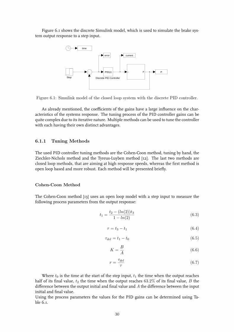
Figure 6.1 shows the discrete Simulink model, which is used to simulate the brake sys-tem output response to a step input.

P

error current

time

i P

Step Discrete PID Controller

PID(z)

Figure 6.1: Simulink model of the closed loop system with the discrete PID controller.

As already mentioned, the coefficients of the gains have a large influence on the char-acteristics of the systems response. The tuning process of the PID controller gains can bequite complex due to its iterative nature. Multiple methods can be used to tune the controllerwith each having their own distinct advantages.

6.1.1 Tuning Methods

The used PID controller tuning methods are the Cohen-Coon method, tuning by hand, theZiechler-Nichols method and the Tyreus-Luyben method [12]. The last two methods areclosed loop methods, that are aiming at high response speeds, whereas the first method isopen loop based and more robust. Each method will be presented briefly.

Cohen-Coon Method

The Cohen-Coon method [13] uses an open loop model with a step input to measure thefollowing process parameters from the output response:

t1 =t2 − (ln(2))t31− ln(2)

(6.3)

τ = t3 − t1 (6.4)

τdel = t1 − t0 (6.5)

K =B

A(6.6)

r =τdelτ

(6.7)

Where t0 is the time at the start of the step input, t1 the time when the output reacheshalf of its final value, t2 the time when the output reaches 63.2% of its final value, B thedifference between the output initial and final value and A the difference between the inputinitial and final value.Using the process parameters the values for the PID gains can be determined using Ta-ble 6.1.

30

Kp Ki Kd

tuning rules 1rK

(43 + r

4

)τdel

32+6r13+8r τdel

411+2r

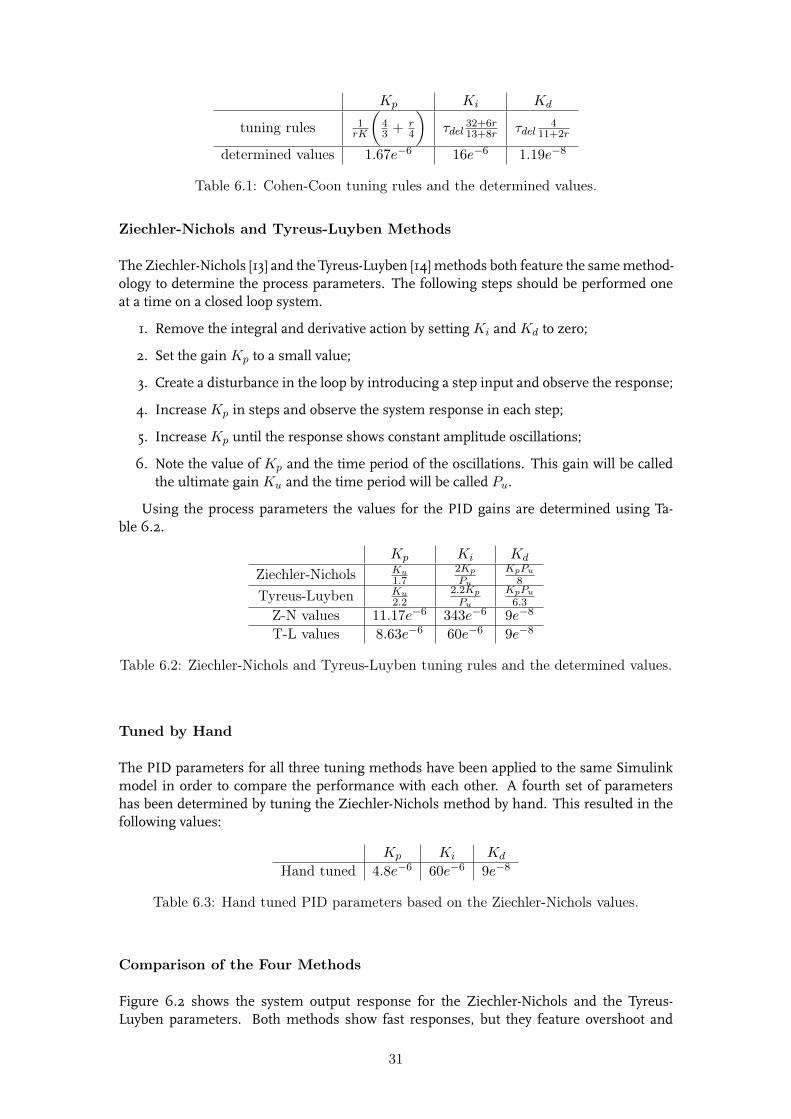
determined values 1.67e−6 16e−6 1.19e−8

Table 6.1: Cohen-Coon tuning rules and the determined values.

Ziechler-Nichols and Tyreus-Luyben Methods

The Ziechler-Nichols [13] and the Tyreus-Luyben [14] methods both feature the same method-ology to determine the process parameters. The following steps should be performed oneat a time on a closed loop system.

1. Remove the integral and derivative action by setting Ki and Kd to zero;

2. Set the gain Kp to a small value;

3. Create a disturbance in the loop by introducing a step input and observe the response;

4. Increase Kp in steps and observe the system response in each step;

5. Increase Kp until the response shows constant amplitude oscillations;

6. Note the value of Kp and the time period of the oscillations. This gain will be calledthe ultimate gain Ku and the time period will be called Pu.

Using the process parameters the values for the PID gains are determined using Ta-ble 6.2.

Kp Ki Kd

Ziechler-Nichols Ku1.7

2Kp

Pu

KpPu

8

Tyreus-Luyben Ku2.2

2.2Kp

Pu

KpPu

6.3

Z-N values 11.17e−6 343e−6 9e−8

T-L values 8.63e−6 60e−6 9e−8

Table 6.2: Ziechler-Nichols and Tyreus-Luyben tuning rules and the determined values.

Tuned by Hand

The PID parameters for all three tuning methods have been applied to the same Simulinkmodel in order to compare the performance with each other. A fourth set of parametershas been determined by tuning the Ziechler-Nichols method by hand. This resulted in thefollowing values:

Kp Ki Kd

Hand tuned 4.8e−6 60e−6 9e−8

Table 6.3: Hand tuned PID parameters based on the Ziechler-Nichols values.

Comparison of the Four Methods

Figure 6.2 shows the system output response for the Ziechler-Nichols and the Tyreus-Luyben parameters. Both methods show fast responses, but they feature overshoot and

31

some oscillations as well, while the Cohen-Coon parameters lead to a slower response butno oscillations. The hand tuned values, which were based on the Ziechler-Nichols parame-ters, show a slightly slower response than the first two but without any overshoot.

0 0.05 0.1 0.15 0.2 0.25 0.3 0.35 0.4 0.45 0.50

20

40

60

80

100

120

140

160

P[bar]

Time [s]

Cohen-Coon

Ziechler-Nichols

Tyreus-Luyben

Hand tuned

Figure 6.2: Closed loop output pressure responses to a step input of 100 [bar] with PIDgain values according to the different tuning methods.

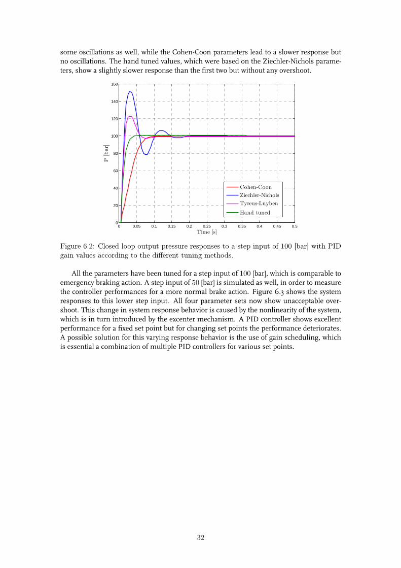
All the parameters have been tuned for a step input of 100 [bar], which is comparable toemergency braking action. A step input of 50 [bar] is simulated as well, in order to measurethe controller performances for a more normal brake action. Figure 6.3 shows the systemresponses to this lower step input. All four parameter sets now show unacceptable over-shoot. This change in system response behavior is caused by the nonlinearity of the system,which is in turn introduced by the excenter mechanism. A PID controller shows excellentperformance for a fixed set point but for changing set points the performance deteriorates.A possible solution for this varying response behavior is the use of gain scheduling, whichis essential a combination of multiple PID controllers for various set points.

32

0 0.05 0.1 0.15 0.2 0.25 0.3 0.35 0.4 0.45 0.50

10

20

30

40

50

60

70

80

90

P[bar]

Time [s]

Cohen-Coon

Ziechler-Nichols

Tyreus-Luyben

Hand tuned

Figure 6.3: Closed loop output pressure responses to a step input of 50 [bar] with PIDgain values according to the different tuning methods.

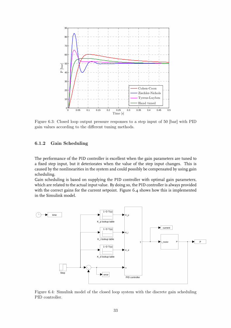
6.1.2 Gain Scheduling

The performance of the PID controller is excellent when the gain parameters are tuned toa fixed step input, but it deteriorates when the value of the step input changes. This iscaused by the nonlinearities in the system and could possibly be compensated by using gainscheduling.Gain scheduling is based on supplying the PID controller with optimal gain parameters,which are related to the actual input value. By doing so, the PID controller is always providedwith the correct gains for the current setpoint. Figure 6.4 shows how this is implementedin the Simulink model.

P

error

current

time

i_motor P

Step

PID controller

K_p

K_i

K_d

u

y

K_p lookup table

1−D T(u)

K_i lookup table

1−D T(u)

K_d lookup table

1−D T(u)

Figure 6.4: Simulink model of the closed loop system with the discrete gain schedulingPID controller.

33

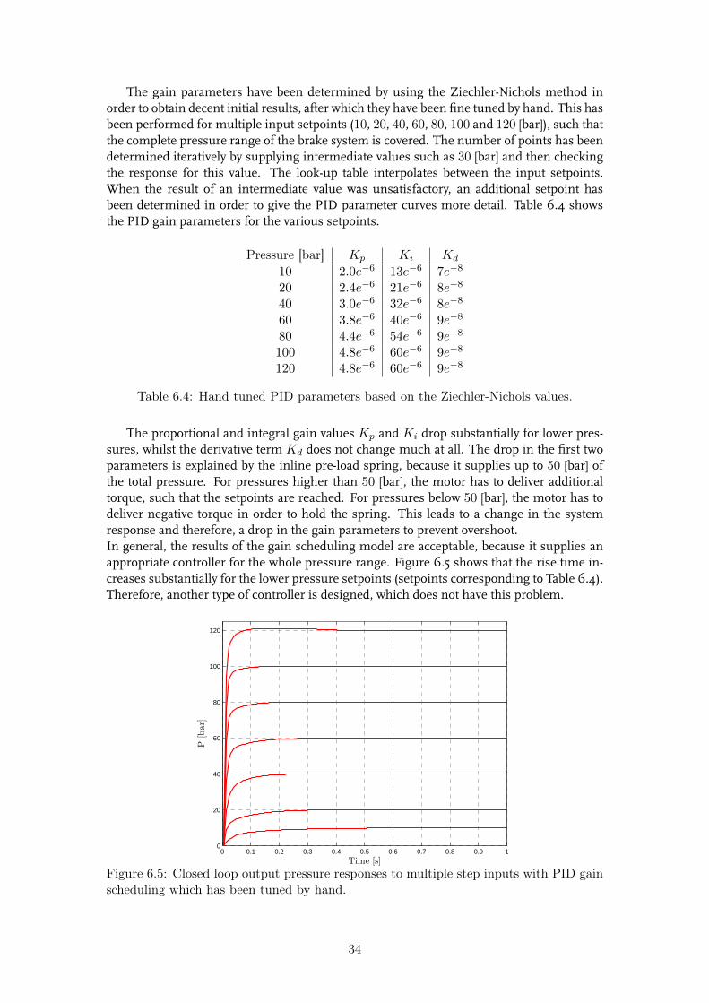
The gain parameters have been determined by using the Ziechler-Nichols method inorder to obtain decent initial results, after which they have been fine tuned by hand. This hasbeen performed for multiple input setpoints (10, 20, 40, 60, 80, 100 and 120 [bar]), such thatthe complete pressure range of the brake system is covered. The number of points has beendetermined iteratively by supplying intermediate values such as 30 [bar] and then checkingthe response for this value. The look-up table interpolates between the input setpoints.When the result of an intermediate value was unsatisfactory, an additional setpoint hasbeen determined in order to give the PID parameter curves more detail. Table 6.4 showsthe PID gain parameters for the various setpoints.

Pressure [bar] Kp Ki Kd

10 2.0e−6 13e−6 7e−8

20 2.4e−6 21e−6 8e−8

40 3.0e−6 32e−6 8e−8

60 3.8e−6 40e−6 9e−8

80 4.4e−6 54e−6 9e−8

100 4.8e−6 60e−6 9e−8

120 4.8e−6 60e−6 9e−8

Table 6.4: Hand tuned PID parameters based on the Ziechler-Nichols values.

The proportional and integral gain values Kp and Ki drop substantially for lower pres-sures, whilst the derivative term Kd does not change much at all. The drop in the first twoparameters is explained by the inline pre-load spring, because it supplies up to 50 [bar] ofthe total pressure. For pressures higher than 50 [bar], the motor has to deliver additionaltorque, such that the setpoints are reached. For pressures below 50 [bar], the motor has todeliver negative torque in order to hold the spring. This leads to a change in the systemresponse and therefore, a drop in the gain parameters to prevent overshoot.In general, the results of the gain scheduling model are acceptable, because it supplies anappropriate controller for the whole pressure range. Figure 6.5 shows that the rise time in-creases substantially for the lower pressure setpoints (setpoints corresponding to Table 6.4).Therefore, another type of controller is designed, which does not have this problem.

0 0.1 0.2 0.3 0.4 0.5 0.6 0.7 0.8 0.9 10

20

40

60

80

100

120

P[bar]

Time [s]

Figure 6.5: Closed loop output pressure responses to multiple step inputs with PID gainscheduling which has been tuned by hand.

34

6.2 Sliding Mode Controller

Sliding Mode Control is a Lyapunov based control method and it is a populair strategie todeal with uncertain systems [15], such as the proposed brake system. A sliding mode con-troller is a variable structure controller, that alters the dynamics of the nonlinear system byapplication of a high frequency switching control. The feedback contains several continuousfunctions from which is being switched by the switching function.

In order to be sure that the sliding mode starts at a certain time t > 0, independent ofthe initial state x(0), the following η -reachability condition should meet

ss ≤ −η|s| (6.8)

where s is the sliding surface. This is rewritten into a constant + proportional rate, reachinglaw approach, which expresses the dynamics of the sliding function directly:

s = −k · s− η · sign(s) (6.9)

Here, k and η are positive, constant parameters and s is the continous time, switchingfunction. Before the sliding surface can be introduced, first the pressure error is introduced:

e(k) = Pd(k)− P (k) (6.10)

Where Pd and P are the respective responses of the desired reference pressure and theactual pressure at the kth sampling interval. Now, the sliding surface (s) can be defined:

s = e+ λ1

∫edt+ λ2e (6.11)

Herein is e the rate of change of e, e the pressure error,∫edt the integral of the pressure

error and λ1 and λ2 positive real constants.

In order to rewrite (6.9) to the control signal, the derivative of (6.11) is needed:

s = e+ λ1e+ λ2e (6.12)

Usinge = Pd − P (6.13)

e = Pd − P (6.14)

and

P = βxact ·Aact − xcal ·Acal

V0(6.15)

P = βxact ·Aact

V0(6.16)

P = βxact ·Aact

V0(6.17)

where xact, xact and xact are as in (4.6), (4.9) and (4.10). An expression for θ, only depen-dent on the variables i, θ and θ, can be determined by rewriting (4.21) into:

θ = i · kt − . . . (6.18)

35

The full expression for (6.18) can be found in Appendix (C.1). This expression is insertedinto xact of (6.17), such that θ is cancelled and i is introduced (The exact derivation is shownin Appendix C). Equation (6.9) can now be rewritten into the following form:

P =

((k+λ1) ·(Pd−P )+kλ1 ·

∫(Pd−P )+(kλ2+1) ·(Pd− P )+η ·sign

[(Pd−P ) . . .

+

∫(Pd − P ) + (Pd − P )

])· λ2 + Pd (6.19)

Where P contains θ, θ and i in order to introduce the control signal into the equation ofthe sliding mode controller. Equation (6.19) shows that the following input parameters arenecessary for the sliding mode controller to operate properly:

• Pd : The desired pressure;

• Pd : The desired pressure rate;

• Pd : The desired pressure change of rate;

• P : The actual system pressure;

• φ : the motor rotation;

• ω : the motor speed.

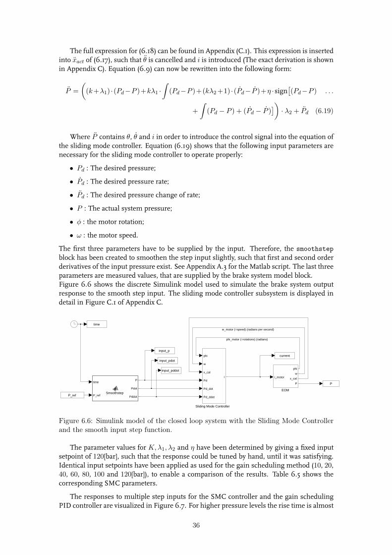
The first three parameters have to be supplied by the input. Therefore, the smoothstepblock has been created to smoothen the step input slightly, such that first and second orderderivatives of the input pressure exist. See Appendix A.3 for the Matlab script. The last threeparameters are measured values, that are supplied by the brake system model block.Figure 6.6 shows the discrete Simulink model used to simulate the brake system outputresponse to the smooth step input. The sliding mode controller subsystem is displayed indetail in Figure C.1 of Appendix C.

P

input_pddot

input_pdot

input_p

current

time

Sliding Mode Controller

phi

w

x_cal

Pd

Pd_dot

Pd_ddot

i

time

P_ref

P

Pdot

PddotSmoothstep

EOM

i_motor

phi

w

x_cal

P

P_ref

phi_motor (=rotations) (radians)

w_motor (=speed) (radians per second)

Figure 6.6: Simulink model of the closed loop system with the Sliding Mode Controllerand the smooth input step function.

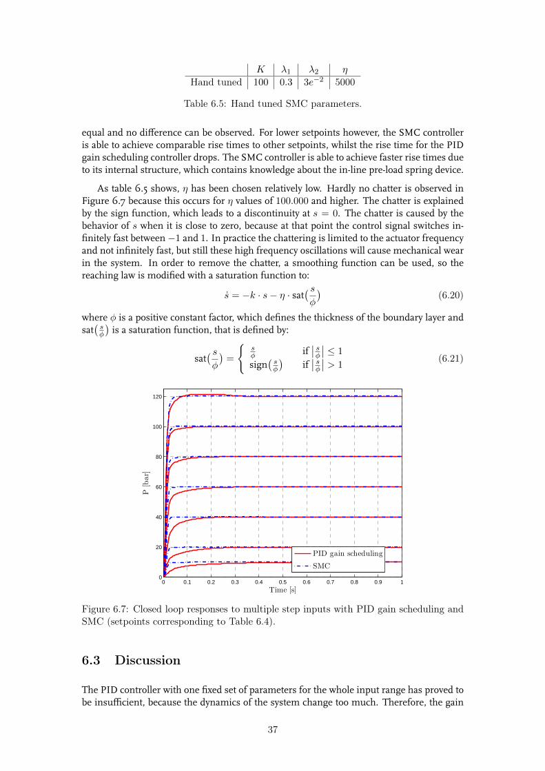
The parameter values for K,λ1, λ2 and η have been determined by giving a fixed inputsetpoint of 120[bar], such that the response could be tuned by hand, until it was satisfying.Identical input setpoints have been applied as used for the gain scheduling method (10, 20,40, 60, 80, 100 and 120[bar]), to enable a comparison of the results. Table 6.5 shows thecorresponding SMC parameters.

The responses to multiple step inputs for the SMC controller and the gain schedulingPID controller are visualized in Figure 6.7. For higher pressure levels the rise time is almost

36

K λ1 λ2 η

Hand tuned 100 0.3 3e−2 5000

Table 6.5: Hand tuned SMC parameters.

equal and no difference can be observed. For lower setpoints however, the SMC controlleris able to achieve comparable rise times to other setpoints, whilst the rise time for the PIDgain scheduling controller drops. The SMC controller is able to achieve faster rise times dueto its internal structure, which contains knowledge about the in-line pre-load spring device.

As table 6.5 shows, η has been chosen relatively low. Hardly no chatter is observed inFigure 6.7 because this occurs for η values of 100.000 and higher. The chatter is explainedby the sign function, which leads to a discontinuity at s = 0. The chatter is caused by thebehavior of s when it is close to zero, because at that point the control signal switches in-finitely fast between−1 and 1. In practice the chattering is limited to the actuator frequencyand not infinitely fast, but still these high frequency oscillations will cause mechanical wearin the system. In order to remove the chatter, a smoothing function can be used, so thereaching law is modified with a saturation function to:

s = −k · s− η · sat( sφ

)(6.20)

where φ is a positive constant factor, which defines the thickness of the boundary layer andsat(sφ

)is a saturation function, that is defined by:

sat( sφ

)=

{sφ if

∣∣ sφ

∣∣ ≤ 1

sign(sφ

)if∣∣ sφ

∣∣ > 1(6.21)

0 0.1 0.2 0.3 0.4 0.5 0.6 0.7 0.8 0.9 10

20

40

60

80

100

120

P[bar]

Time [s]

PID gain scheduling

SMC

Figure 6.7: Closed loop responses to multiple step inputs with PID gain scheduling andSMC (setpoints corresponding to Table 6.4).

6.3 Discussion

The PID controller with one fixed set of parameters for the whole input range has proved tobe insufficient, because the dynamics of the system change too much. Therefore, the gain

37

scheduling method was introduced. This method resulted in a smooth response withoutany overshoot, although for low pressures the rise time became larger due to the pre-loadspring mechanism. In order to solve this problem as well, a SMC controller, capable ofachieving smooth responses with equal rise times at any setpoint, has been designed.

38

Chapter 7

Experimental Setup and Results

7.1 Experimental Setup

This section discusses the component selection and the 3D CAD model of the prototype,followed by detailed information on each component of the measurement setup used todetermine the performance of the actual system.

7.1.1 Preliminary Experiment

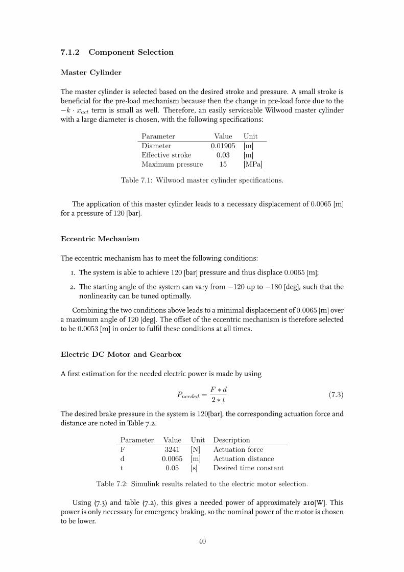
An experiment is performed prior to the design of the prototype, in order to determinewhether the simulation results correspond to the real system, such that the prototype canbe designed accurately. A simple measurement has been performed in the lab on a brakecaliper of the Equinox brake system to determine the volume displacement needed to achieve120 [bar] pressure. By using a ball screw actuated piston (d=14.2 [mm]) the displacementwas accurately measured to be 12 [mm]. This leads to the following displacement volume:

Vmeasured = 0.012 ∗ π4∗ 0.01422 = 1.90e−6 (7.1)

Using the same actuator piston diameter in the simulation, this leads to a piston dis-placement of ≈ 1[mm]:

Vsimulation = 0.001 ∗ π4∗ 0.01422 = 1.58e−7 (7.2)

This implies that there is a difference of factor 1.9e−6

1.58e−7 = 12 between the stiffness of themeasurements and simulations.In order to compensate for this discrepancy, the bulk modulus β and the pad stiffness Kpad haveboth been lowered by a factor 10 to drop the total stiffness of the system by an equal amount.By doing so the displacement of the simulation is more in accordance with the real system,such that the components can be selected accurately. The reason(s) for the large deviationbetween the two values will be discussed in Chapter 8.

39

7.1.2 Component Selection

Master Cylinder

The master cylinder is selected based on the desired stroke and pressure. A small stroke isbeneficial for the pre-load mechanism because then the change in pre-load force due to the−k · xact term is small as well. Therefore, an easily serviceable Wilwood master cylinderwith a large diameter is chosen, with the following specifications:

Parameter Value UnitDiameter 0.01905 [m]Effective stroke 0.03 [m]Maximum pressure 15 [MPa]

Table 7.1: Wilwood master cylinder specifications.

The application of this master cylinder leads to a necessary displacement of 0.0065 [m]for a pressure of 120 [bar].

Eccentric Mechanism

The eccentric mechanism has to meet the following conditions:

1. The system is able to achieve 120 [bar] pressure and thus displace 0.0065 [m];

2. The starting angle of the system can vary from −120 up to −180 [deg], such that thenonlinearity can be tuned optimally.

Combining the two conditions above leads to a minimal displacement of 0.0065 [m] overa maximum angle of 120 [deg]. The offset of the eccentric mechanism is therefore selectedto be 0.0053 [m] in order to fulfil these conditions at all times.

Electric DC Motor and Gearbox

A first estimation for the needed electric power is made by using

Pneeded =F ∗ d2 ∗ t

(7.3)

The desired brake pressure in the system is 120[bar], the corresponding actuation force anddistance are noted in Table 7.2.

Parameter Value Unit DescriptionF 3241 [N] Actuation forced 0.0065 [m] Actuation distancet 0.05 [s] Desired time constant

Table 7.2: Simulink results related to the electric motor selection.

Using (7.3) and table (7.2), this gives a needed power of approximately 210[W]. Thispower is only necessary for emergency braking, so the nominal power of the motor is chosento be lower.

40

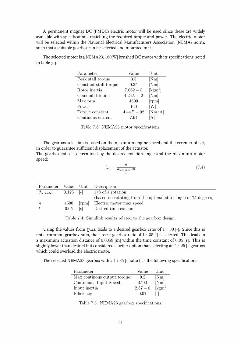
A permanent magnet DC (PMDC) electric motor will be used since these are widelyavailable with specifications matching the required torque and power. The electric motorwill be selected within the National Electrical Manufacturers Association (NEMA) norm,such that a suitable gearbox can be selected and mounted to it.

The selected motor is a NEMA23, 160[W] brushed DC motor with its specifications notedin table 7.3.

Parameter Value UnitPeak stall torque 3.5 [Nm]Constant stall torque 0.35 [Nm]Rotor inertia 7.062− 5 [kgm2]Coulomb friction 4.24E − 2 [Nm]Max prm 4500 [rpm]Power 160 [W]Torque constant 4.44E − 02 [Nm/A]Continous current 7.94 [A]

Table 7.3: NEMA23 motor specifications.

The gearbox selection is based on the maximum engine speed and the eccenter offset,in order to guarantee sufficient displacement of the actuator.The gearbox ratio is determined by the desired rotation angle and the maximum motorspeed:

igb =n

θeccenter·60t

(7.4)

Parameter Value Unit Descriptionθeccenter 0.125 [-] 1/8 of a rotation

(based on rotating from the optimal start angle of 75 degrees)n 4500 [rpm] Electric motor max speedt 0.05 [s] Desired time constant

Table 7.4: Simulink results related to the gearbox design.

Using the values from (7.4), leads to a desired gearbox ratio of 1 : 30 [-]. Since this isnot a common gearbox ratio, the closest gearbox ratio of 1 : 35 [-] is selected. This leads toa maximum actuation distance of 0.0059 [m] within the time constant of 0.05 [s]. This isslightly lower than desired but considered a better option than selecting an 1 : 25 [-] gearboxwhich could overload the electric motor.

The selected NEMA23 gearbox with a 1 : 35 [-] ratio has the following specifications :

Parameter Value UnitMax continous output torque 9.2 [Nm]Continuous Input Speed 4500 [Nm]Input inertia 2.57− 8 [kgm2]Efficiency 0.97 [-]

Table 7.5: NEMA23 gearbox specifications.

41

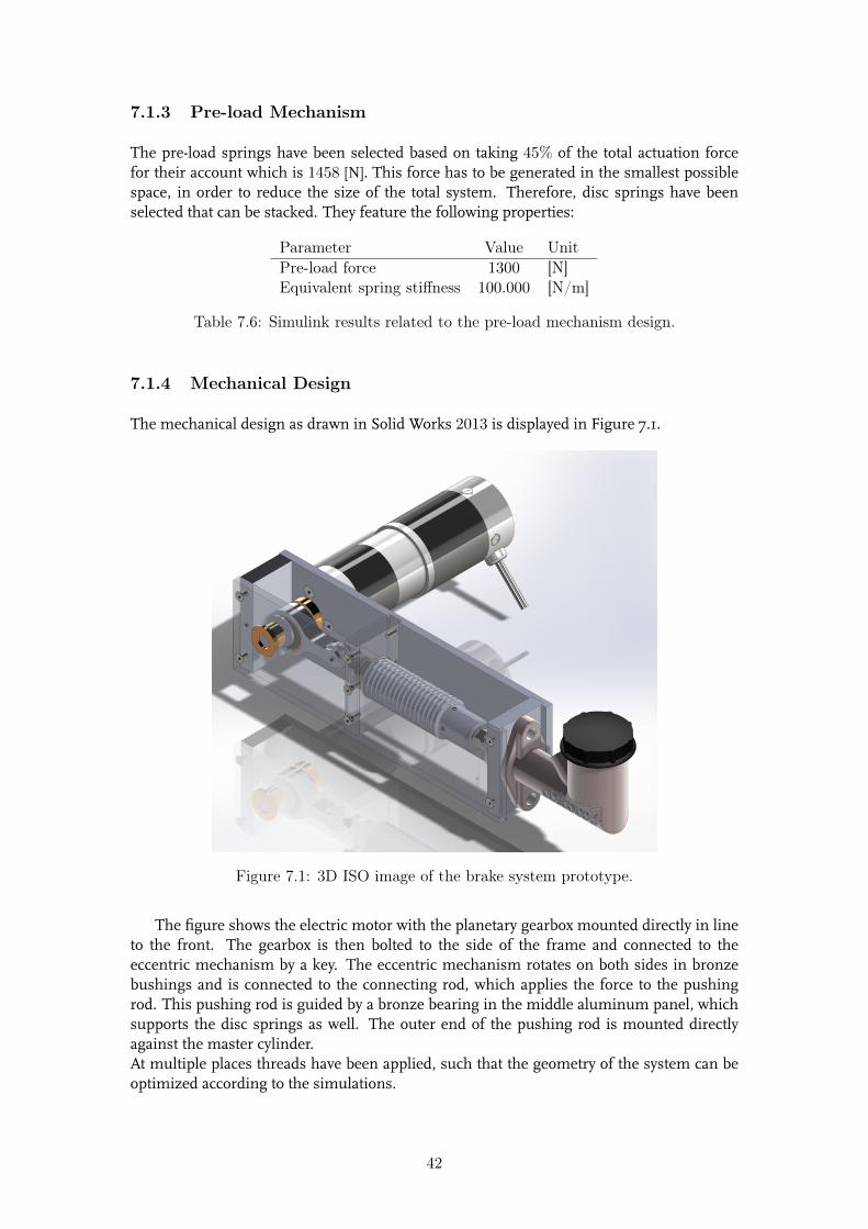
7.1.3 Pre-load Mechanism

The pre-load springs have been selected based on taking 45% of the total actuation forcefor their account which is 1458 [N]. This force has to be generated in the smallest possiblespace, in order to reduce the size of the total system. Therefore, disc springs have beenselected that can be stacked. They feature the following properties:

Parameter Value UnitPre-load force 1300 [N]Equivalent spring stiffness 100.000 [N/m]

Table 7.6: Simulink results related to the pre-load mechanism design.

7.1.4 Mechanical Design

The mechanical design as drawn in Solid Works 2013 is displayed in Figure 7.1.

Figure 7.1: 3D ISO image of the brake system prototype.

The figure shows the electric motor with the planetary gearbox mounted directly in lineto the front. The gearbox is then bolted to the side of the frame and connected to theeccentric mechanism by a key. The eccentric mechanism rotates on both sides in bronzebushings and is connected to the connecting rod, which applies the force to the pushingrod. This pushing rod is guided by a bronze bearing in the middle aluminum panel, whichsupports the disc springs as well. The outer end of the pushing rod is mounted directlyagainst the master cylinder.At multiple places threads have been applied, such that the geometry of the system can beoptimized according to the simulations.

42

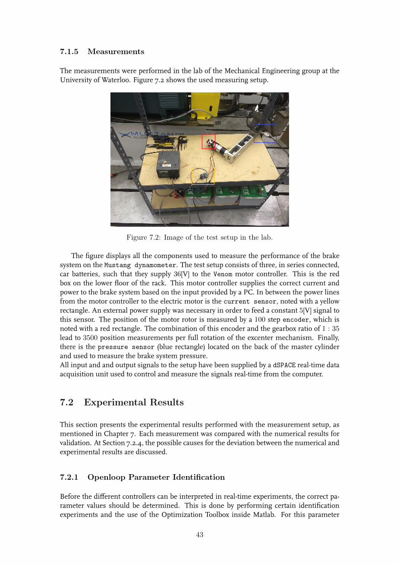
7.1.5 Measurements

The measurements were performed in the lab of the Mechanical Engineering group at theUniversity of Waterloo. Figure 7.2 shows the used measuring setup.

Figure 7.2: Image of the test setup in the lab.

The figure displays all the components used to measure the performance of the brakesystem on the Mustang dynamometer. The test setup consists of three, in series connected,car batteries, such that they supply 36[V] to the Venom motor controller. This is the redbox on the lower floor of the rack. This motor controller supplies the correct current andpower to the brake system based on the input provided by a PC. In between the power linesfrom the motor controller to the electric motor is the current sensor, noted with a yellowrectangle. An external power supply was necessary in order to feed a constant 5[V] signal tothis sensor. The position of the motor rotor is measured by a 100 step encoder, which isnoted with a red rectangle. The combination of this encoder and the gearbox ratio of 1 : 35lead to 3500 position measurements per full rotation of the excenter mechanism. Finally,there is the pressure sensor (blue rectangle) located on the back of the master cylinderand used to measure the brake system pressure.All input and and output signals to the setup have been supplied by a dSPACE real-time dataacquisition unit used to control and measure the signals real-time from the computer.

7.2 Experimental Results

This section presents the experimental results performed with the measurement setup, asmentioned in Chapter 7. Each measurement was compared with the numerical results forvalidation. At Section 7.2.4, the possible causes for the deviation between the numerical andexperimental results are discussed.

7.2.1 Openloop Parameter Identification

Before the different controllers can be interpreted in real-time experiments, the correct pa-rameter values should be determined. This is done by performing certain identificationexperiments and the use of the Optimization Toolbox inside Matlab. For this parameter

43

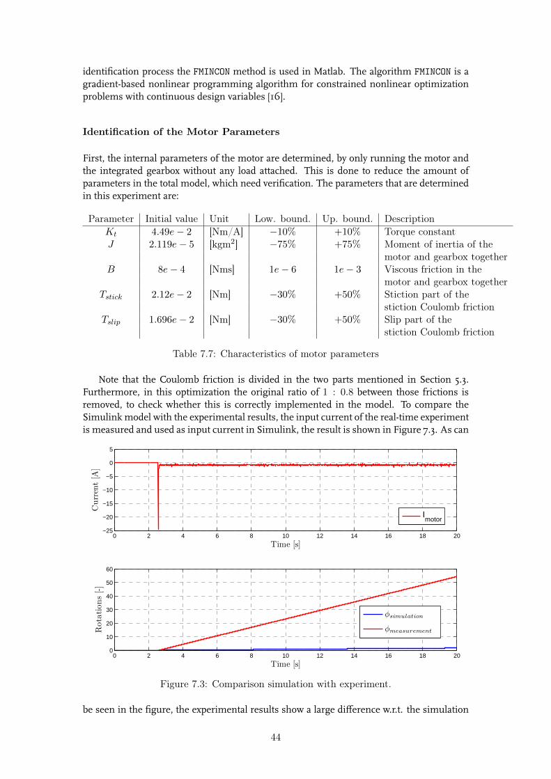
identification process the FMINCON method is used in Matlab. The algorithm FMINCON is agradient-based nonlinear programming algorithm for constrained nonlinear optimizationproblems with continuous design variables [16].

Identification of the Motor Parameters

First, the internal parameters of the motor are determined, by only running the motor andthe integrated gearbox without any load attached. This is done to reduce the amount ofparameters in the total model, which need verification. The parameters that are determinedin this experiment are:

Parameter Initial value Unit Low. bound. Up. bound. DescriptionKt 4.49e− 2 [Nm/A] −10% +10% Torque constantJ 2.119e− 5 [kgm2] −75% +75% Moment of inertia of the

motor and gearbox togetherB 8e− 4 [Nms] 1e− 6 1e− 3 Viscous friction in the

motor and gearbox togetherTstick 2.12e− 2 [Nm] −30% +50% Stiction part of the

stiction Coulomb frictionTslip 1.696e− 2 [Nm] −30% +50% Slip part of the

stiction Coulomb friction

Table 7.7: Characteristics of motor parameters

Note that the Coulomb friction is divided in the two parts mentioned in Section 5.3.Furthermore, in this optimization the original ratio of 1 : 0.8 between those frictions isremoved, to check whether this is correctly implemented in the model. To compare theSimulink model with the experimental results, the input current of the real-time experimentis measured and used as input current in Simulink, the result is shown in Figure 7.3. As can

0 2 4 6 8 10 12 14 16 18 20−25

−20

−15

−10

−5

0

5

Time [s]

Current[A

]

0 2 4 6 8 10 12 14 16 18 200

10

20

30

40

50

60

Time [s]

Rotations[-]

Imotor

φsimulation

φmeasurement

Figure 7.3: Comparison simulation with experiment.

be seen in the figure, the experimental results show a large difference w.r.t. the simulation

44

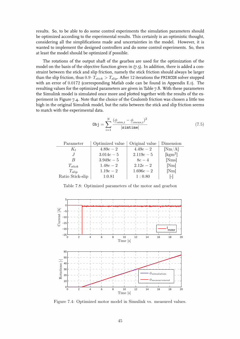
results. So, to be able to do some control experiments the simulation parameters shouldbe optimized according to the experimental results. This certainly is an optimistic thought,considering all the simplifications made and uncertainties in the model. However, it iswanted to implement the designed controllers and do some control experiments. So, thenat least the model should be optimized if possible.

The rotations of the output shaft of the gearbox are used for the optimization of themodel on the basis of the objective function given in (7.5). In addition, there is added a con-straint between the stick and slip friction, namely the stick friction should always be largerthan the slip friction, thus 0.9 ·Tstick > Tslip. After 12 iterations the FMINCON solver stoppedwith an error of 0.0172 (corresponding Matlab code can be found in Appendix E.1). Theresulting values for the optimized parameters are given in Table 7.8. With these parametersthe Simulink model is simulated once more and plotted together with the results of the ex-periment in Figure 7.4. Note that the choice of the Coulomb friction was chosen a little toohigh in the original Simulink model, but the ratio between the stick and slip friction seemsto match with the experimental data.

Obj =N∑i=1

(φsim,i

− φmeas,i

)2

|simtime|(7.5)

Parameter Optimized value Original value DimensionKt 4.89e− 2 4.49e− 2 [Nm/A]J 3.014e− 5 2.119e− 5 [kgm2]B 3.949e− 5 8e− 4 [Nms]

Tstick 1.48e− 2 2.12e− 2 [Nm]Tslip 1.19e− 2 1.696e− 2 [Nm]

Ratio Stick-slip 1:0.81 1 : 0.80 [-]

Table 7.8: Optimized parameters of the motor and gearbox

0 2 4 6 8 10 12 14 16 18 20−25

−20

−15

−10

−5

0

5

Time [s]

Current[A

]

Imotor

0 2 4 6 8 10 12 14 16 18 200

10

20

30

40

50

60

Time [s]

Rotations[-]

φsimulation

φmeasurement

Figure 7.4: Optimized motor model in Simulink vs. measured values.

45

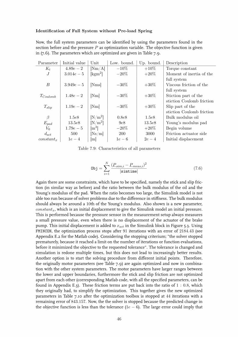
Identification of Full System without Pre-load Spring

Now, the full system parameters can be identified by using the parameters found in thesection before and the pressure P as optimization variable. The objective function is givenin (7.6). The parameters which are optimized are given in Table 7.9.

Parameter Initial value Unit Low. bound. Up. bound. DescriptionKt 4.89e− 2 [Nm/A] −10% +10% Torque constantJ 3.014e− 5 [kgm2] −20% +20% Moment of inertia of the

full systemB 3.949e− 5 [Nms] −30% +30% Viscous friction of the

full systemTCoulomb 1.48e− 2 [Nm] −30% +30% Stiction part of the

stiction Coulomb frictionTslip 1.19e− 2 [Nm] −30% +30% Slip part of the

stiction Coulomb frictionβ 1.5e8 [N/m2] 0.8e8 1.5e8 Bulk modulus oil

Epad 13.5e8 [N/m2] 9e8 13.5e8 Young’s modulus padV0 1.79e− 5 [m3] −20% +20% Begin volumedact 500 [Ns/m] 200 3000 Friction actuator side

constantx 1e− 4 [m] 1e− 6 2e− 4 Initial displacement

Table 7.9: Characteristics of all parameters

Obj =

N∑i=1

(P sim,i − Pmeas,i)2

|simtime|(7.6)

Again there are some constraints, which have to be specified, namely the stick and slip fric-tion (in similar way as before) and the ratio between the bulk modulus of the oil and theYoung’s modulus of the pad. When the ratio becomes too large, the Simulink model is notable too run because of solver problems due to the difference in stiffness. The bulk modulusshould always be around a 10th of the Young’s modulus. Also shown is a new parameter,constantx, which is an initial displacement to give the Simulink model an initial pressure.This is performed because the pressure sensor in the measurement setup always measuresa small pressure value, even when there is no displacement of the actuator of the brakepump. This initial displacement is added to xact in the Simulink block in Figure 5.3. UsingFMINCON, the optimization process stops after 91 iterations with an error of 2184.43 (seeAppendix E.2 for the Matlab code). Considering the stopping criterium; "the solver stoppedprematurely, because it reached a limit on the number of iterations or function evaluations,before it minimized the objective to the requested tolerance". The tolerance is changed andsimulation is redone multiple times, but this does not lead to increasingly better results.Another option is to start the solving procedure from different initial points. Therefore,the originally motor parameters (see Table 7.9) are again optimized and now in combina-tion with the other system parameters. The motor parameters have larger ranges betweenthe lower and upper boundaries, furthermore the stick and slip friction are not optimizedapart from each other (corresponding Matlab code, with all the specified parameters, can befound in Appendix E.3). These friction terms are put back into the ratio of 1 : 0.8, whichthey originally had, to simplify the optimization. This together gives the new optimizedparameters in Table 7.10 after the optimization toolbox is stopped at 44 iterations with aremaining error of 843.157. Now, the the solver is stopped because the predicted change inthe objective function is less than the tolerance (1e − 6). The large error could imply that

46

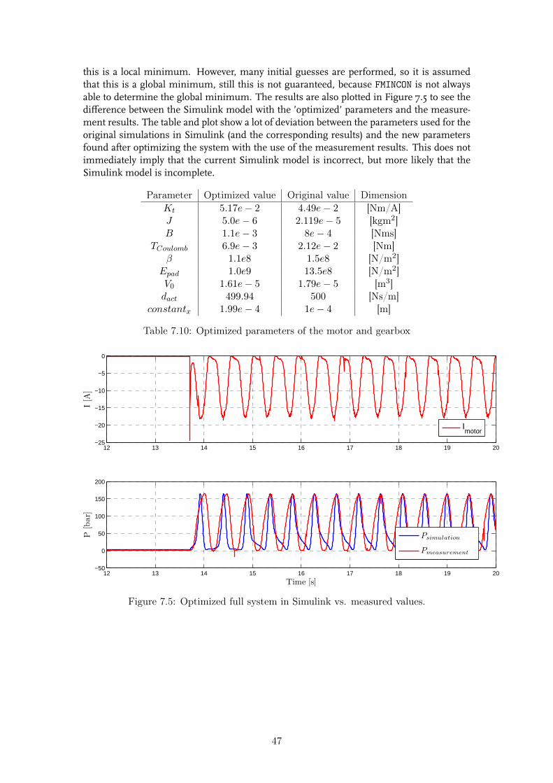
this is a local minimum. However, many initial guesses are performed, so it is assumedthat this is a global minimum, still this is not guaranteed, because FMINCON is not alwaysable to determine the global minimum. The results are also plotted in Figure 7.5 to see thedifference between the Simulink model with the ’optimized’ parameters and the measure-ment results. The table and plot show a lot of deviation between the parameters used for theoriginal simulations in Simulink (and the corresponding results) and the new parametersfound after optimizing the system with the use of the measurement results. This does notimmediately imply that the current Simulink model is incorrect, but more likely that theSimulink model is incomplete.

Parameter Optimized value Original value DimensionKt 5.17e− 2 4.49e− 2 [Nm/A]J 5.0e− 6 2.119e− 5 [kgm2]B 1.1e− 3 8e− 4 [Nms]

TCoulomb 6.9e− 3 2.12e− 2 [Nm]β 1.1e8 1.5e8 [N/m2]

Epad 1.0e9 13.5e8 [N/m2]V0 1.61e− 5 1.79e− 5 [m3]dact 499.94 500 [Ns/m]

constantx 1.99e− 4 1e− 4 [m]

Table 7.10: Optimized parameters of the motor and gearbox

12 13 14 15 16 17 18 19 20−25

−20

−15

−10

−5

0

I[A

]

Imotor

12 13 14 15 16 17 18 19 20−50

0

50

100

150

200

Time [s]

P[bar]

Psimulation

Pmeasurement

Figure 7.5: Optimized full system in Simulink vs. measured values.

47

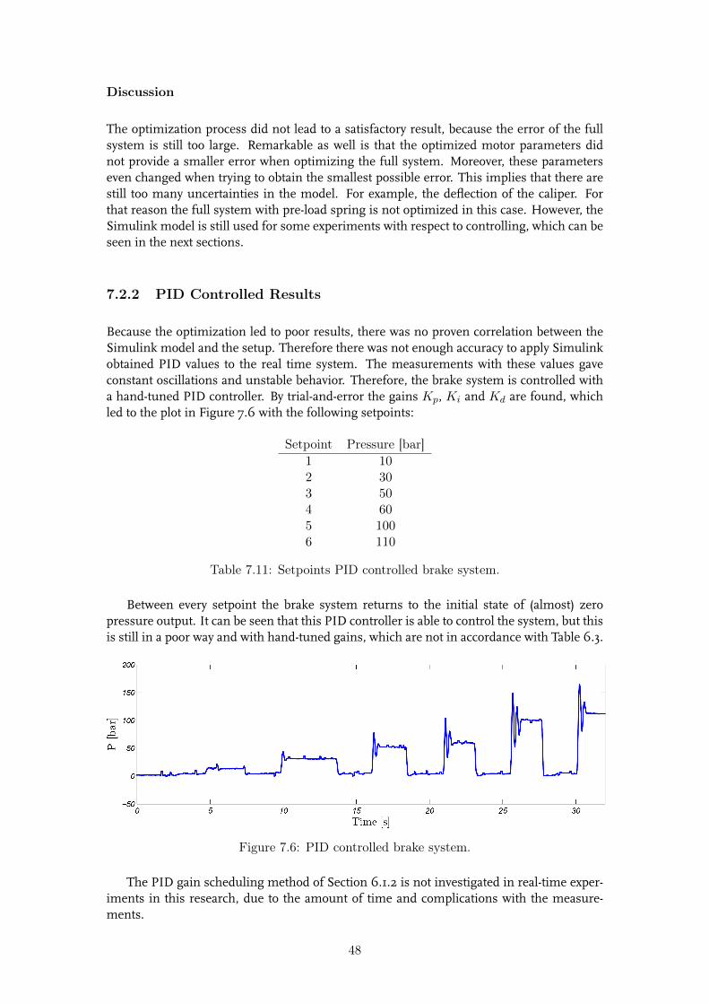
Discussion

The optimization process did not lead to a satisfactory result, because the error of the fullsystem is still too large. Remarkable as well is that the optimized motor parameters didnot provide a smaller error when optimizing the full system. Moreover, these parameterseven changed when trying to obtain the smallest possible error. This implies that there arestill too many uncertainties in the model. For example, the deflection of the caliper. Forthat reason the full system with pre-load spring is not optimized in this case. However, theSimulink model is still used for some experiments with respect to controlling, which can beseen in the next sections.

7.2.2 PID Controlled Results

Because the optimization led to poor results, there was no proven correlation between theSimulink model and the setup. Therefore there was not enough accuracy to apply Simulinkobtained PID values to the real time system. The measurements with these values gaveconstant oscillations and unstable behavior. Therefore, the brake system is controlled witha hand-tuned PID controller. By trial-and-error the gains Kp, Ki and Kd are found, whichled to the plot in Figure 7.6 with the following setpoints:

Setpoint Pressure [bar]1 102 303 504 605 1006 110

Table 7.11: Setpoints PID controlled brake system.

Between every setpoint the brake system returns to the initial state of (almost) zeropressure output. It can be seen that this PID controller is able to control the system, but thisis still in a poor way and with hand-tuned gains, which are not in accordance with Table 6.3.

Figure 7.6: PID controlled brake system.

The PID gain scheduling method of Section 6.1.2 is not investigated in real-time exper-iments in this research, due to the amount of time and complications with the measure-ments.

48

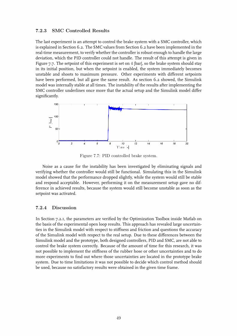
7.2.3 SMC Controlled Results

The last experiment is an attempt to control the brake system with a SMC controller, whichis explained in Section 6.2. The SMC values from Section 6.2 have been implemented in thereal-time measurement, to verify whether the controller is robust enough to handle the largedeviation, which the PID controller could not handle. The result of this attempt is given inFigure 7.7. The setpoint of this experiment is set on 4 [bar], so the brake system should stayin its initial position, but when the setpoint is enabled, the system immediately becomesunstable and shoots to maximum pressure. Other experiments with different setpointshave been performed, but all gave the same result. As section 6.2 showed, the Simulinkmodel was internally stable at all times. The instability of the results after implementing theSMC controller underlines once more that the actual setup and the Simulink model differsignificantly.

Figure 7.7: PID controlled brake system.

Noise as a cause for the instability has been investigated by eliminating signals andverifying whether the controller would still be functional. Simulating this in the Simulinkmodel showed that the performance dropped slightly, while the system would still be stableand respond acceptable. However, performing it on the measurement setup gave no dif-ference in achieved results, because the system would still become unstable as soon as thesetpoint was activated.

7.2.4 Discussion

In Section 7.2.1, the parameters are verified by the Optimization Toolbox inside Matlab onthe basis of the experimental open loop results. This approach has revealed large uncertain-ties in the Simulink model with respect to stiffness and friction and questions the accuracyof the Simulink model with respect to the real setup. Due to these differences between theSimulink model and the prototype, both designed controllers, PID and SMC, are not able tocontrol the brake system correctly. Because of the amount of time for this research, it wasnot possible to implement the stiffness of the rubber hose or other uncertainties and to domore experiments to find out where those uncertainties are located in the prototype brakesystem. Due to time limitations it was not possible to decide which control method shouldbe used, because no satisfactory results were obtained in the given time frame.

49

50

Chapter 8

Conclusion and Recommendations

In this chapter we present the conclusion of this research, recommendations and areas offuture research.

8.1 Conclusion

Conclusions based on the (control) simulations and the experimental results are discussedin this section. The goal of this project to build a small electric brake system capable ofachieving 120 [bar] brake pressure in 50 [ms] has not been achieved. The simulationsshowed promising results, because they met the requirements, still reasonable because ofcertain simplifications. Furthermore, the experimental results were not in accordance withthese simulation results. The identified causes contributing to this deviation are discussedin the following section.

8.2 Recommendations

The following recommendations are proposed to improve the experimental method:

• The friction in the system is currently modeled as a combination of stick-slip and vis-cous friction. The total friction model should include Stribeck friction as well. Exper-iments need to be executed to determine this type of friction and get a more accuratefriction model.

• The stiffness of the brake caliper should be incorporated in the Simulink model. Thedeflection of the caliper under 120 [bar] pressure showed to be quite substantial in therange of tenth’s of millimeters. This was observed during the experimental measure-ments.

• The expansion of the brake hose under fluid pressure should be incorporated in theSimulink model. It was observed during experimental measurements that under in-creasing pressure the brake hose moves around slightly due to internal elongations.

• Reflecting the already mentioned recommendations; perform a total model identifi-cation to determine an accurate Simulink model, which is consistent with the realsetup.

• Perform a proper and more extensive parameter optimization, since the optimizationin this research was not competent and complete enough to get satisfying results.

51

• The current prototype used to validate the proposed system has focussed too much ona minimal size and therefore some unforseen bending and movement of componentsoccurred during operation. An improved prototype should be designed such that theseundesired effects do not occur during operation and a proper proof of concept couldbe performed.

52

Bibliography

[1] T. Gilles. Automotive Chassis: Brakes, Suspension, and Steering. Thomson Delmar Learn-ing, Clifton Park, United States, 2005.

[2] S.B. Choi and D. Milot. An anti-lock brake system with continuous wheel slip control,April 18 2012. EP Patent 1,603,781.

[3] Robert Bosch GmbH. BOSCH Automotive Handbook. Bosch Handbooks. Wiley, 2004.

[4] U. Stoll. Sensotronic brake control (sbc) - the electro-hydraulic brake from mercedes-benz. VDI Berichte, 1789:675–685, 2003.

[5] J. Sakamoto A. Otomo" "M. Soga, M. Shimada. Development of vehicle dynamicsmanagement system for hybrid vehicles: Ecb system for improved environmental andvehicle dynamic performance. JSAE Review, 23(4):459–464, 2002.

[6] T. Tamasho, M. Kubota, and M. Tsukamoto. Electromechanical brake system, June 42002. US Patent 6,397,981.

[7] J. van der Walt" "S. Saric, A. Bab-Hadiashar. Estimating clamp force for brake-by-wiresystems: Thermal considerations. Mechatronics, 19(6):886 – 895, 2009.

[8] Laaleh Durali. A new individual wheel actuated braking system to improve reliabilityand vehicle stability. University of Waterloo, PhD proposal, 1(1):1–60, 2013.

[9] J. Sarangapani. Neural Network Control of Nonlinear Discrete-Time Systems. Automationand Control Engineering. Taylor & Francis, 2006.

[10] Ivan Virgala and Mlcria Kenderovlc, Peter Frankovsky. Friction effect analysis of a dcmotor. American Journal of Mechanical Engineering, 1(1):1–5, 2013.

[11] The Mathworks Inc. Rotational friction, year = 2014, url =http://nl.mathworks.com/help/physmod/simscape/ref/rotationalfriction.html.

[12] S. Skogestad. Probably the best simple pid tuning rules in the world. Journal of ProcessControl, 1(1):1–27, 2001.

[13] W.K. Ho, O.P. Gan, E.B. Tay, and E.L. Ang. Performance and gain and phase marginsof well-known pid tuning formulas. Control Systems Technology, IEEE Transactions on,4(4):473–477, Jul 1996.

[14] Sigurd Skogestad. Probably the best simple pid tuning rules in the world. In AIChEAnnual Meeting, Reno, Nevada, 2001.

[15] KM Arun Prasad, Bindu M Krishna, and Usha Nair. Modified chattering free slid-ing mode control of dc motor. International Journal of Modern Engineering Research(IJMER), 3, May-Jun 2013.

[16] P.Y. Papalambros and D.J. Wilde. Principles of Optimal Design: Modeling and Computa-tion, volume 1, 2nd edition. Cambridge University Press, 2000.

53

54

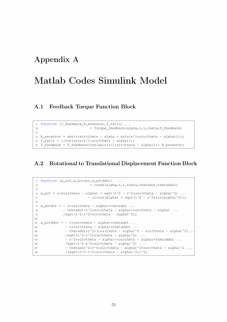
Appendix A

Matlab Codes Simulink Model

A.1 Feedback Torque Function Block

1 function [T_feedback,R_excenter,f_ratio] ...2 = Torque_feedback(alpha,r,l,theta,F_feedback)3

4 R_excenter = abs(r*sin(theta - alpha + asin(r/l*sin(theta - alpha))));5 f_ratio = 1/cos(asin(r/l*sin(theta - alpha)));6 T_feedback = F_feedback/cos(asin(r/l*sin(theta - alpha)))* R_excenter;

A.2 Rotational to Translational Displacement Function Block

1 function [x_act,x_actdot,x_actddot] ...2 = crank(alpha,r,l,theta,thetadot,thetaddot)3

4 x_act = r*cos(theta - alpha) + sqrt(l^2 - r^2*sin(theta - alpha)^2) ...5 - (r*cos(alpha) + sqrt(l^2 - r^2*sin(alpha)^2));6

7 x_actdot = - r*sin(theta - alpha)*thetadot ...8 - thetadot*r^2*sin(theta - alpha)*cos(theta - alpha) ...9 /sqrt(l^2-r^2*sin(theta - alpha)^2);

10

11 x_actddot = - r*cos(theta - alpha)*thetadot ...12 - r*sin(theta - alpha)*thetaddot ...13 - thetadot*r^2*(cos(theta - alpha)^2 - sin(theta - alpha)^2)...14 /sqrt(l^2-r^2*sin(theta - alpha)^2) ...15 - r^2*sin(theta - alpha)*cos(theta - alpha)*thetaddot ...16 /sqrt(l^2-r^2*sin(theta - alpha)^2) ...17 - thetadot^2*r^4*sin(theta - alpha)^2*cos(theta - alpha)^2 ...18 /(sqrt(l^2-r^2*sin(theta - alpha)^2))^3;

55

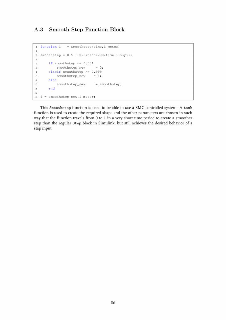
A.3 Smooth Step Function Block

1 function i = Smoothstep(time,i_motor)2

3 smoothstep = 0.5 + 0.5*tanh(200*time-1.5*pi);4

5 if smoothstep <= 0.0016 smoothstep_new = 0;7 elseif smoothstep >= 0.9998 smoothstep_new = 1;9 else

10 smoothstep_new = smoothstep;11 end12

13 i = smoothstep_new*i_motor;

This Smoothstep function is used to be able to use a SMC controlled system. A tanhfunction is used to create the required shape and the other parameters are chosen in suchway that the function travels from 0 to 1 in a very short time period to create a smootherstep than the regular Step block in Simulink, but still achieves the desired behavior of astep input.

56

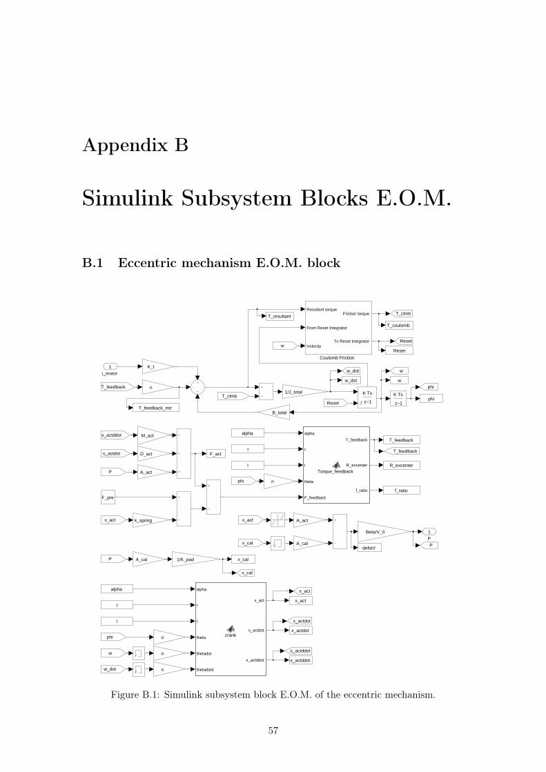
Appendix B

Simulink Subsystem Blocks E.O.M.

B.1 Eccentric mechanism E.O.M. block

P1

w_dot w

deltaV

x_actddot

x_cal

phi

T_feedback

x_actdot

Reset

T_resultant

T_coulomb

f_ratio

R_excenter

x_act

F_act

T_feedback_mtr

alpha

r

l

theta

F_feedback

T_feedback

R_excenter

f_ratio

Torque_feedback

alpha

r

l

theta

thetadot

thetaddot

x_act

x_actdot

x_actddot

crank

x_actddot

T_feedback

phi

ww_dot

P

x_act

x_cal

Reset

T_clmb

x_actdot

A_act

n

n

A_cal

n

n

1/K_pad

A_act

n

M_act

D_act

B_total

1/J_total

K_t

Beta/V_0

A_cal

k_spring

x_actdot

phi

P

x_act

T_feedback

P

x_act

x_cal

Reset

T_clmb

x_actddot

w

w

w_dot

phi

K Ts

z−1

K Ts

z−1

Coulomb Friction

Resultant torque

From Reset Integrator

Velocity

Friction torque

To Reset Integrator

r

alpha

l

r

alpha

l

F_pre

i_motor1

Figure B.1: Simulink subsystem block E.O.M. of the eccentric mechanism.

57

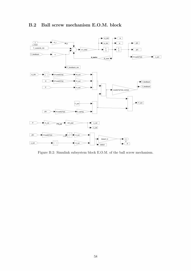
B.2 Ball screw mechanism E.O.M. block

P1

w_dot w

deltaV

x_cal

phi

T_feedback

x_act

F_act

T_feedback_mtr

1s

1s

T_feedback

phi

ww_dot

P

x_cal

A_act

A_cal

n

1/K_pad

n*Lead/(2*pi)

n*Lead/(2*pi)

n*Lead/(2*pi)

n*Lead/(2*pi)

A_act

Lead/(2*pi*eta_screw)

M_act

D_act

n*Lead/(2*pi)

B_total

1/J_total

K_t

Beta/V_0

A_cal

k_spring

w

phi

P

phi

T_feedback

P

x_cal

w_dot

T_coulomb_mtr

F_pre

i_motor

1i*K_ti*K_t

x_act

P*A_calP*A_cal

B_total*wB_total*w

Figure B.2: Simulink subsystem block E.O.M. of the ball screw mechanism.

58

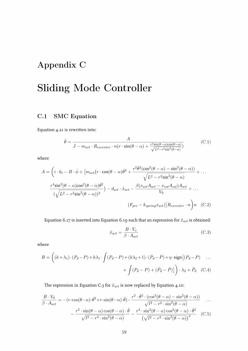
Appendix C

Sliding Mode Controller

C.1 SMC Equation

Equation 4.21 is rewritten into:

θ =A

J −mact ·Rexcenter · n(r · sin(θ − α) + r2sin(θ−α)cos(θ−α)√L2−r2sin2(θ−α)

)(C.1)

where

A =

(i · kt −B · φ+

[mact

(r · cos(θ − α)θ2 + r2θ2(cos2(θ − α)− sin2(θ − α))√

L2 − r2sin2(θ − α)+ . . .

r4sin2(θ − α)cos2(θ − α)θ2

(√L2 − r2sin2(θ − α))3

)− dact · xact −

β(xactAact − xcalAcal)AactV0

+ . . .

(Fpre − kspringxact)]Rexcenter · n

)n (C.2)

Equation 6.17 is inserted into Equation 6.19 such that an expression for xact is obtained:

xact =B · Voβ ·Aact

(C.3)

where

B =

((k+λ1) ·(Pd−P )+kλ1 ·

∫(Pd−P )+(kλ2+1) ·(Pd− P )+η ·sign

[(Pd−P ) . . .

+

∫(Pd − P ) + (Pd − P )

])· λ2 + Pd (C.4)

The expression in Equation C.3 for xact is now replaced by Equation 4.10:

B · V0β ·Aact

= −(r·cos(θ−α)·θ2+r·sin(θ−α)·θ)− r2 · θ2 · (cos2(θ − α)− sin2(θ − α))√

l2 − r2 · sin2(θ − α). . .

− r2 · sin(θ − α) cos(θ − α) · θ√l2 − r2 · sin2(θ − α)

− r4 · sin2(θ − α) cos2(θ − α) · θ2(√l2 − r2 · sin2(θ − α)

)3 (C.5)

59

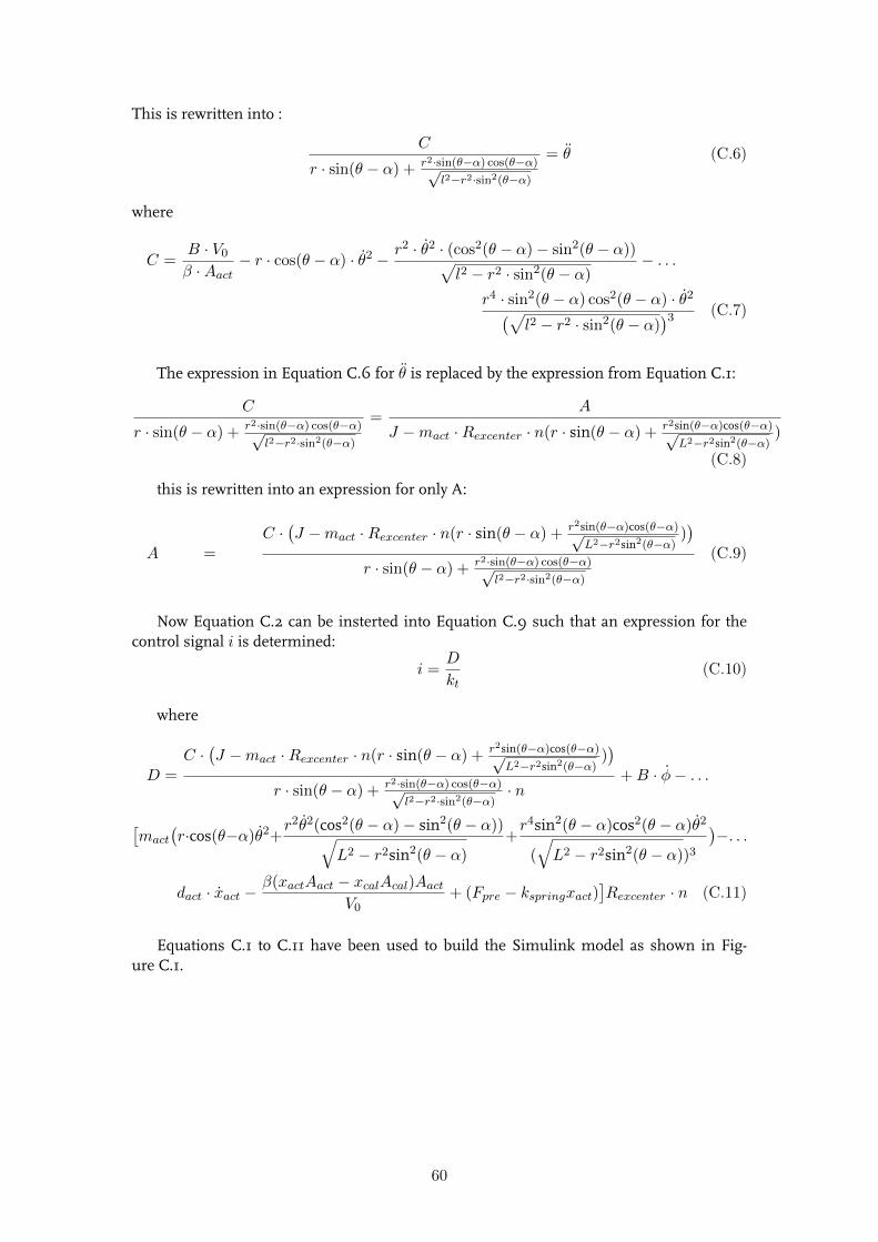
This is rewritten into :

C

r · sin(θ − α) + r2·sin(θ−α) cos(θ−α)√l2−r2·sin2(θ−α)

= θ (C.6)

where

C =B · V0β ·Aact

− r · cos(θ − α) · θ2 − r2 · θ2 · (cos2(θ − α)− sin2(θ − α))√l2 − r2 · sin2(θ − α)

− . . .

r4 · sin2(θ − α) cos2(θ − α) · θ2(√l2 − r2 · sin2(θ − α)

)3 (C.7)

The expression in Equation C.6 for θ is replaced by the expression from Equation C.1:

C

r · sin(θ − α) + r2·sin(θ−α) cos(θ−α)√l2−r2·sin2(θ−α)

=A

J −mact ·Rexcenter · n(r · sin(θ − α) + r2sin(θ−α)cos(θ−α)√L2−r2sin2(θ−α)

)

(C.8)

this is rewritten into an expression for only A:

A =C ·(J −mact ·Rexcenter · n(r · sin(θ − α) + r2sin(θ−α)cos(θ−α)√

L2−r2sin2(θ−α)))

r · sin(θ − α) + r2·sin(θ−α) cos(θ−α)√l2−r2·sin2(θ−α)

(C.9)

Now Equation C.2 can be insterted into Equation C.9 such that an expression for thecontrol signal i is determined:

i =D

kt(C.10)

where

D =C ·(J −mact ·Rexcenter · n(r · sin(θ − α) + r2sin(θ−α)cos(θ−α)√

L2−r2sin2(θ−α)))

r · sin(θ − α) + r2·sin(θ−α) cos(θ−α)√l2−r2·sin2(θ−α)

· n+B · φ− . . .

[mact

(r·cos(θ−α)θ2+r

2θ2(cos2(θ − α)− sin2(θ − α))√L2 − r2sin2(θ − α)

+r4sin2(θ − α)cos2(θ − α)θ2

(√L2 − r2sin2(θ − α))3

)−. . .

dact · xact −β(xactAact − xcalAcal)Aact

V0+ (Fpre − kspringxact)

]Rexcenter · n (C.11)

Equations C.1 to C.11 have been used to build the Simulink model as shown in Fig-ure C.1.

60

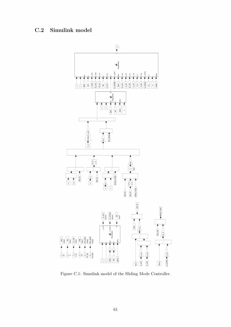
C.2 Simulink model

i1

Sig

n

r l phi

w J_to

tal

B_t

otal

m_a

ct

R d_ac

t

B x_ac

tdot

Bet

a

x_ac

t

A_a

ct

x_ca

l

A_c

al

V_0

F_p

re

k_sp

ring

K_t

n alph

a

iP

aram

eter

s

A r l phi

w alph

a

n

B

Par

amet

ers

r l phi

w alph

a

x_ac

t

x_ac

tdot R

Par

amet

ers

Got

o9[phi

]

Got

o8

[Pd_

ddot

]

Got

o7[R]

Got

o6

[Pd_

dot]

Got

o4[Pd]

Got

o2

[x_c

al]

Got

o13

[x_a

ct]

[Pdd

ot_P

dot]

Got

o11

[x_a

ctdo

t]

[Pd_

P]

Got

o1[w]

A_a

ct

Eta

1/L2

L2

L1

n n

1/V

_0

1/V

_0

1/(B

eta*

A_a

ct)

A_c

al

A_a

ct

[Pd_

ddot

]

[Pdd

ot_P

dot]

[phi

]

[w]

[phi

]

[x_c

al]

[x_a

ct]

[Pd_

P]

[Pdd

ot_P

dot]

[Pd_

P]

[Pd_

P]

[R]

[x_a

ctdo

t]

[x_c

al]

[x_a

ct]

[w]

[phi

]

[w]

[x_a

ctdo

t]

[Pd_

dot]

[Pd_

P]

[Pd]

K T

s

z−1

K T

s

z−1

r

1Kl

K

Bet

a

L1

alph

a

n

n

alph

a

K_t

k_sp

ring

F_p

re

V_0

A_c

al

A_a

ct

K

V_0

Bet

a

d_ac

t

M_a

ct

lr

alph

a

B_t

otal

J_to

tal

l

r

Bet

a

Pd_

ddot

6

Pd_

dot

5Pd4

x_ca

l3w2ph

i

1

Figure C.1: Simulink model of the Sliding Mode Controller.

61

62

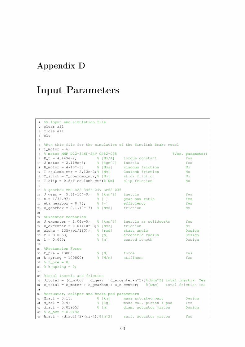
Appendix D

Input Parameters

1 %% Input and simulation file2 clear all3 close all4 clc5

6 %Run this file for the simulation of the Simulink Brake model7 i_motor = 6;8 % motor MMP D22-346F-24V GP52-035 %Ver. parameter:9 K_t = 4.449e-2; % [Nm/A] torque constant Yes

10 J_motor = 2.119e-5; % [kgm^2] inertia Yes11 B_motor = 4*10^-3; % [Nms] viscous friction No12 T_coulomb_mtr = 2.12e-2;% [Nm] Coulomb friction No13 T_stick = T_coulomb_mtr;% [Nm] stick friction No14 T_slip = 0.8*T_coulomb_mtr;%[Nm] slip friction No15

16 % gearbox MMP D22-346F-24V GP52-03517 J_gear = 5.31*10^-9; % [kgm^2] inertia Yes18 n = 1/34.97; % [-] gear box ratio Yes19 eta_gearbox = 0.75; % [-] efficiency Yes20 B_gearbox = 0.1*10^-3; % [Nms] friction No21

22 %Excenter mechanism23 J_excenter = 1.04e-5; % [kgm^2] inertia as solidworks Yes24 B_excenter = 0.01*10^-3;% [Nms] friction No25 alpha = 135*(pi/180); % [rad] start angle Design26 r = 0.0053; % [m] eccentric radius Design27 l = 0.045; % [m] conrod length Design28

29 %Pretension Force30 F_pre = 1300; % [N] force Yes31 k_spring = 100000; % [N/m] stiffness Yes32 % F_pre = 0;33 % k_spring = 0;34

35 %Total inertia and friction36 J_total = (J_motor + J_gear + J_excenter*n^2);%[kgm^2] total inertia Yes37 B_total = B_motor + B_gearbox + B_excenter; %[Nms] total friction Yes38

39 %Actuator, caliper and brake pad parameters40 M_act = 0.15; % [kg] mass actuated part Design41 M_cal = 0.9; % [kg] mass cal. piston + pad Yes42 d_act = 0.01905; % [m] diam. actuator piston Design43 % d_act = 0.014244 A_act = (d_act)^2*(pi/4);%[m^2] surf. actuator piston Yes

63

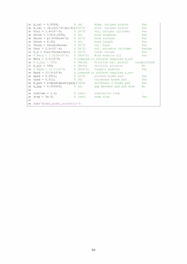
45 d_cal = 0.0599; % [m] diam. caliper piston Yes46 A_cal = (d_cal)^2*(pi/4);%[m^2] surf. caliper piston Yes47 Vcal = 1.4*10^-5; % [m^3] vol. caliper cylinder Yes48 Dhose = 1/8*0.0254; % [m] hose diameter Yes49 Ahose = pi/4*Dhose^2; % [m^2] hose surface Yes50 Lhose = 0.25; % [m] hose length Yes51 Vhose = Lhose*Ahose; % [m^3] vol. hose Yes52 Vact = 2.0*10^-6; % [m^3] vol. actuator cylinder Design53 V_0 = Vcal+Vhose+Vact; % [m^3] total volume Yes54 % Beta = 1.5234*10^9; % [N/m^2] Bulk modulus oil Yes55 Beta = 1.5*10^8; % Lowered to achieve required x_act56 % D_cal = 500; % [Ns/m] friction cal. piston (simplified)57 D_act = 500; % [Ns/m] friction actuator No58 % Epad = 13.5*10^9; % [N/m^2] Young's modulus Yes59 Epad = 13.5*10^8; % Lowered to achieve required x_act60 Apad = 0.0011; % [m^2] surface brake pad Yes61 tpad = 0.011; % [m] thickness brake pad Yes62 K_pad = 2*Epad*Apad/tpad;%[N/m] stiffness 2 brake pad Yes63 x_gap = 0.000005; % [m] gap between pad and disk No64

65 simtime = 1.5; % [sec] simulation time -66 step = 5e-3; % [sec] step size Yes67

68 sim('Brake_model_eccentric')

64

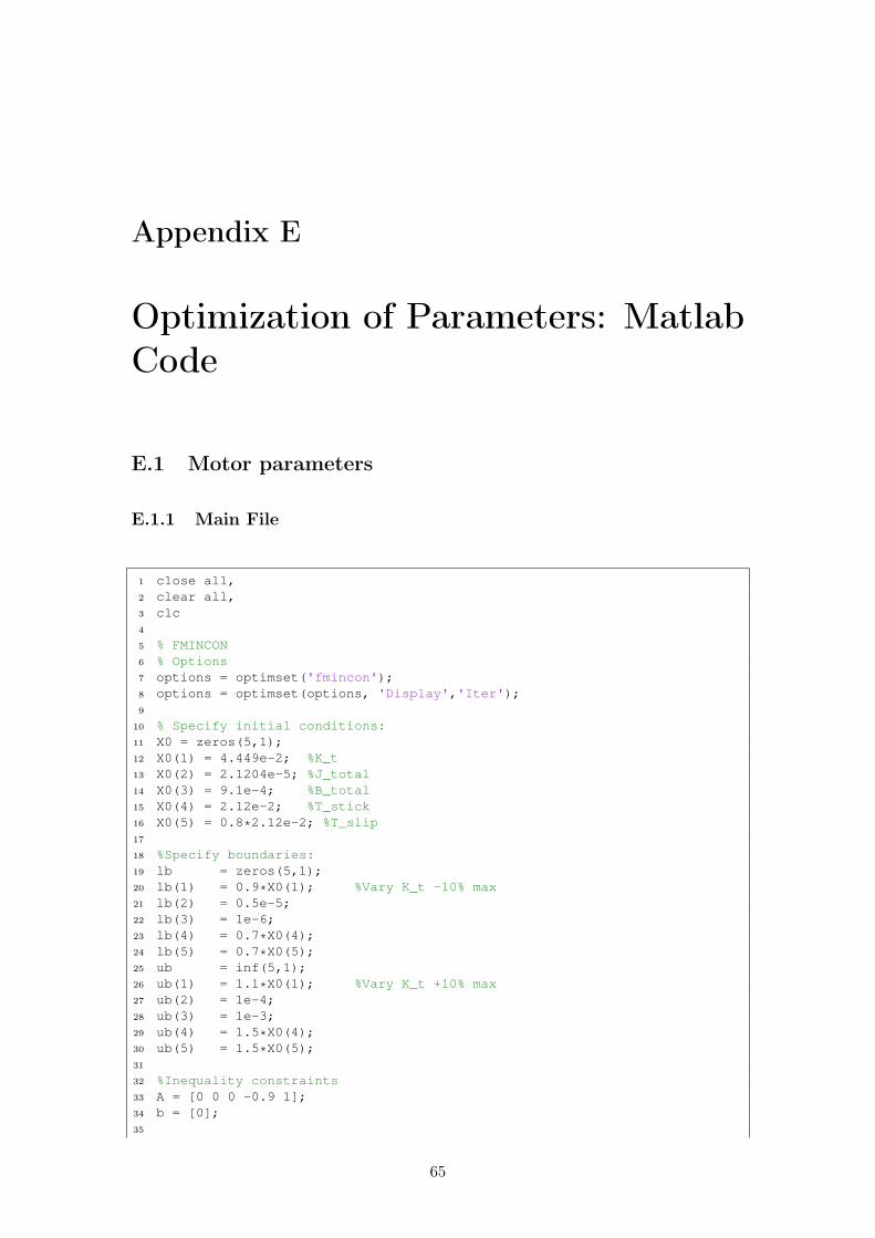
Appendix E

Optimization of Parameters: MatlabCode

E.1 Motor parameters

E.1.1 Main File

1 close all,2 clear all,3 clc4

5 % FMINCON6 % Options7 options = optimset('fmincon');8 options = optimset(options, 'Display','Iter');9

10 % Specify initial conditions:11 X0 = zeros(5,1);12 X0(1) = 4.449e-2; %K_t13 X0(2) = 2.1204e-5; %J_total14 X0(3) = 9.1e-4; %B_total15 X0(4) = 2.12e-2; %T_stick16 X0(5) = 0.8*2.12e-2; %T_slip17

18 %Specify boundaries:19 lb = zeros(5,1);20 lb(1) = 0.9*X0(1); %Vary K_t -10% max21 lb(2) = 0.5e-5;22 lb(3) = 1e-6;23 lb(4) = 0.7*X0(4);24 lb(5) = 0.7*X0(5);25 ub = inf(5,1);26 ub(1) = 1.1*X0(1); %Vary K_t +10% max27 ub(2) = 1e-4;28 ub(3) = 1e-3;29 ub(4) = 1.5*X0(4);30 ub(5) = 1.5*X0(5);31

32 %Inequality constraints33 A = [0 0 0 -0.9 1];34 b = [0];35

65

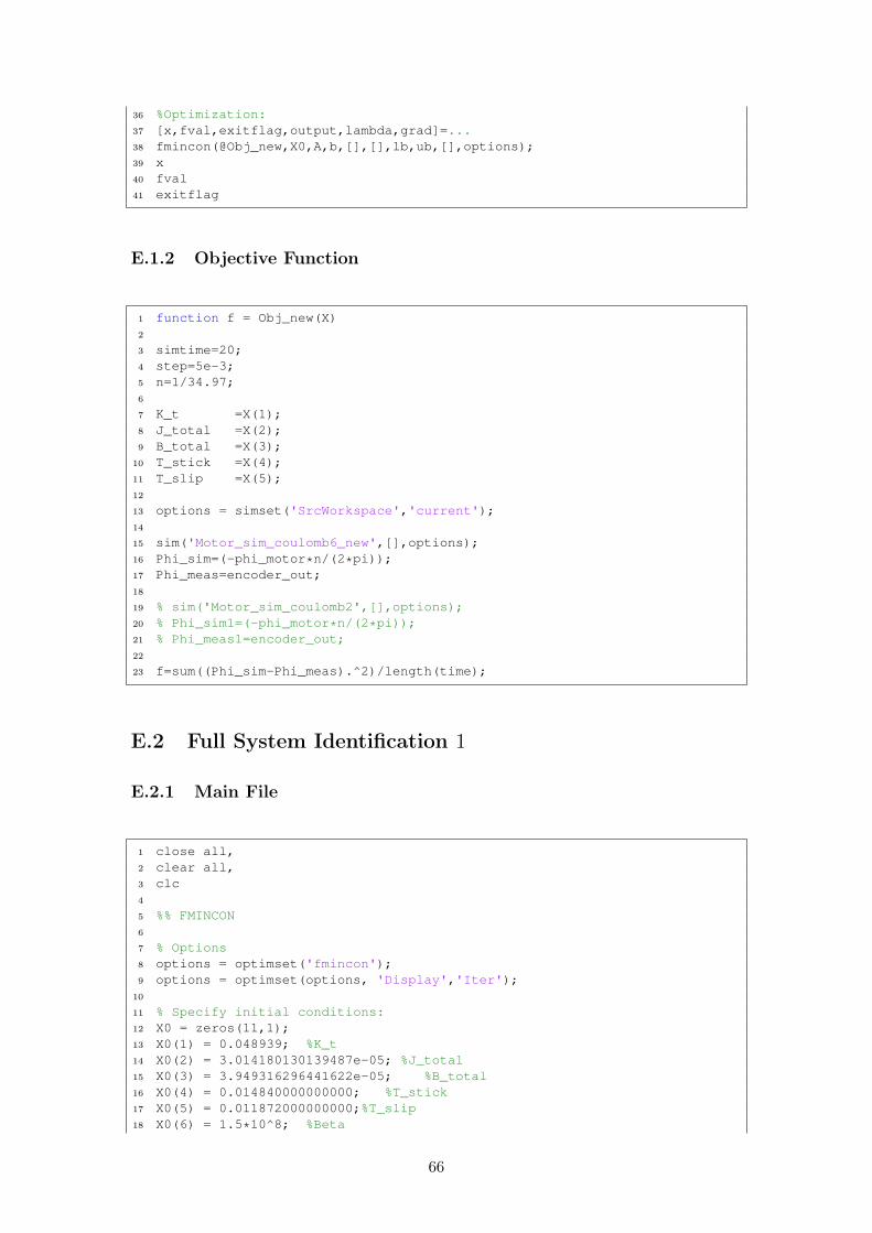
36 %Optimization:37 [x,fval,exitflag,output,lambda,grad]=...38 fmincon(@Obj_new,X0,A,b,[],[],lb,ub,[],options);39 x40 fval41 exitflag

E.1.2 Objective Function

1 function f = Obj_new(X)2

3 simtime=20;4 step=5e-3;5 n=1/34.97;6

7 K_t =X(1);8 J_total =X(2);9 B_total =X(3);

10 T_stick =X(4);11 T_slip =X(5);12

13 options = simset('SrcWorkspace','current');14

15 sim('Motor_sim_coulomb6_new',[],options);16 Phi_sim=(-phi_motor*n/(2*pi));17 Phi_meas=encoder_out;18

19 % sim('Motor_sim_coulomb2',[],options);20 % Phi_sim1=(-phi_motor*n/(2*pi));21 % Phi_meas1=encoder_out;22

23 f=sum((Phi_sim-Phi_meas).^2)/length(time);

E.2 Full System Identification 1

E.2.1 Main File

1 close all,2 clear all,3 clc4

5 %% FMINCON6

7 % Options8 options = optimset('fmincon');9 options = optimset(options, 'Display','Iter');

10

11 % Specify initial conditions:12 X0 = zeros(11,1);13 X0(1) = 0.048939; %K_t14 X0(2) = 3.014180130139487e-05; %J_total15 X0(3) = 3.949316296441622e-05; %B_total16 X0(4) = 0.014840000000000; %T_stick17 X0(5) = 0.011872000000000;%T_slip18 X0(6) = 1.5*10^8; %Beta

66

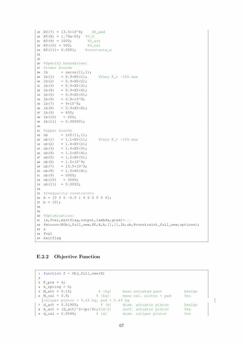
19 X0(7) = 13.5*10^8; %K_pad20 X0(8) = 1.79e-05; %V_021 X0(9) = 1000; %D_act22 X0(10) = 500; %D_cal23 X0(11)= 0.0001; %constante_x24

25

26 %Specify boundaries:27 %lower bounds28 lb = zeros(11,1);29 lb(1) = 0.9*X0(1); %Vary K_t -10% max30 lb(2) = 0.9*X0(2);31 lb(3) = 0.9*X0(3);32 lb(4) = 0.9*X0(4);33 lb(5) = 0.9*X0(5);34 lb(6) = 0.8*10^8;35 lb(7) = 9*10^8;36 lb(8) = 0.9*X0(8);37 lb(9) = 450;38 lb(10) = 200;39 lb(11) = 0.000001;40

41 %upper bounds42 ub = inf(11,1);43 ub(1) = 1.1*X0(1); %Vary K_t +10% max44 ub(2) = 1.4*X0(2);45 ub(3) = 1.4*X0(3);46 ub(4) = 1.5*X0(4);47 ub(5) = 1.5*X0(5);48 ub(6) = 1.5*10^9;49 ub(7) = 13.5*10^9;50 ub(8) = 1.5*X0(8);51 ub(9) = 5000;52 ub(10) = 3000;53 ub(11) = 0.0002;54

55 %Inequality constraints56 A = [0 0 0 -0.9 1 0 0 0 0 0 0];57 b = [0];58

59

60 %Optimization:61 [x,fval,exitflag,output,lambda,grad]=...62 fmincon(@Obj_full_new,X0,A,b,[],[],lb,ub,@constraint_full_new,options);63 x64 fval65 exitflag

E.2.2 Objective Function

1 function f = Obj_full_new(X)2

3 F_pre = 0;4 k_spring = 0;5 M_act = 0.15; % [kg] mass actuated part Design6 M_cal = 0.9; % [kg] mass cal. piston + pad Yes

caliper piston = 0.44 kg, pad = 0.46 kg7 d_act = 0.01905; % [m] diam. actuator piston Design8 A_act = (d_act)^2*(pi/4);%[m^2] surf. actuator piston Yes9 d_cal = 0.0599; % [m] diam. caliper piston Yes

67

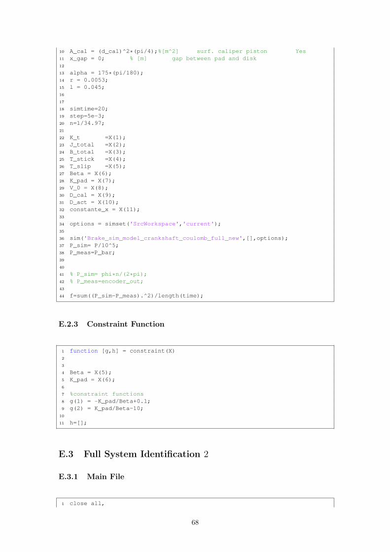
10 A_cal = (d_cal)^2*(pi/4);%[m^2] surf. caliper piston Yes11 x_gap = 0; % [m] gap between pad and disk12

13 alpha = 175*(pi/180);14 r = 0.0053;15 l = 0.045;16

17

18 simtime=20;19 step=5e-3;20 n=1/34.97;21

22 K_t =X(1);23 J_total =X(2);24 B_total =X(3);25 T_stick =X(4);26 T_slip =X(5);27 Beta = X(6);28 K_pad = X(7);29 V_0 = X(8);30 D_cal = X(9);31 D_act = X(10);32 constante_x = X(11);33

34 options = simset('SrcWorkspace','current');35

36 sim('Brake_sim_model_crankshaft_coulomb_full_new',[],options);37 P_sim= P/10^5;38 P_meas=P_bar;39

40

41 % P_sim= phi*n/(2*pi);42 % P_meas=encoder_out;43

44 f=sum((P_sim-P_meas).^2)/length(time);

E.2.3 Constraint Function

1 function [g,h] = constraint(X)2

3

4 Beta = X(5);5 K_pad = X(6);6

7 %constraint functions8 g(1) = -K_pad/Beta+0.1;9 g(2) = K_pad/Beta-10;

10

11 h=[];

E.3 Full System Identification 2

E.3.1 Main File

1 close all,

68

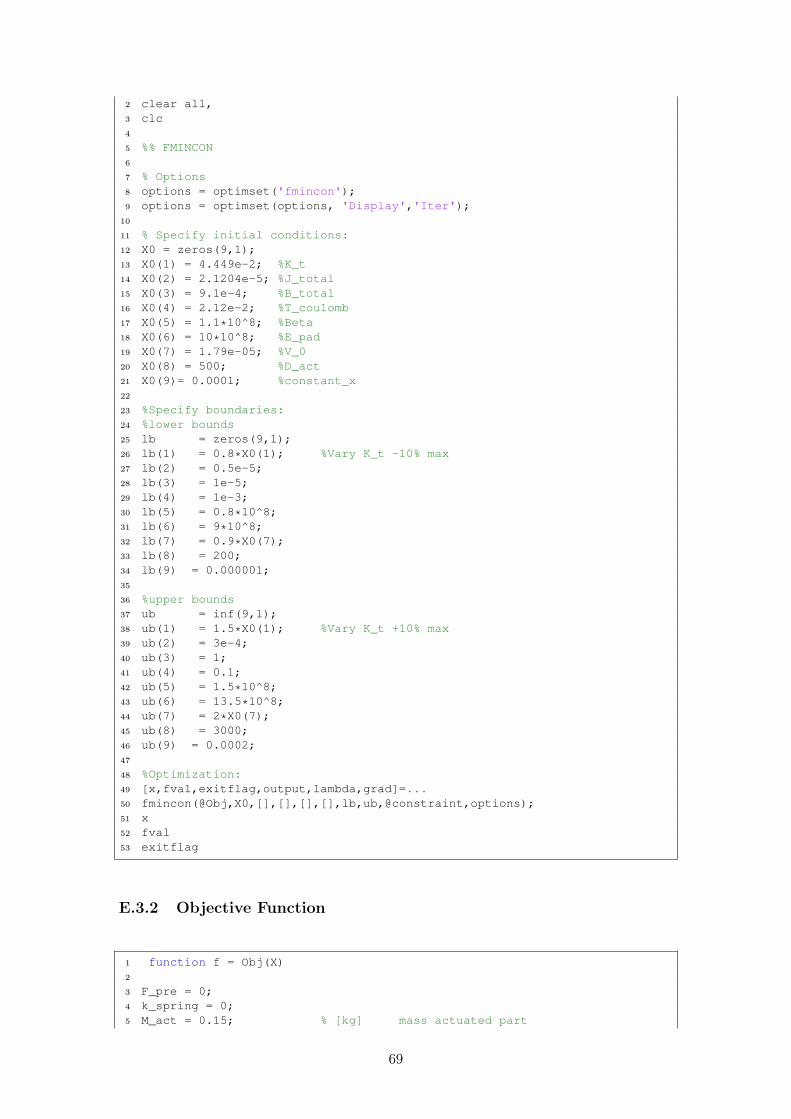
2 clear all,3 clc4

5 %% FMINCON6

7 % Options8 options = optimset('fmincon');9 options = optimset(options, 'Display','Iter');

10

11 % Specify initial conditions:12 X0 = zeros(9,1);13 X0(1) = 4.449e-2; %K_t14 X0(2) = 2.1204e-5; %J_total15 X0(3) = 9.1e-4; %B_total16 X0(4) = 2.12e-2; %T_coulomb17 X0(5) = 1.1*10^8; %Beta18 X0(6) = 10*10^8; %E_pad19 X0(7) = 1.79e-05; %V_020 X0(8) = 500; %D_act21 X0(9)= 0.0001; %constant_x22

23 %Specify boundaries:24 %lower bounds25 lb = zeros(9,1);26 lb(1) = 0.8*X0(1); %Vary K_t -10% max27 lb(2) = 0.5e-5;28 lb(3) = 1e-5;29 lb(4) = 1e-3;30 lb(5) = 0.8*10^8;31 lb(6) = 9*10^8;32 lb(7) = 0.9*X0(7);33 lb(8) = 200;34 lb(9) = 0.000001;35

36 %upper bounds37 ub = inf(9,1);38 ub(1) = 1.5*X0(1); %Vary K_t +10% max39 ub(2) = 3e-4;40 ub(3) = 1;41 ub(4) = 0.1;42 ub(5) = 1.5*10^8;43 ub(6) = 13.5*10^8;44 ub(7) = 2*X0(7);45 ub(8) = 3000;46 ub(9) = 0.0002;47

48 %Optimization:49 [x,fval,exitflag,output,lambda,grad]=...50 fmincon(@Obj,X0,[],[],[],[],lb,ub,@constraint,options);51 x52 fval53 exitflag

E.3.2 Objective Function

1 function f = Obj(X)2

3 F_pre = 0;4 k_spring = 0;5 M_act = 0.15; % [kg] mass actuated part

69

6 M_cal = 0.9; % [kg] mass cal. piston + pad7 d_act = 0.01905; % [m] diam. actuator piston8 A_act = (d_act)^2*(pi/4);%[m^2] surf. actuator piston9 d_cal = 0.0599; % [m] diam. caliper piston

10 A_cal = (d_cal)^2*(pi/4);%[m^2] surf. caliper piston11 x_gap = 0; % [m] gap between pad and disk12 Apad = 0.0011; % [m^2] surface brake pad13 tpad = 0.011;14 alpha = 175*(pi/180);15 r = 0.0053;16 l = 0.045;17 simtime=20;18 step=5e-3;19 n=1/34.97;20

21 K_t =X(1);22 J_total =X(2);23 B_total =X(3);24 T_coulomb =X(4);25 Beta = X(5);26 Epad = X(6);27 K_pad = 2*Epad*Apad/tpad;28 V_0 = X(7);29 D_act = X(8);30 constante_x = X(9);31

32 options = simset('SrcWorkspace','current');33

34 sim('Brake_sim_model_crankshaft_coulomb',[],options);35 P_sim= P/10^5;36 P_meas=P_bar;37

38 f=sum((P_sim-P_meas).^2)/length(time);

E.3.3 Constraint Function

1 function [g,h] = constraint(X)2

3 Beta = X(5);4 E_pad = X(6);5

6 %constraint functions7 g(1) = -E_pad/Beta+0.1;8 g(2) = E_pad/Beta-10;9

10 h=[];

70