Embed Size (px)
Citation preview

Design and Control of Integrated Systems for Hydrogen
Production and Power Generation
A DISSERTATION
SUBMITTED TO THE FACULTY OF THE GRADUATE SCHOOL
OF THE UNIVERSITY OF MINNESOTA
BY
Dimitrios Georgis
IN PARTIAL FULFILLMENT OF THE REQUIREMENTS
FOR THE DEGREE OF
Doctor of Philosophy
Advised by Prodromos Daoutidis
November 2013

c© Dimitrios Georgis 2013
ALL RIGHTS RESERVED

Acknowledgments
During my graduate studies at the University of Minnesota I had the opportunity to
meet, interact and work with amazing people who have contributed significantly towards
my PhD completion. I would like to express my deepest gratitude and appreciation to
all these people, therefore, allow me to mention some of them.
First of all, I would like to thank my advisor Professor Prodromos Daoutidis for
his constant support during my graduate studies. His widespread knowledge and skills
motivated me to pursue a PhD in Process Systems Engineering. Furthermore, I would
like to thank Professors Jeffrey Derby, William Smyrl and Mihailo Jovanovic for being
part of my PhD committee.
Many thanks to Professor Ali Almansoori for the great collaboration that we had
during the ADMIRE project. Moreover, I would like to express my appreciation to all
faculty at Petroleum Institute in Abu Dhabi for their hospitality during my visit.
It was a great pleasure working with exceptional colleagues. I would like to thank
Dr. Sujit Jogwar, Dr. Ana Torres Rippa, Dr. Srinivas Rangaranjan, Dr. Alex Marvin,
Seongmin Heo, Dr. Fernando Lima, Dr. Milana Trifkovic, Adam Kelloway, Abdulla
i

ii
Malek, Nahla Al Amoodi, Michael Zachar, Mustafa Caglayan and Udit Gupta for the
amazing moments we had as a group. In addition to this, I feel the need to thank some
former group members of Professor Kumar’s group (Dr. Scott Roberts, Dr. Shawn
Dodds and Dr. Eric Vandre) with whom we shared the same office during the first
years. Furthermore, I would like to thank all the employees in the department for their
valuable service. Specifically I am grateful to Julie Prince who was always willing to
help and assist me. Moreover, I have to mention that I am grateful to our department’s
IT team for their important services and fast responses to any questions I had during
my PhD.
Many thanks to all the members of Hellenic Student Association (HSA) and the
entire Greek community for all the beautiful moments and the nice events. Especially,
I am more than grateful to all my friends for all the beautiful moments we had in Min-
neapolis; thus, making my life here in Minneapolis pleasant, and full of great memories.
Last but not least, I would like to express my appreciation and gratitude to my
parents, my brother, my fiancee and my entire family for their unstoppable support,
love and faith in everything I have done in my life. I firmly believe that without their
support it would be very difficult for me to achieve my goals.

iii
to my family
Abstract
Growing concerns on CO2 emissions have led to the development of highly efficient power
plants. Options for increased energy efficiencies include alternative energy conversion
pathways, energy integration and process intensification. Solid oxide fuel cells (SOFC)
constitute a promising alternative for power generation since they convert the chemical
energy electrochemically directly to electricity. Their high operating temperature shows
potential for energy integration with energy intensive units (e.g. steam reforming reac-
tors). Although energy integration is an essential tool for increased efficiencies, it leads
to highly complex process schemes with rich dynamic behavior, which are challenging
to control. Furthermore, the use of process intensification for increased energy efficiency
imposes an additional control challenge.
This dissertation identifies and proposes solutions on design, operational and con-
trol challenges of integrated systems for hydrogen production and power generation.
Initially, a study on energy integrated SOFC systems is presented. Design alternatives
are identified, control strategies are proposed for each alternative and their validity is
evaluated under different operational scenarios. The operational range of the proposed
iv
v
control strategies is also analyzed. Next, thermal management of water gas shift mem-
brane reactors, which are a typical application of process intensification, is considered.
Design and operational objectives are identified and a control strategy is proposed em-
ploying advanced control algorithms. The performance of the proposed control strategy
is evaluated and compared with classical control strategies. Finally SOFC systems for
combined heat and power applications are considered. Multiple recycle loops are placed
to increase design flexibility. Different operational objectives are identified and a nonlin-
ear optimization problem is formulated. Optimal designs are obtained and their features
are discussed and compared.
The results of the dissertation provide a deeper understanding on the design, oper-
ational and control challenges of the above systems and can potentially guide further
commercialization efforts. In addition to this, the results can be generalized and used for
applications from the transportation and residential sector to large–scale power plants.

Contents
Acknowledgments i
Abstract iv
Table of Contents vi
List of Tables ix
List of Figures xi
1 Introduction 1
1.1 Hydrogen: towards carbon–free power generation . . . . . . . . . . . . . 3
1.2 Fuel Cells: an alternative energy conversion unit . . . . . . . . . . . . . 4
1.3 Process intensification: re–engineering process energy systems . . . . . . 7
1.4 Combined Heat and Power Systems: transforming the energy market . . 9
1.5 Thesis outline . . . . . . . . . . . . . . . . . . . . . . . . . . . . . . . . . 10
vi
CONTENTS vii
2 Solid Oxide Fuel Cells 12
2.1 Basic features and fundamental operation . . . . . . . . . . . . . . . . . 13
2.2 SOFC stack design configurations . . . . . . . . . . . . . . . . . . . . . . 15
2.3 Fuel flexibility . . . . . . . . . . . . . . . . . . . . . . . . . . . . . . . . . 17
3 Energy Integrated Solid Oxide Fuel Cell Systems: Design and Control
Analysis 19
3.1 Introduction . . . . . . . . . . . . . . . . . . . . . . . . . . . . . . . . . . 20
3.2 Integration of SOFC and external steam reformer . . . . . . . . . . . . . 22
3.2.1 SOFC Mathematical Model . . . . . . . . . . . . . . . . . . . . . 22
3.2.2 SR Mathematical Model . . . . . . . . . . . . . . . . . . . . . . . 25
3.3 Steady state analysis . . . . . . . . . . . . . . . . . . . . . . . . . . . . . 26
3.3.1 Solid oxide fuel cell . . . . . . . . . . . . . . . . . . . . . . . . . . 27
3.3.2 Methane Steam reformer . . . . . . . . . . . . . . . . . . . . . . 27
3.4 Energy integration . . . . . . . . . . . . . . . . . . . . . . . . . . . . . . 30
3.5 Open-loop analysis . . . . . . . . . . . . . . . . . . . . . . . . . . . . . . 33
3.5.1 Small step increase in the current . . . . . . . . . . . . . . . . . . 34
3.5.2 Large step increase in the current . . . . . . . . . . . . . . . . . . 38
3.6 Control design . . . . . . . . . . . . . . . . . . . . . . . . . . . . . . . . 40
3.6.1 Closed-loop analysis . . . . . . . . . . . . . . . . . . . . . . . . . 40
3.6.2 Closed-loop simulations . . . . . . . . . . . . . . . . . . . . . . . 42
3.7 Sensitivity analysis . . . . . . . . . . . . . . . . . . . . . . . . . . . . . . 51
3.7.1 Impact of steam reformer design parameters on steady state design 51
3.7.2 Impact of steam reformer design parameters on open–loop behavior 55
3.7.3 Impact of steam reformer design parameters on closed–loop behavior 58
3.8 Discussion . . . . . . . . . . . . . . . . . . . . . . . . . . . . . . . . . . . 60

CONTENTS viii
4 Thermal management of Water Gas Shift Membrane Reactors for si-
multaneous hydrogen production and carbon capture 65
4.1 Introduction . . . . . . . . . . . . . . . . . . . . . . . . . . . . . . . . . . 66
4.2 Background . . . . . . . . . . . . . . . . . . . . . . . . . . . . . . . . . . 68
4.3 Mathematical model . . . . . . . . . . . . . . . . . . . . . . . . . . . . . 73
4.4 Open–loop simulations . . . . . . . . . . . . . . . . . . . . . . . . . . . . 77
4.5 Controller design and closed–loop simulations . . . . . . . . . . . . . . . 81
4.5.1 Nonlinear controller design . . . . . . . . . . . . . . . . . . . . . 81
4.5.2 Disturbance rejection . . . . . . . . . . . . . . . . . . . . . . . . 84
4.5.3 Set point tracking . . . . . . . . . . . . . . . . . . . . . . . . . . 85
5 Optimal Designs in Combined Heat and Power Solid Oxide Fuel Cell
Systems 87
5.1 Introduction . . . . . . . . . . . . . . . . . . . . . . . . . . . . . . . . . . 88
5.2 Description of the CHP SOFC system . . . . . . . . . . . . . . . . . . . 89
5.3 Mathematical Problem Formulation . . . . . . . . . . . . . . . . . . . . 91
5.3.1 Mathematical models . . . . . . . . . . . . . . . . . . . . . . . . 91
5.3.2 Optimization problem formulation . . . . . . . . . . . . . . . . . 93
5.4 Simulations . . . . . . . . . . . . . . . . . . . . . . . . . . . . . . . . . . 94
5.4.1 Base case study . . . . . . . . . . . . . . . . . . . . . . . . . . . . 94
5.4.2 Case study 1: Optimal design for maximized electrical efficiency 94
5.4.3 Case study 2: Maximizing the heat–to–power ratio . . . . . . . . 98
5.4.4 Comparison of SOFC temperature distribution . . . . . . . . . . 101
6 Summary and Future Directions 104
Bibliography 107

List of Tables
1.1 Main characteristics of different types of fuel cells [1, 2] . . . . . . . . . 5
3.1 General parameters . . . . . . . . . . . . . . . . . . . . . . . . . . . . . . 33
3.2 Stream composition at the outlet of each major process . . . . . . . . . 33
3.3 Physical properties of each component . . . . . . . . . . . . . . . . . . . 34
3.4 UA values for heat exchangers and steam reformer . . . . . . . . . . . . 34
3.5 MCp values used in the case study . . . . . . . . . . . . . . . . . . . . . 36
3.6 Detailed parameters used in the case study . . . . . . . . . . . . . . . . 36
3.7 Stream temperatures for each configuration . . . . . . . . . . . . . . . . 37
3.8 Controller parameters for both configurations (K: controller gain, τI :
integral time constant) . . . . . . . . . . . . . . . . . . . . . . . . . . . . 41
3.9 Steady state characteristics for different S/C ratios . . . . . . . . . . . . 55
3.10 Comparison of the two configurations . . . . . . . . . . . . . . . . . . . 58
4.1 Composition of syngas and pre–shifted streams . . . . . . . . . . . . . . 78
ix

LIST OF TABLES x
4.2 Inlet Conditions used in simulations . . . . . . . . . . . . . . . . . . . . 79
4.3 Parameters used in simulations . . . . . . . . . . . . . . . . . . . . . . . 79
5.1 Operating conditions for base case scenario . . . . . . . . . . . . . . . . 94
5.2 Case study 1: optimal values for the decision variables . . . . . . . . . . 98
5.3 Case study 2: optimal values for the decision variables . . . . . . . . . . 100

List of Figures
1.1 Plant efficiencies for coal and natural gas–fired (conventional and inte-
grated with CO2 capture units) power plants (adopted from DOE–NETL
Report [3]) . . . . . . . . . . . . . . . . . . . . . . . . . . . . . . . . . . 2
1.2 An illustration of process intensification in high–purity hydrogen gener-
ation unit. . . . . . . . . . . . . . . . . . . . . . . . . . . . . . . . . . . . 8
2.1 Basic structure of a SOFC single cell . . . . . . . . . . . . . . . . . . . . 14
2.2 Planar SOFC configuration (adopted from [4]) . . . . . . . . . . . . . . 16
2.3 Tubular SOFC configuration (adopted from [5]) . . . . . . . . . . . . . . 16
3.1 Generic design structure of the SOFC energy system . . . . . . . . . . . 22
3.2 SOFC steady states of the voltage, power and temperature as a function
of the current. . . . . . . . . . . . . . . . . . . . . . . . . . . . . . . . . . 28
3.3 Steam reformer methane conversion at different S/C ratios and mole frac-
tion steady states as a function of the reformer temperature. . . . . . . 29
xi

LIST OF FIGURES xii
3.4 Energy integrated SOFC system - Configuration 1 . . . . . . . . . . . . 31
3.5 Energy integrated SOFC system - Configuration 2 . . . . . . . . . . . . 32
3.6 Open-loop simulation under a small step in the current from 60.3 A to
62 A . . . . . . . . . . . . . . . . . . . . . . . . . . . . . . . . . . . . . . 35
3.7 Open-loop simulation under a large step in the current from 60.3 A to 70 A 39
3.8 Optional caption for list of figures . . . . . . . . . . . . . . . . . . . . . 44
3.9 Closed-loop responses for both configurations under a current step in-
crease from 60.3 A to 62 A. . . . . . . . . . . . . . . . . . . . . . . . . . 45
3.10 Closed-loop responses for both configurations under a current step in-
crease from 60.3 A to 70 A . . . . . . . . . . . . . . . . . . . . . . . . . 46
3.11 Closed-loop responses for both configurations under a current step in-
crease from 60.3 A to 70 A . . . . . . . . . . . . . . . . . . . . . . . . . 47
3.12 Current changes imposed to analyze the operating range for both config-
urations . . . . . . . . . . . . . . . . . . . . . . . . . . . . . . . . . . . . 48
3.13 Closed-loop responses under the current step changes considered in this
analysis (Figure 3.12) . . . . . . . . . . . . . . . . . . . . . . . . . . . . 49
3.14 Closed-loop responses under the current step changes considered in this
analysis (Figure 3.12) . . . . . . . . . . . . . . . . . . . . . . . . . . . . 50
3.15 Steady states of hydrogen mole fraction as a function of the operating
temperature and S/C ratio . . . . . . . . . . . . . . . . . . . . . . . . . 52
3.16 Projection of hydrogen mole fraction steady states as a function of the
operating temperature at different S/C ratios . . . . . . . . . . . . . . . 53
3.17 Steady states of methane conversion as a function of the operating tem-
perature and S/C ratio . . . . . . . . . . . . . . . . . . . . . . . . . . . . 54
3.18 Open–loop responses under a small step in the current . . . . . . . . . . 56
3.19 Open-loop behavior under a large step in the current . . . . . . . . . . . 57

LIST OF FIGURES xiii
3.20 Closed–loop behavior under a large step in the current . . . . . . . . . . 59
4.1 Conventional process configuration for high and low temperature packed–
bed WGS reactors including carbon capture . . . . . . . . . . . . . . . . 67
4.2 Different designs for a membrane reactor: (a) reaction takes place in the
tube with the membrane placed at its outer wall (b) reaction takes place
in the shell and membrane placed at the outer wall of the permeation zone 69
4.3 Thermal management strategy considered in previous work [6] . . . . . 71
4.4 Thermal management strategy considered in this work . . . . . . . . . . 72
4.5 Distributed cooling zone placement for increased heat removal from the
reaction zone . . . . . . . . . . . . . . . . . . . . . . . . . . . . . . . . . 78
4.6 Reaction zone temperature response at various positions across the axial
dimension . . . . . . . . . . . . . . . . . . . . . . . . . . . . . . . . . . . 80
4.7 Reaction zone temperature distribution at different operating points . . 80
4.8 Closed–loop simulation under a 10% decrease in the pre–shift carbon
monoxide conversion : (a)–(c) controlled variables and (d)–(f) manipu-
lated variables . . . . . . . . . . . . . . . . . . . . . . . . . . . . . . . . 82
4.9 Temperature distribution before and after the imposed disturbance . . . 84
4.10 Comparison between model–based and PI controller for a setpoint change
to 480 K. PI tuning parameters used in this simulation: Kc = 10
(cm3/min/K) and τI = 0.42 (min) (red curves) and Kc = 100
(cm3/min/K) and τI = 0.83 (min) (blue curves) . . . . . . . . . . . . . . 86
5.1 Process configuration for base case scenario . . . . . . . . . . . . . . . . 90
5.2 Species mole fraction distribution in anode and cathode of the SOFC . . 95
5.3 SOFC temperature distribution . . . . . . . . . . . . . . . . . . . . . . . 96
5.4 Optimal design for maximized electrical efficiency . . . . . . . . . . . . . 99

LIST OF FIGURES xiv
5.5 Optimal design for maximized heat–to–power ratio . . . . . . . . . . . . 102
5.6 Comparison of SOFC temperature distribution for each case study . . . 103

CHAPTER 1
Introduction
The extensive use of fossil fuels for power generation for almost a century has evolved
into a severe threat for the environment. Recent reports have provided evidence of
climate change which is mainly attributed to the increasing anthropogenic greenhouse
gas emissions (GHG) in the atmosphere [7, 8]. CO2 is considered the major GHG
emission. Although CO2 emissions have remained almost constant in the last decade
in economically developed countries [8, 9, 10] (mainly due to governmental regulations
on greenhouse gas emissions and tax credits for encouraging investments in renewable
energy resources), the world’s total CO2 emissions exhibit an increasing trend [7, 10]
mainly driven by the emerging economies (e.g. Brazil, India, China). In addition to
this, the projected increase in the world’s population is expected to result in higher
demand for power [11, 12]. It is evident that the CO2 emissions mitigation and the
growing demand for energy constitute major factors of the global energy landscape.
1

1 Introduction 2
Fossil fuel–based power generation accounts for approximately 85% of the produced
energy in US (data refer to 2010 [8]) and 82% of the world’s produced energy [13].
Coal and natural gas are mainly used for electricity generation for residential, commer-
cial or industrial usage, while oil derivatives constitute the main energy carrier in the
transportation sector. Large–scale conventional power plants suffer from relatively low
energy efficiencies as shown in Figure 1.1 since their associated fuel’s chemical energy
undergoes several transformations to finally generate electricity. Furthermore, their cen-
Figure 1.1: Plant efficiencies for coal and natural gas–fired (conventional and integratedwith CO2 capture units) power plants (adopted from DOE–NETL Report [3])
tralized nature requires a high voltage and long transmission grid in order to distribute
the electricity to the consumers. Efficiency losses due to the distribution and transmis-
sion of electricity in the grid (average of 7% efficiency loss for the U.S according to the
U.S Energy Information Administration (EIA) [14]) decrease further the overall energy
efficiency. Large–scale conventional power plants also face efficiency challenges due to

1.1 Hydrogen: towards carbon–free power generation 3
variations in power demand (e.g. part–load operation results in significantly lower ef-
ficiencies [15]), while high energy demands impose further limitations in the electricity
distribution grid. On the other hand, the vast majority of energy in the transportation
sector is generated through internal combustion engines with an efficiency of less than
30% [16]. Therefore, future energy systems for power generation should be more efficient
and flexible (e.g. allowing for decentralized electricity generation) in order to minimize
the environmental impact.
In the following subsections we briefly discuss the main themes of the thesis, pro-
viding a broad motivation for the results to be presented.
1.1 Hydrogen: towards carbon–free power generation
Hydrogen has attracted a lot of attention as a potential fuel alternative in power gen-
eration. Its zero carbon emission during oxidation makes hydrogen an attractive option
for satisfying environmental regulations and mitigating greenhouse gas emissions.
Hydrogen is currently used as a feedstock in the chemical and petrochemical industry
[17]. The majority of hydrogen is produced from fossil fuels (e.g. through steam reform-
ing of hydrocarbons) while a small but increasing percentage of hydrogen production is
based on renewable energy resources (e.g. biomass, solar) [18, 19]. Despite its advan-
tages, its low mass density at atmospheric conditions requires high pressure compression
in order to achieve a proper energy content per unit volume [20]. H2–fed vehicles are a
representative example employing high pressure (e.g. 5000 psi [21]) hydrogen storage in
tanks. In addition to this, given the remote location of the H2 fueling stations and the
lack of a well developed hydrogen infrastructure [22], this option results in high capital
and operational costs. An alternative option involves the in–situ hydrogen production
which eliminates any need for storage or transportation [23, 24, 25].

1.2 Fuel Cells: an alternative energy conversion unit 4
In–situ hydrogen production in energy systems requires an additional process unit to
be integrated with the primary power generation unit which is usually referred to as fuel
processor. Integrated energy systems involving in–situ hydrogen production and power
generation lead to complex process schemes which are challenging to design, operate
and control [24].
1.2 Fuel Cells: an alternative energy conversion unit
Fuel cells are electrochemical devices similar to batteries which, unlike conventional
power systems, convert the chemical energy directly into electricity, thus resulting in
higher energy efficiencies. Fuel cells consist of three major compartments: the anode,
the electrolyte and the cathode. The electrolyte is a proton or ion conductive medium
(liquid or solid). The fuel and the oxidant are fed in the anode and cathode respectively,
where electrochemical reactions take place. In the anode, electrons are released and
travel through an external circuit towards the cathode generating electricity. Heat is
also produced as a byproduct of the electrochemical reactions. The ability of fuel cells
for continuous operation as long as fuel is supplied differentiates them from conventional
batteries and makes them promising alternatives for power generation.
Different types of fuel cells have been developed; these are classified based on their
operating temperature in low, intermediate and high temperature fuel cells. Represen-
tative types of fuel cells for each category include the Polymer Exchange Membrane
(PEM) fuel cells, Phosphoric Acid Fuel Cells (PAFC), Molten Carbonate Fuel Cells
(MCFC) and Solid Oxide Fuel Cells (SOFC). Their main features are illustrated in
Table 1.1, where CHP denotes Combined Heat and Power. Apart from their different
operating temperature, fuel cells exhibit different features in terms of materials selec-
tion, electrolyte conductivity and fuel flexibility. A comparative analysis of the basic

1.2 Fuel Cells: an alternative energy conversion unit 5
Table 1.1: Main characteristics of different types of fuel cells [1, 2]
Fuel Cell PEM PAFC MCFC SOFCOperating
Temperature40–80oC 150–200oC 600–700oC 600–1000oC
ElectrolytePolymericMembrane
PhosphoricAcid
MoltenCarbonates
Ceramics
Applications
PortableTransportation
Distributedgeneration
Distributedgeneration
CHP
StationaryDistributedgeneration
CHP
StationaryDistributedgeneration
CHP
features of PEM and SOFC fuel cells, which are considered to be closer to large–scale
commercialization than the other types of fuel cells, reveals their potential range for
different applications. PEM fuel cells are low temperature fuel cells employing a proton
conductive solid (e.g polymeric membrane) electrolyte, exhibiting high power densities
and quick start up responses. However, their slow kinetics at the cathode results in
elevated capital cost for noble metals (e.g. Pt) in the electrodes [26]. In addition to
this, low temperature PEM fuel cells require high–purity hydrogen as a fuel, since they
are sensitive to fuel impurities (e.g. CO) which can potentially poison the polymeric
membrane resulting in a performance degradation [27]. Apart from the above mentioned
challenges, water management in the cathode is a major issue in low–temperature PEM
fuel cells. To alleviate the above challenges, high temperature (>100oC) PEM fuel cells
have attracted a lot of attention since they have demonstrated a higher tolerance to fuel
impurities, potential for lower capital cost through the use of non–platinum catalyst
and easier water management [28, 29]. Despite their attractive features, high operating
temperatures cause problems related to membrane dehydration and materials degrada-
tion [30, 31]. On the other hand, SOFC fuel cells require expensive ceramic materials in
order to tolerate the high operating temperatures while they exhibit a high fuel flexibil-
ity [27]. Their high fuel flexibility allows their integration with conventional (e.g. coal)
power plants and internal combustion engines as an auxiliary unit [32]. Furthermore,

1.2 Fuel Cells: an alternative energy conversion unit 6
their potential for co–generation of heat and power makes them an attractive option for
CHP applications and promising for energy integration with energy intensive processes
such as steam reformers.
The first application of fuel cells was in the aerospace industry during the mid–
60s and 70s [33]. However, the growing need for highly efficient power generation has
brought them to the forefront of power generation. Several companies have manufac-
tured and commercialized fuel cells for residential and decentralized stand–alone appli-
cations ranging from 5 kW to MW–scale fuel cell modules. Some representative fuel cell
companies include: Ballard (PEM), ClearEdge Power (PEM–PAFC), Fuelcell Energy
(MCFC), Bloomenergy (SOFC) and Siemens Westinghouse (SOFC). In addition to this,
the automotive industry has demonstrated high interest in fuel cells as a potential al-
ternative to internal combustion engines and promising for integration with the existing
technology in hybrid vehicles [34]. Several prototype vehicles have been manufactured
while a small number of commercialized vehicles are available in selected areas around
the world (e.g. South California, Japan)[21]. A complete list with more details on the
technical specifications of different fuel cell vehicles can be found in [21].
Although high temperature (1000oC) SOFC fuel cell systems have been already
commercialized, their high capital cost and limited lifetime has motivated research and
development of intermediate temperature SOFC fuel cell systems. Given the reduced
ionic conductivity of the electrolyte due to the lower operating temperature, different cell
configurations (e.g. anode–supported) have been demonstrated to reduce the electrolyte
resistance and achieve a sufficient power density. Given the SOFC potential for energy
integration, process systems analysis is essential in such integrated energy systems in
order to determine design limitations, operational feasibility and controllability.

1.3 Process intensification: re–engineering process energy systems 7
1.3 Process intensification: re–engineering process energy
systems
Process intensification emerged in the early 80’s, driven by the need for increased process
efficiencies in the chemical industry [35]. According to [36]:
’Any chemical engineering development that leads to a substantially smaller,
cleaner, safer and more energy efficient technology is process intensification’.
Typical examples of processes exhibiting process intensification features include reactive
and hybrid distillation units, reactor heat exchangers, micro–reactors, spinning disk
reactors and rotating bed reactors [35, 37].
Power plants show similarities to conventional chemical plants since both convert
the feedstock to end products through a series of processes. Tighter policies in CO2
emissions and the prospect of zero carbon emissions power generation has motivated
the use of carbon capture technologies. Pre– and post–combustion carbon capture
integration has been proposed using either physical solvent or amine–based absorption
units. Despite their different features, both technologies are energy intensive due to the
large amount of solvent regeneration. As a result the overall efficiency drops as shown
in Figure 1.1.
Membrane reactors have been of great interest since they allow for pre–combustion
process intensification in conventional power plants. A typical example is the high–
purity hydrogen generation unit for carbon–free coal–based power generation. This
unit consists of two packed–bed water gas shift (WGS) reactors where coal–derived
syngas is upgraded to hydrogen and carbon dioxide. CO2 is captured in a conventional
carbon capture unit while the hydrogen is fed to the power generation unit (Figure 1.2).
The use of a WGS membrane reactor allows for simultaneous high–purity hydrogen
production and CO2 capture in a single unit, as shown in Figure 1.2. Membrane reactors
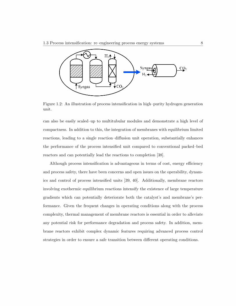
1.3 Process intensification: re–engineering process energy systems 8
Figure 1.2: An illustration of process intensification in high–purity hydrogen generationunit.
can also be easily scaled–up to multitubular modules and demonstrate a high level of
compactness. In addition to this, the integration of membranes with equilibrium limited
reactions, leading to a single reaction–diffusion unit operation, substantially enhances
the performance of the process intensified unit compared to conventional packed–bed
reactors and can potentially lead the reactions to completion [38].
Although process intensification is advantageous in terms of cost, energy efficiency
and process safety, there have been concerns and open issues on the operability, dynam-
ics and control of process intensified units [39, 40]. Additionally, membrane reactors
involving exothermic equilibrium reactions intensify the existence of large temperature
gradients which can potentially deteriorate both the catalyst’s and membrane’s per-
formance. Given the frequent changes in operating conditions along with the process
complexity, thermal management of membrane reactors is essential in order to alleviate
any potential risk for performance degradation and process safety. In addition, mem-
brane reactors exhibit complex dynamic features requiring advanced process control
strategies in order to ensure a safe transition between different operating conditions.

1.4 Combined Heat and Power Systems: transforming the energy market 9
1.4 Combined Heat and Power Systems: transforming the
energy market
In addition to the development of alternative energy conversion units (e.g. fuel cells),
the potential of capturing and transforming the waste heat either into power or useful
heat for heating/cooling purposes has stimulated the development of cogeneration units
also known as combined heat and power (CHP) systems [41]. Given the advantageous
features of SOFC fuel cells for both large–scale and decentralized power plants, SOFC–
based CHP systems are promising for very high overall efficiencies [42, 43] and high grade
heat generation [44, 45]. In addition to this, they offer energy reliability mitigating any
risk for power outages, increase the robustness of the energy infrastructure by decreasing
the load in the transmission grid [46], and limit the investment costs for new expansions
of the transmission network [47]. Thus SOFC–based CHP plants are considered an
attractive option for residential [48] and commercial applications [49].
The total energy consumption in the residential and commercial sectors corresponds
to electricity, heating, and cooling. Current technologies used for heating and cooling
are either gas–fired or electric–fired [50]. Although new, more efficient constructions,
involving better insulation materials, have resulted in a decrease of the demand for
heating/cooling [43], its contribution to the total energy consumption remains significant
(48% in 2009 [51]).
Most of the design analysis in CHP has focused on maximizing the electrical or
overall efficiency. Given the volatile demand for heat and power in residential and
commercial sectors, design flexibility is considered a key factor in CHP plants [52].
To analyze design flexibility, the heat–to–power ratio has emerged as an important
design and operational variable [53]. In addition, the use of material recycles in CHP
plants has been proposed as an option to improve designs and performance [54, 55].

1.5 Thesis outline 10
The effect of recycle ratios has been mainly analyzed using sensitivity analysis [55, 56].
However, introducing more design variables increases the complexity of the CHP plants.
Although sensitivity analysis is usually the first stage of analyzing the impact of one
or more design variables to the plant, optimization tools are essential for determining
the optimal design configuration under different operational modes (e.g. maximum
electrical efficiency and maximum heat to power ratio) given specified operational and
safety–related constraints.
1.5 Thesis outline
The thesis aims to address operational challenges and analyze design alternatives for
highly efficient large–scale and decentralized fuel cell–based power generation. It focuses
mainly on energy systems employing SOFC and process intensification technologies for
simultaneous hydrogen production and carbon capture.
In chapter 2, the SOFC fundamental features and principles of operation are dis-
cussed. Chapter 3 addresses the notion of energy integration in energy systems consist-
ing of a fuel processor and a SOFC. Two energy integrated configurations are analyzed.
A control strategy is proposed for each design alternative and its performance is eval-
uated using linear multi–loop controllers. Furthermore, an overall assessment of the
operability of each design is also performed.
The use of membrane reactors as a process intensification technology for simulta-
neous hydrogen production and pre–combustion carbon capture in energy systems is
considered in Chapter 4. Issues associated with their thermal management are identi-
fied and different control strategies are proposed using model–based controllers.
Chapter 5 discusses process design challenges in SOFC–based CHP plants under
different operational modes. The role of material recycles in SOFC–based CHP plants

1.5 Thesis outline 11
is discussed and an optimization problem is formulated in order to propose optimal
designs for each operational mode. In the last chapter, (Chapter 6) the conclusions of
this thesis are summarized and future directions for continuation of this work are also
briefly mentioned.

CHAPTER 2
Solid Oxide Fuel Cells
Overview: The basic structure and fundamentals on the operation of a Solid
Oxide Fuel Cell single cell are addressed. A brief description on different cell
geometries and configurations is presented. Current technologies allowing
for fuel flexibility are described. Their main features and challenges are also
discussed.
12

2.1 Basic features and fundamental operation 13
2.1 Basic features and fundamental operation
The basic structure of a single SOFC is illustrated in Figure 2.1. The oxidant (e.g. O2)
is fed in the oxidant channel wherein it diffuses to the porous cathode (electrode) and
electrochemically reacts with electrons, supplied through an external electric circuit,
producing oxygen ions:
1
2O2 + 2e− → O2− (2.1)
The produced oxygen ions migrate through the ionic conductive electrolyte to the porous
anode (electrode) participating in the fuel oxidation reaction forming water vapor and
releasing electrons:
H2 + O2− → H2O + 2e− (2.2)
Both reactions take place at the interface of the electrode, the electrolyte and the gas
phase known as triple phase boundary (TPB) point. The continuous movement of
electrons from the anode towards the cathode generates electricity (Figure 2.1) while
heat is released based on the following overall reaction:
H2 +1
2O2 → H2O ∆Ho
298 K = −241.83 kJ/mol
Both the electrodes and the electrolyte are solid materials offering advantages in terms
of design, manufacturing and compactness. The solid nature of the electrolyte coun-
terbalances issues associated with complex electrolyte management and corrosion con-
ditions which typically occur in fuel cells with highly corrosive liquid electrolytes (e.g.
PAFC and MCFC) [33]. In addition, SOFCs show a high tolerance to fuel impurities
and a large fuel flexibility making them promising for integration with a variety of dif-
ferent technologies such as coal/biomass gasification and hydrocarbon steam reforming.

2.1 Basic features and fundamental operation 14
Figure 2.1: Basic structure of a SOFC single cell
The ability of SOFCs to electrochemically oxidize CO:
CO + O2− → CO + 2e− (2.3)
is a characteristic example of improved tolerance to impurities and fuel flexibility. Usu-
ally, CO exists in syngas produced either in gasification [57] or steam reforming units
[58] and has been considered the major poisoning chemical compound in PEM fuel cells.
The SOFC high operating temperature results in low activation energies and high re-
action rates at both electrodes, alleviating the need for expensive noble metals [33, 59]
for the electrodes to promote the reaction rates. Furthermore, internal reforming of
hydrocarbons is considered a unique feature of SOFC, where endothermic steam re-
forming reactions are coupled (either directly or indirectly [60, 61]) with exothermic
electrochemical reactions with potential for higher efficiencies and reduced cooling re-
quirements [62].

2.2 SOFC stack design configurations 15
On the other hand, the SOFCs high operating temperature imposes several chal-
lenges including issues associated with carbon formation though the Boudouard and
cracking reactions:
2CO CO2 + C (2.4)
CH4 2H2 + C (2.5)
leading to anode deactivation [63]. To prevent carbon deposition in the anode electrode,
steam is fed along with fuel at the inlet of the anode. Given the high reaction rates at the
anode, the presence of steam allows the CO to be converted, through the water gas shift
reaction, to CO2 and H2 much faster than its associated electrochemical reaction [33].
Therefore, it is usually assumed that H2 is the only electrochemically active compound
in a SOFC [64, 65, 66]. However, there have been studies in the literature where both CO
and H2 are electrochemically oxidized [67, 68]. In terms of improving the lifetime and
making SOFCs more economically attractive and competitive to other power generation
technologies, substantial efforts have focused on decreasing their operating temperature
(intermediate temperature SOFC), allowing for cheaper materials and reduced thermal
stresses. In the following sections, a discussion of different SOFC designs is presented.
2.2 SOFC stack design configurations
A SOFC stack consists of a number of single cells connected in series in order to scale up
the output power. Two main SOFC stack design configurations have been developed:
the planar (Figure 2.2) and tubular (Figure 2.3). Advantages of planar configuration
include high power densities and reduced fabrication cost while the need for high–
temperature gas tight seals and large thermal stresses constitute common disadvantages.
On the other hand, the tubular configuration eliminates the need for high–temperature

2.2 SOFC stack design configurations 16
Figure 2.2: Planar SOFC configuration (adopted from [4])
gas tight seals and features a improved lifetime. However, the large ohmic losses due to
the tubular geometry lead to lower power densities [69].
Figure 2.3: Tubular SOFC configuration (adopted from [5])
In addition to the different SOFC geometries, different cell configurations are also
available including electrolyte– and electrode–supported configurations. Electrolyte–
supported cell configurations include a thick electrolyte and thin electrodes leading to
low activation and concentration polarizations and high ohmic polarizations. In terms of

2.3 Fuel flexibility 17
electrode–supported SOFCs, anode–supported cell configurations are favored for planar
geometries while the cathode–supported configuration has been used in tubular SOFCs
[70]. The thin electrolyte in the electrode–supported SOFCs allows for a reduced oper-
ating temperature which is beneficial in terms of materials cost and lifetime of the stack
[71]. Based on this unique feature, anode–supported planar SOFCs have attracted a
lot of attention as a promising option for lower operating temperature and high power
densities.
2.3 Fuel flexibility
SOFCs exhibit a wide range of fuel flexibility making them promising candidates for the
entire spectrum of applications for power generation. Typical options for hydrocarbon–
fed SOFCs include: a) internal reforming, b) external reforming and c) direct oxidation
of hydrocarbons.
Internal reforming constitutes a major feature of SOFCs which distinguishes them
from low temperature fuel cells. The option of coupling a highly endothermic reforming
reaction with an exothermic electrochemical reaction results in a process intensified
SOFC unit with increased process efficiencies and no need for an external reforming unit.
As mentioned above, two types of internal reforming are available, direct and indirect
internal reforming. Direct internal reforming involves both physical and thermal contact
of the species within the anode while indirect internal reforming allows only for thermal
contact between the reforming and anode channel. Although indirect internal reforming
is less efficient than direct internal reforming, it provides increased controllability of the
reforming reaction [72].
External reforming is achieved by integrating either steam reforming, partial oxi-
dation or autothermal reforming units upstream to the SOFC. Steam reforming units

2.3 Fuel flexibility 18
lead to high yields of hydrogen however they require reliable thermal management in
order to drive the endothermic reforming reaction [69]. On the other hand, partial
oxidation units exhibit fast transient responses due to the exothermic nature of the
partial oxidation reaction [69]. Oxygen, required for the partial oxidation reaction, is
usually supplied through the use of air. As a result, large amount of nitrogen is fed
to the partial oxidation reactor leading to lower hydrogen concentrations at the outlet
compared to a steam reforming unit. The effect of employing either a partial oxidation
or a steam reforming reactor on a propane–fed SOFC was analyzed in [73]. The study
showed that the nitrogen dilutes the concentration of hydrogen at the anode of the
SOFC leading to a lower operating voltage and hence a lower performance. Autother-
mal steam reformers are process intensified units including both the steam reforming
and the partial oxidation reaction within the same process unit. Autothermal reform-
ing units adopt the advantages of the partial oxidation unit and have a higher yield
of hydrogen compared to the partial oxidation unit [69]. However, the combination of
highly exothermic and highly endothermic reactions exhibit complex dynamic behavior
and requires sophisticated control algorithms for proper thermal management [74].
Direct oxidation of hydrocarbons within the SOFC has attracted a lot of attention as
an alternative to hydrocarbon steam reforming. The operation of SOFCs under direct
electrochemical oxidation is expected to make them more attractive for transportation
and distributed power generation [75]. The operation of direct oxidation SOFCs has
been analyzed for several types of fuels (e.g. methane, ethane, n–butane, diesel) [75, 76,
77, 78]. The option of direct electrochemical oxidation alleviates the need for diluting
fuels with steam and decreases the complexity of the entire SOFC system [79]. Issues
associated with carbon formation at high temperature [78, 77] and poor performance at
low temperatures [77] have motivated a lot of research on alternative anode materials.

CHAPTER 3
Energy Integrated Solid Oxide Fuel Cell Systems: Design and Control
Analysis∗
Overview: Energy integrated SOFC systems are promising for highly ef-
ficient and environmentally friendly power generation. In this chapter, the
design and operation of energy integrated SOFC systems employing an ex-
ternal fuel processor are analyzed. Two design configurations are considered:
one where the hot effluent streams from the fuel cell are used directly for
energy integration, and another where the hot effluent streams are mixed
and combusted in a catalytic burner before the energy integration. A com-
parative evaluation of the two configurations is presented in terms of their
∗Reprinted with permission from Dimitrios Georgis, Sujit S. Jogwar, Ali Almansoori, and ProdromosDaoutidis, Computers & Chemical Engineering 35 (9), 1691–1704 (2011) [24]. Copyright c© 2011 Else-vier Ltd.
Reprinted with permission from Dimitrios Georgis, Sujit S. Jogwar, Ali Almansoori, and Prodro-mos Daoutidis, Proceedings of the 19th Mediterranean Conference on Control & Automation, 576–581(2011) [80]. Copyright c© 2011 IEEE.
19

3.1 Introduction 20
design, open-loop dynamics and their operation under linear multi–loop con-
trollers. In addition, a sensitivity analysis is performed where the effect of
the fuel processor design parameters (steam-to-carbon (S/C) ratio and oper-
ating temperature) on the design, dynamics and control of the entire SOFC
system is analyzed.
3.1 Introduction
Recognizing the need for efficient power generation units, there has been an increasing
interest in developing fuel cell systems for stationary and transportation applications
(see e.g. [81, 82, 83, 84, 85, 86, 87] for excellent overviews on recent developments and
opportunities in modeling and control of fuel cell systems). Given the issues associated
with the storage and transportation of hydrogen, in situ production of hydrogen from
a hydrocarbon fuel, coupled with a H2-fed SOFC, presents a promising approach for
power generation.
Two approaches have been proposed to this end. One of the approaches uses an
external fuel processor [88, 89, 90, 55] to generate a hydrogen-rich stream which is then
fed to the fuel cell while the other approach uses the principle of internal reforming
[55, 91]. In this analysis, we focus on the approach employing an external fuel processor
(e.g. steam reformer) as it offers more opportunities for integration and control design.
A power system consisting of an external steam reformer and a fuel cell exhibits
a lower overall efficiency, since additional energy is required to drive the endothermic
reforming reactions. However, given the SOFC high operating temperature (800 oC-
1000 oC), the hot streams leaving the SOFC show potential for energy integration
by supplying energy to the endothermic reformer, and thereby improving the overall
efficiency. Different integration strategies for SOFC energy systems have been proposed

3.1 Introduction 21
(see e.g. [92] which reviews most of these strategies). These include hybrid integration
strategies with direct thermal coupling [93, 94], indirect thermal coupling [95] as well
as fuel coupling [96], and advanced integration strategies using gas/humid air/steam
turbines [97, 98, 99, 100]. Some of these strategies directly (without mixing the anodic
and cathodic stream) use the hot SOFC effluent for energy recovery (e.g. [101, 102]),
while others use a catalytic burner to further recover energy from the unreacted fuel
and utilize this stream for energy integration (e.g. [93, 90]). While each of these
approaches has obvious advantages/disadvantages in terms of capital and operating
costs, compatibility with downstream processes, and environmental impact, they also
offer different opportunities and challenges in terms of overall integrated system design,
dynamics and control. This is a rather untouched subject in the literature. Motivated by
this, in this chapter we compare (and contrast) these two approaches at the design and
operational stages. The results of this analysis can guide the selection of a particular
approach. To this end, we consider a generic SOFC energy system with an external
methane steam reformer. Energy recovery is achieved by designing a heat exchanger
network (HEN). Through open-loop simulations under imposed step changes in the
current, the dynamic behavior of each of the configurations is analyzed. Linear multi-
loop control strategies are proposed for each case and the operational characteristics are
compared through closed-loop simulations.
The structure of the chapter is as follows. The modeling details for the fuel cell and
the reformer are presented in section 3.2. The selection of operating points for each
of these units based on steady state analysis is presented in section 3.3. The design,
dynamics and control aspects of the energy integrated configurations are analyzed in
sections 3.4, 3.5 and 3.6, respectively. The impact of steam reformer design parameters
on the design and control of the entire energy integrated configuration is addressed in
section 3.7.

3.2 Integration of SOFC and external steam reformer 22
3.2 Integration of SOFC and external steam reformer
A generic SOFC energy system employing an external methane steam reformer (SR) is
shown in Figure 3.1. As the reformer and the fuel cell operate at a high temperature,
Figure 3.1: Generic design structure of the SOFC energy system
three heat transfer units are required to heat the methane steam mixture, fuel cell anode
and cathode inlet streams. Furthermore, energy is required for sustained hydrogen
production in the endothermic steam reformer. In the following subsections, we present
the modeling details for the fuel cell and the reformer which are the major operation
units of the system.
3.2.1 SOFC Mathematical Model
The open-circuit voltage that can be generated by the fuel cell is given by the Nernst
equation:
EOCV = Eo(TFC) +RTFC
2Fln
(pFC,H2 ·p0.5FC,O2
pFC,H2O
)(3.1)

3.2 Integration of SOFC and external steam reformer 23
where Eo(TFC) is the temperature dependent standard potential [33], pi denotes the
partial pressures of each species i at the anode, TFC is the temperature of the fuel cell
and F is the Faraday constant. However, when connected in a circuit, the output voltage
of the fuel cell decreases due to the existence of irreversible losses (called polarizations).
The output voltage of the fuel cell delivered to the load is given by the following equation:
VFC = EOCV − ηact − ηohm − ηconc (3.2)
where ηact, ηohm, ηconc represent the activation, ohmic and concentration polarizations
respectively. Activation polarization is described as the energy barrier that should be
overcome by the reacting species. It is calculated using the Bulter-Volmer equation
[103]:
I = Io ·{exp
(αnFηactRTFC
)− exp
(−(1− α)
nFηactRTFC
)}(3.3)
where Io is the apparent exchange current (calculated following [104]) and α the transfer
coefficient. The voltage drop due to the resistance in the flow of electrons and ions can
be described by the ohmic polarization which is determined by Ohm’s law as shown
below:
ηohm = I·(Ran +Rel +Rca +Rint) (3.4)
whereRi is the resistance of each compartment (calculated from [105]) and the subscripts
(an, el, ca, int) refer to the anode, the electrolyte, the cathode and the interconnector.
Moreover, concentration polarization represents the voltage drop due to the concentra-
tion gradients between the bulk gases and the triple phase boundary point, the interface
between the electrolyte and the electrode where the electrochemical reactions occur. It

3.2 Integration of SOFC and external steam reformer 24
is calculated from the following equation:
ηconc =RTFC
2Fln
(IL
IL − I
)(3.5)
where IL is the limiting current in the fuel cell. The output voltage and the power for
the entire SOFC stack are given below:
V = N ·VFC (3.6)
P = I·V (3.7)
where N is the number of individual cells in the stack.
We now move to the material and energy balance equations for the fuel cell. The
objective of this study is to analyze the system-wide characteristics of energy inte-
grated SOFC systems. Recent studies have shown, through experimental validation,
that lumped parameter models are sufficiently accurate for such systems-level analysis
and control [106]. Numerous other papers also employ lumped parameter models for
analysis and control of SOFC systems (see e.g. [98, 88, 107]). Therefore, we have used
such a lumped parameter model to describe the dynamics of the fuel cell. It is assumed
that there is no interaction between each individual cell. Therefore, the inlet anode and
cathode flows are split into N streams. In addition, the model assumes constant pres-
sure and physical properties, ideal gas behavior and adiabatic operation. The species
and energy balances take then the following form:
dnFC,H2
dt= nFC,H2,in − nFC,H2 −
I
2F(3.8)
dnFC,H2O
dt= nFC,H2O,in − nFC,H2O +
I
2F(3.9)
dnFC,O2
dt= nFC,O2,in − nFC,O2 −
I
4F(3.10)
3.2 Integration of SOFC and external steam reformer 25
dTFCdt
=1
ρSOFCCpSOFCVSOFC·(Qfuel,in − Qfuel,out
+ Qair,in − Qair,out − nreactedH2·∆Hrxn
FC − I·VFC) (3.11)
nreactedH2=
I
2F(3.12)
Qi =∑j
nj Cpj (Ti − Tref ) (3.13)
where the subscripts (i) and (j) refer to the corresponding streams and components while
(FC) denotes the fuel cell and Qi represents the enthalpy flow. Eq. (3.12) represents
Faraday’s law.
3.2.2 SR Mathematical Model
A methane steam reformer is used to convert methane into a hydrogen-rich stream.
This is accomplished through the following two catalytic reactions:
Reforming reaction: CH4 +H2O CO + 3H2 ∆Ho298 = 206.10 kJ/mol (3.14)
WGS reaction: CO +H2O CO2 +H2 ∆Ho298 = −41.15 kJ/mol (3.15)
Note that even though the first reaction is endothermic and the second is exothermic,
the net system of reactions is endothermic, requiring external energy input for sustained
hydrogen production. Here, we model the reformer as a well-mixed reactor with a
heating jacket. Assuming constant pressure, constant physical properties and ideal gas
behavior, the species mass balances take the form:
dnSR,CH4
dt= nSR,CH4,in − nSR,CH4 −mcat·r1 (3.16)
dnSR,H2O
dt= nSR,H2O,in − nSR,H2O −mcat· (r1 + r2) (3.17)
3.3 Steady state analysis 26
dnSR,CO2
dt= nSR,CO2,in − nSR,CO2 +mcat·r2 (3.18)
dnSR,COdt
= nSR,CO,in − nSR,CO +mcat· (r1 − r2) (3.19)
dnSR,H2
dt= nSR,H2,in − nSR,H2 +mcat· (3r1 + r2) (3.20)
where mcat is the mass of the catalyst and ri is the rate of each reaction. The reaction
rate expressions are obtained based on a Langmuir-Hinshelwood reaction mechanism as
proposed in [108]. The energy balances for the reactor and the jacket have the following
form:
dTSRdt
=(Qfuel,in − Qfuel,out −mcat (r1∆H
rxn1 + r2∆H
rxn2 ) + UASR∆TLM )
(ερgCpg + (1− ε)ρcatCpcat)VSR(3.21)
dTSR,HOTdt
=
(QSR,HOT,in − QSR,HOT,out − UASR∆TLM
)MCpSR,HOT
(3.22)
where the subscripts (g), (cat) refer to the gas and catalyst properties, VSR is the
volume of the steam refomer, ε is the void fraction, UASR is the product of the overall
heat transfer coefficient and the heat exchange area and ∆TLM is the mean logarithmic
temperature difference.
3.3 Steady state analysis
In what follows, a steady state analysis is performed for the SOFC and the reformer in
order to select the operating points for these units. This will provide a starting point
for the design of the integrated SOFC energy system.
3.3 Steady state analysis 27
3.3.1 Solid oxide fuel cell
The steady state values of the output voltage, output power and the cell temperature
as a function of the current are shown in Figure 3.2. It is desirable to operate the SOFC
close to the highest power production point with high fuel utilization (UF ). The fuel
utilization represents the fraction of the incoming hydrogen that is electrochemically
converted in the fuel cell. We selected the operating point corresponding to a current
of 60.3 A. At this point, the power delivered by the fuel cell is 16.4 kW (99% of the
maximum power), the output voltage is 272 V and the fuel cell temperature is 1162.6
K.
3.3.2 Methane Steam reformer
It is desired to operate the steam reformer at a temperature where a stream rich in
hydrogen is produced with a high methane conversion [98]. We first explored the effect
of the steam-to-carbon (S/C) ratio on methane conversion. Figure 3.3(a) shows the
variation of methane conversion with respect to reformer temperature for various values
of S/C ratios. High S/C values show enhanced methane conversion, however, at the cost
of additional heating load. We selected S/C = 4 for this study. Figure 3.3(b) shows
the steady state profiles for various species at the outlet of reformer as a function of
operating temperature. Note that the hydrogen mole fraction shows a maximum for
a reformer temperature close to 980 K. We selected the operating point to be 932.3
K. For this state, the methane conversion is 92.6% and the reformate gas contains
approximately 49% hydrogen.

3.3 Steady state analysis 28
0 10 20 30 40 50 60 70 800
100
200
300
400N
VF
C (
V)
I (A)
0 10 20 30 40 50 60 70 800
5
10
15
20
P (
kW)
V P
(a)
0 10 20 30 40 50 60 70 80950
1000
1050
1100
1150
1200
1250
1300
1350
1400
1450
I (A)
TF
C (
K)
(b)
Figure 3.2: SOFC steady states of the voltage, power and temperature as a function ofthe current.

3.3 Steady state analysis 29
800 850 900 950 1000 1050 1100 1150 12000.5
0.55
0.6
0.65
0.7
0.75
0.8
0.85
0.9
0.95
1
x CH
4
TSR
(K)
:S/C=2:S/C=3:S/C=4:S/C=5
(a)
800 850 900 950 1000 1050 1100 1150 12000
0.1
0.2
0.3
0.4
0.5
y i
TSR
(K)
:CH4
:H2O
:CO2
:CO:H
2
(b)
Figure 3.3: Steam reformer methane conversion at different S/C ratios and mole fractionsteady states as a function of the reformer temperature.
3.4 Energy integration 30
3.4 Energy integration
The system in Figure 3.1 requires four external energy inputs. On the other hand, the
SOFC exit streams leave at a high temperature thus, showing a potential for energy
integration. Motivated by the previously proposed integration strategies [101, 102,
90, 93], two integration alternatives were considered: in the first, the hot anodic and
cathodic exit streams from the fuel cell are used directly as two hot streams, while in
the other, the anodic and cathodic streams are mixed together and are combusted in a
catalytic burner to generate a single hot stream.
As a first step in the design of the energy integrated systems, we used pinch analysis
[109]. Pinch analysis indicated that external hot utility is required for the first system
while the second system is self sustaining. Pinch analysis also indicated the absence of a
pinch point for both the cases, thus allowing for a variety of possible design alternatives
[110].
• Design of integrated configuration based on alternative 1 : Most of the existing
configurations [101, 102] following this alternative focus only on the fuel cell and
do not incorporate any fuel processing unit. In this study we incorporated such a
fuel processing unit and we designed the heat exchanger network with the objective
of achieving the minimum external utility predicted by the pinch analysis. The
resulting integrated configuration is depicted in Figure 3.4. The cathode outlet
stream provides energy to the steam reformer (SR) and then it is then split into
two streams. One preheats the air in HE7, while the other supplies energy for
preheating methane in HE4, water in HE1 and steam in HE3. The anode outlet
stream covers the heating requirement of the anode inlet in HE6. Then, it preheats
the fuel mixture to the required reformer inlet temperature in HE5 and then
supplies the required energy for steam generation in HE2. An external hot utility

3.4 Energy integration 31
Figure 3.4: Energy integrated SOFC system - Configuration 1
is supplied to the furnace in order to heat the air to the required temperature.
The resulting energy requirement (see Table 3.1) in this configuration is exactly
the one predicted by the pinch analysis.
• Design of integrated configuration based on alternative 2 : In this case, we used the
integrated configuration proposed in [90] as a basis and achieved further recovery
and recycle of energy, specifically through the addition of heat exchangers (1-3), (5)
and (7) as shown in Figure 3.5. The anodic and cathodic outlet streams are fed to
a catalytic burner, where the complete combustion of methane, carbon monoxide
and unreacted hydrogen takes place. The required air is supplied by the SOFC
cathodic stream. The high temperature stream leaving the burner heats the air in

3.4 Energy integration 32
Figure 3.5: Energy integrated SOFC system - Configuration 2
HE6 and provides energy to the anode inlet stream in HE5. Then, it passes through
the steam reformer (SR) in order to cover its endothermic demand. Leaving the
reformer, the hot stream heats the fuel mixture to the temperature required by the
reformer in HE3 and then preheats the air stream in HE4. Afterwards, it provides
energy for both the preheating of the methane in HE7 and the steam generation
in HE2 and HE1.
Both configurations use seven process-to-process heat exchangers. While the first
configuration uses a furnace (external energy source), the other uses a combustion unit
(internal energy source). Bypasses b2 and b3 are placed to improve the controllability
of the first configuration, while bypasses b1, b2 and b3 are placed in the second config-
uration for the same reason. Tables 3.1 and 3.3-3.6 present the parameters that have
been used for both configurations. Note that the same operating points (as selected in
the previous section) are used for the fuel cell and the reformer. The composition and
the total molar flow rate at the outlet of each major process are tabulated in Table 3.2.

3.5 Open-loop analysis 33
Table 3.1: General parameters
Parameter Value Parameter Value
N 384 PFC (kPa) 101.3V (V) 272 PSR (kPa) 150.0I (A) 60.3 QF (kW) 4.347P (kW) 16.4 xCH4 0.926S/C 4 nSR,in (mol/s) 0.225UF 0.8 nair (mol/s) 2.111
Configuration 1 Configuration 2
β1 0.09 b1 0.10b2 0.10 b2 0.10b3 0.10 b3 0.10
The temperatures at each stream arising from the energy integration are tabulated in
Table 3.7.
Table 3.2: Stream composition at the outlet of each major process
SR SOFC CB
yCH4 0.011 0.011 0yH2O 0.368 0.757 0.116yCO 0.054 0.054 0yCO2 0.081 0.081 0.019yH2 0.486 0.097 0yO2 - 0.184 0.151yN2 - 0.816 0.714ntotal (mol/s) 0.308 - 2.336nan,total (mol/s) - 0.308 -nca,total (mol/s) - 1.840 -
3.5 Open-loop analysis
We next studied the dynamic response of each of these configurations. We considered
a scenario where current changes are imposed which may be caused by power changes.

3.5 Open-loop analysis 34
Table 3.3: Physical properties of each component
Component ρi (kg/m3) Cpi (J/mol/K)
CH4 0.717 58.381H2O (g) 0.804 38.459H2O (l) 1000 75.327CO 1.250 31.374CO2 1.977 49.561H2 0.089 30.236O2 1.429 32.582N2 1.251 31.394
Table 3.4: UA values for heat exchangers and steam reformer
UAi (W/K) Configuration 1 Configuration 2
SR 51.42 67.10HE1 24.45 8.09HE2 49.05 104.80HE3 15.36 11.62HE4 2.31 108.10HE5 4.63 3.23HE6 2.31 58.37HE7 1170 3.91
3.5.1 Small step increase in the current
Figure 3.18 shows the response of key variables for a step in the current from 60.3 A
to 62 A. The increase in current causes an instantaneous increase in the amount of
hydrogen reacted in the fuel cell (Eq. 3.12). This is reflected in the corresponding
increase in the fuel utilization and the decrease in the burner temperature (less fuel
for combustion) for the second configuration. The increased hydrogen consumption
also results in increased fuel cell temperature, however over a longer horizon. Yet,
the impact of the disturbance is different for the two configurations. The rise in the
reformer temperature is much larger for configuration 1 than configuration 2. This

3.5 Open-loop analysis 35
0 20 40 60 80 100925
930
935
940
945
950
955
time (min)
TS
R (
K)
Configuration 1Configuration 2
(a)
0 20 40 60 80 1001160
1165
1170
1175
1180
1185
1190
1195
time (min)
TF
C (
K)
Configuration 1Configuration 2
(b)
0 20 40 60 80 100965
970
975
980
985
990
995
1000
time (min)
TC
A,in
(K
)
Configuration 1Configuration 2
(c)
0 20 40 60 80 1000.8
0.805
0.81
0.815
0.82
0.825
0.83
0.835
time (min)
UF
Configuration 1Configuration 2
(d)
0 20 40 60 80 1001332
1334
1336
1338
1340
1342
1344
time (min)
TC
B (
K)
(e)
Figure 3.6: Open-loop simulation under a small step in the current from 60.3 A to 62 A

3.5 Open-loop analysis 36
Table 3.5: MCp values used in the case study
MCpi (J/K) Configuration 1 Configuration 2
SRH 26.45 36.54F 35.31 -CB - 36.54HE1,HOT 2.61 36.54HE2,HOT 0.19 36.54HE3,HOT 2.61 36.54HE4,HOT 2.61 36.54HE5,HOT 5.84 36.54HE6,HOT 5.84 36.54HE7,HOT 26.46 36.54HE1,COLD 857.89 857.89HE2,COLD 3.52 3.52HE3,COLD 3.52 4.74HE4,COLD 1.30 26.48HE5,COLD 4.74 5.36HE6,COLD 5.36 26.48HE7,COLD 35.31 0.86
Table 3.6: Detailed parameters used in the case study
Parameter Value Parameter Value
L (m) 0.1 VSR (L) 3.3W (m) 0.1 ρcat (kg/m3) 2335A (cm2) 100 ε 0.4ρSOFC (kg/m3) 4200 Cpcat (J/kg/K) 444CpSOFC (J/kg/K) 640 ∆Hrxn
FC (kJ/mol) -241.83τan (mm) 1 ∆Hrxn
1 (kJ/mol) 206.10τel (µm) 8 ∆Hrxn
2 (kJ/mol) -41.15τca (µm) 50 τint (mm) 1
is due to the fact that the inlet temperature for configuration 1 is higher than the
nominal value, while for the second configuration, it is lower than the nominal value.
The responses of the reformer temperature and the cathode inlet temperature show
striking differences between the two configurations. In configuration 1, the increase

3.5 Open-loop analysis 37
Tab
le3.7
:S
trea
mte
mp
erat
ure
sfo
rea
chco
nfi
gura
tion
Con
figu
rati
on
1C
onfi
gura
tion
2
Tem
per
atu
re(K
)T
emp
erat
ure
(K)
Tem
per
ature
(K)
Tem
per
atu
re(K
)
TCH
4,in
298
.0THE5H
1001
.4TCH
4,in
298.
0THE5C
973.
0TH
2O,in
298
.0THE5C
822.
9TH
2O,in
298.
0TSR
932.
3Tair,in
298
.0TSR
932.
3Tair,in
298.
0TSRH
950.
1THE1C
373
.0TSRH
981.
5THE1C
373.
1TSRH,out
963.
8THE1H
308
.2TSRH,out
997.
6THE1H
457.
3TFC
1162
.6THE2C
373
.4TFC
1162
.6THE2C
515.
7THE6H
1092
.9THE2H
383
.0THE6H
1125
.3THE2H
470.
6THE6C
1048
.0THE3C
669
.3THE6C
973.
0THE3C
823.
0THE7H
579.
2THE3H
481
.7THE7H
306.
8THE3H
925.
6THE7C
520.
0THE4C
669
.3THE7C
907.
9THE4C
729.
0TCB,in
1143
.1THE5C,in
669
.3TF
973.
1THE4H
586.
8THE3C,in
516.
9THE4H
831
.2TSRH,in
1143
.1THE5H
1087
.1TCA,in
973.
0TCB
1343
.7

3.5 Open-loop analysis 38
in the fuel cell temperature increases the reformer temperature and the cathode inlet
temperature in the same fashion. In the case of configuration 2, the increased current
triggers opposing forces in the burner (increase the inlet temperature and decrease
the temperature rise) resulting in an inverse response. For the magnitude of current
change considered here, the net effect is the reduction in burner temperature below the
nominal value. This drives similar responses in the reformer temperature and cathode
inlet temperature. Thus configuration 2 is less sensitive to the current disturbance than
configuration 1.
3.5.2 Large step increase in the current
We now subject the system to a large disturbance in current. Figure 3.19 shows the open-
loop response of key variables for a step in the current from 60.3 A to 70 A. The responses
for the first configuration indicate an open-loop instability triggered by the change in the
operating region of the steam reformer. More precisely, the increase in the current causes
an increase in the reformer temperature. This increases the hydrogen production rate
supplying more fuel to the fuel cell. However, when the reformer temperature reaches
to a point beyond the maximum hydrogen production (see Figure 3.3(b)), any further
increase in reformer temperature decreases hydrogen production and hence, reduces the
fuel supply to the cell. This drives the cell towards fuel starvation conditions, resulting
in higher temperatures.
In the case of the second configuration, the system reaches a new steady state with
responses similar to the case of a small current step. However, in this case, the catalytic
burner temperature is higher than the nominal value, resulting in similar higher value in
the reformer temperature. Note that the temperature increase in the steam reformer is
quite small to trigger any instability. This again shows the ability of this configuration
to maintain open-loop stability.

3.5 Open-loop analysis 39
0 20 40 60 80 100900
950
1000
1050
1100
1150
time (min)
TS
R (
K)
Configuration 1Configuration 2
(a)
0 20 40 60 80 100
1200
1250
1300
1350
1400
1450
time (min)
TF
C (
K)
Configuration 1Configuration 2
(b)
0 20 40 60 80 100900
950
1000
1050
1100
1150
1200
1250
1300
1350
1400
time (min)
TC
A,in
(K
)
Configuration 1Configuration 2
(c)
0 20 40 60 80 1000.8
0.82
0.84
0.86
0.88
0.9
0.92
0.94
0.96
0.98
1
time (min)
UF
Configuration 1Configuration 2
(d)
0 20 40 60 80 1001250
1300
1350
1400
time (min)
TC
B (
K)
(e)
Figure 3.7: Open-loop simulation under a large step in the current from 60.3 A to 70 A

3.6 Control design 40
Remark 3.5.1 Both open-loop simulation scenarios discussed above were performed for
an increase in the current drawn from the SOFC. In the case of a decrease in the applied
current, both configurations give stable open-loop responses even for large steps in the
current (plots not included).
3.6 Control design
3.6.1 Closed-loop analysis
In this paper we focus on the control problem only on the chemical side of the SOFC
energy system. As chemical side of a SOFC system we refer to the part of the SOFC sys-
tem which includes only the electrochemical phenomena taking place inside the SOFC,
without including any power conditioning unit after the SOFC. The corresponding con-
trol objectives considered involve:
1. SOFC temperature: The SOFC is an exothermic system. An increase in the SOFC
temperature shows potential for material damages while a decrease drops the
ionic conductivity of the electrolyte. Thus, there is a need to regulate the SOFC
temperature. In this case, the SOFC temperature is controlled by manipulating
the air inlet flow rate via the bypass b2.
2. Reformer temperature: The reformer temperature affects the hydrogen production
and hence, the stability, the performance, and the power production level of the
entire energy system. We therefore control the reformer temperature through the
jacket stream flow rate via the bypass b3.
3. Fuel utilization: High fuel utilization values (> 0.95) lead to fuel starvation which
can damage the anode [90]. Also, low fuel utilization values reflect inefficient

3.6 Control design 41
operation. Motivated by this, fuel utilization is controlled in the system by ma-
nipulating the fuel inlet flow rate (nfuel).
4. Cathode inlet temperature: In order to maintain a desired operating point of the
SOFC (especially the SOFC temperature), the cathode inlet temperature is also
controlled. In the first configuration, it is controlled by manipulating the furnace
heat duty while in the other configuration, it is controlled via the bypass (b1).
Proportional integral (PI) controllers were implemented to realize the above control
strategy. Initially, the Ziegler-Nicholds tuning technique was followed with the ultimate
gain (Ku) and the ultimate period (Pu) obtained through the autotuning (ATV) method
[111]. The controller parameters calculated from the above procedure resulted in ag-
Table 3.8: Controller parameters for both configurations (K: controller gain, τI : integraltime constant)
KFC (K−1) 4 · 10−3 τI,FC (s) 200KSR (K−1) 5 · 10−2 τI,SR (s) 100KUF (mol/s) 1 · 10−2 τI,UF
(s) 10KCa (K−1) 5 · 10−4 τI,Ca (s) 80KF (W/K) 20 τI,F (s) 80
gressive control action leading to unstable closed-loop behavior (plots not included in
the chapter). Therefore, we detuned the controllers to get a smoother and stable closed-
loop response as well as similar settling times. The parameters obtained are presented in
Table 3.8. The same controller parameters were used in both the configurations, except
for the cathode inlet temperature control loop. In this loop, the same time constant
but a different controller gain has been used since the manipulated variable is different
in the two configurations.

3.6 Control design 42
3.6.2 Closed-loop simulations
We compared the closed-loop performance of both configurations under a small and a
large current step increase (similar to the steps applied in the sections 3.5.1 and 3.5.2).
We also identified the operating ranges for each of the configurations. Note that the
operating range here is defined as the range of achievable current for which no bypasses
are saturated.
Small step increase in current
A step change from 60.3 A to 62 A in the current is applied and the evolution of
the controlled variables along with their manipulated variables is presented in Figures
3.8 and 3.9. As the step in the current is applied, hydrogen consumption in the fuel
cell increases, thereby causing an increase in the fuel utilization. The fuel utilization
controller increases the fuel flow into the system, in order to increase the hydrogen
production and hence, to decrease and bring the fuel utilization back to the set point.
The increasing current also causes the SOFC temperature to rise, therefore the SOFC
temperature controller reduces the bypass ratio to reduce the SOFC temperature. The
increase in the fuel inlet flow leads to higher energy demand required by the reformer.
According to this, we expect the controller to decrease the bypass on the reformer
hot stream in order to provide more energy to the reformer. This is the case for the
first configuration. However, the controller corresponding to the second configuration
increases the bypass ratio. This action reveals a surplus of energy in the reformer
jacket-side inlet stream compared to its nominal value. This contrasting behavior comes
from the different types of heating streams used in the reformer jacket. In the first
configuration, the cathode exit stream (consisting of oxygen and nitrogen) supplies the
energy to the reformer. The flow rate of this stream remains almost constant (slight

3.6 Control design 43
decrease in oxygen flow occurs due to electrochemical reactions) during the operation.
Thus the increased heating demand of the reformer causes a decrease in the bypass
ratio b3. On the other hand, the other configuration uses a mixture of anodic and
cathodic streams in the reformer jacket. The flow rate of this stream changes almost
in accordance with the change in the reformer inlet flow. The surplus of energy comes
from the increased burner temperature.
The second configuration exhibits higher overshoots compared to the first configura-
tion. This difference again comes from the different nature of the heating streams used
in the reformer jacket. The cathode exit stream (with controlled temperature) intro-
duces a negligible disturbance into the reformer in the first configuration, as compared
to the burner temperature (with uncontrolled temperature) in the second configuration.
Large step increase in current
In section 3.5.2 we showed that the open-loop response of the first configuration is
driven to instability while the second configuration remains stable under a large step
increase in the current. In this section, we perform a closed-loop simulation of the
above configurations under the same large disturbance (60.3 A to 70 A) and we show
the capability of the proposed control scheme to stabilize the open-loop unstable system.
According to the closed-loop responses (Figures 3.10 and 3.11), the first configuration
remains stable under the imposed large disturbance. Stability is achieved since the
reformer temperature controller keeps the operating temperature away from the the
maximum hydrogen production point (see Figure 3.3(b)). Note that both the SOFC
and reformer bypasses are saturated resulting in small offsets in the SOFC and reformer
temperatures. The second configuration remains stable even if the temperature bypass
is saturated causing an offset in the SOFC temperature.

3.6 Control design 44
020
4060
8010
011
61
1162
1163
1164
1165
1166
1167
1168
time
(min
)
TFC (K)
C
onfig
urat
ion
1C
onfig
urat
ion
2se
t poi
nt
(a)
020
4060
8010
092
9
930
931
932
933
934
935
936
time
(min
)
TSR (K)
C
onfig
urat
ion
1C
onfig
urat
ion
2se
t poi
nt
(b)
020
4060
8010
00.
8
0.80
5
0.81
0.81
5
0.82
0.82
5
time
(min
)
UF
C
onfig
urat
ion
1C
onfig
urat
ion
2se
t poi
nt
(c)
020
4060
8010
00.
04
0.05
0.06
0.07
0.08
0.090.
1
0.11
time
(min
)
b2
C
onfig
urat
ion
1C
onfig
urat
ion
2
(d)
020
4060
8010
00.
04
0.06
0.080.
1
0.12
0.14
0.16
0.180.
2
time
(min
)
b3
C
onfig
urat
ion
1C
onfig
urat
ion
2
(e)
020
4060
8010
00.
224
0.22
5
0.22
6
0.22
7
0.22
8
0.22
9
0.23
0.23
1
0.23
2
0.23
3
time
(hr)
nfuel (mol/s)
C
onfig
urat
ion
1C
onfig
urat
ion
2
(f)
Fig
ure
3.8
:C
lose
d-l
oop
resp
onse
sfo
rb
oth
con
figu
rati
ons
un
der
acu
rren
tst
epin
crea
sefr
om60
.3A
to62
A.

3.6 Control design 45
0 20 40 60 80 100968
970
972
974
976
978
980
982
time (min)
Tca
,in (
K)
Configuration 1Configuration 2set point
(a)
0 20 40 60 80 1004270
4280
4290
4300
4310
4320
4330
4340
4350
4360
time (min)
QE
H (
W)
(b)
0 20 40 60 80 1000.095
0.1
0.105
0.11
0.115
0.12
0.125
time (min)
b 1
(c)
Figure 3.9: Closed-loop responses for both configurations under a current step increasefrom 60.3 A to 62 A.

3.6 Control design 46
020
4060
8010
011
60
1165
1170
1175
1180
1185
1190
1195
1200
time
(min
)
TFC (K)
C
onfig
urat
ion
1C
onfig
urat
ion
2se
t poi
nt
(a)
020
4060
8010
092
4
926
928
930
932
934
936
938
time
(min
)
TSR (K)
C
onfig
urat
ion
1C
onfig
urat
ion
2se
t poi
nt
(b)
020
4060
8010
00.
8
0.82
0.84
0.86
0.880.
9
0.92
time
(min
)
UF
C
onfig
urat
ion
1C
onfig
urat
ion
2se
t poi
nt
(c)
020
4060
8010
0−
0.020
0.02
0.04
0.06
0.080.
1
0.12
time
(min
)
b2
C
onfig
urat
ion
1C
onfig
urat
ion
2
(d)
020
4060
8010
0−
0.050
0.050.
1
0.150.
2
0.250.
3
0.350.
4
time
(min
)
b3
C
onfig
urat
ion
1C
onfig
urat
ion
2
(e)
020
4060
8010
00.
22
0.22
5
0.23
0.23
5
0.24
0.24
5
0.25
0.25
5
0.26
0.26
5
0.27
time
(hr)
nfuel (mol/s)
C
onfig
urat
ion
1C
onfig
urat
ion
2
(f)
Fig
ure
3.1
0:C
lose
d-l
oop
resp
on
ses
for
bot
hco
nfi
gura
tion
su
nd
era
curr
ent
step
incr
ease
from
60.3
Ato
70A

3.6 Control design 47
0 20 40 60 80 100950
960
970
980
990
1000
1010
time (min)
Tca
,in (
K)
Configuration 1Configuration 2set point
(a)
0 20 40 60 80 1003950
4000
4050
4100
4150
4200
4250
4300
4350
4400
4450
time (min)
QE
H (
W)
(b)
0 20 40 60 80 1000.08
0.1
0.12
0.14
0.16
0.18
0.2
0.22
time (min)
b 1
(c)
Figure 3.11: Closed-loop responses for both configurations under a current step increasefrom 60.3 A to 70 A

3.6 Control design 48
Operating range investigation
In this section, we impose positive and negative changes in current (Figure 3.12) in
order to identify the operating range for both the configurations. The controlled and
corresponding manipulated variables are presented in Figures 3.13 and 3.14. The first
configuration shows a broader operating range (I ≤ 66.5 A) compared to the second
configuration (58 A ≤ I < 66.5 A).
0 20 40 60 80 100 120 14058
59
60
61
62
63
64
65
66
67
time (min)
Cur
rent
(A
)
Figure 3.12: Current changes imposed to analyze the operating range for both configu-rations
During the first step increase in the current, the first configuration is very close
to saturation while the second configuration shows a bypass (b2) saturation (Figure
3.13(d)) resulting in an offset in the SOFC temperature. As the current decreases
there is no operational and controllability limitation for the first configuration since
less energy is required, and hence the controllers increase the bypasses. However, in
the second configuration there is a decrease in the reformer bypass (b3), leading to
saturation (Figure 3.13(e)). Note that under saturation conditions the systems remain
operable (but not controllable) showing offsets from the set point.

3.6 Control design 49
020
4060
8010
012
014
011
20
1130
1140
1150
1160
1170
1180
1190
time
(min
)
TFC (K)
C
onfig
urat
ion
1C
onfig
urat
ion
2se
t poi
nt
(a)
020
4060
8010
012
014
091
8
920
922
924
926
928
930
932
934
936
time
(min
)
TSR (K)
C
onfig
urat
ion
1C
onfig
urat
ion
2se
t poi
nt
(b)
020
4060
8010
012
014
00.
7
0.72
0.74
0.76
0.780.
8
0.82
0.84
0.86
0.880.
9
time
(min
)
UF
C
onfig
urat
ion
1C
onfig
urat
ion
2se
t poi
nt
(c)
020
4060
8010
012
014
0−
0.050
0.050.
1
0.150.
2
time
(min
)
b2
C
onfig
urat
ion
1C
onfig
urat
ion
2
(d)
020
4060
8010
012
014
00
0.050.
1
0.150.
2
0.250.
3
0.350.
4
time
(min
)
b3
C
onfig
urat
ion
1C
onfig
urat
ion
2
(e)
020
4060
8010
012
014
00.
215
0.22
0.22
5
0.23
0.23
5
0.24
0.24
5
0.25
time
(hr)
nfuel (mol/s)
C
onfig
urat
ion
1C
onfig
urat
ion
2
(f)
Fig
ure
3.1
3:
Clo
sed
-loop
resp
onse
su
nd
erth
ecu
rren
tst
epch
ange
sco
nsi
der
edin
this
anal
ysi
s(F
igu
re3.
12)

3.6 Control design 50
0 20 40 60 80 100 120 140940
950
960
970
980
990
1000
time (min)
Tca
,in (
K)
Configuration 1Configuration 2set point
(a)
0 20 40 60 80 100 120 1404000
4100
4200
4300
4400
4500
4600
4700
time (min)
QE
H (
W)
(b)
0 20 40 60 80 100 120 1400.06
0.08
0.1
0.12
0.14
0.16
0.18
time (min)
b 1
(c)
Figure 3.14: Closed-loop responses under the current step changes considered in thisanalysis (Figure 3.12)
3.7 Sensitivity analysis 51
3.7 Sensitivity analysis
The design of the external fuel processor is a key parameter in energy integrated SOFC
systems since it affects not only the power generation through the hydrogen produc-
tion, but also the energy integration through the amount of energy required by the
endothermic reaction. Therefore, in this section the impact of the steam reformer de-
sign parameters on the design, operation and control of the entire energy integrated
system is analyzed for configuration 1 (Figure 3.4). The selection of this configuration
is motivated by the interesting dynamic features (e.g. open-loop instability) that it
exhibits.
3.7.1 Impact of steam reformer design parameters on steady state
design
(a) Effect of S/C ratio on the steam reformer performance
The steady state mathematical model representing the steam reformer is numerically
solved for different operating temperatures and S/C ratios. Figure 3.15 depicts the
corresponding steady states of hydrogen mole fraction at different operating tempera-
tures and S/C ratios. The hydrogen mole fraction shows a decreasing trend as the S/C
increases. It should be mentioned that higher S/C ratios also cause a rise in the total
molar flow rate at the outlet of the steam reformer since the reaction equilibrium are
shifted to the right hand side. For all the S/C ratios, the reformate is a stream rich in
hydrogen and hence, a suitable fuel stream for SOFC systems. The effect of the steam
reformer operating temperature on the hydrogen production reveals an interesting be-
havior. The hydrogen mole fraction shows a maximum such that the slope at a lower
temperature than the maximum is higher than that at a higher temperature. This can
be attributed to the interplay between a highly endothermic reaction coupled with a

3.7 Sensitivity analysis 52
Figure 3.15: Steady states of hydrogen mole fraction as a function of the operatingtemperature and S/C ratio
mildly exothermic reaction. According to Figure 3.16, the temperatures for maximum
hydrogen production are approximately 995, 1025 and 1080 K. In the same figure, it can
be noted that the slope of the hydrogen mole fraction after the maximum point decreases
as the S/C ratio decreases. Although hydrogen production shows a maximum point,
methane conversion (shown in Figure 3.17) shows an increasing trend along with both
the operating temperature and the S/C ratio. According to Figure 3.17, the increase
in both the operating temperature and the S/C ratio favors the methane conversion
since both of these parameters shift the reaction equilibrium to the right. In general,
it is desired to operate the steam reformer at an operating point which provides a high
methane conversion [98] and a hydrogen production close to its maximum production
point.

3.7 Sensitivity analysis 53
800 850 900 950 1000 1050 1100 1150 12000.3
0.35
0.4
0.45
0.5
0.55
0.6
0.65y H
2
TSR
(K)
:S/C=2:S/C=3:S/C=4
Figure 3.16: Projection of hydrogen mole fraction steady states as a function of theoperating temperature at different S/C ratios
(b) Effect of S/C ratio on the entire SOFC system steady state
In order to provide an adequate level of comparison between the different S/C ratio
cases, we maintain the same fuel utilization (UF ). To achieve a constant fuel utilization
under constant current operation, the hydrogen production at the steam reformer should
be fixed. Therefore, in order to provide a comparison level for the steam reformer, we
chose the operating point for the steam reformer to provide same methane conversions.
As a result, we compared the steady state characteristics under the same fuel utilization
and the same methane conversion. In the following table (Table 3.9), the corresponding
values of various process variables are tabulated.
The results show that with a decrease in the S/C ratio, more fuel and a higher
operating temperature is required in order to maintain the same fuel utilization and
similar methane conversion. Both the higher operating temperature and the increased

3.7 Sensitivity analysis 54
Figure 3.17: Steady states of methane conversion as a function of the operating tem-perature and S/C ratio
fuel flow rate are reflected directly on the amount of energy is required by the steam
reformer (QSR); increasing S/C ratio reduces the required amount of energy to drive
the steam reforming reactions, since high S/C ratios move the equilibrium to the right
as mentioned above.
Although the same fuel utilization and similar methane conversion are maintained
in all the cases, the SOFC operating temperature differs slightly due to the different
mixture compositions at the outlet of the steam reformer. The difference in both the
reformate composition and the SOFC operating temperature leads to a deviation in the
voltage produced by the SOFC.
Although the required energy of the steam reformer is inversely proportional to the
S/C ratio, the total amount of energy (Q) that should be supplied shows an opposite
trend. The main reason for these two opposite phenomena is the rise in the amount of

3.7 Sensitivity analysis 55
Table 3.9: Steady state characteristics for different S/C ratios
S/C = 2 S/C = 3 S/C = 4
nCH4 (mol/s) 0.0494 0.0467 0.0450UF 0.8 0.8 0.8TSR (K) 1005.0 962.0 932.3TFC (K) 1168.3 1163.8 1162.6VFC (V) 0.7265 0.7167 0.7084xCH4 (%) 92.67 92.62 92.61
Q (kW) 2.355 3.196 4.347
QSR (kW) 11.044 10.072 9.432
water. The extra energy which is required for the vaporization of the extra amount of
water dominates and hence, a higher amount of energy is required as external utility.
3.7.2 Impact of steam reformer design parameters on open–loop be-
havior
We now move on to the open-loop simulations under small and large current changes.
It should be noted that the energy integrated SOFC system corresponding to S/C equal
to three and four, can be represented by the same configuration as shown in Figure
3.4. However, for the case of the S/C equal to two, in order to design a heat exchanger
network which will minimize the external utility, the hot effluent streams at the outlet
of the SOFC should be thermally mixed. This requires a more complicated design which
is outside the scope of this analysis.
(a) Open–loop behavior under a small step increase in current
A small step increase in the current is considered and the open-loop simulations for
S/C=3 and S/C=4 are compared. Figure 3.18 depicts the corresponding responses.
As the current increases, more hydrogen is electrochemically oxidized inside the
SOFC leading to a temperature rise (Figure 3.18(b)) and an instantaneous increase in
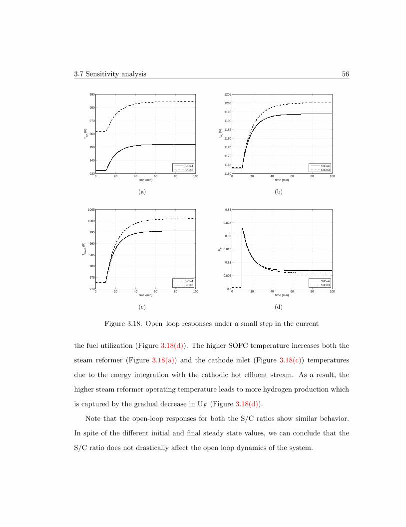
3.7 Sensitivity analysis 56
0 20 40 60 80 100930
940
950
960
970
980
990
time (min)
TS
R (
K)
S/C=4S/C=3
(a)
0 20 40 60 80 1001160
1165
1170
1175
1180
1185
1190
1195
1200
1205
time (min)
TF
C (
K)
S/C=4S/C=3
(b)
0 20 40 60 80 100970
975
980
985
990
995
1000
1005
time (min)
TC
A,in
(K
)
S/C=4S/C=3
(c)
0 20 40 60 80 1000.8
0.805
0.81
0.815
0.82
0.825
0.83
time (min)
UF
S/C=4S/C=3
(d)
Figure 3.18: Open–loop responses under a small step in the current
the fuel utilization (Figure 3.18(d)). The higher SOFC temperature increases both the
steam reformer (Figure 3.18(a)) and the cathode inlet (Figure 3.18(c)) temperatures
due to the energy integration with the cathodic hot effluent stream. As a result, the
higher steam reformer operating temperature leads to more hydrogen production which
is captured by the gradual decrease in UF (Figure 3.18(d)).
Note that the open-loop responses for both the S/C ratios show similar behavior.
In spite of the different initial and final steady state values, we can conclude that the
S/C ratio does not drastically affect the open loop dynamics of the system.

3.7 Sensitivity analysis 57
(b) Open–loop behavior under a large step increase in current
We next analyze the response of the entire SOFC system for a large step increase in the
current. Figure 3.19 depicts the corresponding responses.
0 10 20 30 40 50800
1000
1200
1400
1600
1800
2000
time (min)
TS
R (
K)
S/C=4S/C=3
(a)
0 10 20 30 40 501000
1200
1400
1600
1800
2000
2200
2400
time (min)
TF
C (
K)
S/C=4S/C=3
(b)
0 10 20 30 40 50900
1000
1100
1200
1300
1400
1500
1600
1700
1800
1900
time (min)
TC
A,in
(K
)
S/C=4S/C=3
(c)
0 10 20 30 40 500.8
0.82
0.84
0.86
0.88
0.9
0.92
0.94
0.96
0.98
1
time (min)
UF
S/C=4S/C=3
(d)
Figure 3.19: Open-loop behavior under a large step in the current
The SOFC system is driven to instability in both cases under a large step increase
in the current. The large increase in the current results in a high SOFC temperature
which leads to an increased steam reformer operating temperature. However, the rise
in the steam reformer temperature moves its operating point to the right side of the
maximum hydrogen production point (Figure 3.16) and hence, to a decreasing hydrogen

3.7 Sensitivity analysis 58
production rate. As a result, fuel utilization rises and drives the system to fuel starvation
and instability conditions.
Table 3.10: Comparison of the two configurations
Characteristic Configuration 1 Configuration 2
Design of No pinch - extra No pinch - surplusintegrated system energy is required of energy
Open–loop Stable (small disturbance) Stable (small disturbance)dynamics Unstable (large disturbance) Stable (large disturbance)
Closed–loopSmaller overshoots Larger overshoots
dynamics
OperationalRange
Broader Narrower(bypass saturated (bypass saturated for
for current increase) current increase and decrease)
EnviromentalImpact
No combustionNo mixing of Combustion unit
SOFC outlet streams (potential for NOx)(promising for Mixing of SOFC
further integration outlet streamswith a CO2
capture unit)
3.7.3 Impact of steam reformer design parameters on closed–loop be-
havior
Figure 3.20 depicts the closed-loop responses along with the manipulated variables for
the large step in the current. It can be observed that there are operational limitations

3.7 Sensitivity analysis 59
0 10 20 30 40 50 60 70 80 90 100
930
940
950
960
970
980
time (min)
TS
R (
K)
:S/C=3:S/C=4set point
(a)
0 10 20 30 40 50 60 70 80 90 1001160
1165
1170
1175
1180
1185
time (min)
TF
C (
K)
:S/C=3:S/C=4set point
(b)
0 10 20 30 40 50 60 70 80 90 100−0.02
0
0.02
0.04
0.06
0.08
0.1
0.12
time (min)
b 3
:S/C=3:S/C=4
(c)
0 10 20 30 40 50 60 70 80 90 100−0.02
0
0.02
0.04
0.06
0.08
0.1
0.12
time (min)
b 2
:S/C=3:S/C=4
(d)
0 10 20 30 40 50 60 70 80 90 1000.8
0.82
0.84
0.86
0.88
0.9
0.92
time (min)
UF
:S/C=3:S/C=4set point
(e)
0 10 20 30 40 50 60 70 80 90 100970
972
974
976
978
980
982
984
time (min)
Tca
,in (
K)
:S/C=3:S/C=4set point
(f)
0 10 20 30 40 50 60 70 80 90 1000.175
0.18
0.185
0.19
0.195
0.2
0.205
0.21
0.215
0.22
time (hr)
n fuel
(m
ol/s
)
:S/C=3:S/C=4
(g)
0 10 20 30 40 50 60 70 80 90 100
3
3.5
4
4.5
time (min)
QF (
kW)
:S/C=3:S/C=4
(h)
Figure 3.20: Closed–loop behavior under a large step in the current

3.8 Discussion 60
in both systems due to the saturation of bypasses b2 and b3. It should be mentioned
that these limitations are due to the system design and not due to the controller tuning.
Furthermore, the closed-loop responses reveal a similar behavior in both cases. This
is expected since both systems are designed to operate at the same fuel utilization and
hence, the effect of the SOFC in the entire system is similar in both cases leading to
almost similar closed-loop responses.
3.8 Discussion
Let us now compile the various similarities and contrasting features exhibited by these
two configurations. Table 3.8 summarizes and compares the major characteristics of
these configurations.
• Design of integrated system: Both configurations do not show a pinch point. Ad-
ditional energy is required (and supplied via a furnace) in the first configuration
while energy is available for further integration in the second configuration. Both
configurations use seven process-to-process heat exchangers.
• Open-loop dynamics: Both configurations are stable for small disturbances in cur-
rent. However, the first configuration is driven to instability for a large disturbance
in current, whereas the second configuration remains stable.
• Closed-loop dynamics: The proposed control scheme is capable of stabilizing
the open-loop unstable configuration. Additionally, the first configuration shows
smaller overshoots compared to the second configuration (for the same controller
parameters).
• Operational range: The first configuration has a broader operational range com-
pared to the second configuration. More precisely, the first configuration shows a

3.8 Discussion 61
limitation (due to bypass saturation) at higher current, while the second configu-
ration shows limitations for both the increase and the decrease in the current.
• Environmental impact: The first configuration is less amenable to NOx production
(due to the absence of a combustion unit). Moreover, this configuration looks
promising for further integration with a carbon dioxide capture unit as the anodic
(CH4, H2O, CO2, CO and H2) stream is not mixed with the cathodic (O2 and
N2) stream [89].

3.8 Discussion 62
Nomenclature
Symbol Definition
Capital letters
R Universal gas constant
T Temperature
F Faraday constant
VFC Voltage of single cell
Io Exchange apparent current
I Current
Ri Resistance of each compartment
IL Limiting current
N Number of cells in the SOFC stack
V Output voltage
P Output power
Cpi Heat capacity of component
Vi Volume of each compartment
Pi Operating pressure of each process
∆Hrxni Heat of reaction
Qi Enthalpy flow
U Overall heat transfer coefficient
A Area
∆TLM Logarithmic mean temperature difference
UF Fuel utilization
L Length

3.8 Discussion 63
W Width
Small letters
n Number of transferred electrons
pi Partial pressure of each species
ni Molar flow rate
m Mass
ri Reaction rate
Greek letters
η Number of transferred electrons
α Charge transfer coefficient
ρ Density
ε Void fraction
τ Thickness
Subscripts
FC Fuel cell
OCV Open-circuit voltage
act Activation
ohm Ohmic
conc Concentration
an Anode
el Electrolyte
ca Cathode
int Interconnect

3.8 Discussion 64
fuel Fuel stream
air Air stream
SR Steam reformer
cat Catalyst

CHAPTER 4
Thermal management of Water Gas Shift Membrane Reactors for
simultaneous hydrogen production and carbon capture
Overview: This chapter focuses on the thermal management of a hydrogen-
selective low temperature water gas shift (WGS) membrane reactor for si-
multaneous high purity hydrogen production and carbon capture. A math-
ematical model of the reactor is developed consisting of a set of first–order
hyperbolic PDEs. Open–loop simulations under a step change in the syngas
inlet composition reveal the existence of large temperature gradients along
the reactor. A control strategy is proposed whereby multiple distributed
cooling zones are placed across the reaction zone in order to regulate the
temperature profile. A nonlinear distributed controller is derived and its
performance is evaluated for disturbance rejection and set point tracking
case studies.
65

4.1 Introduction 66
4.1 Introduction
In Chapter 1 the need for highly efficient power plants, along with carbon capture
technologies, was discussed in order to mitigate the environmental impact from the
extensive use of fossil fuels for power generation. Typical examples include the In-
tegrated Gasification Combined Cycle (IGCC) plants for clean coal power generation
[112, 113, 114, 115] and the Combined Heat and Power (CHP) plants integrated with fuel
cells for hydrocarbon-based power generation [116, 117, 24, 118, 119, 120]. Such plants
typically involve the production of hydrogen which generates power either through a
gas turbine or a fuel cell [82].
Coal-, natural gas-, or biomass-derived syngas produces hydrogen through the mod-
erately exothermic and equilibrium limited water-gas-shift (WGS) reaction (3.15). The
equilibrium of the WGS reaction is favored at low temperatures and is unaffected by the
operating pressure. In industrial–scale process units, high pressure syngas is upgraded
to hydrogen and carbon dioxide in two stages [121]. In the first stage, a high temperature
(HT–WGS) packed-bed reactor loaded with iron/chromium (Fe/Cr) catalyst is used to
exploit the fast kinetic rates. The outlet stream of the HT–WGS reactor is cooled and fed
to a low temperature (LT–WGS) packed-bed reactor loaded with copper/zinc (Cu/Zn)
catalyst where the equilibrium is favorable leading to a high CO conversion (see Figure
4.1). The high pressure and concentration of the carbon dioxide at the outlet of the LT–
WGS reactor allows for pre-combustion carbon capture, providing advantages in terms
of sizing and capital cost of the carbon capture unit [122]. Existing mature technologies
available for carbon capture include chemical absorption processes (amine-based and
hot carbonate systems) and physical solvent processes (RectisolTM , SelexolTM ) [123].
Although physical solvent processes are more energy efficient than chemical absorption
processes [122], both technologies require large energy inputs for solvent regeneration.

4.1 Introduction 67
Figure 4.1: Conventional process configuration for high and low temperature packed–bed WGS reactors including carbon capture
An alternative technology, which has attracted a lot of interest [124, 125, 126], allows
for process intensification by replacing the conventional packed-bed WGS reactors and
its associated carbon capture unit with a WGS membrane reactor.
WGS membrane reactors enable simultaneous high–purity hydrogen production and
carbon capture. The combination of production and separation of hydrogen in one unit
can result in substantial improvement in both performance and economics of the entire
plant. However, several studies have demonstrated the risk associated with hot spot
formation which could be detrimental for both the catalyst [121, 127, 128] and the
membrane stability [129, 127, 128].
In this study, we focus on the thermal management of a hydrogen–selective (zeolite-
based) WGS membrane reactor. A dynamic distributed model is developed based on
first principles. A control strategy is proposed and a model–based controller is derived
to regulate the temperature profile of the WGS membrane reactor and suppress thermal
gradients. A case study demonstrates the performance of the proposed control strategy.
In addition, the performance of the model–based controller is compared with that of a
classical PI controller.

4.2 Background 68
The chapter is structured as follows: the next section (Section 4.2) includes a com-
prehensive literature review on modeling and thermal management of WGS membrane
reactors. Results associated with our previous work on modeling, optimization and
control of WGS membrane reactors are also reported. The mathematical model for the
reactor considered is presented in Section 4.3. Open–loop simulations are shown in Sec-
tion 4.4 with the dynamic behavior of the WGS membrane reactor being analyzed under
different operating conditions. The proposed control strategy is presented in Section
4.5 and its performance is evaluated under a case study scenario.
4.2 Background
A membrane reactor typically consists of two concentric cylinders separated by a se-
lective membrane, one of which acts as a reaction zone and the other as a permeation
zone. Two different design configurations have been proposed in the literature[130].
In the first design, the reaction takes place in the tube and the membrane is placed
at the outer wall of the reaction zone [131, 132, 133] (see Figure 4.2(a)), while in the
second design, the reaction zone is in the shell and the membrane placed at the outer
wall of the permeation zone [134, 126] (see Figure 4.2(b)). For both designs, syngas is
fed to the reaction zone where it is upgraded to hydrogen and carbon dioxide in the
presence of steam. Sweep gas (either steam or nitrogen) flows through the permeation
zone either co–currently or counter–currently to the reaction zone flow, allowing for
the recovery of the permeated hydrogen. In terms of performance, it has been shown
that the counter–current flow configuration is more favorable than the corresponding
co–current one [134, 135, 136]. This is attributed to the higher partial pressure differ-
ence of hydrogen developed across the membrane which results in a higher permeation

4.2 Background 69
Figure 4.2: Different designs for a membrane reactor: (a) reaction takes place in thetube with the membrane placed at its outer wall (b) reaction takes place in the shelland membrane placed at the outer wall of the permeation zone
rate. The simultaneous reaction/separation in one process unit shifts the equilibrium-
limited WGS reaction towards higher conversion and increases the residence time of the
reactants across the reaction zone [137], leading to a smaller reactor and less required
mass of catalyst for a given CO conversion. Generally, a hydrogen–selective membrane
is used in WGS membrane reactors. However, the use of a CO2–selective membrane
might be more beneficial when the concentration of CO2 is higher at the inlet of the
membrane reactor compared to hydrogen [131]. Several types of materials for hydrogen–
selective membranes have been proposed [138], with Pd–based membranes considered
suitable when high–purity hydrogen is required. Despite their infinite selectivity for
hydrogen, major drawbacks of Pd–based membranes include high capital cost and hy-
drogen embrittlement [139]. A promising alternative involves the use of zeolite–based
membranes which show the potential for high fluxes, relatively high selectivities and
good hydrothermal stability [136]. More information about different types of hydrogen–
selective membranes and their features can be found in the literature [138, 136].
The permeation rate across the membrane is a function of the partial pressure differ-
ence between the reaction and permeation zone for the permeating component of inter-
est. Therefore, a high operating pressure in the reaction zone enhances the performance
of the reactor. This attribute renders the integration of membrane reactors with coal
gasification or steam reforming (SR) units a promising alternative for pre–combustion
4.2 Background 70
carbon capture. Several studies have analyzed the integration of WGS membrane reac-
tors with either IGCC [140, 141, 142] or fuel cell power plants [143, 144, 145].
In terms of modeling, a large variety of mathematical models of different complex-
ity have been developed. The complexity is determined based on the application and
the scope of the individual study, and can range from steady–state isothermal one-
dimensional to full computational fluid dynamics models. Isothermal operation could
be considered a valid assumption for lab–scale modules, however this assumption is in-
sufficient for larger–scale membrane reactors. Furthermore, it has been demonstrated
that the assumption of isothermal operation leads to an overestimation of the reactor’s
performance [127, 146]. In addition to this, several studies have mentioned the exis-
tence of large temperature gradients which involve potential risks for both the catalyst
and the membrane stability as mentioned above (Section 4.1). Therefore, nonisothermal
models are essential for risk assessment and performance prediction. Different strategies
have been proposed for thermal management of packed–bed reactors exhibiting large
temperature gradients. These alternatives include catalyst dilution with inert pellets
[128, 147, 133], side–stream feed [128, 129, 148] and steam injection [127]. Catalyst di-
lution has been shown to be an effective way to mitigate the hot–spot along the length
of the reactor [147, 127] but unable to suppress it completely and enforce an approxi-
mately uniform temperature profile. Side–stream feed of a reactant is only applicable
in autothermal (e.g. SR) membrane reactors where the flow rate of oxygen controls
the fuel oxidation (e.g. methane) and hence, the heat produced by the oxidation re-
action. As a result, this strategy is suitable only in autothermal membrane reactors
involving highly endothermic reactions (e.g. SR [129] or Methanol Reforming [148])
along with exothermic reactions (e.g. Partial Oxidation). Steam injection constitutes
an alternative option for reducing the temperature in the reaction zone. Although this
strategy is applicable to WGS membrane reactors, it results in a decreased hydrogen

4.2 Background 71
partial pressure and thus, deteriorates the performance of the reactor. In addition to
this, large amounts of steam in the reaction zone could reduce significantly the resi-
dence time in the reaction zone leading to a reduced CO conversion [127]. Furthermore,
large amount of steam injection could also result in increased operating cost. Although
these alternatives could be beneficial in specific applications and operating conditions,
they cannot be generalized as thermal management strategies to any membrane reactor
application. A general control strategy for thermal management of membrane reactors,
which is capable of enforcing an almost uniform temperature profile, would therefore be
valuable.
Figure 4.3: Thermal management strategy considered in previous work [6]
In our previous work [6], we proposed a control strategy for suppressing the hot spots
and ensure the operational feasibility of a high–temperature WGS membrane reactor of
the same design as in Figure 4.2(a). According to this reactor’s design, the membrane
was placed along the entire length of the reaction zone and an inner cooling zone was used
for temperature control (see Figure 4.3). This design however has limited controllability
owing to the single control actuation acting at the entrance of the reactor. Also, there
have been several studies which propose the use of a pre–shift zone with the membrane
reactor [149]. This option results in a lower concentration of reactants at the entrance
of the reaction zone reducing the risk for excessively large temperature gradients at the

4.2 Background 72
Figure 4.4: Thermal management strategy considered in this work
entrance of the reactor. In addition, the placement of a pre–shift zone upstream of the
membrane reactor eliminates any back–permeation of hydrogen at the entrance of the
reactor which occurs during counter–current operation [134]. It also leads to a reduced
membrane area with significant benefits in capital cost. The latter was demonstrated in
our recent study [136] where an optimization problem was formulated based on a one-
dimensional steady–state, isothermal model in order to identify the optimal placement
of catalyst and membrane along the length of the reactor.
Motivated by this, the process configuration considered here consists of a pre–shift
unit followed by a low–temperature membrane reactor. We focus on the thermal man-
agement of the low–temperature WGS membrane reactor with the membrane placed at
the outer wall of the permeation zone (see Figure 4.2(b)). This design allows for dis-
tributed cooling of the reaction zone as in conventional non-adiabatic plug flow reactors
[150] (see Figure 4.4).

4.3 Mathematical model 73
4.3 Mathematical model
A WGS membrane reactor is a classic reaction–diffusion chemical system which includes
flow and reaction in the axial direction and diffusion in the radial direction. Although
two-dimensional models are preferred especially in industrial–scale units in order to
capture the physical phenomena in both directions, they are quite complex and com-
putationally intensive. Furthermore, one-dimensional models have been shown to be
reliable for a overall assessment of the membrane reactor and more computationally
efficient [127]. Especially for small–scale (e.g. lab/pilot) membrane reactors with rela-
tively high length to diameter ratio (L/D) it is expected that the variations in the radial
direction would not be significant.
In this study, we develop a one-dimensional mathematical model for a WGS mem-
brane reactor with a sufficiently large L/D ratio (> 10). In order to maximize the
driving force between the reaction and the permeation zone and hence to enhance the
membrane’s performance, a counter–current flow is considered for the permeation zone.
Steam is used as the sweep gas. Especially in zeolite–based membrane reactors, the
use of steam favors the performance of the reactor since it permeates to the reaction
zone, shifting the equilibrium further towards higher CO conversion. The developed
model includes the following assumptions: a) all gases are considered ideal; b) constant
operating pressure is assumed in all compartments; c) axial dispersion is neglected; d)
uniform catalyst distribution is assumed with a constant porosity along the entire length
of the membrane reactor; and e) velocity dynamics are neglected. According to these,
the mass and energy balances in each compartment are described by a set of first order
hyperbolic PDEs of the following form:

4.3 Mathematical model 74
Species balances in reaction and permeation zones:
∂Cjn+i∂t
= − 1(j+1)
(−∂Fjn+i
∂Vj+ Ji + j·Rwgs
)(4.1)
i = (CO, H2O, CO2, H2, N2)
j =
1, for the reaction zone
0, for the permeation zone
Cjn+i =Fjn+iQj
Ji =
πdtAsQmi (Pi,s − Pi,t) for j=1
πdtAtQmi (Pi,s − Pi,t) for j=0
Rwgs = −νi k(Ts)(P (0.5−Ps/500)s
)(ys,COys,H2O −
ys,CO2ys,H2
Keq(Ts)
)(mcat
Vs
)(4.2)
kwgs(Ts) = 82.2 exp
(−47400
RTs
)Keq(Ts) = exp
(4577.8
Ts− 4.33
)
where C, F , T , V and Q refer to the concentration (mol/m3), molar flowrate (mol/s),
temperature (K), volume (m3) and volumetric flowrate (m3/s) respectively. J cor-
responds to the molar flux across the membrane (mol/m3/s), R is the universal gas
constant (J/mol/K), A is the cross–sectional area of its compartment (m2) and Rwgs
represents the WGS reaction rate (mol/m3/s) with kwgs and Keq its associated kinetic
and equilibrium constants. In the molar flux expression, the variables Qm and Pi re-
fer to the species permeance through the membrane (mol/s/m2/atm) and the species
partial pressures (atm). The subscripts i, n, s, and t denote the species components,
the total number of species components, the reaction zone and the permeation zone.

4.3 Mathematical model 75
The binary parameter j determines the compartment of the membrane reactor. In the
reaction rate expression (equation 4.2), mcat is the mass of the catalyst (kg), νi is the
stoichiometric coefficient for each individual species and the term P (0.5−P/500) refers to
a correction factor for high pressure operating conditions [121].
Energy balances for both reaction and permeation zones:
∂Hj
∂t= − 1(j+1)
−∂(FjMwjHj
)∂Vj
−QdiffAj
− QmemVj
− j·Qcool,zVj
(4.3)
where H, Mw, H denote the enthalpy (J), the mixture molecular weight (kg/mol) and
the mass specific enthalpy (J/kg). The energy flows due to the diffusion and the heat
conduction through the membrane are calculated based on the following equations:
Qdiff =
(n∑i=1
JiMwi
)Hj
Qmem = UmemAt(Ts(z)− Tt(z))
The mass specific enthalpy Hj and enthalpy Hj are evaluated based on the following
equations:
Hj =
n∑i=1
wi
(∆H◦
f,i +
∫ T
Tref
Cpi(T )dT
)
Hj = ρj · Hj
where ∆H◦f,i refers to the standard enthalpy of formation of each component (J/kg),
ρ is the density of the mixture (kg/m3), wi corresponds to the mass fraction of each
component and Cpi(T ) denotes the heat capacity of each component (J/kg/K) as a

4.3 Mathematical model 76
function of the temperature of the following form:
Cpi(T ) = αo,i + α1,iT−1 + α2,iT + α3,i lnT (4.4)
All physical properties are calculated using the IPPFO property package which is in-
cluded in gPROMS Modelbuilder [151].
The distributed cooling zones were modeled assuming well–mixed zones of constant
volume [152] described by a set of ODEs of the following form:
dHcool,z
dt=(F incool,zMwincool,zH
incool,z − Fcool,zMwcool,zHcool,z
)+ Qcool,z (4.5)
where the subscript z refers to each cooling zone and the heat transfer flow associated
with each cooling zone is evaluated using the following equation:
Qcool,z = Ucool,zπds
∫ lf,z
li,z
(Ts(z)− Tcool,z)dz
where li,z and lf,z refer to the initial and final length of each individual cooling zone
respectively.
The following boundary and initial conditions are considered for the reaction and
permeation zones:
Cs,i(0, t) = Cins,i ∀ t, Cs,i(z, 0) = C0s,i ∀ z
Ct,i(L, t) = Cint,i ∀ t, Ct,i(z, 0) = C0t,i ∀ z
Ts(0, t) = T ins ∀ t, Ts(z, 0) = T 0s ∀ z
Tt(0, t) = T int ∀ t, Tt(z, 0) = T 0t ∀ z
For the cooling zone, the mathematical model consists of a set of ODEs, and therefore

4.4 Open–loop simulations 77
only initial conditions are considered:
Tcool,z(0) = T 0cool,z
The developed mathematical model was simulated using the gPROMS Modelbuilder
v3.6 simulation platform using the method of lines to approximate the spatial deriva-
tives. Specifically, the backward finite difference method was used in the reaction and
cooling zones and the forward finite difference method was used in the permeation zone.
A uniform mesh of 100 grid points was used in each compartment. The time integra-
tion of the discretized set of PDEs was performed using the SRADAU solver which is a
variable step numerical method suitable for discretized PDAE systems. All simulations
were performed in a 64–bit Windows 7 CPU equipped with a i7 processor at 2.67 GHz
and 8GB of RAM.
4.4 Open–loop simulations
As mentioned above, a configuration including a pre–shift zone followed by a low tem-
perature membrane reactor has been identified as the optimal design in terms of mem-
brane capital cost [136]. According to this design, a typical syngas stream is fed to the
pre–shift zone where it is assumed that 80% carbon monoxide conversion is achieved.
Afterwards, the pre–shifted stream enters the low temperature WGS membrane reactor
where a high carbon monoxide conversion is achieved (> 98%) and high purity hydrogen
is produced. The composition for both the syngas and the pre–shifted streams is shown
in the following table (Table 4.1).
In order to account for the large amount of heat released at the inlet of the reactor,
instead of placing equi-spaced cooling zones along the reactor (see Figure 4.4) we placed
three cooling zones spaced as follows: 0–0.05 m, 0.05–0.10 m and 0.10–0.20 m (see Figure
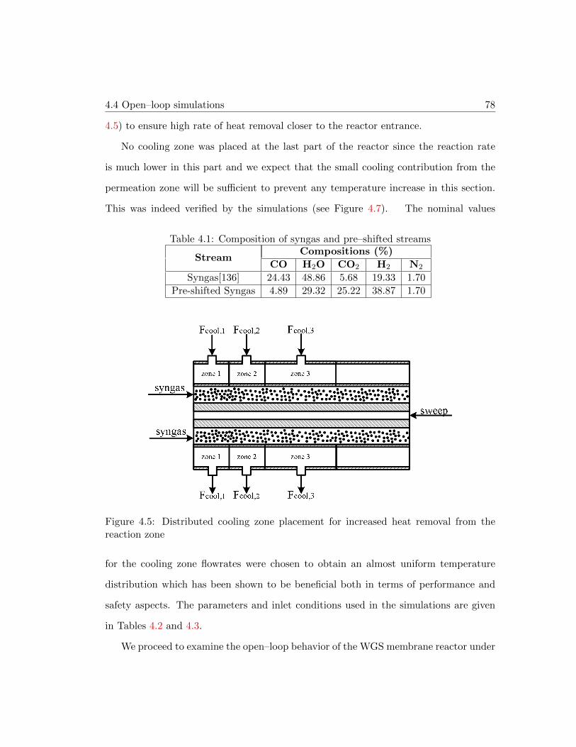
4.4 Open–loop simulations 78
4.5) to ensure high rate of heat removal closer to the reactor entrance.
No cooling zone was placed at the last part of the reactor since the reaction rate
is much lower in this part and we expect that the small cooling contribution from the
permeation zone will be sufficient to prevent any temperature increase in this section.
This was indeed verified by the simulations (see Figure 4.7). The nominal values
Table 4.1: Composition of syngas and pre–shifted streams
StreamCompositions (%)
CO H2O CO2 H2 N2
Syngas[136] 24.43 48.86 5.68 19.33 1.70
Pre-shifted Syngas 4.89 29.32 25.22 38.87 1.70
Figure 4.5: Distributed cooling zone placement for increased heat removal from thereaction zone
for the cooling zone flowrates were chosen to obtain an almost uniform temperature
distribution which has been shown to be beneficial both in terms of performance and
safety aspects. The parameters and inlet conditions used in the simulations are given
in Tables 4.2 and 4.3.
We proceed to examine the open–loop behavior of the WGS membrane reactor under
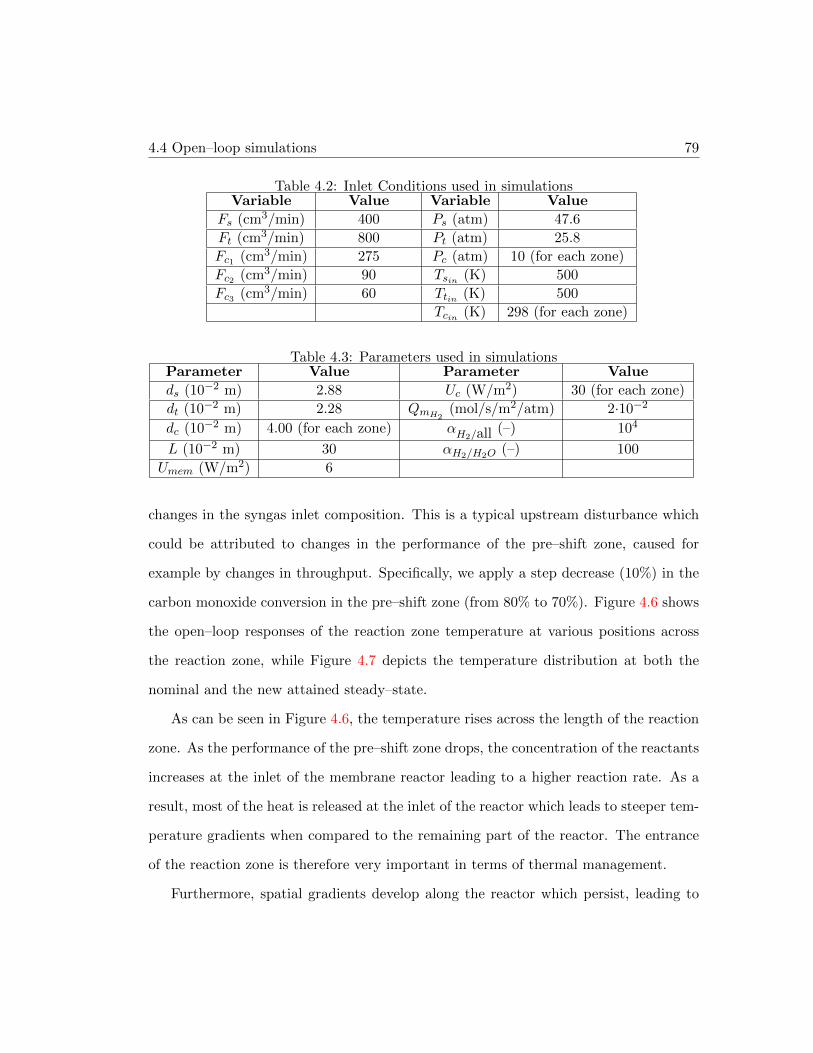
4.4 Open–loop simulations 79
Table 4.2: Inlet Conditions used in simulationsVariable Value Variable Value
Fs (cm3/min) 400 Ps (atm) 47.6
Ft (cm3/min) 800 Pt (atm) 25.8
Fc1 (cm3/min) 275 Pc (atm) 10 (for each zone)
Fc2 (cm3/min) 90 Tsin (K) 500
Fc3 (cm3/min) 60 Ttin (K) 500
Tcin (K) 298 (for each zone)
Table 4.3: Parameters used in simulationsParameter Value Parameter Value
ds (10−2 m) 2.88 Uc (W/m2) 30 (for each zone)
dt (10−2 m) 2.28 QmH2(mol/s/m2/atm) 2·10−2
dc (10−2 m) 4.00 (for each zone) αH2/all (–) 104
L (10−2 m) 30 αH2/H2O (–) 100
Umem (W/m2) 6
changes in the syngas inlet composition. This is a typical upstream disturbance which
could be attributed to changes in the performance of the pre–shift zone, caused for
example by changes in throughput. Specifically, we apply a step decrease (10%) in the
carbon monoxide conversion in the pre–shift zone (from 80% to 70%). Figure 4.6 shows
the open–loop responses of the reaction zone temperature at various positions across
the reaction zone, while Figure 4.7 depicts the temperature distribution at both the
nominal and the new attained steady–state.
As can be seen in Figure 4.6, the temperature rises across the length of the reaction
zone. As the performance of the pre–shift zone drops, the concentration of the reactants
increases at the inlet of the membrane reactor leading to a higher reaction rate. As a
result, most of the heat is released at the inlet of the reactor which leads to steeper tem-
perature gradients when compared to the remaining part of the reactor. The entrance
of the reaction zone is therefore very important in terms of thermal management.
Furthermore, spatial gradients develop along the reactor which persist, leading to

4.4 Open–loop simulations 80
0 5 10 15 20 25 30490
500
510
520
530
Time (min)
Tem
pera
ture
(K
)
:z=0 m:z=0.05 m:z=0.1 m:z=0.15 m:z=0.2 m:z=0.25 m:z=0.3 m
Figure 4.6: Reaction zone temperature response at various positions across the axialdimension
the new steady state with the hot spot shown in Figure 4.7. This open–loop behavior of
the reactor motivates the need for a control strategy able to suppress the temperature
gradients and maintain a uniform temperature profile in the presence of disturbances.
0 0.1 0.2 0.3500
505
510
515
520
525
530
Axial (m)
Tem
pera
ture
(K
)
:t=0 min:t=30 min
Figure 4.7: Reaction zone temperature distribution at different operating points

4.5 Controller design and closed–loop simulations 81
4.5 Controller design and closed–loop simulations
The control of the temperature in the reaction zone is achieved by manipulating the
coolant (air) inlet flowrate. The process configuration considered provides three degrees
of freedom resulting in a multiple–input–multiple–output (MIMO) controller. Given
the distributed nature of the temperature in the reaction zone, we select the average
temperature across a specified section of the reaction zone as the controlled variable:
y(t) =< Tt(z, t) >=1
zf − z0
∫ zf
z0
Tt(z, t)dz (4.6)
where the limits zf and z0 denote to the initial and final position over which the con-
trolled variable is evaluated. Specifically, the controlled variables for the three cooling
sections are:
y1(t) = 20
∫ 0.05
0Tt(z, t)dz
y2(t) = 20
∫ 0.1
0.05Tt(z, t)dz
y3(t) = 10
∫ 0.2
0.1Tt(z, t)dz
4.5.1 Nonlinear controller design
A nonlinear output–feedback controller was derived on the basis of the PDE model
of the reactor following the direct synthesis approach for hyperbolic PDEs in [152].
The controller corresponds to a distributed analogue of the nonlinear inversion–based
geometric control methods for nonlinear ODEs. The characteristic index [152] (which
is the analogue of the relative degree) between the controlled and manipulated inputs

4.5 Controller design and closed–loop simulations 82
05
1015
2025
3050
0
505
510
515
Tim
e (m
in)
Temperature (K)
:CV
(zo
ne 1
)
(a)
05
1015
2025
3050
0
505
510
515
Tim
e (m
in)
Temperature (K)
:CV
(zo
ne 2
)
(b)
05
1015
2025
3050
0
502
504
506
508
510
Tim
e (m
in)
Temperature (K)
:CV
(zo
ne 3
)
(c)
05
1015
2025
30
300
400
500
600
700
Tim
e (m
in)
Q (cm3/min)
:MV
(zo
ne 1
)
(d)
05
1015
2025
30
9095100
105
Tim
e (m
in)
Q (cm3/min)
:MV
(zo
ne 2
)
(e)
05
1015
2025
3060708090100
110
Tim
e (m
in)
Q (cm3/min)
:MV
(zo
ne 3
)
(f)
Fig
ure
4.8
:C
lose
d–lo
op
sim
ula
tion
un
der
a10
%d
ecre
ase
inth
epre
–sh
ift
carb
onm
onox
ide
conve
rsio
n:
(a)–
(c)
con
-tr
oll
edva
riab
les
and
(d)–
(f)
man
ipu
late
dva
riab
les

4.5 Controller design and closed–loop simulations 83
was calculated to be equal to 2. As a result, a decoupled second–order response was
postulated, of the form:
β2,wd2yw(t)
dt2+ β1,w
dyw(t)
dt+ yw(t) = υw(t) (4.7)
where w denotes the control loop, υw refers to a reference input, and β1,w, β2,w are
adjustable parameters.
The process model developed in Section 4.3 can be reformulated in a state–space
representation:
∂x
∂t= A(x)
∂x
∂z+ f(x) + g(x) · u
y = h(x) (4.8)
where x = [x1(z, t) · · ·x15(z, t)]T refers to the state variables, u = [u1(t), u2(t), u3(t)]T
denotes the vector of the manipulated inputs, and y = [y1(t), y2(t), y3(t)]T is the vector of
the controlled variables. A(x)[15×15] and f(x)[15×1], g(x)[15×3], h(x)[3×1] are matrices and
vectors of nonlinear functions. A simplified version of the above process model was used
for the controller synthesis where the heat capacities and the enthalpy of reaction were
assumed constant with respect to temperature and evaluated at the inlet conditions.
In addition, a 10% modeling error was imposed in both the heat transfer coefficients
and the membrane permeation rate. The controller is a combination of a distributed
state–feedback controller derived to induce the postulated closed-loop responses and a
distributed open-loop state–observer.
In order to compensate for the modeling errors, an external proportional–integral

4.5 Controller design and closed–loop simulations 84
(PI) controller was placed around each (υw, yw) loop :
υw(t) = υw,nom(t) +Kwc
(ew(t) +
1
τwI
∫ t
0ew(t)dt
)(4.9)
where: ew(t) = ysp,w(t)− yw(t)
where Kc (dimensionless) and τI (min) refer to the proportional gain and the time
constant of the PI controller respectively.
4.5.2 Disturbance rejection
The controller performance was initially evaluated under the same disturbance scenario
considered in the open–loop simulations. For all simulations the values of the adjustable
parameters were β1,w = 0.83 (min) and β2,w = 0.174 (min2) while the PI controller
parameters were Kc = 0.25 and τI = 0.42 (min), to achieve an overall critically dumped
second–order response with a time constant of 0.83 min (in the absence of disturbances
and modeling errors). Figure 4.8 shows the closed–loop responses for both the controlled
0 0.1 0.2 0.3490
500
510
520
530
Axial (m)
Tem
pera
ture
(K
)
:t=0 min:t=30 min
Figure 4.9: Temperature distribution before and after the imposed disturbance

4.5 Controller design and closed–loop simulations 85
and manipulated variables in each control loop. The controller is successful in regulating
the controlled variables at their set points under the imposed disturbance, despite the
modeling errors considered. Furthermore, an almost uniform temperature profile is
maintained as shown in Figure 4.9.
4.5.3 Set point tracking
We next considered a case study where a set point change from the nominal value to
480 K is imposed. This is a typical scenario when the CO conversion has decreased and
a lower operating temperature is required in order to shift the equilibrium conversion
back to the desired level. Figure 4.10 depicts the response of the model–based controller,
compared also to two representative PI controllers (other PI controllers were also used
but resulted in generally worse performance and are not shown here).
The model–based controller smoothly brings the controlled outputs to the requested
new operating temperature. The PI controllers with the tighter tuning (blue curves)
show very aggressive behavior leading to control actions which are physically unreal-
izable given the dimensions of the reactor. The PI controllers with the less aggressive
tuning parameters (red curves) lead to closed–loop responses showing large undershoots
which in some regions are almost 50% of the imposed set point change. Given that the
controlled variables represent average temperatures along the reactor, large undershoots
could result in large temperature gradients which can affect negatively the operation
of the reactor. The above observations document the superiority of the model-based
controller over the PI controllers in enforcing set point changes.

4.5 Controller design and closed–loop simulations 86
05
1015
470
475
480
485
490
495
500
505
Tim
e (m
in)
Temperature (K)
:NLC
(zo
ne 1
):P
I (zo
ne 1
):P
I (zo
ne 1
)
(a)
05
1015
470
475
480
485
490
495
500
505
Tim
e (m
in)
Temperature (K)
:NLC
(zo
ne 2
):P
I (zo
ne 2
):P
I (zo
ne 2
)
(b)
05
1015
470
475
480
485
490
495
500
505
Tim
e (m
in)
Temperature (K)
:NLC
(zo
ne 3
):P
I (zo
ne 3
):P
I (zo
ne 3
)
(c)
05
1015
0
500
1000
1500
2000
2500
3000
Tim
e (m
in)
Q (cm3/min)
:NLC
(zo
ne 1
):P
I (zo
ne 1
):P
I (zo
ne 1
)
(d)
05
1015
0
500
1000
1500
2000
2500
3000
Tim
e (m
in)
Q (cm3/min)
:NLC
(zo
ne 2
):P
I (zo
ne 2
):P
I (zo
ne 2
)
(e)
05
1015
0
500
1000
1500
2000
2500
3000
Tim
e (m
in)
Q (cm3/min)
:NLC
(zo
ne 3
):P
I (zo
ne 3
):P
I (zo
ne 3
)
(f)
Fig
ure
4.1
0:
Com
par
ison
bet
wee
nm
od
el–b
ased
and
PI
contr
olle
rfo
ra
setp
oint
chan
geto
480
K.
PI
tun
ing
par
amet
ers
use
din
this
sim
ula
tion
:Kc
=10
(cm
3/m
in/K
)an
dτ I
=0.
42(m
in)
(red
curv
es)
andKc
=10
0(c
m3/m
in/K
)an
dτ I
=0.
83(m
in)
(blu
ecu
rves
)

CHAPTER 5
Optimal Designs in Combined Heat and Power Solid Oxide Fuel Cell
Systems
Overview: Combined heat and power SOFC systems, a promising candidate
for distributed generation, face design challenges due to the volatile demand
for heat and power. This chapter analyzes the design flexibility of combined
heat and power SOFC systems using multiple recycle streams. A direct
internal reforming SOFC along with a pre–reforming unit are considered the
main heat and power generation unit. A mathematical model is developed
consisting of a set of differential algebraic equations. A contrained nonlinear
optimization problem is formulated employing recycle ratios, SOFC and pre–
reforming operating conditions and specific stream temperatures as decision
variables. Optimal designs for maximum system’s electrical efficiency and
heat–to–power ratio are obtained. The results reveal the ability of stream
87

5.1 Introduction 88
recycling for improved design flexibility and a successful response to different
operating objectives.
5.1 Introduction
Combined heat and power (CHP) SOFC systems show the potential for simultaneous
highly efficient power generation and high–grade heat generation making them a promis-
ing option for distributed energy generation. CHP SOFC systems are an emerging en-
ergy alternative for residential, commercial and industrial applications [42, 48, 49, 153].
Their use in marine applications [154] and integration with renewable energy tech-
nologies (e.g. solar [50, 92, 155]) has been also analyzed. Besides providing electricity,
high–grade heat can be used for either heating or cooling purposes or both [92, 156, 157]
leading to the so called tri–generation energy systems [158].
Typical analysis in CHP systems has focused on performance aspects in terms of
either electrical efficiency or cost of electricity [54, 56, 55, 159]. However, fluctuations
in heat and power demand impose design and operational challenges. As a result,
design flexibility of SOFC systems for CHP applications under varying heat and power
demands is essential [53]. To this end, the heat–to–power ratio has been considered a
key design factor in CHP systems [53].
Material and energy recycles are a promising option for increased design and opera-
tional flexibility despite the higher complexity of the resulting process schemes. Several
studies have analyzed the effect of either anode or cathode gas recycle to the performance
and process safety of the plant [49, 55, 159, 160, 161, 73, 162, 163, 164, 54, 165, 166].
However, an overall systems level analysis involving multiple recycle loops and different
operating modes, would provide a broader picture on the level of design flexibility.
In this chapter, the design flexibility is analyzed under different operating modes

5.2 Description of the CHP SOFC system 89
by formulating a constrained nonlinear optimization problem. The CHP SOFC system
consists of three major process units: a natural gas–fed SOFC stack (direct internal
reforming SOFC), a pre–reforming unit and a catalytic burner. Three recycles are
considered: a) anode off–gas recycle to the anode inlet of the SOFC b) anode off–gas
recycle to the inlet of the pre–reforming unit and c) cathode off–gas recycle to the
cathode inlet of the SOFC. Optimal designs for maximized system’s electrical efficiency
and heat–to–power ratio are obtained and their features are discussed and compared.
Section 5.2 provides a description of the CHP SOFC configuration involving multiple
recycle loops. In section 5.3 the mathematical model is presented and the optimization
problem is formulated. The decision variables and the constraints for each operating
mode are discussed in Section 5.4. The optimal designs and their main features are also
discussed in Section 5.4.
5.2 Description of the CHP SOFC system
In this analysis, an intermediate temperature anode–supported planar SOFC is consid-
ered employing direct internal reforming of natural gas within the anode. The hydrogen
is assumed to be the only electrochemically active species while the carbon monoxide
is assumed to participate only in the WGS reaction producing more hydrogen and car-
bon dioxide. A pre–reforming unit is placed before the SOFC in order to prevent risks
associated with pure methane at the entrance of the SOFC [167]. Steam reforming and
water gas shift reactions are considered in the pre–reforming unit. The features of the
remaining processes have been discussed in Chapter 3.
A typical process configuration for a CHP SOFC system involving stream recycling
is shown in Figure 5.1. According to Figure 5.1, unreacted fuels leaving the anode can
be recycled back to the inlet of the pre–reforming unit and to the SOFC anode inlet
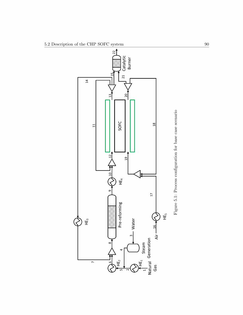
5.2 Description of the CHP SOFC system 90
Fig
ure
5.1:
Pro
cess
con
figu
rati
onfo
rb
ase
case
scen
ario

5.3 Mathematical Problem Formulation 91
respectively. In addition, typical high air ratios, used for cooling of the fuel cell, allow
for cathode recycling. Hence, the option of stream recycling increases the degrees of
freedom for process design and hence the design flexibility.
5.3 Mathematical Problem Formulation
5.3.1 Mathematical models
The mathematical model consists of a set of differential–algebraic equations (DAEs),
developed based on first principles (e.g. mass and energy balances) at steady–state.
Natural gas is assumed to be 100% methane and the operating pressure for the entire
CHP plant is fixed to atmospheric pressure. Given the low operating pressure, the use
of fluid transferring process units (e.g. fans, pumps) has been omitted in this analysis.
Other assumptions considered during the modeling of the CHP plant include: ideal gas
behavior, plug flow condition and complete conversion of unreacted fuels in the cat-
alytic burner. In addition, the SOFC stack consists of a number of single cells with a
uniform voltage distribution. A uniform temperature distribution has been assumed in
the pre–reforming unit imposed through distributed heating elements.
Pre–reformer:
The mass balances in the pre–reforming unit are:
∂Fi∂z
=∑j
νi,j Rj (5.1)
where i = (CH4, H2O, CO, CO2, H2), j = {smr,wgs}, νi,j is the stoichiometric
coefficient matrix and Rj refers to the reaction rates for the steam methane reforming
and water gas shift reactions [108]. Furthermore, F is the molar flowrate (mol/s) and

5.3 Mathematical Problem Formulation 92
z is the dimensionless length (z = z/LR) where LR corresponds to the length of the
pre–reforming unit. The methane conversion is determined using the following equation:
xCH4 = 1− FCH4(1)
FCH4(0)(5.2)
Solid Oxide Fuel Cell:
The mathematical model for an anode–supported intermediate temperature SOFC with
direct internal reforming has been adopted from [168]. In their work [168], the authors
developed a distributed mathematical model including mass balances in anode and
cathode channel and energy balances in each compartment of the SOFC (e.g. fuel/air
channels, electrodes/electrolyte, interconnect). For simplicity in this analysis, we as-
sume a uniform temperature across all compartments of the SOFC, therefore a single
energy balance is used for the entire SOFC. The mass and energy balances used in this
analysis are:
∂Fi∂z
=∑k
νi,k Rk (5.3)
∂
∂z
(∑i
FiMwiHi
)+ AelecVsofcJ = 0 (5.4)
where k = (elec, smr, wgs), Aelec denotes the electrochemically active area of the
fuel cell (m2), Vsofc is the voltage of the SOFC (V) and J refers to the current density
(A/m2). Hi represents the mass specific enthalpy (J/kg) of each component calculated
from the following equation:
Hi = ∆H◦f,i +
∫ T
Tref
Cpi(T )dT
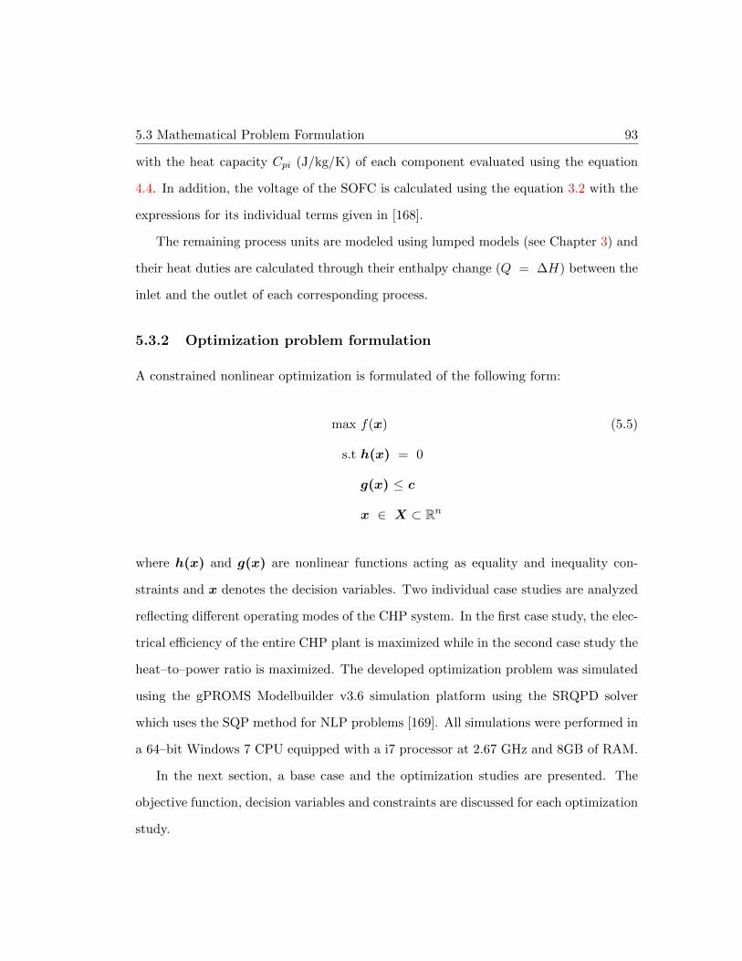
5.3 Mathematical Problem Formulation 93
with the heat capacity Cpi (J/kg/K) of each component evaluated using the equation
4.4. In addition, the voltage of the SOFC is calculated using the equation 3.2 with the
expressions for its individual terms given in [168].
The remaining process units are modeled using lumped models (see Chapter 3) and
their heat duties are calculated through their enthalpy change (Q = ∆H) between the
inlet and the outlet of each corresponding process.
5.3.2 Optimization problem formulation
A constrained nonlinear optimization is formulated of the following form:
max f(x) (5.5)
s.t h(x) = 0
g(x) ≤ c
x ∈ X ⊂ Rn
where h(x) and g(x) are nonlinear functions acting as equality and inequality con-
straints and x denotes the decision variables. Two individual case studies are analyzed
reflecting different operating modes of the CHP system. In the first case study, the elec-
trical efficiency of the entire CHP plant is maximized while in the second case study the
heat–to–power ratio is maximized. The developed optimization problem was simulated
using the gPROMS Modelbuilder v3.6 simulation platform using the SRQPD solver
which uses the SQP method for NLP problems [169]. All simulations were performed in
a 64–bit Windows 7 CPU equipped with a i7 processor at 2.67 GHz and 8GB of RAM.
In the next section, a base case and the optimization studies are presented. The
objective function, decision variables and constraints are discussed for each optimization
study.

5.4 Simulations 94
5.4 Simulations
5.4.1 Base case study
A base case study simulation (see Figure 5.1) is performed where no stream recycling is
considered. The operating conditions used in this simulation are shown in the following
table, where λair is the air ratio defined in [168], S/C is the steam–to–carbon ratio at
Table 5.1: Operating conditions for base case scenarioVariable Value Variable Value
UF (%) 85 Tca,in (K) 1023
Vsofc (V) 0.67 Tan,in (K) 1023
P (W/cm2) 0.4 mCHin4
(kg/h) 42.2
xCH4 (%) 10 λair 8.5
TR (K) 615 S/C 2
TCB (K) 1176 Ncell 104
the inlet of the pre–reformer and Ncell denotes the number of cells in the SOFC stack.
Figures 5.2 and 5.3 depict the species mole fractions and the temperature distribution
across the SOFC axial dimension. According to Figures 5.2 and 5.3, the high reaction
rates of the internal reforming reactions at the inlet of the anode lead to an increased
hydrogen concentration and a decreased temperature. However, there is a point (∼0.24)
where the internal reforming rate becomes equal to the hydrogen electrochemical reac-
tion rate. After that point, the hydrogen electrochemical reaction dominates consuming
hydrogen and releasing heat. This behavior results in an uneven temperature profile as
shown in the Figure 5.3.
5.4.2 Case study 1: Optimal design for maximized electrical efficiency
The electrical efficiency for the entire CHP plant is defined as ratio of the generated
power to the total chemical energy entering the plant calculated using the Lower Heating

5.4 Simulations 95
0 0.2 0.4 0.6 0.8 10
0.1
0.2
0.3
0.4
0.5
0.6
0.7
0.8
axial
mol
e fr
actio
n
:CH
4
:H2O
:CO:CO
2
:H2
:O2
Figure 5.2: Species mole fraction distribution in anode and cathode of the SOFC
Value (LHV) of the fuel (e.g. methane):
f(x) =AelecVstackJ
F inCH4LHVCH4
(5.6)
Typically, AC power is used in the system’s electrical efficiency calculation [170], however
this study does not consider any integration of power electronics (e.g. DC/AC converter)
downstream to the SOFC hence the DC power generated from the SOFC is used. The
following recycle ratios are defined:
anode: ASR =mi
m13where: i = 11, 14, 15 (5.7)
cathode: CSR =mj
m20where: j = 18, 21 (5.8)

5.4 Simulations 96
0 0.2 0.4 0.6 0.8 1
1000
1020
1040
1060
1080
1100
1120
axial
Tem
pera
ture
(K
)
Figure 5.3: SOFC temperature distribution
where ASR and CSR refer to anode and cathode stream ratio respectively, m denotes
the mass flowrate (kg/s) and the subscripts refer to the streams in Figure 5.1.
The decision variables used in this simulation are the following:
x =
[ASR1 ASR2 ASR3 CSR1 CSR2 T6 T7 xCH4 UF Vsofc T12 T19
]T(5.9)
where ASR3 ∈[0.05,1] to ensure a minimum feed of unreacted fuel to the catalytic
burner and the remaining recycle ratios ∈[0,1]. xCH4 ∈[0.05,1] in order to prevent any
feed of pure methane to the SOFC anode. UF ∈[75,85] in order to maintain a sufficient
level of fuel utilization and avoid fuel starvation conditions. Vsofc ∈[0.6,0.7] since we
would like to operate the SOFC in a common voltage range for direct internal reforming
SOFC. T12 ∈[973,1073] and T19 ∈[973,1073] to ensure an appropriate SOFC operating
temperature. T7 is lower bounded by 298 K to avoid excessive cooling while T6 is lower

5.4 Simulations 97
bounded by 373 K in order to prevent any cooling below the water bubble point.
In addition to the mathematical model of the CHP plant, which acts as equality
constraint in the optimization problem, the following equality and inequality constraints
are included:
•3∑i=1
ASRi = 1: The sum of all recycle ratios at the anode should always be equal
to unity
•2∑j=1
CSRj = 1: The sum of all recycle ratios at the cathode should always be equal
to unity
• F inO2,cb> 0 mol/s: Maintain oxygen supply to the catalytic burner
• F inH2O,feed≥0 mol/s: Prevent negative inlet water flowrates
• Tsofc(1)≤1173 K: Limit the SOFC outlet temperature to 1173 K
• T17≥298 K: Prevent any cooling of air below ambient conditions
• 0.35 W/cm2≤Psofc≤1 W/cm2: Ensure an operation under reasonable power den-
sities
• 0 K≤∆TR,max≤50 K: Maintain a small temperature difference in pre–reforming
unit
• 0 K≤∆Tsofc,max≤150 K: Prevent large temperature gradients across the SOFC
The optimal solution corresponds to a system electrical efficiency of 64.5%. The op-
timal values for the decision variables are shown in Table 5.2 and the optimal design is
depicted in Figure 5.4. The main findings of this simulation include the large contribu-
tion of the anode recycles and the elimination of the steam generation unit. More than
half of the stream leaving the anode is recycled back to the pre–reforming unit where a

5.4 Simulations 98
Table 5.2: Case study 1: optimal values for the decision variablesVariable Value Variable Value
ASR1 0.23 T7 (K) 956.72
ASR2 0.53 xCH4 (%) 37.7
ASR3 0.24 UF (%) 85
CSR1 1 Vsofc (V) 0.7
CSR2 0 T12 (K) 1073
T6 (K) 376.15 T19 (K) 1073
methane conversion of 37.7% is achieved. This recycle satisfies the required S/C ratio
at the inlet of the pre–reforming unit allowing for a sustainable operation in terms of
steam generation. In addition, 24% of the anode outlet stream is recycled back to the
anode in order to improve the system electrical efficiency. The optimal operating condi-
tions of the SOFC show the attempt of the system to maximize the electrical efficiency
since the SOFC operates at the upper bounds of the fuel utilization and the operating
voltage which potentially leads to a higher power density. In addition to this, both
the anode and cathode inlet temperatures reach their upper bounds trying to increase
the SOFC operating temperature in order to increase the electronic conductivity of the
electrolyte and hence the SOFC performance. However, it should be mentioned that
this increase of the cathode temperature compared to the base case, results in a higher
air pre–heating duty which dominates the energy demand for pre–heating. Considering
also its high temperature, energy integration could be challenging.
5.4.3 Case study 2: Maximizing the heat–to–power ratio
The heat–to–power ratio is defined as the net heat to the generated power. The net heat
of the CHP plant is calculated as the difference of the total available heat generated and

5.4 Simulations 99
Fig
ure
5.4:
Op
tim
ald
esig
nfo
rm
axim
ized
elec
tric
aleffi
cien
cy

5.4 Simulations 100
the heating loads for the streams pre–heating and the pre–reformer heating requirement:
f(x) =Qtotal − QheatingAelecVstackJ
(5.10)
The decision variables used in this simulation are shown below in vector form:
x =
[ASR1 ASR2 ASR3 CSR1 CSR2 T7 xCH4 UF Vsofc T12 T19
]T(5.11)
The same bounds as in the previous case study are considered. In terms of constraints,
most of the previous constraints hold while a constraint considered above is changed.
In addition to this, two new constraints are imposed. The additional constraints are:
• F inH2O,feed=0 mol/s: Maintain a self–sustained operation in terms of steam gener-
ation
• 0 kW≤Pstack≤300 kW: Ensure a comparable output power with the previous case
studies
• 50 %≤ηelectrical≤100 %: Retain a highly efficient operation
The optimal solution is attained for a heat–to–power ratio equal to 0.92. The values
of the decision variables at the optimal solution are presented in Table 5.3 and the
optimal design is shown in Figure 5.5. According to the results, the main features of
Table 5.3: Case study 2: optimal values for the decision variablesVariable Value Variable Value
ASR1 0.43 T7 (K) 947
ASR2 0.53 xCH4 (%) 35.9
ASR3 0.04 UF (%) 75
CSR1 0.07 Vsofc (V) 0.6
CSR2 0.93 T12 (K) 973
T19 (K) 999

5.4 Simulations 101
the CHP plant include its attempt to reduce the heating loads and maintain a large
supply of unreacted fuels to the catalytic burner for increased heat generation. In
order to ensure a sustainable operation in terms of steam generation, 53% of the anode
outlet stream is recycled back to the pre–reforming unit. In addition, the anode recycle
ratio has been decreased from 24% in the previous study to 4% in order to satisfy the
constraint on the system’s electrical efficiency. On the other hand, the cathode recycle
ratio has increased from 0% to 97% eliminating the need for air pre–heating since the
required cathode inlet temperature is achieved by mixing the recycling stream with
fresh air. The SOFC operates at a lower fuel utilization in order to allow for more
heat generation in the catalytic burner. Furthermore, the anode and cathode inlet
temperatures have been decreased leading to lower heating loads while satisfying the
SOFC operating constraints.
5.4.4 Comparison of SOFC temperature distribution
Figure 5.6 depicts the normalized SOFC temperature distributions for each case study.
Since both optimal designs are obtained with a pre–reforming conversion higher than
the base case scenario (37.7% and 35.9% to 10%), it is expected that they exhibit a
smoother temperature profile than the base case scenario as shown in Figure 5.6. Apart
from the effect of the higher pre–reforming conversion, the anode recycle influences the
shape of the temperature distributions leading to lower temperature gradients across
the SOFC. Higher concentrations of hydrogen at the inlet of the anode channel result in
more energy released due to the electrochemical reactions. Considering also the reduced
concentration of methane at the inlet of the anode channel the temperature gradient is
decreased.
According to Figure 5.6, the temperature distribution associated with the optimal
design of the second case study shows a smoother temperature distribution compared to

5.4 Simulations 102
Fig
ure
5.5:
Op
tim
ald
esig
nfo
rm
axim
ized
hea
t–to
–pow
erra
tio

5.4 Simulations 103
0 0.2 0.4 0.6 0.8 10.88
0.9
0.92
0.94
0.96
0.98
1
axial
Nor
mal
ized
Tem
pera
ture
:Base case:max(Heat/Power):max(η
electrical)
Figure 5.6: Comparison of SOFC temperature distribution for each case study
the other cases. Although a lower pre–reforming conversion is achieved compared to the
first case study, the lower SOFC inlet temperatures lead to slower internal reforming
reaction kinetics. In addition to this, the lower fuel utilization prevents any sharp
increase in the temperature compared to the other two cases.

CHAPTER 6
Summary and Future Directions
Motivated by the need for highly efficient and environmentally friendly power genera-
tion, this dissertation focuses on the design and control of integrated systems for hydro-
gen production and power generation. Two integration strategies, energy integration
and process intensification, were considered since they have shown a great potential for
increased energy efficiency. In addition, SOFC systems were designed employing the
above integration strategies and challenges in terms of design, operation and control
were identified and solutions were proposed.
In the first part of the thesis, two energy integrated configurations were analyzed
comprising a SOFC, a methane steam reformer and energy transfer units. In the first
configuration, the SOFC outlet streams were used directly for energy integration, while
in the second, these streams were fed to a catalytic burner for more energy recovery
and recycle. The first configuration was shown to become unstable for large changes in
104

6 Summary and Future Directions 105
current. This was attributed to a positive energy feedback loop which results in high
temperatures and fuel starvation. A linear multi-loop control strategy was developed for
the entire integrated system. The proposed control strategy was shown to be successful
in suppressing the instability in the first configuration and to provide satisfactory closed-
loop responses for a broad range of positive and negative changes in the current.
The use of process intensification for simultaneous hydrogen generation and carbon
capture has brought water gas shift (WGS) membrane reactors to the forefront as an
emerging technology. Thermal management in these type of reactors is essential for
maintaining the reactor’s performance at desired conditions. In the second part of
the thesis, a dynamic model for a hydrogen–selective WGS membrane reactor for the
production of high-purity hydrogen was developed and a distributed control strategy
was proposed for regulating the temperature along the reactor. The strategy involved
distributed actuation with cooling zones placed judiciously along the reactor and a
model-based output feedback controller derived on the basis of the distributed process
model. The controller was shown to be successful in suppressing hot spots that can be
detrimental to the reactor performance, in the presence of disturbances and set point
changes. A comparison with classical PI controllers demonstrated the benefit of using
model-based control even in the presence of modeling errors.
The ability of SOFCs for combined heat and power (CHP) generation has attracted
a lot of attention as a promising option for distributed generation. Design flexibility
of CHP SOFC systems is essential in order to ensure a continuous and reliable source
of energy under a volatile energy market. The CHP SOFC system considered in the
thesis includes a direct internal reforming SOFC along with a pre–reforming unit before
the SOFC. The option for multiple recycle loops in the CHP configuration has been a
key factor in design flexibility. A nonlinear optimization problem was formulated and
optimal designs were obtained for different operating modes. The preliminary results

6 Summary and Future Directions 106
showed that a systems level optimization formulation including recycle ratios as decision
variables can successfully evaluate optimal operating conditions for different operational
objectives.
In addition to the previous study in CHP SOFC, further design objectives should
be considered in order to allow for broader insights. Therefore, the previous design
analysis should include energy integration by reformulating the optimization problem.
It is expected that this reformulation would transform the previously developed nonlin-
ear program (NLP) to a mixed–integer nonlinear program (MINLP). Optimal bypass
placement in the new attained energy integrated configuration would allow for control
studies. Developing a real time optimizer (RTO) as a supervisory controller would al-
low for an optimal operation based on either economical or environmental objectives.
Optional integration of the CHP SOFC system with renewable energy resources would
allow for a lower environmental impact. Additional integration with power and thermal
storage units would further increase the flexibility of the CHP SOFC system.
In terms of large–scale power plants, system’s level analysis for integration of SOFCs
with conventional power plants (e.g IGCC, NGCC) and options for additional integra-
tion with biomass are expected to attract a lot of attention. Improving operability and
ensuring a robust system’s response under various disturbances would lead to attractive
solutions for future power generation systems.

Bibliography
[1] NETL. Fuel Cell Handbook 7th Edition. U.S. Department of Energy, 2004.
[2] Comparison of Fuel Cell Technologies. http://www1.eere.energy.gov/
hydrogenandfuelcells/fuelcells/pdfs/fc_comparison_chart.pdf. Ac-cessed: 10-21-2013.
[3] National Energy Technology Laboratory. Cost and performance baseline for fossilenergy plants volume 1: Bituminous coal and natural gas to electricity. TechnicalReport 2010/1397, DOE NETL, USA, November 2010.
[4] SECA A Primer on SOFC Technology. http://www.netl.doe.gov/
technologies/coalpower/fuelcells/seca/primer/cell.html. Accessed: 11-11-2013.
[5] http://mech-server.mech.kyoto-u.ac.jp/lab/yoshida/b4intro/nishino/
tubularE4.jpg. Accessed: 11-11-2013.
[6] Dimitrios Georgis, Fernando V Lima, Ali Almansoori, and Prodromos Daoutidis.Modeling and control of a water gas shift membrane reactor for hydrogen pro-duction. In American Control Conference (ACC), 2012, pages 4287–4292. IEEE,2012.
[7] Core Writing Team, Pachauri, R.K. and Reisinger, A. (Eds.). Climate change2007: Synthesis report. Technical report, IPCC, Geneva, Switzerland, November2007.
[8] U.S Environmental Protecting Agency. Inventory of u.s greenhouse gas emissionsand sinks: 1990–2010. Technical Report 430–R–12–001, EPA, Washington, DC,April 2012.
107

BIBLIOGRAPHY 108
[9] OECD Stat. Exacts. http://stats.oecd.org/Index.aspx?DataSetCode=AIR_
GHG. Accessed: 10-17-2013.
[10] OECD. Environmental outlook to 2030. Technical report, OECD, Paris, France,2008.
[11] WEC. World energy insight 2012. Technical report, WEC, London, UK, 2012.
[12] BP. Energy outlook 2030. Technical report, BP, London, UK, 2013.
[13] International Energy Agency. Key world energy statistics. Technical report,OECD/IEA, Paris, 2013.
[14] U.S Energy Information Administration. http://www.eia.gov/tools/faqs/
faq.cfm?id=105&t=3. Accessed: 10-03-2013.
[15] Coal Industry Advisory Board. Power generation from coal: Measuring and re-porting efficiency performance and co2 emissions. Technical report, OECD IEA,France, 2010.
[16] U.S Fuel Economy Information. http://www.fueleconomy.gov/feg/atv.shtml.Accessed: 10-03-2013.
[17] Ram Ramachandran and Raghu K. Menon. An overview of industrial uses ofhydrogen. International Journal of Hydrogen Energy, 23(7):593–598, 1998.
[18] John A. Turner. Sustainable hydrogen production. Science, 305(5686):972–974,2004.
[19] Committee on Alternatives, Strategies for Future Hydrogen Production, and Na-tional Academy of Engineering Use, National Research Council. The Hydro-gen Economy: Opportunities, Costs, Barriers, and R&D Needs. The NationalAcademies Press, 2004.
[20] Magdalena Momirlan and T. Nejat Veziroglu. The properties of hydrogen as fueltomorrow in sustainable energy system for a cleaner planet. International Journalof Hydrogen Energy, 30(7):795–802, 2005.
[21] Fuel Cell Vehicles. http://www.fuelcells.org/uploads/carchart.pdf. Ac-cessed: 10-12-2013.
[22] Steven G. Chalk, James F. Miller, and Fred W. Wagner. Challenges for fuel cellsin transport applications. Journal of Power Sources, 86(1):40–51, 2000.
[23] Panini Krishna Kolavennu. Analysis and control of an in situ hydrogen generationand fuel cell power system for automotive applications. PhD thesis, Florida StateUniversity, December 2005.

BIBLIOGRAPHY 109
[24] Dimitrios Georgis, Sujit S Jogwar, Ali Almansoori, and Prodromos Daoutidis. De-sign and control of energy integrated SOFC systems for in–situ hydrogen produc-tion and power generation. Computers & Chemical Engineering, 35(9):1691–1704,2011.
[25] Peter P. Edwards, Vladimir L. Kuznetsov, William I.F. David, and Nigel P. Bran-don. Hydrogen and fuel cells: towards a sustainable energy future. Energy Policy,36(12):4356–4362, 2008.
[26] S. Litster and G. McLean. PEM fuel cell electrodes. Journal of Power Sources,130(1):61–76, 2004.
[27] Chunshan Song. Fuel processing for low–temperature and high-temperature fuelcells: Challenges, and opportunities for sustainable development in the 21st cen-tury. Catalysis Today, 77(1):17–49, 2002.
[28] Yuyan Shao, Geping Yin, Zhenbo Wang, and Yunzhi Gao. Proton exchange mem-brane fuel cell from low temperature to high temperature: material challenges.Journal of Power Sources, 167(2):235–242, 2007.
[29] Jianlu Zhang, Zhong Xie, Jiujun Zhang, Yanghua Tang, Chaojie Song, TitichaiNavessin, Zhiqing Shi, Datong Song, Haijiang Wang, David P Wilkinson, Zhong-Sheng Liu, and Steven Holdcroft. High temperature PEM fuel cells. Journal ofPower Sources, 160(2):872–891, 2006.
[30] Brian C.H. Steele and Angelika Heinzel. Materials for fuel-cell technologies. Na-ture, 414(6861):345–352, 2001.
[31] K.D. Kreuer. On the development of proton conducting polymer membranes forhydrogen and methanol fuel cells. Journal of Membrane Science, 185(1):29–39,2001.
[32] Subhash Singhal and Kevin Kendall. High–temperature Solid Oxide Fuel Cells:Fundamentals, Design and Applications: Fundamentals, Design and Applications.Elsevier, 2003.
[33] X. Li. Principles of Fuel Cells. Taylor & Francis Group, 2006.
[34] Nurettin Demirdoven and John Deutch. Hybrid cars now, fuel cell cars later.Science, 305(5686):974–976, 2004.
[35] Patrick Linke, Antonis Kokossis, and Alberto Alva-Argaez. Process intensification.Computer Aided Process and Product Engineering (CAPE), 1, 2007.
[36] Andrzej Stankiewicz and Jacob A. Moulijn. Process intensification: transformingchemical engineering. Chemical Engineering Progress, pages 22–34, 2000.

BIBLIOGRAPHY 110
[37] Andrzej Stankiewicz and Jacob A. Moulijn. Process intensification. Industrial &Engineering Chemistry Research, 41(8):1920–1924, 2002.
[38] David Reay, Colin Ramshaw, and Adam Harvey. Process Intensification: En-gineering for efficiency, sustainability and flexibility. Butterworth-Heinemann,2013.
[39] Nikola M. Nikacevic, Adrie E.M. Huesman, Paul M.J. Van den Hof, and Andrzej I.Stankiewicz. Opportunities and challenges for process control in process intensi-fication. Chemical Engineering and Processing: Process Intensification, 52:1–15,2012.
[40] Jacob A Moulijn, Andrzej Stankiewicz, Johan Grievink, and Andrzej Gorak. Pro-cess intensification and process systems engineering: a friendly symbiosis. Com-puters & Chemical Engineering, 32(1):3–11, 2008.
[41] Kari Alanne and Arto Saari. Sustainable small-scale CHP technologies for build-ings: the basis for multi-perspective decision-making. Renewable and SustainableEnergy Reviews, 8(5):401–431, 2004.
[42] H.I. Onovwiona and V.I. Ugursal. Residential cogeneration systems: review ofthe current technology. Renewable and Sustainable Energy Reviews, 10(5):389–431, 2006.
[43] Reinhard Madlener and Christiane Schmid. Combined heat and power generationin liberalised markets and a carbon-constrained world. GAIA-Ecological Perspec-tives for Science and Society, 12(2):114–120, 2003.
[44] Pilar Lisbona, Alessandro Corradetti, Roberto Bove, and Piero Lunghi. Analysisof a solid oxide fuel cell system for combined heat and power applications undernon-nominal conditions. Electrochimica Acta, 53(4):1920–1930, 2007.
[45] D.W. Wu and R.Z. Wang. Combined cooling, heating and power: A review.Progress in Energy and Combustion Science, 32(5):459–495, 2006.
[46] Guido Pepermans, Johan Driesen, Dries Haeseldonckx, Ronnie Belmans, andWilliam Dhaeseleer. Distributed generation: definition, benefits and issues. En-ergy Policy, 33(6):787–798, 2005.
[47] Anne Hampson. Combined heat and power: Enabling resilient energy infrastruc-ture for critical facilities. Technical Report ORNL/TM–2013/100, Oak RidgeNational Laboratory (ORNL), March 2013.
[48] A.D. Hawkes, P. Aguiar, B. Croxford, M.A. Leach, C.S. Adjiman, and N.P. Bran-don. Solid oxide fuel cell micro combined heat and power system operating strat-egy: Options for provision of residential space and water heating. Journal ofPower Sources, 164(1):260–271, 2007.
BIBLIOGRAPHY 111
[49] Erkko Fontell, Timo Kivisaari, N. Christiansen, J-B Hansen, and J. Palsson. Con-ceptual study of a 250kW planar SOFC system for CHP application. Journal ofPower Sources, 131(1):49–56, 2004.
[50] Gianfranco Chicco and Pierluigi Mancarella. Distributed multi-generation: a com-prehensive view. Renewable and Sustainable Energy Reviews, 13(3):535–551, 2009.
[51] Residential Energy Consumption Survey U.S. Energy Information Adminis-tration. Heating and cooling no longer majority of U.S home energy use.http://www.eia.gov/todayinenergy/detail.cfm?id=10271&src=%E2%80%B9%
20Consumption%20%20%20%20%20%20Residential%20Energy%20Consumption%
20Survey%20(RECS)-b1. Accessed: 10-26-2013.
[52] Whitney Colella. Implications of electricity liberalization for combined heat andpower (CHP) fuel cell systems (FCS): a case study of the United Kingdom. Journalof Power Sources, 106(1):397–404, 2002.
[53] Whitney Colella. Design options for achieving a rapidly variable heat-to-powerratio in a combined heat and power (CHP) fuel cell system (FCS). Journal ofPower Sources, 106(1):388–396, 2002.
[54] Ernst Riensche, Josefin Meusinger, Ulrich Stimming, and Guido Unverzagt. Op-timization of a 200 kW SOFC cogeneration power plant. part II: variation of theflowsheet. Journal of Power Sources, 71(1):306–314, 1998.
[55] R.J. Braun, S.A. Klein, and D.T. Reindl. Evaluation of system configurations forsolid oxide fuel cell-based micro-combined heat and power generators in residentialapplications. Journal of Power Sources, 158(2):1290–1305, 2006.
[56] Tae Seok Lee, J.N. Chung, and Yen-Cho Chen. Design and optimization of a com-bined fuel reforming and solid oxide fuel cell system with anode off-gas recycling.Energy Conversion and Management, 52(10):3214–3226, 2011.
[57] Shiying Lin, Michiaki Harada, Yoshizo Suzuki, and Hiroyuki Hatano. Hydro-gen production from coal by separating carbon dioxide during gasification. Fuel,81(16):2079–2085, 2002.
[58] Jens R Rostrup-Nielsen. Production of synthesis gas. Catalysis today, 18(4):305–324, 1993.
[59] A. Boudghene Stambouli and E. Traversa. Solid oxide fuel cells (SOFCs): areview of an environmentally clean and efficient source of energy. Renewable andSustainable Energy Reviews, 6(5):433–455, 2002.
[60] Andrew L. Dicks. Hydrogen generation from natural gas for the fuel cell systemsof tomorrow. Journal of Power Sources, 61(1):113–124, 1996.
BIBLIOGRAPHY 112
[61] P. Aguiar, D. Chadwick, and L. Kershenbaum. Modelling of an indirect internalreforming solid oxide fuel cell. Chemical Engineering Science, 57(10):1665–1677,2002.
[62] Khaliq Ahmed and Karl Foger. Kinetics of internal steam reforming of methaneon ni/ysz-based anodes for solid oxide fuel cells. Catalysis Today, 63(2):479–487,2000.
[63] Caine M. Finnerty, Neil J. Coe, Robert H. Cunningham, and R. Mark Ormerod.Carbon formation on and deactivation of nickel-based/zirconia anodes in solidoxide fuel cells running on methane. Catalysis Today, 46(2):137–145, 1998.
[64] Vinod M. Janardhanan and Olaf Deutschmann. CFD analysis of a solid oxidefuel cell with internal reforming: Coupled interactions of transport, heterogeneouscatalysis and electrochemical processes. Journal of Power Sources, 162(2):1192–1202, 2006.
[65] S. Campanari and P. Iora. Definition and sensitivity analysis of a finite volumeSOFC model for a tubular cell geometry. Journal of Power Sources, 132(1):113–126, 2004.
[66] Mona Bavarian and Masoud Soroush. Steady–state multiplicity in a solid oxidefuel cell: Practical considerations. Chemical Engineering Science, 67(1):2–14,2012.
[67] W. Lehnert, J. Meusinger, and F. Thom. Modelling of gas transport phenomenain SOFC anodes. Journal of Power Sources, 87(1):57–63, 2000.
[68] Thinh X. Ho, Pawel Kosinski, Alex C. Hoffmann, and Arild Vik. Numerical anal-ysis of a planar anode-supported SOFC with composite electrodes. InternationalJournal of Hydrogen Energy, 34(8):3488–3499, 2009.
[69] Ryan P O’Hayre, Suk-Won Cha, Whitney Colella, and Fritz B Prinz. Fuel cellfundamentals. John Wiley & Sons New York, 2006.
[70] Zuo Chendong, Liu Mingfei, and Liu Meilin. Chapter 2: Solid oxide fuel cells. InMario Aparicio, Andrei Jitianu, and Lisa C Klein, editors, Sol-Gel processing forconventional and alternative energy, Advances in Sol-Gel Derived Materials andTechnologies, pages 7–35. Springer, 2012.
[71] JPP Huijsmans, FPF Van Berkel, and GM Christie. Intermediate temperatureSOFC–a promise for the 21st century. Journal of Power Sources, 71(1):107–110,1998.
[72] R Mark Ormerod. Solid oxide fuel cells. Chemical Society Reviews, 32(1):17–28,2003.

BIBLIOGRAPHY 113
[73] Vincenzo Liso, Anders Christian Olesen, Mads Pagh Nielsen, and Søren KnudsenKær. Performance comparison between partial oxidation and methane steamreforming processes for solid oxide fuel cell (SOFC) micro combined heat andpower (CHP) system. Energy, 36(7):4216–4226, 2011.
[74] Michael Baldea and Prodromos Daoutidis. Dynamics and control of autother-mal reactors for the production of hydrogen. Chemical Engineering Science,62(12):3218–3230, 2007.
[75] Seungdoo Park, John M Vohs, and Raymond J Gorte. Direct oxidation of hydro-carbons in a solid-oxide fuel cell. Nature, 404(6775):265–267, 2000.
[76] S McIntosh, JM Vohs, and RJ Gorte. Role of hydrocarbon deposits in the en-hanced performance of direct-oxidation SOFCs. Journal of The ElectrochemicalSociety, 150(4):470–476, 2003.
[77] E Perry Murray, T Tsai, and SA Barnett. A direct-methane fuel cell with aceria-based anode. Nature, 400(6745):649–651, 1999.
[78] Steven McIntosh and Raymond J Gorte. Direct hydrocarbon solid oxide fuel cells.Chemical Reviews, 104(10):4845–4866, 2004.
[79] Alan Atkinson, S Barnett, Raymond J Gorte, JTS Irvine, Augustin J McEvoy,Mogens Mogensen, Subhash C Singhal, and J Vohs. Advanced anodes for high-temperature fuel cells. Nature materials, 3(1):17–27, 2004.
[80] Dimitrios Georgis, Sujit S Jogwar, Ali S Almansoori, and Prodromos Daoutidis.Impact of steam reformer on the design and control of an energy integrated solidoxide fuel cell system. In 19th Mediterranean Conference on Control & Automation(MED), pages 576–581. IEEE, 2011.
[81] Subbarao Varigonda and Mithun Kamat. Control of stationary and transportationfuel cell systems: Progress and opportunities. Computers & Chemical Engineering,30(10-12):1735–1748, 2006.
[82] Jay T. Pukrushpan, Anna G. Stefanopoulou, and Huei Peng. Control of fuelcell power systems: principles, modeling, analysis, and feedback design. SpringerVerlag, 2004.
[83] D.L. Cresswell and I.S. Metcalfe. Energy integration strategies for solid oxide fuelcell systems. Solid State Ionics, 177(19-25):1905–1910, 2006.
[84] R.J. Kee, H. Zhu, A.M. Sukeshini, and G.S. Jackson. Solid oxide fuel cells: Op-erating principles, current challenges, and the role of syngas. Combustion Scienceand Technology, 180(6):1207–1244, 2008.

BIBLIOGRAPHY 114
[85] Debangsu Bhattacharyya and Raghunathan Rengaswamy. A review of solid oxidefuel cell (SOFC) dynamic models. Industrial & Engineering Chemistry Research,48(13):6068–6086, 2009.
[86] Mona Bavarian, Masoud Soroush, Ioannis G. Kevrekidis, and Jay B. Benziger.Mathematical Modeling, Steady-State and Dynamic Behavior, and Control of FuelCells: A Review. Industrial & Engineering Chemistry Research, 49(17):7922–7950,2010.
[87] A. Chaisantikulwat, C. Diaz-Goano, and E.S. Meadows. Dynamic modelling andcontrol of planar anode-supported solid oxide fuel cell. Computers & ChemicalEngineering, 32(10):2365–2381, 2008.
[88] A.K.M. Murshed, Biao Huang, and Kumar Nandakumar. Control relevant mod-eling of planer solid oxide fuel cell system. Journal of Power Sources, 163(2):830–845, 2007.
[89] Thomas A. Adams II and Paul I. Barton. High-efficiency power production fromnatural gas with carbon capture. Journal of Power Sources, 195(7):1971–1983,2010.
[90] Fabian Mueller, Faryar Jabbari, Robert Gaynor, and Jacob Brouwer. Novel solidoxide fuel cell system controller for rapid load following. Journal of Power Sources,172(1):308–323, 2007.
[91] Ayman M. Al-Qattan and Donald J. Chmielewski. Distributed feed design forSOFCs with internal reforming. Journal of the Electrochemical Society, 151:A1891,2004.
[92] Xiongwen Zhang, S.H. Chan, Guojun Li, H.K. Ho, Jun Li, and Zhenping Feng. Areview of integration strategies for solid oxide fuel cells. Journal of Power Sources,195(3):685–702, 2010.
[93] S.H. Chan, H.K. Ho, and Y. Tian. Modelling of simple hybrid solid oxide fuel celland gas turbine power plant. Journal of Power Sources, 109(1):111–120, 2002.
[94] Xiongwen Zhang, Jun Li, Guojun Li, and Zhenping Feng. Dynamic modeling ofa hybrid system of the solid oxide fuel cell and recuperative gas turbine. Journalof Power Sources, 163(1):523–531, 2006.
[95] M. Cali, M.G.L. Santarelli, and P. Leone. Computer experimental analysis of theCHP performance of a 100 kWe SOFC Field Unit by a factorial design. Journalof Power Sources, 156(2):400–413, 2006.

BIBLIOGRAPHY 115
[96] Yaofan Yi, Ashok D. Rao, Jacob Brouwer, and G. Scott Samuelsen. Fuel flexibilitystudy of an integrated 25kW SOFC reformer system. Journal of power sources,144(1):67–76, 2005.
[97] R. Kandepu, L. Imsland, B.A. Foss, C. Stiller, B. Thorud, and O. Bolland.Modeling and control of a SOFC-GT-based autonomous power system. Energy,32(4):406–417, 2007.
[98] Fabian Mueller, Robert Gaynor, Allie E. Auld, Jacob Brouwer, Faryar Jabbari,and G. Scott Samuelsen. Synergistic integration of a gas turbine and solid oxidefuel cell for improved transient capability. Journal of Power Sources, 176(1):229–239, 2008.
[99] S.R. Oh and J. Sun. Optimization and load-following characteristics of 5kw-classtubular solid oxide fuel cell/gas turbine hybrid systems. In American ControlConference (ACC), 2010, pages 417–422. IEEE, 2010.
[100] P. Varbanov and J. Klemes. Analysis and integration of fuel cell combined cyclesfor development of low-carbon energy technologies. Energy, 33(10):1508–1517,2008.
[101] Jhuma Sadhukhan, Yingru Zhao, Matthew Leach, Nigel P Brandon, and NilayShah. Energy integration and analysis of solid oxide fuel cell based microcombinedheat and power systems and other renewable systems using biomass waste derivedsyngas. Industrial & Engineering Chemistry Research, 49(22):11506–11516, 2010.
[102] D.J. Bents. High temperature solid oxide regenerative fuel cell for solar photo-voltaic energy storage. In Proceedings of the 22nd Intersociety Energy ConversionEngineering Conference, pages 808–817. AIAA, 1987.
[103] C.H. Hamann, A. Hamnett, and W. Vielstich. Electrochemistry. Weinheim: Wiley-VCH, 2007.
[104] C. Wang and M.H. Nehrir. A physically based dynamic model for solid oxide fuelcells. IEEE Transactions on Energy Conversion, 22(4):887–897, 2007.
[105] J.R. Ferguson, J.M. Fiard, and R. Herbin. Three-dimensional numerical simu-lation for various geometries of solid oxide fuel cells. Journal of Power Sources,58(2):109–122, 1996.
[106] Handa Xi, Subbarao Varigonda, and Buyun Jing. Dynamic modeling of a Solid Ox-ide Fuel Cell system for control design. In American Control Conference (ACC),2010, pages 423–428. IEEE, 2010.

BIBLIOGRAPHY 116
[107] M. Sorrentino, C. Pianese, and Y.G. Guezennec. A hierarchical modeling approachto the simulation and control of planar solid oxide fuel cells. Journal of PowerSources, 180(1):380–392, 2008.
[108] J. Xu and G.F. Froment. Methane steam reforming, methanation and water-gasshift: I. Intrinsic kinetics. AIChE Journal, 35(1):88–96, 1989.
[109] B. Linnhoff and E. Hindmarsh. The pinch design method for heat exchangernetworks. Chemical Engineering Science, 38(5):745–763, 1983.
[110] Ian C. Kemp. Pinch analysis and process integration: a user guide on processintegration for the efficient use of energy. Butterworth-Heinemann, 2007.
[111] William L. Luyben. Process modeling, simulation, and control for chemical engi-neers. McGraw-Hill New York, 1990.
[112] Reyyan Koc, Nikolaos K. Kazantzis, William J. Nuttall, and Yi Hua Ma. Eco-nomic assessment of inherently safe membrane reactor technology options inte-grated into IGCC power plants . Process Safety and Environmental Protection,90(5):436 – 450, 2012.
[113] C. Descamps, C. Bouallou, and M. Kanniche. Efficiency of an integrated gasi-fication combined cycle (IGCC) power plant including CO2 removal. Energy,33(6):874 – 881, 2008.
[114] Kendell R. Jillson, Vishnu Chapalamadugu, and B. Erik Ydstie. Inventory andflow control of the IGCC process with CO2 recycles. Journal of Process Control,19(9):1470 – 1485, 2009.
[115] F. Emun, M. Gadalla, T. Majozi, and D. Boer. Integrated gasification combinedcycle (IGCC) process simulation and optimization. Computers & Chemical Engi-neering, 34(3):331–338, 2010.
[116] Thomas A Adams II and Paul I Barton. High-efficiency power production fromnatural gas with carbon capture. Journal of Power Sources, 195(7):1971–1983,2010.
[117] Fabian Mueller, Faryar Jabbari, and Jacob Brouwer. On the intrinsic transient ca-pability and limitations of solid oxide fuel cell systems. Journal of Power Sources,187(2):452–460, 2009.
[118] W.L. Becker, R.J. Braun, M. Penev, and M. Melaina. Design and technoeconomicperformance analysis of a 1MW solid oxide fuel cell polygeneration system forcombined production of heat, hydrogen, and power. Journal of Power Sources,200(0):34 – 44, 2012.

BIBLIOGRAPHY 117
[119] Thomas A Adams II and Paul I Barton. Combining coal gasification, natural gasreforming, and solid oxide fuel cells for efficient polygeneration with CO2 captureand sequestration. Fuel Processing Technology, 92(10):2105 – 2115, 2011.
[120] Mu Li, Jacob Brouwer, Ashok D Rao, and G Scott Samuelsen. Application of adetailed dimensional solid oxide fuel cell model in integrated gasification fuel cellsystem design and analysis. Journal of Power Sources, 196(14):5903–5912, 2011.
[121] Thomas A Adams II and Paul I Barton. A dynamic two–dimensional hetero-geneous model for water gas shift reactors. International Journal of HydrogenEnergy, 34(21):8877–8891, 2009.
[122] Jose D. Figueroa, Timothy Fout, Sean Plasynski, Howard McIlvried, and Ramesh-war D. Srivastava. Advances in CO2 capture technology–the U.S. Department ofEnergy’s Carbon Sequestration Program. International Journal of GreenhouseGas Control, 2(1):9 – 20, 2008.
[123] TE Rufford, S Smart, GCY Watson, BF Graham, J Boxall, JC Diniz da Costa, andEF May. The removal of CO2 and N2 from natural gas: A review of conventionaland emerging process technologies. Journal of Petroleum Science and Engineering,94–95(0):123–154, 2012.
[124] M. De Falco, L. Di Paola, L. Marrelli, and P. Nardella. Simulation of large-scalemembrane reformers by a two-dimensional model. Chemical Engineering Journal,128(2):115–125, 2007.
[125] Rune Bredesen, Kristin Jordal, and Olav Bolland. High-temperature membranesin power generation with co2 capture. Chemical Engineering and Processing:Process Intensification, 43(9):1129–1158, 2004.
[126] Mitra Abdollahi, Jiang Yu, Paul K.T. Liu, Richard Ciora, Muhammad Sahimi,and Theodore T. Tsotsis. Ultra-pure hydrogen production from reformate mix-tures using a palladium membrane reactor system. Journal of Membrane Science,390:32–42, 2012.
[127] Reyyan Koc, Nikolaos K Kazantzis, and Yi Hua Ma. Process safety aspects inwater-gas-shift (WGS) membrane reactors used for pure hydrogen production.Journal of Loss Prevention in the Process Industries, 24(6):852–869, 2011.
[128] Sungwon Hwang and Robin Smith. Heterogeneous catalytic reactor design withoptimum temperature profile I: application of catalyst dilution and side-streamdistribution. Chemical Engineering Science, 59(20):4229–4243, 2004.
[129] T.P. Tiemersma, C.S. Patil, M van Sint Annaland, and J.A.M Kuipers. Mod-elling of packed bed membrane reactors for autothermal production of ultrapurehydrogen. Chemical Engineering Science, 61(5):1602–1616, 2006.

BIBLIOGRAPHY 118
[130] Fausto Gallucci, Ekain Fernandez, Pablo Corengia, and Martin van Sint Annaland.Recent advances on membranes and membrane reactors for hydrogen production.Chemical Engineering Science, 92(0):40–66, 2013.
[131] Panagiotis Boutikos and Vladimiros Nikolakis. A simulation study of the effectof operating and design parameters on the performance of a water gas shift mem-brane reactor. Journal of Membrane Science, 350(1):378–386, 2010.
[132] Krzysztof Gosiewski and Marek Tanczyk. Applicability of membrane reactor forWGS coal derived gas processing: Simulation–based analysis. Catalysis Today,176(1):373–382, 2011.
[133] Giovanni Chiappetta, Gabriele Clarizia, and Enrico Drioli. Theoretical analysisof the effect of catalyst mass distribution and operation parameters on the per-formance of a Pd–based membrane reactor for water–gas shift reaction. ChemicalEngineering Journal, 136(2):373–382, 2008.
[134] Vincenzo Piemonte, Marcello De Falco, Barbara Favetta, and Angelo Basile.Counter-current membrane reactor for WGS process: Membrane design. Interna-tional Journal of Hydrogen Energy, 35(22):12609–12617, 2010.
[135] Marıa E Adrover, Eduardo Lopez, Daniel O Borio, and Marisa N Pedernera.Theoretical study of a membrane reactor for the water gas shift reaction undernonisothermal conditions. AIChE Journal, 55(12):3206–3213, 2009.
[136] Fernando V Lima, Prodromos Daoutidis, Michael Tsapatsis, and John J Marano.Modeling and optimization of membrane reactors for carbon capture in integratedgasification combined cycle units. Industrial & Engineering Chemistry Research,51(15):5480–5489, 2012.
[137] Adele Brunetti, Enrico Drioli, and Giuseppe Barbieri. Medium/high temperaturewater gas shift reaction in a Pd–Ag membrane reactor: an experimental investi-gation. RSC Advances, 2(1):226–233, 2012.
[138] Nathan W. Ockwig and Tina M. Nenoff. Membranes for hydrogen separation.Chemical Reviews, 107(10):4078–4110, 2007.
[139] Shengchun Yan, Hideaki Maeda, Katsuki Kusakabe, and Shigeharu Morooka. Thinpalladium membrane formed in support pores by metal–organic chemical vapordeposition method and application to hydrogen separation. Industrial & Engi-neering Chemistry Research, 33(3):616–622, 1994.
[140] Mario Amelio, Pietropaolo Morrone, Fausto Gallucci, and Angelo Basile. Inte-grated gasification gas combined cycle plant with membrane reactors: Technolog-ical and economical analysis. Energy Conversion and Management, 48(10):2680–2693, 2007.

BIBLIOGRAPHY 119
[141] M Bracht, PT Alderliesten, R Kloster, R Pruschek, G Haupt, E Xue, JRH Ross,MK Koukou, and N Papayannakos. Water gas shift membrane reactor for CO2
control in IGCC systems: techno–economic feasibility study. Energy Conversionand Management, 38:S159–S164, 1997.
[142] Sina Rezvani, Ye Huang, David McIlveen-Wright, Neil Hewitt, and Jayanta DebMondol. Comparative assessment of coal fired igcc systems with CO2 capture usingphysical absorption, membrane reactors and chemical looping. Fuel, 88(12):2463–2472, 2009.
[143] P Piroonlerkgul, W Kiatkittipong, A Arpornwichanop, A Soottitantawat, W Wi-yaratn, N Laosiripojana, AA Adesina, and S Assabumrungrat. Integration of solidoxide fuel cell and palladium membrane reactor: Technical and economic analysis.International Journal of Hydrogen Energy, 34(9):3894–3907, 2009.
[144] K. Babita, S. Sridhar, and K.V. Raghavan. Membrane reactors for fuel cell qualityhydrogen through WGSR–Review of their status, challenges and opportunities.International Journal of Hydrogen Energy, 36(11):6671–6688, 2011.
[145] James R Lattner and Michael P Harold. Comparison of conventional and mem-brane reactor fuel processors for hydrocarbon–based PEM fuel cell systems. In-ternational Journal of Hydrogen Energy, 29(4):393–417, 2004.
[146] W Yu, T Ohmori, T Yamamoto, A Endo, M Nakaiwa, T Hayakawa, and N Itoh.Simulation of a porous ceramic membrane reactor for hydrogen production. In-ternational Journal of Hydrogen Energy, 30(10):1071–1079, 2005.
[147] Alessio Caravella, Francesco Paolo Di Maio, and Alberto Di Renzo. Optimizationof membrane area and catalyst distribution in a permeative–stage membrane reac-tor for methane steam reforming. Journal of Membrane Science, 321(2):209–221,2008.
[148] James R. Lattner and Michael P. Harold. Autothermal reforming of methanol:experiments and modeling. Catalysis Today, 120(1):78–89, 2007.
[149] A. Brunetti, A. Caravella, G. Barbieri, and E. Drioli. Simulation study of water gasshift reaction in a membrane reactor. Journal of Membrane Science, 306(1):329–340, 2007.
[150] Iasson Karafyllis and Prodromos Daoutidis. Control of hot spots in plug flowreactors. Computers & Chemical Engineering, 26(7):1087–1094, 2002.
[151] PSE. IPPFO–Ideal Physical Properties Foreign Object, 3.6 edition, October 2012.
[152] Panagiotis D Christofides and Prodromos Daoutidis. Feedback control of hyper-bolic PDE systems. AIChE Journal, 42(11):3063–3086, 1996.

BIBLIOGRAPHY 120
[153] Eric D Wachsman, Craig A Marlowe, and Kang Taek Lee. Role of solid oxide fuelcells in a balanced energy strategy. Energy & Environmental Science, 5(2):5498–5509, 2012.
[154] Lawrence Kar Chung Tse, Steven Wilkins, Niall McGlashan, Bernhard Urban, andRicardo Martinez-Botas. Solid oxide fuel cell/gas turbine trigeneration system formarine applications. Journal of Power Sources, 196(6):3149–3162, 2011.
[155] Mehdi Hosseini, Ibrahim Dincer, and Marc A. Rosen. Hybrid solarfuel cell com-bined heat and power systems for residential applications: Energy and exergyanalyses. Journal of Power Sources, 221(0):372 – 380, 2013.
[156] J Deng, RZ Wang, and GY Han. A review of thermally activated cooling tech-nologies for combined cooling, heating and power systems. Progress in Energyand Combustion Science, 37(2):172–203, 2011.
[157] Zeting Yu, Jitian Han, Xianqi Cao, Wei Chen, and Bin Zhang. Analysis of to-tal energy system based on solid oxide fuel cell for combined cooling and powerapplications. International Journal of Hydrogen Energy, 35(7):2703–2707, 2010.
[158] Zeting Yu, Jitian Han, and Xianqi Cao. Investigation on performance of an inte-grated solid oxide fuel cell and absorption chiller tri-generation system. Interna-tional Journal of Hydrogen Energy, 36(19):12561–12573, 2011.
[159] Robert Joseph Braun. Optimal design and operation of solid oxide fuel cell sys-tems for small-scale stationary applications. PhD thesis, University of Wisconsin–Madison, 2002.
[160] Junxi Jia, Qiang Li, Ming Luo, Liming Wei, and Abuliti Abudula. Effects of gasrecycle on performance of solid oxide fuel cell power systems. Energy, 36(2):1068–1075, 2011.
[161] Mike Powell, Kerry Meinhardt, Vince Sprenkle, Larry Chick, and Gary McVay.Demonstration of a highly efficient solid oxide fuel cell power system using adi-abatic steam reforming and anode gas recirculation. Journal of Power Sources,205:377–384, 2012.
[162] Kasra Nikooyeh, Ayodeji A Jeje, and Josephine M Hill. 3D modeling of anode-supported planar SOFC with internal reforming of methane. Journal of PowerSources, 171(2):601–609, 2007.
[163] Timo Kivisaari, Pehr Bjornbom, Christopher Sylwan, Bernard Jacquinot, DanielJansen, and Arend de Groot. The feasibility of a coal gasifier combined with ahigh-temperature fuel cell. Chemical Engineering Journal, 100(1):167–180, 2004.

BIBLIOGRAPHY 121
[164] Valerie Eveloy. Numerical analysis of an internal methane reforming solid oxidefuel cell with fuel recycling. Applied Energy, 93:107–115, 2012.
[165] Ralph-Uwe Dietrich, Jana Oelze, Andreas Lindermeir, Christian Spitta, MichaelSteffen, Torben Kuster, Shaofei Chen, Christian Schlitzberger, and ReinhardLeithner. Efficiency gain of solid oxide fuel cell systems by using anode offgasrecycle–Results for a small scale propane driven unit. Journal of Power Sources,196(17):7152–7160, 2011.
[166] Richard Fellows. A novel configuration for direct internal reforming stacks. Journalof Power Sources, 71(1-2):281–287, 1998.
[167] AL Dicks. Advances in catalysts for internal reforming in high temperature fuelcells. Journal of power Sources, 71(1-2):111–122, 1998.
[168] Patricia Aguiar, CS Adjiman, and Nigel P Brandon. Anode-supported interme-diate temperature direct internal reforming solid oxide fuel cell. I: model-basedsteady-state performance. Journal of Power Sources, 138(1):120–136, 2004.
[169] PSE. Optimization Guide, 3.6 edition, October 2012.
[170] Robert J. Braun, Tyrone L. Vincent, Huayang Zhu, and Robert J. Kee. Chapter7: Analysis, optimization, and control of solid-oxide fuel cell systems. In KaiSundmacher, editor, Fuel Cell Engineering, volume 41 of Advances in ChemicalEngineering, pages 383–446. Academic Press, 2012.