Design and Correction of optical Systems

Part 4: Paraxial optics

Summer term 2012

Herbert Gross

1

Overview

1. Basics 2012-04-18

2. Materials 2012-04-25

3. Components 2012-05-02

4. Paraxial optics 2012-05-09

5. Properties of optical systems 2012-05-16

6. Photometry 2012-05-23

7. Geometrical aberrations 2012-05-30

8. Wave optical aberrations 2012-06-06

9. Fourier optical image formation 2012-06-13

10. Performance criteria 1 2012-06-20

11. Performance criteria 2 2012-06-27

12. Measurement of system quality 2012-07-04

13. Correction of aberrations 1 2012-07-11

14. Optical system classification 2012-07-18

2012-04-18

4.1 Imaging - basic notations

- paraxial approximation

- linear collineation

- graphical image construction

- lens makers formula

4.2 Optical system properties - special aspects

- imaging

- multiple components

4.3 Matrix calculus - simple matrices

- relations

4.4 Phase space - basic idea

- invariant

Part 4: Paraxial Optics

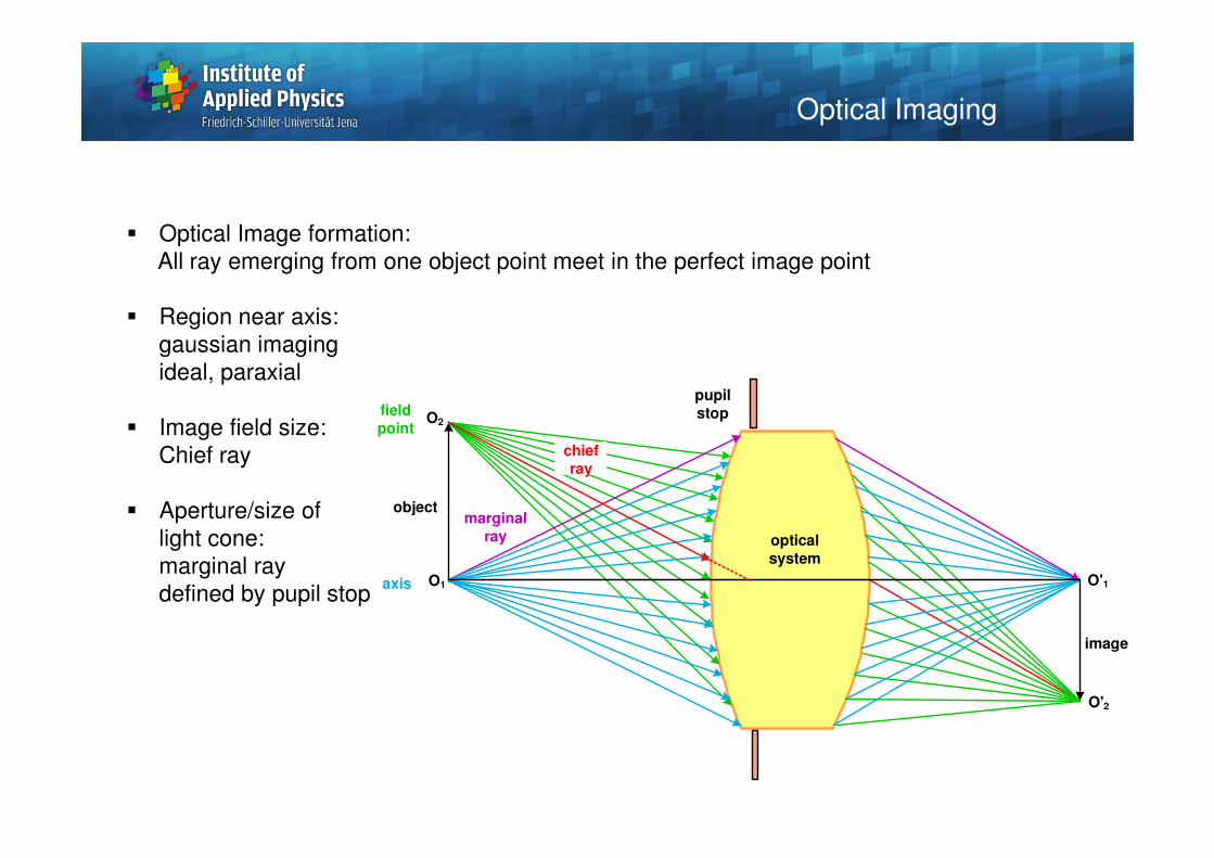
� Optical Image formation:

All ray emerging from one object point meet in the perfect image point

� Region near axis:

gaussian imaging

ideal, paraxial

� Image field size:

Chief ray

� Aperture/size of

light cone:

marginal ray

defined by pupil stop

Optical Imaging

image

object

optical

system

O2field

point

axis

pupil

stop

marginal

ray

O1 O'1

O'2

chiefray

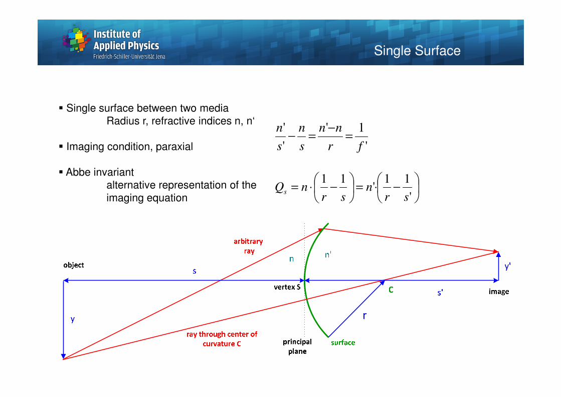
� Single surface between two media

Radius r, refractive indices n, n‘

� Imaging condition, paraxial

� Abbe invariant

alternative representation of the

imaging equation

'

1'

'

'

fr

nn

s

n

s

n=

−=−

−⋅=

−⋅=

'

11'

11

srn

srnQs

Single Surface

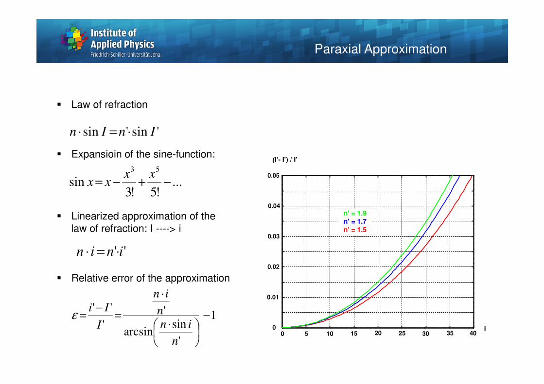
� Law of refraction

� Expansioin of the sine-function:

� Linearized approximation of the

law of refraction: I ----> i

� Relative error of the approximation

Paraxial Approximation

i0 5 10 15 20 25 30 35 40

0

0.01

0.02

0.03

0.04

0.05

((((i'- I') / I'

n' = 1.9

n' = 1.7

n' = 1.5

...!5!3

sin53

−+−=xx

xx

'sin'sin InIn ⋅=⋅

1

'

sinarcsin

'

'

''−

⋅

⋅

=−

=

n

inn

in

I

Iiε

'' inin ⋅=⋅

Linear Collineation

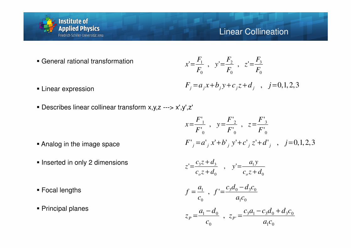
� General rational transformation

� Linear expression

� Describes linear collinear transform x,y,z ---> x',y',z'

� Analog in the image space

� Inserted in only 2 dimensions

� Focal lengths

� Principal planes

0

3

0

2

0

1 ',','F

Fz

F

Fy

F

Fx ===

3,2,1,0, =+++= jdzcybxaF jjjjj

0

3

0

2

0

1

'

',

'

',

'

'

F

Fz

F

Fy

F

Fx ===

3,2,1,0,'''''''' =+++= jdzcybxaF jjjjj

0

1

0

33 ','dzc

yay

dzc

dzcz

oo +=

+

+=

01

0303

0

1 ',ca

cddcf

c

af

−==

01

030313

'

0

01 ,ca

cddcacz

c

daz PP

+−=

−=

Linear Collineation

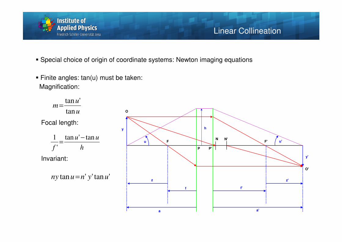
� Special choice of origin of coordinate systems: Newton imaging equations

� Finite angles: tan(u) must be taken:

Magnification:

Focal length:

Invariant:

O

O'

y'

y

F F'

P P'

N N'

f'

a'a

f

z'z

u'u

h

u

um

tan

'tan=

h

uu

f

tan'tan

'

1 −=

'tan''tan uynuny =

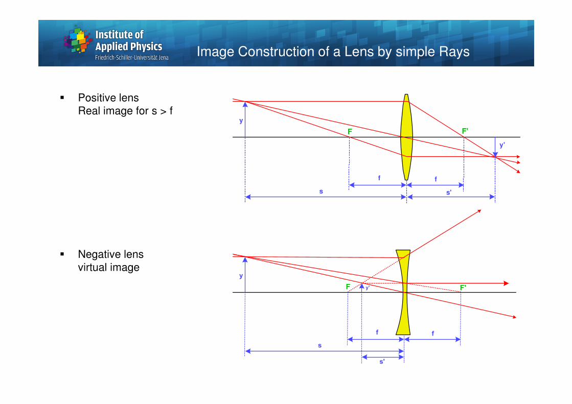
� Positive lens

Real image for s > f

� Negative lens

virtual image

F'F

y

f f

y'

s's

F'F

y

f f

y'

s'

s

Image Construction of a Lens by simple Rays

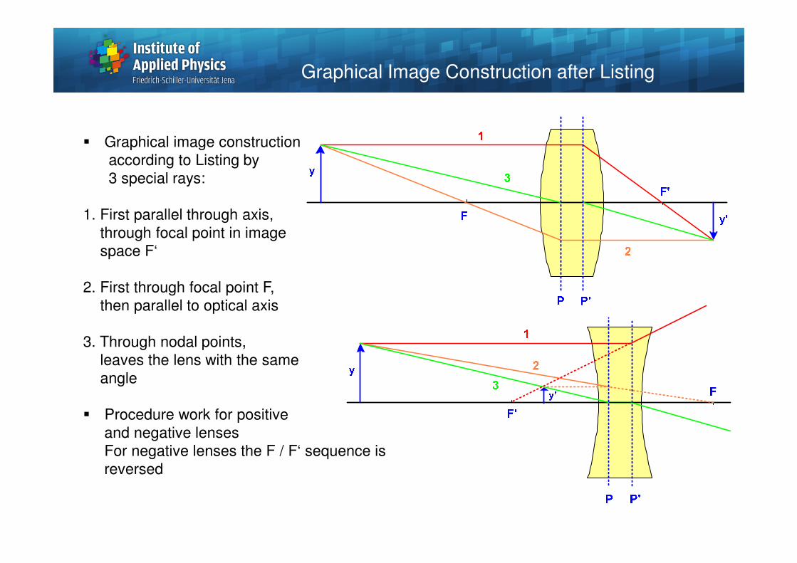
� Graphical image construction

according to Listing by

3 special rays:

1. First parallel through axis,

through focal point in image

space F‘

2. First through focal point F,

then parallel to optical axis

3. Through nodal points,

leaves the lens with the same

angle

� Procedure work for positive

and negative lenses

For negative lenses the F / F‘ sequence is

reversed

Graphical Image Construction after Listing

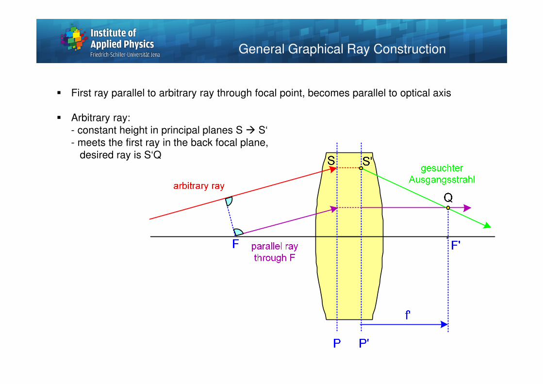
� First ray parallel to arbitrary ray through focal point, becomes parallel to optical axis

� Arbitrary ray:

- constant height in principal planes S � S‘

- meets the first ray in the back focal plane,

desired ray is S‘Q

General Graphical Ray Construction

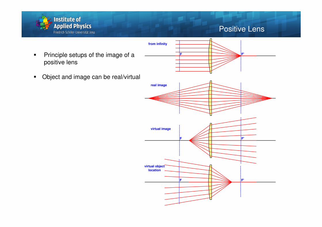
� Principle setups of the image of a

positive lens

� Object and image can be real/virtual

Positive Lens

from infinity

real image

virtual image

F F'

F'F

F'F

virtual objectlocation

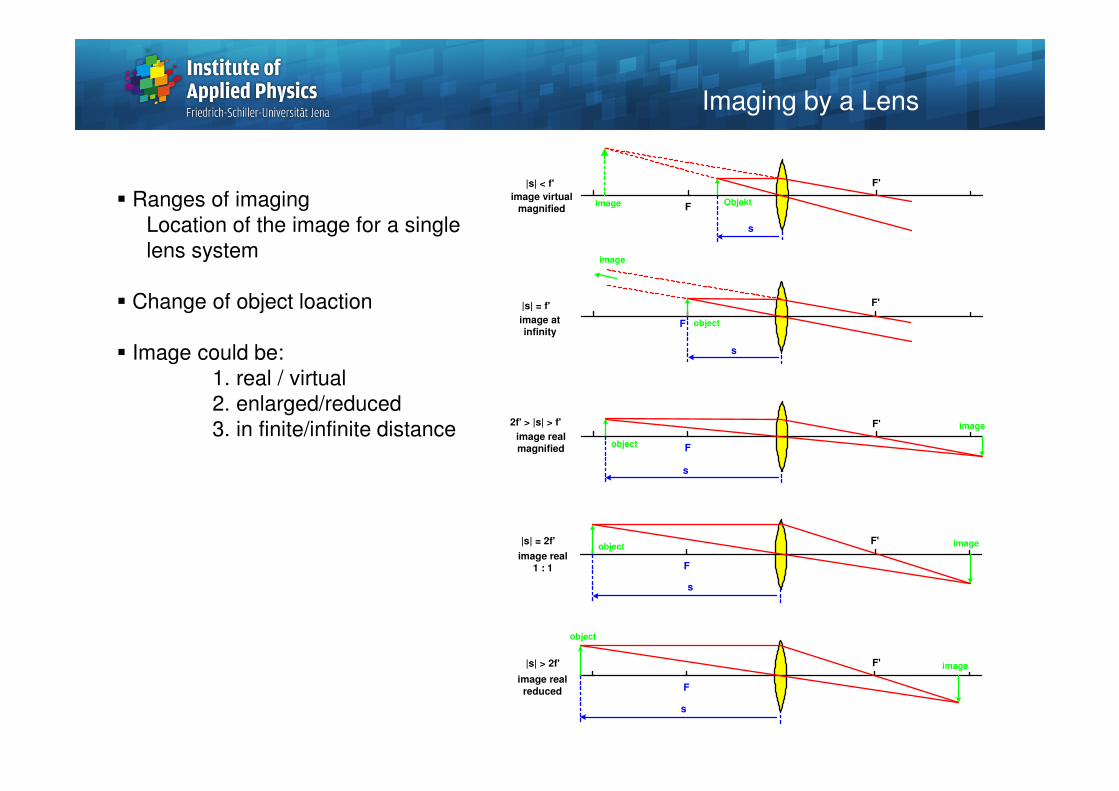
� Ranges of imaging

Location of the image for a single

lens system

� Change of object loaction

� Image could be:

1. real / virtual

2. enlarged/reduced

3. in finite/infinite distance

Imaging by a Lens

|s| < f'

image virtualmagnified F

Objekt

s

F object

s

Fobject

s

F

object

s

F'

F

object

image

s

|s| = f'

2f' > |s| > f'

|s| = 2f'

|s| > 2f'

F'

F'

F'

F'

image

image

image

image

image atinfinity

image realmagnified

image real1 : 1

image realreduced

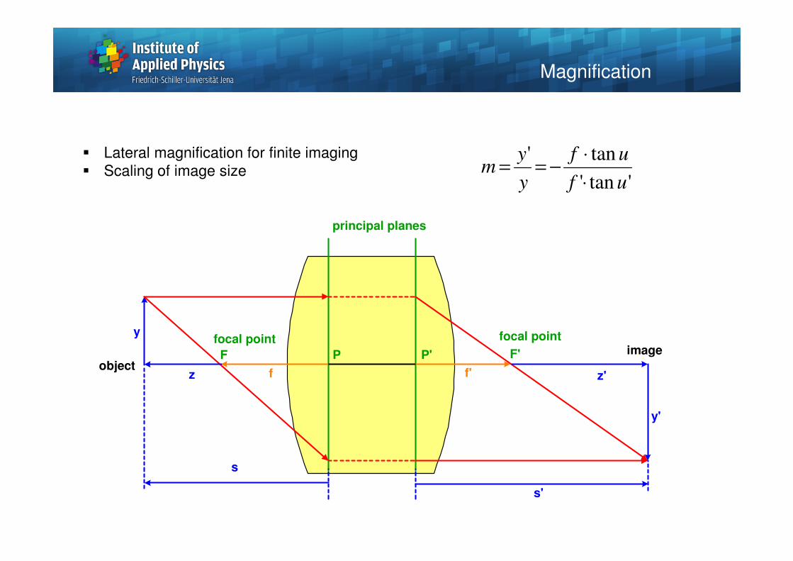
� Lateral magnification for finite imaging

� Scaling of image size'tan'

tan'

uf

uf

y

ym

⋅

⋅−==

Magnification

z f f' z'

y

P P'

principal planes

object

imagefocal pointfocal point

s

s'

y'

F F'

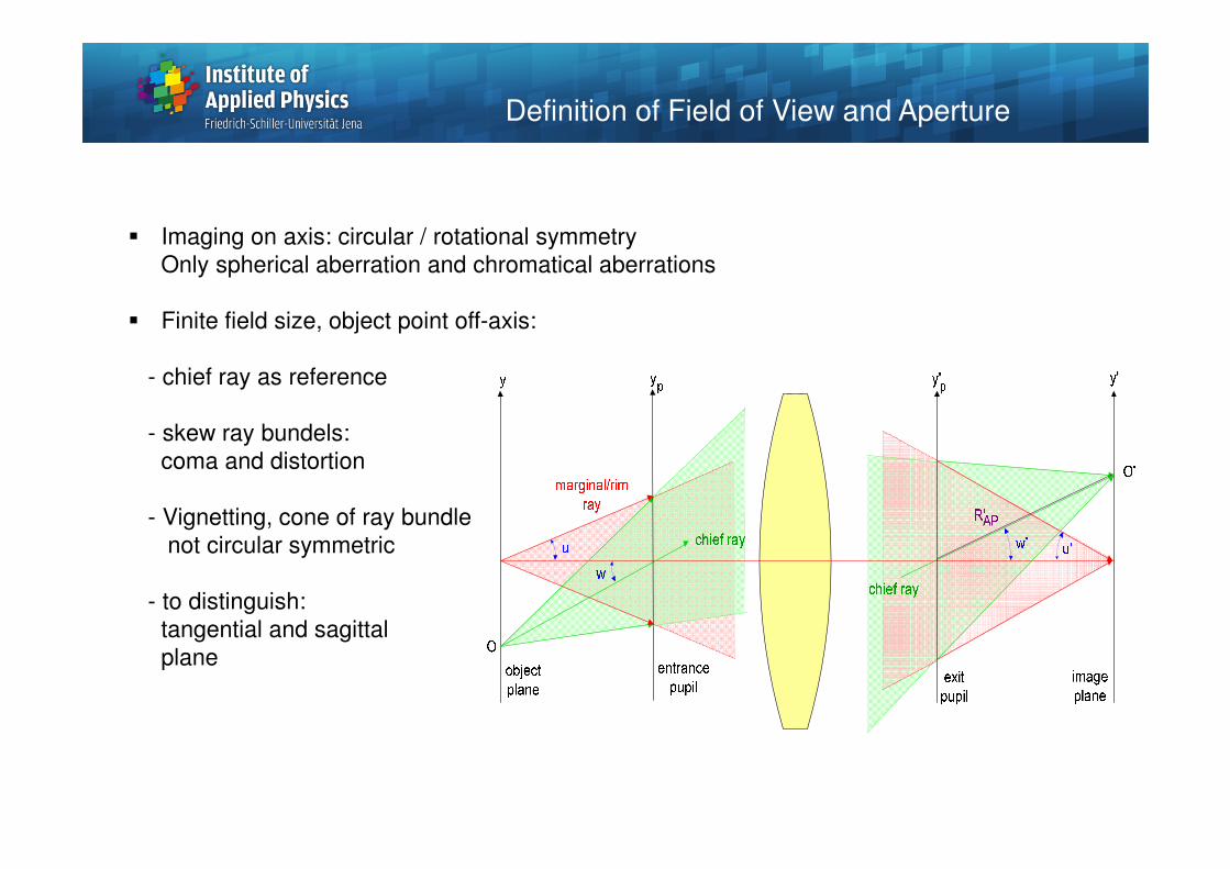
� Imaging on axis: circular / rotational symmetry

Only spherical aberration and chromatical aberrations

� Finite field size, object point off-axis:

- chief ray as reference

- skew ray bundels:

coma and distortion

- Vignetting, cone of ray bundle

not circular symmetric

- to distinguish:

tangential and sagittal

plane

Definition of Field of View and Aperture

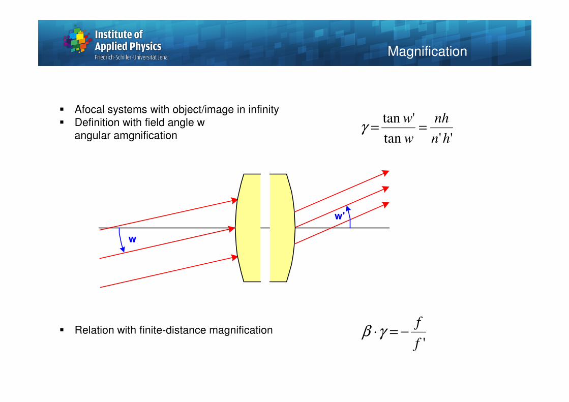
� Afocal systems with object/image in infinity

� Definition with field angle w

angular amgnification

� Relation with finite-distance magnification

''tan

'tan

hn

nh

w

w==γ

Magnification

w

w'

'f

f−=⋅γβ

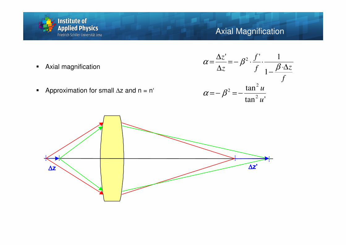
� Axial magnification

� Approximation for small ∆z and n = n‘

f

zf

f

z

z

∆⋅−

⋅⋅−=∆

∆=

ββα

1

1'' 2

'tan

tan2

2

2

u

u−=−= βα

Axial Magnification

∆∆∆∆z ∆∆∆∆z'

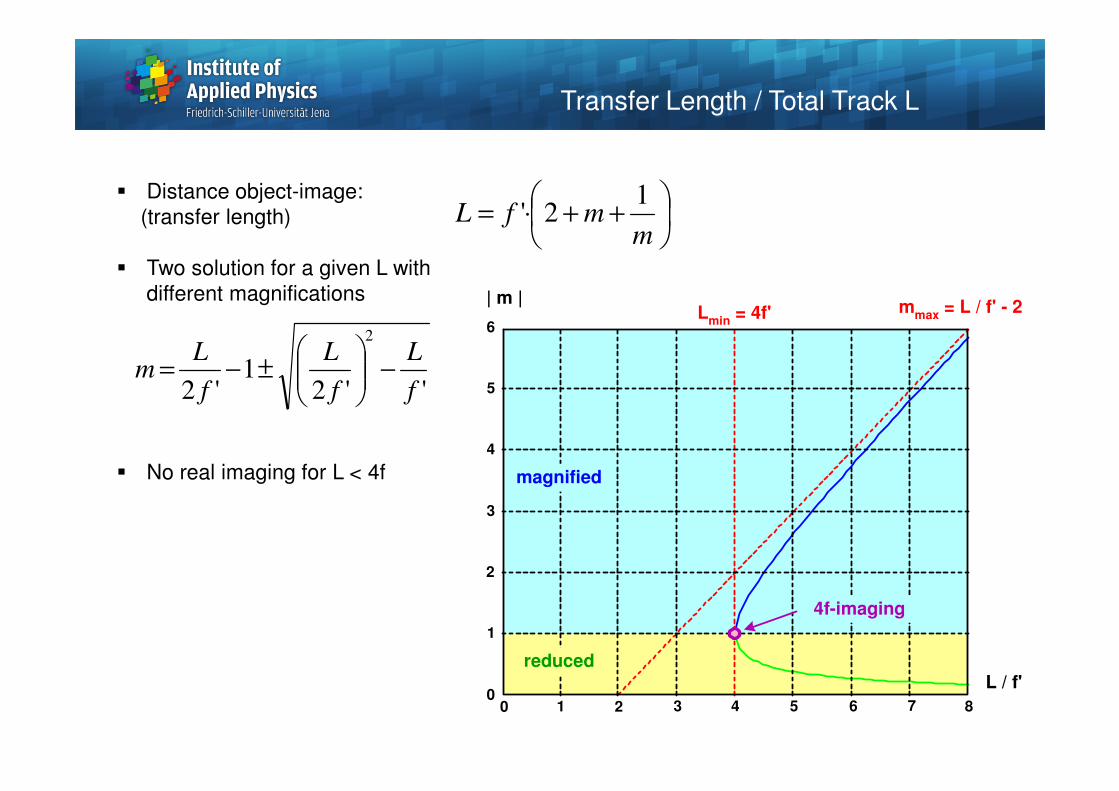
� Distance object-image:

(transfer length)

� Two solution for a given L with

different magnifications

� No real imaging for L < 4f

Transfer Length / Total Track L

++⋅=

mmfL

12'

''21

'2

2

f

L

f

L

f

Lm −

±−=

| m |

0 1 2 3 4 5 6 7 80

1

2

3

4

5

6

L / f'

magnified

reduced

Lmin

= 4f' mmax

= L / f' - 2

4f-imaging

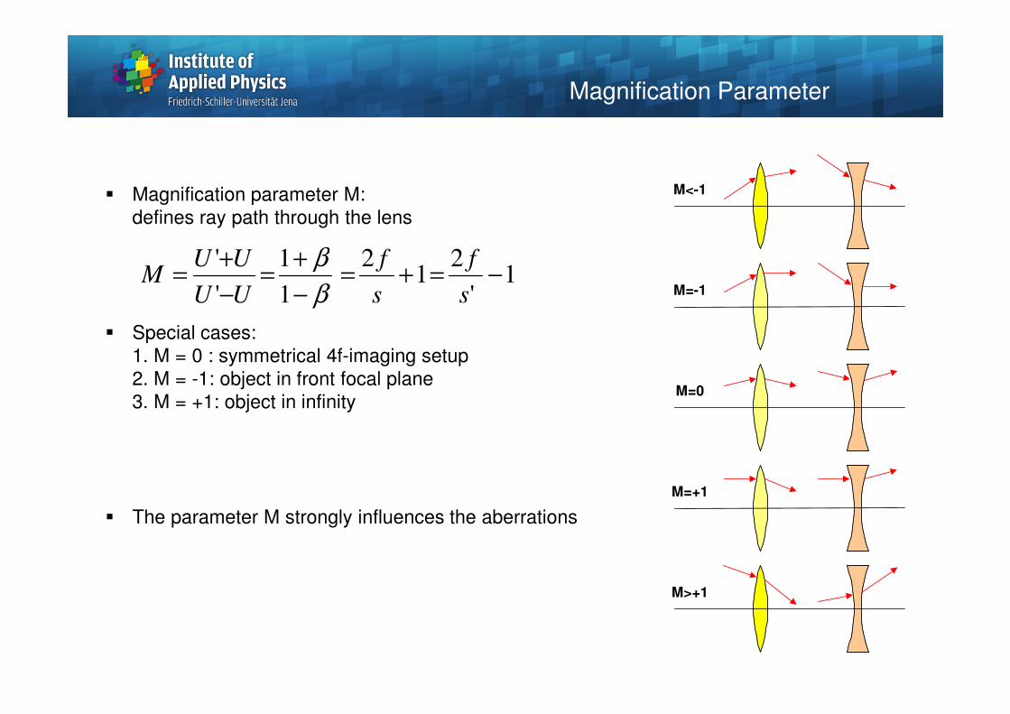
� Magnification parameter M:

defines ray path through the lens

� Special cases:

1. M = 0 : symmetrical 4f-imaging setup

2. M = -1: object in front focal plane

3. M = +1: object in infinity

� The parameter M strongly influences the aberrations

1'

21

2

1

1

'

'−=+=

−

+=

−

+=

s

f

s

f

UU

UUM

β

β

Magnification Parameter

M=0

M=-1

M<-1

M=+1

M>+1

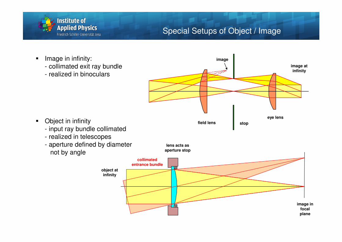
� Image in infinity:

- collimated exit ray bundle

- realized in binoculars

� Object in infinity

- input ray bundle collimated

- realized in telescopes

- aperture defined by diameter

not by angle

Special Setups of Object / Image

object atinfinity

image in

focalplane

lens acts as

aperture stop

collimatedentrance bundle

image atinfinity

stop

image

eye lens

field lens

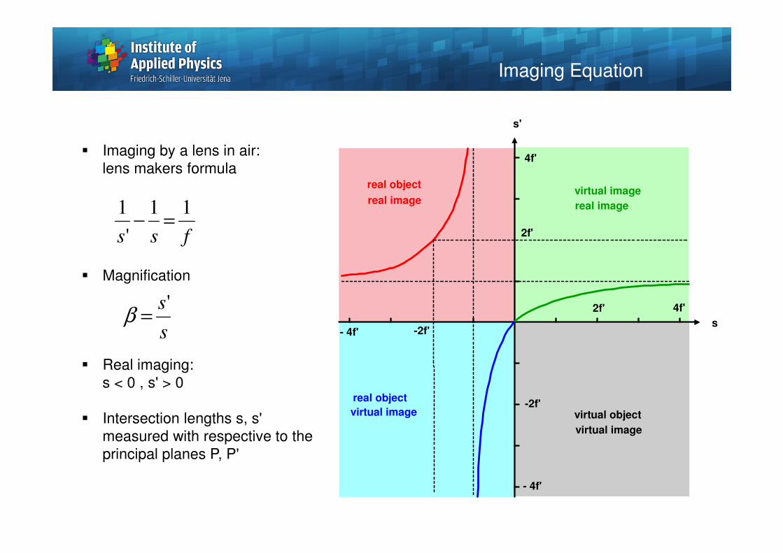
� Imaging by a lens in air:

lens makers formula

� Magnification

� Real imaging:

s < 0 , s' > 0

� Intersection lengths s, s'

measured with respective to the

principal planes P, P'

fss

11

'

1=−

s

s'=β

Imaging Equation

s'

2f'

4f'

2f' 4f'

s-2f'- 4f'

-2f'

- 4f'

real object

real image

real object

virtual object

virtual image

virtual image

real image

virtual image

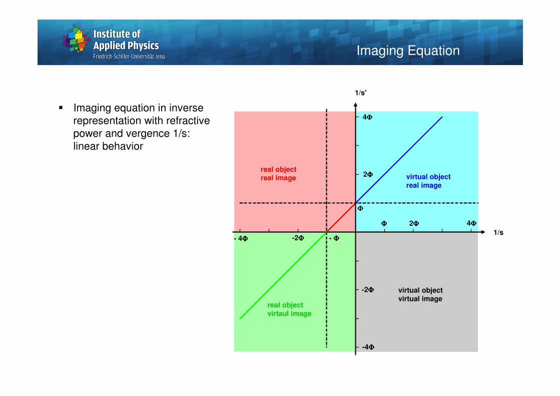
� Imaging equation in inverse

representation with refractive

power and vergence 1/s:

linear behavior

Imaging Equation

1/s'

2ΦΦΦΦ

4ΦΦΦΦ

2ΦΦΦΦ 4ΦΦΦΦ

1/s-2ΦΦΦΦ- 4ΦΦΦΦ

-2ΦΦΦΦ

-4ΦΦΦΦ

real objectreal image

real objectvirtaul image

virtual objectvirtual image

virtual objectreal image

ΦΦΦΦ

ΦΦΦΦ

- ΦΦΦΦ

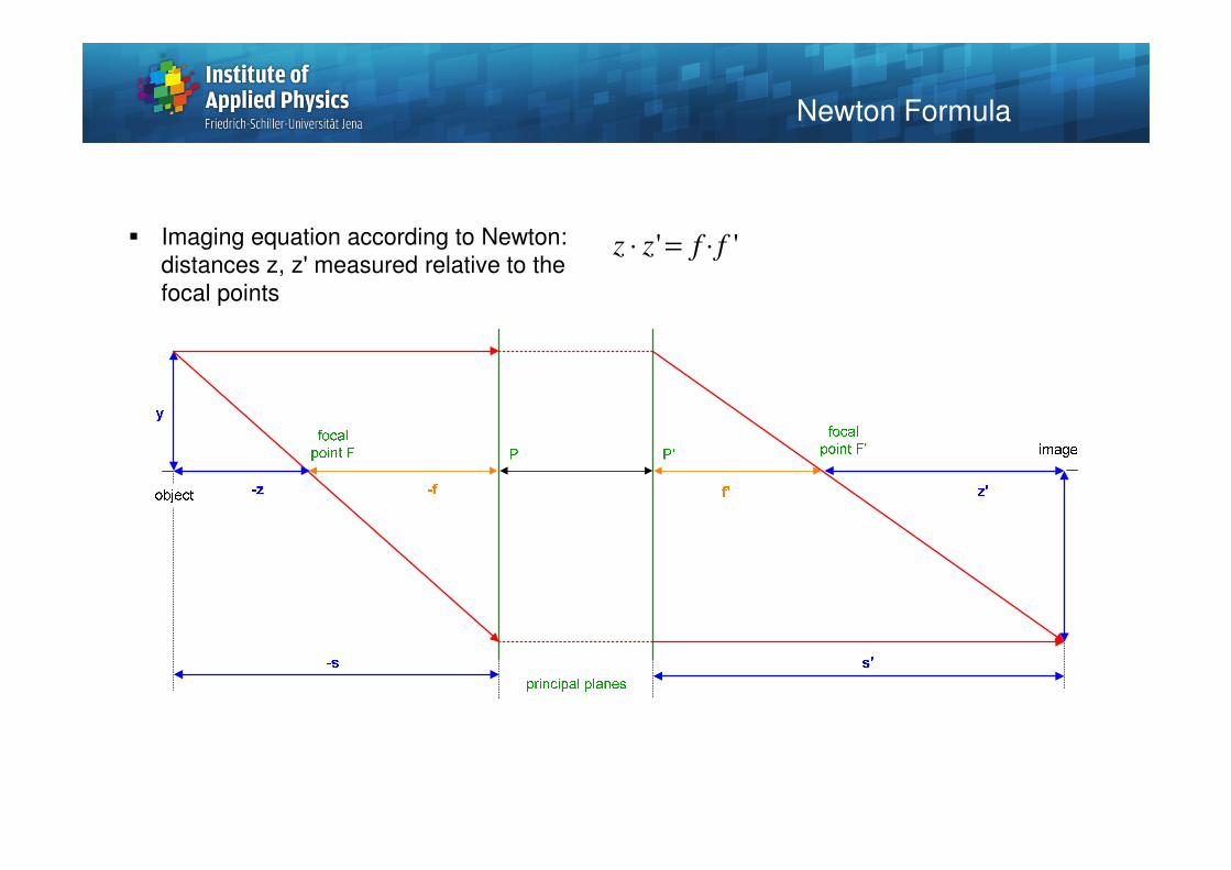
� Imaging equation according to Newton:

distances z, z' measured relative to the

focal points

'' ffzz ⋅=⋅

Newton Formula

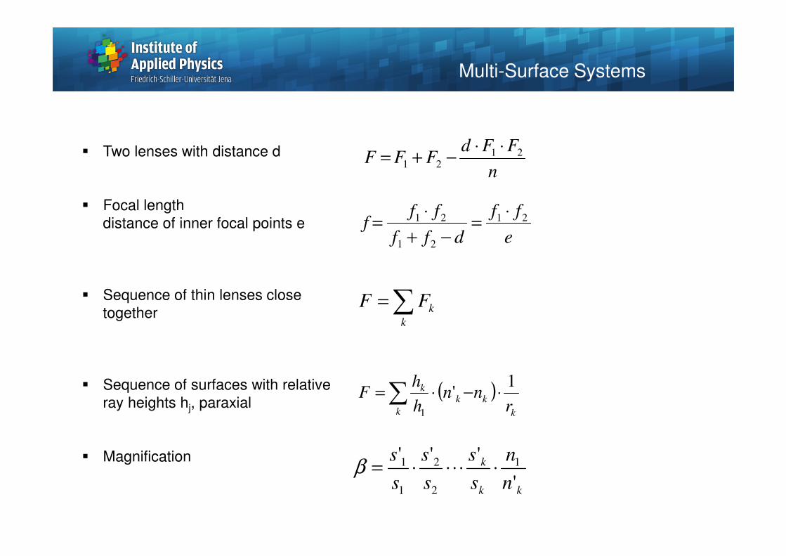
� Two lenses with distance d

� Focal length

distance of inner focal points e

� Sequence of thin lenses close

together

� Sequence of surfaces with relative

ray heights hj, paraxial

� Magnification

n

FFdFFF 21

21

⋅⋅−+=

e

ff

dff

fff 21

21

21⋅

=−+

⋅=

∑=k

kFF

( )∑ ⋅−⋅=k k

kkk

rnn

h

hF

1'

1

kk

k

n

n

s

s

s

s

s

s

'

''' 1

2

2

1

1 ⋅⋅⋅⋅⋅=β

Multi-Surface Systems

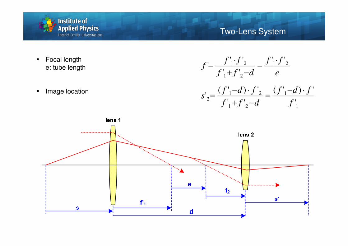
� Focal length

e: tube length

� Image location

Two-Lens System

e

ff

dff

fff 21

21

21 ''

''

'''

⋅=

−+

⋅=

1

1

21

21

2'

')'(

''

')'('

f

fdf

dff

fdfs

⋅−=

−+

⋅−=

Matrix Calculus

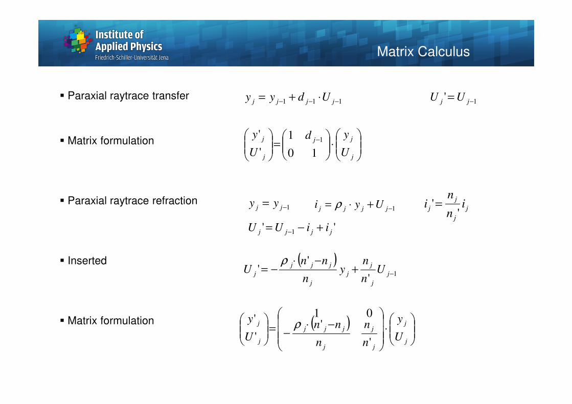
� Paraxial raytrace transfer

� Matrix formulation

� Paraxial raytrace refraction

� Inserted

� Matrix formulation

111 −−− ⋅+= jjjj Udyy

1−+⋅= jjjj Uyi ρ in

nij

j

j

j''

=

1' −= jj UU

1−= jj yy

( )1

'

'' −+

−⋅−= j

j

j

j

j

jjj

j Un

ny

n

nnU

ρ

'' 1 jjjj iiUU +−= −

⋅

=

−

j

jj

j

j

U

yd

U

y

10

1

'

'1

( )

⋅

−⋅

−=

j

j

j

j

j

jjj

j

j

U

y

n

n

n

nnU

y

'

'01

'

' ρ

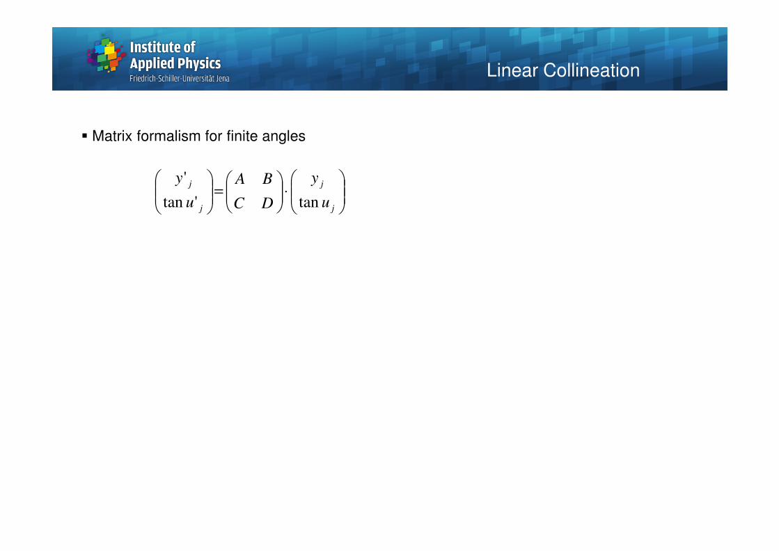
Linear Collineation

� Matrix formalism for finite angles

⋅

=

j

j

j

j

u

y

DC

BA

u

y

tan'tan

'

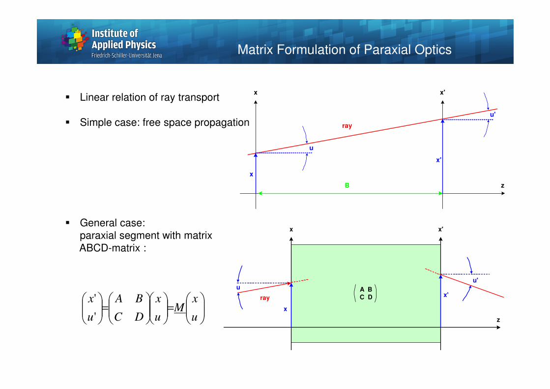
� Linear relation of ray transport

� Simple case: free space propagation

� General case:

paraxial segment with matrix

ABCD-matrix :

=

=

u

xM

u

x

DC

BA

u

x

'

'

z

x x'

ray

x'

u'

u

x

B

Matrix Formulation of Paraxial Optics

A B

C D

z

x x'

ray x'

u'u

x

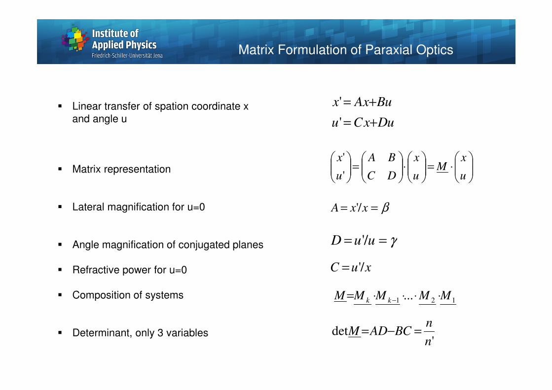
� Linear transfer of spation coordinate x

and angle u

� Matrix representation

� Lateral magnification for u=0

� Angle magnification of conjugated planes

� Refractive power for u=0

� Composition of systems

� Determinant, only 3 variables

uDxCu

uBxAx

+=

+=

'

'

⋅=

⋅

=

u

xM

u

x

DC

BA

u

x

'

'

β== xxA /'

γ== uuD /'

xuC /'=

121... MMMMM kk ⋅⋅⋅⋅= −

'det

n

nCBDAM =−=

Matrix Formulation of Paraxial Optics

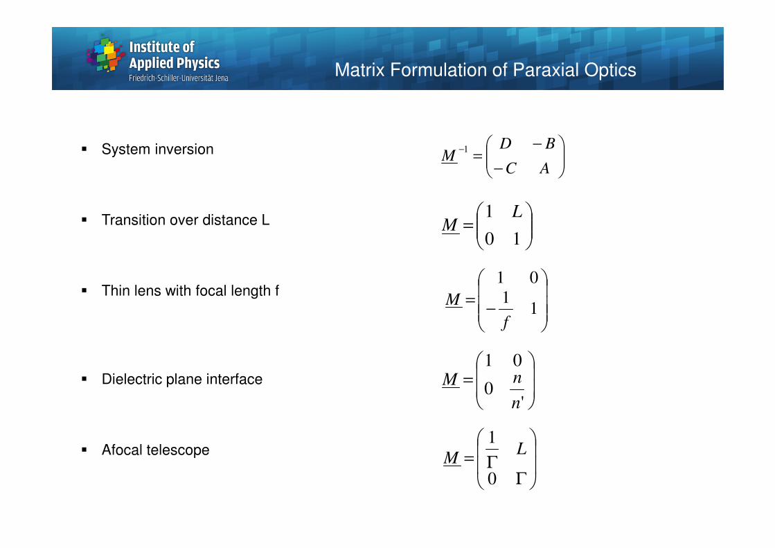
� System inversion

� Transition over distance L

� Thin lens with focal length f

� Dielectric plane interface

� Afocal telescope

−

−=

−

AC

BDM

1

=

10

1 LM

−=

11

01

f

M

=

'0

01

n

nM

ΓΓ=0

1L

M

Matrix Formulation of Paraxial Optics

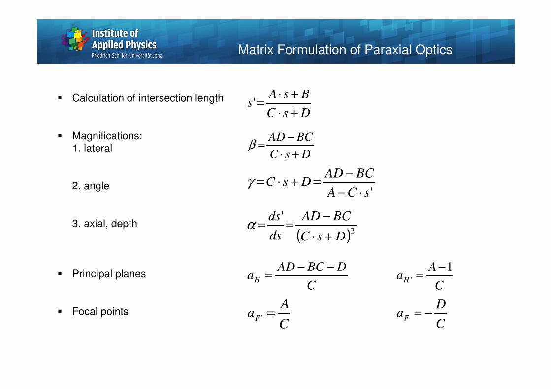
� Calculation of intersection length

� Magnifications:

1. lateral

2. angle

3. axial, depth

� Principal planes

� Focal points

Matrix Formulation of Paraxial Optics

DsC

BsAs

+⋅

+⋅='

DsC

BCAD

+⋅

−=β

( )2

'

DsC

BCAD

ds

ds

+⋅

−==α

'sCA

BCADDsC

⋅−

−=+⋅=γ

C

DBCADaH

−−=

C

AaH

1'

−=

C

AaF ='

C

DaF −=

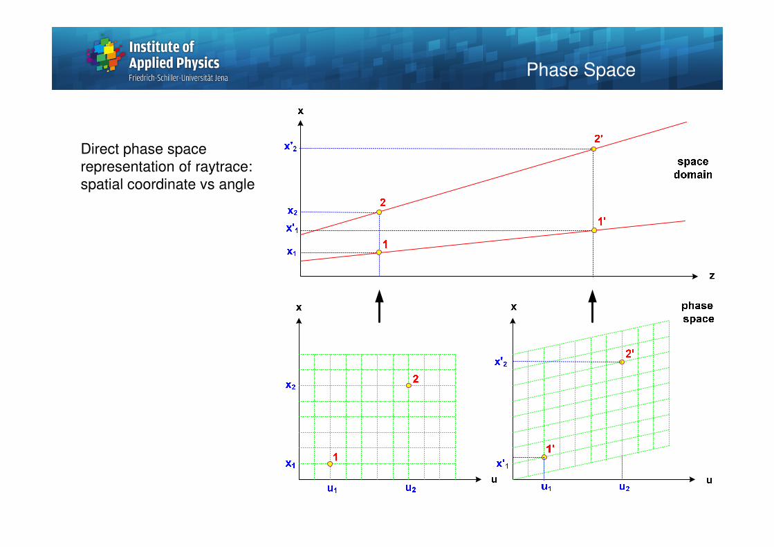
Direct phase space

representation of raytrace:

spatial coordinate vs angle

Phase Space

Phase Space

z

x

I

x

I

x

u

x

u

x

Phase Space

z

x

x

u

1

1

2 2'

2 2'

3 3' 4

33'

5

4

5

6

6

free

transfer

lens 1

lens 2

grin lens

lens 1

lens 2

free

transfer

free transfer

free transfer

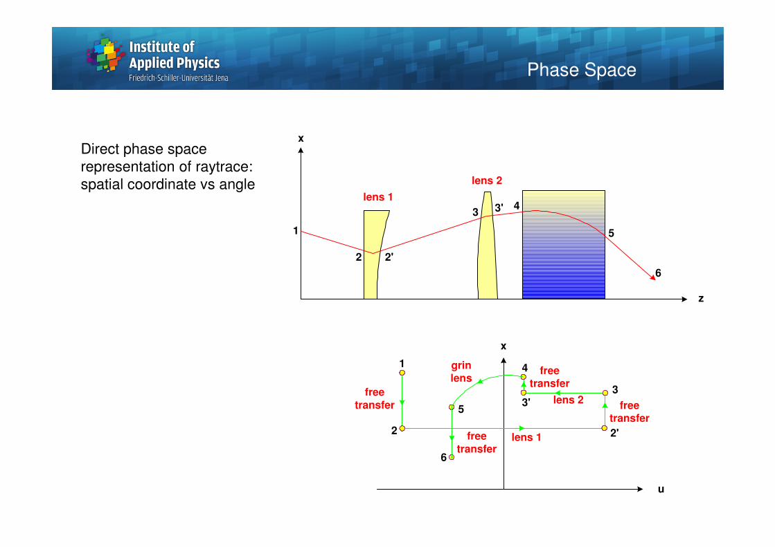
Direct phase space

representation of raytrace:

spatial coordinate vs angle

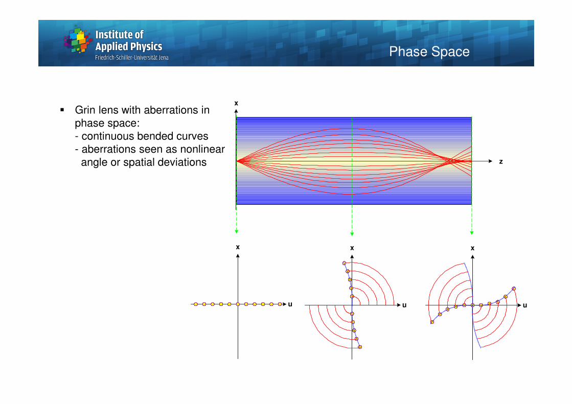
� Grin lens with aberrations in

phase space:

- continuous bended curves

- aberrations seen as nonlinear

angle or spatial deviations

Phase Space

z

x

x

u u

x

u

x

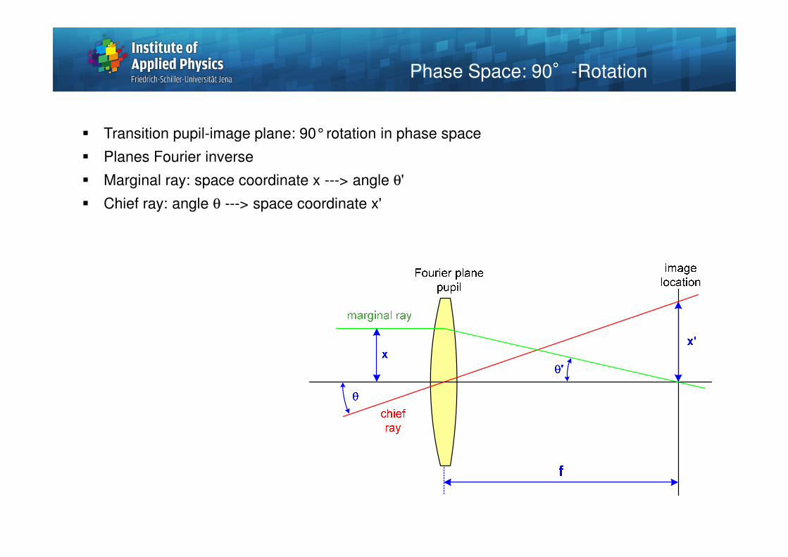
Phase Space: 90°-Rotation

� Transition pupil-image plane: 90°rotation in phase space

� Planes Fourier inverse

� Marginal ray: space coordinate x ---> angle θ'

� Chief ray: angle θ ---> space coordinate x'

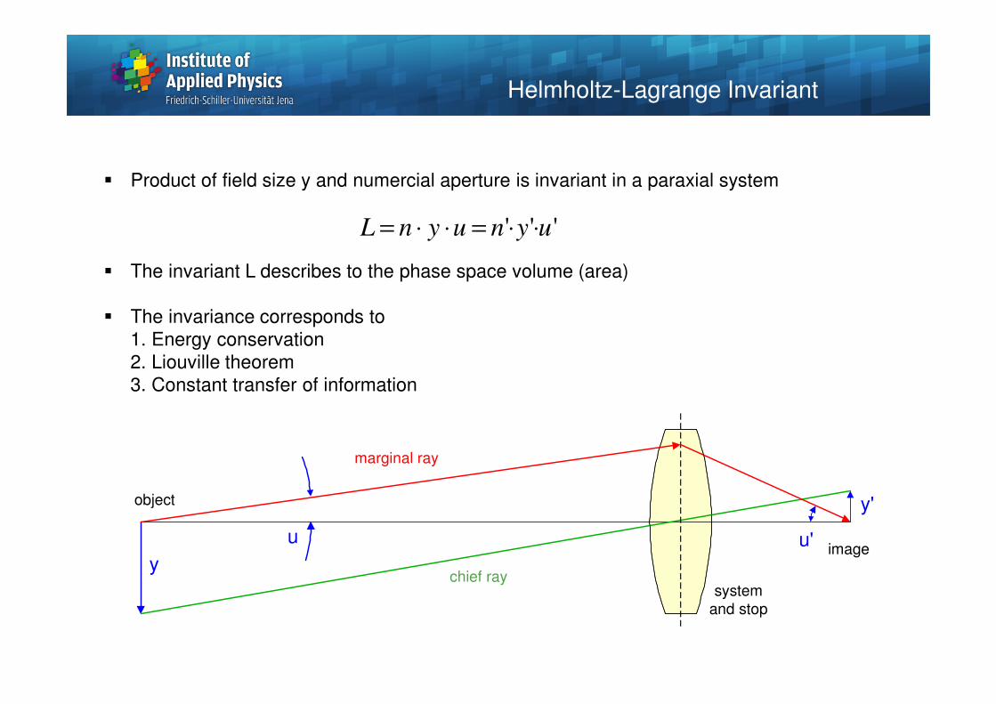
� Product of field size y and numercial aperture is invariant in a paraxial system

� The invariant L describes to the phase space volume (area)

� The invariance corresponds to

1. Energy conservation

2. Liouville theorem

3. Constant transfer of information

y

y'

u u'

marginal ray

chief ray

object

image

system

and stop

''' uynuynL ⋅⋅=⋅⋅=

Helmholtz-Lagrange Invariant

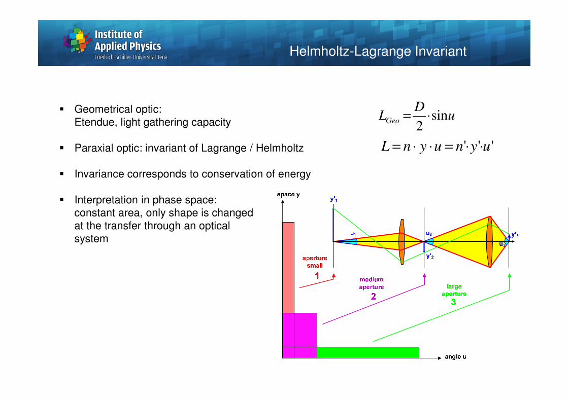
� Geometrical optic:

Etendue, light gathering capacity

� Paraxial optic: invariant of Lagrange / Helmholtz

� Invariance corresponds to conservation of energy

� Interpretation in phase space:

constant area, only shape is changed

at the transfer through an optical

system

uD

LGeo sin2

⋅=

''' uynuynL ⋅⋅=⋅⋅=

Helmholtz-Lagrange Invariant

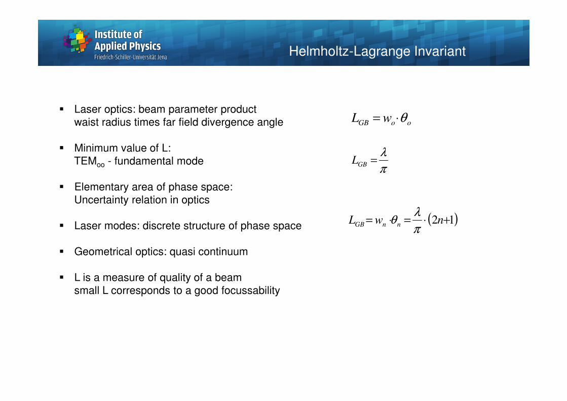
� Laser optics: beam parameter product

waist radius times far field divergence angle

� Minimum value of L:

TEMoo - fundamental mode

� Elementary area of phase space:

Uncertainty relation in optics

� Laser modes: discrete structure of phase space

� Geometrical optics: quasi continuum

� L is a measure of quality of a beam

small L corresponds to a good focussability

ooGB wL θ⋅=

π

λ=GBL

( )12 +⋅=⋅= nwL nnGBπ

λθ

Helmholtz-Lagrange Invariant

Summary of Important Topics

� Nonlinearity of the law of refraction defines the paraxial approximation

� Linera collineation: general approach of linear mapping, in case of larger angles with tan(u)

� Graphical image construction in paraxial optics:

3 rays determine location and size of the image: nodal ray, rays through focal points F, F‘

are parallel to axis

� Imaging condition of a single lens: real image for object distances s>2f , virtual images for

closer object points

� Definition of lateral magnification, angle and depth magnification

� Lens makers formula -1/s+1/s‘=1/f allows for paraxial imaging calculations

� Combination of several lenses, cascaded systems

For thin components near together: focal power F=1/f is additive

� Matrix calculus: practical calculation scheme with 2x2 ABCD matrices, connect ray

coordinate and angle between two planes

� Phase space in optics: spatial coordinate y and angle u

� Illustration of optical systems and ray paths by a line in the phase space

� Lagrange invariant: constant area of a ray bundle in phase space, corresponds to the

conservation of energy

40

Outlook

Next lecture: Part 5 – Properties of optical systems

Date: Wednesday, 2012-05-16

Content: 5.1 Pupil - basic notations

- pupil

- special rays

- vignetting

- ray sets

5.2 Special imaging setups - telecentricity

- anamorphotic imaging

- Scheimpflug condition

5.3 Canonical coordinates - normalized properties

- pupil sphere

5.4 Delano diagram - basic idea

- examples