Embed Size (px)
Citation preview

Design and Implementation of a Linear
Control System for a Two-wheeled vehicle
and a Robotic Bicycle
Alex Martinez
A thesis submitted in partial fulfillment
of the requirements for the degree of
BACHELOR OF APPLIED SCIENCE
Supervisor: Prof. Foued Ben Amara
Department of Mechanical and Industrial Engineering
University of Toronto
March 2008
Abstract
This thesis describes the design and the implementation of a linear control system
that is implemented in a two wheeled vehicle and a bicycle using LEGO NXT
Mindstorms ® motors and the included microcontroller (the so called “brick”). A
potentiometer is adapted to work as a tilt sensor and interfaced as a light sensor. A
state-space and observer are designed for both vehicles and are then implemented
in the programming language robotC. A neural network algorithm is proposed to
optimize the constants of the control system for the two wheeled vehicle.

i.
Acknowledgments
I thank Prof. Foued Ben Amara for his support and for being available for
consultation in short notice (by knocking on his office’s door).

ii.
1Introduction and Motivation ............................................................................................. 7
2 Project Description........................................................................................................... 8
3 Literature Review............................................................................................................. 9
4 Hardware design ............................................................................................................ 10
4.1 Tilt Sensor Design................................................................................................... 10
4.2 Two-wheeled Vehicle Design ................................................................................. 14
3 Bicycle Design ........................................................................................................... 15
5 Software design .............................................................................................................. 18
5.1 Tilt Sensor Calibration Program ............................................................................. 18
5.2 Motor Acceleration Calibration Program ............................................................... 20
5.3 State-space (PD Controller) Program for a Two-wheeled Vehicle ........................ 24
5.3.1 Derivation of a Linear Model for an Inverted Pendulum .................................... 24
5.3.1 State-space controller design ........................................................................... 26
5.3.2 Implementation in robotC Code....................................................................... 28
5.3.3 Addition of observer to the state-space controller ........................................... 28
5.3.4 Implementation in robotC Code....................................................................... 30
5.3.5 Addition of Neural Network Optimization for State-space Controller ............ 30
5.4 State-space (PD Controller) Program for a Bicycle ............................................ 31
5.4.1 Derivation of Linear Model for a Bicycle........................................................ 31
5.4.2 State-space controller design ........................................................................... 36
6 Future Work ................................................................................................................... 37
7 Conclusions .................................................................................................................... 37
References ......................................................................................................................... 38
Appendix A: Derivation of Non-linear Equations for a Bicycle ...................................... 39
Appendix D: robotC Code for Tilt Sensor Calibration Program ...................................... 48
Appendix E: robotC Code for Motor Acceleration Calibration Program ......................... 50
Appendix F: robotC Implementation of State-Space Controller for Two-Wheeled Vehicle
........................................................................................................................................... 52
Appendix G: robotC Implementation of State-Space Controller for Two-Wheeled Vehicle
with Observer .................................................................................................................... 54

iv.
List of Symbols

List of Figures
Figure 1: possible way of using light sensors instead of a tilt sensor while also
compensating for difference in readings due to different lighting conditions .................. 11
Figure 2: graph showing effect of the length of R2 on the derivative of theta 1 that is
inversely proportional to error “amplification” ................................................................ 12
Figure 3: front and back views of the two-wheeled vehicle ............................................. 14
Figure 4: Two-wheeled vehicle being balanced by a PD controller with observer .......... 15
Figure 5: the robotic bicycle ............................................................................................. 16
Figure 6: structural details of robotic bicycle ................................................................... 16
Figure 7: front wheel assembly ......................................................................................... 17
Figure 8: back wheel assembly ......................................................................................... 17
Figure 9: detail showing tilt sensor attachment point and the use of a rod from the NXT ®
kit to stop the tilt sensor rod from moving backwards when operating ............................ 17
Figure 10: relationship between lightSensor value and angle showing a linear relationship
except for angles greater than 110 or smaller than around 60 degrees ............................. 19
Figure 11: linear relationship for a smaller range of angles with an acceptable error ...... 19
Figure 12: typical response of a motor model taking into account emf and inertia to a step
voltage input...................................................................................................................... 21
Figure 13: velocity profile measured from the motors after backward difference
differentiation performed on measurements done in the brick ......................................... 22
Figure 14: acceleration profile after using backward difference to differentiate calculated
velocity values. This method cannot be used since initial acceleration is not known. The
value 0.01 is an estimation ................................................................................................ 22
Figure 15: transform performed on calculated velocity values to determine motor model
constants used to determine the initial acceleration .......................................................... 23
Figure 16: relationship between initial angular acceleration and power level .................. 24
Figure 17: inverted pendulum coordinate system ............................................................. 25
Figure 18: SIMULINK model of inverted pendulum ....................................................... 26
Figure 19: output of scope ................................................................................................ 27
Figure 20: SIMULINK model of inverted pendulum with PD controller ........................ 27
Figure 21: output of scope ................................................................................................ 28
Figure 22: SIMULINK model of inverted pendulum with PD controller and observer ... 29
Figure 23: output of scope ................................................................................................ 30
Figure 24: point-mass model of bicycle on left-handed coordinate system ..................... 31
Figure 25: front view of bicycle with coordinate system ................................................. 32
Figure 26: top view of bicycle and coordinate system ..................................................... 34
Figure 27: relationships between point accelerations and distance from the rotating point
P1 ...................................................................................................................................... 35
Figure 28: the rotation of the front wheel changes the direction of vector V producing the
new vector V with equal magnitude ............................................................................... 36
Figure 29: Point-mass model of bicycle on left-handed coordinate system. Notice the use
of an absolute coordinate system. The intersection between the x axis and the line made

by the two contact points doesn’t have to be at the origin. Also angles and are in the
z-x plane. ........................................................................................................................... 39
Figure 30: top view of the bicycle .................................................................................... 40
Figure 31: 3D shape resulting from the intersection of the planes intersecting the back
wheel, the front wheel, the ground and a plane perpendicular to the ground ................... 42
Figure 32 ........................................................................................................................... 45


1Introduction and Motivation
The purpose of this thesis is to make a suitable controller for both a two wheeled
vehicle and a bicycle built using the LEGO NXT Mindstorms ® kit. A state-space
controller equal to a PD controller will be designed and implemented for the two-wheeled
vehicle and the robotic-bicycle. The values from the design will be used as a first
estimate to the values needed in the software implementation. The values were changed
by trial and error to yield satisfactory controllers. A similar procedure was carried out for
the design and implementation of observers. An observer yields better results than taking
the derivative of the input because the observer carries out integration instead of a
derivation, acting as a low pass filter. Then a learning algorithm is described that can be
used to optimize the values of the controllers even further but it requires a functioning
control system to start with.
The steps of the controller design process used and suggested by this thesis are:
Find approximate values for the gains for a PD controller using a linearization
about the operating point using linear equations of the system
Design software to measure inputs and outputs; finding the relationship between
motor acceleration and the corresponding input in the program
Adjust the gains in the software implementation to come up with a more robust
controller
Use a learning algorithm to optimize the gains even further

2 Project Description
To demonstrate the design procedure stated in chapter 1, A two-wheeled vehicle
has been built. The two wheeled vehicle is shown in section 4.2. It is modeled as an
inverted pendulum. A tilt sensor was designed using a potentiometer and software was
designed to measure the relationship between the light sensor output (the potentiometer
voltage output; an analog voltage input in the program is taken as a light sensor input)
and the corresponding angle. The relationship theoretically and experimentally (within a
certain range of angles centered about the operating point is shown to be linear. Then a
program was designed and implemented to measure the initial acceleration of the motors
given a certain power level given to the motors by the program (from -100 to 100). The
program takes a number of readings to determine the power level per angular acceleration
of the motors. The relationship is shown theoretically and experimentally to be of the
form y = kx. Based on the inverted pendulum model and the calibration software, a PD
controller is designed using state-space methods and its implemented in software. Then
an observer is designed and added to the program. The values of the controller are
adjusted to yield a better performing controller. The same procedure is carried out for the
robotic bicycle. Then a learning algorithm based on neural network learning algorithms is
derived and suggested as a way of optimizing the controller values.

3 Literature Review
[1] describes the derivation of non-linear and linear equations of a bicycle. These
equations were used to check the validity of the derivations carried out in this thesis in
sections 5.4.1 and Appendix A. [5] describes a derivation of the linear equations of a
bicycle taking into account all moments of inertia and the geometry of a real bicycle. The
equations are used to check the stability of a bicycle over different speeds and they show
a transition speed were the rider does not have to actively control the bicycle. This is also
the conclusion of a much simpler model in [3] that also demonstrates in simple terms that
this is due to the rake angle. It is the most comprehensive analysis of bicycle stability
done so far. [13] is a impressive PhD thesis showing how to control a simple model of a
non-linear point mass bicycle model by using inversion of non-linear maps; a relatively
new control method. The nonlinear equation derived for a bicycle in [13] is also used to
check the same equation derived in Appendix A. [12] applies the resulting nonlinear
controller found in [13] but they include the rake angle of the bicycle and the moment of
inertia of the front steering mechanism including the wheel. They used this controller for
a robotic motorcycle that participated in the DARPA grand challenge. It is by far the
most sophisticated control system for a bicycle implemented so far. [16] describes a
simpler but also reliable method of controlling a full size bicycle. The same approach is
used in this thesis.

4 Hardware design
The hardware for this thesis was designed mostly with in the LEGO Mindstorms
NXT ® kit. A 50k potentiometer and a 10k resistor was also used for a tilt sensor. A
60cm wooden stick was also used for the tilt sensor.
4.1 Tilt Sensor Design
The design of the tilt sensor was based on the following general design
constraints: low price, simplicity of the hardware so that is it reliable and robustness to
outside conditions. A gyroscopic sensor was not used because of price. The visible light
sensor found in the LEGO Mindstorms NXT ® is cheap (it is included in the kit) and it
has been used in other implementations of the design in [14] but if used as a tilt sensor by
trying to measure the distance of the sensor to the ground, the output is both dependent
on distance to the ground and the reflective properties of the ground. A possible solution
for this could be to use two sensors and place them as shown below to account for the
reflective properties of the ground. This thesis was used to check the

Figure 1: possible way of using light sensors instead of a tilt sensor while also compensating for
difference in readings due to different lighting conditions
Another novel method of measuring the angle between the ground and the robotic
bicycle is to use a rod connected to a variable resistor. This solution meets all the design
constraints and it is less sensitive to outside conditions. The setup is shown in Fig 1 of
Appendix C.
In Appendix C the relationship between angles 1 (angle between the bicycle and
the ground) and 3 (the angle between the rod and the bicycle) for position, velocity and
acceleration was determined. As shown in the equations, they are also in terms of 2R . Is
there any distance for 2R in terms of 1R that can make the sensor the least susceptible to
errors from measuring 3 ? A measure for this is the derivative of equation 2 in Appendix
C with respect to 3 . This is shown below. So the higher the derivative is, the error in
finding 1 will decrease. Subjectively, the error will decrease the longer 2R is. To find

the highest derivative from the derivative of equation 2 by evaluating it from 12 RR to
2R ( 12 200 RR ) equation 2 from Appendix C should be only dependant on 2R .
This is done by realizing that the operating point of the robot is close to 901 and
therefore: 12
1
3 /cos RR . By substituting this relation into equation 2, letting 11R
( 2R is in terms of 1R ) and deriving it the maximum derivative can be found as done
below.
Derivative of Theta 1 w.r.t Theta 3 @ Theta 1 = 0
0.1
0.2
0.3
0.4
0.5
0.6
0.7
0.8
0.9
1.0
10 20 30 40 50 60 70 80 90 100 110 120 130 140 150 160 170 180 190 200
Lengh of R2
De
riva
tive
Figure 2: graph showing effect of the length of R2 on the derivative of theta 1 that is inversely
proportional to error “amplification”
As expected, the longer the distance of the rod is, the lower the error is. For weight
reasons and concerns about the harmonic frequency of the rod (a thick wire) causing
unwanted errors, the distance chosen is 40cm. Due to a nonfunctioning function in the
robotC programming language (the atan() function). The equations in Appendix C can’t

be used in the software implementation. The angle reading can be used directly if the
ratio of R1 to R2 is low enough (as shown in equation 2 of Appendix C, 31 if the
ratio is 0) and if the angles remain close to an operating range. The operating range is
determined experimentally.

4.2 Two-wheeled Vehicle Design
The two-wheeled vehicle consists of two motors from the LEGO Mindstorms
NXT ® kit pieces to connect the two motors side by side and straight pieces used to
connect the brick to the motors at a sufficient height. At first the center of gravity was at
0.155 m from the ground but to increase the performance of the controller the center
gravity was raised to 0.24 m. A straight piece is used between the motors to attach the tilt
sensor. The final design is shown in fig 3. The design in operation is shown in fig 4.
Figure 3: front and back views of the two-wheeled vehicle

Figure 4: Two-wheeled vehicle being balanced by a PD controller with observer
3 Bicycle Design
The bicycle was designed to have the biggest dimensions possible (dimensions a,
b and h; check section 5.4.1) in order to increase controller performance while keeping
the weight and the number of pieces used to the ones available in one LEGO Mindstorms
NXT kit. A rod had to be attached on the opposite side of the tilt sensor attachment point
to stop the tilt sensor from moving backwards when the bicycle is moving. The front and
back wheel assemblies shown in figs 7 and 8 were designed to reduce the number of
pieces used.

Figure 5: the robotic bicycle
Figure 6: structural details of robotic bicycle

Figure 7: front wheel assembly
Figure 8: back wheel assembly
Figure 9: detail showing tilt sensor attachment point and the use of a rod from the NXT ® kit to stop
the tilt sensor rod from moving backwards when operating

5 Software design
The software design was carried out using the robotC programming language and
compiler from Robotics Academy with the intellectual property of Carnegie Mellon
University.
5.1 Tilt Sensor Calibration Program
The tilt sensor calibration program takes a reading of the light sensor input (the
potentiometer) at fixed angles shown in the brick’s LCD display. When the next angle is
reached by moving the wooden rod connected to the potentiometer, measuring the angle
using a semicircle, any button on the brick can be pressed to record the next angle. After
all angles are recorded the program performs a least square fit to come up with the a1 and
a0 of the following equation:
angle in degrees = lightSensor value * a1 + a0
The lightSensor value is the value stored in the program from the voltage reading
from the potentiometer. As shown in fig 10, if a big enough range of angles is sampled
then there are going to be errors in the calculation due to edge effects from the
potentiometer. Since the potentiometer won’t perform over such a range of angles the
range was decreased until a satisfactory range was found taking into account the R^2
value of the linear relationship. After some experimentation a satisfactory sampling range
ad interval was found to be 50-120 degrees using 10 degree intervals. The relationship
should be linear since if the voltage v_o is proportional to x (a position in the
potentiometer and its total length is L) and if the value of the POT is 50k ohms with a
current limiting resistor of 10k ohms then v_o is given by:

L
xvo
5010
5
Which is linearly proportional to x and since the lightSensor value is linearly proportional
to v_o then x is linearly proportional to the lightSensor value.
lightSensor value vs. angle
0
20
40
60
80
100
120
140
840 850 860 870 880 890 900 910 920 930
lightSensor value
an
gle
(d
eg
ree
s)
Figure 10: relationship between lightSensor value and angle showing a linear relationship except for
angles greater than 110 or smaller than around 60 degrees
lightSensor value vs. angle
y = -0.5735x + 533.35
0
20
40
60
80
100
120
140
700 720 740 760 780 800 820 840 860
lightSenssor value
an
gle
(d
eg
rees)
Figure 11: linear relationship for a smaller range of angles with an acceptable error

5.2 Motor Acceleration Calibration Program

As shown in [11], the transfer function of a motor model that takes into account
back emf and the polar inertia of its axle and a wheel or steering mechanism is of the
form:
1s
K
V
Finding the inverse Laplace transform with zero initial conditions and a step
voltage input yields:
tKeK
The derivative of the above function with respect to time yields the acceleration:
teK
The graphs of both equations are given in fig 12. Therefore the initial acceleration is
given by K . If it is assumed that the motors will be always running at a speed close to
zero we can assume that the power level given to the motors is proportional to initial
acceleration of the motors.
Typical motor velocity and acceleration response after step
voltage
0
2
4
6
8
10
12
0 2 4 6 8 10 12 14 16
time
an
gu
lar
sp
eed
velocity acceleration
Figure 12: typical response of a motor model taking into account emf and inertia to a step voltage
input

The velocity profile in fig 13 was obtained from data measured and calculated by the
brick and it shown a good agreement with the theoretical response. Unfortunately there is
no way of using a backward difference to get an initial acceleration since the acceleration
at t=0 is not zero. Also the error of doing two backwards differences becomes large as
shown in fig. 14.
Motor velocity response after step voltage
(from backward difference)
0
0.1
0.2
0.3
0.4
0.5
0.6
0.7
0.8
0 50 100 150 200 250 300 350
time (milliseconds)
an
gu
lar
velo
cit
y
(deg
rees/m
illi
seco
nd
)
Figure 13: velocity profile measured from the motors after backward difference differentiation
performed on measurements done in the brick
Motor acceleration response after step voltage
(from backward difference)
0
0.002
0.004
0.006
0.008
0.01
0.012
0 50 100 150 200 250 300 350 400
time (milliseconds)
an
gu
lar
accele
rati
on
(deg
rees/m
s^
2)
Figure 14: acceleration profile after using backward difference to differentiate calculated velocity
values. This method cannot be used since initial acceleration is not known. The value 0.01 is an
estimation

Therefore we have to find a way of finding the constants in the velocity response
equation and then multiplying them to get the initial acceleration. In order to use the least
squares method found in [17] we have to transform the measurements using the following
formula:
ii tKy lnln
Where: 0a and 1
0
a
eK
a
Unfortunately the value of K (the steady state velocity) has to be known
beforehand to apply this transformation. What can be done is to take the last 3 calculated
velocity measurements and assume that they are the steady state speed. After the
transformation is done using that assumption the resulting relationship is linear as shown
in fig. 15. Therefore the transformation can be used in the program. The program uses
backwards-difference differentiation and the transform mentioned to find the initial speed
for various power levels.
Transforming measured variables to apply least squares error
formulas
y = 0.0091x R2 = 0.9649
0
0.5
1
1.5
2
2.5
3
0 50 100 150 200 250 300 350
time (milliseconds)
tran
sfo
rmed
velo
cit
ies
(un
itle
ss)
Figure 15: transform performed on calculated velocity values to determine motor model constants
used to determine the initial acceleration

Then it finds the least squares fit assuming that 0 power level yields 0 initial acceleration
(a_o = 0). The modified least squares method is in the program and it is derived by
following the derivation given in [17] for the least squares error formulas. The
relationship is graphed below in fig. 16.
Determination of "moment of inertia" variable
y = 0.6518x R2 = 0.9568
0
20
40
60
80
100
120
0 20 40 60 80 100 120 140 160
initial angular acceleration (rads/sec^2)
po
wer
level
Figure 16: relationship between initial angular acceleration and power level
5.3 State-space (PD Controller) Program for a Two-wheeled Vehicle
5.3.1 Derivation of a Linear Model for an Inverted Pendulum
We start by taking the moment about he origin as shown in Fig 2:
TmghJ sin (1)
Linearizing about 0 , making J equal to 2mh by the definition of polar moment of
inertia and replacing T by hF since all the forces in this model are inertial and therefore
will act only on the mass:

ThFmghmh 2 (2)
To keep the signs consistent, a positive force will cause the positive moment shown in
Fig 18.
Figure 17: inverted pendulum coordinate system
In an inertial frame of reference the total force on the mass will be given by:
bT maF (3)
Where ba is an acceleration given to the base.
Equating (2) into (3) yields:
bhmamghmh 2

5.3.1 State-space controller design
The state space equations of the inverted pendulum are:
bahhg 1
0
0
10
01y
The characteristic equation with full state-space feedback is given by:
22122 2)(det nnh
gK
h
KBKAI
For a settling time of 0.8 seconds and an overshoot of 5%:
7.0 (from graph in [11])
2.88.07.0
6.4n
Therefore: 2.201K and 8.12K
Figs 18 and 19 are from a simulation in SIMULINK for the linear model without
a controller and figs 20 and 20 are from a simulation with the designed controller
Figure 18: SIMULINK model of inverted pendulum

Figure 19: output of scope
Figure 20: SIMULINK model of inverted pendulum with PD controller

Figure 21: output of scope
5.3.2 Implementation in robotC Code
The implementation in robotC code of the above controller uses the K values
found as an initial guess of the values needed in the setup
5.3.3 Addition of observer to the state-space controller
An observer is used to estimate states that might not be available for direct
measurement. From [7], the observer directly connected for feedback is:
LyxLCBKAx
xkab
It is proved in [7] that xx
as t but the settling time given by the following
equation has to be lower than the controlled system’s settling time but not so small as to
make the system to sensitive to noise:
0det LCAI

For a settling time of 0.4 seconds and an overshoot of 5%: 0.231L and 3.3322L .
Fig 22 shows the SIMULINK implementation.
Figure 22: SIMULINK model of inverted pendulum with PD controller and observer

Figure 23: output of scope
5.3.4 Implementation in robotC Code
5.3.5 Addition of Neural Network Optimization for State-space Controller
The values of a PD or other controllers can be thought of as the weights of a
single neural network with the performance of the control system (measured as the
settling time per unit step disturbance for example) being the output. The weights are
updated in the following way (from [15]):
t
ij
t
ij
t
ij
1
Where is a term used to prevent oscillations about a suboptimal point. It is referred to
as the learning rate or inertial term.
The Hebb rule, discovered by Canadian psychologist Donald Hebb in his now
famous conditioning experiments can be used to compute the modification t
ij

5.4 State-space (PD Controller) Program for a Bicycle
5.4.1 Derivation of Linear Model for a Bicycle
Figure 24: point-mass model of bicycle on left-handed coordinate system
Fig 24 shows the point-mass model we are using. The assumptions are: all the
mass is concentrated at point m, b is the wheelbase, the wheels make point contact with
the ground and the wheels have no side slipping (nonholonomic rolling). As with the
inverted pendulum model we start by taking the moment about he origin as shown in Fig
2:
TmghJ sin (1)

Linearizing about 0 , making J equal to 2mh by the definition of polar moment of
inertia and replacing T by hF since all the forces in this model are inertial and therefore
will act only on the mass (by using the first term of the Taylor series expansion of the
preceding equation or just the Taylor series expansion of sin . These two methods are
the same because one equation is the linear combination of the other and therefore the
Taylor expansion is the same. This comes from the fact that you are taking derivatives
when doing the Taylor series expansion. Check [2] for more information):
ThFmghmh 2 (2)
To keep the signs consistent, a positive force will cause the positive moment shown in
Fig 26.
Figure 25: front view of bicycle with coordinate system

In an inertial frame of reference the total force on the mass will be given by:
dt
dV
r
VmF Pm
T
2
(3)
Where rV /2 is the centripetal acceleration due to the speed of the back wheel and the
radius caused when the angle is not zero. dtdVPm / is an inertial acceleration due to the
change in speed of the point mP below the point-mass. All variables are shown in Fig 27.
A relation between r ,b and can be obtained from Fig 3 and it’s given by the
following equation:
tanr
b (4)
Note that this equation is independent of any change in speed of acceleration.
Linearizing about 0 and rearranging for r yields:
br (5)
Therefore:
bV
r
V 22
(6)

Figure 26: top view of bicycle and coordinate system
The angular acceleration of the frame of length b about 1P is related to any point
by (Refer to Fig 28):
dt
dV
l
P
PP
P
1
1
1 (7)
Therefore:
dt
dV
b
a
dt
dV
dt
dV
bdt
dV
a
PPmPPm 2211 (8)

Figure 27: relationships between point accelerations and distance from the rotating point P1
The acceleration of 2P is given by the change in position of the vector 2PV which
has a magnitude of V the speed of the bicycle caused by the rotation of the back wheel
about 1P . In the limit 0t , 2PdV is given by (refer to Fig 5):
VddVP2 (9)
Therefore:
dt
Vd
dt
dVP2 (10)

Figure 28: the rotation of the front wheel changes the direction of vector V producing the new vector
V with equal magnitude
Substituting equations (8) and (10) into (3) and the result into (2) yields:
Vb
a
b
Vhmmghmh
22
This is the same equation as for the inverted pendulum but instead of having an
centripetal acceleration from moving wheels or a moving base the acceleration comes
from the centripetal force due to turning and the acceleration due to the angular speed of
the front wheel. The above agrees with the equations for a point-mass model given in [1]
and [3].
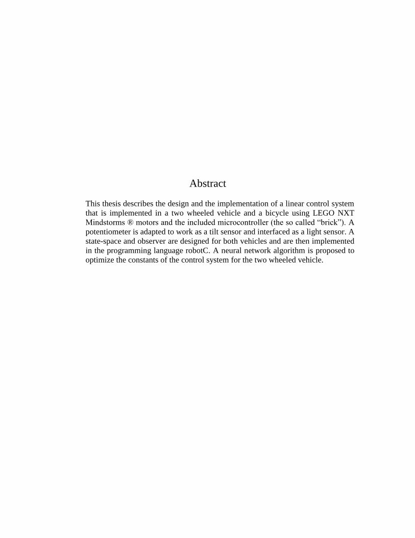
5.4.2 State-space controller design
The state space equations of bicycle are:
bahhg 1
0
0
10
01y
Were b
Vab
2
and it is assumed 0
The characteristic equation with full state-space feedback is given by:
22122 2)(det nnh
gK
h
KBKAI
For a settling time of 0.8 seconds and an overshoot of 5%:
7.0 (from graph in [11])
2.88.07.0
6.4n
Therefore: 4.221K and 0.22K
6 Future Work
In the future the observer design can be implemented in robotC in the bicycle and
different learning algorithms similar to the ones used in neural networks (not just the
Hebb rule) can also be implemented in robotC.
7 Conclusions
The PD design implemented for the two-wheeled vehicle and the bicycle gave an
acceptable first guess for the values used after trial and error. Therefore the assumptions
made for the calibration programs were sound.

References [1] David J.N. Limebeer, Robin S. Sharp, Bicycles, Motorcycles and Models. IEEE’s
Control Systems Magazine Volume 26, Issue 5.
[2] Tomas B. Co, Taylor series expansion.
http://www.chem.mtu.edu/~tbco/cm416/taylor.html
[3] K. J. Astrom, Bicycle dynamics and control.
http://audiophile.tam.cornell.edu/~als93/ohdelft.pdf
[4] Kent Lundberg, The inverted pendulum system.
http://web.mit.edu/klund/www/papers/UNP_pendulum.pdf
[5] A. L. Schwab, J. P. Meijaard, J. M. Papadopoulos, A multibody dynamics benchmark
on the equations of motion of an uncontrolled bicycle.
[6] J. P. Meijaard, Derivation of the Linearized equations for an uncontrolled bicycle.
[7] Richard C. Dorf, Robert H. Bishop, Modern Control Systems
[8] Chia-Chi Tsui, Robust Control System Design
[9] K. J. Astrom, Uncertainty and robust control,
http://www.control.lth.se/~kja/modeluncertainty.pdf
[10] Taylor series expansions for trigonometric functions,
http://www.efunda.com/math/taylor_series/trig.cfm
[11] Gene F. Franklin, J. David Powell, Abbas Emami-Naeini, Feedback Control of
Dynamic Systems.
[12] Jingang Yi, Dezhen Song, Anthony Levandowski and Suhada Jayasuriya,
Trajectory Tracking and Balance Stabilization Control of Autonomous Motorcycles
http://faculty.cs.tamu.edu/dzsong/pdfs/MotorcycleControl_ICRA06.pdf
[13] Dynamic inversion of non-linear maps with applications to non-linear control and
robotics
http://inversioninc.com/papers/thesis.pdf
[14] Fred G. Martin, Robotic Explorations: A Hands-On Introduction to Engineering
[15] Stefano Nolfi and Dario Floreano, Evolutionary Robotics: The Biology, Intelligence
and Technology of Self-Organizing Machines
[16] Yasuhito Tanaka and Toshiyuki Murakami, Self-Sustaining Bicycle Robot with
Steering Controller

[17] Faires and Burden, Numerical Methods. 2nd
edition
Appendix A: Derivation of Non-linear Equations for a Bicycle
Figure 29: Point-mass model of bicycle on left-handed coordinate system. Notice the use of an
absolute coordinate system. The intersection between the x axis and the line made by the two contact
points doesn’t have to be at the origin. Also angles and are in the z-x plane.
Fig 1 shows the point-mass model we are using. The assumptions are: all the mass
is concentrated at point m, b is the wheelbase, the wheels make point contact with the
ground and the wheels have no side slipping (nonholonomic rolling). We can follow the
derivation of equation (1) in Appendix A from Fig 2 in Appendix A:

TFhmghmh cossin2 (1)
Where TF are all the initial forces due to the bicycle turning.
Before finding those forces we can simplify the equations by omitting in the equations
by finding out more equations from the planar motion of the bicycle. The following parts
of the derivation are similar to the ones described in [1] and [13].
Figure 30: top view of the bicycle
We first start by finding out the following kinematic relations from Fig 2:

cosVx (2)
sinVy (3)
r
V (4)
tanr
b (5)
Next we find the turning angle of the bicycle in terms of the steering shaft angle .
This angle is the angle between the plane of the back wheel and the plane of the front
wheel. It is not equal to unless the inclination angle is zero as will be shown in the
following relation. The planes intersecting the back wheel, the front wheel, the ground
and a plane perpendicular to the ground make the 3D shape shown in Fig 3.

Figure 31: 3D shape resulting from the intersection of the planes intersecting the back wheel, the
front wheel, the ground and a plane perpendicular to the ground
The following relationships are derived from Fig 3:
b
ccos
a
btan
a
ctan
Combining the above relations yields:

tancostan (6)
As expected if the inclination angle is 0, .
Combining (5) and (4) with (6) yields:
cos
tan
b
V (7)
Appendix B: Demonstration of Lyapunov’s Theorem Using a Linear Control
System on a Non-linear Bicycle Model in SIMULINK
Lyapunov’s theorem states that a controller designed for a linear system at a
certain operating point will also work for the nonlinear system it was derived from on the
same operating point:

Appendix C: Derivation of rate of change of angles for the horizontal angle
sensor

Figure 32: angles and lengths of the triangle formed when the wire connected to the variable resistor
touches the ground
This derivation is used to calculate the angular position, velocity and acceleration
of 1 based on the angular position, velocity and acceleration of 3 , which is proportional
to the voltage of a variable resistor on top the board. The wire can go below the line of
the board because there is a notch in the board.
Vector sum:
321 RRR

Imaginary and real components:
Im 0sinsin 2211 RR
Re 32211 coscos RRR
213
31211 sinsin RR
The above line can also be obtained from the sin law:
1
4
2
1 sinsin
RR
31211 sinsin RR
31311
2
1 sincoscossinsinR
R (1)
1
3
321tan
sincosRR

3
3
2
1
1
1sin
cos
tanR
R
(2)
Using equation (1) and deriving with respect to time:
3111
2
1 cos aR
R (3)
Where 313131 cossinsincoscosa
aR
R
a
1
2
1
3
1
cos
(4)
Using equation (3) and deriving with respect to time:
3131
2
1111
2
1 sincos aaR
R
aR
R
aaR
R
1
2
1
331
2
11
2
1
1
cos
sin
(5)

Where 3131sin a
Equations (2), (4) and (5) can be implemented digitally either using a lookup table
or the Taylor series expansion of cosine sine and tangent functions that can be found in
[10].
Appendix D: robotC Code for Tilt Sensor Calibration Program #define INIT_ANGLE 50.0 #define ANGLE_INC 10.0 #define NUM_READINGS 8 const tSensors lightSensor = (tSensors) S1; //declaring "light sensor" in port 1 task main () { int i = 0; float degrees[NUM_READINGS]; float sensor_raw_measurements[3]; float sensor_avg_raw_measurement; float sensor_raw_value[NUM_READINGS]; float x = 0; float y = 0; float x2 = 0; float xy = 0; nNxtButtonTask = -2; //grab control of the buttons while(true) //loop {

//constants used to deal with the button interface string sTemp; TButtons nBtn;
while ((nBtn = nNxtButtonPressed) == -1) // while button is not pressed do nothing
{} if(i == NUM_READINGS){ //calculations for(i=0; i<NUM_READINGS ;i++){ x += sensor_raw_value[i]; y += degrees[i]; x2 += sensor_raw_value[i]*sensor_raw_value[i]; xy += sensor_raw_value[i]*degrees[i]; }
nxtDisplayTextLine(0, " a1 is: %.3f", (NUM_READINGS*xy - x*y) / (NUM_READINGS*x2 - x*x)); nxtDisplayTextLine(1, " a0 is: %.3f", (x2*y - xy*x) / (NUM_READINGS*x2 - x*x));
nxtDisplayTextLine(2, ""); while ((nBtn = nNxtButtonPressed) != -1) // wait for button release {}
while ((nBtn = nNxtButtonPressed) == -1) // while button is not pressed do nothing
{} break;}
nxtDisplayTextLine(0, " Angle: %.2f", degrees[i] = i*ANGLE_INC + INIT_ANGLE);
sensor_raw_measurements[0] = SensorValue(lightSensor); wait1Msec(1); sensor_raw_measurements[1] = SensorValue(lightSensor); wait1Msec(1); sensor_raw_measurements[2] = SensorValue(lightSensor); wait1Msec(1); sensor_avg_raw_measurement = (sensor_raw_measurements[0] + sensor_raw_measurements[1] + sensor_raw_measurements[2] + SensorValue(lightSensor))/4;

nxtDisplayTextLine(1, " V Measurement:"); nxtDisplayTextLine(2, " %.2f", sensor_raw_value[i] = sensor_avg_raw_measurement); i++; while ((nBtn = nNxtButtonPressed) != -1) // wait for button release {} } return; }
Appendix E: robotC Code for Motor Acceleration Calibration
Program #define NUM_ACCEL_READINGS 6 //has to be less than 10 #define NUM_ANGLE_READINGS 20 //has to be higher than 3! (check top velocity calculation) float findInitAccel(int powerLevel); task main () { int i; float initAccel; float x2 = 0; float xy = 0; //constants used to deal with the button interface string sTemp; TButtons nBtn; for(i=0; i < NUM_ACCEL_READINGS; i++){ //wait for motor to stop and then change direction (to keep the robot in one place) wait1Msec(1000); bMotorReflected[motorA] = i % 2; //get and print initial acceleration for given power level nxtDisplayTextLine(i, " %-6.2f rads/s^2", initAccel = findInitAccel(100 - 10*i));

//least squares error calculations x2 += initAccel*initAccel; xy += initAccel*(100.0 - 10.0*i); } nxtDisplayTextLine(6, ""); nxtDisplayTextLine(7, " %-6.4f pl/omg'", xy/x2); while ((nBtn = nNxtButtonPressed) != -1) // wait for button release {} while ((nBtn = nNxtButtonPressed) == -1) // while button is not pressed do nothing {} return; } float findInitAccel(int powerLevel){ int i = 0; float times[NUM_ANGLE_READINGS]; float encoder_position[NUM_ANGLE_READINGS]; float velocity[NUM_ANGLE_READINGS]; float top_velocity; float x2; float xy; //constants used to deal with the button interface string sTemp; TButtons nBtn; //synchronizing motors nSyncedMotors = synchAC; nSyncedTurnRatio = 100; //initializing motor and timers (but using only wait1Msec timer) nMotorEncoder[motorA] = 0; motor[motorA] = powerLevel; ClearTimer(T1);

for(i=0; i<NUM_ANGLE_READINGS ;i++){ //measuring time times[i] = time1[T1]; //measuring motor position encoder_position[i] = nMotorEncoder[motorA]; //differentiating using backward difference if(i == 0) velocity[i] = 0; else velocity[i] = (encoder_position[i] - encoder_position[i-1])/(times[i] - times[i-1]); //wait 20msecs for next measurement wait1Msec(20); } //stop motors motor[motorA] = 0; //calculations
top_velocity = (velocity[NUM_ANGLE_READINGS - 1] + velocity[NUM_ANGLE_READINGS - 2])/2.0;
x2 = 0; xy = 0; for(i=1; i<NUM_ANGLE_READINGS ;i++){
if(1.0 - velocity[i]/top_velocity*1.0 > 0){ //to check if numbers can be used in log function
x2 += times[i]*times[i]; xy += times[i]*-1.0*log(1.0 - velocity[i]/top_velocity); } } //Finding value return 2*PI/360*top_velocity*xy/x2*1000000.0; }
Appendix F: robotC Implementation of State-Space Controller
for Two-Wheeled Vehicle
//physical constants
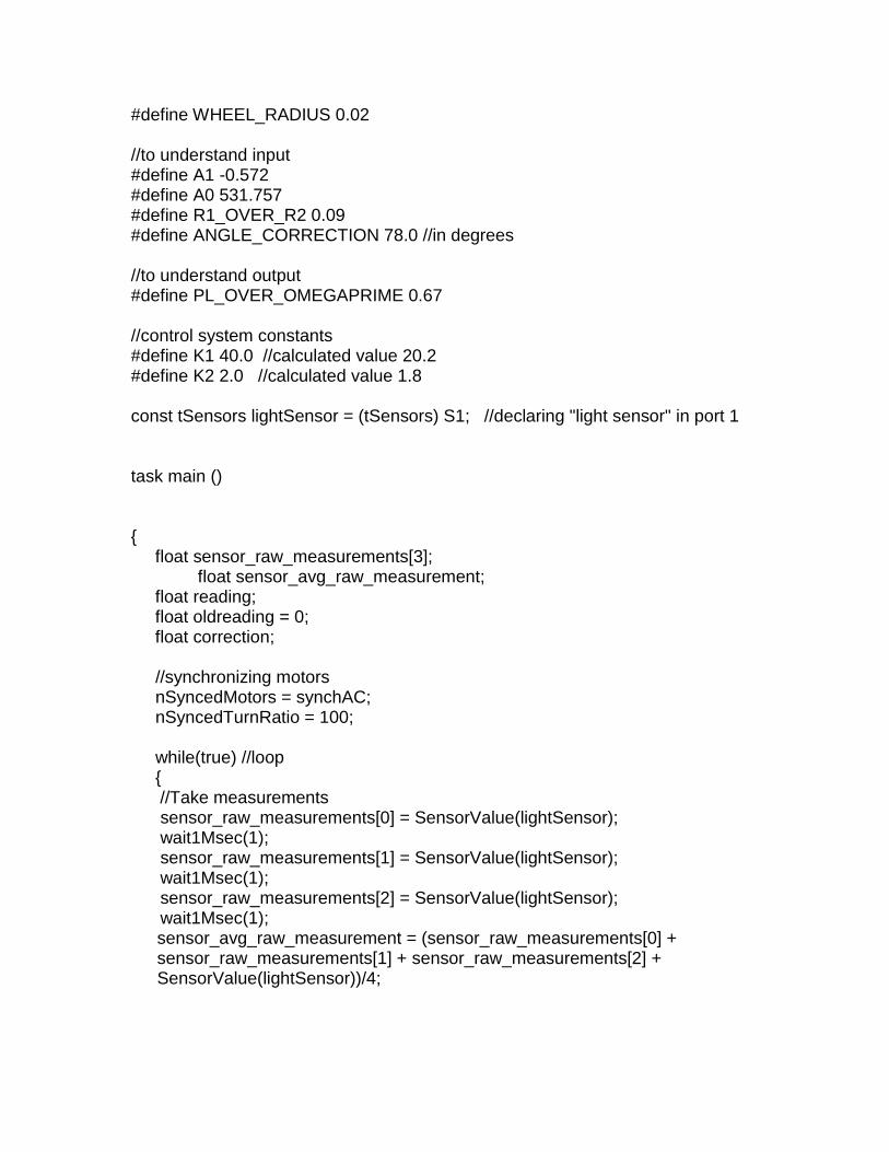
#define WHEEL_RADIUS 0.02 //to understand input #define A1 -0.572 #define A0 531.757 #define R1_OVER_R2 0.09 #define ANGLE_CORRECTION 78.0 //in degrees //to understand output #define PL_OVER_OMEGAPRIME 0.67 //control system constants #define K1 40.0 //calculated value 20.2 #define K2 2.0 //calculated value 1.8 const tSensors lightSensor = (tSensors) S1; //declaring "light sensor" in port 1 task main () { float sensor_raw_measurements[3]; float sensor_avg_raw_measurement; float reading; float oldreading = 0; float correction; //synchronizing motors nSyncedMotors = synchAC; nSyncedTurnRatio = 100; while(true) //loop { //Take measurements sensor_raw_measurements[0] = SensorValue(lightSensor); wait1Msec(1); sensor_raw_measurements[1] = SensorValue(lightSensor); wait1Msec(1); sensor_raw_measurements[2] = SensorValue(lightSensor); wait1Msec(1);
sensor_avg_raw_measurement = (sensor_raw_measurements[0] + sensor_raw_measurements[1] + sensor_raw_measurements[2] + SensorValue(lightSensor))/4;

reading = degreesToRadians(A1*sensor_avg_raw_measurement + A0 - ANGLE_CORRECTION);
correction = K1*reading + K2*(reading - oldreading)/0.01; if(correction*PL_OVER_OMEGAPRIME/WHEEL_RADIUS > 100.0) motor[motorA] = 100; if(correction*PL_OVER_OMEGAPRIME/WHEEL_RADIUS < -100.0) motor[motorA] = -100; if(correction*PL_OVER_OMEGAPRIME/WHEEL_RADIUS >= -100.0 && correction*PL_OVER_OMEGAPRIME/WHEEL_RADIUS <= 100.0)
motor[motorA] = -1.0*correction*PL_OVER_OMEGAPRIME/WHEEL_RADIUS;
oldreading = reading; //To experiment with speed of feedback wait1Msec(7); } return; }
Appendix G: robotC Implementation of State-Space Controller
for Two-Wheeled Vehicle with Observer
Appendix I: robotC Implementation of State-Space Controller for Bicycle //physical constants #define B 0.14 #define WHEEL_RADIUS 0.02 //to understand input #define A1 -0.572 #define A0 531.757 #define ANGLE_CORRECTION 87.0 //in degrees //to understand output #define PL_OVER_OMEGAPRIME 0.72 //control system constants #define K1 5.0 #define K2 -0.5

const tSensors lightSensor = (tSensors) S1; //declaring "light sensor" in port 1 task main () { float sensor_raw_measurements[3]; float sensor_avg_raw_measurement; float reading; float oldreading = 0; float backMotorPosition; float oldBackMotorPosition = 0; float correction; float velocity; //Make back motor go at max speed motor[motorA] = 100; //Wait until it reaches max speed wait1Msec(2000); while(true) //loop { //Take measurements sensor_raw_measurements[0] = SensorValue(lightSensor); wait1Msec(1); sensor_raw_measurements[1] = SensorValue(lightSensor); wait1Msec(1); sensor_raw_measurements[2] = SensorValue(lightSensor); wait1Msec(1);
sensor_avg_raw_measurement = (sensor_raw_measurements[0] + sensor_raw_measurements[1] + sensor_raw_measurements[2] + SensorValue(lightSensor))/4;
reading = degreesToRadians(A1*sensor_avg_raw_measurement + A0 - ANGLE_CORRECTION);
backMotorPosition = nMotorEncoder[motorA]; correction = K1*reading + K2*(reading - oldreading)/0.01;
velocity = degreesToRadians(backMotorPosition - oldBackMotorPosition)*WHEEL_RADIUS/0.01;
if(correction*PL_OVER_OMEGAPRIME*B/velocity/velocity/0.01/0.01 > 100.0)

motor[motorC] = 100; if(correction*PL_OVER_OMEGAPRIME*B/velocity/velocity/0.01/0.01 < - 100.0)
motor[motorC] = -100; if(correction >= -100.0 && correction <= 100.0)
motor[motorC] = correction*PL_OVER_OMEGAPRIME*B/velocity/velocity/0.01/0.01;
oldBackMotorPosition = backMotorPosition; oldreading = reading; //To experiment with speed of feedback wait1Msec(7); } return; }


![DESIGN AND IMPLEMENTATION OF LINEAR HASH STRUCTURES … · DESIGN AND IMPLEMENTATION OF LINEAR HASH STRUCTURES IN NESTED TRANSACTIONS ENVIRONMNET ... [ 15] , [ 1 6]) has a hierarchical](https://img.pdfslide.net/doc/110x75/5b9ca5b409d3f2321b8d19de/design-and-implementation-of-linear-hash-structures-design-and-implementation.jpg)