Embed Size (px)
Citation preview
Guidance Notes on Des ign and Ins ta l l a t i on o f Drag Anchors and P la te Anchors
GUIDANCE NOTES ON
DESIGN AND INSTALLATION OF DRAG ANCHORS AND PLATE ANCHORS
MARCH 2017 (Updated March 2018 – see next page)
American Bureau of Shipping Incorporated by Act of Legislature of the State of New York 1862
2017 American Bureau of Shipping. All rights reserved. ABS Plaza 16855 Northchase Drive Houston, TX 77060 USA

Updates
March 2018 consolidation includes: • March 2017 version plus Corrigenda/Editorials
F o r e w o r d
Foreword These Guidance Notes provide ABS recommendations for the design and installation of drag anchors and plate anchors for offshore service. Included in these Guidance Notes are the site investigation, methodologies for geotechnical design and structural assessment, and installation and testing recommendations for drag anchors and plate anchors. Other approaches that can be proven to produce at least an equivalent level of safety will also be considered as an alternative.
These Guidance Notes are applicable to the design of drag anchors and plate anchors, as a component of taut, semi-taut, or catenary mooring systems. These Guidance Notes are to be used with the criteria contained in the ABS Rules for Building and Classing Offshore Installations, the ABS Rules for Building and Classing Floating Production Installations, the ABS Guide for Building and Classing Floating Offshore Wind Turbine Installations, and the ABS Rules for Building and Classing Mobile Offshore Drilling Units.
These Guidance Notes become effective on the first day of the month of publication.
Users are advised to check periodically on the ABS website www.eagle.org to verify that this version of these Guidance Notes is the most current.
We welcome your feedback. Comments or suggestions can be sent electronically by email to [email protected].
Terms of Use
The information presented herein is intended solely to assist the reader in the methodologies and/or techniques discussed. These Guidance Notes do not and cannot replace the analysis and/or advice of a qualified professional. It is the responsibility of the reader to perform their own assessment and obtain professional advice. Information contained herein is considered to be pertinent at the time of publication, but may be invalidated as a result of subsequent legislations, regulations, standards, methods, and/or more updated information and the reader assumes full responsibility for compliance. This publication may not be copied or redistributed in part or in whole without prior written consent from ABS.
ABS GUIDANCE NOTES ON DESIGN AND INSTALLATION OF DRAG ANCHORS AND PLATE ANCHORS . 2017 iii
T a b l e o f C o n t e n t s
GUIDANCE NOTES ON
DESIGN AND INSTALLATION OF DRAG ANCHORS AND PLATE ANCHORS
CONTENTS SECTION 1 General .................................................................................................... 1
1 Introduction ......................................................................................... 1 3 Scope and Application ........................................................................ 1 5 Terms and Definitions ......................................................................... 1 7 Symbols and Abbreviation .................................................................. 1
7.1 Symbols ........................................................................................... 1 7.3 Abbreviations ................................................................................... 4
SECTION 2 Site Investigation .................................................................................... 5
1 General ............................................................................................... 5 3 Desk Study .......................................................................................... 5 5 Sea Floor Survey ................................................................................ 6 7 Subsurface Investigation and Testing ................................................. 6
7.1 Subsurface Investigations ................................................................ 6 7.3 Soil Testing Program ....................................................................... 7
SECTION 3 Drag Anchor ............................................................................................ 8
1 Introduction ......................................................................................... 8 3 Installation Performance ..................................................................... 8 5 Holding Capacity ................................................................................. 9
5.1 Empirical Method ........................................................................... 10 5.3 Analytical Method Based on Limit Equilibrium Principle ................ 10 5.5 Finite Element Method ................................................................... 10 5.7 Post Installation Effect ................................................................... 10 5.9 Uplift Angle .................................................................................... 10
FIGURE 1 Skematic of Drag anchor .......................................................... 8 FIGURE 2 Drag Trejectory of Drag anchor ................................................ 9
SECTION 4 Plate Anchor ......................................................................................... 11
1 Introduction ....................................................................................... 11 3 Installation Performance ................................................................... 13
3.1 General .......................................................................................... 13 3.3 VLA ................................................................................................ 14
iv ABS GUIDANCE NOTES ON DESIGN AND INSTALLATION OF DRAG ANCHORS AND PLATE ANCHORS . 2017

3.5 SEPLA ........................................................................................... 14 3.7 DEPLA........................................................................................... 15
5 Holding Capacity ............................................................................... 15 FIGURE 1 Schematic of SEPLA ............................................................... 11 FIGURE 2 Installation Process for Suction Embedded Plate Anchor ...... 12 FIGURE 3 Installation Process of DEPLA ................................................ 13
SECTION 5 Commentary on Structural Assessment ............................................ 17
1 General ............................................................................................. 17 3 Yielding Check .................................................................................. 17 5 Fatigue Assessment ......................................................................... 17 7 Anchor Reverse Catenary Line ......................................................... 17 9 Buckling Assessment ........................................................................ 17
SECTION 6 Anchor Installation ............................................................................... 18
1 General ............................................................................................. 18 3 Installation Monitoring ....................................................................... 18
APPENDIX 1 Analytical Method for Drag Anchor Design and Design Procedure
Recommendation ................................................................................. 19 1 General ............................................................................................. 19 3 Analytical Model ................................................................................ 19
3.1 Anchor Holding Capacity Under Combined Load .......................... 19 3.3 Kinematic Behavior ....................................................................... 21 3.5 Embedded Anchor Line Equilibrium Equation ............................... 22
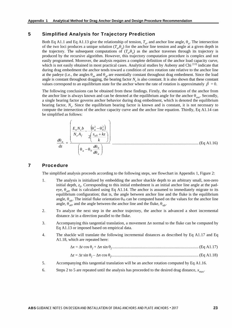
5 Simplified Analysis for Trajectory Prediction ..................................... 23 7 Procedure ......................................................................................... 23 9 Recommended Design Procedure .................................................... 24 11 Work Example ................................................................................... 25
11.1 Design Parameters ........................................................................ 25 11.3 Predicted Anchor Trajectory and Holding Capacity ....................... 26 11.5 Anchor Design ............................................................................... 26
TABLE 1 Values of Interaction Coefficient ............................................. 21 TABLE 2 Design Parameter for Drag Anchor Trajectory Prediction ...... 26 FIGURE 1 Drag Anchor Definition ............................................................ 20 FIGURE 2 Flowchart for Drag Anchor Trajectory Prediction .................... 24 FIGURE 3 Design Procedure for Drag Anchor Trajectory Prediction....... 25 FIGURE 4 Anchor Trajectory Prediction during Drag Embedment .......... 27 FIGURE 5 Anchor Tension during Drag Embedment .............................. 27 FIGURE 6 Fluke Angle during Drag Embedment ..................................... 27
ABS GUIDANCE NOTES ON DESIGN AND INSTALLATION OF DRAG ANCHORS AND PLATE ANCHORS . 2017 v
APPENDIX 2 Cyclic Loading Effect ........................................................................... 28 1 General ............................................................................................. 28 3 Cyclic Shear Strength ....................................................................... 28 5 Procedure .......................................................................................... 29
5.1 Design Storm Composition and Cycle Counting ............................ 29 5.3 Equivalent Number of Cycles to Failure ......................................... 30 5.5 Cyclic Contour Diagram ................................................................. 30 5.7 Description of Procedure ............................................................... 30
FIGURE 1 Typical Cyclic Shear Stress .................................................... 28 FIGURE 2 Example of Transformation of Cyclic Loading History to
Constant Cyclic Parcels .......................................................... 30 APPENDIX 3 Set-up Effect ......................................................................................... 32 APPENDIX 4 Capacity Factor for Plate Anchors in Cohesive Soil ......................... 33
1 Capacity Factor in Soil with Constant Shear Strength with Depth .... 33 3 Capacity Factor in Soil with Linearly Increasing Shear Strength ...... 34 5 Capacity Factor in Layered Soil ........................................................ 34 FIGURE 1 Capacity Factor for Soil with Constant Shear Strength .......... 33 FIGURE 2 Capacity Factor for Soil with Linearly Increasing Shear
Strength ................................................................................... 34 APPENDIX 5 Loss of Embedment During Keying for SEPLA ................................. 35 APPENDIX 6 Methodology to Calculate the Anchor Reverse Catenary Line......... 36
1 General ............................................................................................. 36 3 Equilibrium Equations of Embedded Anchor Line ............................ 37 5 Simplified Solution for the Mooring Catenary Line............................ 38 7 Description of Procedure .................................................................. 40 9 Work Example ................................................................................... 41 TABLE 1 Effective Surface and Bearing Area for Anchor Line .............. 38 TABLE 2 Parameters for the Work Example .......................................... 41 FIGURE 1 General Arrangement of Anchor Line for Plate Anchor .......... 36 FIGURE 2 Force Equilibrium of Anchor Line Element ............................. 37 FIGURE 3 Soil Strength Adjustment to Account for Anchor Line
Weight ..................................................................................... 40 FIGURE 4 Anchor Line Profile for the Work Example .............................. 41
vi ABS GUIDANCE NOTES ON DESIGN AND INSTALLATION OF DRAG ANCHORS AND PLATE ANCHORS . 2017

APPENDIX 7 Commentary on Acceptance Criteria ................................................. 42 1 General ............................................................................................. 42 3 Factor of Safety for Drag anchor ...................................................... 42 5 Factor of Safety for Plate Anchor ...................................................... 43 7 Acceptance Criteria for Yielding ....................................................... 44 9 Acceptance Criteria for Fatigue ........................................................ 44 TABLE 1 Factor of Safety for Drag anchor Holding Capacities ............. 42 TABLE 2 The Coefficient of Friction for Mooring Line ............................ 43 TABLE 3 Factor of Safety for Plate Anchor ............................................ 43
APPENDIX 8 References ............................................................................................ 45
ABS GUIDANCE NOTES ON DESIGN AND INSTALLATION OF DRAG ANCHORS AND PLATE ANCHORS . 2017 vii

This Page Intentionally Left Blank
S e c t i o n 1 : I n t r o d u c t i o n
S E C T I O N 1 General
1 Introduction The purpose of these Guidance Notes is to provide recommendations for the design and installation of drag anchors and plate anchors for taut, semi-taut or catenary mooring systems. These Guidance Notes are to be used in conjunction with the ABS Rules for Building and Classing Offshore Installations (OI Rules), the ABS Rules for Building and Classing Floating Production Installations (FPI Rules), the ABS Guide for Building and Classing Floating Offshore Wind Turbine Installations (FOWTI Guide), and the ABS Rules for Building and Classing Mobile Offshore Drilling Units (MODU Rules).
3 Scope and Application These Guidance Notes cover the geotechnical design, structural assessment and installation for both drag anchors and plate anchors.
5 Terms and Definitions DIP follower: The dynamically installed pile (DIP) used to install the dynamically embedded plate anchor (DEPLA) by self-weight penetration.
Embedment ratio: The ratio of anchor embedment depth to the width of anchor fluke.
Keying: The process that a plate anchor is pulled and rotated until the plate surface is perpendicular to the load direction to achieve the maximum capacity.
Loss of embedment: Vertical displacement at the center of the anchor fluke during keying.
Soil overburden pressure: The pressure caused by the soil self-weight. It is defined as the soil unit weight times the anchor embedment depth.
Soil non-homogeneity: A non-dimensional factor to represent the non-homogeneity of the soil. It is defined as the rate of increasing undrained shear strength with depth time the width of the anchor fluke divided by the soil undrained shear strength (kB/su).
Suction follower: The suction caisson that used to penetrate the plate anchor and can be reused to install the suction embedded plate anchor.
Thickness ratio: The ratio of plate anchor fluke width to thickness.
7 Symbols and Abbreviation
7.1 Symbols Af = area of the anchor fluke
Aplate = projected maximum fluke area perpendicular to the direction of pullout
Ain = plan view of inside area where suction pressure is applied
Ainside = inside lateral area of the suction follower
Awall = sum of inside and outside wall area embedded into soil
Atip = vertical projected sectional area for both suction follower and plate anchor
ABS GUIDANCE NOTES ON DESIGN AND INSTALLATION OF DRAG ANCHORS AND PLATE ANCHORS . 2017 1

Section 1 General
B = width of the plate
b = chain bar or wire diameter
d = nominal diameter of chain, or diameter of wire or rope.
D = outside diameter of the suction follower
Dwater = water depth
e = loading eccentricity
ef = loading eccentricity for friction resistance
ew = loading eccentricity for anchor weight
Et = multipliers to give the effective widths in the tangential direction
En = multipliers to give the effective widths in the normal direction
F = resistance offered by the soil tangential to the chain (per unit length)
Ffriction = friction of mooring line on the sea bed
fs = anchor shank resistance
fsl = frictional coefficient of mooring line on sea bed at sliding
Fanchor = maximum load at anchor for design environmental condition
FOS = factor of safety
k = rate of increasing of undrained shear strength with depth
L = length of the plate
Lbed = length of mooring line on seabed at the design storm condition
M0 = initial moment corresponding to zero net vertical load on the anchor
Nc = bearing capacity factor
Ne = bearing capacity factor under combined loading
Nq = bearing capacity factor, depending on the friction angle
Nn,max = bearing capacity factor under condition of pure normal loading
Nt,max = bearing capacity factor under condition of pure tangential loading
Nm,max = bearing capacity factor under condition of pure moment loading
Pline = maximum mooring line tension
Q = resistance offered by the soil normal to the chain (per unit length)
Qave = average bearing resistance per unit length of chain over the soil depth D
Q1 = normalized soil resistance due to mudline strength
Q2 = normalized soil resistance due to strength gradient
Qtot = total penetration resistance
Ranchor = holding capacity of drag anchor
RPLA = holding capacity of plate anchor
s = distance measured along the chain
2 ABS GUIDANCE NOTES ON DESIGN AND INSTALLATION OF DRAG ANCHORS AND PLATE ANCHORS . 2017
Section 1 General
su = undrained shear strength of soil at the depth of anchor fluke
AVEtipus = average of triaxial compression, triaxial extension, and direct simple shear (DSS) undrained
shear strength at anchor tip level,
DSSus = direct simple shear strength
su,r = remolded undrained shear strength
su0 = undrain shear strength at mudline
St = soil sensitivity
t = thickness of the anchor fluke
T = tension of the chain
Ta = tension at the attachment point
T0 = tension at the mudline
T* = normalized tension
µ = coefficient
w = anchor line self-weight per unit length
Wsub = submerged unit weight of mooring line
W′ = submerged weight during installation
aW ′ = difference between the anchor weight in air and the anchor buoyancy force in soil
x = horizontal length of the mooring line from anchor
x* = x/D
∆z = loss of anchor embedment
z = anchor embedment depth
z′ = embedment depth of the mooring line from the mudline
z* = z′/D
ztip = tip penetration depth
αins = adhesion factor during installation, it is usually defined as the ratio of remolded shear strength over undisturbed shear strength
α = adhesion factor for anchor line
γ′ = effective unit weight of soil
γ = soil unit weight
η = reduction for soil disturbance due to penetration and keying
σeqv = equivalent Von Mises stress
σyield = yield stress of the considered anchor structural component
β = load inclination during the keying
τa = average shear stress
τcy = cyclic shear stress amplitude
ABS GUIDANCE NOTES ON DESIGN AND INSTALLATION OF DRAG ANCHORS AND PLATE ANCHORS . 2017 3
Section 1 General
τf,cy = cyclic shear strength
τ0 = initial soil shear stress prior to the installation of anchor
θ = orientation of the chain to the horizontal
θa = anchor line angle from horizontal at shackle point
θf = fluke angle to horizontal
θ0 = angle of anchor line from horizontal at mudline
δ = interface friction angle at soil-mooring line interface
7.3 Abbreviations CPTU piezocone penetrometer test
DEC Design Environmental Condition
DEPLA dynamically embedded plate anchor
DIP dynamically installed pile
DSS direct simple shear
SEPLA suction embedded plate anchor
VLA vertical loaded anchor
4 ABS GUIDANCE NOTES ON DESIGN AND INSTALLATION OF DRAG ANCHORS AND PLATE ANCHORS . 2017

S e c t i o n 2 : S i t e I n v e s t i g a t i o n
S E C T I O N 2 Site Investigation
1 General Site investigation is conducted to determine the seabed stratigraphy and soil engineering parameters for the anchor design and geohazards analysis. Generally, the procedure for the site investigation program should include:
• Desk study to obtain regional and relevant data for the site
• Sea floor survey to obtain relevant geophysical data
• Subsurface investigation and test to obtain the necessary geotechnical data
• Additional sea floor survey and/or subsurface investigation and/or laboratory test as required
Depending on the size of a project and/or the complexity of the geotechnical context and associated risks (geohazards), additional intermediate stages may be necessary.
The site investigation should satisfy the requirements given in 3-2-5/3 of the OI Rules.
It is important that the geophysical and geotechnical components are planned together as integrated parts of the same investigation. Data analyses should be considered as a single exercise drawing together with the results of geological, geophysical, hydrographic and geotechnical work, performed by specialists, in an integrated manner into one final report.
3 Desk Study The desk study assembles existing data for the preliminary site assessment and will formulate requirements for subsequent sea floor surveys and subsurface investigations. The desk study should include a review of all sources of appropriate information, collect and evaluate all available relevant data for the site including:
• Bathymetric information
• Regional geological data
• Regional meteorological and oceanographic data
• Information and records of seismic activity
• Existing geotechnical data and information
• Previous experience with foundations in the area
Data of the regional geological characteristics is also to be used to verify that the findings of the subsurface investigation are consistent with known geological conditions. An assessment of the seismic activity, fault plane, seafloor instability, scour and sediment mobility, shallow gas and seabed subsidence are used when necessary.
ABS GUIDANCE NOTES ON DESIGN AND INSTALLATION OF DRAG ANCHORS AND PLATE ANCHORS . 2017 5
Section 2 Site Investigation
5 Sea Floor Survey Geophysical data for the conditions existing at and near the surface of the sea floor should be obtained during the sea floor survey. It should provide information about the soil stratigraphy, local soil condition and evidence of geological features. The geophysical survey report should be provided for the scope of the geotechnical investigation. It should be performed before geotechnical investigation. Geophysical survey should provide qualitative assessment across site. So whenever possible, the acquired geophysical data should be used in the subsequent planning of the geotechnical site investigation which provides quantitative assessment. The following information should be obtained where applicable:
• Seafloor bathymetry and topography (particularly in area of uneven seafloor, outcrops, corals, pockmarks, sand waves, etc.) – by echo-sounding or swath echo-sounding
• Seafloor features and obstructions (e.g., the presence of boulders, small craters, faults, scarps and run outs from debris flows) – by side-scan sonar
• Seabed sub-bottom profiling to define structural features within the near surface sediments –by means of reflection seismic systems or seismic refraction systems
The kinds and sizes of features that can be identified with these surveys depend on the resolution of the data. Different survey types with their uses, features that can be identified, typical resolution limits and advantages and limitations can be referred to ABS Guidance Notes on Subsea Pipeline Route Determination. It is recommended that a high-quality, high-resolution geophysical survey be performed. The minimum survey area for the geophysical survey should be the full extent of anchor spread. For drag anchors, the extension of site investigation may increase due to the associated large drag distance. The regional geophysical survey is a convenient starting point since it is collected to support oil and gas exploration over the reservoir or field development area and is typically available early in the process.
The seabed location of the anchors may change due to changes in mooring lines lengths and/or headings, field layout, platform properties, and mooring leg properties during the detailed platform and mooring design process. This should be taken into consideration in the site investigation program.
The following information should be obtained where applicable to the planned anchor design.
• Soundings or contours of the sea bed
• Presence of boulders, obstructions, and small craters
• Gas seeps
• Shallow faults
• Slump blocks
• Subsea permafrost or ice bonded soils
7 Subsurface Investigation and Testing The subsurface investigation and testing program is to obtain reliable geotechnical data concerning the stratigraphy and properties of the soil. This data is to be used to assess whether the desired level of structural safety and performance can be obtained and the feasibility of the proposed method of installation.
7.1 Subsurface Investigations As the quality of soil sample is expected to decrease with increasing water depth, the use of in-situ testing techniques is encouraged for deepwater sites. Typical tools used include remote vane, piezoprobe, CPTU (piezocone penetrometer tests), T-bar or ball penetrometer, etc. The required depth of site investigation is at least the anticipated design penetration depth plus a consideration for the zone of influence of the loads imposed by the base of the foundation. The zone of influence should be at least the anchor diameter or anchor fluke width [1]. The sampling frequency and depth of sampling will depend on a number of project-specific factors such as the number of anchor locations, soil stratigraphy and water depth. Typically, soil characterization is performed at each anchor location or at each anchor group for a group mooring pattern,
6 ABS GUIDANCE NOTES ON DESIGN AND INSTALLATION OF DRAG ANCHORS AND PLATE ANCHORS . 2017
Section 2 Site Investigation
or at least at two locations per anchor cluster over the anchor pattern if the interpretation of the survey shows little variation in soil properties across the pattern. However, if high-quality geotechnical data already exists in the general vicinity of the anchor pattern then little variation of soil properties is inferred over the areal extent of the foundation. However if extensive experience with the chosen foundation concept in the area can be drawn upon, the above recommendations may be modified as appropriate. For anchors such as drag anchors, the extension of site investigation may increase due to the associated large drag distance. If the soil investigation is performed primarily using CPTU, it is recommended that at least one boring with sampling be taken to properly calibrate the CPTU results. This boring/core should be taken at one of the CPTU locations.
7.3 Soil Testing Program The soil testing program is to reveal the necessary engineering properties of the soil including strength, classification and deformation properties of the soil. Testing should be performed in accordance with recognized standards, such as ASTM standards.
The soil testing program is to be in accordance with the OI Rules.
For the anchoring system, additional tests should be considered to adequately describe the creep and set-up characteristics of the soil as well as the cyclic soil shear strength properties for the reliable design.
If the reference site is within a seismic zone, geotechnical investigations should include tests to determine dynamic soil properties and liquefaction potential.
ABS GUIDANCE NOTES ON DESIGN AND INSTALLATION OF DRAG ANCHORS AND PLATE ANCHORS . 2017 7
S e c t i o n 3 : D r a g A n c h o r
S E C T I O N 3 Drag Anchor
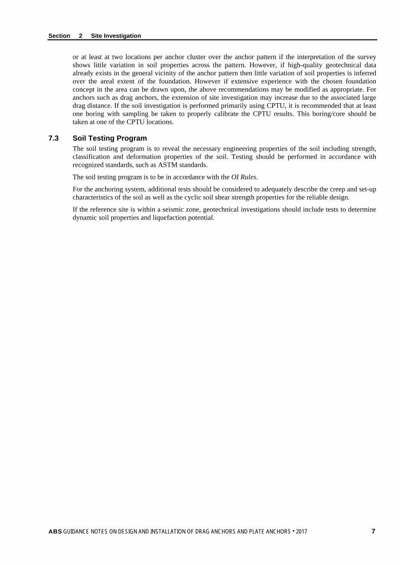
1 Introduction The drag anchor is designed to penetrate into the seabed, either partly or fully. The holding capacity of the drag anchor is generated by the resistance of the soil in front of the anchor. The drag anchor is more suitable for resisting large horizontal loads.
FIGURE 1 Skematic of Drag anchor
The main components of a drag anchor are fluke, shank, shackle and chain or wire, shown in Section 3, Figure 1. The fluke-shank angle (θfs) is normally between 30° and 50°, with the lower angle used for sand or stiff clay and the higher one for soft clay. A fluke-shank angle in between these is more appropriate in certain layered soil conditions. When an anchor is used in very soft clay (mud) with the fluke-shank angle set at 30°, the anchor penetration depth will be less than the case when the fluke-shank angle is 50°, consequently the holding capacity will be lower. It is also found that the anchor penetrates deeper when the anchor is connected to wire rope compared to that connected to chain. Hence, the anchor connected to wire rope will yield higher holding capacity.
3 Installation Performance Drag embedded anchors are installed by dragging the anchor through the soil. The applying load is generally equal to the maximum design load determined by dynamic analyses for the intact design condition. After installation the anchor is capable of resisting loads equal to the installation load without further penetration.
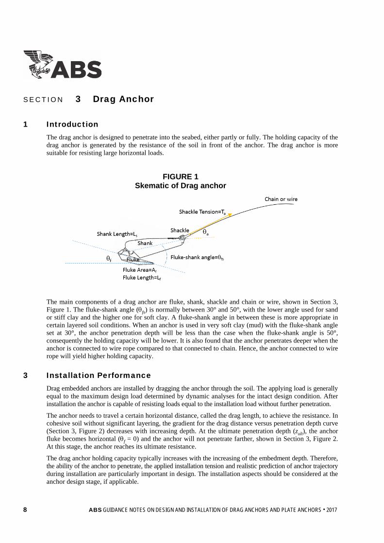
The anchor needs to travel a certain horizontal distance, called the drag length, to achieve the resistance. In cohesive soil without significant layering, the gradient for the drag distance versus penetration depth curve (Section 3, Figure 2) decreases with increasing depth. At the ultimate penetration depth (zult), the anchor fluke becomes horizontal (θf = 0) and the anchor will not penetrate farther, shown in Section 3, Figure 2. At this stage, the anchor reaches its ultimate resistance.
The drag anchor holding capacity typically increases with the increasing of the embedment depth. Therefore, the ability of the anchor to penetrate, the applied installation tension and realistic prediction of anchor trajectory during installation are particularly important in design. The installation aspects should be considered at the anchor design stage, if applicable.
8 ABS GUIDANCE NOTES ON DESIGN AND INSTALLATION OF DRAG ANCHORS AND PLATE ANCHORS . 2017
Section 3 Drag Anchor
The geotechnical design of drag anchor should include the following if applicable:
• Anchor resistance and anchor trajectory during installation
• Anchor ultimate holding capacity
• Post installation effects (i.e., setup effects and cyclic loading effects)
• Additional drag under damaged case with one mooring line broken conditions, if applicable
• Maximum allowable additional drag
The recommended design procedure for drag anchor in soft to medium stiff clay is presented in Appendix 1. This procedure is based on the limit equilibrium method, see Appendix 1 for more details. The tension force along the anchor mooring line as well as the shape of the anchor line are illustrated in Appendix 6.
FIGURE 2 Drag Trejectory of Drag anchor
5 Holding Capacity The holding capacity of a drag embedded anchor depends on the anchor type, opening angle of the flukes, anchor size, embedded depth, stability of the anchor during dragging, soil strength characteristics, type and size of chain or rope, and installation procedure, etc. The opening angle of the fluke for drag embedded anchor used in clay is usually larger than that used in sand.
The methods to determine the drag embedded anchor holding capacity can be classified as the following:
• Empirical method
• Analytical method based on limit equilibrium principles
• Finite element method
In order to yield reliable predictions, all these methods need to be calibrated against lab or field test.
ABS GUIDANCE NOTES ON DESIGN AND INSTALLATION OF DRAG ANCHORS AND PLATE ANCHORS . 2017 9
Section 3 Drag Anchor
5.1 Empirical Method The empirical method for determination of the anchor holding capacity is using a power formulae in which the ultimate anchor resistance (when the anchor penetration depth reaches the ultimate depth, zult) is related to the anchor weight. Naval Facilities Engineering Service Center (NAVFAC) [2] published design curves which represent in general the lower bounds of the test data and are suitable for “soft clay” and “sand”. These design curves have been adopted in API RP 2SK [1] and ISO 19901-7 [3]. However, the design curves suffer from the limitations in the database and inaccuracies due to scale effect using extrapolation from small size anchor tests to prototype anchors.
5.3 Analytical Method Based on Limit Equilibrium Principle The analytical method satisfies the equilibrium equations for both the drag anchor and the embedded anchor line. It takes into account a more detailed site specific soil condition and different anchor geometry. It could provide detailed anchor performance information during installation such as the anchor trajectory, anchor rotation, anchor ultimate holding capacity and the relationship between line tension and anchor penetration.
Analytical methods to obtain the anchor holding capacity based on the limit equilibrium principle for soft to medium stiff clay are illustrated in Appendix 1. In other soils like stiff clay, dense sand, layered soil, cemented carbonate sand, and coral, etc., the analytical method is not yet mature. The methodology to calculate the anchor reverse catenary line is illustrated in Appendix 6.
5.5 Finite Element Method The finite element method can obtain a rigorous solution for all aspects of anchor design. It is able to find the critical failure mechanism without prior assumptions and can assess complex anchor geometries, spatially varying soil properties and nonlinear material behaviors. The major limitation of the finite element method is the large time and effort required to formulate, set up and solve, even for a simple anchor trajectory.
5.7 Post Installation Effect The post installation effects (i.e., cyclic loading effect and setup effect) on the anchor holding capacity may be considered if applicable.
Cyclic loading tends to affect the soil’s undrained shear strength in two ways. First, cyclic loadings generally tend to break down the soil structure and degrade the strength. Secondly, there can be an increase in the soil’s undrained shear strength due to the high loading rate from wave frequency load cycles compared with the monotonic load. The first effect is most pronounced when the soil is subjected to a two-way cyclic loading (with load reversals) and increases with increasing over consolidation ratio of the soil. Since the mooring line is always in tension (no load reversals), there is less degradation effect on the shear strength. The net effect of cyclic loading is mostly the increase of the soil’s undrained shear strength. See Appendix 2 for more details.
The set-up effect is caused by clay thixotropy as well as clay consolidation after the anchor installation. Following disturbance and remolding during installation, the soil shear strength in the vicinity of the anchor can gradually increase with time due to the set-up effect. See Appendix 3 for more details.
It is a conservative approach to disregard the effects of cyclic loading and set-up in design. If the increase in the anchor resistance due to these two effects is taken into account in soft/medium stiff clays, the detailed analysis based on laboratory tests should be verified.
5.9 Uplift Angle According to the FPI Rules, the design of drag anchors is typically based on the requirement of zero uplift angle at the seabed for both installation and operation.
The design criteria for holding capacity of drag anchor is to be assessed for both intact condition and broken line condition, see Appendix 7 for details.
Field tests are necessary and the requirement can be found in Section 6-1-3 of the FPI Rules.
10 ABS GUIDANCE NOTES ON DESIGN AND INSTALLATION OF DRAG ANCHORS AND PLATE ANCHORS . 2017
S e c t i o n 4 : P l a t e A n c h o r
S E C T I O N 4 Plate Anchor
1 Introduction Plate anchors can be divided into two categories: drag-in plate anchor and push-in plate anchor. The drag-in plate anchor is installed by dragging the anchor through the soil in a manner similar to conventional drag anchor. This is described in Section 3. Vertical loaded anchors (VLA) are one of the most common drag-in plate anchors. The push-in plate anchor can be installed by gravity, hydraulic, propellant, impact hammer or suction. The suction embedded plate anchor (SEPLA), dynamically embedded plate anchor (DEPLA), impact/vibratory driven anchor and jetted-in anchor [1] are types of push-in plate anchor. Plate anchors have significant advantages due to their high ratio of holding capacity to weight and high vertical capacity. Once the plate anchor has reached the required penetration depth, the anchor will be rotated to the position perpendicular to the loading direction to achieve the maximum resistance. Hence, the plate anchor is mostly used in cohesive soil. This section focuses on the design and installation of plate anchors in cohesive soil.
According to Vryhof (2015) [4], the main components of a drag-in plate anchor are the shank, the fluke and the shackle. The major difference of the drag-in plate anchor from drag anchor is that the anchor will be triggered to create normal loading against the fluke when the target installation load has been reached. The anchor can withstand both horizontal and vertical loads when the anchor mode is changed from the installation mode to the vertical loading mode. During installation, the anchor is first placed on the seafloor. It will penetrate into the soil as the anchor is pulled along the bottom. Initially, the anchor dives more or less parallel to the fluke, eventually rotating such that the installation line tension is achieved. Then the anchor is pulled until the anchor fluke becomes perpendicular to the anchor line.
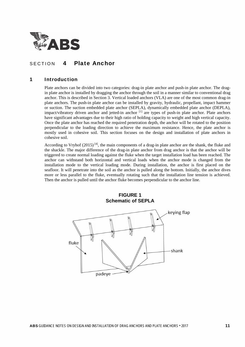
FIGURE 1 Schematic of SEPLA
ABS GUIDANCE NOTES ON DESIGN AND INSTALLATION OF DRAG ANCHORS AND PLATE ANCHORS . 2017 11
Section 4 Plate Anchor
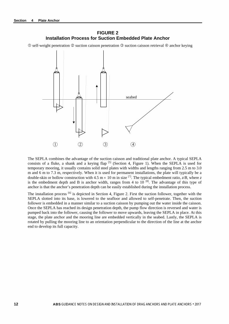
FIGURE 2 Installation Process for Suction Embedded Plate Anchor
self-weight penetration suction caisson penetration suction caisson retrieval anchor keying
seabed
21 3 4
The SEPLA combines the advantage of the suction caisson and traditional plate anchor. A typical SEPLA consists of a fluke, a shank and a keying flap [5] (Section 4, Figure 1). When the SEPLA is used for temporary mooring, it usually contains solid steel plates with widths and lengths ranging from 2.5 m to 3.0 m and 6 m to 7.3 m, respectively. When it is used for permanent installations, the plate will typically be a double-skin or hollow construction with 4.5 m × 10 m in size [7]. The typical embedment ratio, z/B, where z is the embedment depth and B is anchor width, ranges from 4 to 10 [8]. The advantage of this type of anchor is that the anchor’s penetration depth can be easily established during the installation process.
The installation process [6] is depicted in Section 4, Figure 2. First the suction follower, together with the SEPLA slotted into its base, is lowered to the seafloor and allowed to self-penetrate. Then, the suction follower is embedded in a manner similar to a suction caisson by pumping out the water inside the caisson. Once the SEPLA has reached its design penetration depth, the pump flow direction is reversed and water is pumped back into the follower, causing the follower to move upwards, leaving the SEPLA in place. At this stage, the plate anchor and the mooring line are embedded vertically in the seabed. Lastly, the SEPLA is rotated by pulling the mooring line to an orientation perpendicular to the direction of the line at the anchor end to develop its full capacity.
12 ABS GUIDANCE NOTES ON DESIGN AND INSTALLATION OF DRAG ANCHORS AND PLATE ANCHORS . 2017
Section 4 Plate Anchor
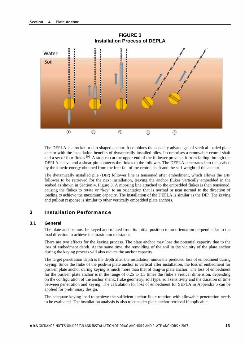
FIGURE 3 Installation Process of DEPLA
The DEPLA is a rocket or dart shaped anchor. It combines the capacity advantages of vertical loaded plate anchor with the installation benefits of dynamically installed piles. It comprises a removable central shaft and a set of four flukes [9]. A stop cap at the upper end of the follower prevents it from falling through the DEPLA sleeve and a shear pin connects the flukes to the follower. The DEPLA penetrates into the seabed by the kinetic energy obtained from the free-fall of the central shaft and the self-weight of the anchor.
The dynamically installed pile (DIP) follower line is tensioned after embedment, which allows the DIP follower to be retrieved for the next installation, leaving the anchor flukes vertically embedded in the seabed as shown in Section 4, Figure 3. A mooring line attached to the embedded flukes is then tensioned, causing the flukes to rotate or “key” to an orientation that is normal or near normal to the direction of loading to achieve the maximum capacity. The installation of the DEPLA is similar as the DIP. The keying and pullout response is similar to other vertically embedded plate anchors.
3 Installation Performance
3.1 General The plate anchor must be keyed and rotated from its initial position to an orientation perpendicular to the load direction to achieve the maximum resistance.
There are two effects for the keying process. The plate anchor may lose the potential capacity due to the loss of embedment depth. At the same time, the remolding of the soil in the vicinity of the plate anchor during the keying process will also reduce the anchor capacity.
The target penetration depth is the depth after the installation minus the predicted loss of embedment during keying. Since the fluke of the push-in plate anchor is vertical after installation, the loss of embedment for push-in plate anchor during keying is much more than that of drag-in plate anchor. The loss of embedment for the push-in plate anchor is in the range of 0.25 to 1.5 times the fluke’s vertical dimension, depending on the configuration of the anchor shank, fluke geometry, soil type, soil sensitivity and the duration of time between penetration and keying. The calculation for loss of embedment for SEPLA in Appendix 5 can be applied for preliminary design.
The adequate keying load to achieve the sufficient anchor fluke rotation with allowable penetration needs to be evaluated. The installation analysis is also to consider plate anchor retrieval if applicable.
ABS GUIDANCE NOTES ON DESIGN AND INSTALLATION OF DRAG ANCHORS AND PLATE ANCHORS . 2017 13

Section 4 Plate Anchor
3.3 VLA The capacity of a drag-in plate anchor depends on its final orientation and depth below the seabed. The prediction of the anchor trajectory during installation is a critical issue. The prediction of the drag-in plate anchor trajectory is similar as the drag anchor as illustrated in Appendix 1.
During installation, the load arrives at an angle of approximately 45° to 60° to the fluke. The load is always perpendicular to the fluke after triggering the anchor to the normal load position. This change in load direction generates 2.5 to 3 times more holding capacity in relation to the installation load.
3.5 SEPLA The risk of causing uplift of the soil plug inside the suction follower should also be considered. The suction pressure to embed the suction follower should be between the required suction pressure and allowable pressure.
Installation analysis of the suction follower is necessary to be verified. In this case the SEPLA can be penetrated to the design penetration depth and the suction follower can be retrieved for the next installation. The risk of causing uplift of the soil plug inside the suction follower should also be considered. The suction pressure to embed the suction follower should be between the required suction pressure and allowable pressure.
• The required suction pressure to embed the suction follower can be calculated as follows:
∆Ureq = in
tot
AWQ ′−
.................................................................................................................. (Eq 4.1)
• The required suction pressure to retrieve the suction follower can be calculated as follows:
(Ureq)retr = in
tot
AWQ ′+ ............................................................................................................. (Eq 4.2)
• The allowable suction pressure is defined as the maximum pressure that can be applied to the suction caisson. It is calculated as the critical pressure divided by a factor of safety. The factor of safety is typically a minimum of 1.5. The critical suction pressure can be calculated as follows:
∆Ucrit = ( )
in
AVEuinsinsideuc A
sAsN DSS
AVEtip
⋅⋅+⋅
α ......................................................................... (Eq 4.3)
where
Qtot = total penetration resistance
W′ = submerged weight during installation
Ain = plan view inside area where suction pressure is applied
Nc = bearing capacity factor, values of Nc different than the values from the following equation [10] are acceptable provided that they can be documented by appropriate modeling and test results
=
×+
Dztip201 . × 6 for
Dztip < 2.5
= 9 for D
ztip ≥ 2.5
AVEtipus = average of triaxial compression, triaxial extension, and direct simple shear (DSS)
undrained shear strength at anchor tip level
Ainside = inside lateral area of the suction follower
14 ABS GUIDANCE NOTES ON DESIGN AND INSTALLATION OF DRAG ANCHORS AND PLATE ANCHORS . 2017

Section 4 Plate Anchor
αins = adhesion factor during installation, it is usually defined as the ratio of remolded shear strength over undisturbed shear strength
DSSus = DSS undrained shear strength
D = outside diameter of the suction follower
ztip = tip penetration depth
The total penetration resistance can be calculated as the sum of the side shear and end bearing as follows:
Qtot = Awall ⋅ ( )AVEuins DSS
s⋅α + tipuc AzsN AVEtip
⋅
⋅γ′+⋅ ......................................................... (Eq 4.4)
where
Awall = sum of inside and outside wall area embedded into soil
γ′ = effective unit weight of soil
Atip = vertical projected sectional area for both suction follower and plate anchor
3.7 DEPLA Since the penetration of the DEPLA is the same as the DIP, the prediction of the penetration depth can refer to the ABS Guidance Notes on Design and Installation of Dynamically Installed Piles.
The required force to retrieve the anchor central shaft might be calculated based on the pile capacity from ABS Guidance Notes on Design and Installation of Dynamically Installed Piles. It should be noted that the retrieve force might be higher than the DIP short-term holding capacity due to soil set-up. The maximum extraction load on the steel structure of the padeye of the central shaft also should be considered.
5 Holding Capacity The plate anchor can take very high vertical load. The ultimate holding capacity of plate anchors is often defined as the ultimate pull-out capacity. It is a function of the soil undrained shear strength at the anchor fluke, the projected area of the fluke, the fluke shape and the bearing capacity factor.
The ultimate holding capacity of a plate anchor can be calculated by the following equation:
RPLA = ηsuNcAplate
+LB370630 .. ........................................................................................ (Eq 4.5)
where
η = reduction for soil disturbance due to penetration and keying. The value should be based on reliable test data. It is assumed as 0.75 if no test data provided.
su = undrained shear strength of soil at the depth of anchor fluke
Nc = short-term holding capacity factor in cohesive soil
B = width of the plate
L = length of the plate
Aplate = projected maximum fluke area perpendicular to the direction of pullout
The anchor holding capacity factor, Nc, depends on:
• Embedment ratio z/B (z is the anchor embedment depth)
• Soil overburden pressure (γz, γ is the soil unit weight)
• Soil nonhomogeneity factor (kB/su, k is the rate of increase of undrained shear strength with depth)
ABS GUIDANCE NOTES ON DESIGN AND INSTALLATION OF DRAG ANCHORS AND PLATE ANCHORS . 2017 15
Section 4 Plate Anchor
The holding capacity factor is also affected by the roughness of the fluke, the thickness ratio (B/t, t is the thickness of the plate) of the fluke, the geometry of the shank as well as the suction force beneath the anchor fluke. A rough anchor with higher fluke thickness ratio will have a higher anchor capacity. See more details in Appendix 4.
As with a drag anchors, the post installation effects (i.e., setup effect and cyclic loading effect) on the anchor holding capacity may be considered if applicable. See more details in Appendices 2 and 3.
The anchor shank of SEPLA is usually used to reduce the loss of embedment during the keying process. The area of the anchor shank for SEPLA is usually larger than VLA. The holding capacity contributed from the anchor shank for SEPLA may be considered as a case-by-case basis.
The design criteria for holding capacity of plate anchor is to be checked for both intact condition and broken line condition, see Appendix 7 for details.
16 ABS GUIDANCE NOTES ON DESIGN AND INSTALLATION OF DRAG ANCHORS AND PLATE ANCHORS . 2017
S e c t i o n 5 : C o m m e n t a r y o n S t r u c t u r a l A s s e s s m e n t
S E C T I O N 5 Commentary on Structural Assessment
1 General The structural design for drag anchor and plate anchor is typically performed by anchor manufacturers. Both global and local structure strength and fatigue assessment are to be assessed and submitted to ABS for review.
3 Yielding Check The yielding check is to be performed for the anchor structures. The individual stress component and direct combinations of such stresses are not to exceed the allowable stress. The reference acceptance criterial are given in Appendix 7.
5 Fatigue Assessment A fatigue analysis is not required for mobile mooring systems as many components of a mobile mooring system are replaced before they reach their fatigue limits. However, for permanent installation, fatigue is an important design factor, and a fatigue analysis is to be performed to demonstrate the adequacy of the mooring line attachment components for the expected service life of the mooring system. See Appendix 7 for more details.
7 Anchor Reverse Catenary Line Due to the normal resistance and friction provided by the soil, the part of the mooring line embedded in the soil will form a profile with reverse catenary from the mudline to the attachment point. The methodology to calculate the anchor reverse catenary line is explained in details in Appendix 6. It provides a method to calculate the tension force along the mooring line as well as the force at the anchor attachment point. It also provides the profile of the mooring line which is embedded in the soil.
9 Buckling Assessment Buckling is to be assessed for any anchor components that may buckle such as stiffeners, using the ABS Guide for Buckling and Ultimate Strength Assessment for Offshore Structures.
ABS GUIDANCE NOTES ON DESIGN AND INSTALLATION OF DRAG ANCHORS AND PLATE ANCHORS . 2017 17
S e c t i o n 6 : A n c h o r I n s t a l l a t i o n
S E C T I O N 6 Anchor Installation
1 General This Section provide recommendations during the anchor installation and field testing.
3 Installation Monitoring The requirement of the anchor installation is to follow the FPI Rules.
It is recommended to confirm the position and orientation of the anchor, as well as the alignment, straightness and length on the seabed of the as-laid anchor line (if applicable), before the start of tensioning or keying. The installation of the anchor should be monitored to verify that the installation proceeds as expected and the anchor is installed as designed. Monitoring of the anchor installation should provide data on, but not be limited to, the following:
For drag anchor and VLA:
• Line tension
• Line angle with the horizontal outside the stern roller
• Anchor drag
• Direction of anchor embedment (if applicable)
• Anchor penetration
For SEPLA:
• Distance from intended seabed location
• Underpressure
• Penetration depth including self-weight penetration and final penetration
• Penetration rate
• Verticality
• Anchor orientation
In the cases where the installation measurements show significant deviation from the predicted values and these deviations indicate that the anchor holding capacity is significantly less than predicted and factors of safety are not met, then the following alternative measures should be considered if applicable:
• Piggy-back
• Additional soil investigation at the anchor location to establish and/or confirm soil properties at the anchor site
• Retrieval of the anchor and re-installation at a new undisturbed location
• Retrieval of the anchor, redesign and re-installation at a new undisturbed location
• Delay of vessel hookup to provide additional soil resistance from soil consolidation
18 ABS GUIDANCE NOTES ON DESIGN AND INSTALLATION OF DRAG ANCHORS AND PLATE ANCHORS . 2017
ABS GUIDANCE NOTES ON DESIGN AND INSTALLATION OF DRAG ANCHORS AND PLATE ANCHORS . 2017 19
Appendix 1: Analytical Method for Drag Anchor Design and Design Procedure Recommendation
A P P E N D I X 1 Analytical Method for Drag Anchor Design and Design Procedure Recommendation
1 General An analytical method based on limit equilibrium principles to predict drag anchor embedment and holding capacity is introduced in this appendix. This analytical method allows modeling of different anchor designs and provides detailed anchor installation performance information such as anchor trajectory, anchor rotation and anchor ultimate holding capacity. However, there are specific requirements for the analytical method to yield reliable predictions:
The analytical method should be calibrated by field or centrifuge test data for the anchor of interest
The analytical method requires that the soil properties are well known. This may not be the case for many drag anchor applications. If there is uncertainty in the soil properties, suitable upper and lower bound soil parameters should be determined. The anchor design should be based on more conservative predictions.
It should be noted that the theory presented in this appendix is only valid for soft to medium stiff cohesive soils. For other types of soil, the design curves published by API RP 2SK [1] which are based on the work by the Naval Facilities Engineering Service Center (NAVFAC) [2], represent the best available information on anchor holding capacity.
3 Analytical Model
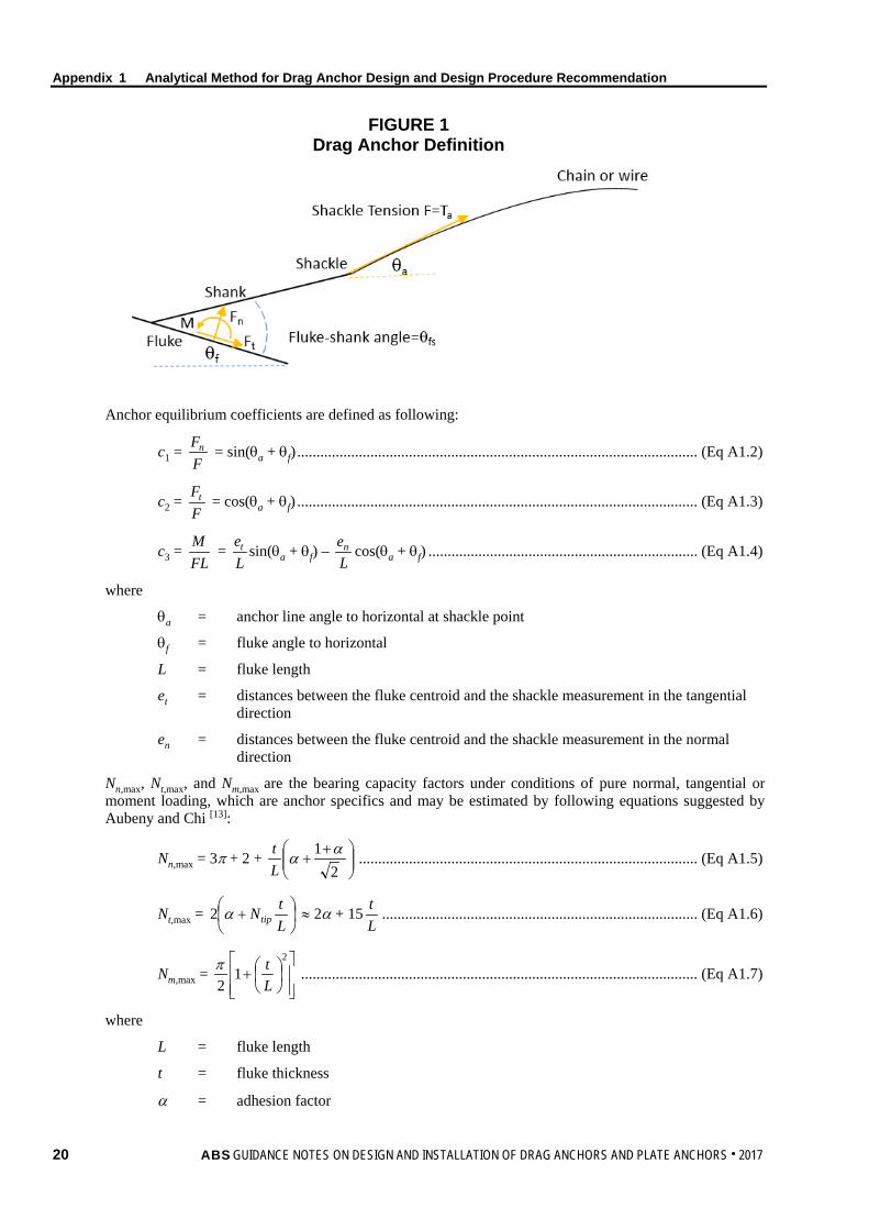
3.1 Anchor Holding Capacity Under Combined Load Drag anchors are generally subjected to combined normal (Fn), tangential (Ft), and moment loading (M), shown in Appendix 1, Figure 1. Consequently, a framework for characterizing the interaction effects under combined loading is required. A relationship originally proposed by Murff [11] for shallow foundations and subsequently adopted by O’Neill et al [12], Aubeny and Chi [13] characterizes the interaction as follows:
f = pn
t
e
m
m
e
q
n
e
N
Nc
N
Nc
N
Nc
1
max,
2
max,
3
max,
1 ||||||
– 1 = 0 ...................................................... (Eq A1.1)
where
Ne = bearing capacity factor under combined loadings
Nn,max = bearing capacity factor under condition of pure normal loading
Nt,max = bearing capacity factor under condition of pure tangential loading
Nm,max = bearing capacity factor under condition of pure moment loading
n, m, p, q = interaction coefficients
c1, c2, c3 = anchor equilibrium coefficients
Appendix 1 Analytical Method for Drag Anchor Design and Design Procedure Recommendation
FIGURE 1 Drag Anchor Definition
Anchor equilibrium coefficients are defined as following:
c1 = FFn = sin(θa + θf) ........................................................................................................ (Eq A1.2)
c2 = FFt = cos(θa + θf) ........................................................................................................ (Eq A1.3)
c3 = FLM =
Let sin(θa + θf) –
Len cos(θa + θf) ...................................................................... (Eq A1.4)
where
θa = anchor line angle to horizontal at shackle point
θf = fluke angle to horizontal
L = fluke length
et = distances between the fluke centroid and the shackle measurement in the tangential direction
en = distances between the fluke centroid and the shackle measurement in the normal direction
Nn,max, Nt,max, and Nm,max are the bearing capacity factors under conditions of pure normal, tangential or moment loading, which are anchor specifics and may be estimated by following equations suggested by Aubeny and Chi [13]:
Nn,max = 3π + 2 +
++
21 αα
Lt ........................................................................................ (Eq A1.5)
Nt,max =
+
LtNtipα2 ≈ 2α + 15
Lt .................................................................................. (Eq A1.6)
Nm,max =
+
2
12 L
tπ ....................................................................................................... (Eq A1.7)
where L = fluke length
t = fluke thickness
α = adhesion factor
20 ABS GUIDANCE NOTES ON DESIGN AND INSTALLATION OF DRAG ANCHORS AND PLATE ANCHORS . 2017

Appendix 1 Analytical Method for Drag Anchor Design and Design Procedure Recommendation
Typical suggested values are 10-12 for Nn,max, 2-4 for Nt,max and 1.6 for Nm,max.
Appropriate values of the interaction coefficients n, m, p and q are typically estimated by fitting Eq A1.1 to finite element calculations or experimental data of ultimate capacity of the fluke under combined loading conditions. In lieu of finite element analyses, or testing, the following coefficients suggested by Murff et al [14] may be used.
TABLE 1 Values of Interaction Coefficient
Exponent Value m 1.56 n 4.19 p 1.57 q 4.43
The bearing capacity factor for anchor under combined loads can be taken as the root of the Eq A1.1. Then anchor holding capacity can be obtained as follows:
Ranchor = NesuAf .................................................................................................................... (Eq A1.8)
where
Ne = bearing capacity factor under combined loadings
su = undrained shear strength of soil at the depth of anchor fluke
Af = area of anchor fluke
It is to be noted that Eq A1.1 does not consider soil resistance acting on the anchor shank. For designs involving thin shanks, such as a bridle system this assumption is reasonable. However, some anchor designs have shank of substantial thickness. The predicted anchor holding capacity may be conservative.
3.3 Kinematic Behavior During drag embedment, the relative magnitudes of translational and rotational motions are of particular importance. Assuming an associated flow law, the angular, tangential and normal velocity of the fluke, β , vt, and vn can be computed by taking appropriate partial derivatives of f (Eq A1.1).
β = λmN
f∂∂ ........................................................................................................................ (Eq A1.9)
vn = λnN
f∂∂ ....................................................................................................................... (Eq A1.10)
vt = λtN
f∂∂ ......................................................................................................................... (Eq A1.11)
where
λ = scalar multiplier
The ratio of rotation to tangential translation, Rrt, is therefore:
Rrt = t
f
vLβ
= 1
max
1
max
max
max
3
3
||
||
|| −
−
n
t
t
m
m
m
m
t
NN
NN
NN
nm
cc
...................................................................... (Eq A1.12)
ABS GUIDANCE NOTES ON DESIGN AND INSTALLATION OF DRAG ANCHORS AND PLATE ANCHORS . 2017 21

Appendix 1 Analytical Method for Drag Anchor Design and Design Procedure Recommendation
The ratio of normal to tangential translation, Rnt, is computed as follows:
Rnt = t
n
vv = 1
max
1
max
11
maxmax
max
max
||
||
||||−
−
−
+
n
t
t
q
n
n
pn
t
tm
m
m
n
t
NN
NN
NN
NN
npq
NN
................................................. (Eq A1.13)
3.5 Embedded Anchor Line Equilibrium Equation In order to predict the trajectory of the anchor as drag embedment progresses, it is necessary to consider the mechanics of the anchor line in addition to those of the anchor itself. The key equation is the relationship between anchor line tension and line angle at the pad-eye formulated by Neubecker and Randolph [15]:
Ta ( )20
2 θ−θa = 2zEnNcb
+
20zksu .................................................................................. (Eq A1.14)
where
Ta = anchor line tension at shackle point
θa = anchor line angle from horizontal at shackle point
θ0 = angle of anchor line from horizontal at mudline
En = multiplier to be applied to chain bar diameter, if applicable (typical = 2.5, for wire line = 1)
Nc = bearing factor for wire anchor line
b = chain bar or wire diameter
su0 = soil undrained shear strength at mudline
k = soil strength gradient with respect to depth
z = depth of shackle below mudline
For convenient recursive calculations of anchor trajectory, Eq A1.13 can be reformulated as follows:
dzd aθ
=
( )
( )
θθ
−θ−θ
θ+
θθ
θ−θ
+θ−θ
−
a
sa
as
e
eaa
u
a
fe
cn
dd
ddN
Ndd
kkzsAN
bNE
12
1
2
20
20
0
0
20
2
................................................... (Eq A1.15)
22 ABS GUIDANCE NOTES ON DESIGN AND INSTALLATION OF DRAG ANCHORS AND PLATE ANCHORS . 2017
Appendix 1 Analytical Method for Drag Anchor Design and Design Procedure Recommendation
5 Simplified Analysis for Trajectory Prediction Both Eq A1.1 and Eq A1.13 give the relationship of tension, Ta, and anchor line angle, θa. The intersection of the two loci produces a unique solution (Ta,θa) for the anchor line tension and angle at a given depth in the trajectory. The subsequent computations of (Ta,θa) as the anchor traverses through its trajectory is produced by the recursive algorithm. However, this trajectory computation procedure is complex and not easily programmed. Moreover, the analysis requires a complete definition of the anchor load capacity curve, which is not easily obtained in most practical cases. Analytical studies by Aubeny and Chi [13] indicate that during drag embedment the anchor tends toward a condition of zero rotation rate relative to the anchor line at the padeye (i.e., the angles θas and θaf are essentially constant throughout drag embedment. Since the load angle is constant throughout dragging, the bearing factor Ne is also constant. It is also shown that these constant values correspond to an equilibrium state for the anchor where the rate of rotation is approximately β = 0.
The following conclusions can be obtained from these findings. Firstly, the orientation of the anchor from the anchor line is always known and can be denoted at the equilibrium angle for the anchor θase. Secondly, a single bearing factor governs anchor behavior during drag embedment, which is denoted the equilibrium bearing factor, Ne. Since the equilibrium bearing factor is known and is constant, it is not necessary to compute the intersection of the anchor capacity curve and the anchor line equation. Thirdly, Eq A1.14 can be simplified as follows:
dzd aθ
=
( )
θθ
θ−θ
+θ−θ
−
aa
u
a
fe
cn
dd
kkzsAN
bNE
00
0
20
2
2 .................................................................................... (Eq A1.16)
7 Procedure The simplified analysis proceeds according to the following steps, see flowchart in Appendix 1, Figure 2:
1. The analysis is initialized by embedding the anchor shackle depth to an arbitrary small, non-zero initial depth, z0. Corresponding to this initial embedment is an initial anchor line angle at the pad-eye, θa0, that is calculated using Eq A1.14. The anchor is assumed to immediately migrate to its equilibrium configuration; that is, the angle between anchor line and the fluke is the equilibrium angle, θafe. The initial fluke orientation θf0 can be computed based on the values for the anchor line angle, θa0, and the angle between the anchor line and the fluke, θafe.
2. To analyze the next step in the anchor trajectory, the anchor is advanced a short incremental distance ∆t in a direction parallel to the fluke.
3. Accompanying this tangential translation, a movement ∆n normal to the fluke can be computed by Eq A1.13 or imposed based on empirical data.
4. The shackle will translate the following incremental distances as described by Eq A1.17 and Eq A1.18, which are repeated here:
∆x = ∆t cos θf + ∆n sin θf .................................................................................... (Eq A1.17)
∆z = ∆t sin θf – ∆n cos θf ..................................................................................... (Eq A1.18)
5. Accompanying this tangential translation will be an anchor rotation computed by Eq A1.16.
6. Steps 2 to 5 are repeated until the analysis has proceeded to the desired drag distance, xmax.
ABS GUIDANCE NOTES ON DESIGN AND INSTALLATION OF DRAG ANCHORS AND PLATE ANCHORS . 2017 23
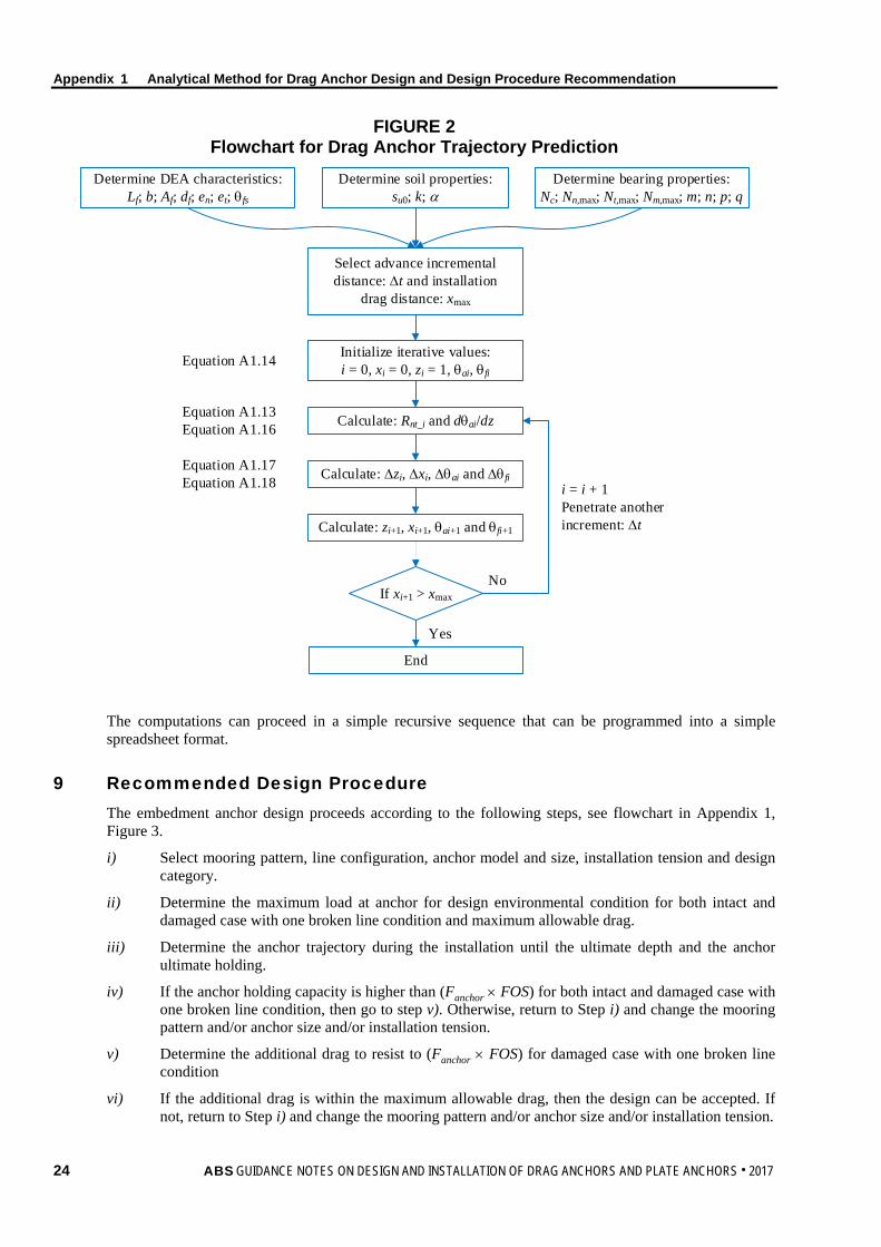
Appendix 1 Analytical Method for Drag Anchor Design and Design Procedure Recommendation
FIGURE 2 Flowchart for Drag Anchor Trajectory Prediction
Determine DEA characteristics:Lf; b; Af; df; en; et; θfs
Determine soil properties:su0; k; α
Determine bearing properties:Nc; Nn,max; Nt,max; Nm,max; m; n; p; q
Select advance incremental distance: ∆t and installation
drag distance: xmax
Initialize iterative values:i = 0, xi = 0, zi = 1, θai, θfi
Calculate: Rnt_i and dθai/dz
Calculate: ∆zi, ∆xi, ∆θai and ∆θfi
Calculate: zi+1, xi+1, θai+1 and θfi+1
If xi+1 > xmax
End
Equation A1.14
Equation A1.13Equation A1.16
Equation A1.17Equation A1.18 i = i + 1
Penetrate another increment: ∆t
No
Yes
The computations can proceed in a simple recursive sequence that can be programmed into a simple spreadsheet format.
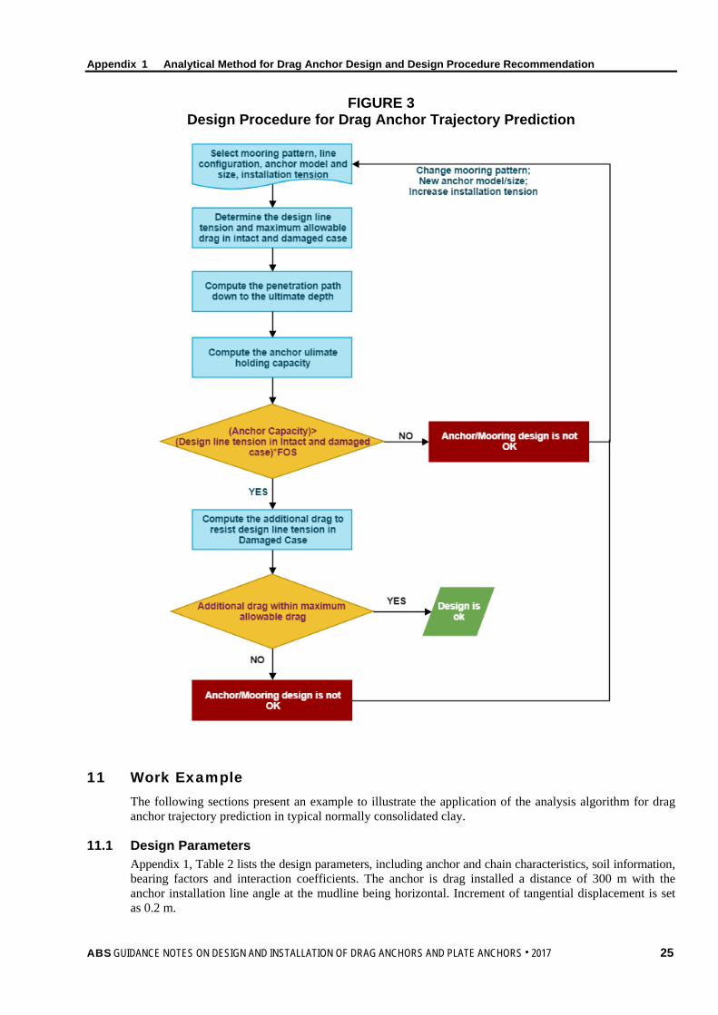
9 Recommended Design Procedure The embedment anchor design proceeds according to the following steps, see flowchart in Appendix 1, Figure 3.
i) Select mooring pattern, line configuration, anchor model and size, installation tension and design category.
ii) Determine the maximum load at anchor for design environmental condition for both intact and damaged case with one broken line condition and maximum allowable drag.
iii) Determine the anchor trajectory during the installation until the ultimate depth and the anchor ultimate holding.
iv) If the anchor holding capacity is higher than (Fanchor × FOS) for both intact and damaged case with one broken line condition, then go to step v). Otherwise, return to Step i) and change the mooring pattern and/or anchor size and/or installation tension.
v) Determine the additional drag to resist to (Fanchor × FOS) for damaged case with one broken line condition
vi) If the additional drag is within the maximum allowable drag, then the design can be accepted. If not, return to Step i) and change the mooring pattern and/or anchor size and/or installation tension.
24 ABS GUIDANCE NOTES ON DESIGN AND INSTALLATION OF DRAG ANCHORS AND PLATE ANCHORS . 2017
Appendix 1 Analytical Method for Drag Anchor Design and Design Procedure Recommendation
FIGURE 3 Design Procedure for Drag Anchor Trajectory Prediction
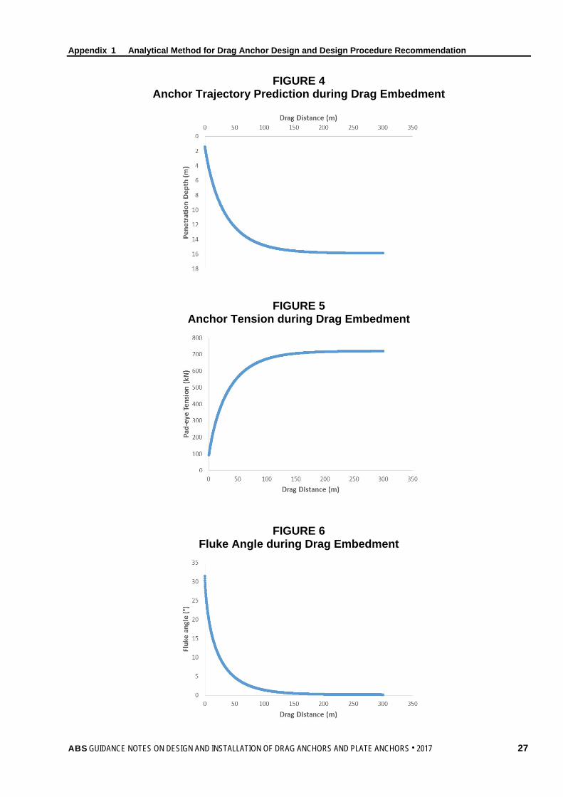
11 Work Example The following sections present an example to illustrate the application of the analysis algorithm for drag anchor trajectory prediction in typical normally consolidated clay.
11.1 Design Parameters Appendix 1, Table 2 lists the design parameters, including anchor and chain characteristics, soil information, bearing factors and interaction coefficients. The anchor is drag installed a distance of 300 m with the anchor installation line angle at the mudline being horizontal. Increment of tangential displacement is set as 0.2 m.
ABS GUIDANCE NOTES ON DESIGN AND INSTALLATION OF DRAG ANCHORS AND PLATE ANCHORS . 2017 25

Appendix 1 Analytical Method for Drag Anchor Design and Design Procedure Recommendation
TABLE 2 Design Parameter for Drag Anchor Trajectory Prediction
Category Parameter Symbol Units Value
Anchor/chain
Fluke area Af m2 6 Fluke length L m 2 Fluke thickness T m 0.3 Line diameter b m 0.073 Fluke-shank angle θfs ° 45
Chain multiplier En --- 1
Bearing factor
Line bearing factor Nc --- 12
Tangential bearing factor Nt,max --- 2.9
Normal bearing factor Nn,max --- 11.6
Moment bearing factor Nm,max --- 1.6
Combined loading interaction coefficient
Interaction coefficient m --- 1.56 Interaction coefficient n --- 4.19 Interaction coefficient p --- 1.57 Interaction coefficient q --- 4.43
Soil Mudline strength su0 kPa 1.5 Strength gradient k kPa/m 1.75 Adhesion factor α --- 0.3
Initial and loading condition
Initial embedment z0 m 1
Initial position x0 m 0
Installation mudline angle θ0 ° 0 Maximum allowable drag (broken line condition)
xallow m 60
maximum load at anchor (intact condition) F kN 450
maximum load at anchor (broken line condition) F kN 645
Discretization Increment of tangential displacement ∆t m 0.2
11.3 Predicted Anchor Trajectory and Holding Capacity Appendix 1, Figures 4 and 5 show predicted drag anchor trajectory and anchor pad-eye tension during anchor embedment. The drag anchor arrives at its ultimate penetration depth (zult = 15.9 m) at the drag distance of about 240 m and the anchor is rotated from fluke angle 31.9° to 0°. The holding capacity of the drag anchor is therefore 720 kN at that depth. As mentioned in Section 2, the analysis does not take shank resistance into account, which produces a conservative result.
11.5 Anchor Design Factors of safety for both intact and broken line extreme conditions are 1.6 and 1.1, respectively. These values are higher than the required value in Appendix 7, Table 1. The potential addition drag in the broken line condition could be obtained from Appendix 1, Figure 5. From line tension 450 kN to 645 kN, the additional drag is 51.6 m, which is within the maximum allowable drag. Thus, the anchor design is acceptable.
26 ABS GUIDANCE NOTES ON DESIGN AND INSTALLATION OF DRAG ANCHORS AND PLATE ANCHORS . 2017
Appendix 1 Analytical Method for Drag Anchor Design and Design Procedure Recommendation
FIGURE 4 Anchor Trajectory Prediction during Drag Embedment
FIGURE 5 Anchor Tension during Drag Embedment
FIGURE 6 Fluke Angle during Drag Embedment
ABS GUIDANCE NOTES ON DESIGN AND INSTALLATION OF DRAG ANCHORS AND PLATE ANCHORS . 2017 27
A p p e n d i x 2 : C y c l i c L o a d i n g E f f e c t
A P P E N D I X 2 Cyclic Loading Effect
1 General The anchoring systems have to withstand severe cyclic loadings from the wind in additions to the wave loading acting on the floating structures. Cyclic loading will influence the strength and stiffness of the soil. As a result, the anchoring systems design should consider the effect of cyclic loading.
Cyclic loading tends to affect the soil’s undrained shear strength in two ways. First, cyclic loadings generally trend to break down the soil structure and thus degrade strength. Secondly, there can be an increase in the soil’s undrained shear strength due to the high loading rate from wave frequency load cycles compared with the monotonic load. The first effect is most pronounced when the soil is subjected to two-way cyclic loadings (with load reversals) and increases with increasing over consolidation ratio of the soil. Since the mooring line is always in tension (no load reversals), the degradation effect on the shear strength is less. The soil undrained shear strength is mostly increased by the net effect of cyclic loading. In soft clay, cyclic loading will also improve the capacity by further penetration of the anchor.
In order to consider these cyclic loading effects in the anchor design, the cyclic shear strength should be determined. This appendix presents recommendations on cyclic loading effect assessment on soil design parameters adopted in Sections 3 and 4. The anchor holding capacity should be calculated using the cyclic shear strength.
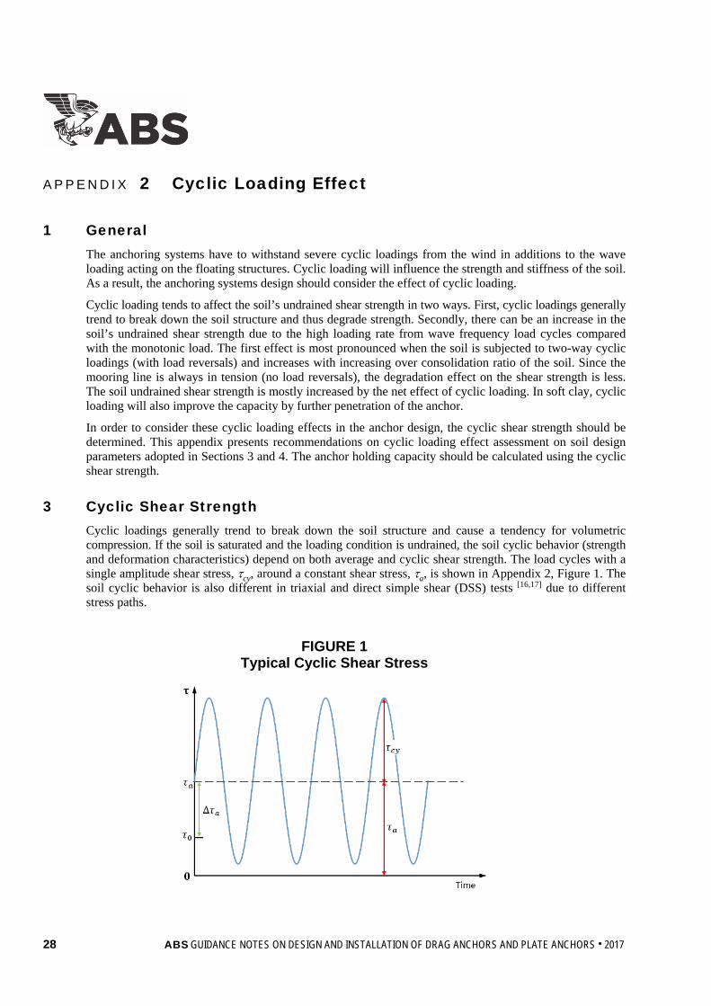
3 Cyclic Shear Strength Cyclic loadings generally trend to break down the soil structure and cause a tendency for volumetric compression. If the soil is saturated and the loading condition is undrained, the soil cyclic behavior (strength and deformation characteristics) depend on both average and cyclic shear strength. The load cycles with a single amplitude shear stress, τcy, around a constant shear stress, τa, is shown in Appendix 2, Figure 1. The soil cyclic behavior is also different in triaxial and direct simple shear (DSS) tests [16,17] due to different stress paths.
FIGURE 1 Typical Cyclic Shear Stress
28 ABS GUIDANCE NOTES ON DESIGN AND INSTALLATION OF DRAG ANCHORS AND PLATE ANCHORS . 2017

Appendix 2 Cyclic Loading Effect
The cyclic shear strength, τf,cy, is defined as the maximum shear stress that can be mobilized during the cyclic loading and it can be determined from the following equation [18]:
τf,cy = (τa + τcy)f ................................................................................................................... (Eq A2.1)
where
(τa + τcy)f = sum of the average and cyclic shear stress at failure
τa = average shear stress
τcy = cyclic shear stress amplitude
The average shear stress, τa, is calculated as follows:
τa = τ0 + ∆τa ........................................................................................................................ (Eq A2.2)
where
τ0 = initial soil shear stress prior to the installation of anchor
∆τa = addition soil shear stress induced by submerged weight of anchor and/or average environmental loads
The cyclic shear strength depends on average shear stress, τa, and the cyclic loading history (i.e., number and magnitude of load cycles, load frequency). It also depends on soil type, plasticity (for clay), density (for sand) and over-consolidation ratio. The cyclic shear strength can be determined from a contour diagram where the cyclic strengths at failure are given as functions of average and cyclic shear stress and number of cycles. This cyclic contour diagram concept has been adopted in offshore foundation design for many years [19,20].
In multiple layers of soil, hard clay, dense sand, cemented carbonate sand, coral or rock, etc., there is no mature methodology to predict the anchor penetration depth and resistance. In such soils or for anchor tip penetration less than one or two fluke width, it is not rational to consider the soil cyclic loading effects.
5 Procedure
5.1 Design Storm Composition and Cycle Counting The cyclic contour diagram is valid for the constant cyclic shear stress condition. However, in the cyclic design, the cyclic load varies from one cycle to the next (irregular loading history). In order to adopt the cyclic contour diagram, the irregular loading history needs to be transformed into a number of parcels with different constant cyclic loads.
The irregular design cyclic load history can be transformed into parcels of constant cyclic load as summarized in Appendix 2, Figure 2 by using the “rain flow” method (ASTM E1049085).
ABS GUIDANCE NOTES ON DESIGN AND INSTALLATION OF DRAG ANCHORS AND PLATE ANCHORS . 2017 29

Appendix 2 Cyclic Loading Effect
FIGURE 2 Example of Transformation of Cyclic Loading History to Constant Cyclic Parcels
No of cycles, N Cyclic load in percentage of max. cyclic load (%)
1 100
1 96
2 90
4 80
30 70
92 60
175 50
340 40
542 30
5.3 Equivalent Number of Cycles to Failure The effect of irregular cyclic loading can be taken into account by determining the equivalent number of cycles of the maximum load, Neq. The equivalent number of cycles, Neq, is defined as the number of cycles of the maximum load that give the same cyclic effect as the real irregular cyclic load history. Neq can be determined either by the pore pressure accumulation procedure [20] or the strain accumulation procedure [22] depending on the soil’s characteristics. The pore pressure accumulation procedure is the preferred procedure in cases where there is possible drainage during the cyclic load history, whereas the strain accumulation procedure may be more suited for clay soils [23].
5.5 Cyclic Contour Diagram The Contour Diagram provides a practical design basis of an offshore foundation. More details on how to construct the contour diagram and the consideration on the testing strategy can be found in the recent findings by Andersen [23]. It is recommend to acquire site specific soil cyclic test data to construct the contour diagram. If relevant cyclic test data for the site is not available, the designer should be conservative in the assessment of cyclic shear strength. The strength and plasticity properties of the clay, relative density and grain size distribution of the sand should be evaluated and compared with the available database. Databases with parameters for cyclic loading of clay are available for Drammen Clay [18,24], Troll Clay [25], and Gulf of Mexico Clay [26,27].
5.7 Description of Procedure The following approach can be used to establish the permissible value of cyclic shear strength, τf,cy:
1. From the irregular design cyclic load history, determine parcels of different constant cyclic loads using the rain flow method.
2. Determine the equivalent number of cycles to failure, Neq; following either the pore pressure accumulation procedure or the strain accumulation procedure, whichever is more suitable.
3. Obtain τa/su from the mooring line analysis through Eq A2.3 below:
u
a
sτ =
fs
a
PP
, ........................................................................................................... (Eq A2.3)
where
Pa = average load
Ps,f = reference monotonic (static) capacity
30 ABS GUIDANCE NOTES ON DESIGN AND INSTALLATION OF DRAG ANCHORS AND PLATE ANCHORS . 2017

Appendix 2 Cyclic Loading Effect
4. Construct the cyclic contour diagram using site specific cyclic test data, supplemented with appropriate empirical data from recognized databases.
5. Determine cyclic shear strength, τf,cy, using contour diagram.
For drag anchor, the anchor holding capacity considered the cyclic loading effect can be calculated by equation:
Ranchor,cyc = Ranchor ×
−+
u
ucyf
ss,1
τ .................................................................................. (Eq A2.4)
where
Ranchor = anchor holding capacity
τf,cy = soil cyclic shear strength
su = soil undrained shear strength
For plate anchor, the anchor holding capacity considered the cyclic loading effect can be calculated by Eq 4.5 in 4/4.3 using τf,cy.
ABS GUIDANCE NOTES ON DESIGN AND INSTALLATION OF DRAG ANCHORS AND PLATE ANCHORS . 2017 31
32 ABS GUIDANCE NOTES ON DESIGN AND INSTALLATION OF DRAG ANCHORS AND PLATE ANCHORS . 2017
A p p e n d i x 3 : S e t - u p E f f e c t
A P P E N D I X 3 Set-up Effect
The soil in the vicinity of the anchor will be disturbed during installation. The shear strength of the soil in the vicinity of the anchor will gradually increase with time due to the combination of thixotropy and consolidation after the installation. Hence, the capacity of the drag anchor and plate anchor will increase with time. The increase in the anchor holding capacity depends on anchor characteristics, the soil properties and time after the installation.
For drag anchors and drag-in plate anchors, the soil being remolded during the penetration path may not affect the anchor holding capacity. Hence the consolidation of this volume of clay will have little or no effect on the holding capacity of the anchor. However, the consolidation of this volume of clay may be considered when the anchor installation is delayed and restart again. For plate anchors, the keying of the plate anchor will lead to a more significant soil disturbance than during penetration.
The thixotropy can be defined as a process of softening caused by remolding, followed by a time dependent return to the original harder state at a constant water contend and constant porosity [28]. The thixotropy effect tends to dominate during the first few days or weeks until the consolidation effect takes over. The ratio between the shear strength after a certain time with thixotropic strength gain and the shear strength just after remolding is referred to as the “thixotropy strength factor”. Jeanjean et al. [29] give upper and lower bound values of the thixotropy factor as function of time and plasticity. However, if the thixotropy effect is significant in the design, laboratory testing for the site specific soil should be considered.
After the installation of the drag anchor and plate anchor, the dissipation of excess pore pressures with time leads to an increase in effective stresses, resulting a higher anchor holding capacity. The soil resistance will be governed by the remolded undrained shear strength, which is depend on the soil sensitivity.
su,r = t
u
s
s ............................................................................................................................. (Eq A3.1)
where
su,r = remolded undrained shear strength
su = undisturbed undrained shear strength
st = soil sensitivity
For a particular anchor and penetration depth, the effect of consolidation depends on the consolidation factor, which is a function of time, soil sensitivity, and soil consolidation characteristics. Test data is necessary to evaluate the effect of anchor consolidation. Based on the experience by Vryholf [4], a typical set-up effect factor is approximately 1.5 for anchors used for drilling rigs for a 3 to 4 week consolidation time.
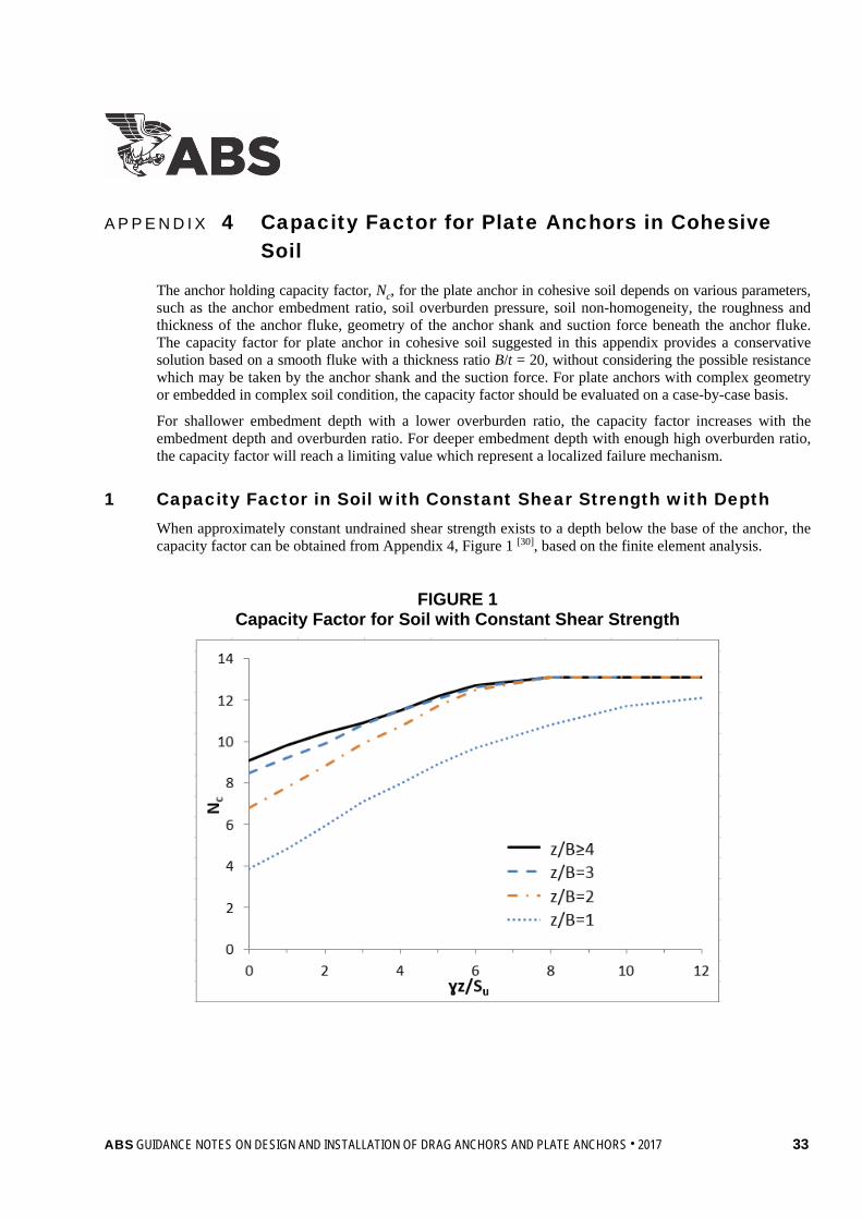
A p p e n d i x 4 : C a p a c i t y F a c t o r f o r P l a t e A n c h o r s i n C o h e s i v e S o i l
A P P E N D I X 4 Capacity Factor for Plate Anchors in Cohesive Soil
The anchor holding capacity factor, Nc, for the plate anchor in cohesive soil depends on various parameters, such as the anchor embedment ratio, soil overburden pressure, soil non-homogeneity, the roughness and thickness of the anchor fluke, geometry of the anchor shank and suction force beneath the anchor fluke. The capacity factor for plate anchor in cohesive soil suggested in this appendix provides a conservative solution based on a smooth fluke with a thickness ratio B/t = 20, without considering the possible resistance which may be taken by the anchor shank and the suction force. For plate anchors with complex geometry or embedded in complex soil condition, the capacity factor should be evaluated on a case-by-case basis.
For shallower embedment depth with a lower overburden ratio, the capacity factor increases with the embedment depth and overburden ratio. For deeper embedment depth with enough high overburden ratio, the capacity factor will reach a limiting value which represent a localized failure mechanism.
1 Capacity Factor in Soil with Constant Shear Strength with Depth When approximately constant undrained shear strength exists to a depth below the base of the anchor, the capacity factor can be obtained from Appendix 4, Figure 1 [30], based on the finite element analysis.
FIGURE 1 Capacity Factor for Soil with Constant Shear Strength
ABS GUIDANCE NOTES ON DESIGN AND INSTALLATION OF DRAG ANCHORS AND PLATE ANCHORS . 2017 33
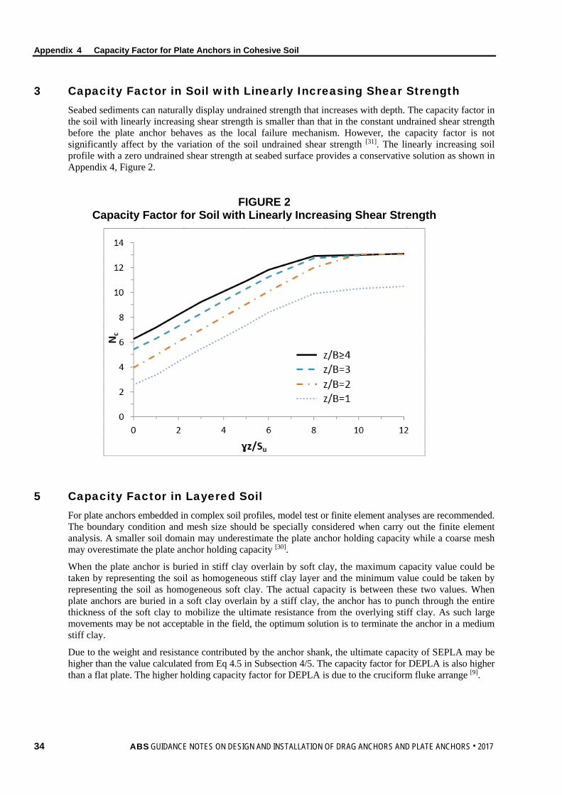
Appendix 4 Capacity Factor for Plate Anchors in Cohesive Soil
3 Capacity Factor in Soil with Linearly Increasing Shear Strength Seabed sediments can naturally display undrained strength that increases with depth. The capacity factor in the soil with linearly increasing shear strength is smaller than that in the constant undrained shear strength before the plate anchor behaves as the local failure mechanism. However, the capacity factor is not significantly affect by the variation of the soil undrained shear strength [31]. The linearly increasing soil profile with a zero undrained shear strength at seabed surface provides a conservative solution as shown in Appendix 4, Figure 2.
FIGURE 2 Capacity Factor for Soil with Linearly Increasing Shear Strength
5 Capacity Factor in Layered Soil For plate anchors embedded in complex soil profiles, model test or finite element analyses are recommended. The boundary condition and mesh size should be specially considered when carry out the finite element analysis. A smaller soil domain may underestimate the plate anchor holding capacity while a coarse mesh may overestimate the plate anchor holding capacity [30].
When the plate anchor is buried in stiff clay overlain by soft clay, the maximum capacity value could be taken by representing the soil as homogeneous stiff clay layer and the minimum value could be taken by representing the soil as homogeneous soft clay. The actual capacity is between these two values. When plate anchors are buried in a soft clay overlain by a stiff clay, the anchor has to punch through the entire thickness of the soft clay to mobilize the ultimate resistance from the overlying stiff clay. As such large movements may be not acceptable in the field, the optimum solution is to terminate the anchor in a medium stiff clay.
Due to the weight and resistance contributed by the anchor shank, the ultimate capacity of SEPLA may be higher than the value calculated from Eq 4.5 in Subsection 4/5. The capacity factor for DEPLA is also higher than a flat plate. The higher holding capacity factor for DEPLA is due to the cruciform fluke arrange [9].
34 ABS GUIDANCE NOTES ON DESIGN AND INSTALLATION OF DRAG ANCHORS AND PLATE ANCHORS . 2017

ABS GUIDANCE NOTES ON DESIGN AND INSTALLATION OF DRAG ANCHORS AND PLATE ANCHORS . 2017 35
A p p e n d i x 5 : L o s s o f E m b e d m e n t D u r i n g K e y i n g f o r S E P L A
A P P E N D I X 5 Loss of Embedment During Keying for SEPLA
The loss of anchor embedment (vertical displacement of the anchor) during keying will be affected by multiple parameters, including the anchor eccentricity (the normal distance from the padeye to the anchor fluke), pullout angle, the anchor fluke thickness, the anchor weight and the soil properties.
An empirical formula [32] can be applied to estimate the loss of anchor embedment:
B
z =
21.0
03.0
2sin
15.0
uf BsA
M
B
t
B
e ..................................................................... (Eq A5.1)
M0 = (f + aW )e – fef + aW ew .............................................................................................. (Eq A5.2)
where
z = loss of anchor embedment
B = width of the anchor fluke
e = loading eccentricity
t = thickness of the anchor fluke
su = soil undrained shear strength at the anchor fluke
= load inclination during the keying
M0 = initial moment corresponding to zero net vertical load on the anchor
Af = area of the anchor fluke
f = anchor shank resistance
aW = difference between the anchor weight in air and the anchor buoyancy force in soil
ef = loading eccentricity for friction resistance
ew = loading eccentricity for anchor weight
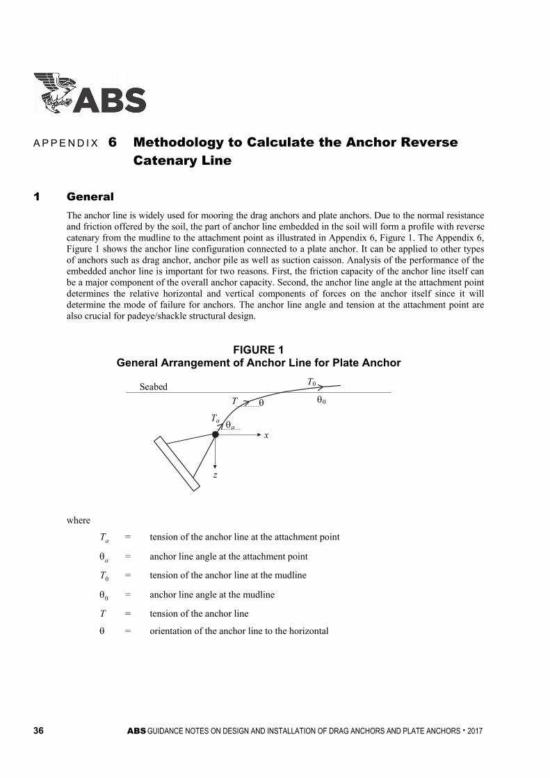
36 ABS GUIDANCE NOTES ON DESIGN AND INSTALLATION OF DRAG ANCHORS AND PLATE ANCHORS . 2017
A p p e n d i x 6 : M e t h o d o l o g y t o C a l c u l a t e t h e A n c h o r R e v e r s e C a t e n a r y L i n e
A P P E N D I X 6 Methodology to Calculate the Anchor Reverse Catenary Line
1 General The anchor line is widely used for mooring the drag anchors and plate anchors. Due to the normal resistance and friction offered by the soil, the part of anchor line embedded in the soil will form a profile with reverse catenary from the mudline to the attachment point as illustrated in Appendix 6, Figure 1. The Appendix 6, Figure 1 shows the anchor line configuration connected to a plate anchor. It can be applied to other types of anchors such as drag anchor, anchor pile as well as suction caisson. Analysis of the performance of the embedded anchor line is important for two reasons. First, the friction capacity of the anchor line itself can be a major component of the overall anchor capacity. Second, the anchor line angle at the attachment point determines the relative horizontal and vertical components of forces on the anchor itself since it will determine the mode of failure for anchors. The anchor line angle and tension at the attachment point are also crucial for padeye/shackle structural design.
FIGURE 1 General Arrangement of Anchor Line for Plate Anchor
T0
T
Ta
0
ax
z
Seabed
where
Ta = tension of the anchor line at the attachment point
a = anchor line angle at the attachment point
T0 = tension of the anchor line at the mudline
0 = anchor line angle at the mudline
T = tension of the anchor line
= orientation of the anchor line to the horizontal

Appendix 6 Methodology to Calculate the Anchor Reverse Catenary Line
3 Equilibrium Equations of Embedded Anchor Line The force equilibrium of an anchor line element is shown in Appendix 6, Figure 2. The differential equations for the embedded section of the anchor line element are:
dsdt = F + w sin θ ................................................................................................................ (Eq A6.1)
Tdsdθ = –Q + w cos θ .......................................................................................................... (Eq A6.2)
where
s = distance measured along the anchor line
F = resistance offered by the soil tangential to the anchor line (per unit length)
w = anchor line self-weight per unit length
Q = resistance offered by the soil normal to the anchor line (per unit length)
FIGURE 2 Force Equilibrium of Anchor Line Element
wds
ds
F
z
x T + dT
θ + dθ
θr
The friction force F on the anchor line is calculated from the following equation [33]:
F = Etdαsu for cohesive soils
F = Etd tan δ for noncohesive soils ............................................................................... (Eq A6.3)
The normal force, Q, on the anchor line is calculated from the following equation:
Q = EndNcsu for cohesive soils
Q = EndNqγ′ z′ for noncohesive soils ............................................................................... (Eq A6.4)
F = µQ ................................................................................................................................ (Eq A6.5)
where Et = multipliers to give the effective widths in the tangential direction, depend on the
configuration of the anchor line, see Appendix 6, Table 1
d = nominal diameter of chain, or diameter of wire or rope.
α = adhesion factor for anchor line
su = undrained shear strength at that position (average, or as measured in simple shear DSSus )
δ = interface friction angle at soil-anchor line interface
ABS GUIDANCE NOTES ON DESIGN AND INSTALLATION OF DRAG ANCHORS AND PLATE ANCHORS . 2017 37

Appendix 6 Methodology to Calculate the Anchor Reverse Catenary Line
En = multipliers to give the effective widths in the normal direction, see Appendix 6, Table 1
Nc = bearing capacity factor, typically in the range of 7.6 to 14, depend on buried depth, shape and orientation, etc.
Nq = bearing capacity factor, depending on the friction angle
= exp(π tan ϕ) tan2(45° + 2ϕ )
γ′ = effective unit weight of the soil
µ = friction coefficient between anchor line and soil, the value should be in the range of 0.4-0.6
z′ = embedment depth of the anchor line from the mudline
TABLE 1 Effective Surface and Bearing Area for Anchor Line
Chain Wire/Rope Et 8-11 π En 2.5 1
5 Simplified Solution for the Mooring Catenary Line The governing equations A6.1 and A6.2 can be solved numerically with an iterative scheme. According to the study by Neubecker and Randolph [33], the self-weight of the anchor line has negligible effect on the chain profile and tension distribution when used in hard soils. The equilibrium equation and the differential equation can be simplified to give the tension profile as:
T = Ta)θθ( −aeµ .................................................................................................................... (Eq A6.6)
( )[ ] aaeTa θθ
)θθ(2 θsinθcos
1µ
µµ +
+− − = ∫ ′
′D
zzQd ................................................................... (Eq A6.7)
For small value of θ, Eq A6.6 may be simplified as:
( )22
2θ−θa
aT = (D – z′)Qave ................................................................................................. (Eq A6.8)
where
D = buried depth of anchor attachment point
Qave = average bearing resistance per unit length of anchor line over the soil depth D
The shape of the reverse catenary line can be derived as:
• For the case of uniform soil, the shape of the reverse catenary line is:
*2*T
x =
+
θ−+
θ *2*1
2* 2
020 zTT ............................................................................ (Eq A6.9)
When θ0 = 0, the equation can be written as:
z* = 2
*2*1
−
Tx ........................................................................................................ (Eq A6.10)
38 ABS GUIDANCE NOTES ON DESIGN AND INSTALLATION OF DRAG ANCHORS AND PLATE ANCHORS . 2017

Appendix 6 Methodology to Calculate the Anchor Reverse Catenary Line
• For the case in which the bearing resistance of the soil increases proportionally with depth (su0 = 0):
Q = kz′ ............................................................................................................................... (Eq A6.11)
The shape of the reverse catenary line is:
**
2 xT
=
( )
+θ
+
+θ
+
220
20
*2**
12*1
ln
zTz
T
.............................................................................. (Eq A6.12)
When θ0 = 0, the equation can be written as:
z* = */2* Txe− ................................................................................................................... (Eq A6.13)
• A general case proposed by Aubeny et al., 2011 [34] for the bearing resistance of the soil increases proportionally with depth (su0 ≠ 0):
x* =
θ++++
θ++++
2/**)(2/*
2/2/ln
21
20221
22212
20221
2212
2 QzQQzQQzQ
QQQQQQQ
....................................... (Eq A6.14)
where
x = horizontal length of the anchor line from anchor
x* = x/D
z* = z′/D
T* = normalized tension
= ave
a
DQT
k = gradient of bearing resistance with depth
su0 = undrain shear strength at mudline
Q1 = normalized soil resistance due to mudline strength
= a
ucn
TDbsNE 0
Q2 = normalized soil resistance due to strength gradient
= a
cn
TbkDNE
2
2
In soft soil with heavy anchor line, the self-weight of the anchor line is balanced by the bearing resistance of the soil. The analytical results can be applied to anchor line with weight by assuming an effective bearing resistance per unit length. Appendix 6 shows the effective bearing resistance profile, Qeff, and the effective embedded depth, Deff.
Qeff, = Q – w ...................................................................................................................... (Eq A6.15)
Deff, = D – δ = D – w/k ...................................................................................................... (Eq A6.16)
ABS GUIDANCE NOTES ON DESIGN AND INSTALLATION OF DRAG ANCHORS AND PLATE ANCHORS . 2017 39
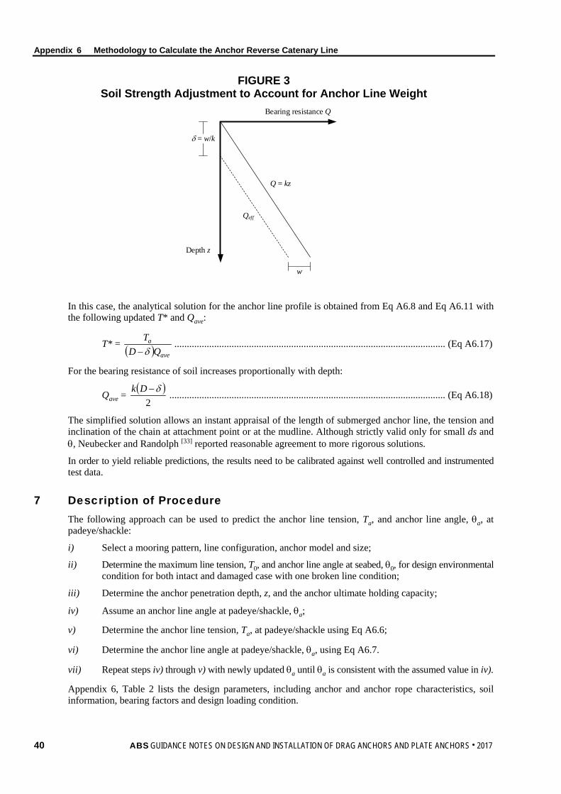
Appendix 6 Methodology to Calculate the Anchor Reverse Catenary Line
FIGURE 3 Soil Strength Adjustment to Account for Anchor Line Weight
w
Q = kz
Qeff
Depth z
δ = w/k
Bearing resistance Q
In this case, the analytical solution for the anchor line profile is obtained from Eq A6.8 and Eq A6.11 with the following updated T* and Qave:
T* = ( ) ave
a
QDTδ−
............................................................................................................. (Eq A6.17)
For the bearing resistance of soil increases proportionally with depth:
Qave = ( )2
δ−Dk ............................................................................................................... (Eq A6.18)
The simplified solution allows an instant appraisal of the length of submerged anchor line, the tension and inclination of the chain at attachment point or at the mudline. Although strictly valid only for small ds and θ, Neubecker and Randolph [33] reported reasonable agreement to more rigorous solutions.
In order to yield reliable predictions, the results need to be calibrated against well controlled and instrumented test data.
7 Description of Procedure The following approach can be used to predict the anchor line tension, Ta, and anchor line angle, θa, at padeye/shackle:
i) Select a mooring pattern, line configuration, anchor model and size;
ii) Determine the maximum line tension, T0, and anchor line angle at seabed, θ0, for design environmental condition for both intact and damaged case with one broken line condition;
iii) Determine the anchor penetration depth, z, and the anchor ultimate holding capacity;
iv) Assume an anchor line angle at padeye/shackle, θa;
v) Determine the anchor line tension, Ta, at padeye/shackle using Eq A6.6;
vi) Determine the anchor line angle at padeye/shackle, θa, using Eq A6.7.
vii) Repeat steps iv) through v) with newly updated θa until θa is consistent with the assumed value in iv).
Appendix 6, Table 2 lists the design parameters, including anchor and anchor rope characteristics, soil information, bearing factors and design loading condition.
40 ABS GUIDANCE NOTES ON DESIGN AND INSTALLATION OF DRAG ANCHORS AND PLATE ANCHORS . 2017
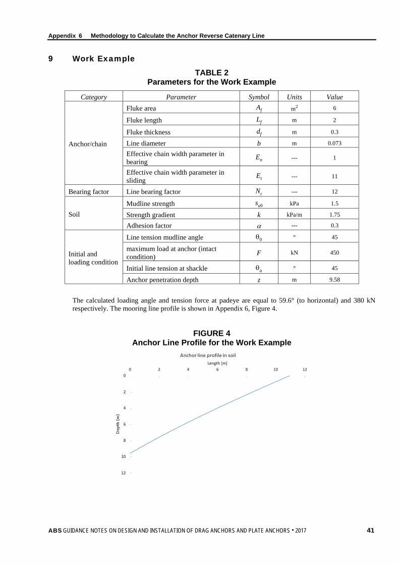
Appendix 6 Methodology to Calculate the Anchor Reverse Catenary Line
9 Work Example
TABLE 2 Parameters for the Work Example
Category Parameter Symbol Units Value
Anchor/chain
Fluke area Af m2 6
Fluke length Lf m 2
Fluke thickness df m 0.3
Line diameter b m 0.073
Effective chain width parameter in bearing
En --- 1
Effective chain width parameter in sliding
Et --- 11
Bearing factor Line bearing factor Nc --- 12
Soil Mudline strength su0 kPa 1.5
Strength gradient k kPa/m 1.75
Adhesion factor α --- 0.3
Initial and loading condition
Line tension mudline angle θ0 ° 45
maximum load at anchor (intact condition) F kN 450
Initial line tension at shackle θa ° 45
Anchor penetration depth z m 9.58
The calculated loading angle and tension force at padeye are equal to 59.6° (to horizontal) and 380 kN respectively. The mooring line profile is shown in Appendix 6, Figure 4.
FIGURE 4 Anchor Line Profile for the Work Example
ABS GUIDANCE NOTES ON DESIGN AND INSTALLATION OF DRAG ANCHORS AND PLATE ANCHORS . 2017 41

A p p e n d i x 7 : C o m m e n t a r y o n A c c e p t a n c e C r i t e r i a
A P P E N D I X 7 Commentary on Acceptance Criteria
1 General The acceptance criteria for drag anchor and plate anchor are specified in 6-1-2/3 of the FPI Rules. This appendix provides the criteria for easy use and reference. Users are advised to check periodically on the ABS website www.eagle.org for the latest version of the FPI Rules.
3 Factor of Safety for Drag anchor The design criterion to be satisfied is:
Ranchor ≥ Fanchor × FOS ........................................................................................................ (Eq A7.1)
where
Fanchor = maximum load at anchor for design environmental condition
FOS = factor of safety (in Appendix 7, Table 1)
TABLE 1 Factor of Safety for Drag anchor Holding Capacities
Condition Factor of safety
Permanent Mobile Intact Design (DEC) 1.5 0.8
Broken Line Extreme (DEC) 1.0 Not required
Note: DEC is the design environmental condition. See 3-2-3/1.1 of the FPI Rules.
The maximum load at anchor, Fanchor, is to be calculated, in consistent units, as follows:
Fanchor = Pline – WsubDwater – Ffriction ..................................................................................... (Eq A7.2)
Ffriction = fslLbedWsub ............................................................................................................. (Eq A7.3)
where
Pline = maximum mooring line tension
Wsub = submerged unit weight of mooring line
Dwater = water depth
Ffriction = friction of mooring line on the sea bed
fsl = frictional coefficient of mooring line on sea bed at sliding
Lbed = length of mooring line on seabed at the design storm condition, not to exceed 20 percent of the total length of a mooring line
42 ABS GUIDANCE NOTES ON DESIGN AND INSTALLATION OF DRAG ANCHORS AND PLATE ANCHORS . 2017
Appendix 7 Commentary on Acceptance Criteria
Note: The above equation for Ffriction is strictly correct only for a single line of constant, Wsub, without buoys or clump weights. Appropriate adjustments will be required for other cases. If uplift angle is considered, Lbed = 0.
The frictional coefficient, fsl, depends on the soil condition and the type of mooring line. For soft mud, sand and clay, the following values [1] of fsl along with the coefficient of friction at start, fsl, for wire rope and chain may be considered representative:
TABLE 2 The Coefficient of Friction for Mooring Line
Coefficient of Friction, f
Starting, fst Sliding, fsl Chain 1.00 0.70
Wire Rope 0.60 0.25
When the soil properties along the embedded anchor line is well known, there is an alternative option for the value of Ffriction in Eq A7.1. It can be applied as the tension force at the anchor attachment point according to the procedure in Appendix 6.
5 Factor of Safety for Plate Anchor The design criterion to be satisfied is:
RPLA ≥ Fanchor × FOS ........................................................................................................... (Eq A7.4)
where
RPLA = holding capacity of plate anchor
Fanchor = maximum load at anchor at design environmental condition
FOS = factor of safety (in Appendix 7, Table 1)
Factors of safety for the anchor holding capacity is defined as the calculated soil resistance divided by the maximum anchor load from dynamic analysis. The factors of safety for plate anchors are listed in Appendix 7, Table 1. It is higher than the factors of safety required for drag anchors due to the difference in failure mechanisms. When a drag anchor reaches its ultimate holding capacity, it will continuously drag through the soil without generating additional holding capacity (i.e., the load will stay equal to the ultimate holding capacity). When a plate anchor exceeds its ultimate pullout capacity, it will slowly be pulled out of the soil.
TABLE 3 Factor of Safety for Plate Anchor
Condition Factor of safety
Permanent Mobile Intact Design (DEC) 2.0 1.5
Broken Line Extreme (DEC) 1.5 1.2
Note: DEC is the design environmental condition. See 3-2-3/1.1 of the FPI Rules.
When the soil properties along the embedded anchor line is well known, there is an alternative option for the value of Ffriction in Eq A7.1. It can be applied as the tension force at the anchor attachment point according to the procedure in Appendix 6.
ABS GUIDANCE NOTES ON DESIGN AND INSTALLATION OF DRAG ANCHORS AND PLATE ANCHORS . 2017 43

Appendix 7 Commentary on Acceptance Criteria
7 Acceptance Criteria for Yielding When the anchors are applied for permanent mooring, the equivalent Von Mises stress generated by applied loads is to be limited to the following stresses for the broken line extreme and intact conditions, respectively.
σeqv ≤ 0.9σyield for broken line extreme condition
σeqv ≤ 0.67σyield for intact condition
where
σeqv = equivalent Von Mises stress
σyield = yield stress of the considered anchor structural component
When the anchors are used for mobile mooring, the allowable stress can be considered following 3-2-1/3.3 of the MODU Rules.
9 Acceptance Criteria for Fatigue Fatigue check is required when the anchors are used for permanent installation. According to the FPI Rules, the anchor structure can be considered as non-inspectable and non-repairable. The safety factors for fatigue life is 10.
44 ABS GUIDANCE NOTES ON DESIGN AND INSTALLATION OF DRAG ANCHORS AND PLATE ANCHORS . 2017
A p p e n d i x 8 : R e f e r e n c e s
A P P E N D I X 8 References
1. API RP 2SK (2005). Recommended practice for design and analysis of stationkeeping systems for floating structures, 3rd Edition, American Petroleum Institute, Washington, D.C.
2. NAVFAC (2012). Naval Facilities Engineering Command. Handbook for Marine Geotechnical Engineering, California.
3. ISO 19901-7 (2013). Stationkeeping systems for floating offshore structures and mobile offshore units, 2nd Edition
4. Vryhof (2015). Anchor Manual 2015. V. Anchors and K. a. Yssel. The Netherlands.
5. Brown, R. P., P. C. Wong and J. M. Audibert (2010). “SEPLA keying prediction method based on full-scale offshore tests.” International Symposium on Frontiers in Offshore Geotechnics(ISFOG). Perth, Western Australia.
6. Gaudin, C., C. D. O'Loughlin and M. F. Randolph (2006a). “Centrifuge tests on suction embedded plate anchors.” the 6th International Conference on Physical Modelling in Geotechnics, Balkema, Rotterdam.
7. Wilde, B., H. Treu and T. Fulton (2001). “Field testing of suction embedded plate anchors.” The 11th International Offshore and Polar Engeering Conference, Stavanger.
8. Gaudin, C., C. D. O'Loughlin, M. F. Randolph and A. C. Lowmass (2006b). “Influence of the installation process on the performance of suction embedded plate anchors.” Geotechnique 56(6): 381-391.
9. O’Loughlin, C. D., Blake, A. P., Richardson, M. D., Randolph, M. F., & Gaudin, C. (2014). “Installation and capacity of dynamically embedded plate anchors as assessed through centrifuge tests.” Ocean Engineering, 88: 204-213.
10. Skempton, A. W. (1951). “The bearing capacity of clays.” Proceeding of the building research congress, London, Vol, 1, pp.180-189.
11. Murff, J. D. (1994). “Limit analysis of multi-footing foundation systems.” Proceedings of the 8th International Conference on Computer Methods and Advances in Geomechanics, Morgantown, West Virginia, 1, 233-244.
12. O’Neill, M.P., Bransby, M.F. & Randolph, M.F. (2003) “Drag anchor fluke-soil interaction in clays,” Can. Geotech. J., 40: 78-94.
13. Aubeny, C. P., and C. Chi. (2009) “Mechanics of drag embedment anchors in a soft seabed.” Journal of geotechnical and geoenvironmental engineering 136.1: 57-68.
14. Murff, J. D., Randolph M. F., Elkhatib, S., Kolk, H. J., Ruionen, R. M., Strom, P. J., and Thorne, C. P. (2005). “Vertically loaded plate anchors for deepwater applications.” Proc. Int. Symp. on Frontiers in Offshore Geotechnics, IS-FOG05, Perth, 31-48.
15. Neubecker, S. R., and Randolph, M. F. (1995). “Profile and frictional capacity of embedded anchor chain,” Journal of Geotechnical Engineering.
16. Andersen, Knut H. (2009) “Bearing capacity under cyclic loading-offshore, along the coast, and on land. The 21st Bjerrum Lecture presented in Oslo, 23 November 2007” Canadian Geotechnical Journal 46.5: 513-535.
17. Andersen, K. H. (2004). Cyclic clay data for foundation design of structures subjected to wave loading. In Proceedings of the International Conference on Cyclic Behaviour of Soils and Liquefaction Phenomena, CBS04, Bochum, Germany (Vol. 31, pp. 371-387).
ABS GUIDANCE NOTES ON DESIGN AND INSTALLATION OF DRAG ANCHORS AND PLATE ANCHORS . 2017 45
Appendix 8 References
18. Andersen, K.H. & Lauritzsen, R. (1988). Bearing capacity for foundations with cyclic loads. ASCE, J. of Geotech. Engrg, 114 (5): 540–555.
19. Andersen, K.H. & Høeg, K. (1991). Deformations of soils and displacements of structures subjected to combined static and cyclic loads. X ECSMFE, Firenze, Proc., (4): 1147–1158.
20. Andersen, K.H., Allard, M.A. & Hermstad, J. (1994). “Centrifuge model tests of a gravity platform on very dense sand; II: Interpretation.” The 7th Int. Conf. on Behavior of Offshore Structures. BOSS’94. Cambridge, Mass. Proc. (1): 255–282.
21. Andersen, K. H., & Jostad, H. P. (1999). “Foundation design of skirted foundations and anchors in clay.” Offshore Technology Conference, Paper OTC 10824.
22. Andersen, K.H. (1976). “Behavior of clay subjected to undrained cyclic loading.” Int. Conf. on Behaviour of OffshStruct., BOSS’76. Trondh. Proc. (1): 392–403. Also NGI Pub. 114.
23. Andersen, K.H. (2015). “Cyclic soil parameters for offshore foundation design.” Frontiers in Offshore Geotechnics: ISFOG, 5-82.
24. Andersen, K.H., A. Kleven and D. Heien. (1988). “Cyclic soil data for design of gravity structures.” Journal of Geotechnical Engineering, ASCE, 114(5): 517-539.
25. By, T. and Skomedal, E. (1992). “Soil parameters for foundation design, Troll platform.” Behaviour of Offshore Structures BOSS'92, pp. 909-920
26. Dutt, R.N., E.H. Doyle and R.S. Ladd. (1992). “Cyclic behaviour of a deepwater normally consolidated clay.” Int. Conf. on Civil Engrg. in the Oceans, Texas, Proc., pp. 546-559
27. Jeanjean. P, Andersen K.H. and Kalsnes B. (1998). “Soil parameters for design of suction caissons for Gulf of Mexico deepwater clays.” Offshore Technology Conference, Paper OTC 8830, pp. 505-519. Houston.
28. Mitchell, J.K. (1960). “Fundamental aspects of thixotropy in soils.” ASCE Journal of Geotechnical Engineering 86(SM3).
29. Jeanjean, P. (2006). “Setup characteristics of suction anchors for soft Gulf of Mexico clays: experience from field installation and retrieval.” OTC18005.
30. Chen, Z., K. K. Tho, C. F. Leung and Y. K. Chow (2013). “Influence of overburden pressure and soil rigidity on uplift behavior of square plate anchor in uniform clay.” Computers and Geotechnics 52: 71-81.
31. Tho, K. K., Z. Chen, C. F. Leung and Y. K. Chow (2014). “Pullout behaviour of plate anchor in clay with linearly increasing strength.” Canadian Geotechnical Journal 51(1): 92-102.
32. Gaudin, C., M. Simkin, D. J. White and C. D. O'Loughlin (2010). “Experimental investigation into the influence of a keying flap on the keying behaviour of plate anchors.” The 20th International Offshore and Polar Engineering Conference, Beijing, China.
33. Neubecker, S.R. and Randolph, M.F. (1995). “Profile and frictional capacity of embedded anchor chains.” Journal of Geotechnical Engineering 121(11): 797-803.
34. Aubeny C, Gilbert R., Randall R., Zimmerman E., McCarthy K., Chen C-H, Aaron D., Yeh P., Chi C-M. and Beemer R. (2011). “The performance of Drag Embedment Anchors (DEA).” Final Project Report, prepared for ABS Consulting, OTRC Project 32558-A6960.
46 ABS GUIDANCE NOTES ON DESIGN AND INSTALLATION OF DRAG ANCHORS AND PLATE ANCHORS . 2017


![DnV-RP-E302 - Design and Installation of Plate Anchors in Clay [2000]](https://img.pdfslide.net/doc/110x75/577ccd5c1a28ab9e788c1d8c/dnv-rp-e302-design-and-installation-of-plate-anchors-in-clay-2000.jpg)