Embed Size (px)
Citation preview
Design, execution and analysisof the livestock breed surveyin Oromiya Regional State, Ethiopia
editors
Workneh Ayalew and J. Rowlands
International Livestock Research InstituteP.O. Box 30709, Nairobi, Kenya
Oromiya Agricultural Development BureauP.O. Box 8770, Addis Ababa, Ethiopia
Project team members:
Anette van Dorland1
John Rowlands2
Asfaw Tolossa3
Edward Rege2
Workneh Ayalew4
Gemechu Degefa4
Markos Tibbo4
Yetnayet Mamo4
Enyew Negussie5
1. International Livestock Research Institute (ILRI), P.O. Box 5689, Addis Ababa,
Ethiopia. Current address: Institut für Nutztierwissenschaften, Tierernährung,
ETH-Zürich, ETH-Zentrum, CH-8092 Zürich
2. ILRI, P.O. Box 30709, Nairobi, Kenya
3. Oromiya Agricultural Development Bureau, P.O. Box 8770, Addis Ababa, Ethiopia
4. ILRI, P.O. Box 5689, Addis Ababa, Ethiopia
5. ILRI, P.O. Box 5689, Addis Ababa, Ethiopia. Current address: MTT Agrifood
Research Finland, Animal Production Research/Animal Breeding, 31600 Jokioinen,
Finland
© 2004 ILRI (International Livestock Research Institute)
All rights reserved. Parts of this publication may be reproduced for non-commercial use
provided that such reproduction shall be subject to acknowledgment of ILRI as holder
of copyright.
ISBN 92–9146–160–1
Correct citation: Workneh Ayalew and Rowlands J. (eds). 2004. Design, execution and
analysis of the livestock breed survey in Oromiya Regional State, Ethiopia. OADB (Oromiya
Agricultural Development Bureau), Addis Ababa, Ethiopia, and ILRI (International
Livestock Research Institute), Nairobi, Kenya. 260 pp.
Table of contentsAcronyms. . . . . . . . . . . . . . . . . . . . . . . . . . . . . . . . . . . . . . . . . . . . . . . . . . . . . . . . . . . . . iv
Acknowledgments . . . . . . . . . . . . . . . . . . . . . . . . . . . . . . . . . . . . . . . . . . . . . . . . . . . . . . v
Foreword . . . . . . . . . . . . . . . . . . . . . . . . . . . . . . . . . . . . . . . . . . . . . . . . . . . . . . . . . . . . . 1
1. Project background and objectives. . . . . . . . . . . . . . . . . . . . . . . . . . . . . . . . . . . . . . . 3
2. Planning and organisation of activities . . . . . . . . . . . . . . . . . . . . . . . . . . . . . . . . . . . 5
3. Development and design of sampling frame . . . . . . . . . . . . . . . . . . . . . . . . . . . . . . . 8
4. Questionnaire design and content. . . . . . . . . . . . . . . . . . . . . . . . . . . . . . . . . . . . . . 15
5. Field work activities . . . . . . . . . . . . . . . . . . . . . . . . . . . . . . . . . . . . . . . . . . . . . . . . . 17
6. Data coding and entry . . . . . . . . . . . . . . . . . . . . . . . . . . . . . . . . . . . . . . . . . . . . . . . 20
7. Survey budget . . . . . . . . . . . . . . . . . . . . . . . . . . . . . . . . . . . . . . . . . . . . . . . . . . . . . 23
8. Population estimation . . . . . . . . . . . . . . . . . . . . . . . . . . . . . . . . . . . . . . . . . . . . . . . 25
9. Descriptive results . . . . . . . . . . . . . . . . . . . . . . . . . . . . . . . . . . . . . . . . . . . . . . . . . . 28
10. Cattle . . . . . . . . . . . . . . . . . . . . . . . . . . . . . . . . . . . . . . . . . . . . . . . . . . . . . . . . . . . . 64
11. Sheep . . . . . . . . . . . . . . . . . . . . . . . . . . . . . . . . . . . . . . . . . . . . . . . . . . . . . . . . . . . 120
12. Goat . . . . . . . . . . . . . . . . . . . . . . . . . . . . . . . . . . . . . . . . . . . . . . . . . . . . . . . . . . . . 172
13. Secondary species . . . . . . . . . . . . . . . . . . . . . . . . . . . . . . . . . . . . . . . . . . . . . . . . . . 222
14. Evaluation of the survey process . . . . . . . . . . . . . . . . . . . . . . . . . . . . . . . . . . . . . . 250
15. Conclusion. . . . . . . . . . . . . . . . . . . . . . . . . . . . . . . . . . . . . . . . . . . . . . . . . . . . . . . 252
iii
AcronymsAEZ Agro-ecological zone
AHC Agglomerative hierarchical clustering
AnGR Animal genetic resources
ARTP Agricultural Research and Training Project
CBPP Contagious bovine pleuro-pneumonia
CCPP Contagious caprine pleuro-pneumonia
DA development agents
EARO Ethiopian Agricultural Research Organization
FAO Food and Agriculture Organization of the United Nations
FMD Foot-and-mouth disease
ha hectare
HH households (number of)
ILRI International Livestock Research Institute
masl metre above sea level
OADB Oromiya Agricultural Development Bureau
OARI Oromiya Agricultural Research Institute
PA Peasant association
PCA Principal component analysis
PPR Peste des petits ruminants
SADC Southern Africa Development Community
sd standard deviation (of the sample)
se standard error (of the mean)
UNDP United Nations Development Programme
iv
AcknowledgementsMany people have contributed to the success of this project. Firstly, we would like to
thank the farmers of Oromiya Regional State who were willing to provide information
on their households and animals. We would also like to thank all the zonal and woreda
livestock experts, together with development agents from the Oromiya agricultural
offices, who conducted the survey.
The research team is also heavily indebted to Mr Asfaw Tolossa of the Oromiya Agri-
cultural Development Bureau (OADB) who served as the main link between the research
team, OADB in Addis Ababa and the field staff of the OADB at zone and district levels
throughout the implementation of this study and without whom this study would not
have been possible.
Dr Edward Rege of the International Livestock Research Institute (ILRI) initiated the
project and provided overall supervision. Dr Enyew Negussie, during his stay at ILRI up
to the middle of 2000, led the first part of the project, which involved the development
of the questionnaires, sampling frame and field co-ordination of the survey. Ms Anette
van Dorland, an Associate Professional Officer at ILRI between 01 April 2000 and 30
April 2003 with support from the Government of The Netherlands, led the second part
of the project, and co-ordinated the remainder of the field data collection, supervised the
data entry and analysed the data on cattle (Chapter 10). At the request of the OADB,
the ILRI team composed of Dr Workneh Ayalew, Mr Gemechu Degefa, Dr Markos
Tibbo and Ms Yetnayet Mamo analysed data on sheep, goats and secondary species and
produced chapters 11, 12 and 13 of this report. Dr John Rowlands provided biometric
assistance at various stages in the process from survey design to report writing.
Finally, our thanks go to Fisseha Teklu, Nigatu Alemayehu, Eshetu Zerihun, Michael
Temesgen, Ewnetu Ermias and a large number of data entry assistants for having contrib-
uted in various ways to the outcome of this study.
The survey fieldwork, analysis and report preparation was funded by OADB from
funds provided by the United Nations Development Programme (UNDP). A reporting
back workshop, on demonstrating the utility of the survey data and its results, was
funded by the Ethiopian Agricultural Research Organization (EARO) through the
Oromiya Agricultural Research Institute (OARI) from the Agricultural Research and
Training Project (ARTP) funds.
v
ForewordThis report presents a comprehensive description of the methods used in the planning,
execution and analysis of the livestock breed survey conducted in the Oromiya Regional
State of Ethiopia between 2000 and 2003, as well as a baseline set of results of data analy-
sis. It has 15 chapters. The first nine chapters describe the background of the study, its
planning and implementation. Chapters 10, 11 and 12, respectively, present results of
the survey on cattle, sheep and goats, which are considered in this survey as primary live-
stock species or entry points for the design and execution of the study. Chapter 13 deals
with secondary species, namely chickens, donkeys, horses, mules and camels, which were
captured in the survey based on consideration of the primary species. Pigs were also in-
cluded in the list of secondary species, but the data generated is too small to be included
in the results as only a handful of households reported maintaining pigs. The last two
chapters present an evaluation of the survey process and concluding remarks. The three
questionnaires developed and administered in this survey are presented in the
accompanying CD-ROM of the report, together with the coat colour chart developed
and successfully used in the survey. The CD-ROM also contains breed descriptors and
outputs of the supervisors training and reporting back workshops.
This livestock breed survey was a collaborative initiative between the Oromiya
Agricultural Development Bureau (OADB) and the International Livestock Research
Institute (ILRI). The United Nations Development Programme (UNDP) funded this
initiative. ILRI took charge of the design, execution and analysis of the data generated in
consultation with OADB. This survey highly benefitted from the experiences in the im-
plementation of a similar livestock survey project, supported by the Food and Agriculture
Organization of the United Nations (FAO) that ILRI undertook in Zimbabwe in collab-
oration with the University of Zimbabwe and the Matapos Research Station. This work
is undertaken as part of ILRI’s continuing research on the characterisation and conserv-
ation of indigenous animal genetic resources with emphasis on providing essential
research tools and building human capacity in collaborating national institutions to
carry out related research as well as development activities.
The survey primarily aims to provide a wide range of baseline data on livestock pro-
duction, mainly cattle, sheep and goats (primary species) but also chickens, donkeys,
horses, mules and camels (secondary species) in Oromiya Regional State. It also aims at
developing and testing a livestock field survey methodology as a tool for breed charac-
terisation. The survey has, however, failed short of identifying the indigenous breed
types of the major livestock species due to unforeseen limitations of the data collected
and especially because of the many ways farmers identify their livestock breed types. An
appropriate statistical procedure was identified and demonstrated on a subset of the data
to help achieve this last objective.
1

Despite a very short planning and implementation time, the survey was generally
implemented successfully, with the key lesson that the time needed for such surveys
should not be underestimated. It is hoped that the baseline information generated can
support future livestock development activities, and the survey tools developed can be
extensively used and adapted for similar purposes in and outside Oromiya Regional
State.
2
1 Project background and objectives1.1 BackgroundOromiya Regional State is Ethiopia’s largest region covering over 30% of the country. It
is characterised by immense geographical and climatic diversity with altitudes ranging
from below 500 metres above sea level (masl) to over 4300 masl. The climatic types pre-
vailing in the region may be grouped into three major categories: dry, tropical rainy, and
temperate rainy climate. Annual rainfall is variable, ranging from 1600–2400 mm in the
highlands and less than 400 mm in the semi-arid lowlands. The diversity in altitudes and
climatic types has resulted in a variety of habitats. The selection pressure of these habitats
on domestic animals, and the human selection for domestic animals suited best for their
needs, has led to the development of a variety of localised livestock breeds and strains.
These breeds/strains or breed types are well adapted to the specific local environments
in which they are kept.
Only limited technical information is available on domestic animal genetic resources
in Oromiya Regional State, and in the country as a whole. There is a need to charac-
terise the diverse livestock breeds/strains, so that action can be taken to develop them,
to meet the current and future demands for animal products, to conserve existing in-
digenous breeds so that genetic diversity is not lost for future generations, and to de-
velop programmes for genetic improvements. Characterisation of domestic animal
genetic resources (AnGR) includes all descriptive features that could be used to provide
better knowledge of the resources and their status (FAO 1999). Characterisation of
domestic AnGR helps to identify breeds and/or populations, along with their specific
traits, which can be used in livestock development programmes. Characterisation can
also identify breeds and/or populations, which are at risk of extinction or breeds that are
highly desired by farmers. Both categories provide important inputs into national live-
stock development planning.
In 2000, in response to the situation described above, the Oromiya Agricultural
Development Bureau (OADB) and the International Livestock Research Institute (ILRI)
undertook the ‘Oromiya–ILRI livestock breed survey’ project to characterise domestic
livestock breeds and their husbandry practices in Oromiya Regional State.
1.2 ObjectivesThe overall objective of the livestock breed survey was to identify and describe the in-
digenous animal genetic resources (AnGR) of Oromiya Regional State and the pro-
duction systems in which they are found. In addition, it aimed to describe the economic,
social and cultural roles of AnGR as well as farmers’ preferences for traits and breeds.
3

The emphasis of the survey was on pure indigenous livestock, but information was also
collected on crosses between indigenous with exotic breeds, as well as on pure exotic
breeds. An additional objective of this study was to assess the suitability of the field
survey methodology and questionnaire design applied as a tool for breed characteris-
ation.
It is hoped that the generated baseline information can support future livestock
development activities, identify possible causes of threat for AnGR and indicate possible
actions to mitigate their impacts.
4
2 Planning and organisation of activities2.1 Planning
The planning and organisation of a livestock breed survey requires careful attention.
Good planning will ultimately result in a good course of events, which in turn will lead
to a good result. From our experience, a period of at least six months should be allowed
for the planning of a survey of this nature. The following activities were undertaken for
the Oromiya Regional State survey:
• preliminary planning meetings, seeking collaborators and agreeing on the objectives
of the survey
• establishment of guidelines for administration and organisation, making decisions on
how to implement the survey activities and on who should be involved in doing what
• survey design planning and preparation, including: 1) collecting information on
households, animal numbers etc. to assist in the planning and preparation of the
survey design; 2) preparing survey sampling frame; 3) preparing survey materials and
questionnaires, instruction manuals, descriptor lists, colour charts etc.
• pilot survey for pre-testing the survey material, to test the survey materials and to
refine them if necessary
• preparation of briefing workshops for zonal livestock experts
• discussions by telephone on issues related to logistics required for the survey (it was
not possible to make planned visits to selected survey sites prior to the survey for this
purpose as well as to create awareness in the community) and
• putting in place plans for data entry and analysis.
The general administrative organisation set up for the implementation of the survey
was based on the administrative structure in Oromiya Regional State. At the time of the
planning of the survey, Oromiya Regional State comprised 12 administrative zones, 180
woredas, 5386 peasant associations (PA) and some 3.5 million households (Oromiya
Physical Planning Department 2000). The distribution of the woredas is shown in Figure
2.1.
5
2.2 OrganisationThere are agricultural offices in all 12 zones of Oromiya Regional State, with sub-offices
at the woreda level, and offices for development agents at the PA (village) level. Livestock
experts from the zonal offices were appointed as focal points for communication for
each zone in the region. Following the selection of the survey sites and households, zone
supervisors appointed woreda livestock experts from the sub-offices in the selected woredas
as woreda supervisors. They in turn identified development agents as enumerators at the
PA level.
A single preparation workshop was organised for all zonal livestock experts in order
to create awareness on the background of the project and its objectives. The workshop
also served as a consultation forum whereby livestock experts from the different zones
provided background livestock information useful for the initial design of the project
activities. The workshop also helped the OADB–ILRI team in developing a survey
design and sampling frame for each zone, and in planning for field activities.
6
Figure 2.1. Administrative structure of Oromiya Regional State in 2000.
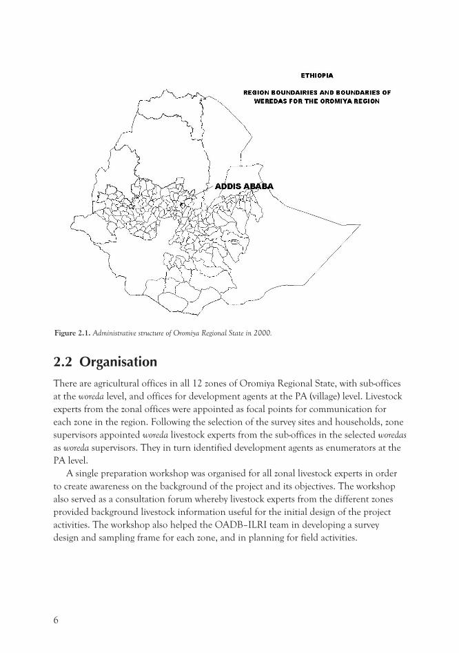
2.3 Activities
Planning is the first activity in a breed survey. The second activity is the implementation
of the planned activities. Figure 2.2 shows the activities of the breed survey along a time
line. Each of these activities lasted about eight months. Field work was followed by data
entry, which took about nine months, as well as data analysis and report writing. The
time taken by these activities was determined by the scope of the survey, the timeliness of
the field work (e.g. timing of field activities as preferred by enumerators and farmers),
resource availability (e.g. the number of computers and data-entry assistants) and the
available budget.
7
August 2001 2002 2003
Planning
Field work
Data entry
Data analysis
December 2000:
Zonal supervisors workshop
February 2003:
Reporting back workshop
April
Pre-test
Report writing
Planning
Fieldwork
Data entry
August 2001 2002 2003
Planning
Field work
Data entry
Data analysis
December 2000:
Zonal supervisors workshop
February 2003:
Reporting back workshop
April
Pre-test
Report writing
Planning
Fieldwork
Data entry
Figure 2.2. Time schedule of project activities in Oromiya Regional State.
3 Development and design of samplingframe3.1 SamplingBefore designing the livestock breed survey in Oromiya Regional State, different ap-
proaches to sampling were considered.
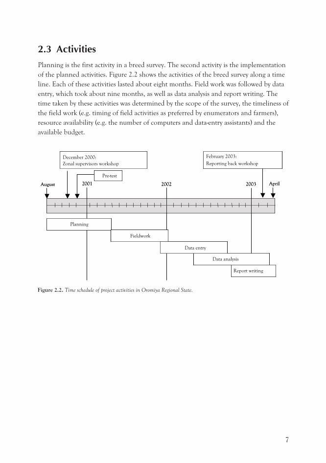
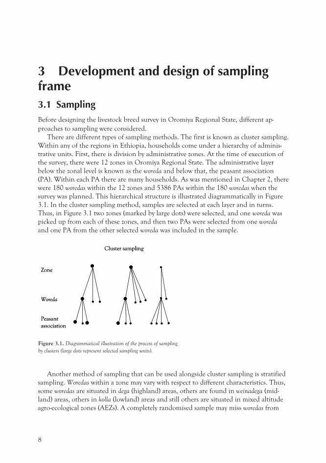
There are different types of sampling methods. The first is known as cluster sampling.
Within any of the regions in Ethiopia, households come under a hierarchy of adminis-
trative units. First, there is division by administrative zones. At the time of execution of
the survey, there were 12 zones in Oromiya Regional State. The administrative layer
below the zonal level is known as the woreda and below that, the peasant association
(PA). Within each PA there are many households. As was mentioned in Chapter 2, there
were 180 woredas within the 12 zones and 5386 PAs within the 180 woredas when the
survey was planned. This hierarchical structure is illustrated diagrammatically in Figure
3.1. In the cluster sampling method, samples are selected at each layer and in turns.
Thus, in Figure 3.1 two zones (marked by large dots) were selected, and one woreda was
picked up from each of these zones, and then two PAs were selected from one woreda
and one PA from the other selected woreda was included in the sample.
Another method of sampling that can be used alongside cluster sampling is stratified
sampling. Woredas within a zone may vary with respect to different characteristics. Thus,
some woredas are situated in dega (highland) areas, others are found in weinadega (mid-
land) areas, others in kolla (lowland) areas and still others are situated in mixed altitude
agro-ecological zones (AEZs). A completely randomised sample may miss woredas from
8
Cluster sampling
• • •
• • • • • • • • •
• •• • • • • • • •
Zone
Woreda
Peasant
association
Cluster sampling
• • •
• • • • • • • • •
• •• • • • • • • •
Zone
Woreda
Peasant
association
Figure 3.1. Diagrammatical illustration of the process of sampling
by clusters (large dots represent selected sampling units).
one of these areas. Likewise, some woredas are situated in areas of high livestock den-
sities, while others could be in areas where the livestock population is low. Grouping
woredas by AEZs and livestock densities and taking samples from each group can cover all
areas. This principle was applied in this survey, both at the zonal level, where AEZs and
livestock densities were considered, and at the woreda level where, in those woredas that
were spread over more than one AEZ, PAs were grouped by AEZ. In the survey, farming
systems were not considered for stratification purposes but it is a factor that might be
considered in future surveys, depending on the general objectives of a livestock breed
survey. A different form of stratification was considered at the PA level, namely stratifi-
cation by number of livestock in the household and whether they had cattle, sheep or
goats.
Having decided on methods to be used for stratification, alternative approaches for
sampling zones, woredas, PAs and households for the sample need to be considered.
There are essentially four methods of sampling: random, representative, convenience
and purposive. Random sampling is the only method that allows unbiased estimation of
population size. Samples are drawn completely at random, each with an equal chance of
being chosen. This method was essentially applied to select households from PAs and to
choose PAs from selected woredas. For woredas, which were themselves stratified by AEZs,
sampling was done within each stratum. When working at the PA level it may not be
easy to select households at random. An approximate method that is sometimes applied
is to define a series of trajectories and, walking along them, take every fifth household,
say, until the required number of households has been attained for each stratum. This
produces a sample that can be considered to be sufficiently random for the purposes of
the survey. For Oromiya Regional State, however, a more rigorous approach was adopted
and households were selected from a list of households compiled for the whole PA. One
disadvantage of this was that enumerators often had to travel long distances from one
household to another.
Under the representative sample approach, samples are selected in such a way that
the final selection of units is felt to be representative of the sub-population being sam-
pled. This method was applied in the selection of woredas. Whilst achieving a representa-
tive assessment of the distribution of livestock across a zone, the method, on the other
hand, makes estimation of overall number of the population in the zone more difficult.
Sometimes it may be difficult to reach a PA or certain households within a PA, and,
to make the best use of available manpower, it is more convenient to instead choose a
PA or household that is more accessible. Such a method of sampling is known as con-
venience sampling. The occasional use of this method is inevitable in such a survey, but,
provided such cases are few, it may be reasonable to assume randomness for the purpose
of estimation of number of the population.
The fourth method is purposive sampling. Under this method, sampling is based, for
example, on knowledge of a known farming system or of a breed known to be unique to
a certain area. It may not be reasonable to include such a sample for calculation of popu-
lation estimates. On the other hand, it may be important to capture information related
to the conservation of an indigenous breed. This method was sometimes applied in the
Oromiya Regional State livestock breed survey where zonal supervisors were asked to
9
provide information on any known pockets of unique breeds of livestock or special areas
that might be included.
3.2 Sampling frameAfter deciding on the general approach for selecting households to be included in the
survey a sampling frame can be drawn up. For the Oromiya Regional State it was de-
cided to sample all zones, a sample of woredas to be chosen within each zone and a
sample of PAs within each selected woreda. The sampling frame can thus be thought of
as follows:
• zone (woredas within each zone were stratified by AEZs and livestock densities)
• woreda (PAs within each woreda were stratified by AEZ) and
• PA (households within PA were stratified by number of animals they keep).
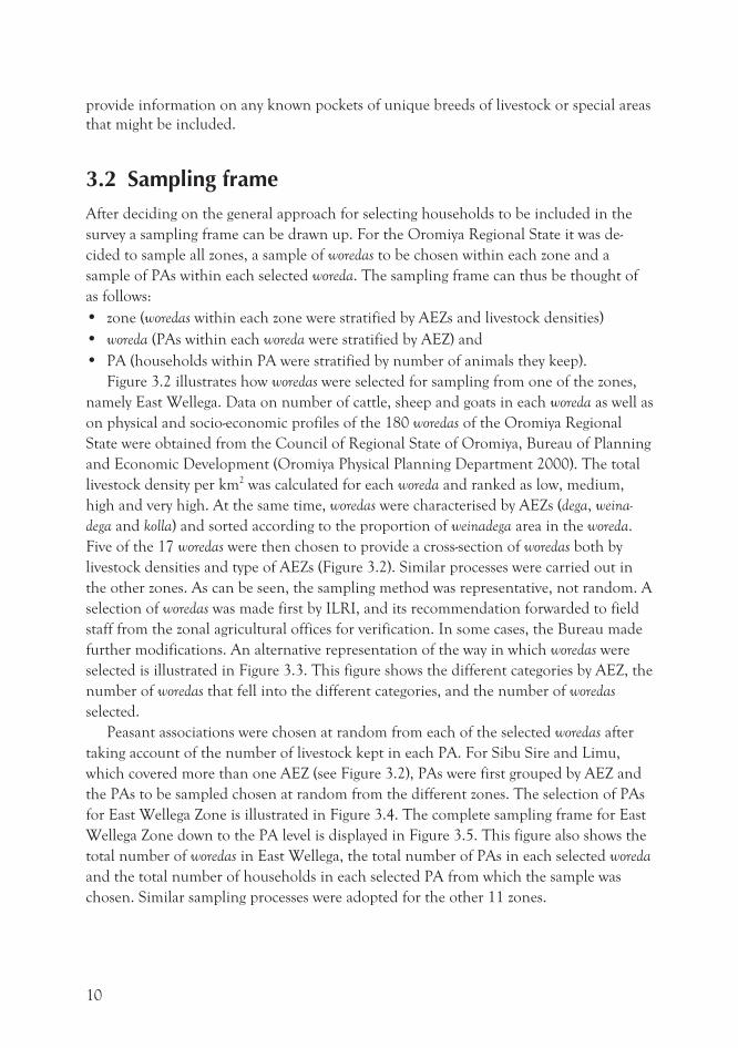
Figure 3.2 illustrates how woredas were selected for sampling from one of the zones,
namely East Wellega. Data on number of cattle, sheep and goats in each woreda as well as
on physical and socio-economic profiles of the 180 woredas of the Oromiya Regional
State were obtained from the Council of Regional State of Oromiya, Bureau of Planning
and Economic Development (Oromiya Physical Planning Department 2000). The total
livestock density per km2 was calculated for each woreda and ranked as low, medium,
high and very high. At the same time, woredas were characterised by AEZs (dega, weina-
dega and kolla) and sorted according to the proportion of weinadega area in the woreda.
Five of the 17 woredas were then chosen to provide a cross-section of woredas both by
livestock densities and type of AEZs (Figure 3.2). Similar processes were carried out in
the other zones. As can be seen, the sampling method was representative, not random. A
selection of woredas was made first by ILRI, and its recommendation forwarded to field
staff from the zonal agricultural offices for verification. In some cases, the Bureau made
further modifications. An alternative representation of the way in which woredas were
selected is illustrated in Figure 3.3. This figure shows the different categories by AEZ, the
number of woredas that fell into the different categories, and the number of woredas
selected.
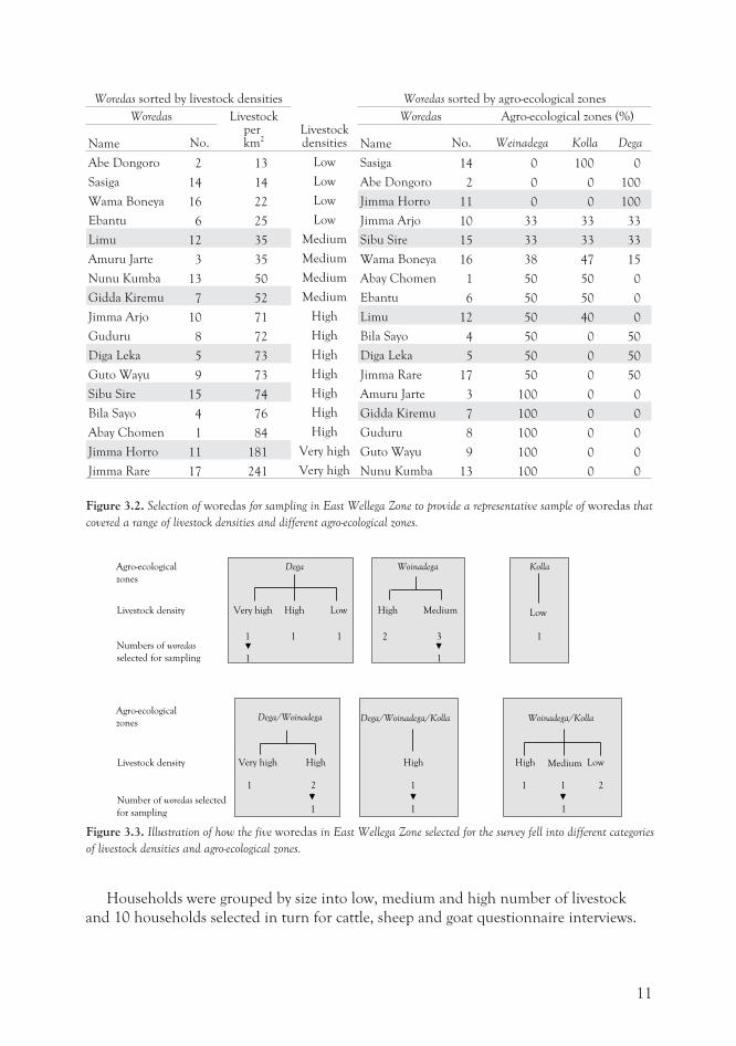
Peasant associations were chosen at random from each of the selected woredas after
taking account of the number of livestock kept in each PA. For Sibu Sire and Limu,
which covered more than one AEZ (see Figure 3.2), PAs were first grouped by AEZ and
the PAs to be sampled chosen at random from the different zones. The selection of PAs
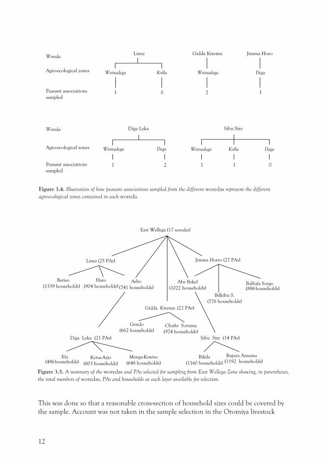
for East Wellega Zone is illustrated in Figure 3.4. The complete sampling frame for East
Wellega Zone down to the PA level is displayed in Figure 3.5. This figure also shows the
total number of woredas in East Wellega, the total number of PAs in each selected woreda
and the total number of households in each selected PA from which the sample was
chosen. Similar sampling processes were adopted for the other 11 zones.
10
Households were grouped by size into low, medium and high number of livestock
and 10 households selected in turn for cattle, sheep and goat questionnaire interviews.
11
Woredas sorted by livestock densities
Livestockdensities
Woredas sorted by agro-ecological zones
Woredas Livestockperkm2
Woredas Agro-ecological zones (%)
Name No. Name No. Weinadega Kolla Dega
Abe Dongoro 2 13 Low Sasiga 14 0 100 0
Sasiga 14 14 Low Abe Dongoro 2 0 0 100
Wama Boneya 16 22 Low Jimma Horro 11 0 0 100
Ebantu 6 25 Low Jimma Arjo 10 33 33 33
Limu 12 35 Medium Sibu Sire 15 33 33 33
Amuru Jarte 3 35 Medium Wama Boneya 16 38 47 15
Nunu Kumba 13 50 Medium Abay Chomen 1 50 50 0
Gidda Kiremu 7 52 Medium Ebantu 6 50 50 0
Jimma Arjo 10 71 High Limu 12 50 40 0
Guduru 8 72 High Bila Sayo 4 50 0 50
Diga Leka 5 73 High Diga Leka 5 50 0 50
Guto Wayu 9 73 High Jimma Rare 17 50 0 50
Sibu Sire 15 74 High Amuru Jarte 3 100 0 0
Bila Sayo 4 76 High Gidda Kiremu 7 100 0 0
Abay Chomen 1 84 High Guduru 8 100 0 0
Jimma Horro 11 181 Very high Guto Wayu 9 100 0 0
Jimma Rare 17 241 Very high Nunu Kumba 13 100 0 0
Figure 3.2. Selection of woredas for sampling in East Wellega Zone to provide a representative sample of woredas that
covered a range of livestock densities and different agro-ecological zones.
Agro-ecological
zones
Dega Woinadega Kolla
Livestock density Very high High Low MediumHigh Low
Numbers of woredas
selected for sampling
1 1 1 2 3 1
1 1
Dega/Woinadega Dega/Woinadega/Kolla Woinadega/Kolla
Livestock density Very high High LowMediumHighHigh
Number of woredas selected
for sampling
1 2 1 1 21
1 1
Agro-ecological
zones
1
Figure 3.3. Illustration of how the five woredas in East Wellega Zone selected for the survey fell into different categories
of livestock densities and agro-ecological zones.
This was done so that a reasonable cross-section of household sizes could be covered by
the sample. Account was not taken in the sample selection in the Oromiya livestock
12
Menga-Kewiso
(648 households)
East Wellega (17 woredas)
Limu (25 PAs) Jimma Horro (27 PAs)
Beriso
(1339 households)
Haro
(904 households)Abe Bekel
(1022 households)
Bilkiltu S.
(776 households)
Balbala Sorgo(886 households)
Gidda Kiremu (22 PAs)
Gendo
(662 households)Chafte Soruma
(974 households)
Diga Leka (21 PAs) Sibu Sire (14 PAs)
Efa(486households)
Kersa-Arjo
(803 households)
Bikila
(1160 households)
Bujura Amuma(1192 households)
Asbo
(741 households)
Figure 3.5. A summary of the woredas and PAs selected for sampling from East Wellega Zone showing, in parentheses,
the total numbers of woredas, PAs and households at each layer available for selection.
Woreda
Agro-ecological zones
Limu
Woinadega Kolla
3 0
Gidda Kiremu
Woinadega
2
Jimma Horo
Dega
3Peasant associations
sampled
Woreda
Agro-ecological zones
Diga Leka
Woinadega Dega
1 2Peasant associations
sampled
Sibu Sire
Woinadega Kolla Dega
1 1 0
Figure 3.4. Illustration of how peasant associations sampled from the different woredas represent the different
agro-ecological zones contained in each woreda.
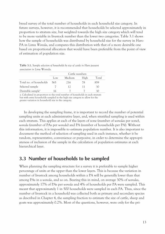
breed survey of the total number of households in each household size category. In
future surveys, however, it is recommended that households be selected approximately in
proportion to stratum size, but weighted towards the high size category which will tend
to be more variable in livestock number than the lower two categories. Table 3.1 shows
how the sample of households was distributed by household size for the survey in Haro
PA in Limu Woreda, and compares this distribution with that of a more desirable one
based on proportional allocation that would have been preferable from the point of view
of estimation of population size.
Table 3.1. Sample selection of households by size of cattle in Haro peasant
association in Limu Woreda.
Cattle numbers
Low Medium High Total
Total no. of households 565 216 78 859
Selected sample 7 12 11 30
Desirable samplea 16 7 7 30
a. Calculated in proportion to the total number of households in each stratumbut with extra households sampled in the high size category to allow for thegreater variation in household size in the category.
In developing the sampling frame, it is important to record the number of potential
sampling units at each administrative layer, and, when stratified sampling is used within
each stratum. This applies at each of the layers of zone (number of woredas per zone),
woreda (number of PAs per woreda) and PA (number of households per PA). Without
this information, it is impossible to estimate population number. It is also important to
document the method of selection of sampling used in each instance, whether it be
random, representative, convenience or purposive, in order to determine the appropri-
ateness of inclusion of the sample in the calculation of population estimates at each
hierarchical layer.
3.3 Number of households to be sampledWhen planning the sampling structure for a survey it is preferable to sample higher
percentage of units at the upper than the lower layers. This is because the variation in
number of livestock among households within a PA will be generally lower than that
among PAs in a woreda, and so on. Bearing this in mind, on average 30% of woredas,
approximately 17% of PAs per woreda and 4% of households per PA were sampled. This
meant that approximately 1 in 500 households were sampled in each PA. Thus, since the
number of livestock in a household was collected both as primary and secondary species
as described in Chapter 4, the sampling fraction to estimate the size of cattle, sheep and
goats was approximately 0.2%. Most of the questions, however, were only for the pri-
13
mary species. For these questions, the sampling fraction was reduced by a third to
0.067%.
How does one decide on how large a sample survey should be? This depends on
funds, costs of organising the survey, manpower, administrative support, means of tran-
sport and ease of access to PAs and households. It also depends on the different types of
information to be collected. If population estimation is an important objective of a sur-
vey then the sampling fraction will need to be increased somewhat towards 1%. But
5587 households were sampled in the Oromiya Regional State livestock breed survey
and this is a large number—just about the maximum that could be contemplated within
the time scale permitted. Should population estimation be an important survey requisite
then one approach could be to undertake a subsidiary survey, in parallel within the same
PAs to collect information only on livestock number.
The distribution of sampled households across PAs and woredas is illustrated in Table
5.1. Four to five woredas were selected per zone depending on the size of the zone. Be-
tween 13–25 PAs were selected per woreda. Numbers were proportional to the numbers
of PAs in each woreda. On average, 30 households were selected in each selected PA. The
cattle questionnaire was used in 10, the sheep questionnaire in 10 and the goat question-
naire in 10 of the 30 households.
14
4 Questionnaire design and contentCharacterisation of animal genetic resources (AnGR) not only involves a description of
animals, what they physically look like and what traits and production characteristics
they have, but also a description of the environment in which the animals are kept, both
the natural and production environments and the husbandry practices employed by
farmers. Therefore, the questionnaires designed for the breed survey covered aspects of
the environment as well as characterisations of the animals themselves.
4.1 QuestionnairesThree types of questionnaires were developed, each with a main focus on either cattle,
sheep or goats. These three species were referred to as ‘primary’ species. Cattle, sheep
and goats were selected as primary species owing to their high numbers and wide distri-
bution in the region under study. Within each of the three questionnaire types, infor-
mation was also collected on the other species, which were referred to as ‘secondary’
species. These were chickens, donkeys, mules, horses and camels. When cattle, sheep or
goats were not the primary species in an area, information was also collected on them as
a secondary species. This was done in order to reduce the overall size of a questionnaire
but without leaving out any of the livestock species mentioned above.
The questionnaires were designed to collect information on:
• the environment in which the animals were kept (e.g. descriptors of the environment,
farming system, husbandry practices etc.)
• breed types observed in the region
• herd/flock structure
• population size and trend
• physical, adaptive and production characteristics and
• main uses and reasons for keeping different species of livestock.
Data collected on the secondary species were less detailed. The content of the ques-
tionnaires on either primary or secondary species was as follows:
• location and identification of the interview: details of the enumerator, farmer and
location of the household
• general information of the household: number of household members, age and
gender information, size and type of land holding, numbers and types of livestock
species owned
• production systems: husbandry practices employed by farmers and purposes for
keeping livestock species, e.g. cattle, sheep or goats
15
• health aspects: diseases prevalent in the area, farmers’ opinions on disease tolerance/
resistance of their livestock, treatments (including traditional ones), types of veterin-
ary services available and distances to veterinary services
• breeding, mating and castration practices: type of mating, breeding method, sources
of breeding bulls/rams/bucks, reasons for keeping them, criteria for their choice and
castration practices
• herd dynamics: numbers of animals that entered and left the household over the
previous year, methods of sale and reasons for disposal
• breed specific information (focusing on pure breeds and crossbreds separately and
collected for both primary and secondary species): breed names, number of animals
(including gender and age), trends in composition of farmers’ livestock, reasons for
trends, origins of breeds and qualities of breed traits as assessed by farmers
• phenotypic description: coat colour of several body parts of the farmers’ animals,
description of physical appearance of the animals by qualitative and quantitative
assessment and
• production characteristics: production and reproduction.
The questionnaires consisted of open-ended, closed-ended and scaled-response
questions.
4.2 Additional survey materialsAdditional survey materials were developed and prepared to assist the enumerators
during the completion of a questionnaire. The additional survey materials consisted of:
• translated questionnaires: all three types of questionnaires were translated into
Amharic. These were not completed during our interview but one copy was given to
each enumerator to assist him/her during an interview with a farmer. This was done
to minimise possible differences in interpretation of the questions.
• descriptor list of phenotypic characteristics of animals: a descriptor list, together with
photographs of different animals, was prepared to assist with the qualitative descrip-
tion of the animals
• colour chart: developed to describe the coat colour of the animals
• measurement tape: used to measure the quantitative physical characteristics of the
animals, e.g. girth, body length.
A pre-test was conducted on the questionnaire prior to the actual survey in West and
East Shewa zones to evaluate the appropriateness of its design, clarity of the questions,
interpretation of the questions by enumerators and farmers, relevance of the questions,
quality of the data recorded, and the time taken for an interview. Results from the pre-
test were used to make a few final refinements to the questionnaires.
16
5 Field work activities5.1 Field work organisationThe Oromiya Regional State was divided into four phases to segment the field activities
of the survey. This was done to simplify the conducting of the survey, because the region
was too large to implement the survey in one phase. To avoid any coincidence of the
survey activities with rainy seasons (and their inevitable effects on road accessibility) or
with cropping activities, it was decided to divide the region into four phases on the basis
of seasons of rainfall, accessibility, crop activities and zone location (Table 5.1). The sur-
vey started in Borana Zone in May 2001 and ended in West Wellega Zone in December
2001. Between each phase, there were short intervals of one to two weeks to prepare for
the next phase, e.g. to restore supplies such as questionnaires and training material, carry
out maintenance work on vehicles etc.
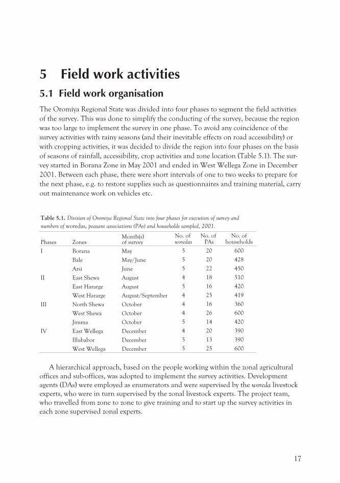
Table 5.1. Division of Oromiya Regional State into four phases for execution of survey and
numbers of woredas, peasant associations (PAs) and households sampled, 2001.
Phases ZonesMonth(s)of survey
No. ofworedas
No. ofPAs
No. ofhouseholds
I Borana May 5 20 600
Bale May/June 5 20 428
Arsi June 5 22 450
II East Shewa August 4 18 510
East Hararge August 5 16 420
West Hararge August/September 4 25 419
III North Shewa October 4 16 360
West Shewa October 4 26 600
Jimma October 5 14 420
IV East Wellega December 4 20 390
Illubabor December 5 13 390
West Wellega December 5 25 600
A hierarchical approach, based on the people working within the zonal agricultural
offices and sub-offices, was adopted to implement the survey activities. Development
agents (DAs) were employed as enumerators and were supervised by the woreda livestock
experts, who were in turn supervised by the zonal livestock experts. The project team,
who travelled from zone to zone to give training and to start up the survey activities in
each zone supervised zonal experts.
17
5.2 Enumerator and supervisor trainingTraining content, method and duration are important aspects to be considered when
preparing for training. A suitably long and well-conducted course helps to ensure good
quality of data collected later during the livestock breed survey. Both supervisors and
enumerators attended the training courses. Training was given to enumerators and
supervisors in each zone prior to the commencement of the survey in the zone. Each
training period took three days, and contained classroom training and group exercises
on the first and second days, and field exercises on the third day. The training covered
the background and the objectives of the project, careful examination of each question
in the questionnaires, and interviewing techniques. During the course of the training
ample time was allocated for discussions and practices.
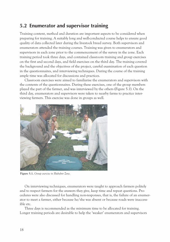
Classroom exercises were aimed to familiarise the enumerators and supervisors with
the contents of the questionnaires. During these exercises, one of the group members
played the part of the farmer, and was interviewed by the others (Figure 5.1). On the
third day, enumerators and supervisors were taken to nearby farms to practice inter-
viewing farmers. This exercise was done in groups as well.
On interviewing techniques, enumerators were taught to approach farmers politely
and to respect farmers for the answers they give, keep time and repeat questions. Pro-
cedures were also discussed for handling non-responses, that is, the failure of an enumer-
ator to meet a farmer, either because he/she was absent or because roads were inaccess-
ible etc.
Three days is recommended as the minimum time to be allocated for training.
Longer training periods are desirable to help the ‘weaker’ enumerators and supervisors
18
Figure 5.1. Group exercise in Illubabor Zone.
to get a better understanding of the questionnaires. A longer course also allows for
greater individual tuition.
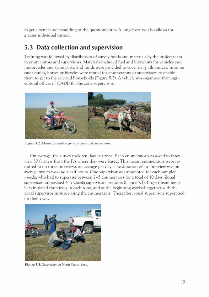
5.3 Data collection and supervisionTraining was followed by distribution of survey funds and materials by the project team
to enumerators and supervisors. Materials included fuel and lubricants for vehicles and
motorcycles and spare parts, and funds were provided to cover daily allowances. In some
cases mules, horses or bicycles were rented for enumerators or supervisors to enable
them to get to the selected households (Figure 5.2). A vehicle was organised from agri-
cultural offices of OADB for the zone supervisors.
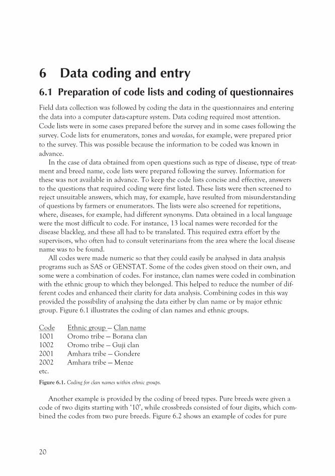
On average, the survey took ten days per zone. Each enumerator was asked to inter-
view 30 farmers from the PA where they were based. This meant enumerators were re-
quired to do three interviews on average per day. The duration of an interview was on
average two to two-and-a-half hours. One supervisor was appointed for each sampled
woreda, who had to supervise between 2–5 enumerators for a total of 10 days. Zonal
supervisors supervised 4–5 woreda supervisors per zone (Figure 5.3). Project team mem-
bers initiated the survey in each zone, and at the beginning worked together with the
zonal supervisor in supervising the enumerators. Thereafter, zonal supervisors supervised
on their own.
19
Figure 5.3. Supervision in North Shewa Zone.
Figure 5.2. Means of transport for supervisors and enumerators.
6 Data coding and entry6.1 Preparation of code lists and coding of questionnairesField data collection was followed by coding the data in the questionnaires and entering
the data into a computer data-capture system. Data coding required most attention.
Code lists were in some cases prepared before the survey and in some cases following the
survey. Code lists for enumerators, zones and woredas, for example, were prepared prior
to the survey. This was possible because the information to be coded was known in
advance.
In the case of data obtained from open questions such as type of disease, type of treat-
ment and breed name, code lists were prepared following the survey. Information for
these was not available in advance. To keep the code lists concise and effective, answers
to the questions that required coding were first listed. These lists were then screened to
reject unsuitable answers, which may, for example, have resulted from misunderstanding
of questions by farmers or enumerators. The lists were also screened for repetitions,
where, diseases, for example, had different synonyms. Data obtained in a local language
were the most difficult to code. For instance, 13 local names were recorded for the
disease blackleg, and these all had to be translated. This required extra effort by the
supervisors, who often had to consult veterinarians from the area where the local disease
name was to be found.
All codes were made numeric so that they could easily be analysed in data analysis
programs such as SAS or GENSTAT. Some of the codes given stood on their own, and
some were a combination of codes. For instance, clan names were coded in combination
with the ethnic group to which they belonged. This helped to reduce the number of dif-
ferent codes and enhanced their clarity for data analysis. Combining codes in this way
provided the possibility of analysing the data either by clan name or by major ethnic
group. Figure 6.1 illustrates the coding of clan names and ethnic groups.
Code Ethnic group — Clan name
1001 Oromo tribe — Borana clan
1002 Oromo tribe — Guji clan
2001 Amhara tribe — Gondere
2002 Amhara tribe — Menze
etc.
Figure 6.1. Coding for clan names within ethnic groups.
Another example is provided by the coding of breed types. Pure breeds were given a
code of two digits starting with ‘10’, while crossbreds consisted of four digits, which com-
bined the codes from two pure breeds. Figure 6.2 shows an example of codes for pure
20
breeds and crossbreds. Codes for woreda, PA and household formed together a unique
code that distinguished one questionnaire from another. One member of the project
team did coding of questionnaires to ensure that the answers were interpreted consist-
ently.
Code Pure breeds and crossbreds
10 Arsi
11 Borana
13 Guji
1011 Arsi × Borana crossa
1113 Borana × Guji cross
etc.
a. The two pure breed codes to form the crossbred code were combined by having the lower number appear first.
Figure 6.2. Coding for pure breed and crossbred types.
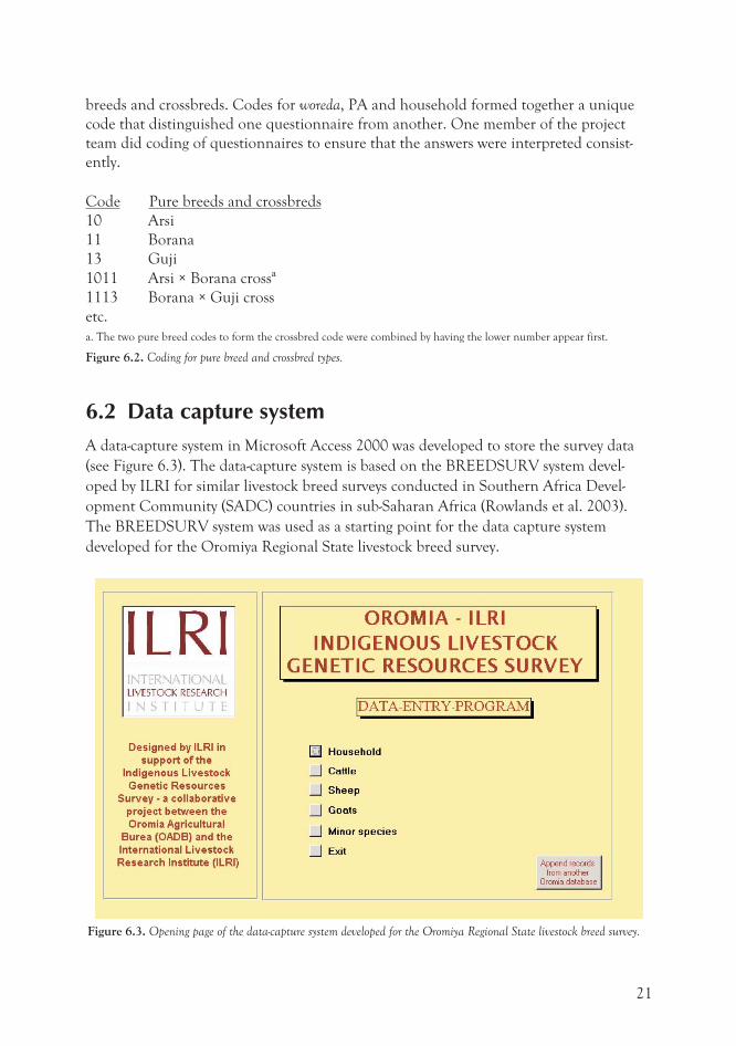
6.2 Data capture systemA data-capture system in Microsoft Access 2000 was developed to store the survey data
(see Figure 6.3). The data-capture system is based on the BREEDSURV system devel-
oped by ILRI for similar livestock breed surveys conducted in Southern Africa Devel-
opment Community (SADC) countries in sub-Saharan Africa (Rowlands et al. 2003).
The BREEDSURV system was used as a starting point for the data capture system
developed for the Oromiya Regional State livestock breed survey.
21
Figure 6.3. Opening page of the data-capture system developed for the Oromiya Regional State livestock breed survey.
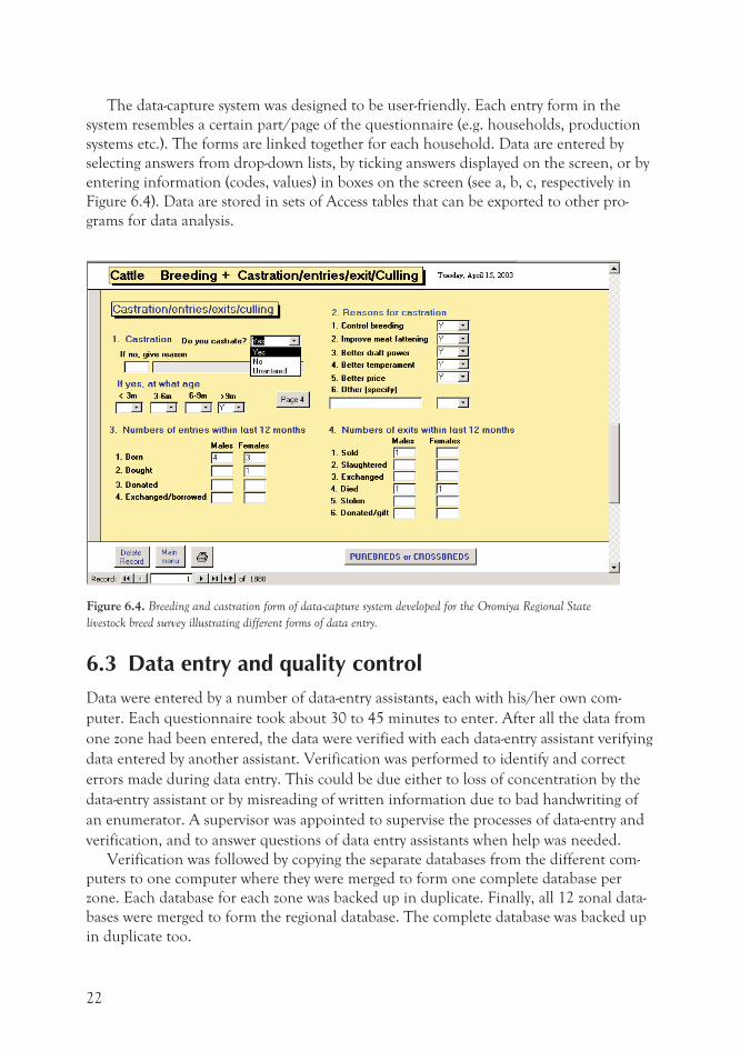
The data-capture system was designed to be user-friendly. Each entry form in the
system resembles a certain part/page of the questionnaire (e.g. households, production
systems etc.). The forms are linked together for each household. Data are entered by
selecting answers from drop-down lists, by ticking answers displayed on the screen, or by
entering information (codes, values) in boxes on the screen (see a, b, c, respectively in
Figure 6.4). Data are stored in sets of Access tables that can be exported to other pro-
grams for data analysis.
6.3 Data entry and quality controlData were entered by a number of data-entry assistants, each with his/her own com-
puter. Each questionnaire took about 30 to 45 minutes to enter. After all the data from
one zone had been entered, the data were verified with each data-entry assistant verifying
data entered by another assistant. Verification was performed to identify and correct
errors made during data entry. This could be due either to loss of concentration by the
data-entry assistant or by misreading of written information due to bad handwriting of
an enumerator. A supervisor was appointed to supervise the processes of data-entry and
verification, and to answer questions of data entry assistants when help was needed.
Verification was followed by copying the separate databases from the different com-
puters to one computer where they were merged to form one complete database per
zone. Each database for each zone was backed up in duplicate. Finally, all 12 zonal data-
bases were merged to form the regional database. The complete database was backed up
in duplicate too.
22
Figure 6.4. Breeding and castration form of data-capture system developed for the Oromiya Regional State
livestock breed survey illustrating different forms of data entry.
7 Survey budget7.1 Budget preparationCareful budget preparation is important in the planning of a livestock breed survey. The
budget for the Oromiya Regional State livestock breed survey was prepared in advance of
the initiation of the project, which meant that many of the planning issues were resolved
before the survey began. Overall, the budget prepared for the survey was meant to cover
expenses for three components:
1. planning
• preliminary meeting
• setting up general administrative organisation
• planning and preparation of survey design
• pre-surveys—listing of households in villages to be sampled
• preparation of survey materials
• pilot surveys—pre-testing of questionnaires
2. executing survey activities
• training
• survey
3. data processing
• data management, data coding, entry and verification
• data analysis and report writing
• reporting back meeting.
The size of budget for a survey depends on:
• the size of the sample, number of sampled households
• number of enumerators and supervisors involved
• means of transport to be used by supervisors and enumerators
• fuel and lubricants requirements
• number of computers available and number of data-entry assistants required
• number of people involved in data analysis and report writing.
7.2 ExpensesThe expenses provided during the execution of the survey activities needed most atten-
tion. This was due to the differences in expenses required by each zone. Some zones had
sufficient means of transport, while others had not. The larger zones tended to require
more fuel and lubricants for transport than the smaller zones. Figure 7.1 shows the
23
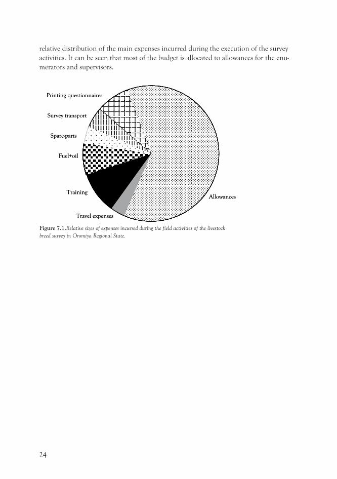
relative distribution of the main expenses incurred during the execution of the survey
activities. It can be seen that most of the budget is allocated to allowances for the enu-
merators and supervisors.
24
AllowancesTraining
Travel expenses
Fuel+oil
Spare-parts
Survey transport
Printing questionnaires
AllowancesTraining
Travel expenses
Fuel+oil
Spare-parts
Survey transport
Printing questionnaires
Figure 7.1.Relative sizes of expenses incurred during the field activities of the livestock
breed survey in Oromiya Regional State.
8 Population estimationPopulation estimates are not provided in this report, as more analyses are needed to
generate this information. Here, however, a simple example is given to illustrate the
process. Generally, one might be interested in estimating the number of cattle in a PA,
in a woreda or in a zone. Since woredas were not selected randomly from zones, it will be
more difficult, as mentioned earlier, to obtain reliable population estimates at this layer.
At the PA level, however, it is easier.
8.1 Random sample of households in a PASuppose, for example, n households are sampled at random from N households in a PA.
To get an estimate of the average number of cattle per household in the sample, add the
number of cattle in the sampled households and divide by the size of the sample, n.
Write the sample mean as m.
Multiply m by n and get an estimate of the total number of cattle in PA = Nm. We
also need to calculate a standard error (se) for this estimate in order to provide some
measure of precision.
The formula for the se is:
N N n S n( ) /−
where S = Sum (y – m)2/(n – 1), where the summation is over all households, and where y
is the number of livestock in each sample household.
We can then write the estimated number of cattle in the PA as:
Nm N N n S n± −( ) /
8.2 Stratified random sample in a PAIn the case of a stratified random sample, the method gets more complicated but the
principle is the same. For example, the estimated number of cattle in a PA stratified by
household size is:
SUM Nm SUM N N n S n± −( ) /
where the individual expressions in the above formula are calculated for each stratum
and then summed. The process is illustrated for Haro PA in Limu Woreda in Table 8.1
25
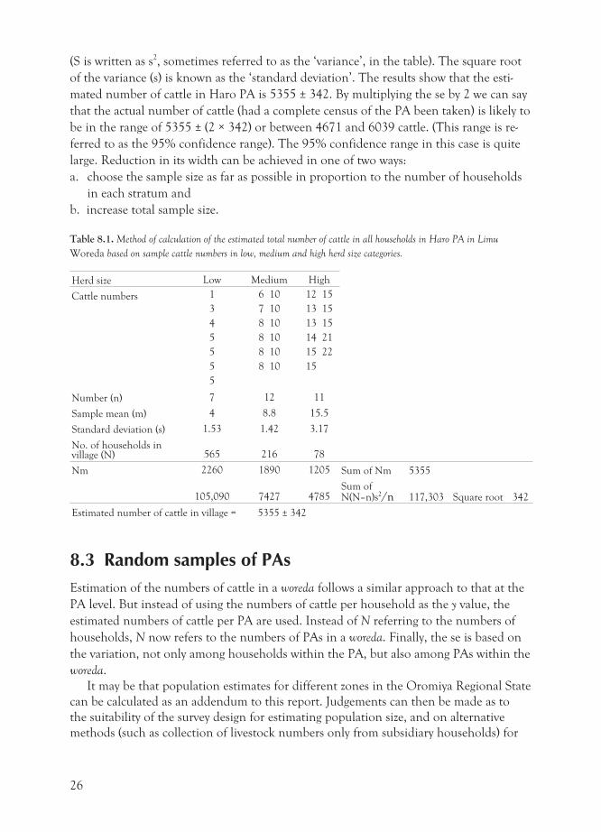
(S is written as s2, sometimes referred to as the ‘variance’, in the table). The square root
of the variance (s) is known as the ‘standard deviation’. The results show that the esti-
mated number of cattle in Haro PA is 5355 ± 342. By multiplying the se by 2 we can say
that the actual number of cattle (had a complete census of the PA been taken) is likely to
be in the range of 5355 ± (2 × 342) or between 4671 and 6039 cattle. (This range is re-
ferred to as the 95% confidence range). The 95% confidence range in this case is quite
large. Reduction in its width can be achieved in one of two ways:
a. choose the sample size as far as possible in proportion to the number of households
in each stratum and
b. increase total sample size.
Table 8.1. Method of calculation of the estimated total number of cattle in all households in Haro PA in Limu
Woreda based on sample cattle numbers in low, medium and high herd size categories.
Herd size Low Medium High
Cattle numbers
Number (n)
1 6 10 12 15
3 7 10 13 15
4 8 10 13 15
5 8 10 14 21
5 8 10 15 22
5 8 10 15
5
7 12 11
Sample mean (m) 4 8.8 15.5
Standard deviation (s) 1.53 1.42 3.17
No. of households invillage (N) 565 216 78
Nm 2260 1890 1205 Sum of Nm 5355
105,090 7427 4785Sum ofN(N–n)s2/n 117,303 Square root 342
Estimated number of cattle in village = 5355 ± 342
8.3 Random samples of PAsEstimation of the numbers of cattle in a woreda follows a similar approach to that at the
PA level. But instead of using the numbers of cattle per household as the y value, the
estimated numbers of cattle per PA are used. Instead of N referring to the numbers of
households, N now refers to the numbers of PAs in a woreda. Finally, the se is based on
the variation, not only among households within the PA, but also among PAs within the
woreda.
It may be that population estimates for different zones in the Oromiya Regional State
can be calculated as an addendum to this report. Judgements can then be made as to
the suitability of the survey design for estimating population size, and on alternative
methods (such as collection of livestock numbers only from subsidiary households) for
26

improving the precision of sample estimates. Further discussion on estimation of popu-
lation size is given in Rowlands et al. (2003) in relation to the implementation of a live-
stock breed survey in Zimbabwe.
27
9 Descriptive results9.1 Structure of data
This chapter provides a range of tables of research results. As mentioned in the previous
chapter it is not possible at present, because of the difficulties in identifying breed types
from the information provided by farmers, to provide results on a breed basis. Following
further exploratory analysis with the cluster analysis methodology in different zones,
classification of certain of the tables by breed type can be attempted at a later stage.
As mentioned earlier, AEZs and livestock densities were the two criteria used for
stratification purposes in planning the sampling frame. Three AEZs, namely: dega (high-
land), weinadega (midland) and kolla (lowland) were used, and livestock densities were
grouped into four categories: low (1–50 animals per km2), medium (51–100 animals per
km2), high (101–200 animals per km2) and very high (above 200 animals per km2).
Animal, in this case, refers to the sum of numbers of cattle, sheep and goats at the woreda
level. Many of the tables are presented, throughout this report, in turn by AEZs, live-
stock densities and the production systems. Although production systems were not used
as stratification criteria during sampling design, they were considered as important man-
agement/environmental characteristic, and so output tables are classified by production
systems too.
Wherever appropriate, the numbers of households providing data are included in
each table. Whenever the data analysed are based on single responses to questions the
percentage values should add up to 100%. Some questions, however, allow multiple
answers. In these cases, percentages will not add up to 100%. Percentage units (%) are
shown alongside the levels of one of the classification variables, either along the top or
down the side, to indicate how the contents of the tables are to be interpreted and in
which direction the percentage values are to be summed.
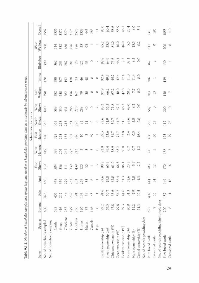
Table 9.1.1 shows the number of households interviewed during the survey through-
out the 12 zones. A total of 5587 households were sampled, on average 466 households
per zone. In addition, the table shows a breakdown of the different species of livestock
owned by the sample households. This ranged from 95% with cattle to 5% with camels
to 0.2% with pigs.
28
29
Tab
le9.1
.1.
Num
ber
ofhou
sehol
dssa
mpl
edand
spec
ies
kept
and
num
ber
ofhou
sehol
dspr
ovid
ing
data
onca
ttle
bree
dsby
adm
inis
trati
vezo
nes
.
Item
s
Ad
min
istr
ativ
ezo
nes
Sp
ecie
sB
ora
na
Bal
eA
rsi
Eas
tS
hew
aW
est
Har
arge
Eas
tH
arar
geN
ort
hS
hew
aW
est
Sh
ewa
Eas
tW
elle
gaJi
mm
aIl
lub
abo
rW
est
Wel
lega
Ove
rall
No
.o
fh
ou
seh
old
ssa
mp
led
600
428
450
510
419
420
360
600
390
420
390
600
5587
No
.o
fh
ou
seh
old
skee
pin
g
Cat
tle
595
405
448
504
389
375
355
589
382
388
362
514
5306
Sh
eep
416
217
359
336
207
225
223
339
258
207
253
332
3372
Ch
icken
s287
144
279
311
247
133
215
431
262
192
287
486
3274
Go
ats
479
232
263
339
273
301
161
286
156
178
181
276
3125
Do
nkey
s236
191
231
439
213
226
220
278
167
73
28
276
2578
Ho
rses
120
134
259
120
310
92
288
79
46
125
33
1309
Mu
les
67
34
35
30
32
21
49
30
48
33
93
445
Cam
els
146
45
611
569
00
00
01
283
Pig
s0
11
30
10
20
02
111
Cat
tle
ow
ner
ship
(%)
99.2
94.6
99.6
98.8
92.8
89.3
98.6
98.2
97.9
92.4
92.8
85.7
95.0
Sh
eep
ow
ner
ship
(%)
69.3
50.7
79.8
65.9
49.4
53.6
61.9
56.5
66.2
49.3
64.9
55.3
60.4
Ch
icken
ow
ner
ship
(%)
47.8
33.6
62.0
61.0
58.9
31.7
59.7
71.8
67.2
45.7
73.6
81.0
58.6
Go
ato
wn
ersh
ip(%
)79.8
54.2
58.4
66.5
65.2
71.7
44.7
47.7
40.0
42.4
46.4
46.0
55.9
Do
nkey
ow
ner
ship
(%)
39.3
44.6
51.3
86.1
50.8
53.8
61.1
46.3
42.8
17.4
7.2
46.0
46.1
Ho
rse
ow
ner
ship
(%)
20.0
31.3
57.6
23.5
0.7
2.4
25.6
48.0
20.3
11.0
32.1
5.5
23.4
Mu
leo
wn
ersh
ip(%
)11.2
7.9
7.8
5.9
0.7
0.5
5.8
8.2
7.7
11.4
8.5
15.5
8.0
Cam
elo
wn
ersh
ip(%
)24.3
10.5
1.3
2.2
1.2
16.4
0.0
0.0
0.0
0.0
0.0
0.2
5.1
No
.o
fre
cord
sp
rovi
din
gd
ata
Pu
reb
reed
catt
le595
402
444
503
390
400
350
587
383
386
362
511
5313
Cro
ssb
red
catt
le7
16
34
12
550
55
013
12
0195
No
.o
fre
cord
sp
rovi
din
gp
hen
oty
pic
dat
a
Pu
reb
reed
catt
le200
157
149
170
138
125
117
200
130
139
130
200
1855
Cro
ssb
red
catt
le6
11
16
65
29
28
07
11
0110
9.2 Ownership and use of land and livestock species
9.2.1 Distribution of households sampled across differentadministrative zones
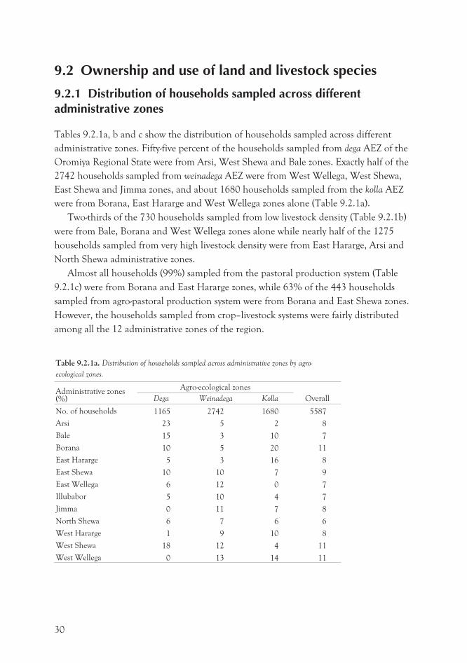
Tables 9.2.1a, b and c show the distribution of households sampled across different
administrative zones. Fifty-five percent of the households sampled from dega AEZ of the
Oromiya Regional State were from Arsi, West Shewa and Bale zones. Exactly half of the
2742 households sampled from weinadega AEZ were from West Wellega, West Shewa,
East Shewa and Jimma zones, and about 1680 households sampled from the kolla AEZ
were from Borana, East Hararge and West Wellega zones alone (Table 9.2.1a).
Two-thirds of the 730 households sampled from low livestock density (Table 9.2.1b)
were from Bale, Borana and West Wellega zones alone while nearly half of the 1275
households sampled from very high livestock density were from East Hararge, Arsi and
North Shewa administrative zones.
Almost all households (99%) sampled from the pastoral production system (Table
9.2.1c) were from Borana and East Hararge zones, while 63% of the 443 households
sampled from agro-pastoral production system were from Borana and East Shewa zones.
However, the households sampled from crop–livestock systems were fairly distributed
among all the 12 administrative zones of the region.
Table 9.2.1a. Distribution of households sampled across administrative zones by agro-
ecological zones.
Administrative zones(%)
Agro-ecological zones
OverallDega Weinadega Kolla
No. of households 1165 2742 1680 5587
Arsi 23 5 2 8
Bale 15 3 10 7
Borana 10 5 20 11
East Hararge 5 3 16 8
East Shewa 10 10 7 9
East Wellega 6 12 0 7
Illubabor 5 10 4 7
Jimma 0 11 7 8
North Shewa 6 7 6 6
West Hararge 1 9 10 8
West Shewa 18 12 4 11
West Wellega 0 13 14 11
30
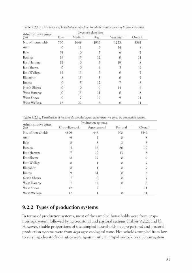
Table 9.2.1b. Distribution of households sampled across administrative zones by livestock densities.
Administrative zones(%)
Livestock densities
OverallLow Medium High Very high
No. of households 730 1649 1933 1275 5587
Arsi 0 11 5 14 8
Bale 34 0 5 6 7
Borana 16 15 12 0 11
East Hararge 12 0 5 19 8
East Shewa 0 0 6 3 9
East Wellega 12 13 5 0 7
Illubabor 8 15 5 0 7
Jimma 0 5 12 7 8
North Shewa 0 0 9 14 6
West Hararge 0 13 11 0 8
West Shewa 0 7 19 9 11
West Wellega 16 22 6 0 11
Table 9.2.1c. Distribution of households sampled across administrative zones by production systems.
Administrative zones(%)
Production systems
OverallCrop–livestock Agro-pastoral Pastoral
No. of households 4899 443 200 5542
Arsi 9 2 0 8
Bale 8 8 2 8
Borana 5 36 86 10
East Hararge 7 10 13 8
East Shewa 8 27 0 9
East Wellega 8 1 0 7
Illubabor 8 1 0 7
Jimma 9 <1 0 8
North Shewa 7 0 0 7
West Hararge 7 12 0 8
West Shewa 12 2 1 11
West Wellega 12 1 0 11
9.2.2 Types of production systems
In terms of production systems, most of the sampled households were from crop–
livestock system followed by agro-pastoral and pastoral systems (Tables 9.2.2a and b).
However, sizable proportions of the sampled households in agro-pastoral and pastoral
production systems were from dega agro-ecological zone. Households sampled from low
to very high livestock densities were again mostly in crop–livestock production system
31
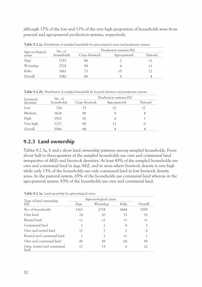
although 17% of the low and 11% of the very high proportion of households were from
pastoral and agro-pastoral production systems, respectively.
Table 9.2.2a. Distribution of sampled households by agro-ecological zones and production systems.
Agro-ecologicalzones
No. ofhouseholds
Production systems (%)
Crop–livestock Agro-pastoral Pastoral
Dega 1153 98 2 <1
Weinadega 2728 94 6 <1
Kolla 1661 73 15 12
Overall 5542 88 8 4
Table 9.2.2b. Distribution of sampled households by livestock densities and production systems.
Livestockdensities
No. ofhouseholds
Production systems (%)
Crop–livestock Agro-pastoral Pastoral
Low 728 73 10 17
Medium 1624 88 8 4
High 1925 92 6 1
Very high 1271 89 11 0
Overall 5566 88 8 4
9.2.3 Land ownership
Tables 9.2.3a, b and c show land ownership patterns among sampled households. From
about half to three-quarters of the sampled households use own and communal land
irrespective of AEZs and livestock densities. At least 45% of the sampled households use
own and communal land in dega AEZ, and in areas where livestock density is very high
while only 13% of the households use only communal land in low livestock density
areas. In the pastoral system, 65% of the households use communal land whereas in the
agro-pastoral system, 83% of the households use own and communal land.
Table 9.2.3a. Land ownership by agro-ecological zones.
Type of land ownership(%)
Agro-ecological zones
OverallDega Weinadega Kolla
No. of households 1161 2734 1664 5559
Own land 24 20 15 19
Rented land <1 <1 <1 <1
Communal land 1 1 9 3
Own and rented land 12 7 2 6
Rented and communal land 1 1 <1 1
Own and communal land 45 58 68 59
Own, rented and communalland
17 13 6 12
32
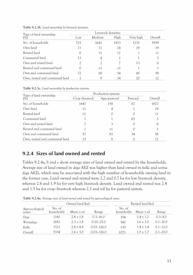
Table 9.2.3b. Land ownership by livestock densities.
Type of land ownership(%)
Livestock densities
OverallLow Medium High Very high
No. of households 725 1641 1923 1270 5559
Own land 11 17 24 19 19
Rented land 0 <1 <1 1 <1
Communal land 13 4 1 1 3
Own and rented land 2 2 7 13 6
Rented and communal land 0 <1 <1 1 1
Own and communal land 72 68 54 45 59
Own, rented and communal land 1 9 14 20 12
Table 9.2.3c. Land ownership by production systems.
Type of land ownership(%)
Production systems
OverallCrop–livestock Agro-pastoral Pastoral
No. of households 1647 158 67 1872
Own land 21 4 1 19
Rented land <1 0 0 <1
Communal land 1 1 65 3
Own and rented land 7 3 0 6
Rented and communal land 1 <1 0 1
Own and communal land 57 83 34 58
Own, rented and communal land 13 8 0 12
9.2.4 Sizes of land owned and rented
Tables 9.2.4a, b and c show average sizes of land owned and rented by the households.
Average size of land owned in dega AEZ was higher than land owned in kolla and weina-
dega AEZs, which may be associated with the high number of households owning land in
the former case. Land owned and rented were 2.2 and 0.7 ha for low livestock density,
whereas 2.6 and 1.9 ha for very high livestock density. Land owned and rented was 2.4
and 1.5 ha for crop–livestock whereas 2.1 and nil ha for pastoral system.
Table 9.2.4a. Average sizes of land owned and rented by agro-ecological zones.
Agro-ecologicalzones
Owned land (ha) Rented land (ha)
No. ofhouseholds Mean ± sd Range
No. ofhouseholds Mean ± sd Range
Dega 1141 2.8 ± 1.8 0.3–16.0 354 1.4 ± 1.2 0.3–8.0
Weinadega 2682 2.3 ± 1.8 0.10–25.0 580 1.6 ± 2.0 0.1–20.0
Kolla 1511 2.4 ± 4.9 0.03–126.0 139 1.4 ± 1.4 0.1–12.0
Overall 5334 2.4 ± 3.0 0.03–126.0 1073 1.5 ± 1.7 0.1–20.0
33
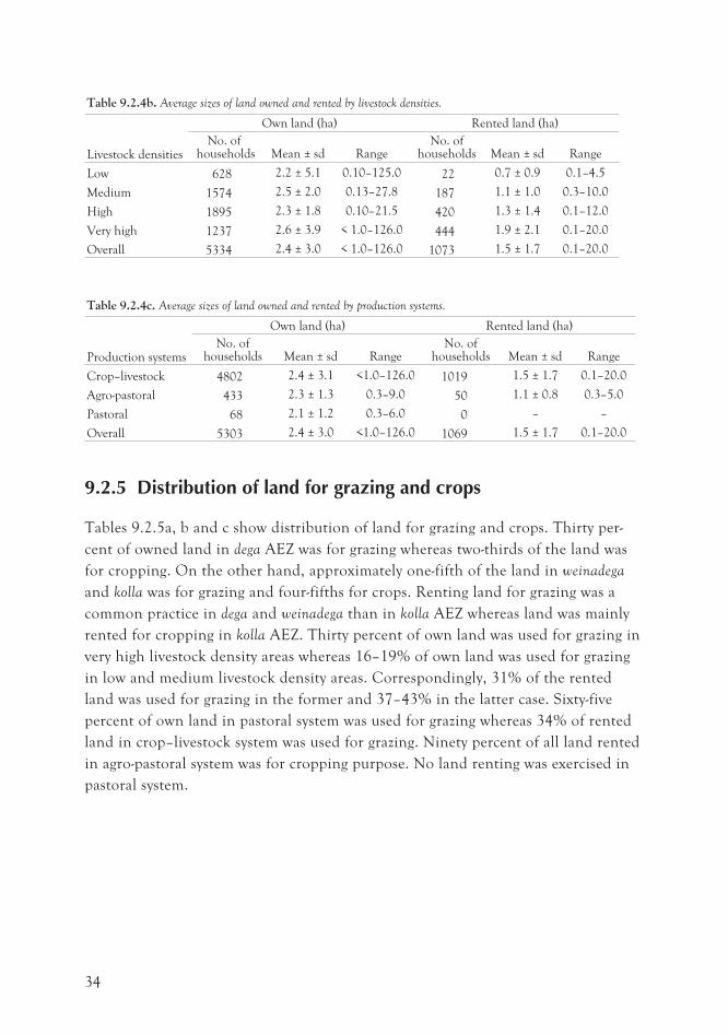
Table 9.2.4b. Average sizes of land owned and rented by livestock densities.
Livestock densities
Own land (ha) Rented land (ha)
No. ofhouseholds Mean ± sd Range
No. ofhouseholds Mean ± sd Range
Low 628 2.2 ± 5.1 0.10–125.0 22 0.7 ± 0.9 0.1–4.5
Medium 1574 2.5 ± 2.0 0.13–27.8 187 1.1 ± 1.0 0.3–10.0
High 1895 2.3 ± 1.8 0.10–21.5 420 1.3 ± 1.4 0.1–12.0
Very high 1237 2.6 ± 3.9 < 1.0–126.0 444 1.9 ± 2.1 0.1–20.0
Overall 5334 2.4 ± 3.0 < 1.0–126.0 1073 1.5 ± 1.7 0.1–20.0
Table 9.2.4c. Average sizes of land owned and rented by production systems.
Production systems
Own land (ha) Rented land (ha)
No. ofhouseholds Mean ± sd Range
No. ofhouseholds Mean ± sd Range
Crop–livestock 4802 2.4 ± 3.1 <1.0–126.0 1019 1.5 ± 1.7 0.1–20.0
Agro-pastoral 433 2.3 ± 1.3 0.3–9.0 50 1.1 ± 0.8 0.3–5.0
Pastoral 68 2.1 ± 1.2 0.3–6.0 0 – –
Overall 5303 2.4 ± 3.0 <1.0–126.0 1069 1.5 ± 1.7 0.1–20.0
9.2.5 Distribution of land for grazing and crops
Tables 9.2.5a, b and c show distribution of land for grazing and crops. Thirty per-
cent of owned land in dega AEZ was for grazing whereas two-thirds of the land was
for cropping. On the other hand, approximately one-fifth of the land in weinadega
and kolla was for grazing and four-fifths for crops. Renting land for grazing was a
common practice in dega and weinadega than in kolla AEZ whereas land was mainly
rented for cropping in kolla AEZ. Thirty percent of own land was used for grazing in
very high livestock density areas whereas 16–19% of own land was used for grazing
in low and medium livestock density areas. Correspondingly, 31% of the rented
land was used for grazing in the former and 37–43% in the latter case. Sixty-five
percent of own land in pastoral system was used for grazing whereas 34% of rented
land in crop–livestock system was used for grazing. Ninety percent of all land rented
in agro-pastoral system was for cropping purpose. No land renting was exercised in
pastoral system.
34
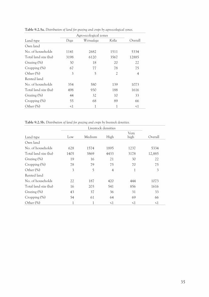
Table 9.2.5a. Distribution of land for grazing and crops by agro-ecological zones.
Land type
Agro-ecological zones
OverallDega Weinadega Kolla
Own land
No. of households 1141 2682 1511 5334
Total land size (ha) 3198 6120 3567 12885
Grazing (%) 30 18 20 22
Cropping (%) 67 77 78 75
Other (%) 3 5 2 4
Rented land
No. of households 354 580 139 1073
Total land size (ha) 498 930 188 1616
Grazing (%) 44 32 10 33
Cropping (%) 55 68 89 66
Other (%) <1 1 1 <1
Table 9.2.5b. Distribution of land for grazing and crops by livestock densities.
Land type
Livestock densities
OverallLow Medium HighVeryhigh
Own land
No. of households 628 1574 1895 1237 5334
Total land size (ha) 1405 3869 4433 3178 12,885
Grazing (%) 19 16 21 30 22
Cropping (%) 78 79 75 70 75
Other (%) 3 5 4 1 3
Rented land
No. of households 22 187 420 444 1073
Total land size (ha) 16 203 541 856 1616
Grazing (%) 43 37 36 31 33
Cropping (%) 54 61 64 69 66
Other (%) 1 1 <1 <1 <1
35
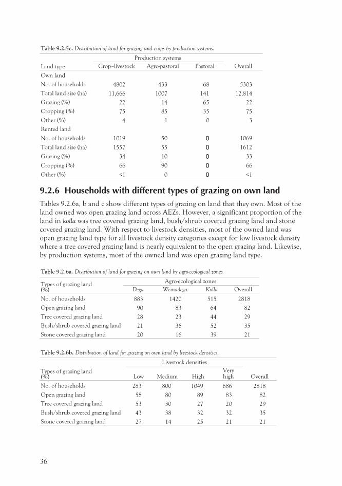
Table 9.2.5c. Distribution of land for grazing and crops by production systems.
Land type
Production systems
OverallCrop–livestock Agro-pastoral Pastoral
Own land
No. of households 4802 433 68 5303
Total land size (ha) 11,666 1007 141 12,814
Grazing (%) 22 14 65 22
Cropping (%) 75 85 35 75
Other (%) 4 1 0 3
Rented land
No. of households 1019 50 0 1069
Total land size (ha) 1557 55 0 1612
Grazing (%) 34 10 0 33
Cropping (%) 66 90 0 66
Other (%) <1 0 0 <1
9.2.6 Households with different types of grazing on own landTables 9.2.6a, b and c show different types of grazing on land that they own. Most of theland owned was open grazing land across AEZs. However, a significant proportion of theland in kolla was tree covered grazing land, bush/shrub covered grazing land and stonecovered grazing land. With respect to livestock densities, most of the owned land wasopen grazing land type for all livestock density categories except for low livestock densitywhere a tree covered grazing land is nearly equivalent to the open grazing land. Likewise,by production systems, most of the owned land was open grazing land type.
Table 9.2.6a. Distribution of land for grazing on own land by agro-ecological zones.
Types of grazing land(%)
Agro-ecological zones
Dega Weinadega Kolla Overall
No. of households 883 1420 515 2818
Open grazing land 90 83 64 82
Tree covered grazing land 28 23 44 29
Bush/shrub covered grazing land 21 36 52 35
Stone covered grazing land 20 16 39 21
Table 9.2.6b. Distribution of land for grazing on own land by livestock densities.
Types of grazing land(%)
Livestock densities
OverallLow Medium HighVeryhigh
No. of households 283 800 1049 686 2818
Open grazing land 58 80 89 83 82
Tree covered grazing land 53 30 27 20 29
Bush/shrub covered grazing land 43 38 32 32 35
Stone covered grazing land 27 14 25 21 21
36
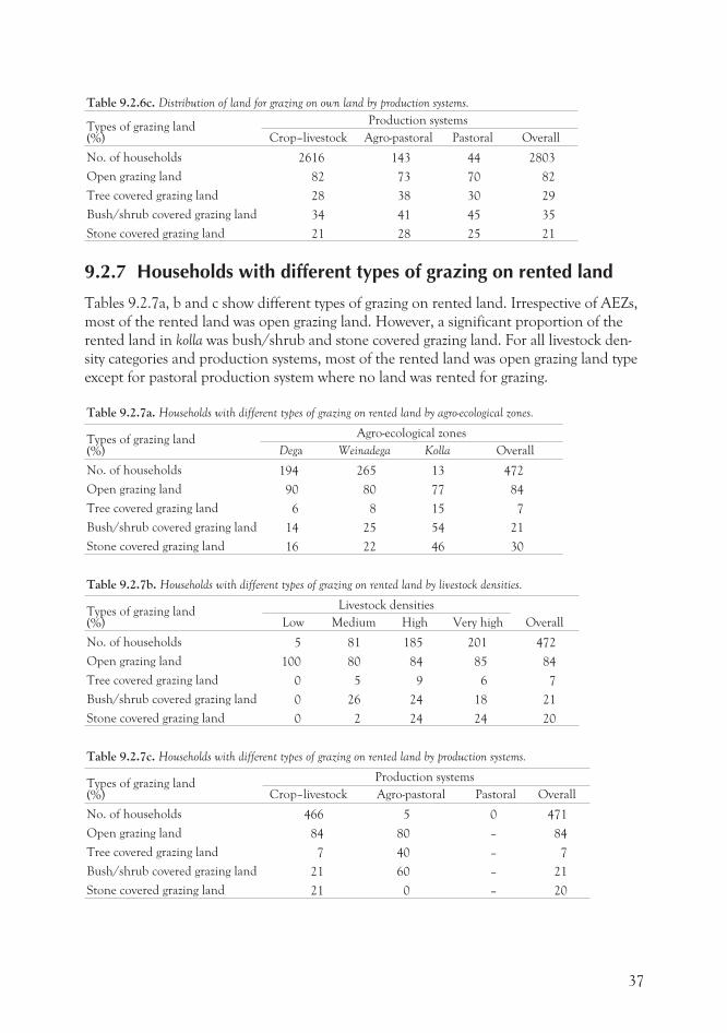
Table 9.2.6c. Distribution of land for grazing on own land by production systems.
Types of grazing land(%)
Production systems
Crop–livestock Agro-pastoral Pastoral Overall
No. of households 2616 143 44 2803
Open grazing land 82 73 70 82
Tree covered grazing land 28 38 30 29
Bush/shrub covered grazing land 34 41 45 35
Stone covered grazing land 21 28 25 21
9.2.7 Households with different types of grazing on rented land
Tables 9.2.7a, b and c show different types of grazing on rented land. Irrespective of AEZs,
most of the rented land was open grazing land. However, a significant proportion of the
rented land in kolla was bush/shrub and stone covered grazing land. For all livestock den-
sity categories and production systems, most of the rented land was open grazing land type
except for pastoral production system where no land was rented for grazing.
Table 9.2.7a. Households with different types of grazing on rented land by agro-ecological zones.
Types of grazing land(%)
Agro-ecological zones
Dega Weinadega Kolla Overall
No. of households 194 265 13 472
Open grazing land 90 80 77 84
Tree covered grazing land 6 8 15 7
Bush/shrub covered grazing land 14 25 54 21
Stone covered grazing land 16 22 46 30
Table 9.2.7b. Households with different types of grazing on rented land by livestock densities.
Types of grazing land(%)
Livestock densities
OverallLow Medium High Very high
No. of households 5 81 185 201 472
Open grazing land 100 80 84 85 84
Tree covered grazing land 0 5 9 6 7
Bush/shrub covered grazing land 0 26 24 18 21
Stone covered grazing land 0 2 24 24 20
Table 9.2.7c. Households with different types of grazing on rented land by production systems.
Types of grazing land(%)
Production systems
Crop–livestock Agro-pastoral Pastoral Overall
No. of households 466 5 0 471
Open grazing land 84 80 – 84
Tree covered grazing land 7 40 – 7
Bush/shrub covered grazing land 21 60 – 21
Stone covered grazing land 21 0 – 20
37
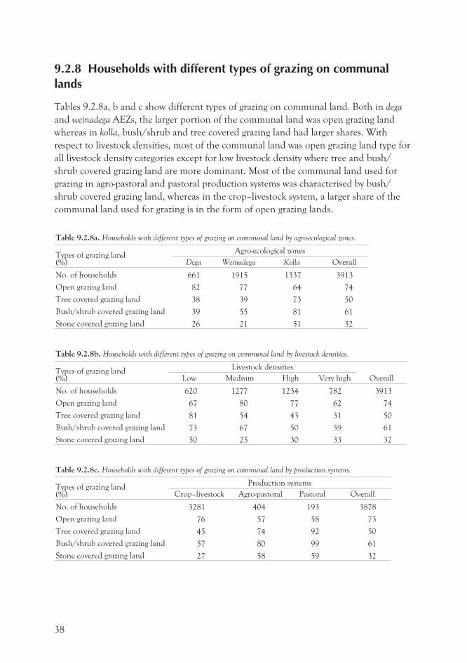
9.2.8 Households with different types of grazing on communallands
Tables 9.2.8a, b and c show different types of grazing on communal land. Both in dega
and weinadega AEZs, the larger portion of the communal land was open grazing land
whereas in kolla, bush/shrub and tree covered grazing land had larger shares. With
respect to livestock densities, most of the communal land was open grazing land type for
all livestock density categories except for low livestock density where tree and bush/
shrub covered grazing land are more dominant. Most of the communal land used for
grazing in agro-pastoral and pastoral production systems was characterised by bush/
shrub covered grazing land, whereas in the crop–livestock system, a larger share of the
communal land used for grazing is in the form of open grazing lands.
Table 9.2.8a. Households with different types of grazing on communal land by agro-ecological zones.
Types of grazing land(%)
Agro-ecological zones
Dega Weinadega Kolla Overall
No. of households 661 1915 1337 3913
Open grazing land 82 77 64 74
Tree covered grazing land 38 39 73 50
Bush/shrub covered grazing land 39 55 81 61
Stone covered grazing land 26 21 51 32
Table 9.2.8b. Households with different types of grazing on communal land by livestock densities.
Types of grazing land(%)
Livestock densities
OverallLow Medium High Very high
No. of households 620 1277 1234 782 3913
Open grazing land 67 80 77 62 74
Tree covered grazing land 81 54 43 31 50
Bush/shrub covered grazing land 73 67 50 59 61
Stone covered grazing land 50 25 30 33 32
Table 9.2.8c. Households with different types of grazing on communal land by production systems.
Types of grazing land(%)
Production systems
Crop–livestock Agro-pastoral Pastoral Overall
No. of households 3281 404 193 3878
Open grazing land 76 57 58 73
Tree covered grazing land 45 74 92 50
Bush/shrub covered grazing land 57 80 99 61
Stone covered grazing land 27 58 59 32
38
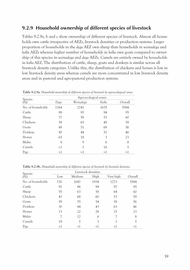
9.2.9 Household ownership of different species of livestock
Tables 9.2.9a, b and c show ownership of different species of livestock. Almost all house-
holds own cattle irrespective of AEZs, livestock densities or production systems. Larger
proportion of households in the dega AEZ own sheep than households in weinadega and
kolla AEZs whereas higher number of households in kolla own goats compared to owner-
ship of this species in weinadega and dega AEZs. Camels are entirely owned by households
in kolla AEZ. The distribution of cattle, sheep, goats and donkeys is similar across all
livestock density categories. Unlike this, the distribution of chickens and horses is low in
low livestock density areas whereas camels are more concentrated in low livestock density
areas and in pastoral and agro-pastoral production systems.
Table 9.2.9a. Household ownership of different species of livestock by agro-ecological zones.
Species(%)
Agro-ecological zones
Dega Weinadega Kolla Overall
No. of households 1164 2741 1679 5584
Cattle 98 95 94 95
Sheep 77 58 53 60
Chickens 58 65 49 59
Goats 49 51 69 56
Donkeys 45 44 51 46
Horses 65 18 3 23
Mules 9 9 6 8
Camels <1 1 16 5
Pigs <1 <1 <1 <1
Table 9.2.9b. Household ownership of different species of livestock by livestock densities.
Species(%)
Livestock densities
OverallLow Medium High Very high
No. of households 730 1647 1934 1273 5584
Cattle 92 96 94 97 95
Sheep 55 63 58 64 60
Chickens 43 68 60 53 59
Goats 59 55 54 58 56
Donkeys 30 44 43 63 46
Horses 13 22 28 25 23
Mules 7 12 6 7 8
Camels 19 5 3 1 5
Pigs <1 <1 <1 <1 <1
39
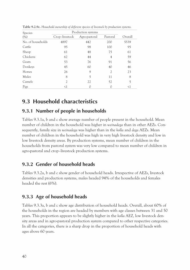
Table 9.2.9c. Household ownership of different species of livestock by production systems.
Species
(%)
Production systems
OverallCrop–livestock Agro-pastoral Pastoral
No. of households 4897 442 200 5539
Cattle 95 98 100 95
Sheep 61 48 75 61
Chickens 62 44 4 59
Goats 53 76 91 56
Donkeys 45 60 40 46
Horses 26 9 2 23
Mules 8 5 11 8
Camels 2 22 52 5
Pigs <1 0 0 <1
9.3 Household characteristics
9.3.1 Number of people in households
Tables 9.3.1a, b and c show average number of people present in the household. Mean
number of children in the household was higher in weinadega than in other AEZs. Con-
sequently, family size in weinadega was higher than in the kolla and dega AEZs. Mean
number of children in the household was high in very high livestock density and low in
low livestock density areas. By production systems, mean number of children in the
households from pastoral system was very low compared to mean number of children in
agro-pastoral and crop–livestock production systems.
9.3.2 Gender of household heads
Tables 9.3.2a, b and c show gender of household heads. Irrespective of AEZs, livestock
densities and production systems, males headed 94% of the households and females
headed the rest (6%).
9.3.3 Age of household heads
Tables 9.3.3a, b and c show age distribution of household heads. Overall, about 60% of
the households in the region are headed by members with age classes between 31 and 50
years. This proportion appears to be slightly higher in the kolla AEZ, low livestock den-
sity areas and in agro-pastoral production system compared to other respective categories.
In all the categories, there is a sharp drop in the proportion of household heads with
ages above 60 years.
40
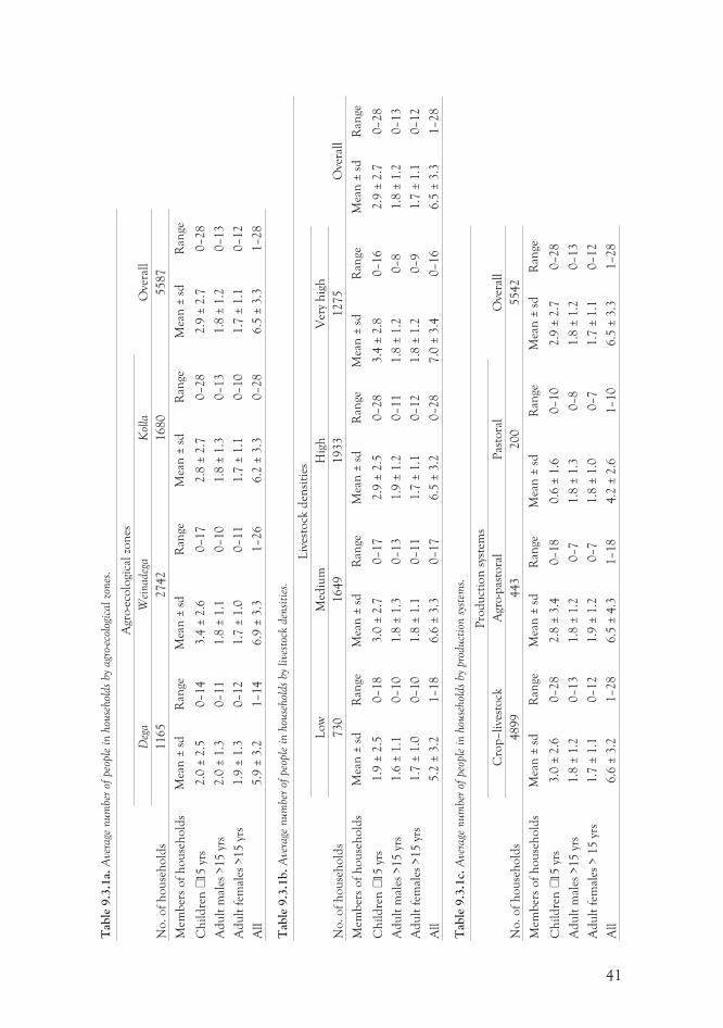
41
Tab
le9.3
.1a.
Ave
rage
num
ber
ofpe
ople
inhou
sehol
dsby
agr
o-ec
olog
icalzo
nes
.
No
.o
fh
ou
seh
old
s
Agr
o-e
colo
gica
lzo
nes
Ove
rall
Deg
aW
einadeg
aK
olla
1165
2742
1680
5587
Mem
ber
so
fh
ou
seh
old
sM
ean
±sd
Ran
geM
ean
±sd
Ran
geM
ean
±sd
Ran
geM
ean
±sd
Ran
ge
Ch
ild
ren
�15
yrs
2.0
±2.5
0–14
3.4
±2.6
0–17
2.8
±2.7
0–28
2.9
±2.7
0–28
Ad
ult
mal
es>15
yrs
2.0
±1.3
0–11
1.8
±1.1
0–10
1.8
±1.3
0–13
1.8
±1.2
0–13
Ad
ult
fem
ales
>15
yrs
1.9
±1.3
0–12
1.7
±1.0
0–11
1.7
±1.1
0–10
1.7
±1.1
0–12
All
5.9
±3.2
1–14
6.9
±3.3
1–26
6.2
±3.3
0–28
6.5
±3.3
1–28
Tab
le9.3
.1b
.A
vera
genum
ber
ofpe
ople
inhou
sehol
dsby
live
stoc
kde
nsi
ties
.
No
.o
fh
ou
seh
old
s
Liv
esto
ckd
ensi
ties
Ove
rall
Lo
wM
ediu
mH
igh
Ver
yh
igh
730
1649
1933
1275
Mem
ber
so
fh
ou
seh
old
sM
ean
±sd
Ran
geM
ean
±sd
Ran
geM
ean
±sd
Ran
geM
ean
±sd
Ran
geM
ean
±sd
Ran
ge
Ch
ild
ren
�15
yrs
1.9
±2.5
0–18
3.0
±2.7
0–17
2.9
±2.5
0–28
3.4
±2.8
0–16
2.9
±2.7
0–28
Ad
ult
mal
es>15
yrs
1.6
±1.1
0–10
1.8
±1.3
0–13
1.9
±1.2
0–11
1.8
±1.2
0–8
1.8
±1.2
0–13
Ad
ult
fem
ales
>15
yrs
1.7
±1.0
0–10
1.8
±1.1
0–11
1.7
±1.1
0–12
1.8
±1.2
0–9
1.7
±1.1
0–12
All
5.2
±3.2
1–18
6.6
±3.3
0–17
6.5
±3.2
0–28
7.0
±3.4
0–16
6.5
±3.3
1–28
Tab
le9.3
.1c.
Ave
rage
num
ber
ofpe
ople
inhou
sehol
dsby
prod
uct
ion
syst
ems.
No
.o
fh
ou
seh
old
s
Pro
du
ctio
nsy
stem
s
Ove
rall
Cro
p–li
vest
ock
Agr
o-p
asto
ral
Pas
tora
l
4899
443
200
5542
Mem
ber
so
fh
ou
seh
old
sM
ean
±sd
Ran
geM
ean
±sd
Ran
geM
ean
±sd
Ran
geM
ean
±sd
Ran
ge
Ch
ild
ren
�15
yrs
3.0
±2.6
0–28
2.8
±3.4
0–18
0.6
±1.6
0–10
2.9
±2.7
0–28
Ad
ult
mal
es>15
yrs
1.8
±1.2
0–13
1.8
±1.2
0–7
1.8
±1.3
0–8
1.8
±1.2
0–13
Ad
ult
fem
ales
>15
yrs
1.7
±1.1
0–12
1.9
±1.2
0–7
1.8
±1.0
0–7
1.7
±1.1
0–12
All
6.6
±3.2
1–28
6.5
±4.3
1–18
4.2
±2.6
1–10
6.5
±3.3
1–28
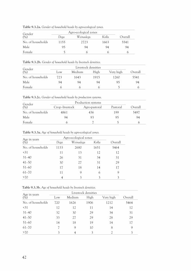
Table 9.3.2a. Gender of household heads by agro-ecological zones.
Gender(%)
Agro-ecological zones
OverallDega Weinadega Kolla
No. of households 1155 2723 1663 5541
Male 95 94 94 94
Female 5 6 6 6
Table 9.3.2b. Gender of household heads by livestock densities.
Gender(%)
Livestock densities
OverallLow Medium High Very high
No. of households 723 1643 1915 1260 5541
Male 94 94 94 95 94
Female 6 6 6 5 6
Table 9.3.2c. Gender of household heads by production systems.
Gender(%)
Production systems
OverallCrop–livestock Agro-pastoral Pastoral
No. of households 4861 436 199 5497
Male 94 93 95 94
Female 6 7 5 6
Table 9.3.3a. Age of household heads by agro-ecological zones.
Age in years(%)
Agro-ecological zones
OverallDega Weinadega Kolla
No. of households 1133 2680 1651 5464
<31 11 13 12 12
31–40 26 31 34 31
41–50 30 27 31 29
51–60 17 18 14 17
61–70 11 9 6 9
>70 4 3 3 3
Table 9.3.3b. Age of household heads by livestock densities.
Age in years(%)
Livestock densities
OverallLow Medium High Very high
No. of households 720 1626 1906 1212 5464
<31 12 12 11 14 12
31–40 32 30 29 34 31
41–50 33 27 29 28 29
51–60 14 18 19 14 17
61–70 7 9 10 8 9
>70 3 4 3 2 3
42
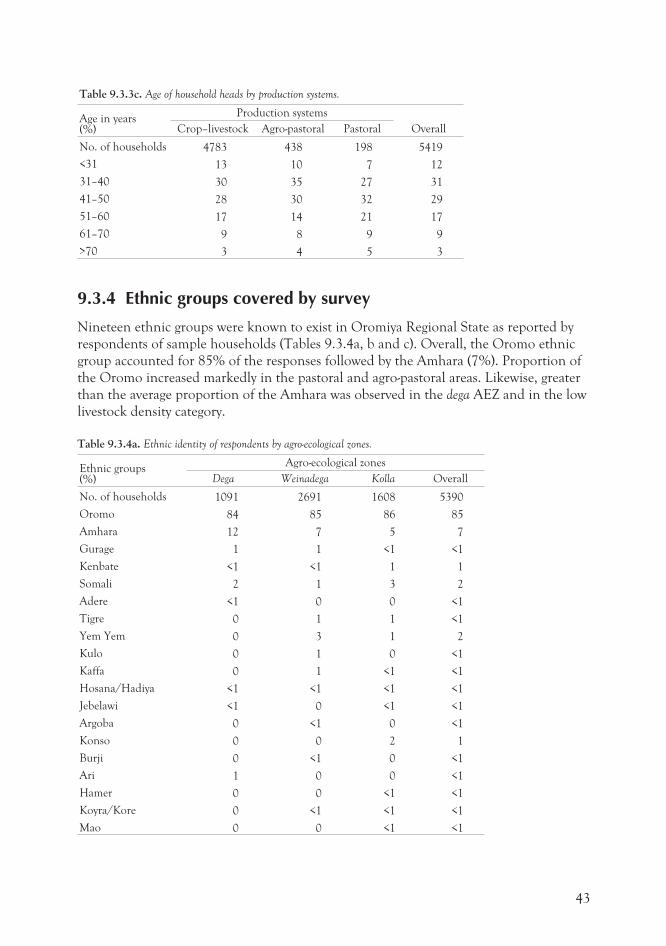
Table 9.3.3c. Age of household heads by production systems.
Age in years(%)
Production systems
OverallCrop–livestock Agro-pastoral Pastoral
No. of households 4783 438 198 5419
<31 13 10 7 12
31–40 30 35 27 31
41–50 28 30 32 29
51–60 17 14 21 17
61–70 9 8 9 9
>70 3 4 5 3
9.3.4 Ethnic groups covered by survey
Nineteen ethnic groups were known to exist in Oromiya Regional State as reported by
respondents of sample households (Tables 9.3.4a, b and c). Overall, the Oromo ethnic
group accounted for 85% of the responses followed by the Amhara (7%). Proportion of
the Oromo increased markedly in the pastoral and agro-pastoral areas. Likewise, greater
than the average proportion of the Amhara was observed in the dega AEZ and in the low
livestock density category.
Table 9.3.4a. Ethnic identity of respondents by agro-ecological zones.
Ethnic groups(%)
Agro-ecological zones
Dega Weinadega Kolla Overall
No. of households 1091 2691 1608 5390
Oromo 84 85 86 85
Amhara 12 7 5 7
Gurage 1 1 <1 <1
Kenbate <1 <1 1 1
Somali 2 1 3 2
Adere <1 0 0 <1
Tigre 0 1 1 <1
Yem Yem 0 3 1 2
Kulo 0 1 0 <1
Kaffa 0 1 <1 <1
Hosana/Hadiya <1 <1 <1 <1
Jebelawi <1 0 <1 <1
Argoba 0 <1 0 <1
Konso 0 0 2 1
Burji 0 <1 0 <1
Ari 1 0 0 <1
Hamer 0 0 <1 <1
Koyra/Kore 0 <1 <1 <1
Mao 0 0 <1 <1
43
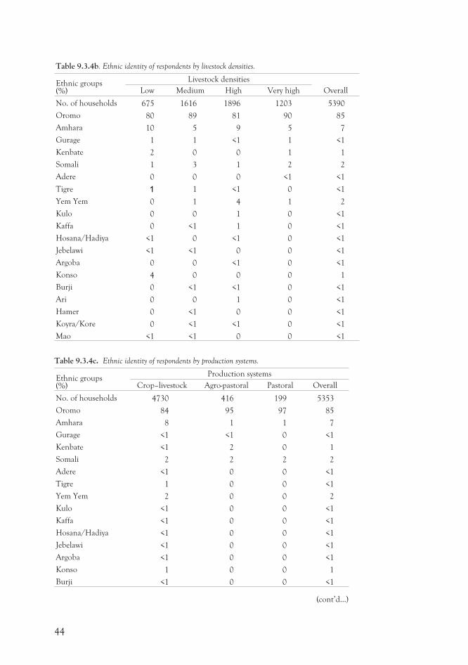
Table 9.3.4b. Ethnic identity of respondents by livestock densities.
Ethnic groups(%)
Livestock densities
OverallLow Medium High Very high
No. of households 675 1616 1896 1203 5390
Oromo 80 89 81 90 85
Amhara 10 5 9 5 7
Gurage 1 1 <1 1 <1
Kenbate 2 0 0 1 1
Somali 1 3 1 2 2
Adere 0 0 0 <1 <1
Tigre 1 1 <1 0 <1
Yem Yem 0 1 4 1 2
Kulo 0 0 1 0 <1
Kaffa 0 <1 1 0 <1
Hosana/Hadiya <1 0 <1 0 <1
Jebelawi <1 <1 0 0 <1
Argoba 0 0 <1 0 <1
Konso 4 0 0 0 1
Burji 0 <1 <1 0 <1
Ari 0 0 1 0 <1
Hamer 0 <1 0 0 <1
Koyra/Kore 0 <1 <1 0 <1
Mao <1 <1 0 0 <1
Table 9.3.4c. Ethnic identity of respondents by production systems.
Ethnic groups(%)
Production systems
Crop–livestock Agro-pastoral Pastoral Overall
No. of households 4730 416 199 5353
Oromo 84 95 97 85
Amhara 8 1 1 7
Gurage <1 <1 0 <1
Kenbate <1 2 0 1
Somali 2 2 2 2
Adere <1 0 0 <1
Tigre 1 0 0 <1
Yem Yem 2 0 0 2
Kulo <1 0 0 <1
Kaffa <1 0 0 <1
Hosana/Hadiya <1 0 0 <1
Jebelawi <1 0 0 <1
Argoba <1 0 0 <1
Konso 1 0 0 1
Burji <1 0 0 <1
44
(cont’d...)
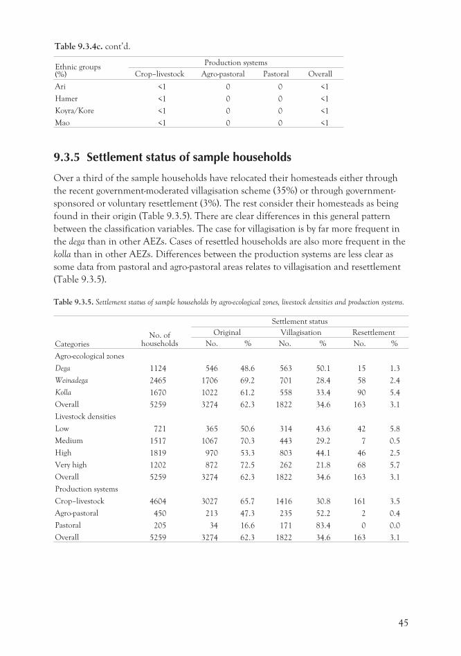
Ethnic groups(%)
Production systems
Crop–livestock Agro-pastoral Pastoral Overall
Ari <1 0 0 <1
Hamer <1 0 0 <1
Koyra/Kore <1 0 0 <1
Mao <1 0 0 <1
9.3.5 Settlement status of sample households
Over a third of the sample households have relocated their homesteads either through
the recent government-moderated villagisation scheme (35%) or through government-
sponsored or voluntary resettlement (3%). The rest consider their homesteads as being
found in their origin (Table 9.3.5). There are clear differences in this general pattern
between the classification variables. The case for villagisation is by far more frequent in
the dega than in other AEZs. Cases of resettled households are also more frequent in the
kolla than in other AEZs. Differences between the production systems are less clear as
some data from pastoral and agro-pastoral areas relates to villagisation and resettlement
(Table 9.3.5).
Table 9.3.5. Settlement status of sample households by agro-ecological zones, livestock densities and production systems.
CategoriesNo. of
households
Settlement status
Original Villagisation Resettlement
No. % No. % No. %
Agro-ecological zones
Dega 1124 546 48.6 563 50.1 15 1.3
Weinadega 2465 1706 69.2 701 28.4 58 2.4
Kolla 1670 1022 61.2 558 33.4 90 5.4
Overall 5259 3274 62.3 1822 34.6 163 3.1
Livestock densities
Low 721 365 50.6 314 43.6 42 5.8
Medium 1517 1067 70.3 443 29.2 7 0.5
High 1819 970 53.3 803 44.1 46 2.5
Very high 1202 872 72.5 262 21.8 68 5.7
Overall 5259 3274 62.3 1822 34.6 163 3.1
Production systems
Crop–livestock 4604 3027 65.7 1416 30.8 161 3.5
Agro-pastoral 450 213 47.3 235 52.2 2 0.4
Pastoral 205 34 16.6 171 83.4 0 0.0
Overall 5259 3274 62.3 1822 34.6 163 3.1
45
Table 9.3.4c. cont’d.
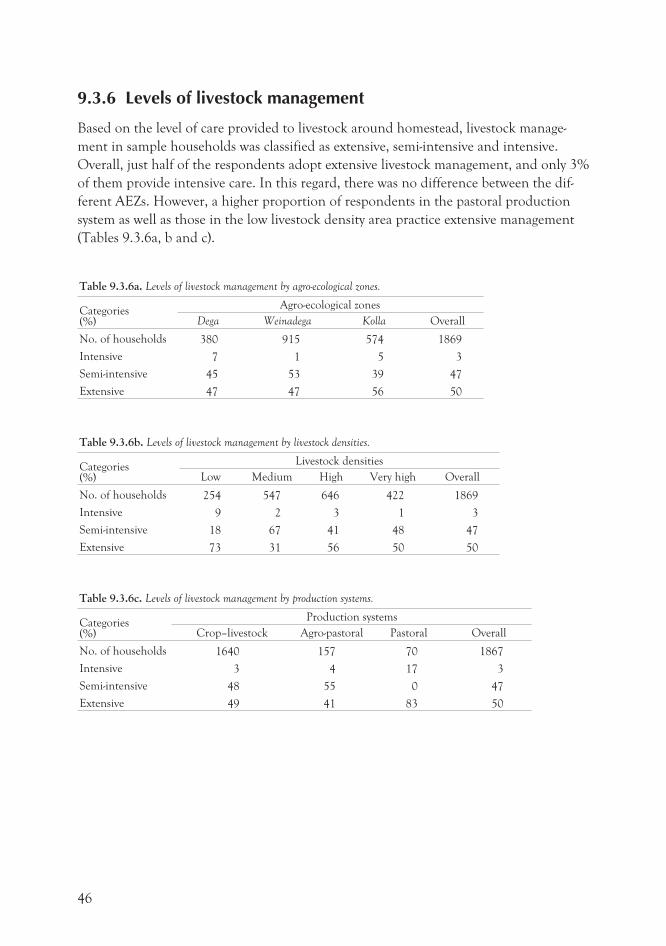
9.3.6 Levels of livestock management
Based on the level of care provided to livestock around homestead, livestock manage-
ment in sample households was classified as extensive, semi-intensive and intensive.
Overall, just half of the respondents adopt extensive livestock management, and only 3%
of them provide intensive care. In this regard, there was no difference between the dif-
ferent AEZs. However, a higher proportion of respondents in the pastoral production
system as well as those in the low livestock density area practice extensive management
(Tables 9.3.6a, b and c).
Table 9.3.6a. Levels of livestock management by agro-ecological zones.
Categories(%)
Agro-ecological zones
Dega Weinadega Kolla Overall
No. of households 380 915 574 1869
Intensive 7 1 5 3
Semi-intensive 45 53 39 47
Extensive 47 47 56 50
Table 9.3.6b. Levels of livestock management by livestock densities.
Categories(%)
Livestock densities
Low Medium High Very high Overall
No. of households 254 547 646 422 1869
Intensive 9 2 3 1 3
Semi-intensive 18 67 41 48 47
Extensive 73 31 56 50 50
Table 9.3.6c. Levels of livestock management by production systems.
Categories(%)
Production systems
Crop–livestock Agro-pastoral Pastoral Overall
No. of households 1640 157 70 1867
Intensive 3 4 17 3
Semi-intensive 48 55 0 47
Extensive 49 41 83 50
46
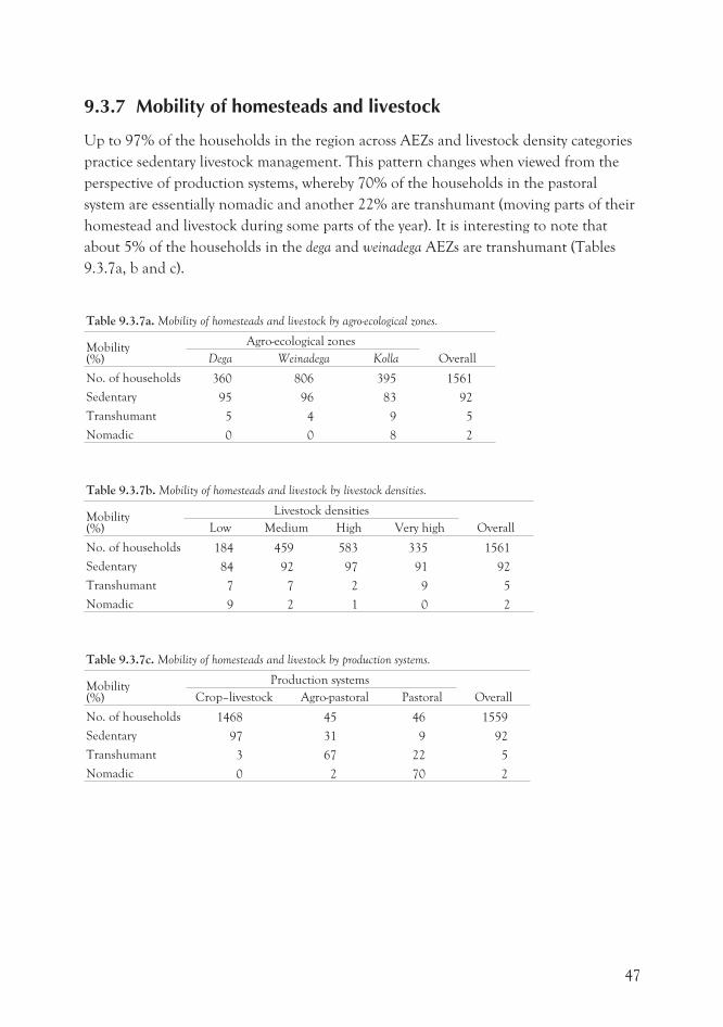
9.3.7 Mobility of homesteads and livestock
Up to 97% of the households in the region across AEZs and livestock density categories
practice sedentary livestock management. This pattern changes when viewed from the
perspective of production systems, whereby 70% of the households in the pastoral
system are essentially nomadic and another 22% are transhumant (moving parts of their
homestead and livestock during some parts of the year). It is interesting to note that
about 5% of the households in the dega and weinadega AEZs are transhumant (Tables
9.3.7a, b and c).
Table 9.3.7a. Mobility of homesteads and livestock by agro-ecological zones.
Mobility(%)
Agro-ecological zones
OverallDega Weinadega Kolla
No. of households 360 806 395 1561
Sedentary 95 96 83 92
Transhumant 5 4 9 5
Nomadic 0 0 8 2
Table 9.3.7b. Mobility of homesteads and livestock by livestock densities.
Mobility(%)
Livestock densities
OverallLow Medium High Very high
No. of households 184 459 583 335 1561
Sedentary 84 92 97 91 92
Transhumant 7 7 2 9 5
Nomadic 9 2 1 0 2
Table 9.3.7c. Mobility of homesteads and livestock by production systems.
Mobility(%)
Production systems
OverallCrop–livestock Agro-pastoral Pastoral
No. of households 1468 45 46 1559
Sedentary 97 31 9 92
Transhumant 3 67 22 5
Nomadic 0 2 70 2
47
9.4 Possibilities of using cluster analysis to characterisebreed types
This Oromiya Regional State livestock breed survey resulted in over 60 breed names of
cattle being recorded across the region (Tables 9.4a and b for cattle). It is not known
how many of these names describe distinctive breeds. Different breed names for similar
breed types may have been developed in different areas. For example, individual names
of breeds are often closely related to the clan or ethnic group to which farmers belong
or, alternatively, they may be derived from the location where the animals are raised.
Despite the variety of breed names recorded, the vast majority of cattle were reported as
belonging to the local breed (Table 9.4a). This means that it is difficult to analyse the
results to describe and compare different breed types. One possible solution is to use a
statistical method known as ‘cluster analysis’ to use the phenotypic data collected in the
survey to form different groups or clusters of animals that can then be summarised and
mapped.
Data on cattle raised in Borana Zone are used in this chapter to demonstrate this pro-
cedure. The map of Borana Zone shows the five woredas selected for the survey (Figure
9.4.1). Of these, Dire, Liben and Teltele woredas are found predominantly in kolla (low-
land), while Bore and Hagere Mariam woredas are found predominantly in dega (high-
land) agro-ecological zones with some parts of Hagere Mariam in between (weinadega).
Two-hundred and nine sets of phenotypic data were collected from households sampled
in Borana Zone. The majority of these data were collected from breeds identified by
farmers as Borana or Guji with a few Konso and Arsi breeds. From the phenotypic data
collected, 27 variables were defined for use in the cluster analysis (Table 9.4.2).
9.4.1 Methodology
The method applied starts with what is known as a Principal Component Analysis
(PCA) which calculates a few new variables (known as principal components) that are
functions of the existing 27 variables and account for most of the variation expressed by
them. Since most of the phenotypic data collected are discrete, i.e. defined according to
different categories, the method in our case incorporates what is known as a Spearman
coefficient. The PCA is followed by a method known as Agglomerative Hierarchical
Clustering (AHC) that calculates average dissimilarities between the phenotypic obser-
vations using the method of ‘Mahalanobis distance’. The ‘strong linkage’ approach is
used then to aggregate individual animal into clusters. This is done using a dendrogram
or ‘tree’ and a cut-off line can be drawn anywhere across the dendrogram to form the
required number of clusters or groups. See McGarical et al. (2000) for further details on
the methodology.
48
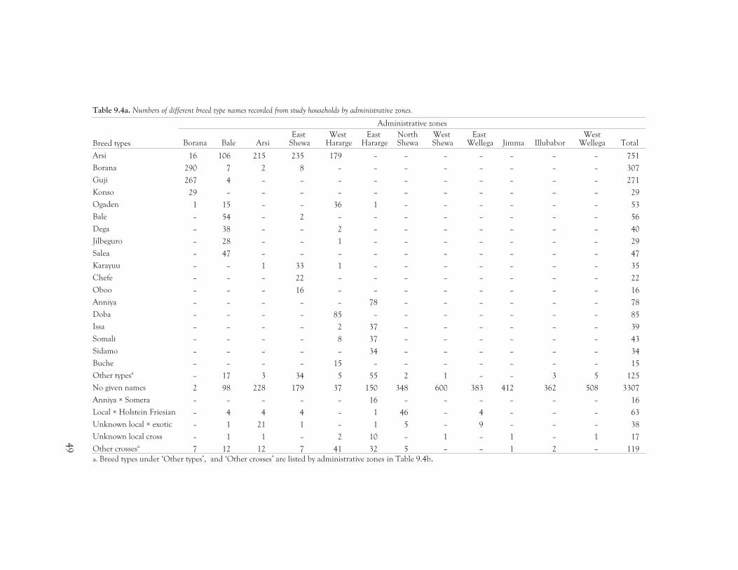
49
Table 9.4a. Numbers of different breed type names recorded from study households by administrative zones.
Breed types
Administrative zones
Borana Bale ArsiEast
ShewaWest
HarargeEast
HarargeNorthShewa
WestShewa
EastWellega Jimma Illubabor
WestWellega Total
Arsi 16 106 215 235 179 – – – – – – – 751
Borana 290 7 2 8 – – – – – – – – 307
Guji 267 4 – – – – – – – – – – 271
Konso 29 – – – – – – – – – – – 29
Ogaden 1 15 – – 36 1 – – – – – – 53
Bale – 54 – 2 – – – – – – – – 56
Dega – 38 – – 2 – – – – – – – 40
Jilbeguro – 28 – – 1 – – – – – – – 29
Salea – 47 – – – – – – – – – – 47
Karayuu – – 1 33 1 – – – – – – – 35
Chefe – – – 22 – – – – – – – – 22
Oboo – – – 16 – – – – – – – – 16
Anniya – – – – – 78 – – – – – – 78
Doba – – – – 85 – – – – – – – 85
Issa – – – – 2 37 – – – – – – 39
Somali – – – – 8 37 – – – – – – 43
Sidamo – – – – – 34 – – – – – – 34
Buche – – – – 15 – – – – – – – 15
Other typesa– 17 3 34 5 55 2 1 – – 3 5 125
No given names 2 98 228 179 37 150 348 600 383 412 362 508 3307
Anniya × Somera – – – – – 16 – – – – – – 16
Local × Holstein Friesian – 4 4 4 – 1 46 – 4 – – – 63
Unknown local × exotic – 1 21 1 – 1 5 – 9 – – – 38
Unknown local cross – 1 1 – 2 10 – 1 – 1 – 1 17
Other crossesa7 12 12 7 41 32 5 – – 1 2 – 119
a. Breed types under ‘Other types’, and ‘Other crosses’ are listed by administrative zones in Table 9.4b.
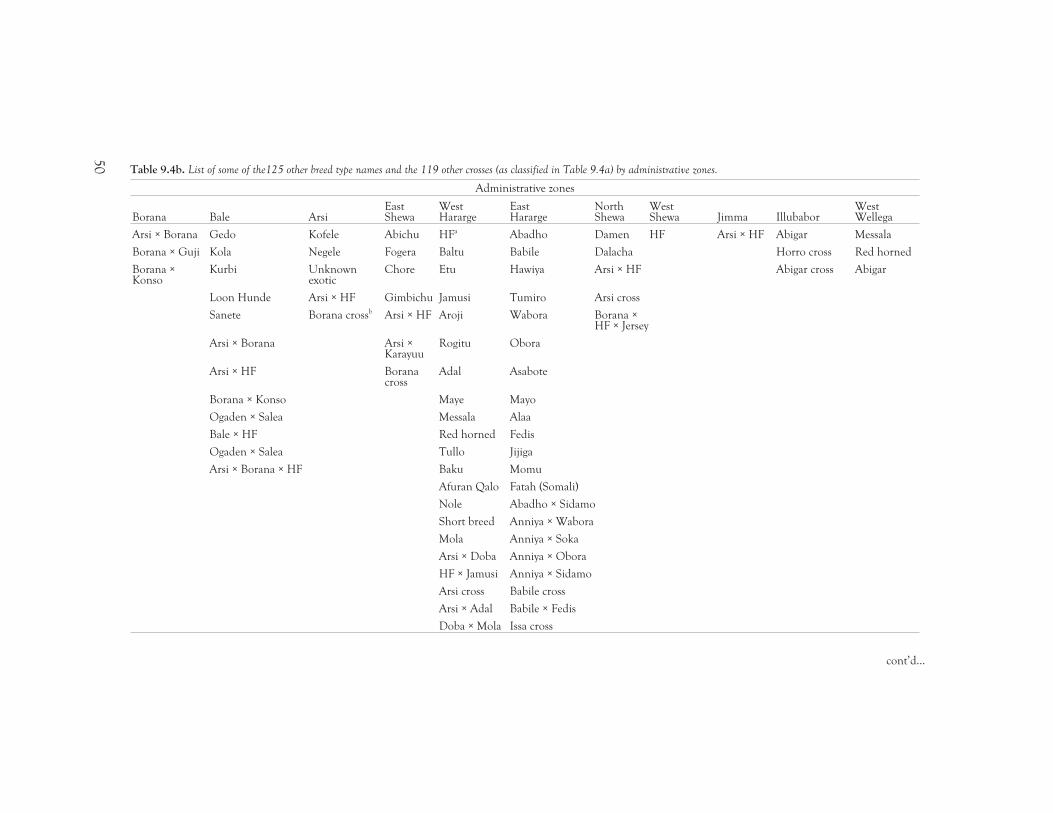
50
Table 9.4b. List of some of the125 other breed type names and the 119 other crosses (as classified in Table 9.4a) by administrative zones.
Administrative zones
Borana Bale ArsiEastShewa
WestHararge
EastHararge
NorthShewa
WestShewa Jimma Illubabor
WestWellega
Arsi × Borana Gedo Kofele Abichu HFa Abadho Damen HF Arsi × HF Abigar Messala
Borana × Guji Kola Negele Fogera Baltu Babile Dalacha Horro cross Red horned
Borana ×Konso
Kurbi Unknownexotic
Chore Etu Hawiya Arsi × HF Abigar cross Abigar
Loon Hunde Arsi × HF Gimbichu Jamusi Tumiro Arsi cross
Sanete Borana crossb Arsi × HF Aroji Wabora Borana ×HF × Jersey
Arsi × Borana Arsi ×Karayuu
Rogitu Obora
Arsi × HF Boranacross
Adal Asabote
Borana × Konso Maye Mayo
Ogaden × Salea Messala Alaa
Bale × HF Red horned Fedis
Ogaden × Salea Tullo Jijiga
Arsi × Borana × HF Baku Momu
Afuran Qalo Fatah (Somali)
Nole Abadho × Sidamo
Short breed Anniya × Wabora
Mola Anniya × Soka
Arsi × Doba Anniya × Obora
HF × Jamusi Anniya × Sidamo
Arsi cross Babile cross
Arsi × Adal Babile × Fedis
Doba × Mola Issa cross
cont’d...
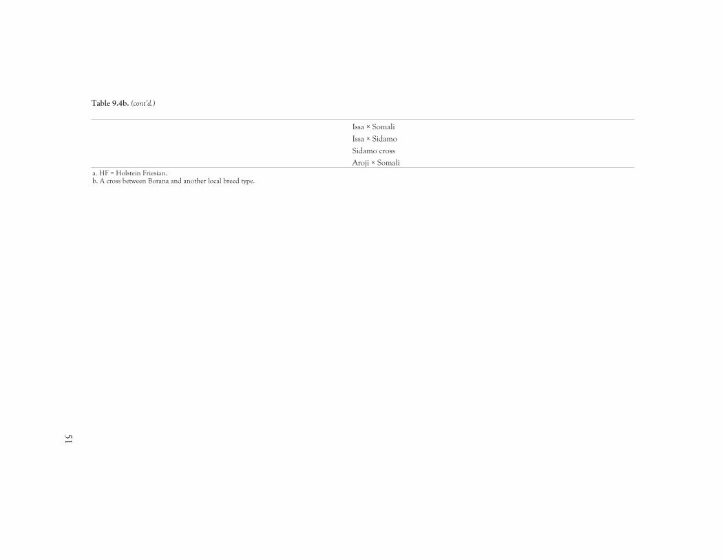
51
Issa × Somali
Issa × Sidamo
Sidamo cross
Aroji × Somali
a. HF = Holstein Friesian.b. A cross between Borana and another local breed type.
Table 9.4b. (cont’d.)
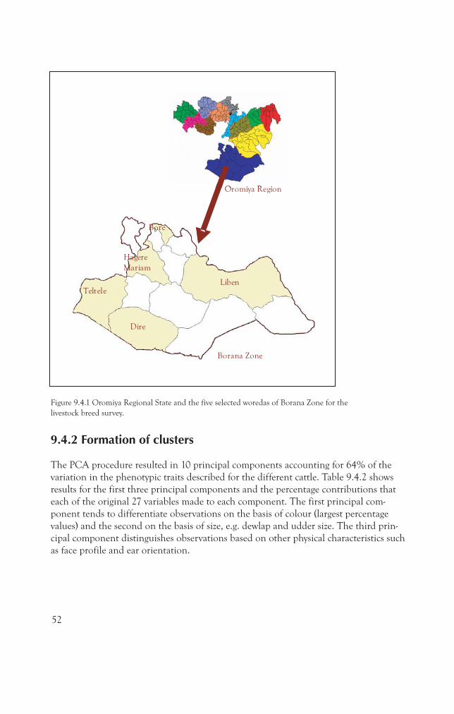
Bore
Hagere
Mariam
Liben
Dire
Teltele
Borana Zone
Oromiya Region
Bore
Hagere
Mariam
Liben
Dire
Teltele
Borana Zone
Oromiya Region
Figure 9.4.1 Oromiya Regional State and the five selected woredas of Borana Zone for the
livestock breed survey.
9.4.2 Formation of clusters
The PCA procedure resulted in 10 principal components accounting for 64% of the
variation in the phenotypic traits described for the different cattle. Table 9.4.2 shows
results for the first three principal components and the percentage contributions that
each of the original 27 variables made to each component. The first principal com-
ponent tends to differentiate observations on the basis of colour (largest percentage
values) and the second on the basis of size, e.g. dewlap and udder size. The third prin-
cipal component distinguishes observations based on other physical characteristics such
as face profile and ear orientation.
52
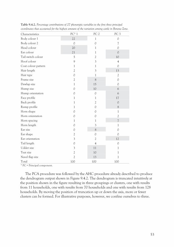
Table 9.4.2. Percentage contributions of 27 phenotypic variables to the first three principal
co-ordinates that accounted for the highest amount of the variation among cattle in Borana Zone.
Characteristics PC* 1 PC 2 PC 3
Body colour 1 22 1 0
Body colour 2 0 0 7
Head colour 20 1 0
Ear colour 21 1 0
Tail switch colour 5 2 10
Hoof colour 9 3 4
Coat colour pattern 1 1 0
Hair length 2 3 13
Hair type 0 1 2
Frame size 2 8 0
Dewlap size 1 15 0
Hump size 0 10 6
Hump orientation 0 0 6
Face profile 1 1 17
Back profile 1 2 0
Rump profile 1 0 8
Horn shape 0 0 1
Horn orientation 0 0 2
Horn spacing 1 1 7
Horn length 0 3 1
Ear size 0 8 0
Ear shape 2 0 0
Ear orientation 3 2 12
Tail length 0 4 0
Udder size 3 11 1
Teat size 2 10 1
Navel flap size 2 13 1
Total 100 100 100
* PC = Principal component.
The PCA procedure was followed by the AHC procedure already described to produce
the dendrogram output shown in Figure 9.4.2. The dendrogram is truncated intuitively at
the position shown in the figure resulting in three groupings or clusters, one with results
from 11 households, one with results from 70 households and one with results from 128
households. By moving the position of truncation up or down the axis, more or fewer
clusters can be formed. For illustrative purposes, however, we confine ourselves to three.
53
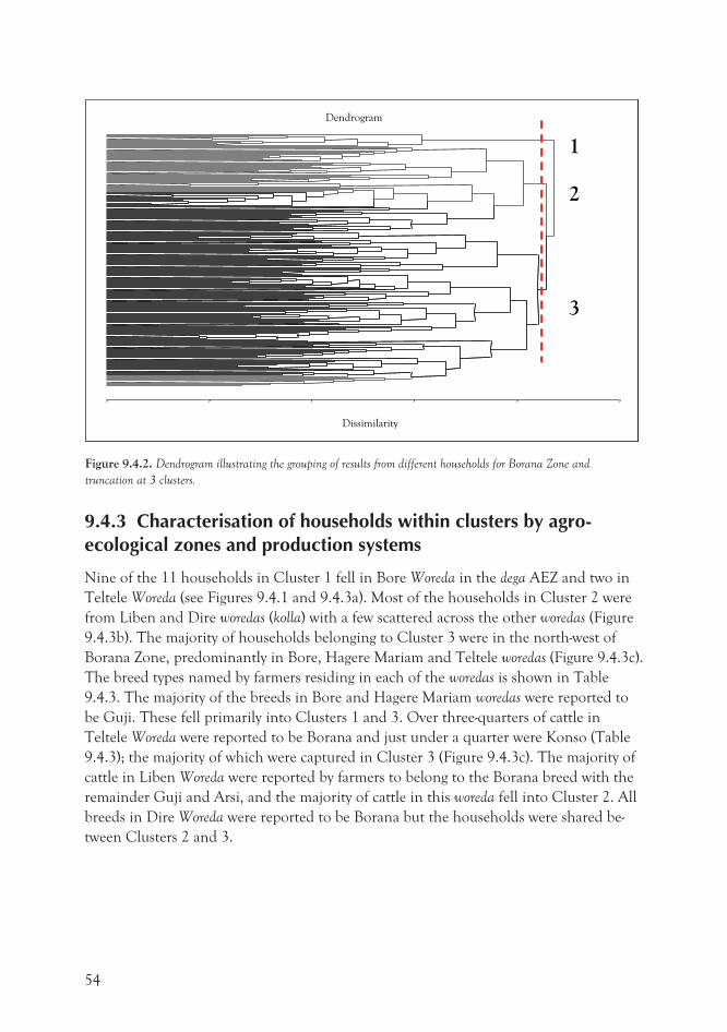
9.4.3 Characterisation of households within clusters by agro-ecological zones and production systems
Nine of the 11 households in Cluster 1 fell in Bore Woreda in the dega AEZ and two in
Teltele Woreda (see Figures 9.4.1 and 9.4.3a). Most of the households in Cluster 2 were
from Liben and Dire woredas (kolla) with a few scattered across the other woredas (Figure
9.4.3b). The majority of households belonging to Cluster 3 were in the north-west of
Borana Zone, predominantly in Bore, Hagere Mariam and Teltele woredas (Figure 9.4.3c).
The breed types named by farmers residing in each of the woredas is shown in Table
9.4.3. The majority of the breeds in Bore and Hagere Mariam woredas were reported to
be Guji. These fell primarily into Clusters 1 and 3. Over three-quarters of cattle in
Teltele Woreda were reported to be Borana and just under a quarter were Konso (Table
9.4.3); the majority of which were captured in Cluster 3 (Figure 9.4.3c). The majority of
cattle in Liben Woreda were reported by farmers to belong to the Borana breed with the
remainder Guji and Arsi, and the majority of cattle in this woreda fell into Cluster 2. All
breeds in Dire Woreda were reported to be Borana but the households were shared be-
tween Clusters 2 and 3.
54
Dissimilarity
Dendrogram
1
2
3
Dissimilarity
Dendrogram
1
2
3
Figure 9.4.2. Dendrogram illustrating the grouping of results from different households for Borana Zone and
truncation at 3 clusters.
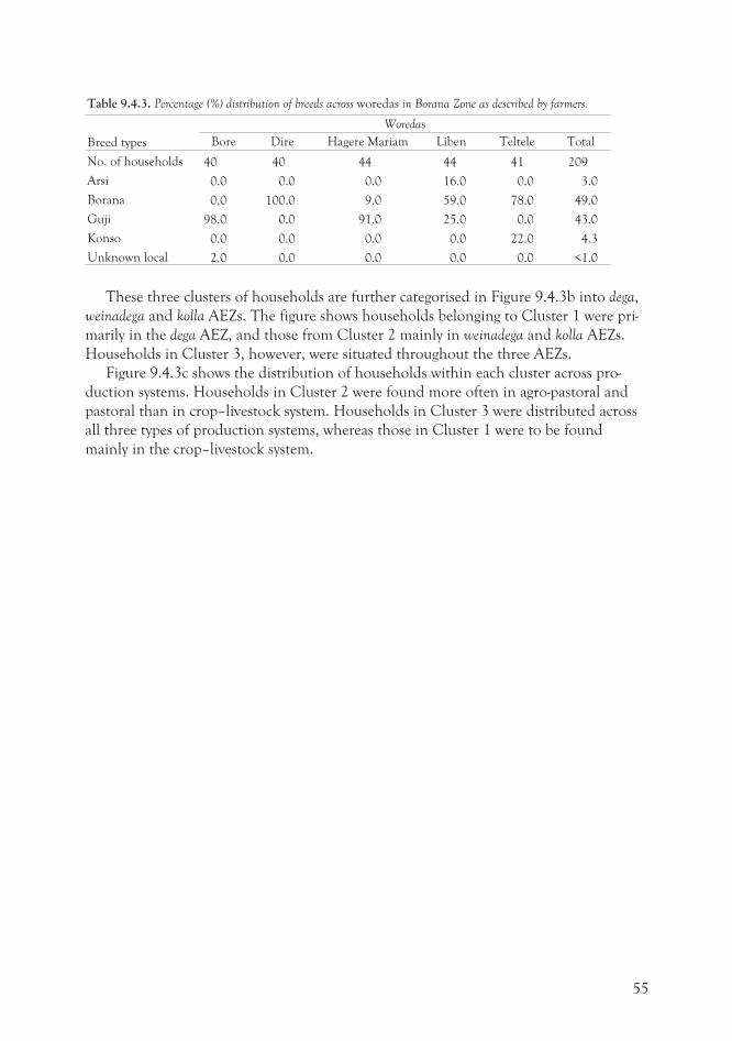
Table 9.4.3. Percentage (%) distribution of breeds across woredas in Borana Zone as described by farmers.
Breed types
Woredas
Bore Dire Hagere Mariam Liben Teltele Total
No. of households 40 40 44 44 41 209
Arsi 0.0 0.0 0.0 16.0 0.0 3.0
Borana 0.0 100.0 9.0 59.0 78.0 49.0
Guji 98.0 0.0 91.0 25.0 0.0 43.0
Konso 0.0 0.0 0.0 0.0 22.0 4.3
Unknown local 2.0 0.0 0.0 0.0 0.0 <1.0
These three clusters of households are further categorised in Figure 9.4.3b into dega,
weinadega and kolla AEZs. The figure shows households belonging to Cluster 1 were pri-
marily in the dega AEZ, and those from Cluster 2 mainly in weinadega and kolla AEZs.
Households in Cluster 3, however, were situated throughout the three AEZs.
Figure 9.4.3c shows the distribution of households within each cluster across pro-
duction systems. Households in Cluster 2 were found more often in agro-pastoral and
pastoral than in crop–livestock system. Households in Cluster 3 were distributed across
all three types of production systems, whereas those in Cluster 1 were to be found
mainly in the crop–livestock system.
55
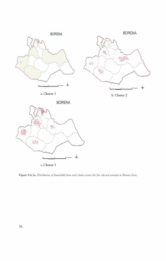
56
a. Cluster 1b. Cluster 2
c. Cluster 3
a. Cluster 1b. Cluster 2
c. Cluster 3
Figure 9.4.3a. Distribution of households from each cluster across the five selected woredas in Borana Zone.
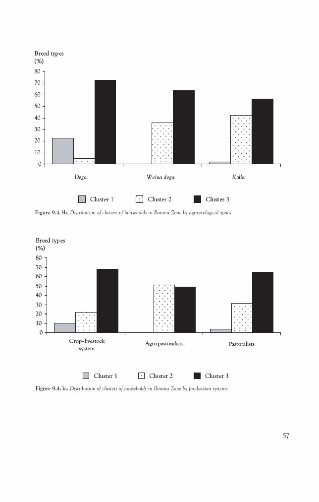
57
0
10
20
30
40
50
60
70
80
Dega Weina dega Kolla
Breed types
(%)
Cluster 1 Cluster 2 Cluster 3
0
10
20
30
40
50
60
70
80
Dega Weina dega Kolla
Breed types
(%)
Cluster 1 Cluster 2 Cluster 3
Figure 9.4.3b. Distribution of clusters of households in Borana Zone by agro-ecological zones.
0
10
20
30
40
50
60
70
80
Crop–livestock
systemAgro-pastoralists Pastoralists
Breed types
(%)
Cluster 1 Cluster 2 Cluster 3
0
10
20
30
40
50
60
70
80
Crop–livestock
systemAgro-pastoralists Pastoralists
Breed types
(%)
Cluster 1 Cluster 2 Cluster 3
Figure 9.4.3c. Distribution of clusters of households in Borana Zone by production systems.
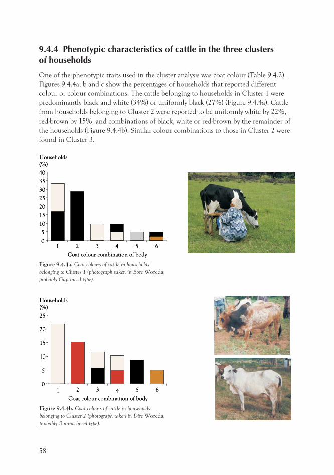
9.4.4 Phenotypic characteristics of cattle in the three clustersof households
One of the phenotypic traits used in the cluster analysis was coat colour (Table 9.4.2).
Figures 9.4.4a, b and c show the percentages of households that reported different
colour or colour combinations. The cattle belonging to households in Cluster 1 were
predominantly black and white (34%) or uniformly black (27%) (Figure 9.4.4a). Cattle
from households belonging to Cluster 2 were reported to be uniformly white by 22%,
red-brown by 15%, and combinations of black, white or red-brown by the remainder of
the households (Figure 9.4.4b). Similar colour combinations to those in Cluster 2 were
found in Cluster 3.
58
0
5
10
15
20
25
30
35
40
1 2 3 4 5 6
Households
(%)
Coat colour combination of body
0
5
10
15
20
25
30
35
40
1 2 3 4 5 6
Households
(%)
Coat colour combination of body
Figure 9.4.4a. Coat colours of cattle in households
belonging to Cluster 1 (photograph taken in Bore Woreda,
probably Guji breed type).
0
5
10
15
20
25
2 3 5 61 4
Households
(%)
Coat colour combination of body
0
5
10
15
20
25
2 3 5 61 4
Households
(%)
Coat colour combination of body
Figure 9.4.4b. Coat colours of cattle in households
belonging to Cluster 2 (photograph taken in Dire Woreda,
probably Borana breed type).
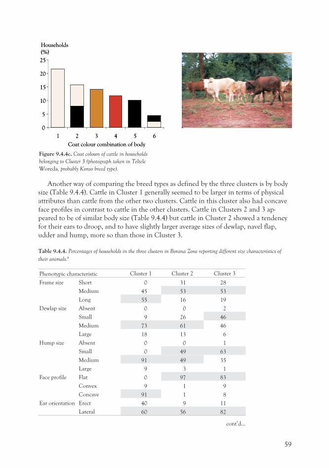
Another way of comparing the breed types as defined by the three clusters is by body
size (Table 9.4.4). Cattle in Cluster 1 generally seemed to be larger in terms of physical
attributes than cattle from the other two clusters. Cattle in this cluster also had concave
face profiles in contrast to cattle in the other clusters. Cattle in Clusters 2 and 3 ap-
peared to be of similar body size (Table 9.4.4) but cattle in Cluster 2 showed a tendency
for their ears to droop, and to have slightly larger average sizes of dewlap, navel flap,
udder and hump, more so than those in Cluster 3.
Table 9.4.4. Percentages of households in the three clusters in Borana Zone reporting different size characteristics of
their animals.a
Phenotypic characteristic Cluster 1 Cluster 2 Cluster 3
Frame size Short 0 31 28
Medium 45 53 53
Long 55 16 19
Dewlap size Absent 0 0 2
Small 9 26 46
Medium 73 61 46
Large 18 13 6
Hump size Absent 0 0 1
Small 0 49 63
Medium 91 49 35
Large 9 3 1
Face profile Flat 0 97 83
Convex 9 1 9
Concave 91 1 8
Ear orientation Erect 40 9 11
Lateral 60 56 82
59
0
10
20
25
1 2 3 4 5
5
15
6
Households
(%)
Coat colour combination of body
0
10
20
25
1 2 3 4 5
5
15
6
Households
(%)
Coat colour combination of body
Figure 9.4.4c. Coat colours of cattle in households
belonging to Cluster 3 (photograph taken in Teltele
Woreda, probably Konso breed type).
cont’d...
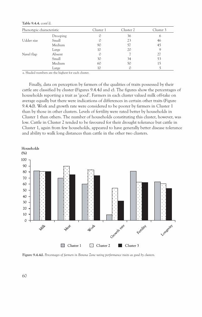
60
Figure 9.4.4d. Percentages of farmers in Borana Zone rating performance traits as good by clusters.
Milk
Mea
t
Wor
k
Gro
wth
rate
Fertili
ty
Longe
vity
0
10
20
30
40
50
60
70
80
90
100
Households
(%)
Cluster 1 Cluster 2 Cluster 3
Milk
Mea
t
Wor
k
Gro
wth
rate
Fertili
ty
Longe
vity
0
10
20
30
40
50
60
70
80
90
100
Households
(%)
Cluster 1 Cluster 2 Cluster 3
Finally, data on perception by farmers of the qualities of traits possessed by their
cattle are classified by cluster (Figures 9.4.4d and e). The figures show the percentages of
households reporting a trait as ‘good’. Farmers in each cluster valued milk off-take on
average equally but there were indications of differences in certain other traits (Figure
9.4.4d). Work and growth rate were considered to be poorer by farmers in Cluster 1
than by those in other clusters. Levels of fertility were rated better by households in
Cluster 1 than others. The number of households constituting this cluster, however, was
low. Cattle in Cluster 2 tended to be favoured for their drought tolerance but cattle in
Cluster 1, again from few households, appeared to have generally better disease tolerance
and ability to walk long distances than cattle in the other two clusters.
Drooping 0 36 6
Udder size Small 0 23 46
Medium 90 57 45
Large 10 20 9
Navel flap Absent 0 7 27
Small 30 34 53
Medium 60 50 15
Large 10 0 5
a. Shaded numbers are the highest for each cluster.
Phenotypic characteristic Cluster 1 Cluster 2 Cluster 3
Table 9.4.4. cont’d.
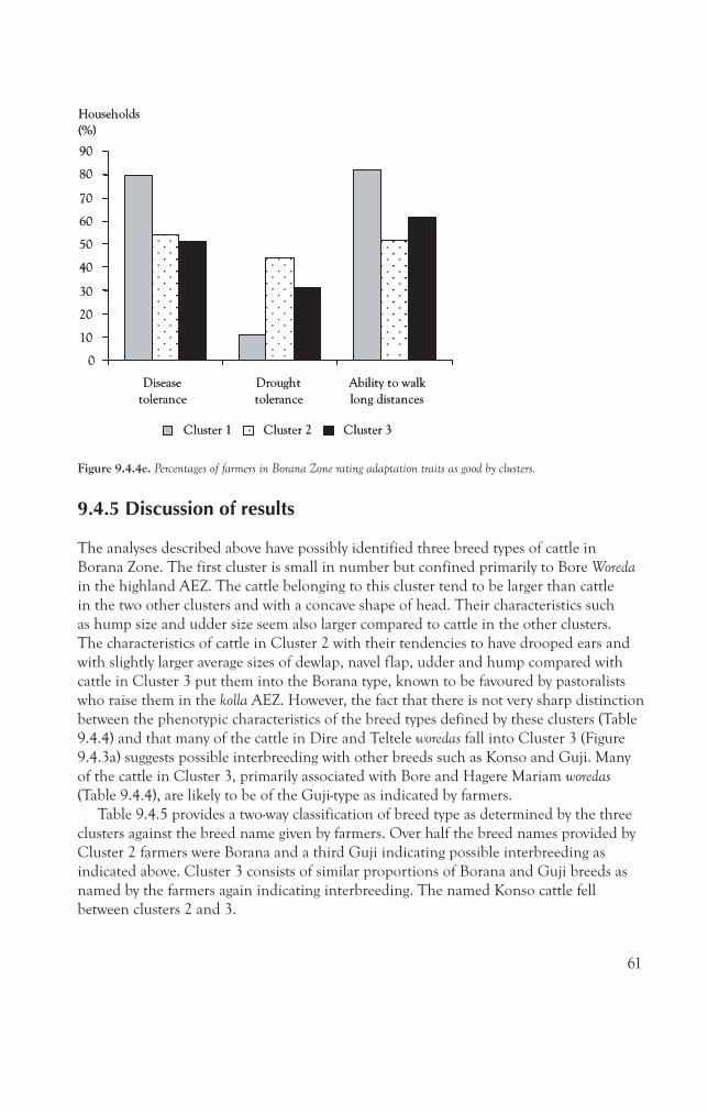
61
Figure 9.4.4e. Percentages of farmers in Borana Zone rating adaptation traits as good by clusters.
Drought
tolerance
0
10
20
30
40
50
60
70
80
90
Disease
tolerance
Ability to walk
long distances
Households
(%)
Cluster 1 Cluster 2 Cluster 3
Drought
tolerance
0
10
20
30
40
50
60
70
80
90
Disease
tolerance
Ability to walk
long distances
Households
(%)
Cluster 1 Cluster 2 Cluster 3
9.4.5 Discussion of results
The analyses described above have possibly identified three breed types of cattle in
Borana Zone. The first cluster is small in number but confined primarily to Bore Woreda
in the highland AEZ. The cattle belonging to this cluster tend to be larger than cattle
in the two other clusters and with a concave shape of head. Their characteristics such
as hump size and udder size seem also larger compared to cattle in the other clusters.
The characteristics of cattle in Cluster 2 with their tendencies to have drooped ears and
with slightly larger average sizes of dewlap, navel flap, udder and hump compared with
cattle in Cluster 3 put them into the Borana type, known to be favoured by pastoralists
who raise them in the kolla AEZ. However, the fact that there is not very sharp distinction
between the phenotypic characteristics of the breed types defined by these clusters (Table
9.4.4) and that many of the cattle in Dire and Teltele woredas fall into Cluster 3 (Figure
9.4.3a) suggests possible interbreeding with other breeds such as Konso and Guji. Many
of the cattle in Cluster 3, primarily associated with Bore and Hagere Mariam woredas
(Table 9.4.4), are likely to be of the Guji-type as indicated by farmers.
Table 9.4.5 provides a two-way classification of breed type as determined by the three
clusters against the breed name given by farmers. Over half the breed names provided by
Cluster 2 farmers were Borana and a third Guji indicating possible interbreeding as
indicated above. Cluster 3 consists of similar proportions of Borana and Guji breeds as
named by the farmers again indicating interbreeding. The named Konso cattle fell
between clusters 2 and 3.
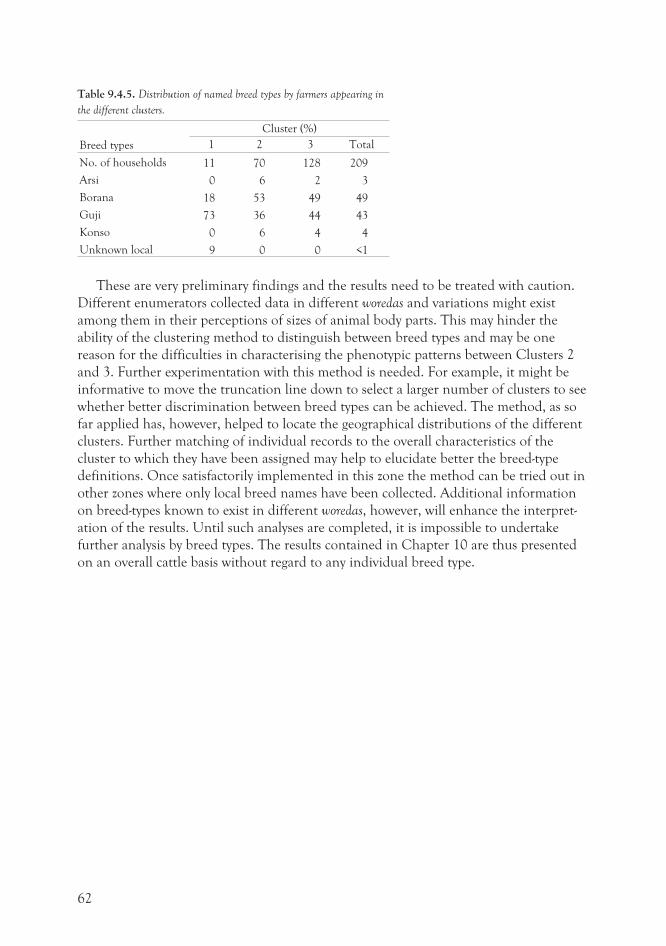
Table 9.4.5. Distribution of named breed types by farmers appearing in
the different clusters.
Breed types
Cluster (%)
1 2 3 Total
No. of households 11 70 128 209
Arsi 0 6 2 3
Borana 18 53 49 49
Guji 73 36 44 43
Konso 0 6 4 4
Unknown local 9 0 0 <1
These are very preliminary findings and the results need to be treated with caution.
Different enumerators collected data in different woredas and variations might exist
among them in their perceptions of sizes of animal body parts. This may hinder the
ability of the clustering method to distinguish between breed types and may be one
reason for the difficulties in characterising the phenotypic patterns between Clusters 2
and 3. Further experimentation with this method is needed. For example, it might be
informative to move the truncation line down to select a larger number of clusters to see
whether better discrimination between breed types can be achieved. The method, as so
far applied has, however, helped to locate the geographical distributions of the different
clusters. Further matching of individual records to the overall characteristics of the
cluster to which they have been assigned may help to elucidate better the breed-type
definitions. Once satisfactorily implemented in this zone the method can be tried out in
other zones where only local breed names have been collected. Additional information
on breed-types known to exist in different woredas, however, will enhance the interpret-
ation of the results. Until such analyses are completed, it is impossible to undertake
further analysis by breed types. The results contained in Chapter 10 are thus presented
on an overall cattle basis without regard to any individual breed type.
62
ReferencesFAO (Food and Agriculture Organization of the United Nations). 1999. The global strategy for the
management of farm animal genetic resources. Executive Brief. FAO, Rome, Italy.
McGarical K., Cushman S. and Stafford S. 2000. Multivariate statistics for wildlife and ecology
research. Springer-Verlag Inc., New York, USA. 283 pp.
Oromiya Physical Planning Department. 2000. Physical and socio-economic profiles of 180 districts of
Oromiya Region. Bureau of Planning and Economic Development, Council of the Regional
State of Oromiya, Addis Ababa, Ethiopia.
Rowlands J., Nagda S., Rege E., Mhlanga F., Dzama K., Gandiya F., Hamudikwanda H., Makuza
S., Moyo S., Matika O., Nangomasha E. and Sikosana J. 2003. The design, execution and analysis
of livestock breed surveys—A case study in Zimbabwe. A report to FAO. ILRI (International Livestock
Research Institute), Nairobi, Kenya. 211 pp.
63
10 CattleThis survey generated data on cattle from 5279 cattle-owning households across Oromiya
Regional State. These households have current holdings of over 62 thousand heads of
cattle. Only 3.5% of the households reported to have crossbred cattle in their herds, in-
dicating that almost all farmers in Oromiya Regional State maintain indigenous cattle.
As expected from extensive surveys like this, neither all households responded to all the
questions, nor all questions apply equally to all of the households. As a result, the output
tables in this chapter show different numbers of sample households. Except the tables
on herd dynamics towards the last part of this chapter, most of the tables are based on
data from 1800 households from the different categories of agro-ecological zones (AEZs),
livestock densities and production systems. Because numerous tables accommodate mul-
tiple responses to particular questions, the respective percent values may not add up to
100%.
10.1 Purposes of keeping cattleThe tables presented here show the percentages of households that reported different
purposes for which they kept cattle. As can be seen from the tables, cattle are kept for
many purposes. In any household, different species of livestock (e.g. cattle) are kept for
multiple purposes, e.g. milk and income, work and meat. Purposes for which cattle are
kept resemble more or less the breeding objectives farmers have for cattle. Data were
collected for male and female cattle separately.
10.1.1 Reasons households keep male and female cattle
Tables 10.1.1a, b and c show purposes for keeping male and female cattle by AEZs, live-
stock densities and production systems, respectively.
Irrespective of the AEZs, livestock densities and production systems, male cattle are
mainly kept for work, breeding and as a source of income, whereas female cattle are pri-
marily kept for milk and breeding. The uses of male cattle for work and breeding received
similar ratings in kola AEZ, but their use for work assumed the highest importance in the
other AEZs. The greatest differences are seen in relation to production systems (Table
10.1.1c). The need of male cattle for work was reported by only a third of pastoralists.
Instead, the keeping of males for meat ranked very high, and two-thirds of pastoralists
keep male cattle for blood. The keeping of cattle for manure is not a requirement in the
pastoral community, whereas it was considered as one purpose by 84% of crop–livestock
farmers.
64
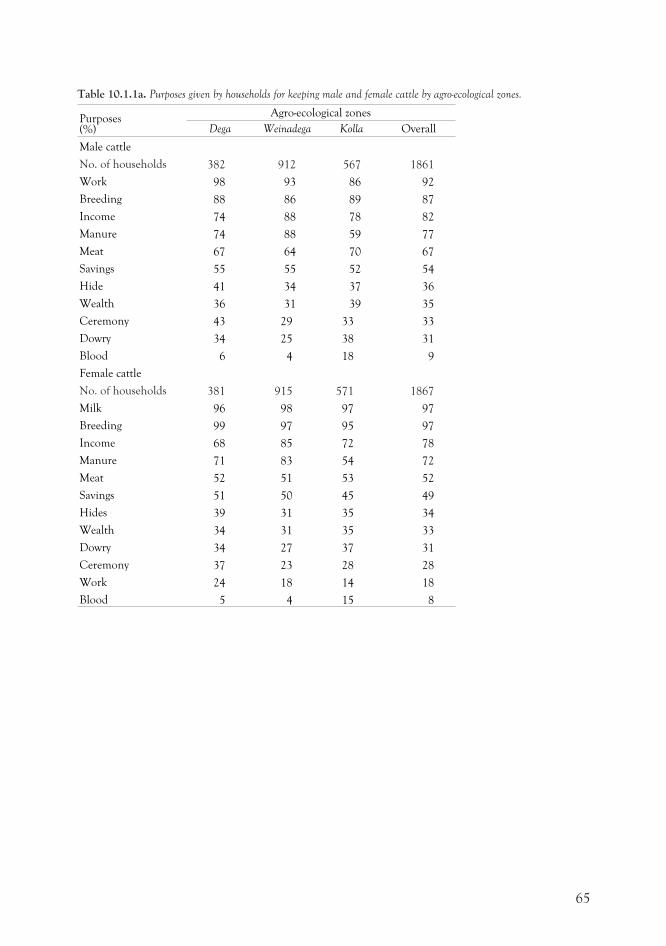
Table 10.1.1a. Purposes given by households for keeping male and female cattle by agro-ecological zones.
Purposes(%)
Agro-ecological zones
Dega Weinadega Kolla Overall
Male cattle
No. of households 382 912 567 1861
Work 98 93 86 92
Breeding 88 86 89 87
Income 74 88 78 82
Manure 74 88 59 77
Meat 67 64 70 67
Savings 55 55 52 54
Hide 41 34 37 36
Wealth 36 31 39 35
Ceremony 43 29 33 33
Dowry 34 25 38 31
Blood 6 4 18 9
Female cattle
No. of households 381 915 571 1867
Milk 96 98 97 97
Breeding 99 97 95 97
Income 68 85 72 78
Manure 71 83 54 72
Meat 52 51 53 52
Savings 51 50 45 49
Hides 39 31 35 34
Wealth 34 31 35 33
Dowry 34 27 37 31
Ceremony 37 23 28 28
Work 24 18 14 18
Blood 5 4 15 8
65
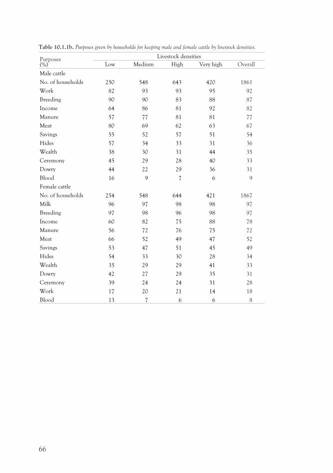
Table 10.1.1b. Purposes given by households for keeping male and female cattle by livestock densities.
Purposes(%)
Livestock densities
Low Medium High Very high Overall
Male cattle
No. of households 250 548 643 420 1861
Work 82 93 93 95 92
Breeding 90 90 83 88 87
Income 64 86 81 92 82
Manure 57 77 81 81 77
Meat 80 69 62 63 67
Savings 55 52 57 51 54
Hides 57 34 33 31 36
Wealth 38 30 31 44 35
Ceremony 45 29 28 40 33
Dowry 44 22 29 36 31
Blood 16 9 7 6 9
Female cattle
No. of households 254 548 644 421 1867
Milk 96 97 98 98 97
Breeding 97 98 96 98 97
Income 60 82 75 88 78
Manure 56 72 76 75 72
Meat 66 52 49 47 52
Savings 53 47 51 45 49
Hides 54 33 30 28 34
Wealth 35 29 29 41 33
Dowry 42 27 29 35 31
Ceremony 39 24 24 31 28
Work 17 20 21 14 18
Blood 13 7 6 6 8
66
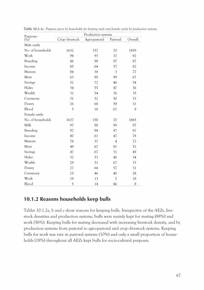
Table 10.1.1c. Purposes given by households for keeping male and female cattle by production systems.
Purposes(%)
Production systems
Crop–livestock Agro-pastoral Pastoral Overall
Male cattle
No. of households 1632 157 70 1859
Work 94 93 37 92
Breeding 86 98 97 87
Income 85 64 57 82
Manure 84 38 3 77
Meat 63 89 99 67
Savings 52 72 46 54
Hides 34 55 47 36
Wealth 31 54 76 35
Ceremony 31 52 50 33
Dowry 26 68 59 31
Blood 5 18 67 9
Female cattle
No. of households 1637 158 70 1865
Milk 97 98 99 97
Breeding 97 94 97 97
Income 80 61 47 78
Manure 78 37 4 72
Meat 49 67 81 52
Savings 47 67 31 49
Hides 32 53 40 34
Wealth 29 51 67 33
Dowry 27 64 57 31
Ceremony 25 46 40 28
Work 19 13 5 18
Blood 5 14 46 8
10.1.2 Reasons households keep bulls
Tables 10.1.2a, b and c show reasons for keeping bulls. Irrespective of the AEZs, live-
stock densities and production systems, bulls were mainly kept for mating (88%) and
work (56%). Keeping bulls for mating decreased with increasing livestock density, and by
production systems from pastoral to agro-pastoral and crop–livestock systems. Keeping
bulls for work was rare in pastoral systems (10%) and only a small proportion of house-
holds (18%) throughout all AEZs kept bulls for socio-cultural purposes.
67
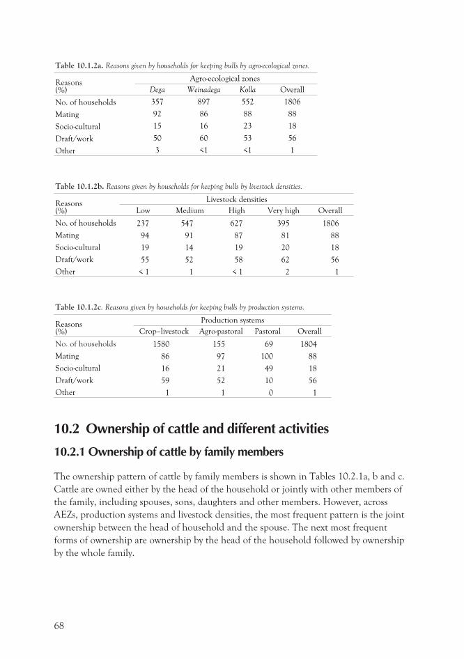
Table 10.1.2a. Reasons given by households for keeping bulls by agro-ecological zones.
Reasons(%)
Agro-ecological zones
Dega Weinadega Kolla Overall
No. of households 357 897 552 1806
Mating 92 86 88 88
Socio-cultural 15 16 23 18
Draft/work 50 60 53 56
Other 3 <1 <1 1
Table 10.1.2b. Reasons given by households for keeping bulls by livestock densities.
Reasons(%)
Livestock densities
Low Medium High Very high Overall
No. of households 237 547 627 395 1806
Mating 94 91 87 81 88
Socio-cultural 19 14 19 20 18
Draft/work 55 52 58 62 56
Other < 1 1 < 1 2 1
Table 10.1.2c. Reasons given by households for keeping bulls by production systems.
Reasons(%)
Production systems
Crop–livestock Agro-pastoral Pastoral Overall
No. of households 1580 155 69 1804
Mating 86 97 100 88
Socio-cultural 16 21 49 18
Draft/work 59 52 10 56
Other 1 1 0 1
10.2 Ownership of cattle and different activities
10.2.1 Ownership of cattle by family members
The ownership pattern of cattle by family members is shown in Tables 10.2.1a, b and c.
Cattle are owned either by the head of the household or jointly with other members of
the family, including spouses, sons, daughters and other members. However, across
AEZs, production systems and livestock densities, the most frequent pattern is the joint
ownership between the head of household and the spouse. The next most frequent
forms of ownership are ownership by the head of the household followed by ownership
by the whole family.
68
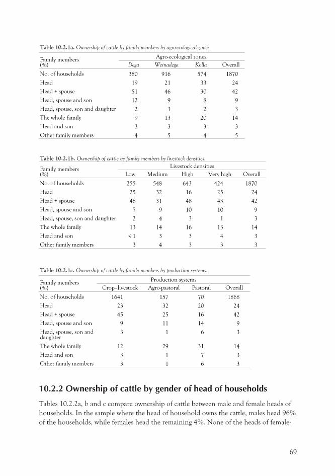
Table 10.2.1a. Ownership of cattle by family members by agro-ecological zones.
Family members(%)
Agro-ecological zones
Dega Weinadega Kolla Overall
No. of households 380 916 574 1870
Head 19 21 33 24
Head + spouse 51 46 30 42
Head, spouse and son 12 9 8 9
Head, spouse, son and daughter 2 3 2 3
The whole family 9 13 20 14
Head and son 3 3 3 3
Other family members 4 5 4 5
Table 10.2.1b. Ownership of cattle by family members by livestock densities.
Family members(%)
Livestock densities
Low Medium High Very high Overall
No. of households 255 548 643 424 1870
Head 25 32 16 25 24
Head + spouse 48 31 48 43 42
Head, spouse and son 7 9 10 10 9
Head, spouse, son and daughter 2 4 3 1 3
The whole family 13 14 16 13 14
Head and son < 1 3 3 4 3
Other family members 3 4 3 3 3
Table 10.2.1c. Ownership of cattle by family members by production systems.
Family members(%)
Production systems
Crop–livestock Agro-pastoral Pastoral Overall
No. of households 1641 157 70 1868
Head 23 32 20 24
Head + spouse 45 25 16 42
Head, spouse and son 9 11 14 9
Head, spouse, son anddaughter
3 1 6 3
The whole family 12 29 31 14
Head and son 3 1 7 3
Other family members 3 1 6 3
10.2.2 Ownership of cattle by gender of head of households
Tables 10.2.2a, b and c compare ownership of cattle between male and female heads of
households. In the sample where the head of household owns the cattle, males head 96%
of the households, while females head the remaining 4%. None of the heads of female-
69
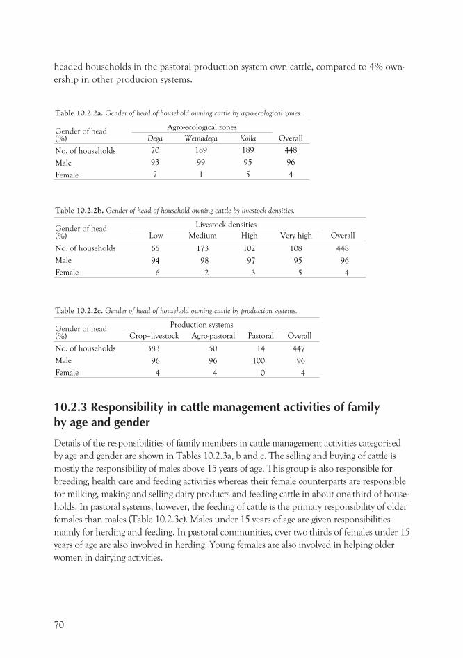
headed households in the pastoral production system own cattle, compared to 4% own-
ership in other producion systems.
Table 10.2.2a. Gender of head of household owning cattle by agro-ecological zones.
Gender of head(%)
Agro-ecological zones
Dega Weinadega Kolla Overall
No. of households 70 189 189 448
Male 93 99 95 96
Female 7 1 5 4
Table 10.2.2b. Gender of head of household owning cattle by livestock densities.
Gender of head(%)
Livestock densities
Low Medium High Very high Overall
No. of households 65 173 102 108 448
Male 94 98 97 95 96
Female 6 2 3 5 4
Table 10.2.2c. Gender of head of household owning cattle by production systems.
Gender of head(%)
Production systems
Crop–livestock Agro-pastoral Pastoral Overall
No. of households 383 50 14 447
Male 96 96 100 96
Female 4 4 0 4
10.2.3 Responsibility in cattle management activities of familyby age and gender
Details of the responsibilities of family members in cattle management activities categorised
by age and gender are shown in Tables 10.2.3a, b and c. The selling and buying of cattle is
mostly the responsibility of males above 15 years of age. This group is also responsible for
breeding, health care and feeding activities whereas their female counterparts are responsible
for milking, making and selling dairy products and feeding cattle in about one-third of house-
holds. In pastoral systems, however, the feeding of cattle is the primary responsibility of older
females than males (Table 10.2.3c). Males under 15 years of age are given responsibilities
mainly for herding and feeding. In pastoral communities, over two-thirds of females under 15
years of age are also involved in herding. Young females are also involved in helping older
women in dairying activities.
70
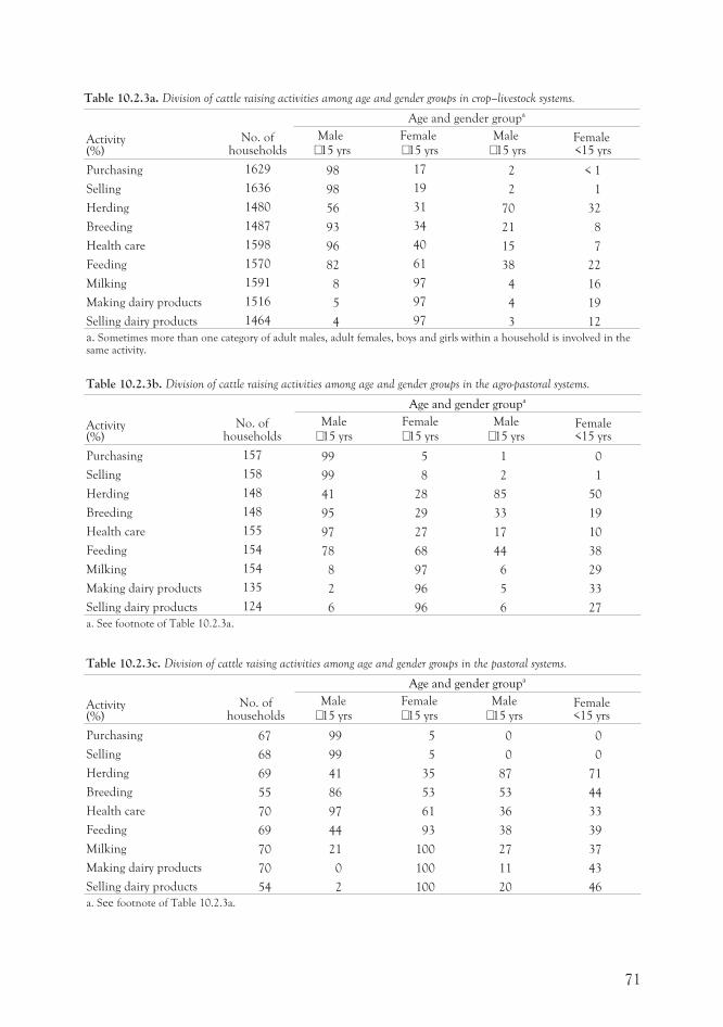
Table 10.2.3a. Division of cattle raising activities among age and gender groups in crop–livestock systems.
Activity(%)
No. ofhouseholds
Age and gender groupa
Male� 15 yrs
Female� 15 yrs
Male� 15 yrs
Female<15 yrs
Purchasing 1629 98 17 2 < 1
Selling 1636 98 19 2 1
Herding 1480 56 31 70 32
Breeding 1487 93 34 21 8
Health care 1598 96 40 15 7
Feeding 1570 82 61 38 22
Milking 1591 8 97 4 16
Making dairy products 1516 5 97 4 19
Selling dairy products 1464 4 97 3 12
a. Sometimes more than one category of adult males, adult females, boys and girls within a household is involved in thesame activity.
Table 10.2.3b. Division of cattle raising activities among age and gender groups in the agro-pastoral systems.
Activity(%)
No. ofhouseholds
Age and gender groupa
Male� 15 yrs
Female� 15 yrs
Male� 15 yrs
Female<15 yrs
Purchasing 157 99 5 1 0
Selling 158 99 8 2 1
Herding 148 41 28 85 50
Breeding 148 95 29 33 19
Health care 155 97 27 17 10
Feeding 154 78 68 44 38
Milking 154 8 97 6 29
Making dairy products 135 2 96 5 33
Selling dairy products 124 6 96 6 27
a. See footnote of Table 10.2.3a.
Table 10.2.3c. Division of cattle raising activities among age and gender groups in the pastoral systems.
Activity(%)
No. ofhouseholds
Age and gender groupa
Male� 15 yrs
Female� 15 yrs
Male� 15 yrs
Female<15 yrs
Purchasing 67 99 5 0 0
Selling 68 99 5 0 0
Herding 69 41 35 87 71
Breeding 55 86 53 53 44
Health care 70 97 61 36 33
Feeding 69 44 93 38 39
Milking 70 21 100 27 37
Making dairy products 70 0 100 11 43
Selling dairy products 54 2 100 20 46
a. See footnote of Table 10.2.3a.
71
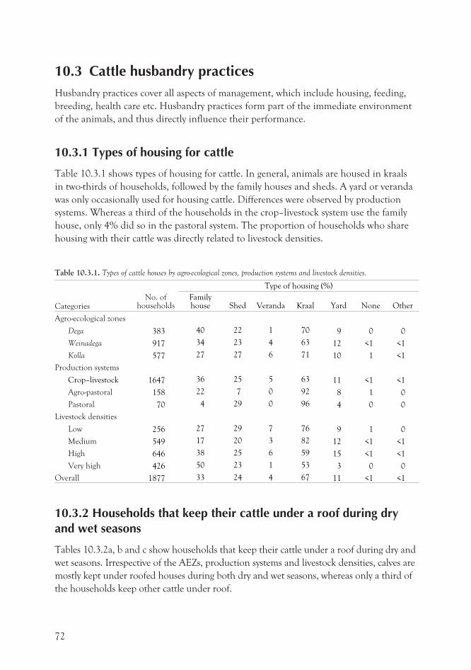
10.3 Cattle husbandry practicesHusbandry practices cover all aspects of management, which include housing, feeding,
breeding, health care etc. Husbandry practices form part of the immediate environment
of the animals, and thus directly influence their performance.
10.3.1 Types of housing for cattle
Table 10.3.1 shows types of housing for cattle. In general, animals are housed in kraals
in two-thirds of households, followed by the family houses and sheds. A yard or veranda
was only occasionally used for housing cattle. Differences were observed by production
systems. Whereas a third of the households in the crop–livestock system use the family
house, only 4% did so in the pastoral system. The proportion of households who share
housing with their cattle was directly related to livestock densities.
Table 10.3.1. Types of cattle houses by agro-ecological zones, production systems and livestock densities.
CategoriesNo. of
households
Type of housing (%)
Familyhouse Shed Veranda Kraal Yard None Other
Agro-ecological zones
Dega 383 40 22 1 70 9 0 0
Weinadega 917 34 23 4 63 12 <1 <1
Kolla 577 27 27 6 71 10 1 <1
Production systems
Crop–livestock 1647 36 25 5 63 11 <1 <1
Agro-pastoral 158 22 7 0 92 8 1 0
Pastoral 70 4 29 0 96 4 0 0
Livestock densities
Low 256 27 29 7 76 9 1 0
Medium 549 17 20 3 82 12 <1 <1
High 646 38 25 6 59 15 <1 <1
Very high 426 50 23 1 53 3 0 0
Overall 1877 33 24 4 67 11 <1 <1
10.3.2 Households that keep their cattle under a roof during dryand wet seasons
Tables 10.3.2a, b and c show households that keep their cattle under a roof during dry and
wet seasons. Irrespective of the AEZs, production systems and livestock densities, calves are
mostly kept under roofed houses during both dry and wet seasons, whereas only a third of
the households keep other cattle under roof.
72
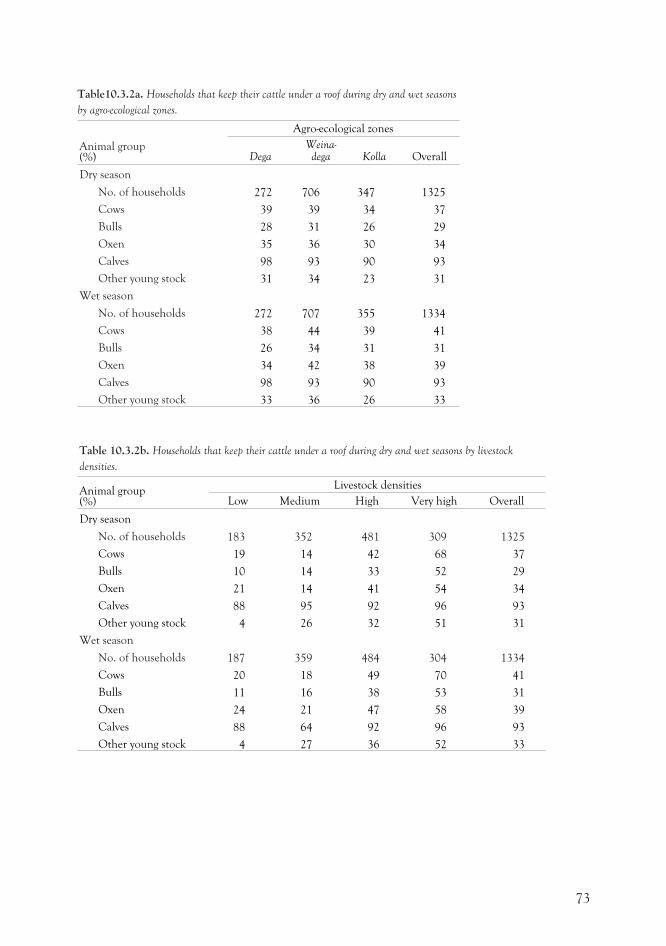
Table10.3.2a. Households that keep their cattle under a roof during dry and wet seasons
by agro-ecological zones.
Animal group(%)
Agro-ecological zones
DegaWeina-dega Kolla Overall
Dry season
No. of households 272 706 347 1325
Cows 39 39 34 37
Bulls 28 31 26 29
Oxen 35 36 30 34
Calves 98 93 90 93
Other young stock 31 34 23 31
Wet season
No. of households 272 707 355 1334
Cows 38 44 39 41
Bulls 26 34 31 31
Oxen 34 42 38 39
Calves 98 93 90 93
Other young stock 33 36 26 33
Table 10.3.2b. Households that keep their cattle under a roof during dry and wet seasons by livestock
densities.
Animal group(%)
Livestock densities
Low Medium High Very high Overall
Dry season
No. of households 183 352 481 309 1325
Cows 19 14 42 68 37
Bulls 10 14 33 52 29
Oxen 21 14 41 54 34
Calves 88 95 92 96 93
Other young stock 4 26 32 51 31
Wet season
No. of households 187 359 484 304 1334
Cows 20 18 49 70 41
Bulls 11 16 38 53 31
Oxen 24 21 47 58 39
Calves 88 64 92 96 93
Other young stock 4 27 36 52 33
73
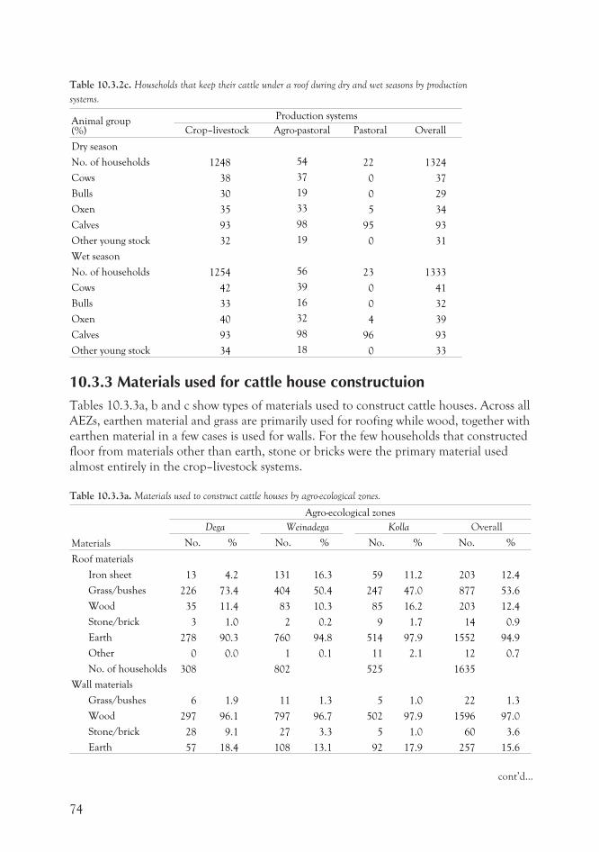
Table 10.3.2c. Households that keep their cattle under a roof during dry and wet seasons by production
systems.
Animal group(%)
Production systems
Crop–livestock Agro-pastoral Pastoral Overall
Dry season
No. of households 1248 54 22 1324
Cows 38 37 0 37
Bulls 30 19 0 29
Oxen 35 33 5 34
Calves 93 98 95 93
Other young stock 32 19 0 31
Wet season
No. of households 1254 56 23 1333
Cows 42 39 0 41
Bulls 33 16 0 32
Oxen 40 32 4 39
Calves 93 98 96 93
Other young stock 34 18 0 33
10.3.3 Materials used for cattle house constructuionTables 10.3.3a, b and c show types of materials used to construct cattle houses. Across all
AEZs, earthen material and grass are primarily used for roofing while wood, together with
earthen material in a few cases is used for walls. For the few households that constructed
floor from materials other than earth, stone or bricks were the primary material used
almost entirely in the crop–livestock systems.
Table 10.3.3a. Materials used to construct cattle houses by agro-ecological zones.
Materials
Agro-ecological zones
Dega Weinadega Kolla Overall
No. % No. % No. % No. %
Roof materials
Iron sheet 13 4.2 131 16.3 59 11.2 203 12.4
Grass/bushes 226 73.4 404 50.4 247 47.0 877 53.6
Wood 35 11.4 83 10.3 85 16.2 203 12.4
Stone/brick 3 1.0 2 0.2 9 1.7 14 0.9
Earth 278 90.3 760 94.8 514 97.9 1552 94.9
Other 0 0.0 1 0.1 11 2.1 12 0.7
No. of households 308 802 525 1635
Wall materials
Grass/bushes 6 1.9 11 1.3 5 1.0 22 1.3
Wood 297 96.1 797 96.7 502 97.9 1596 97.0
Stone/brick 28 9.1 27 3.3 5 1.0 60 3.6
Earth 57 18.4 108 13.1 92 17.9 257 15.6
74
cont’d...
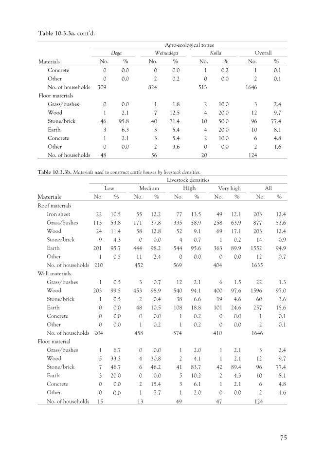
Materials
Agro-ecological zones
Dega Weinadega Kolla Overall
No. % No. % No. % No. %
Concrete 0 0.0 0 0.0 1 0.2 1 0.1
Other 0 0.0 2 0.2 0 0.0 2 0.1
No. of households 309 824 513 1646
Floor materials
Grass/bushes 0 0.0 1 1.8 2 10.0 3 2.4
Wood 1 2.1 7 12.5 4 20.0 12 9.7
Stone/brick 46 95.8 40 71.4 10 50.0 96 77.4
Earth 3 6.3 3 5.4 4 20.0 10 8.1
Concrete 1 2.1 3 5.4 2 10.0 6 4.8
Other 0 0.0 2 3.6 0 0.0 2 1.6
No. of households 48 56 20 124
Table 10.3.3b. Materials used to construct cattle houses by livestock densities.
Materials
Livestock densities
Low Medium High Very high All
No. % No. % No. % No. % No. %
Roof materials
Iron sheet 22 10.5 55 12.2 77 13.5 49 12.1 203 12.4
Grass/bushes 113 53.8 171 37.8 335 58.9 258 63.9 877 53.6
Wood 24 11.4 58 12.8 52 9.1 69 17.1 203 12.4
Stone/brick 9 4.3 0 0.0 4 0.7 1 0.2 14 0.9
Earth 201 95.7 444 98.2 544 95.6 363 89.9 1552 94.9
Other 1 0.5 11 2.4 0 0.0 0 0.0 12 0.7
No. of households 210 452 569 404 1635
Wall materials
Grass/bushes 1 0.5 3 0.7 12 2.1 6 1.5 22 1.3
Wood 203 99.5 453 98.9 540 94.1 400 97.6 1596 97.0
Stone/brick 1 0.5 2 0.4 38 6.6 19 4.6 60 3.6
Earth 0 0.0 48 10.5 108 18.8 101 24.6 257 15.6
Concrete 0 0.0 0 0.0 1 0.2 0 0.0 1 0.1
Other 0 0.0 1 0.2 1 0.2 0 0.0 2 0.1
No. of households 204 458 574 410 1646
Floor material
Grass/bushes 1 6.7 0 0.0 1 2.0 1 2.1 3 2.4
Wood 5 33.3 4 30.8 2 4.1 1 2.1 12 9.7
Stone/brick 7 46.7 6 46.2 41 83.7 42 89.4 96 77.4
Earth 3 20.0 0 0.0 5 10.2 2 4.3 10 8.1
Concrete 0 0.0 2 15.4 3 6.1 1 2.1 6 4.8
Other 0 0.0 1 7.7 1 2.0 0 0.0 2 1.6
No. of households 15 13 49 47 124
75
Table 10.3.3a. cont’d.
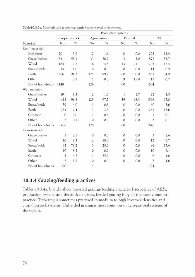
Table10.3.3c. Materials used to construct cattle houses by production systems.
Materials
Production systems
Crop–livestock Agro-pastoral Pastoral All
No. % No. % No. % No. %
Roof materials
Iron sheet 201 13.9 2 1.6 0 0.0 203 12.4
Grass/bushes 841 58.1 33 26.2 3 5.0 877 53.7
Wood 184 12.7 6 4.8 13 21.7 203 12.4
Stone/brick 14 1.0 0 0.0 0 0.0 14 0.9
Earth 1366 94.3 125 99.2 60 100.0 1551 94.9
Other 1 0.1 1 0.8 9 15.0 11 0.7
No. of households 1448 126 60 1634
Wall materials
Grass/bushes 19 1.3 2 1.6 1 1.7 22 1.3
Wood 1412 96.8 125 97.7 59 98.3 1596 97.0
Stone/brick 59 4.0 1 0.8 0 0.0 60 3.6
Earth 254 17.4 3 2.3 0 0.0 257 15.6
Concrete 0 0.0 1 0.8 0 0.0 1 0.1
Other 2 0.11 0 0.0 0 0.0 2 0.1
No. of households 1458 128 60 1646
Floor materials
Grass/bushes 3 2.5 0 0.0 0 0.0 3 2.4
Wood 10 8.3 2 50.0 0 0.0 12 9.7
Stone/brick 95 79.2 1 25.0 0 0.0 96 77.4
Earth 10 8.3 0 0.0 0 0.0 10 8.1
Concrete 5 4.2 1 25.0 0 0.0 6 4.8
Other 2 1.7 0 0.0 0 0.0 2 1.6
No. of households 120 4 124
10.3.4 Grazing/feeding practices
Tables 10.3.4a, b and c show reported grazing/feeding practices. Irrespective of AEZs,
production systems and livestock densities, herded grazing is by far the most common
practice. Tethering is sometimes practised in medium to high livestock densities and
crop–livestock systems. Unherded grazing is most common in agro-pastoral systems of
the region.
76
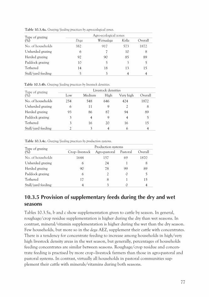
Table 10.3.4a. Grazing/feeding practices by agro-ecological zones.
Type of grazing(%)
Agro-ecological zones
Dega Weinadega Kolla Overall
No. of households 382 917 573 1872
Unherded grazing 6 7 10 8
Herded grazing 92 90 85 89
Paddock grazing 10 5 3 5
Tethered 14 18 13 15
Stall/yard feeding 5 3 4 4
Table 10.3.4b. Grazing/feeding practices by livestock densities.
Type of grazing(%)
Livestock densities
Low Medium High Very high Overall
No. of households 254 548 646 424 1872
Unherded grazing 6 11 9 2 8
Herded grazing 93 86 87 94 89
Paddock grazing 3 4 9 4 5
Tethered 3 16 20 16 15
Stall/yard feeding 2 3 4 6 4
Table 10.3.4c. Grazing/feeding practices by production systems.
Type of grazing(%)
Production systems
Crop–livestock Agro-pastoral Pastoral Overall
No. of households 1644 157 69 1870
Unherded grazing 6 24 1 8
Herded grazing 90 78 99 89
Paddock grazing 6 2 0 5
Tethered 17 8 1 15
Stall/yard feeding 4 3 0 4
10.3.5 Provision of supplementary feeds during the dry and wetseasons
Tables 10.3.5a, b and c show supplementation given to cattle by season. In general,
roughage/crop residue supplementation is higher during the dry than wet seasons. In
contrast, mineral/vitamin supplementation is higher during the wet than the dry season.
Few households, but more so in the dega AEZ, supplement their cattle with concentrates.
There is a tendency for concentrate feeding to increase among households in high/very
high livestock density areas in the wet season, but generally, percentages of households
feeding concentrates are similar between seasons. Roughage/crop residue and concen-
trate feeding is practised by more crop–livestock farmers than those in agro-pastoral and
pastoral systems. In contrast, virtually all households in pastoral communities sup-
plement their cattle with minerals/vitamins during both seasons.
77
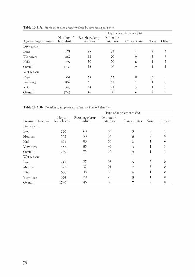
Table 10.3.5a. Provision of supplementary feeds by agro-ecological zones.
Agro-ecological zonesNumber ofhouseholds
Type of supplements (%)
Roughage/cropresidues
Minerals/vitamins Concentrates None Other
Dry season
Dega 375 75 72 14 2 2
Weinadega 867 74 70 9 1 7
Kolla 497 70 56 6 1 5
Overall 1739 73 66 9 1 5
Wet season
Dega 351 55 85 10 2 0
Weinadega 852 51 87 7 1 0
Kolla 543 34 91 3 1 0
Overall 1746 46 88 6 2 0
Table 10.3.5b. Provision of supplementary feeds by livestock densities.
Livestock densitiesNo. of
households
Type of supplements (%)
Roughage/cropresidues
Minerals/vitamins Concentrates None Other
Dry season
Low 220 68 66 5 2 7
Medium 533 58 82 6 2 8
High 604 80 65 12 1 4
Very high 382 85 46 13 1 3
Overall 1739 73 66 9 1 5
Wet season
Low 242 27 96 5 2 0
Medium 522 37 94 7 3 0
High 608 48 88 6 1 0
Very high 374 70 76 8 1 0
Overall 1746 46 88 7 2 0
78
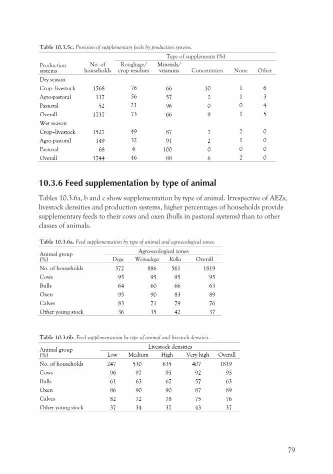
Table 10.3.5c. Provision of supplementary feeds by production systems.
Productionsystems
No. ofhouseholds
Type of supplements (%)
Roughage/crop residues
Minerals/vitamins Concentrates None Other
Dry season
Crop–livestock 1568 76 66 10 1 6
Agro-pastoral 117 56 57 2 1 3
Pastoral 52 21 96 0 0 4
Overall 1737 73 66 9 1 5
Wet season
Crop–livestock 1527 49 87 7 2 0
Agro-pastoral 149 32 91 2 1 0
Pastoral 68 6 100 0 0 0
Overall 1744 46 88 6 2 0
10.3.6 Feed supplementation by type of animal
Tables 10.3.6a, b and c show supplementation by type of animal. Irrespective of AEZs,
livestock densities and production systems, higher percentages of households provide
supplementary feeds to their cows and oxen (bulls in pastoral systems) than to other
classes of animals.
Table 10.3.6a. Feed supplementation by type of animal and agro-ecological zones.
Animal group(%)
Agro-ecological zones
Dega Weinadega Kolla Overall
No. of households 372 886 561 1819
Cows 95 95 95 95
Bulls 64 60 66 63
Oxen 95 90 83 89
Calves 83 71 79 76
Other young stock 36 35 42 37
Table 10.3.6b. Feed supplementation by type of animal and livestock densities.
Animal group(%)
Livestock densities
Low Medium High Very high Overall
No. of households 247 530 635 407 1819
Cows 96 97 95 92 95
Bulls 61 63 67 57 63
Oxen 86 90 90 87 89
Calves 82 72 78 75 76
Other young stock 37 34 37 43 37
79
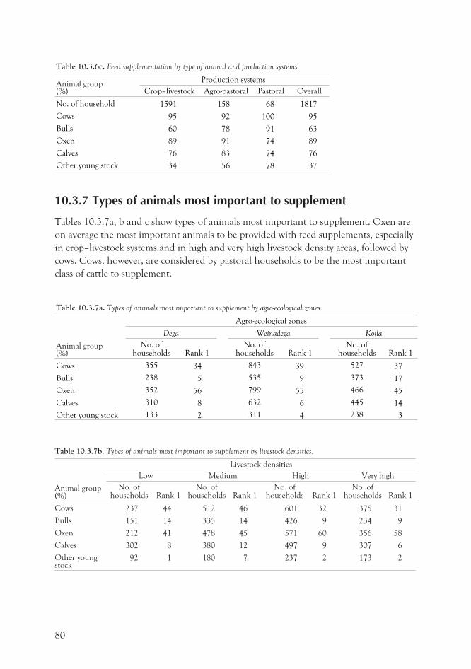
Table 10.3.6c. Feed supplementation by type of animal and production systems.
Animal group(%)
Production systems
Crop–livestock Agro-pastoral Pastoral Overall
No. of household 1591 158 68 1817
Cows 95 92 100 95
Bulls 60 78 91 63
Oxen 89 91 74 89
Calves 76 83 74 76
Other young stock 34 56 78 37
10.3.7 Types of animals most important to supplement
Tables 10.3.7a, b and c show types of animals most important to supplement. Oxen are
on average the most important animals to be provided with feed supplements, especially
in crop–livestock systems and in high and very high livestock density areas, followed by
cows. Cows, however, are considered by pastoral households to be the most important
class of cattle to supplement.
Table 10.3.7a. Types of animals most important to supplement by agro-ecological zones.
Animal group(%)
Agro-ecological zones
Dega Weinadega Kolla
No. ofhouseholds Rank 1
No. ofhouseholds Rank 1
No. ofhouseholds Rank 1
Cows 355 34 843 39 527 37
Bulls 238 5 535 9 373 17
Oxen 352 56 799 55 466 45
Calves 310 8 632 6 445 14
Other young stock 133 2 311 4 238 3
Table 10.3.7b. Types of animals most important to supplement by livestock densities.
Animal group(%)
Livestock densities
Low Medium High Very high
No. ofhouseholds Rank 1
No. ofhouseholds Rank 1
No. ofhouseholds Rank 1
No. ofhouseholds Rank 1
Cows 237 44 512 46 601 32 375 31
Bulls 151 14 335 14 426 9 234 9
Oxen 212 41 478 45 571 60 356 58
Calves 302 8 380 12 497 9 307 6
Other youngstock
92 1 180 7 237 2 173 2
80
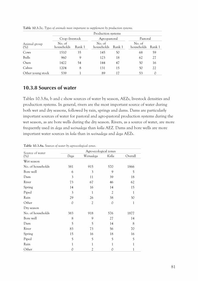
Table 10.3.7c. Types of animals most important to supplement by production systems.
Animal group(%)
Production systems
Crop–livestock Agro-pastoral Pastoral
No. ofhouseholds Rank 1
No. ofhouseholds Rank 1
No. ofhouseholds Rank 1
Cows 1510 35 145 50 68 59
Bulls 960 9 123 18 62 27
Oxen 1422 54 144 47 50 16
Calves 1204 8 131 15 50 22
Other young stock 539 1 89 17 53 0
10.3.8 Sources of water
Tables 10.3.8a, b and c show sources of water by season, AEZs, livestock densities and
production systems. In general, rivers are the most important source of water during
both wet and dry seasons, followed by rain, springs and dams. Dams are particularly
important sources of water for pastoral and agro-pastoral production systems during the
wet season, as are bore wells during the dry season. Rivers, as a source of water, are more
frequently used in dega and weinadega than kolla AEZ. Dams and bore wells are more
important water sources in kola than in weinadega and dega AEZs.
Table 10.3.8a. Sources of water by agro-ecological zones.
Source of water(%)
Agro-ecological zones
Dega Weinadega Kolla Overall
Wet season
No. of households 381 915 570 1866
Bore well 6 3 9 5
Dam 3 11 39 18
River 73 67 46 62
Spring 14 16 14 15
Piped 3 1 2 1
Rain 29 26 38 30
Other 0 2 0 1
Dry season
No. of households 383 918 576 1877
Bore well 8 9 27 14
Dam 5 5 14 8
River 83 73 56 70
Spring 15 16 18 16
Piped 5 5 5 5
Rain 1 1 1 1
Other 0 2 0 1
81
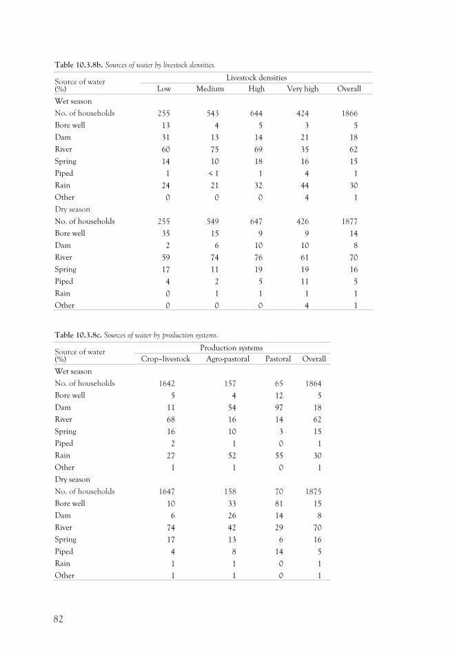
Table 10.3.8b. Sources of water by livestock densities.
Source of water(%)
Livestock densities
Low Medium High Very high Overall
Wet season
No. of households 255 543 644 424 1866
Bore well 13 4 5 3 5
Dam 31 13 14 21 18
River 60 75 69 35 62
Spring 14 10 18 16 15
Piped 1 < 1 1 4 1
Rain 24 21 32 44 30
Other 0 0 0 4 1
Dry season
No. of households 255 549 647 426 1877
Bore well 35 15 9 9 14
Dam 2 6 10 10 8
River 59 74 76 61 70
Spring 17 11 19 19 16
Piped 4 2 5 11 5
Rain 0 1 1 1 1
Other 0 0 0 4 1
Table 10.3.8c. Sources of water by production systems.
Source of water(%)
Production systems
Crop–livestock Agro-pastoral Pastoral Overall
Wet season
No. of households 1642 157 65 1864
Bore well 5 4 12 5
Dam 11 54 97 18
River 68 16 14 62
Spring 16 10 3 15
Piped 2 1 0 1
Rain 27 52 55 30
Other 1 1 0 1
Dry season
No. of households 1647 158 70 1875
Bore well 10 33 81 15
Dam 6 26 14 8
River 74 42 29 70
Spring 17 13 6 16
Piped 4 8 14 5
Rain 1 1 0 1
Other 1 1 0 1
82
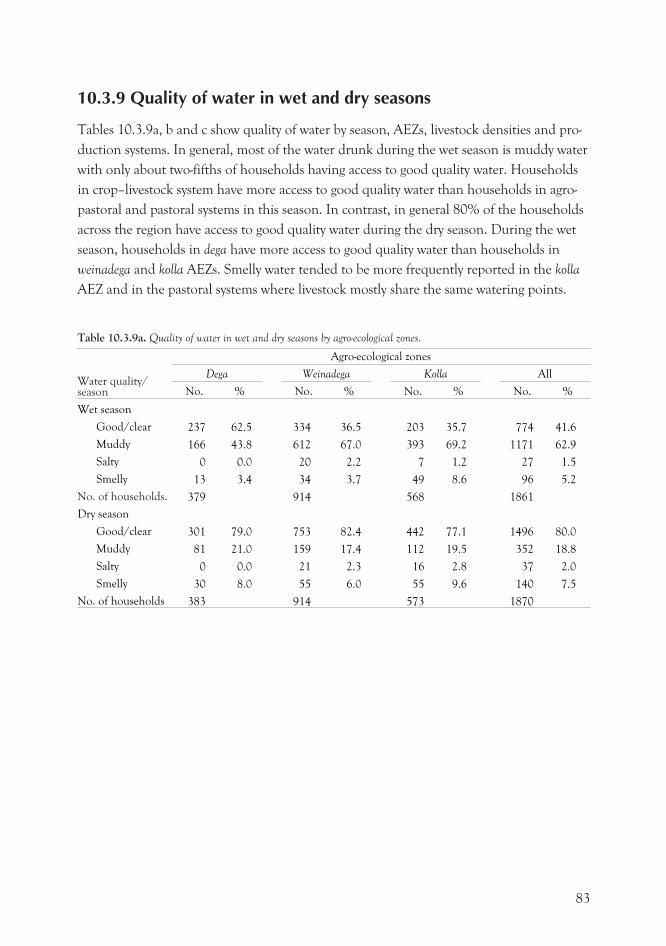
10.3.9 Quality of water in wet and dry seasons
Tables 10.3.9a, b and c show quality of water by season, AEZs, livestock densities and pro-
duction systems. In general, most of the water drunk during the wet season is muddy water
with only about two-fifths of households having access to good quality water. Households
in crop–livestock system have more access to good quality water than households in agro-
pastoral and pastoral systems in this season. In contrast, in general 80% of the households
across the region have access to good quality water during the dry season. During the wet
season, households in dega have more access to good quality water than households in
weinadega and kolla AEZs. Smelly water tended to be more frequently reported in the kolla
AEZ and in the pastoral systems where livestock mostly share the same watering points.
Table 10.3.9a. Quality of water in wet and dry seasons by agro-ecological zones.
Water quality/season
Agro-ecological zones
Dega Weinadega Kolla All
No. % No. % No. % No. %
Wet season
Good/clear 237 62.5 334 36.5 203 35.7 774 41.6
Muddy 166 43.8 612 67.0 393 69.2 1171 62.9
Salty 0 0.0 20 2.2 7 1.2 27 1.5
Smelly 13 3.4 34 3.7 49 8.6 96 5.2
No. of households. 379 914 568 1861
Dry season
Good/clear 301 79.0 753 82.4 442 77.1 1496 80.0
Muddy 81 21.0 159 17.4 112 19.5 352 18.8
Salty 0 0.0 21 2.3 16 2.8 37 2.0
Smelly 30 8.0 55 6.0 55 9.6 140 7.5
No. of households 383 914 573 1870
83
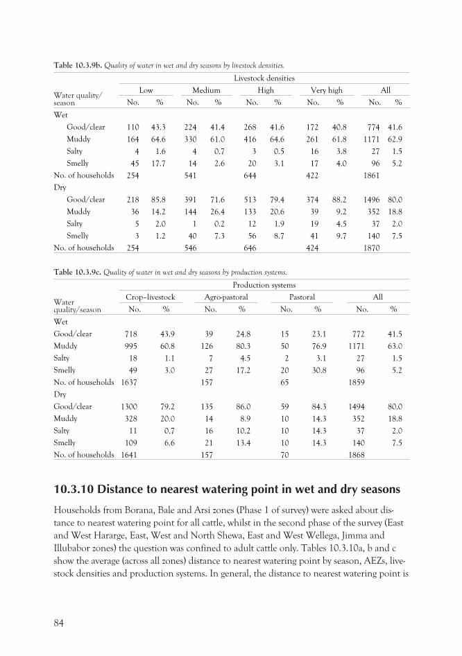
Table 10.3.9b. Quality of water in wet and dry seasons by livestock densities.
Water quality/season
Livestock densities
Low Medium High Very high All
No. % No. % No. % No. % No. %
Wet
Good/clear 110 43.3 224 41.4 268 41.6 172 40.8 774 41.6
Muddy 164 64.6 330 61.0 416 64.6 261 61.8 1171 62.9
Salty 4 1.6 4 0.7 3 0.5 16 3.8 27 1.5
Smelly 45 17.7 14 2.6 20 3.1 17 4.0 96 5.2
No. of households 254 541 644 422 1861
Dry
Good/clear 218 85.8 391 71.6 513 79.4 374 88.2 1496 80.0
Muddy 36 14.2 144 26.4 133 20.6 39 9.2 352 18.8
Salty 5 2.0 1 0.2 12 1.9 19 4.5 37 2.0
Smelly 3 1.2 40 7.3 56 8.7 41 9.7 140 7.5
No. of households 254 546 646 424 1870
Table 10.3.9c. Quality of water in wet and dry seasons by production systems.
Waterquality/season
Production systems
Crop–livestock Agro-pastoral Pastoral All
No. % No. % No. % No. %
Wet
Good/clear 718 43.9 39 24.8 15 23.1 772 41.5
Muddy 995 60.8 126 80.3 50 76.9 1171 63.0
Salty 18 1.1 7 4.5 2 3.1 27 1.5
Smelly 49 3.0 27 17.2 20 30.8 96 5.2
No. of households 1637 157 65 1859
Dry
Good/clear 1300 79.2 135 86.0 59 84.3 1494 80.0
Muddy 328 20.0 14 8.9 10 14.3 352 18.8
Salty 11 0.7 16 10.2 10 14.3 37 2.0
Smelly 109 6.6 21 13.4 10 14.3 140 7.5
No. of households 1641 157 70 1868
10.3.10 Distance to nearest watering point in wet and dry seasons
Households from Borana, Bale and Arsi zones (Phase 1 of survey) were asked about dis-
tance to nearest watering point for all cattle, whilst in the second phase of the survey (East
and West Hararge, East, West and North Shewa, East and West Wellega, Jimma and
Illubabor zones) the question was confined to adult cattle only. Tables 10.3.10a, b and c
show the average (across all zones) distance to nearest watering point by season, AEZs, live-
stock densities and production systems. In general, the distance to nearest watering point is
84
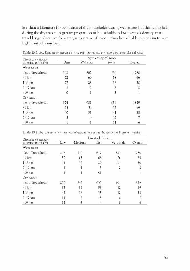
less than a kilometre for two-thirds of the households during wet season but this fell to half
during the dry season. A greater proportion of households in low livestock density areas
travel longer distances for water, irrespective of season, than households in medium to very
high livestock densities.
Table 10.3.10a. Distance to nearest watering point in wet and dry seasons by agro-ecological zones.
Distance to nearestwatering point (%)
Agro-ecological zones
Dega Weinadega Kolla Overall
Wet season
No. of households 362 882 536 1780
<1 km 72 69 58 66
1–5 km 27 28 36 30
6–10 km 2 2 3 2
>10 km 0 1 3 1
Dry season
No. of households 374 901 554 1829
<1 km 55 56 33 49
1–5 km 40 35 41 38
6–10 km 5 4 15 7
>10 km <1 5 11 6
Table 10.3.10b. Distance to nearest watering point in wet and dry seasons by livestock densities.
Distance to nearestwatering point (%)
Livestock densities
Low Medium High Very high Overall
Wet season
No. of households 246 530 617 387 1780
<1 km 50 65 68 76 66
1–5 km 41 32 29 21 30
6–10 km 4 1 3 2 2
>10 km 4 1 <1 1 1
Dry season
No. of households 250 543 635 401 1829
<1 km 35 56 53 42 49
1–5 km 42 36 35 42 38
6–10 km 11 5 8 8 7
>10 km 12 3 4 8 6
85
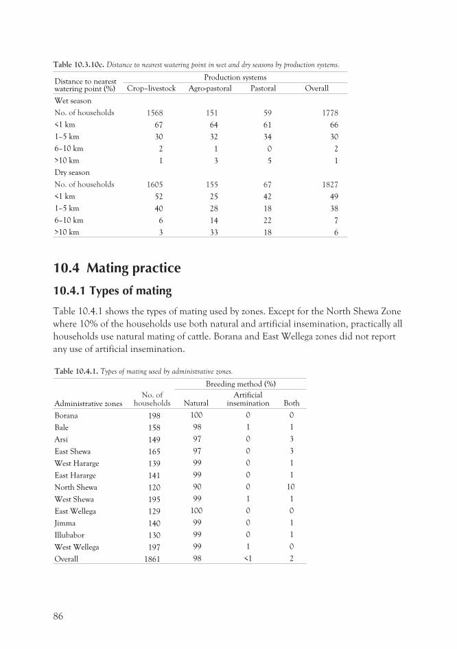
Table 10.3.10c. Distance to nearest watering point in wet and dry seasons by production systems.
Distance to nearestwatering point (%)
Production systems
Crop–livestock Agro-pastoral Pastoral Overall
Wet season
No. of households 1568 151 59 1778
<1 km 67 64 61 66
1–5 km 30 32 34 30
6–10 km 2 1 0 2
>10 km 1 3 5 1
Dry season
No. of households 1605 155 67 1827
<1 km 52 25 42 49
1–5 km 40 28 18 38
6–10 km 6 14 22 7
>10 km 3 33 18 6
10.4 Mating practice
10.4.1 Types of mating
Table 10.4.1 shows the types of mating used by zones. Except for the North Shewa Zone
where 10% of the households use both natural and artificial insemination, practically all
households use natural mating of cattle. Borana and East Wellega zones did not report
any use of artificial insemination.
Table 10.4.1. Types of mating used by administrative zones.
Administrative zonesNo. of
households
Breeding method (%)
NaturalArtificial
insemination Both
Borana 198 100 0 0
Bale 158 98 1 1
Arsi 149 97 0 3
East Shewa 165 97 0 3
West Hararge 139 99 0 1
East Hararge 141 99 0 1
North Shewa 120 90 0 10
West Shewa 195 99 1 1
East Wellega 129 100 0 0
Jimma 140 99 0 1
Illubabor 130 99 0 1
West Wellega 197 99 1 0
Overall 1861 98 <1 2
86
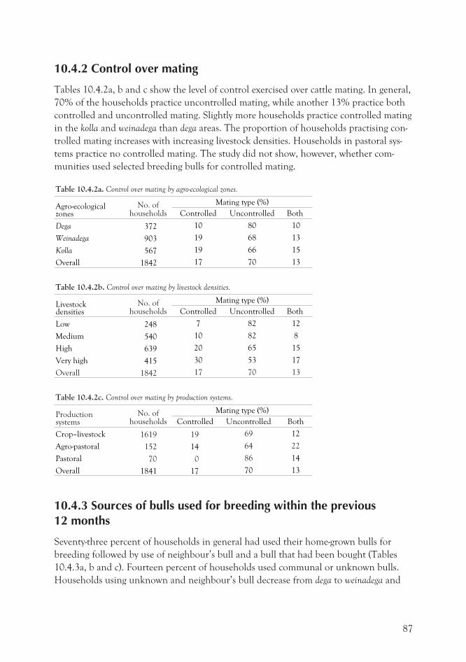
10.4.2 Control over mating
Tables 10.4.2a, b and c show the level of control exercised over cattle mating. In general,
70% of the households practice uncontrolled mating, while another 13% practice both
controlled and uncontrolled mating. Slightly more households practice controlled mating
in the kolla and weinadega than dega areas. The proportion of households practising con-
trolled mating increases with increasing livestock densities. Households in pastoral sys-
tems practice no controlled mating. The study did not show, however, whether com-
munities used selected breeding bulls for controlled mating.
Table 10.4.2a. Control over mating by agro-ecological zones.
Agro-ecologicalzones
No. ofhouseholds
Mating type (%)
Controlled Uncontrolled Both
Dega 372 10 80 10
Weinadega 903 19 68 13
Kolla 567 19 66 15
Overall 1842 17 70 13
Table 10.4.2b. Control over mating by livestock densities.
Livestockdensities
No. ofhouseholds
Mating type (%)
Controlled Uncontrolled Both
Low 248 7 82 12
Medium 540 10 82 8
High 639 20 65 15
Very high 415 30 53 17
Overall 1842 17 70 13
Table 10.4.2c. Control over mating by production systems.
Productionsystems
No. ofhouseholds
Mating type (%)
Controlled Uncontrolled Both
Crop–livestock 1619 19 69 12
Agro-pastoral 152 14 64 22
Pastoral 70 0 86 14
Overall 1841 17 70 13
10.4.3 Sources of bulls used for breeding within the previous12 months
Seventy-three percent of households in general had used their home-grown bulls for
breeding followed by use of neighbour’s bull and a bull that had been bought (Tables
10.4.3a, b and c). Fourteen percent of households used communal or unknown bulls.
Households using unknown and neighbour’s bull decrease from dega to weinadega and
87
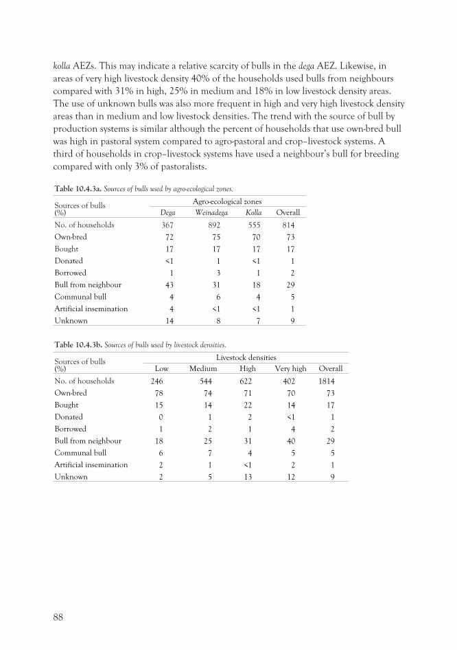
kolla AEZs. This may indicate a relative scarcity of bulls in the dega AEZ. Likewise, in
areas of very high livestock density 40% of the households used bulls from neighbours
compared with 31% in high, 25% in medium and 18% in low livestock density areas.
The use of unknown bulls was also more frequent in high and very high livestock density
areas than in medium and low livestock densities. The trend with the source of bull by
production systems is similar although the percent of households that use own-bred bull
was high in pastoral system compared to agro-pastoral and crop–livestock systems. A
third of households in crop–livestock systems have used a neighbour’s bull for breeding
compared with only 3% of pastoralists.
Table 10.4.3a. Sources of bulls used by agro-ecological zones.
Sources of bulls(%)
Agro-ecological zones
Dega Weinadega Kolla Overall
No. of households 367 892 555 814
Own-bred 72 75 70 73
Bought 17 17 17 17
Donated <1 1 <1 1
Borrowed 1 3 1 2
Bull from neighbour 43 31 18 29
Communal bull 4 6 4 5
Artificial insemination 4 <1 <1 1
Unknown 14 8 7 9
Table 10.4.3b. Sources of bulls used by livestock densities.
Sources of bulls(%)
Livestock densities
Low Medium High Very high Overall
No. of households 246 544 622 402 1814
Own-bred 78 74 71 70 73
Bought 15 14 22 14 17
Donated 0 1 2 <1 1
Borrowed 1 2 1 4 2
Bull from neighbour 18 25 31 40 29
Communal bull 6 7 4 5 5
Artificial insemination 2 1 <1 2 1
Unknown 2 5 13 12 9
88
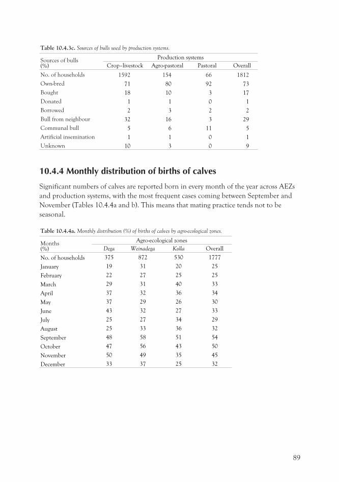
Table 10.4.3c. Sources of bulls used by production systems.
Sources of bulls(%)
Production systems
Crop–livestock Agro-pastoral Pastoral Overall
No. of households 1592 154 66 1812
Own-bred 71 80 92 73
Bought 18 10 3 17
Donated 1 1 0 1
Borrowed 2 3 2 2
Bull from neighbour 32 16 3 29
Communal bull 5 6 11 5
Artificial insemination 1 1 0 1
Unknown 10 3 0 9
10.4.4 Monthly distribution of births of calves
Significant numbers of calves are reported born in every month of the year across AEZs
and production systems, with the most frequent cases coming between September and
November (Tables 10.4.4a and b). This means that mating practice tends not to be
seasonal.
Table 10.4.4a. Monthly distribution (%) of births of calves by agro-ecological zones.
Months(%)
Agro-ecological zones
Dega Weinadega Kolla Overall
No. of households 375 872 530 1777
January 19 31 20 25
February 22 27 25 25
March 29 31 40 33
April 37 32 36 34
May 37 29 26 30
June 43 32 27 33
July 25 27 34 29
August 25 33 36 32
September 48 58 51 54
October 47 56 43 50
November 50 49 35 45
December 33 37 25 32
89
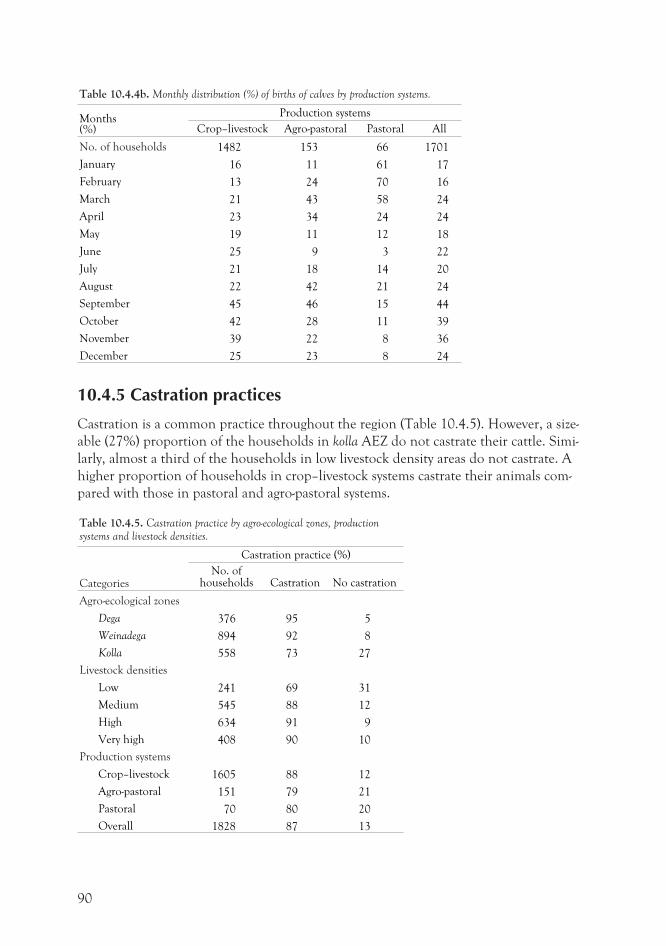
Table 10.4.4b. Monthly distribution (%) of births of calves by production systems.
Months(%)
Production systems
Crop–livestock Agro-pastoral Pastoral All
No. of households 1482 153 66 1701
January 16 11 61 17
February 13 24 70 16
March 21 43 58 24
April 23 34 24 24
May 19 11 12 18
June 25 9 3 22
July 21 18 14 20
August 22 42 21 24
September 45 46 15 44
October 42 28 11 39
November 39 22 8 36
December 25 23 8 24
10.4.5 Castration practices
Castration is a common practice throughout the region (Table 10.4.5). However, a size-
able (27%) proportion of the households in kolla AEZ do not castrate their cattle. Simi-
larly, almost a third of the households in low livestock density areas do not castrate. A
higher proportion of households in crop–livestock systems castrate their animals com-
pared with those in pastoral and agro-pastoral systems.
Table 10.4.5. Castration practice by agro-ecological zones, productionsystems and livestock densities.
Categories
Castration practice (%)
No. ofhouseholds Castration No castration
Agro-ecological zones
Dega 376 95 5
Weinadega 894 92 8
Kolla 558 73 27
Livestock densities
Low 241 69 31
Medium 545 88 12
High 634 91 9
Very high 408 90 10
Production systems
Crop–livestock 1605 88 12
Agro-pastoral 151 79 21
Pastoral 70 80 20
Overall 1828 87 13
90
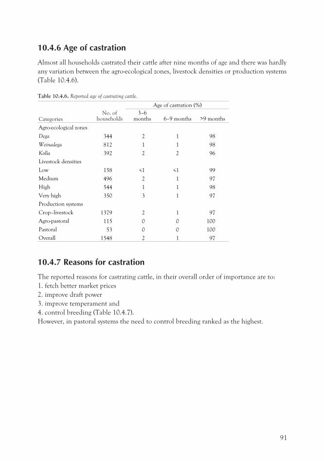
10.4.6 Age of castration
Almost all households castrated their cattle after nine months of age and there was hardly
any variation between the agro-ecological zones, livestock densities or production systems
(Table 10.4.6).
Table 10.4.6. Reported age of castrating cattle.
CategoriesNo. of
households
Age of castration (%)
3–6months 6–9 months >9 months
Agro-ecological zones
Dega 344 2 1 98
Weinadega 812 1 1 98
Kolla 392 2 2 96
Livestock densities
Low 158 <1 <1 99
Medium 496 2 1 97
High 544 1 1 98
Very high 350 3 1 97
Production systems
Crop–livestock 1379 2 1 97
Agro-pastoral 115 0 0 100
Pastoral 53 0 0 100
Overall 1548 2 1 97
10.4.7 Reasons for castration
The reported reasons for castrating cattle, in their overall order of importance are to:
1. fetch better market prices
2. improve draft power
3. improve temperament and
4. control breeding (Table 10.4.7).
However, in pastoral systems the need to control breeding ranked as the highest.
91
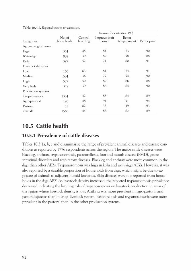
Table 10.4.7. Reported reasons for castration.
CategoriesNo. of
households
Reason for castration (%)
Controlbreeding
Improve draftpower
Bettertemperament Better price
Agro-ecological zones
Dega 354 45 84 73 90
Weinadega 807 39 89 58 88
Kolla 399 52 71 60 91
Livestock densities
Low 160 63 81 74 91
Medium 504 36 77 54 90
High 539 50 89 66 88
Very high 357 39 86 64 90
Production systems
Crop–livestock 1384 42 85 64 89
Agro-pastoral 120 48 91 51 94
Pastoral 55 82 33 49 93
Overall 1560 44 83 62 89
10.5 Cattle health
10.5.1 Prevalence of cattle diseases
Tables 10.5.1a, b, c and d summarise the range of prevalent animal diseases and disease con-
ditions as reported by 1776 respondents across the region. The major cattle diseases were
blackleg, anthrax, trypanosomosis, pasteurellosis, foot-and-mouth disease (FMD), gastro-
intestinal disorders and respiratory diseases. Blackleg and anthrax were more common in the
dega than other AEZs. Trypanosomosis was high in kolla and weinadega AEZs. However, it was
also reported by a sizeable proportion of households from dega, which might be due to ex-
posure of animals to adjacent humid lowlands. Skin diseases were not reported from house-
holds in the dega AEZ. As livestock density increased, the reported trypanosomosis prevalence
decreased indicating the limiting role of trypanosomosis on livestock production in areas of
the region where livestock density is low. Anthrax was more prevalent in agro-pastoral and
pastoral systems than in crop–livestock system. Pasteurellosis and trypanosomosis were more
prevalent in the pastoral than in the other production systems.
92
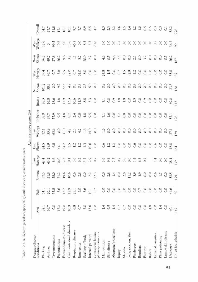
93
Tab
le10.5
.1a.
Rep
orte
dpr
evale
nce
(per
cent)
ofca
ttle
dise
ase
sby
adm
inis
trati
vezo
nes
.
Dis
ease
s/d
isea
seco
nd
itio
ns
Ad
min
istr
ativ
ezo
nes
(%)
Ove
rall
Ars
iB
ale
Bo
ran
aE
ast
Har
arge
Eas
tS
hew
aE
ast
Wel
lega
Illu
bab
or
Jim
ma
No
rth
Sh
ewa
Wes
tH
arar
geW
est
Sh
ewa
Wes
tW
elle
ga
Bla
ckle
g87.1
51.1
57.5
42.4
74.5
72.1
38.9
28.3
101.7
39.4
56.7
17.6
54.7
An
thra
x36.7
20.1
31.8
43.2
78.9
55.8
39.7
16.8
38.3
46.7
49.7
037.7
Try
pan
oso
mo
sis
0.0
33.8
38.0
8.6
6.8
63.6
57.9
18.6
0.0
0.7
27.8
99.5
31.8
Pas
teu
rell
osi
s12.2
3.6
21.2
36
.044.1
0.0
9.5
1.8
9.2
5.8
26.2
19.6
17.1
Fo
ot-an
d-m
ou
thd
isea
se19.0
13.7
19.6
12.2
34.2
31
.04.8
15.9
22.5
9.5
9.6
5.0
16.1
Gas
tro
-inte
stin
ald
iso
rder
s10.9
12.9
10.6
10.1
2.5
4.7
8.7
13.3
4.2
27
.03.7
13.6
10.1
Res
pir
ato
ryd
isea
ses
6.8
28.1
0.6
3.6
1.2
2.3
2.4
10.6
0.8
0.7
1.1
46.7
9.7
Em
erge
ncy
0.7
5.0
2.8
6.5
1.2
4.7
0.8
11.5
0.8
62.0
3.7
0.0
7.7
Sw
elli
ng
of
bo
dy
2.0
3.6
0.0
13.7
4.3
1.6
4.8
8.8
2.5
8.0
20.9
8.5
6.9
Inte
rnal
par
asit
es15.6
10.1
2.2
2.9
10.6
14
.09.5
5.3
5.0
0.0
2.7
3.5
6.5
Co
nta
gio
us
bo
vin
ep
leu
ro-p
neu
mo
nia
0.0
0.7
22.3
0.7
0.0
0.0
0.0
0.0
0.0
0.0
0.0
20.6
4.7
Mal
nu
trit
ion
1.4
0.0
0.0
3.6
0.6
1.6
7.1
7.1
0.8
24.8
4.3
3.0
4.3
Skin
dis
ease
9.5
0.0
2.8
9.4
1.2
0.0
1.6
0.0
0.0
1.5
0.5
1.0
2.3
Ab
ort
ion
/b
ruce
llo
sis
1.4
0.0
3.4
7.2
1.2
0.0
0.0
0.9
0.0
0.0
9.6
0.0
2.2
Inju
ry0.7
0.0
0.0
0.7
0.0
0.0
3.2
1.8
0.0
0.7
7.5
2.5
1.6
Mas
titi
s0.7
5.0
2.8
5.8
0.0
0.0
0.8
1.8
0.8
1.5
0.0
0.0
1.5
3-d
aysi
ckn
ess,
Buta
0.0
0.0
11.2
0.0
0.0
0.0
0.0
0.0
0.0
2.9
0.0
0.0
1.4
Rin
der
pes
t0.0
0.0
3.9
1.4
0.6
0.0
0.0
3.5
0.8
2.2
2.1
0.0
1.2
Bo
tuli
sm0.0
0.7
3.9
6.5
0.0
0.0
0.0
0.0
0.0
0.0
0.0
0.0
1.0
Fo
ot
rot
0.0
0.0
0.0
0.7
0.0
0.0
0.0
0.9
0.0
0.0
3.2
0.0
0.5
Rab
ies
4.8
0.0
0.0
0.0
0.0
0.0
0.0
0.8
0.0
0.0
0.0
0.5
Ext
ern
alp
aras
ites
0.0
0.0
0.6
1.4
0.6
0.0
0.0
0.0
0.0
0.0
0.0
0.5
0.3
Pla
nt
po
iso
nin
g1.4
0.0
1.7
0.0
0.0
0.0
0.0
0.0
0.0
0.0
0.0
0.0
0.3
Lu
mp
ysk
ind
isea
se0.0
0.0
0.0
0.0
0.0
0.0
0.0
0.0
0.0
0.0
0.5
0.0
0.1
Un
kn
ow
n40.1
44.6
52.5
38.1
16.8
27.1
57.1
69
.023.3
35.8
26.2
36.2
38.2
No
.o
fh
ou
seh
old
s147
139
179
139
161
129
126
113
120
137
187
199
1776
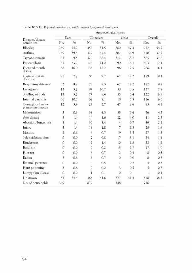
Table 10.5.1b. Reported prevalence of cattle diseases by agro-ecological zones.
Diseases/diseaseconditions
Agro-ecological zones
Dega Weinadega Kolla Overall
No. % No. % No. % No. %
Blackleg 259 74.2 453 51.5 260 47.4 972 54.7
Anthrax 139 39.8 329 37.4 202 36.9 670 37.7
Trypanosomosis 33 9.5 320 36.4 212 38.7 565 31.8
Pasteurellosis 81 23.2 123 14.0 99 18.1 303 17.1
Foot-and-mouthdisease
56 16.0 134 15.2 96 17.5 286 16.1
Gastro-intestinaldisorder
27 7.7 85 9.7 67 12.2 179 10.1
Respiratory diseases 32 9.2 73 8.3 67 12.2 172 9.7
Emergency 13 3.7 94 10.7 30 5.5 137 7.7
Swelling of body 13 3.7 74 8.4 35 6.4 122 6.9
Internal parasites 36 10.3 62 7.1 18 3.3 116 6.5
Contagious bovinepleuro-pneumonia
12 3.4 24 2.7 47 8.6 83 4.7
Malnutrition 3 0.9 38 4.3 35 6.4 76 4.3
Skin disease 5 1.4 14 1.6 22 4.0 41 2.3
Abortion/brucellosis 5 1.4 30 3.4 4 0.7 39 2.2
Injury 5 1.4 16 1.8 7 1.3 28 1.6
Mastitis 2 0.6 6 0.7 19 3.5 27 1.5
3-day sickness, Buta 0 0.0 7 0.8 17 3.1 24 1.4
Rinderpest 0 0.0 12 1.4 10 1.8 22 1.2
Botulism 0 0.0 2 0.2 15 2.7 17 1.0
Foot rot 0 0.0 6 0.7 2 0.4 8 0.5
Rabies 2 0.6 6 0.7 0 0.0 8 0.5
External parasites 0 0.0 4 0.5 1 0.2 5 0.3
Plant poisoning 2 0.6 0 0.0 3 0.5 5 0.3
Lumpy skin disease 0 0.0 1 0.1 0 0 1 0.1
Unknown 85 24.4 366 41.6 227 41.4 678 38.2
No. of households 349 879 548 1776
94
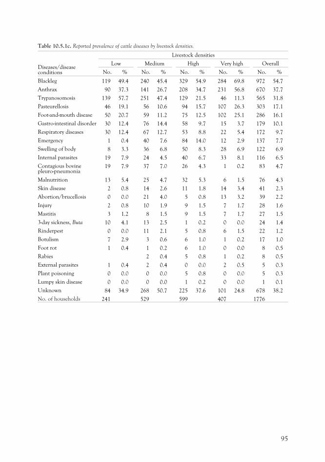
Table 10.5.1c. Reported prevalence of cattle diseases by livestock densities.
Diseases/diseaseconditions
Livestock densities
Low Medium High Very high Overall
No. % No. % No. % No. % No. %
Blackleg 119 49.4 240 45.4 329 54.9 284 69.8 972 54.7
Anthrax 90 37.3 141 26.7 208 34.7 231 56.8 670 37.7
Trypanosomosis 139 57.7 251 47.4 129 21.5 46 11.3 565 31.8
Pasteurellosis 46 19.1 56 10.6 94 15.7 107 26.3 303 17.1
Foot-and-mouth disease 50 20.7 59 11.2 75 12.5 102 25.1 286 16.1
Gastro-intestinal disorder 30 12.4 76 14.4 58 9.7 15 3.7 179 10.1
Respiratory diseases 30 12.4 67 12.7 53 8.8 22 5.4 172 9.7
Emergency 1 0.4 40 7.6 84 14.0 12 2.9 137 7.7
Swelling of body 8 3.3 36 6.8 50 8.3 28 6.9 122 6.9
Internal parasites 19 7.9 24 4.5 40 6.7 33 8.1 116 6.5
Contagious bovinepleuro-pneumonia
19 7.9 37 7.0 26 4.3 1 0.2 83 4.7
Malnutrition 13 5.4 25 4.7 32 5.3 6 1.5 76 4.3
Skin disease 2 0.8 14 2.6 11 1.8 14 3.4 41 2.3
Abortion/brucellosis 0 0.0 21 4.0 5 0.8 13 3.2 39 2.2
Injury 2 0.8 10 1.9 9 1.5 7 1.7 28 1.6
Mastitis 3 1.2 8 1.5 9 1.5 7 1.7 27 1.5
3-day sickness, Buta 10 4.1 13 2.5 1 0.2 0 0.0 24 1.4
Rinderpest 0 0.0 11 2.1 5 0.8 6 1.5 22 1.2
Botulism 7 2.9 3 0.6 6 1.0 1 0.2 17 1.0
Foot rot 1 0.4 1 0.2 6 1.0 0 0.0 8 0.5
Rabies 2 0.4 5 0.8 1 0.2 8 0.5
External parasites 1 0.4 2 0.4 0 0.0 2 0.5 5 0.3
Plant poisoning 0 0.0 0 0.0 5 0.8 0 0.0 5 0.3
Lumpy skin disease 0 0.0 0 0.0 1 0.2 0 0.0 1 0.1
Unknown 84 34.9 268 50.7 225 37.6 101 24.8 678 38.2
No. of households 241 529 599 407 1776
95
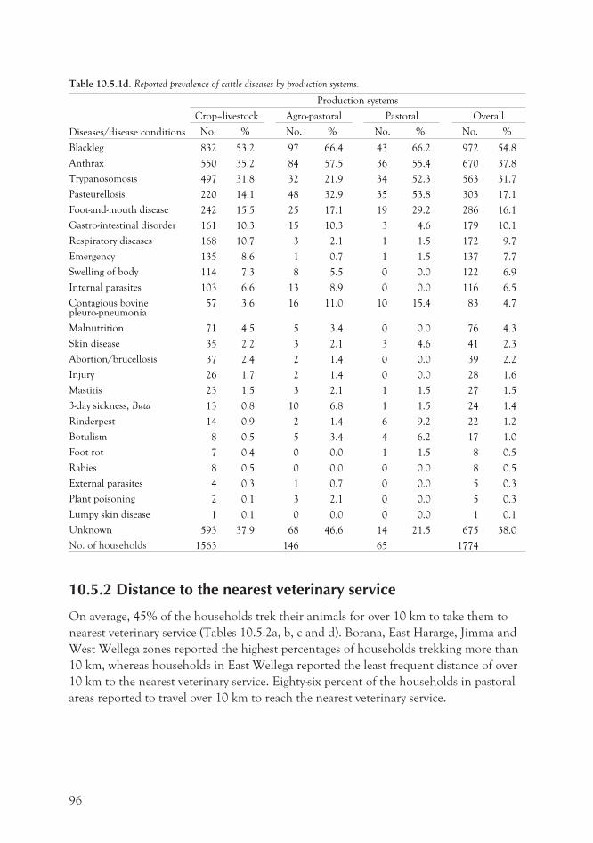
Table 10.5.1d. Reported prevalence of cattle diseases by production systems.
Diseases/disease conditions
Production systems
Crop–livestock Agro-pastoral Pastoral Overall
No. % No. % No. % No. %
Blackleg 832 53.2 97 66.4 43 66.2 972 54.8
Anthrax 550 35.2 84 57.5 36 55.4 670 37.8
Trypanosomosis 497 31.8 32 21.9 34 52.3 563 31.7
Pasteurellosis 220 14.1 48 32.9 35 53.8 303 17.1
Foot-and-mouth disease 242 15.5 25 17.1 19 29.2 286 16.1
Gastro-intestinal disorder 161 10.3 15 10.3 3 4.6 179 10.1
Respiratory diseases 168 10.7 3 2.1 1 1.5 172 9.7
Emergency 135 8.6 1 0.7 1 1.5 137 7.7
Swelling of body 114 7.3 8 5.5 0 0.0 122 6.9
Internal parasites 103 6.6 13 8.9 0 0.0 116 6.5
Contagious bovinepleuro-pneumonia
57 3.6 16 11.0 10 15.4 83 4.7
Malnutrition 71 4.5 5 3.4 0 0.0 76 4.3
Skin disease 35 2.2 3 2.1 3 4.6 41 2.3
Abortion/brucellosis 37 2.4 2 1.4 0 0.0 39 2.2
Injury 26 1.7 2 1.4 0 0.0 28 1.6
Mastitis 23 1.5 3 2.1 1 1.5 27 1.5
3-day sickness, Buta 13 0.8 10 6.8 1 1.5 24 1.4
Rinderpest 14 0.9 2 1.4 6 9.2 22 1.2
Botulism 8 0.5 5 3.4 4 6.2 17 1.0
Foot rot 7 0.4 0 0.0 1 1.5 8 0.5
Rabies 8 0.5 0 0.0 0 0.0 8 0.5
External parasites 4 0.3 1 0.7 0 0.0 5 0.3
Plant poisoning 2 0.1 3 2.1 0 0.0 5 0.3
Lumpy skin disease 1 0.1 0 0.0 0 0.0 1 0.1
Unknown 593 37.9 68 46.6 14 21.5 675 38.0
No. of households 1563 146 65 1774
10.5.2 Distance to the nearest veterinary service
On average, 45% of the households trek their animals for over 10 km to take them to
nearest veterinary service (Tables 10.5.2a, b, c and d). Borana, East Hararge, Jimma and
West Wellega zones reported the highest percentages of households trekking more than
10 km, whereas households in East Wellega reported the least frequent distance of over
10 km to the nearest veterinary service. Eighty-six percent of the households in pastoral
areas reported to travel over 10 km to reach the nearest veterinary service.
96
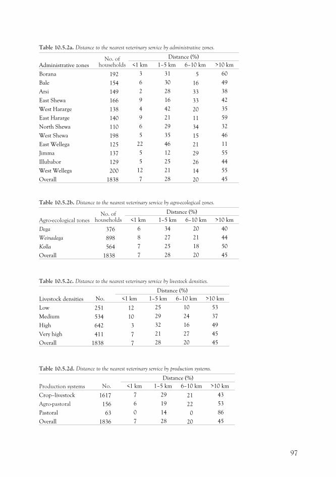
Table 10.5.2a. Distance to the nearest veterinary service by administrative zones.
Administrative zonesNo. of
households
Distance (%)
<1 km 1–5 km 6–10 km >10 km
Borana 192 3 31 5 60
Bale 154 6 30 16 49
Arsi 149 2 28 33 38
East Shewa 166 9 16 33 42
West Hararge 138 4 42 20 35
East Hararge 140 9 21 11 59
North Shewa 110 6 29 34 32
West Shewa 198 5 35 15 46
East Wellega 125 22 46 21 11
Jimma 137 5 12 29 55
Illubabor 129 5 25 26 44
West Wellega 200 12 21 14 55
Overall 1838 7 28 20 45
Table 10.5.2b. Distance to the nearest veterinary service by agro-ecological zones.
Agro-ecological zonesNo. of
households
Distance (%)
<1 km 1–5 km 6–10 km >10 km
Dega 376 6 34 20 40
Weinadega 898 8 27 21 44
Kolla 564 7 25 18 50
Overall 1838 7 28 20 45
Table 10.5.2c. Distance to the nearest veterinary service by livestock densities.
Livestock densities No.
Distance (%)
<1 km 1–5 km 6–10 km >10 km
Low 251 12 25 10 53
Medium 534 10 29 24 37
High 642 3 32 16 49
Very high 411 7 21 27 45
Overall 1838 7 28 20 45
Table 10.5.2d. Distance to the nearest veterinary service by production systems.
Production systems No.
Distance (%)
<1 km 1–5 km 6–10 km >10 km
Crop–livestock 1617 7 29 21 43
Agro-pastoral 156 6 19 22 53
Pastoral 63 0 14 0 86
Overall 1836 7 28 20 45
97
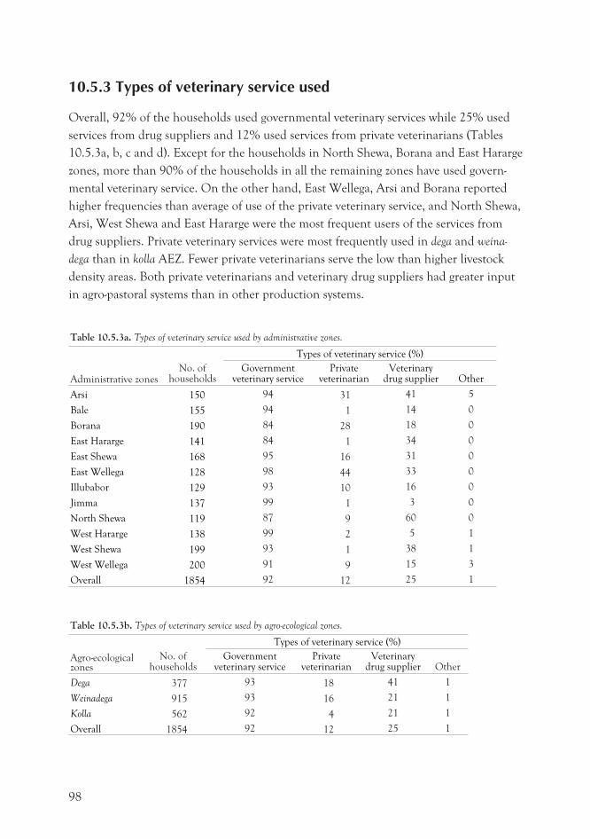
10.5.3 Types of veterinary service used
Overall, 92% of the households used governmental veterinary services while 25% used
services from drug suppliers and 12% used services from private veterinarians (Tables
10.5.3a, b, c and d). Except for the households in North Shewa, Borana and East Hararge
zones, more than 90% of the households in all the remaining zones have used govern-
mental veterinary service. On the other hand, East Wellega, Arsi and Borana reported
higher frequencies than average of use of the private veterinary service, and North Shewa,
Arsi, West Shewa and East Hararge were the most frequent users of the services from
drug suppliers. Private veterinary services were most frequently used in dega and weina-
dega than in kolla AEZ. Fewer private veterinarians serve the low than higher livestock
density areas. Both private veterinarians and veterinary drug suppliers had greater input
in agro-pastoral systems than in other production systems.
Table 10.5.3a. Types of veterinary service used by administrative zones.
Administrative zonesNo. of
households
Types of veterinary service (%)
Governmentveterinary service
Privateveterinarian
Veterinarydrug supplier Other
Arsi 150 94 31 41 5
Bale 155 94 1 14 0
Borana 190 84 28 18 0
East Hararge 141 84 1 34 0
East Shewa 168 95 16 31 0
East Wellega 128 98 44 33 0
Illubabor 129 93 10 16 0
Jimma 137 99 1 3 0
North Shewa 119 87 9 60 0
West Hararge 138 99 2 5 1
West Shewa 199 93 1 38 1
West Wellega 200 91 9 15 3
Overall 1854 92 12 25 1
Table 10.5.3b. Types of veterinary service used by agro-ecological zones.
Agro-ecologicalzones
No. ofhouseholds
Types of veterinary service (%)
Governmentveterinary service
Privateveterinarian
Veterinarydrug supplier Other
Dega 377 93 18 41 1
Weinadega 915 93 16 21 1
Kolla 562 92 4 21 1
Overall 1854 92 12 25 1
98
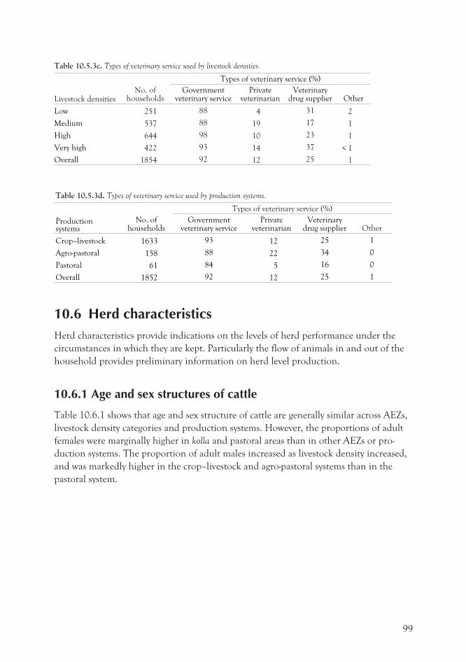
Table 10.5.3c. Types of veterinary service used by livestock densities.
Livestock densitiesNo. of
households
Types of veterinary service (%)
Governmentveterinary service
Privateveterinarian
Veterinarydrug supplier Other
Low 251 88 4 31 2
Medium 537 88 19 17 1
High 644 98 10 23 1
Very high 422 93 14 37 < 1
Overall 1854 92 12 25 1
Table 10.5.3d. Types of veterinary service used by production systems.
Productionsystems
No. ofhouseholds
Types of veterinary service (%)
Governmentveterinary service
Privateveterinarian
Veterinarydrug supplier Other
Crop–livestock 1633 93 12 25 1
Agro-pastoral 158 88 22 34 0
Pastoral 61 84 5 16 0
Overall 1852 92 12 25 1
10.6 Herd characteristicsHerd characteristics provide indications on the levels of herd performance under the
circumstances in which they are kept. Particularly the flow of animals in and out of the
household provides preliminary information on herd level production.
10.6.1 Age and sex structures of cattle
Table 10.6.1 shows that age and sex structure of cattle are generally similar across AEZs,
livestock density categories and production systems. However, the proportions of adult
females were marginally higher in kolla and pastoral areas than in other AEZs or pro-
duction systems. The proportion of adult males increased as livestock density increased,
and was markedly higher in the crop–livestock and agro-pastoral systems than in the
pastoral system.
99
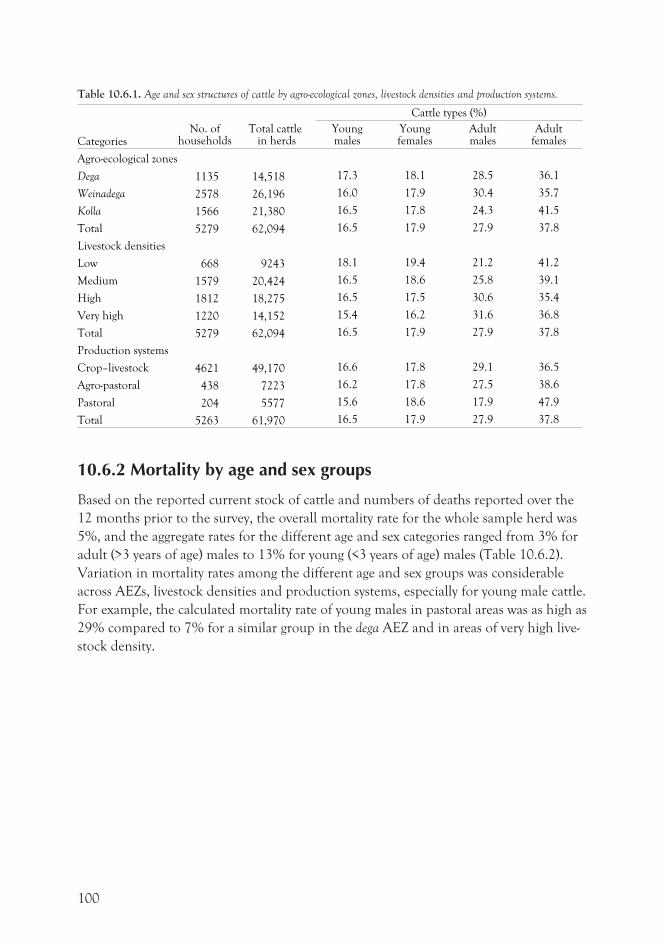
Table 10.6.1. Age and sex structures of cattle by agro-ecological zones, livestock densities and production systems.
CategoriesNo. of
householdsTotal cattle
in herds
Cattle types (%)
Youngmales
Youngfemales
Adultmales
Adultfemales
Agro-ecological zones
Dega 1135 14,518 17.3 18.1 28.5 36.1
Weinadega 2578 26,196 16.0 17.9 30.4 35.7
Kolla 1566 21,380 16.5 17.8 24.3 41.5
Total 5279 62,094 16.5 17.9 27.9 37.8
Livestock densities
Low 668 9243 18.1 19.4 21.2 41.2
Medium 1579 20,424 16.5 18.6 25.8 39.1
High 1812 18,275 16.5 17.5 30.6 35.4
Very high 1220 14,152 15.4 16.2 31.6 36.8
Total 5279 62,094 16.5 17.9 27.9 37.8
Production systems
Crop–livestock 4621 49,170 16.6 17.8 29.1 36.5
Agro-pastoral 438 7223 16.2 17.8 27.5 38.6
Pastoral 204 5577 15.6 18.6 17.9 47.9
Total 5263 61,970 16.5 17.9 27.9 37.8
10.6.2 Mortality by age and sex groups
Based on the reported current stock of cattle and numbers of deaths reported over the
12 months prior to the survey, the overall mortality rate for the whole sample herd was
5%, and the aggregate rates for the different age and sex categories ranged from 3% for
adult (>3 years of age) males to 13% for young (<3 years of age) males (Table 10.6.2).
Variation in mortality rates among the different age and sex groups was considerable
across AEZs, livestock densities and production systems, especially for young male cattle.
For example, the calculated mortality rate of young males in pastoral areas was as high as
29% compared to 7% for a similar group in the dega AEZ and in areas of very high live-
stock density.
100
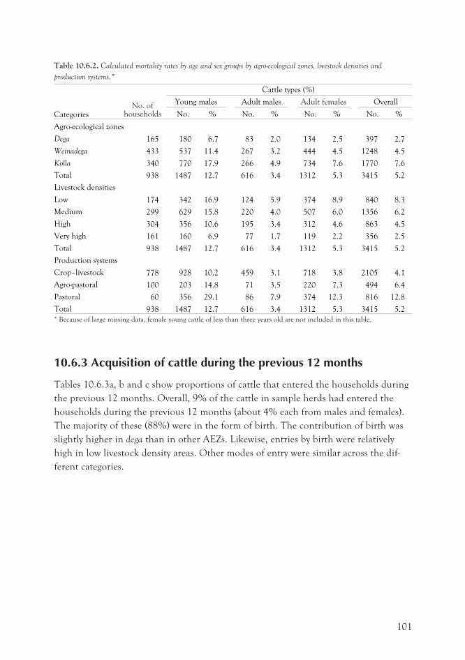
Table 10.6.2. Calculated mortality rates by age and sex groups by agro-ecological zones, livestock densities and
production systems.*
CategoriesNo. of
households
Cattle types (%)
Young males Adult males Adult females Overall
No. % No. % No. % No. %
Agro-ecological zones
Dega 165 180 6.7 83 2.0 134 2.5 397 2.7
Weinadega 433 537 11.4 267 3.2 444 4.5 1248 4.5
Kolla 340 770 17.9 266 4.9 734 7.6 1770 7.6
Total 938 1487 12.7 616 3.4 1312 5.3 3415 5.2
Livestock densities
Low 174 342 16.9 124 5.9 374 8.9 840 8.3
Medium 299 629 15.8 220 4.0 507 6.0 1356 6.2
High 304 356 10.6 195 3.4 312 4.6 863 4.5
Very high 161 160 6.9 77 1.7 119 2.2 356 2.5
Total 938 1487 12.7 616 3.4 1312 5.3 3415 5.2
Production systems
Crop–livestock 778 928 10.2 459 3.1 718 3.8 2105 4.1
Agro-pastoral 100 203 14.8 71 3.5 220 7.3 494 6.4
Pastoral 60 356 29.1 86 7.9 374 12.3 816 12.8
Total 938 1487 12.7 616 3.4 1312 5.3 3415 5.2
* Because of large missing data, female young cattle of less than three years old are not included in this table.
10.6.3 Acquisition of cattle during the previous 12 months
Tables 10.6.3a, b and c show proportions of cattle that entered the households during
the previous 12 months. Overall, 9% of the cattle in sample herds had entered the
households during the previous 12 months (about 4% each from males and females).
The majority of these (88%) were in the form of birth. The contribution of birth was
slightly higher in dega than in other AEZs. Likewise, entries by birth were relatively
high in low livestock density areas. Other modes of entry were similar across the dif-
ferent categories.
101
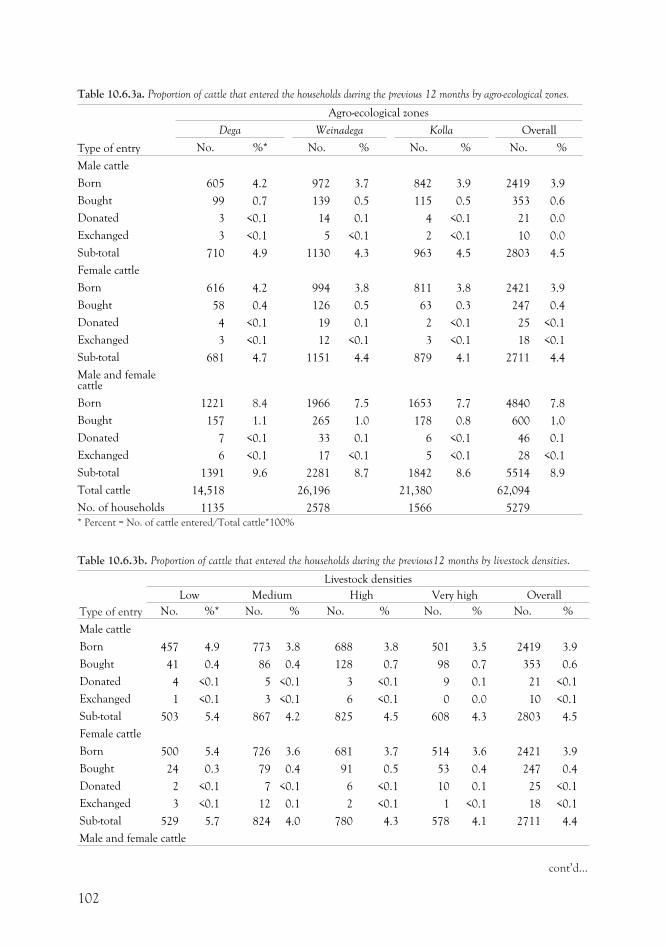
Table 10.6.3a. Proportion of cattle that entered the households during the previous 12 months by agro-ecological zones.
Type of entry
Agro-ecological zones
Dega Weinadega Kolla Overall
No. %* No. % No. % No. %
Male cattle
Born 605 4.2 972 3.7 842 3.9 2419 3.9
Bought 99 0.7 139 0.5 115 0.5 353 0.6
Donated 3 <0.1 14 0.1 4 <0.1 21 0.0
Exchanged 3 <0.1 5 <0.1 2 <0.1 10 0.0
Sub-total 710 4.9 1130 4.3 963 4.5 2803 4.5
Female cattle
Born 616 4.2 994 3.8 811 3.8 2421 3.9
Bought 58 0.4 126 0.5 63 0.3 247 0.4
Donated 4 <0.1 19 0.1 2 <0.1 25 <0.1
Exchanged 3 <0.1 12 <0.1 3 <0.1 18 <0.1
Sub-total 681 4.7 1151 4.4 879 4.1 2711 4.4
Male and femalecattle
Born 1221 8.4 1966 7.5 1653 7.7 4840 7.8
Bought 157 1.1 265 1.0 178 0.8 600 1.0
Donated 7 <0.1 33 0.1 6 <0.1 46 0.1
Exchanged 6 <0.1 17 <0.1 5 <0.1 28 <0.1
Sub-total 1391 9.6 2281 8.7 1842 8.6 5514 8.9
Total cattle 14,518 26,196 21,380 62,094
No. of households 1135 2578 1566 5279
* Percent = No. of cattle entered/Total cattle*100%
Table 10.6.3b. Proportion of cattle that entered the households during the previous12 months by livestock densities.
Type of entry
Livestock densities
Low Medium High Very high Overall
No. %* No. % No. % No. % No. %
Male cattle
Born 457 4.9 773 3.8 688 3.8 501 3.5 2419 3.9
Bought 41 0.4 86 0.4 128 0.7 98 0.7 353 0.6
Donated 4 <0.1 5 <0.1 3 <0.1 9 0.1 21 <0.1
Exchanged 1 <0.1 3 <0.1 6 <0.1 0 0.0 10 <0.1
Sub-total 503 5.4 867 4.2 825 4.5 608 4.3 2803 4.5
Female cattle
Born 500 5.4 726 3.6 681 3.7 514 3.6 2421 3.9
Bought 24 0.3 79 0.4 91 0.5 53 0.4 247 0.4
Donated 2 <0.1 7 <0.1 6 <0.1 10 0.1 25 <0.1
Exchanged 3 <0.1 12 0.1 2 <0.1 1 <0.1 18 <0.1
Sub-total 529 5.7 824 4.0 780 4.3 578 4.1 2711 4.4
Male and female cattle
102
cont’d...
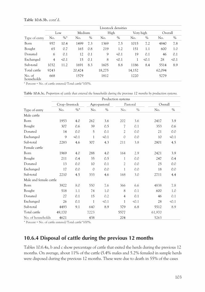
Type of entry
Livestock densities
Low Medium High Very high Overall
No. %* No. % No. % No. % No. %
Born 957 10.4 1499 7.3 1369 7.5 1015 7.2 4840 7.8
Bought 65 0.7 165 0.8 219 1.2 151 1.1 600 1.0
Donated 6 0.1 12 0.1 9 <0.1 19 0.1 46 0.1
Exchanged 4 <0.1 15 0.1 8 <0.1 1 <0.1 28 <0.1
Sub-total 1032 11.2 1691 8.3 1605 8.8 1186 8.4 5514 8.9
Total cattle 9243 20,424 18,275 14,152 62,094
No. ofhouseholds
668 1579 1812 1220 5279
* Percent = No. of cattle entered/Total cattle*100%.
Table 10.6.3c. Proportion of cattle that entered the households during the previous 12 months by production systems.
Type of entry
Production systems
Crop–livestock Agro-pastoral Pastoral Overall
No. %* No. % No. % No. %
Male cattle
Born 1953 4.0 262 3.6 202 3.6 2417 3.9
Bought 307 0.6 39 0.5 7 0.1 353 0.6
Donated 14 0.0 5 0.1 2 0.0 21 0.0
Exchanged 9 <0.1 1 <0.1 0 0.0 10 <0.1
Sub-total 2283 4.6 307 4.3 211 3.8 2801 4.5
Female cattle
Born 1969 4.0 288 4.0 164 2.9 2421 3.9
Bought 211 0.4 35 0.5 1 0.0 247 0.4
Donated 13 0.0 10 0.1 2 0.0 25 0.0
Exchanged 17 0.0 0 0.0 1 0.0 18 0.0
Sub-total 2210 4.5 333 4.6 168 3.0 2711 4.4
Male and female cattle
Born 3922 8.0 550 7.6 366 6.6 4838 7.8
Bought 518 1.1 74 1.0 8 0.1 600 1.0
Donated 27 0.1 15 0.2 4 0.1 46 0.1
Exchanged 26 0.1 1 <0.1 1 <0.1 28 <0.1
Sub-total 4493 9.1 640 8.9 379 6.8 5512 8.9
Total cattle 49,170 7223 5577 61,970
No. of households 4621 438 204 5263
* Percent = No. of cattle entered/Total cattle*100%.
10.6.4 Disposal of cattle during the previous 12 months
Tables 10.6.4a, b and c show percentage of cattle that exited the herds during the previous 12
months. On average, about 11% of the cattle (5.4% males and 5.2% females) in sample herds
were disposed during the previous 12 months. These were due to death in 55% of the cases
103
Table 10.6.3b. cont’d.
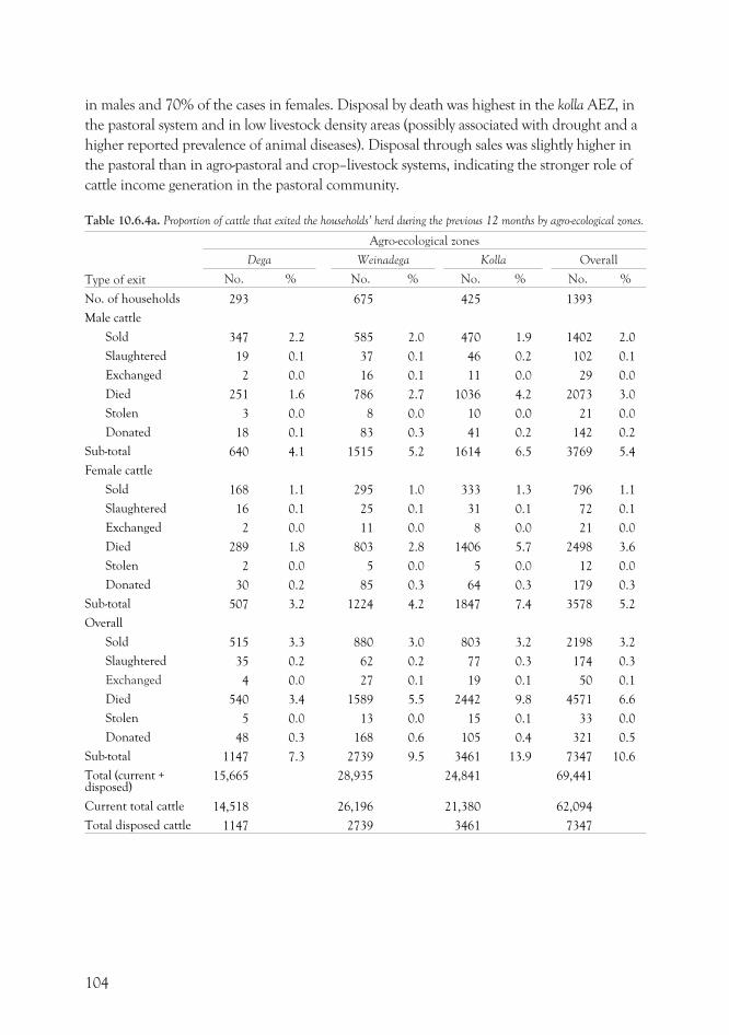
in males and 70% of the cases in females. Disposal by death was highest in the kolla AEZ, in
the pastoral system and in low livestock density areas (possibly associated with drought and a
higher reported prevalence of animal diseases). Disposal through sales was slightly higher in
the pastoral than in agro-pastoral and crop–livestock systems, indicating the stronger role of
cattle income generation in the pastoral community.
Table 10.6.4a. Proportion of cattle that exited the households’ herd during the previous 12 months by agro-ecological zones.
Type of exit
Agro-ecological zones
Dega Weinadega Kolla Overall
No. % No. % No. % No. %
No. of households 293 675 425 1393
Male cattle
Sold 347 2.2 585 2.0 470 1.9 1402 2.0
Slaughtered 19 0.1 37 0.1 46 0.2 102 0.1
Exchanged 2 0.0 16 0.1 11 0.0 29 0.0
Died 251 1.6 786 2.7 1036 4.2 2073 3.0
Stolen 3 0.0 8 0.0 10 0.0 21 0.0
Donated 18 0.1 83 0.3 41 0.2 142 0.2
Sub-total 640 4.1 1515 5.2 1614 6.5 3769 5.4
Female cattle
Sold 168 1.1 295 1.0 333 1.3 796 1.1
Slaughtered 16 0.1 25 0.1 31 0.1 72 0.1
Exchanged 2 0.0 11 0.0 8 0.0 21 0.0
Died 289 1.8 803 2.8 1406 5.7 2498 3.6
Stolen 2 0.0 5 0.0 5 0.0 12 0.0
Donated 30 0.2 85 0.3 64 0.3 179 0.3
Sub-total 507 3.2 1224 4.2 1847 7.4 3578 5.2
Overall
Sold 515 3.3 880 3.0 803 3.2 2198 3.2
Slaughtered 35 0.2 62 0.2 77 0.3 174 0.3
Exchanged 4 0.0 27 0.1 19 0.1 50 0.1
Died 540 3.4 1589 5.5 2442 9.8 4571 6.6
Stolen 5 0.0 13 0.0 15 0.1 33 0.0
Donated 48 0.3 168 0.6 105 0.4 321 0.5
Sub-total 1147 7.3 2739 9.5 3461 13.9 7347 10.6
Total (current +disposed)
15,665 28,935 24,841 69,441
Current total cattle 14,518 26,196 21,380 62,094
Total disposed cattle 1147 2739 3461 7347
104
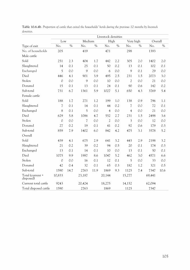
Table 10.6.4b. Proportion of cattle that exited the households’ herds during the previous 12 months by livestock
densities.
Type of exit
Livestock densities
Low Medium High Very high Overall
No. % No. % No. % No. % No. %
No. of households 205 419 471 298 1393
Male cattle
Sold 251 2.3 404 1.7 442 2.2 305 2.0 1402 2.0
Slaughtered 14 0.1 25 0.1 50 0.2 13 0.1 102 0.1
Exchanged 5 0.0 9 0.0 6 0.0 9 0.1 29 0.0
Died 446 4.1 901 3.9 495 2.5 231 1.5 2073 3.0
Stolen 0 0.0 9 0.0 10 0.0 2 0.0 21 0.0
Donated 15 0.1 13 0.1 24 0.1 90 0.6 142 0.2
Sub-total 731 6.7 1361 5.9 1027 5.1 650 4.3 3769 5.4
Female cattle
Sold 188 1.7 271 1.2 199 1.0 138 0.9 796 1.1
Slaughtered 7 0.1 14 0.1 44 0.2 7 0.0 72 0.1
Exchanged 8 0.1 5 0.0 4 0.0 4 0.0 21 0.0
Died 629 5.8 1086 4.7 552 2.7 231 1.5 2498 3.6
Stolen 0 0.0 7 0.0 2 0.0 3 0.0 12 0.0
Donated 27 0.2 19 0.1 41 0.2 92 0.6 179 0.3
Sub-total 859 7.9 1402 6.0 842 4.2 475 3.1 3578 5.2
Overall
Sold 439 4.1 675 2.9 641 3.2 443 2.9 2198 3.2
Slaughtered 21 0.2 39 0.2 94 0.5 20 0.1 174 0.3
Exchanged 13 0.1 14 0.1 10 0.0 13 0.1 50 0.1
Died 1075 9.9 1987 8.6 1047 5.2 462 3.0 4571 6.6
Stolen 0 0.0 16 0.1 12 0.1 5 0.0 33 0.0
Donated 42 0.4 32 0.1 65 0.3 182 1.2 321 0.5
Sub-total 1590 14.7 2763 11.9 1869 9.3 1125 7.4 7347 10.6
Total (current +disposed)
10,833 23,187 20,144 15,277 69,441
Current total cattle 9243 20,424 18,275 14,152 62,094
Total disposed cattle 1590 2763 1869 1125 7347
105
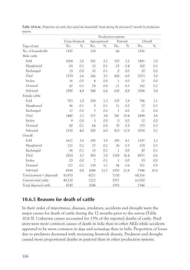
Table 10.6.4c. Proportion of cattle that exited the households’ herds during the previous12 months by production
systems.
Type of exit
Production systems
Crop–livestock Agro-pastoral Pastoral Overall
No. % No. % No. % No. %
No. of households 1197 129 66 1392
Male cattle
Sold 1064 2.0 182 2.2 155 2.2 1401 2.0
Slaughtered 65 0.1 12 0.1 25 0.4 102 0.1
Exchanged 19 0.0 10 0.1 0 0.0 29 0.0
Died 1379 2.6 266 3.2 428 6.0 2073 3.0
Stolen 16 0.0 4 0.0 1 0.0 21 0.0
Donated 47 0.1 74 0.9 21 0.3 142 0.2
Sub-total 2590 4.8 548 6.6 630 8.8 3768 5.4
Female cattle
Sold 553 1.0 108 1.3 135 1.9 796 1.1
Slaughtered 56 0.1 5 0.1 11 0.2 72 0.1
Exchanged 17 0.0 3 0.0 1 0.0 21 0.0
Died 1440 2.7 317 3.8 741 10.4 2498 3.6
Stolen 9 0.0 3 0.0 0 0.0 12 0.0
Donated 80 0.1 64 0.8 35 0.5 179 0.3
Sub-total 2155 4.0 500 6.0 923 12.9 3578 5.2
Overall
Sold 1617 3.0 290 3.5 290 4.1 2197 3.2
Slaughtered 121 0.2 17 0.2 36 0.5 174 0.3
Exchanged 36 0.1 13 0.2 1 0.0 50 0.1
Died 2819 5.2 583 7.0 1169 16.4 4571 6.6
Stolen 25 0.0 7 0.1 1 0.0 33 0.0
Donated 127 0.2 138 1.7 56 0.8 321 0.5
Sub-total 4745 8.8 1048 12.7 1553 21.8 7346 10.6
Total (current + disposed) 53,915 8271 7130 69,316
Current total cattle 49,170 7223 5577 61,970
Total disposed cattle 4745 1048 1553 7346
10.6.5 Reasons for death of cattle
In their order of importance, diseases, predators, accidents and drought were the
major causes for death of cattle during the 12 months prior to the survey (Table
10.6.5). Unknown causes accounted for 13% of the reported deaths of cattle. Pred-
ators were more common causes of death in kolla than in other AEZs while accidents
appeared to be more common in dega and weinadega than in kolla. Proportion of losses
due to predators decreased with increasing livestock density. Predators and drought
caused more proportional deaths in pastoral than in other production systems.
106
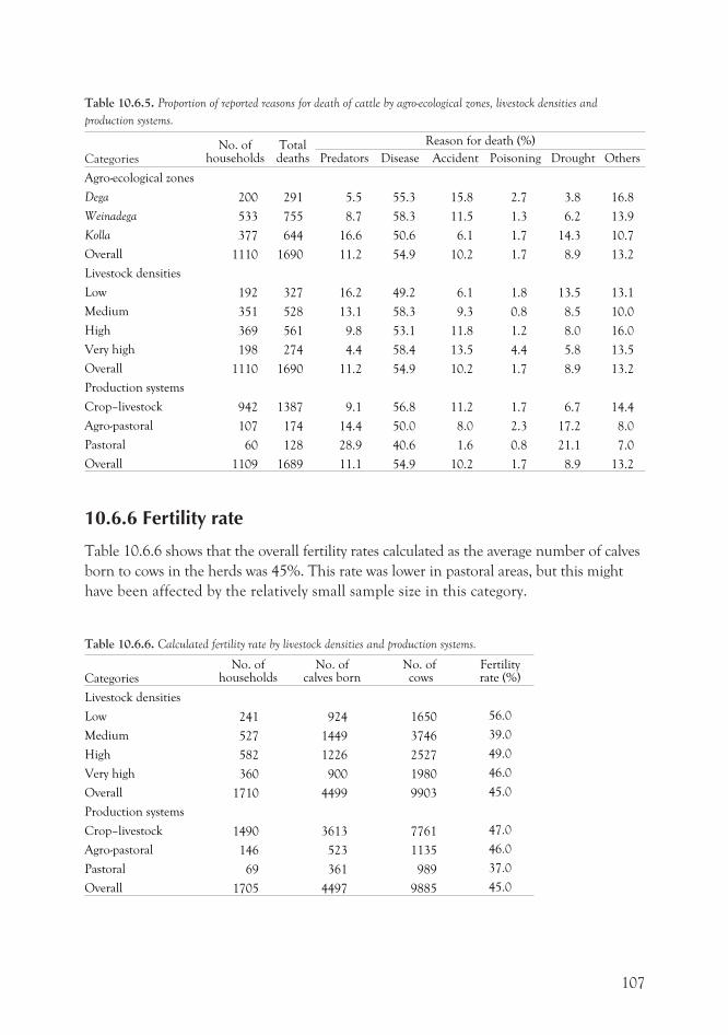
Table 10.6.5. Proportion of reported reasons for death of cattle by agro-ecological zones, livestock densities and
production systems.
CategoriesNo. of
householdsTotaldeaths
Reason for death (%)
Predators Disease Accident Poisoning Drought Others
Agro-ecological zones
Dega 200 291 5.5 55.3 15.8 2.7 3.8 16.8
Weinadega 533 755 8.7 58.3 11.5 1.3 6.2 13.9
Kolla 377 644 16.6 50.6 6.1 1.7 14.3 10.7
Overall 1110 1690 11.2 54.9 10.2 1.7 8.9 13.2
Livestock densities
Low 192 327 16.2 49.2 6.1 1.8 13.5 13.1
Medium 351 528 13.1 58.3 9.3 0.8 8.5 10.0
High 369 561 9.8 53.1 11.8 1.2 8.0 16.0
Very high 198 274 4.4 58.4 13.5 4.4 5.8 13.5
Overall 1110 1690 11.2 54.9 10.2 1.7 8.9 13.2
Production systems
Crop–livestock 942 1387 9.1 56.8 11.2 1.7 6.7 14.4
Agro-pastoral 107 174 14.4 50.0 8.0 2.3 17.2 8.0
Pastoral 60 128 28.9 40.6 1.6 0.8 21.1 7.0
Overall 1109 1689 11.1 54.9 10.2 1.7 8.9 13.2
10.6.6 Fertility rate
Table 10.6.6 shows that the overall fertility rates calculated as the average number of calves
born to cows in the herds was 45%. This rate was lower in pastoral areas, but this might
have been affected by the relatively small sample size in this category.
Table 10.6.6. Calculated fertility rate by livestock densities and production systems.
CategoriesNo. of
householdsNo. of
calves bornNo. ofcows
Fertilityrate (%)
Livestock densities
Low 241 924 1650 56.0
Medium 527 1449 3746 39.0
High 582 1226 2527 49.0
Very high 360 900 1980 46.0
Overall 1710 4499 9903 45.0
Production systems
Crop–livestock 1490 3613 7761 47.0
Agro-pastoral 146 523 1135 46.0
Pastoral 69 361 989 37.0
Overall 1705 4497 9885 45.0
107
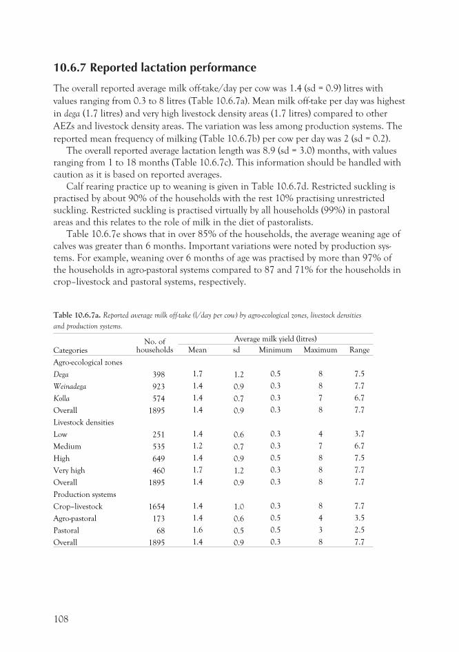
10.6.7 Reported lactation performance
The overall reported average milk off-take/day per cow was 1.4 (sd = 0.9) litres with
values ranging from 0.3 to 8 litres (Table 10.6.7a). Mean milk off-take per day was highest
in dega (1.7 litres) and very high livestock density areas (1.7 litres) compared to other
AEZs and livestock density areas. The variation was less among production systems. The
reported mean frequency of milking (Table 10.6.7b) per cow per day was 2 (sd = 0.2).
The overall reported average lactation length was 8.9 (sd = 3.0) months, with values
ranging from 1 to 18 months (Table 10.6.7c). This information should be handled with
caution as it is based on reported averages.
Calf rearing practice up to weaning is given in Table 10.6.7d. Restricted suckling is
practised by about 90% of the households with the rest 10% practising unrestricted
suckling. Restricted suckling is practised virtually by all households (99%) in pastoral
areas and this relates to the role of milk in the diet of pastoralists.
Table 10.6.7e shows that in over 85% of the households, the average weaning age of
calves was greater than 6 months. Important variations were noted by production sys-
tems. For example, weaning over 6 months of age was practised by more than 97% of
the households in agro-pastoral systems compared to 87 and 71% for the households in
crop–livestock and pastoral systems, respectively.
Table 10.6.7a. Reported average milk off-take (l/day per cow) by agro-ecological zones, livestock densities
and production systems.
CategoriesNo. of
households
Average milk yield (litres)
Mean sd Minimum Maximum Range
Agro-ecological zones
Dega 398 1.7 1.2 0.5 8 7.5
Weinadega 923 1.4 0.9 0.3 8 7.7
Kolla 574 1.4 0.7 0.3 7 6.7
Overall 1895 1.4 0.9 0.3 8 7.7
Livestock densities
Low 251 1.4 0.6 0.3 4 3.7
Medium 535 1.2 0.7 0.3 7 6.7
High 649 1.4 0.9 0.5 8 7.5
Very high 460 1.7 1.2 0.3 8 7.7
Overall 1895 1.4 0.9 0.3 8 7.7
Production systems
Crop–livestock 1654 1.4 1.0 0.3 8 7.7
Agro-pastoral 173 1.4 0.6 0.5 4 3.5
Pastoral 68 1.6 0.5 0.5 3 2.5
Overall 1895 1.4 0.9 0.3 8 7.7
108
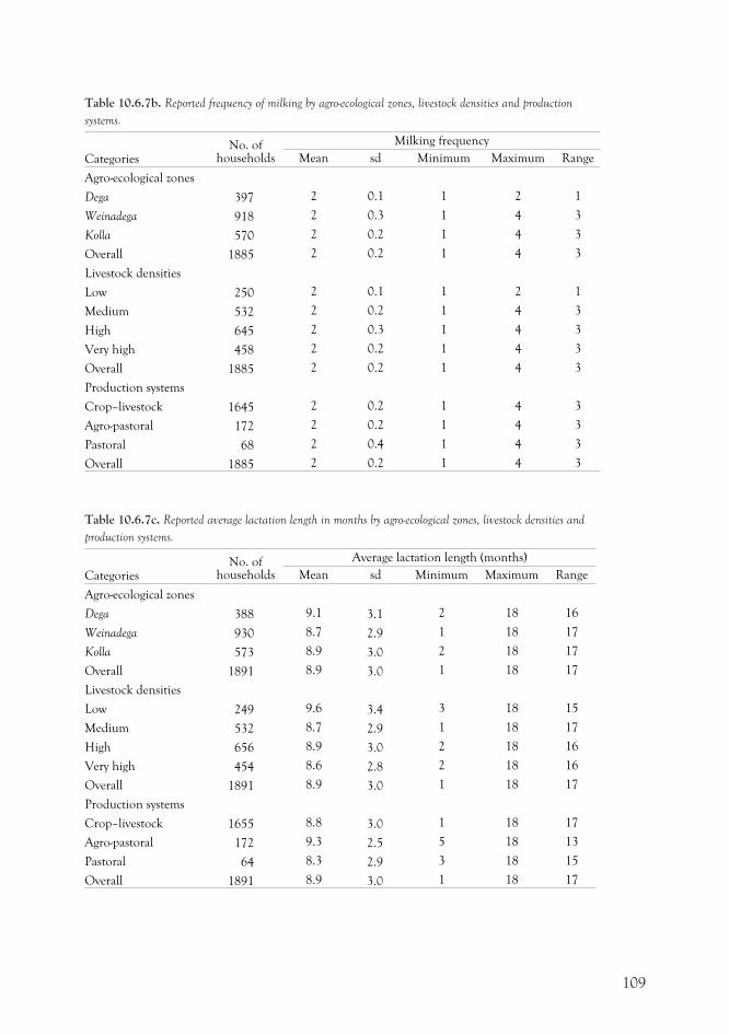
Table 10.6.7b. Reported frequency of milking by agro-ecological zones, livestock densities and production
systems.
CategoriesNo. of
households
Milking frequency
Mean sd Minimum Maximum Range
Agro-ecological zones
Dega 397 2 0.1 1 2 1
Weinadega 918 2 0.3 1 4 3
Kolla 570 2 0.2 1 4 3
Overall 1885 2 0.2 1 4 3
Livestock densities
Low 250 2 0.1 1 2 1
Medium 532 2 0.2 1 4 3
High 645 2 0.3 1 4 3
Very high 458 2 0.2 1 4 3
Overall 1885 2 0.2 1 4 3
Production systems
Crop–livestock 1645 2 0.2 1 4 3
Agro-pastoral 172 2 0.2 1 4 3
Pastoral 68 2 0.4 1 4 3
Overall 1885 2 0.2 1 4 3
Table 10.6.7c. Reported average lactation length in months by agro-ecological zones, livestock densities and
production systems.
CategoriesNo. of
households
Average lactation length (months)
Mean sd Minimum Maximum Range
Agro-ecological zones
Dega 388 9.1 3.1 2 18 16
Weinadega 930 8.7 2.9 1 18 17
Kolla 573 8.9 3.0 2 18 17
Overall 1891 8.9 3.0 1 18 17
Livestock densities
Low 249 9.6 3.4 3 18 15
Medium 532 8.7 2.9 1 18 17
High 656 8.9 3.0 2 18 16
Very high 454 8.6 2.8 2 18 16
Overall 1891 8.9 3.0 1 18 17
Production systems
Crop–livestock 1655 8.8 3.0 1 18 17
Agro-pastoral 172 9.3 2.5 5 18 13
Pastoral 64 8.3 2.9 3 18 15
Overall 1891 8.9 3.0 1 18 17
109
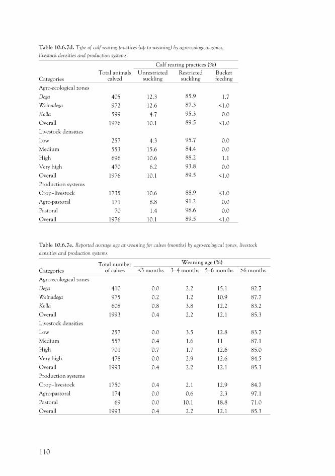
Table 10.6.7d. Type of calf rearing practices (up to weaning) by agro-ecological zones,
livestock densities and production systems.
CategoriesTotal animals
calved
Calf rearing practices (%)
Unrestrictedsuckling
Restrictedsuckling
Bucketfeeding
Agro-ecological zones
Dega 405 12.3 85.9 1.7
Weinadega 972 12.6 87.3 <1.0
Kolla 599 4.7 95.3 0.0
Overall 1976 10.1 89.5 <1.0
Livestock densities
Low 257 4.3 95.7 0.0
Medium 553 15.6 84.4 0.0
High 696 10.6 88.2 1.1
Very high 470 6.2 93.8 0.0
Overall 1976 10.1 89.5 <1.0
Production systems
Crop–livestock 1735 10.6 88.9 <1.0
Agro-pastoral 171 8.8 91.2 0.0
Pastoral 70 1.4 98.6 0.0
Overall 1976 10.1 89.5 <1.0
Table 10.6.7e. Reported average age at weaning for calves (months) by agro-ecological zones, livestock
densities and production systems.
CategoriesTotal number
of calves
Weaning age (%)
<3 months 3–4 months 5–6 months >6 months
Agro-ecological zones
Dega 410 0.0 2.2 15.1 82.7
Weinadega 975 0.2 1.2 10.9 87.7
Kolla 608 0.8 3.8 12.2 83.2
Overall 1993 0.4 2.2 12.1 85.3
Livestock densities
Low 257 0.0 3.5 12.8 83.7
Medium 557 0.4 1.6 11 87.1
High 701 0.7 1.7 12.6 85.0
Very high 478 0.0 2.9 12.6 84.5
Overall 1993 0.4 2.2 12.1 85.3
Production systems
Crop–livestock 1750 0.4 2.1 12.9 84.7
Agro-pastoral 174 0.0 0.6 2.3 97.1
Pastoral 69 0.0 10.1 18.8 71.0
Overall 1993 0.4 2.2 12.1 85.3
110
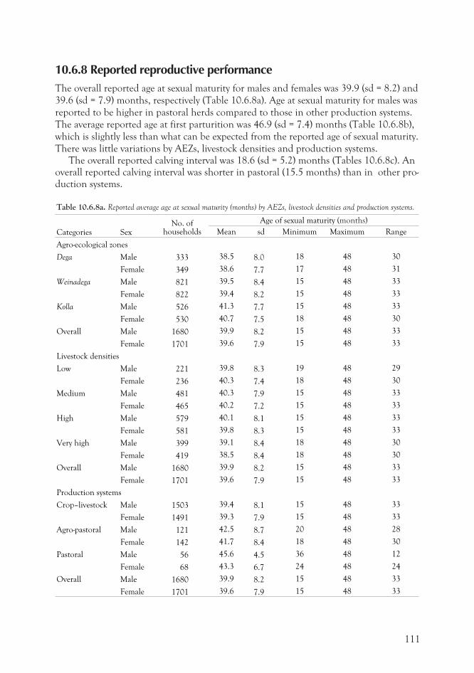
10.6.8 Reported reproductive performanceThe overall reported age at sexual maturity for males and females was 39.9 (sd = 8.2) and
39.6 (sd = 7.9) months, respectively (Table 10.6.8a). Age at sexual maturity for males was
reported to be higher in pastoral herds compared to those in other production systems.
The average reported age at first parturition was 46.9 (sd = 7.4) months (Table 10.6.8b),
which is slightly less than what can be expected from the reported age of sexual maturity.
There was little variations by AEZs, livestock densities and production systems.The overall reported calving interval was 18.6 (sd = 5.2) months (Tables 10.6.8c). An
overall reported calving interval was shorter in pastoral (15.5 months) than in other pro-duction systems.
Table 10.6.8a. Reported average age at sexual maturity (months) by AEZs, livestock densities and production systems.
Categories SexNo. of
households
Age of sexual maturity (months)
Mean sd Minimum Maximum Range
Agro-ecological zones
Dega Male 333 38.5 8.0 18 48 30
Female 349 38.6 7.7 17 48 31
Weinadega Male 821 39.5 8.4 15 48 33
Female 822 39.4 8.2 15 48 33
Kolla Male 526 41.3 7.7 15 48 33
Female 530 40.7 7.5 18 48 30
Overall Male 1680 39.9 8.2 15 48 33
Female 1701 39.6 7.9 15 48 33
Livestock densities
Low Male 221 39.8 8.3 19 48 29
Female 236 40.3 7.4 18 48 30
Medium Male 481 40.3 7.9 15 48 33
Female 465 40.2 7.2 15 48 33
High Male 579 40.1 8.1 15 48 33
Female 581 39.8 8.3 15 48 33
Very high Male 399 39.1 8.4 18 48 30
Female 419 38.5 8.4 18 48 30
Overall Male 1680 39.9 8.2 15 48 33
Female 1701 39.6 7.9 15 48 33
Production systems
Crop–livestock Male 1503 39.4 8.1 15 48 33
Female 1491 39.3 7.9 15 48 33
Agro-pastoral Male 121 42.5 8.7 20 48 28
Female 142 41.7 8.4 18 48 30
Pastoral Male 56 45.6 4.5 36 48 12
Female 68 43.3 6.7 24 48 24
Overall Male 1680 39.9 8.2 15 48 33
Female 1701 39.6 7.9 15 48 33
111
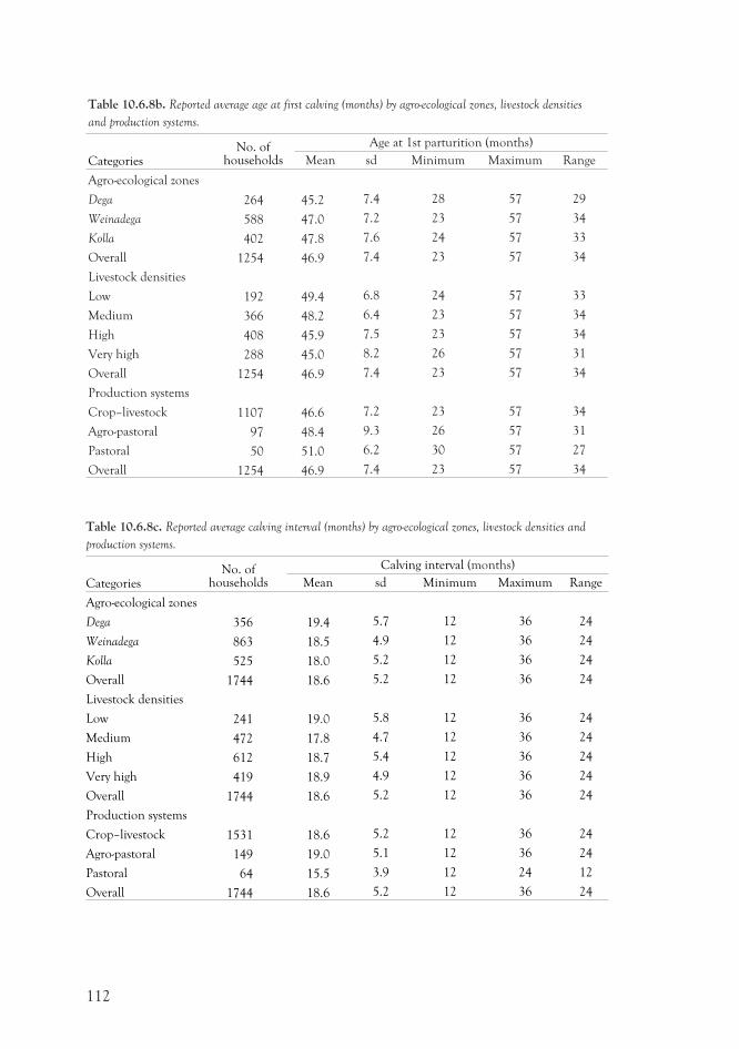
Table 10.6.8b. Reported average age at first calving (months) by agro-ecological zones, livestock densities
and production systems.
CategoriesNo. of
households
Age at 1st parturition (months)
Mean sd Minimum Maximum Range
Agro-ecological zones
Dega 264 45.2 7.4 28 57 29
Weinadega 588 47.0 7.2 23 57 34
Kolla 402 47.8 7.6 24 57 33
Overall 1254 46.9 7.4 23 57 34
Livestock densities
Low 192 49.4 6.8 24 57 33
Medium 366 48.2 6.4 23 57 34
High 408 45.9 7.5 23 57 34
Very high 288 45.0 8.2 26 57 31
Overall 1254 46.9 7.4 23 57 34
Production systems
Crop–livestock 1107 46.6 7.2 23 57 34
Agro-pastoral 97 48.4 9.3 26 57 31
Pastoral 50 51.0 6.2 30 57 27
Overall 1254 46.9 7.4 23 57 34
Table 10.6.8c. Reported average calving interval (months) by agro-ecological zones, livestock densities and
production systems.
CategoriesNo. of
households
Calving interval (months)
Mean sd Minimum Maximum Range
Agro-ecological zones
Dega 356 19.4 5.7 12 36 24
Weinadega 863 18.5 4.9 12 36 24
Kolla 525 18.0 5.2 12 36 24
Overall 1744 18.6 5.2 12 36 24
Livestock densities
Low 241 19.0 5.8 12 36 24
Medium 472 17.8 4.7 12 36 24
High 612 18.7 5.4 12 36 24
Very high 419 18.9 4.9 12 36 24
Overall 1744 18.6 5.2 12 36 24
Production systems
Crop–livestock 1531 18.6 5.2 12 36 24
Agro-pastoral 149 19.0 5.1 12 36 24
Pastoral 64 15.5 3.9 12 24 12
Overall 1744 18.6 5.2 12 36 24
112
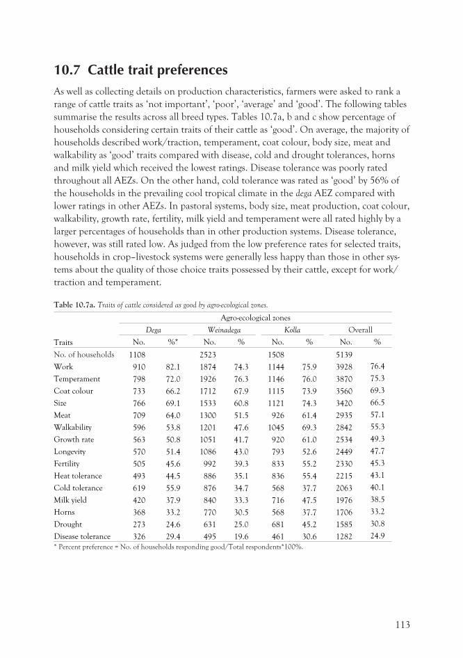
10.7 Cattle trait preferencesAs well as collecting details on production characteristics, farmers were asked to rank a
range of cattle traits as ‘not important’, ‘poor’, ‘average’ and ‘good’. The following tables
summarise the results across all breed types. Tables 10.7a, b and c show percentage of
households considering certain traits of their cattle as ‘good’. On average, the majority of
households described work/traction, temperament, coat colour, body size, meat and
walkability as ‘good’ traits compared with disease, cold and drought tolerances, horns
and milk yield which received the lowest ratings. Disease tolerance was poorly rated
throughout all AEZs. On the other hand, cold tolerance was rated as ‘good’ by 56% of
the households in the prevailing cool tropical climate in the dega AEZ compared with
lower ratings in other AEZs. In pastoral systems, body size, meat production, coat colour,
walkability, growth rate, fertility, milk yield and temperament were all rated highly by a
larger percentages of households than in other production systems. Disease tolerance,
however, was still rated low. As judged from the low preference rates for selected traits,
households in crop–livestock systems were generally less happy than those in other sys-
tems about the quality of those choice traits possessed by their cattle, except for work/
traction and temperament.
Table 10.7a. Traits of cattle considered as good by agro-ecological zones.
Traits
Agro-ecological zones
Dega Weinadega Kolla Overall
No. %* No. % No. % No. %
No. of households 1108 2523 1508 5139
Work 910 82.1 1874 74.3 1144 75.9 3928 76.4
Temperament 798 72.0 1926 76.3 1146 76.0 3870 75.3
Coat colour 733 66.2 1712 67.9 1115 73.9 3560 69.3
Size 766 69.1 1533 60.8 1121 74.3 3420 66.5
Meat 709 64.0 1300 51.5 926 61.4 2935 57.1
Walkability 596 53.8 1201 47.6 1045 69.3 2842 55.3
Growth rate 563 50.8 1051 41.7 920 61.0 2534 49.3
Longevity 570 51.4 1086 43.0 793 52.6 2449 47.7
Fertility 505 45.6 992 39.3 833 55.2 2330 45.3
Heat tolerance 493 44.5 886 35.1 836 55.4 2215 43.1
Cold tolerance 619 55.9 876 34.7 568 37.7 2063 40.1
Milk yield 420 37.9 840 33.3 716 47.5 1976 38.5
Horns 368 33.2 770 30.5 568 37.7 1706 33.2
Drought 273 24.6 631 25.0 681 45.2 1585 30.8
Disease tolerance 326 29.4 495 19.6 461 30.6 1282 24.9
* Percent preference = No. of households responding good/Total respondents*100%.
113
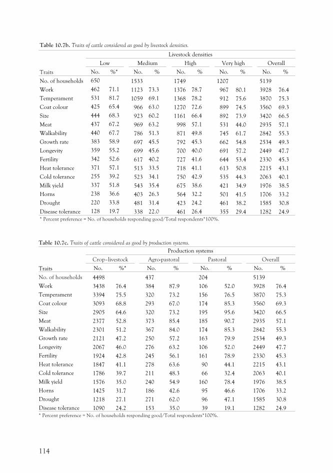
Table 10.7b. Traits of cattle considered as good by livestock densities.
Traits
Livestock densities
Low Medium High Very high Overall
No. %* No. % No. % No. % No. %
No. of households 650 1533 1749 1207 5139
Work 462 71.1 1123 73.3 1376 78.7 967 80.1 3928 76.4
Temperament 531 81.7 1059 69.1 1368 78.2 912 75.6 3870 75.3
Coat colour 425 65.4 966 63.0 1270 72.6 899 74.5 3560 69.3
Size 444 68.3 923 60.2 1161 66.4 892 73.9 3420 66.5
Meat 437 67.2 969 63.2 998 57.1 531 44.0 2935 57.1
Walkability 440 67.7 786 51.3 871 49.8 745 61.7 2842 55.3
Growth rate 383 58.9 697 45.5 792 45.3 662 54.8 2534 49.3
Longevity 359 55.2 699 45.6 700 40.0 691 57.2 2449 47.7
Fertility 342 52.6 617 40.2 727 41.6 644 53.4 2330 45.3
Heat tolerance 371 57.1 513 33.5 718 41.1 613 50.8 2215 43.1
Cold tolerance 255 39.2 523 34.1 750 42.9 535 44.3 2063 40.1
Milk yield 337 51.8 543 35.4 675 38.6 421 34.9 1976 38.5
Horns 238 36.6 403 26.3 564 32.2 501 41.5 1706 33.2
Drought 220 33.8 481 31.4 423 24.2 461 38.2 1585 30.8
Disease tolerance 128 19.7 338 22.0 461 26.4 355 29.4 1282 24.9
* Percent preference = No. of households responding good/Total respondents*100%.
Table 10.7c. Traits of cattle considered as good by production systems.
Traits
Production systems
Crop–livestock Agro-pastoral Pastoral Overall
No. %* No. % No. % No. %
No. of households 4498 437 204 5139
Work 3438 76.4 384 87.9 106 52.0 3928 76.4
Temperament 3394 75.5 320 73.2 156 76.5 3870 75.3
Coat colour 3093 68.8 293 67.0 174 85.3 3560 69.3
Size 2905 64.6 320 73.2 195 95.6 3420 66.5
Meat 2377 52.8 373 85.4 185 90.7 2935 57.1
Walkability 2301 51.2 367 84.0 174 85.3 2842 55.3
Growth rate 2121 47.2 250 57.2 163 79.9 2534 49.3
Longevity 2067 46.0 276 63.2 106 52.0 2449 47.7
Fertility 1924 42.8 245 56.1 161 78.9 2330 45.3
Heat tolerance 1847 41.1 278 63.6 90 44.1 2215 43.1
Cold tolerance 1786 39.7 211 48.3 66 32.4 2063 40.1
Milk yield 1576 35.0 240 54.9 160 78.4 1976 38.5
Horns 1425 31.7 186 42.6 95 46.6 1706 33.2
Drought 1218 27.1 271 62.0 96 47.1 1585 30.8
Disease tolerance 1090 24.2 153 35.0 39 19.1 1282 24.9
* Percent preference = No. of households responding good/Total respondents*100%.
114
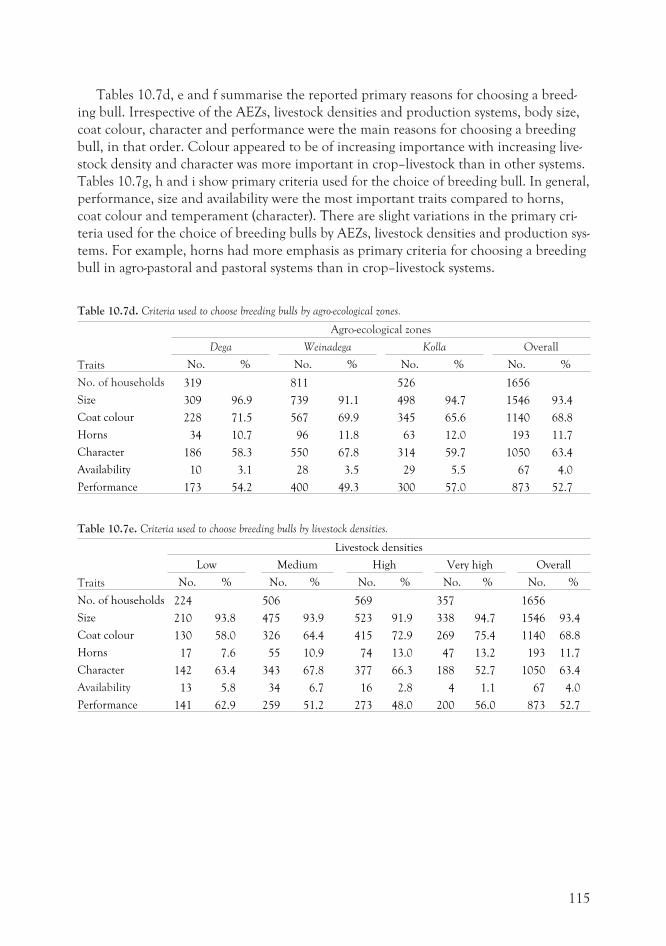
Tables 10.7d, e and f summarise the reported primary reasons for choosing a breed-
ing bull. Irrespective of the AEZs, livestock densities and production systems, body size,
coat colour, character and performance were the main reasons for choosing a breeding
bull, in that order. Colour appeared to be of increasing importance with increasing live-
stock density and character was more important in crop–livestock than in other systems.
Tables 10.7g, h and i show primary criteria used for the choice of breeding bull. In general,
performance, size and availability were the most important traits compared to horns,
coat colour and temperament (character). There are slight variations in the primary cri-
teria used for the choice of breeding bulls by AEZs, livestock densities and production sys-
tems. For example, horns had more emphasis as primary criteria for choosing a breeding
bull in agro-pastoral and pastoral systems than in crop–livestock systems.
Table 10.7d. Criteria used to choose breeding bulls by agro-ecological zones.
Traits
Agro-ecological zones
Dega Weinadega Kolla Overall
No. % No. % No. % No. %
No. of households 319 811 526 1656
Size 309 96.9 739 91.1 498 94.7 1546 93.4
Coat colour 228 71.5 567 69.9 345 65.6 1140 68.8
Horns 34 10.7 96 11.8 63 12.0 193 11.7
Character 186 58.3 550 67.8 314 59.7 1050 63.4
Availability 10 3.1 28 3.5 29 5.5 67 4.0
Performance 173 54.2 400 49.3 300 57.0 873 52.7
Table 10.7e. Criteria used to choose breeding bulls by livestock densities.
Traits
Livestock densities
Low Medium High Very high Overall
No. % No. % No. % No. % No. %
No. of households 224 506 569 357 1656
Size 210 93.8 475 93.9 523 91.9 338 94.7 1546 93.4
Coat colour 130 58.0 326 64.4 415 72.9 269 75.4 1140 68.8
Horns 17 7.6 55 10.9 74 13.0 47 13.2 193 11.7
Character 142 63.4 343 67.8 377 66.3 188 52.7 1050 63.4
Availability 13 5.8 34 6.7 16 2.8 4 1.1 67 4.0
Performance 141 62.9 259 51.2 273 48.0 200 56.0 873 52.7
115
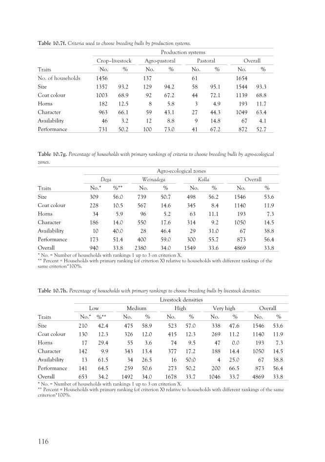
Table 10.7f. Criteria used to choose breeding bulls by production systems.
Traits
Production systems
Crop–livestock Agro-pastoral Pastoral Overall
No. % No. % No. % No. %
No. of households 1456 137 61 1654
Size 1357 93.2 129 94.2 58 95.1 1544 93.3
Coat colour 1003 68.9 92 67.2 44 72.1 1139 68.8
Horns 182 12.5 8 5.8 3 4.9 193 11.7
Character 963 66.1 59 43.1 27 44.3 1049 63.4
Availability 46 3.2 12 8.8 9 14.8 67 4.1
Performance 731 50.2 100 73.0 41 67.2 872 52.7
Table 10.7g. Percentage of households with primary rankings of criteria to choose breeding bulls by agro-ecological
zones.
Traits
Agro-ecological zones
Dega Weinadega Kolla Overall
No.* %** No. % No. % No. %
Size 309 56.0 739 50.7 498 56.2 1546 53.6
Coat colour 228 10.5 567 14.6 345 8.4 1140 11.9
Horns 34 5.9 96 5.2 63 11.1 193 7.3
Character 186 14.0 550 17.6 314 9.2 1050 14.5
Availability 10 40.0 28 46.4 29 31.0 67 38.8
Performance 173 51.4 400 59.0 300 55.7 873 56.4
Overall 940 33.8 2380 34.0 1549 33.6 4869 33.8
* No. = Number of households with rankings 1 up to 3 on criterion X.** Percent = Households with primary ranking (of criterion X) relative to households with different rankings of thesame criterion*100%.
Table 10.7h. Percentage of households with primary rankings to choose breeding bulls by livestock densities.
Traits
Livestock densities
Low Medium High Very high Overall
No.* %** No. % No. % No. % No. %
Size 210 42.4 475 58.9 523 57.0 338 47.6 1546 53.6
Coat colour 130 12.3 326 12.0 415 12.3 269 11.2 1140 11.9
Horns 17 29.4 55 3.6 74 9.5 47 0.0 193 7.3
Character 142 9.9 343 13.4 377 17.2 188 14.4 1050 14.5
Availability 13 61.5 34 26.5 16 50.0 4 25.0 67 38.8
Performance 141 64.5 259 50.6 273 50.2 200 66.5 873 56.4
Overall 653 34.2 1492 34.0 1678 33.7 1046 33.7 4869 33.8
* No. = Number of households with rankings 1 up to 3 on criterion X.** Percent = Households with primary ranking (of criterion X) relative to households with different rankings of the samecriterion*100%.
116
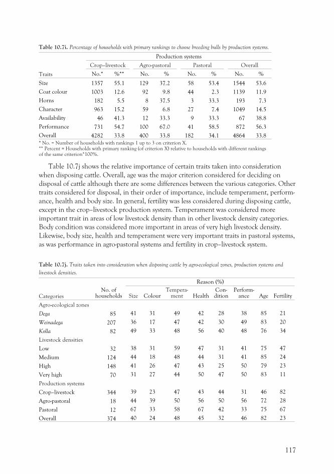
Table 10.7i. Percentage of households with primary rankings to choose breeding bulls by production systems.
Traits
Production systems
Crop–livestock Agro-pastoral Pastoral Overall
No.* %** No. % No. % No. %
Size 1357 55.1 129 37.2 58 53.4 1544 53.6
Coat colour 1003 12.6 92 9.8 44 2.3 1139 11.9
Horns 182 5.5 8 37.5 3 33.3 193 7.3
Character 963 15.2 59 6.8 27 7.4 1049 14.5
Availability 46 41.3 12 33.3 9 33.3 67 38.8
Performance 731 54.7 100 67.0 41 58.5 872 56.3
Overall 4282 33.8 400 33.8 182 34.1 4864 33.8
* No. = Number of households with rankings 1 up to 3 on criterion X.** Percent = Households with primary ranking (of criterion X) relative to households with different rankingsof the same criterion*100%.
Table 10.7j shows the relative importance of certain traits taken into consideration
when disposing cattle. Overall, age was the major criterion considered for deciding on
disposal of cattle although there are some differences between the various categories. Other
traits considered for disposal, in their order of importance, include temperament, perform-
ance, health and body size. In general, fertility was less considered during disposing cattle,
except in the crop–livestock production system. Temperament was considered more
important trait in areas of low livestock density than in other livestock density categories.
Body condition was considered more important in areas of very high livestock density.
Likewise, body size, health and temperament were very important traits in pastoral systems,
as was performance in agro-pastoral systems and fertility in crop–livestock system.
Table 10.7j. Traits taken into consideration when disposing cattle by agro-ecological zones, production systems and
livestock densities.
CategoriesNo. of
households
Reason (%)
Size ColourTempera-
ment HealthCon-dition
Perform-ance Age Fertility
Agro-ecological zones
Dega 85 41 31 49 42 28 38 85 21
Weinadega 207 36 17 47 42 30 49 83 20
Kolla 82 49 33 48 56 40 48 76 34
Livestock densities
Low 32 38 31 59 47 31 41 75 47
Medium 124 44 18 48 44 31 41 85 24
High 148 41 26 47 43 25 50 79 23
Very high 70 31 27 44 50 47 50 83 11
Production systems
Crop–livestock 344 39 23 47 43 44 31 46 82
Agro-pastoral 18 44 39 50 56 50 56 72 28
Pastoral 12 67 33 58 67 42 33 75 67
Overall 374 40 24 48 45 32 46 82 23
117
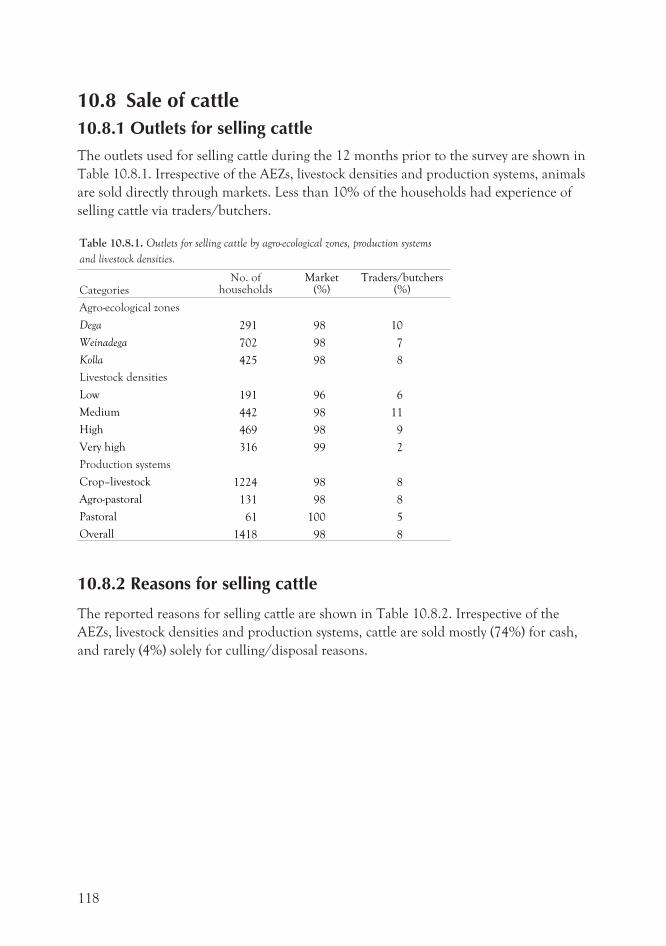
10.8 Sale of cattle10.8.1 Outlets for selling cattle
The outlets used for selling cattle during the 12 months prior to the survey are shown in
Table 10.8.1. Irrespective of the AEZs, livestock densities and production systems, animals
are sold directly through markets. Less than 10% of the households had experience of
selling cattle via traders/butchers.
Table 10.8.1. Outlets for selling cattle by agro-ecological zones, production systems
and livestock densities.
CategoriesNo. of
householdsMarket
(%)Traders/butchers
(%)
Agro-ecological zones
Dega 291 98 10
Weinadega 702 98 7
Kolla 425 98 8
Livestock densities
Low 191 96 6
Medium 442 98 11
High 469 98 9
Very high 316 99 2
Production systems
Crop–livestock 1224 98 8
Agro-pastoral 131 98 8
Pastoral 61 100 5
Overall 1418 98 8
10.8.2 Reasons for selling cattle
The reported reasons for selling cattle are shown in Table 10.8.2. Irrespective of the
AEZs, livestock densities and production systems, cattle are sold mostly (74%) for cash,
and rarely (4%) solely for culling/disposal reasons.
118
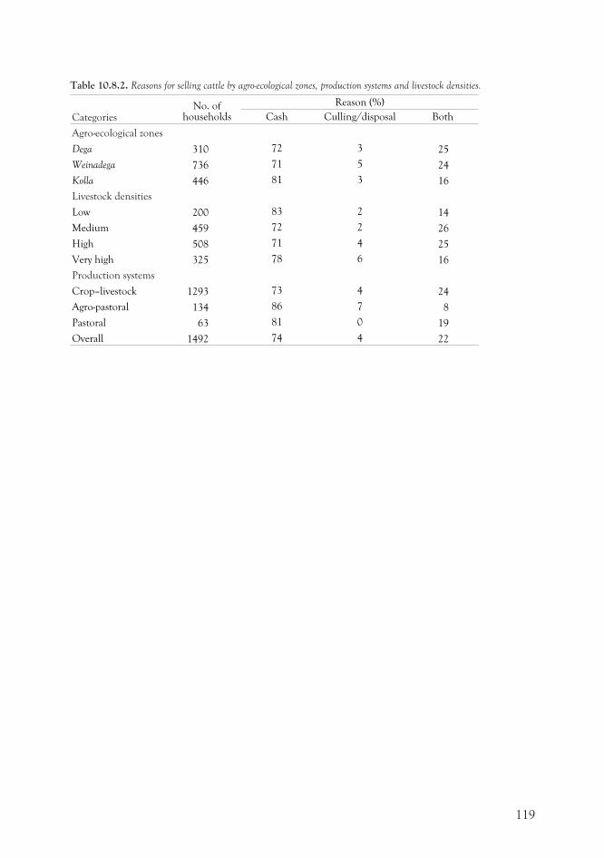
Table 10.8.2. Reasons for selling cattle by agro-ecological zones, production systems and livestock densities.
CategoriesNo. of
households
Reason (%)
Cash Culling/disposal Both
Agro-ecological zones
Dega 310 72 3 25
Weinadega 736 71 5 24
Kolla 446 81 3 16
Livestock densities
Low 200 83 2 14
Medium 459 72 2 26
High 508 71 4 25
Very high 325 78 6 16
Production systems
Crop–livestock 1293 73 4 24
Agro-pastoral 134 86 7 8
Pastoral 63 81 0 19
Overall 1492 74 4 22
119
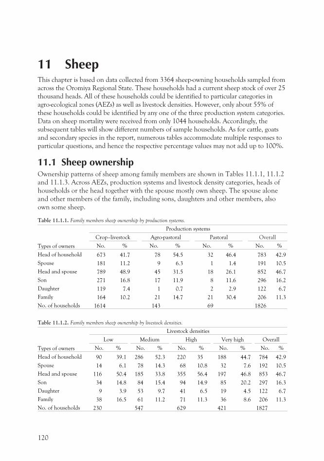
11 SheepThis chapter is based on data collected from 3364 sheep-owning households sampled from
across the Oromiya Regional State. These households had a current sheep stock of over 25
thousand heads. All of these households could be identified to particular categories in
agro-ecological zones (AEZs) as well as livestock densities. However, only about 55% of
these households could be identified by any one of the three production system categories.
Data on sheep mortality were received from only 1044 households. Accordingly, the
subsequent tables will show different numbers of sample households. As for cattle, goats
and secondary species in the report, numerous tables accommodate multiple responses to
particular questions, and hence the respective percentage values may not add up to 100%.
11.1 Sheep ownershipOwnership patterns of sheep among family members are shown in Tables 11.1.1, 11.1.2
and 11.1.3. Across AEZs, production systems and livestock density categories, heads of
households or the head together with the spouse mostly own sheep. The spouse alone
and other members of the family, including sons, daughters and other members, also
own some sheep.
Table 11.1.1. Family members sheep ownership by production systems.
Types of owners
Production systems
Crop–livestock Agro-pastoral Pastoral Overall
No. % No. % No. % No. %
Head of household 673 41.7 78 54.5 32 46.4 783 42.9
Spouse 181 11.2 9 6.3 1 1.4 191 10.5
Head and spouse 789 48.9 45 31.5 18 26.1 852 46.7
Son 271 16.8 17 11.9 8 11.6 296 16.2
Daughter 119 7.4 1 0.7 2 2.9 122 6.7
Family 164 10.2 21 14.7 21 30.4 206 11.3
No. of households 1614 143 69 1826
Table 11.1.2. Family members sheep ownership by livestock densities.
Types of owners
Livestock densities
Low Medium High Very high Overall
No. % No. % No. % No. % No. %
Head of household 90 39.1 286 52.3 220 35 188 44.7 784 42.9
Spouse 14 6.1 78 14.3 68 10.8 32 7.6 192 10.5
Head and spouse 116 50.4 185 33.8 355 56.4 197 46.8 853 46.7
Son 34 14.8 84 15.4 94 14.9 85 20.2 297 16.3
Daughter 9 3.9 53 9.7 41 6.5 19 4.5 122 6.7
Family 38 16.5 61 11.2 71 11.3 36 8.6 206 11.3
No. of households 230 547 629 421 1827
120
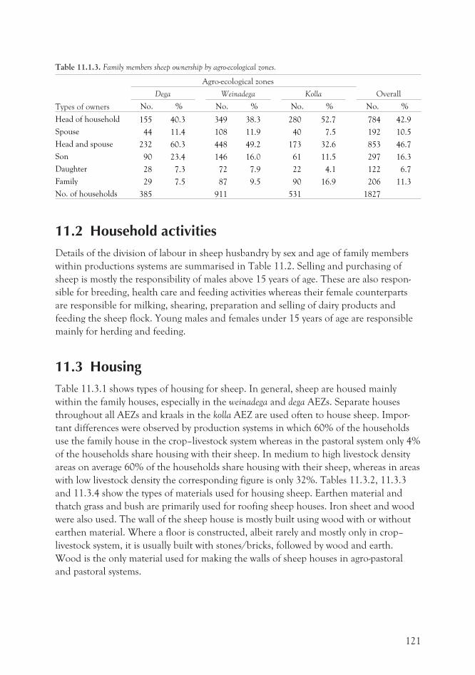
Table 11.1.3. Family members sheep ownership by agro-ecological zones.
Types of owners
Agro-ecological zones
OverallDega Weinadega Kolla
No. % No. % No. % No. %
Head of household 155 40.3 349 38.3 280 52.7 784 42.9
Spouse 44 11.4 108 11.9 40 7.5 192 10.5
Head and spouse 232 60.3 448 49.2 173 32.6 853 46.7
Son 90 23.4 146 16.0 61 11.5 297 16.3
Daughter 28 7.3 72 7.9 22 4.1 122 6.7
Family 29 7.5 87 9.5 90 16.9 206 11.3
No. of households 385 911 531 1827
11.2 Household activitiesDetails of the division of labour in sheep husbandry by sex and age of family members
within productions systems are summarised in Table 11.2. Selling and purchasing of
sheep is mostly the responsibility of males above 15 years of age. These are also respon-
sible for breeding, health care and feeding activities whereas their female counterparts
are responsible for milking, shearing, preparation and selling of dairy products and
feeding the sheep flock. Young males and females under 15 years of age are responsible
mainly for herding and feeding.
11.3 HousingTable 11.3.1 shows types of housing for sheep. In general, sheep are housed mainly
within the family houses, especially in the weinadega and dega AEZs. Separate houses
throughout all AEZs and kraals in the kolla AEZ are used often to house sheep. Impor-
tant differences were observed by production systems in which 60% of the households
use the family house in the crop–livestock system whereas in the pastoral system only 4%
of the households share housing with their sheep. In medium to high livestock density
areas on average 60% of the households share housing with their sheep, whereas in areas
with low livestock density the corresponding figure is only 32%. Tables 11.3.2, 11.3.3
and 11.3.4 show the types of materials used for housing sheep. Earthen material and
thatch grass and bush are primarily used for roofing sheep houses. Iron sheet and wood
were also used. The wall of the sheep house is mostly built using wood with or without
earthen material. Where a floor is constructed, albeit rarely and mostly only in crop–
livestock system, it is usually built with stones/bricks, followed by wood and earth.
Wood is the only material used for making the walls of sheep houses in agro-pastoral
and pastoral systems.
121
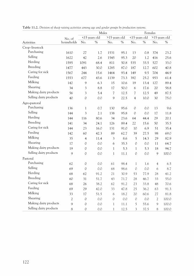
Table 11.2. Division of sheep raising activities among age and gender groups by production systems.
ActivitiesNo. of
households
Males Females
<15 years old >15 years old <15 years old >15 years old
No. % No. % No. % No. %
Crop–livestock
Purchasing 1610 27 1.7 1531 95.1 13 0.8 374 23.2
Selling 1622 42 2.6 1545 95.3 20 1.2 416 25.6
Herding 1595 1091 68.4 811 50.8 535 33.5 527 33.0
Breeding 1477 443 30.0 1285 87.0 187 12.7 602 40.8
Caring for sick 1567 244 15.6 1464 93.4 149 9.5 704 44.9
Feeding 1553 677 43.6 1139 73.3 392 25.2 953 61.4
Milking 142 9 6.3 15 10.6 19 13.4 127 89.4
Shearing 34 3 8.8 17 50.0 6 17.6 20 58.8
Making dairy products 56 3 5.4 7 12.5 7 12.5 49 87.5
Selling dairy products 40 0 0.0 9 22.5 4 10.0 30 75.0
Agro-pastoral
Purchasing 136 1 0.7 130 95.6 0 0.0 13 9.6
Selling 144 3 2.1 138 95.8 0 0.0 17 11.8
Herding 144 116 80.6 34 23.6 64 44.4 29 20.1
Breeding 141 34 24.1 126 89.4 22 15.6 50 35.5
Caring for sick 144 23 16.0 131 91.0 10 6.9 51 35.4
Feeding 142 60 42.3 89 62.7 39 27.5 98 69.0
Milking 35 4 11.4 3 8.6 5 14.3 29 82.9
Shearing 17 0 0.0 6 35.3 0 0.0 11 64.7
Making dairy products 19 0 0.0 1 5.3 1 5.3 18 94.7
Selling dairy products 9 0 0.0 1 11.1 0 0.0 9 100.0
Pastoral
Purchasing 62 0 0.0 61 98.4 1 1.6 4 6.5
Selling 69 0 0.0 68 98.6 0 0.0 6 8.7
Herding 68 62 91.2 21 30.9 53 77.9 28 41.2
Breeding 60 31 51.7 43 71.7 28 46.7 33 55.0
Caring for sick 68 26 38.2 62 91.2 23 33.8 48 70.6
Feeding 69 29 42.0 33 47.8 25 36.2 63 91.3
Milking 33 17 51.5 6 18.2 20 60.6 27 81.8
Shearing 2 0 0.0 0 0.0 0 0.0 2 100.0
Making dairy products 9 0 0.0 1 11.1 5 55.6 9 100.0
Selling dairy products 8 0 0.0 1 12.5 3 37.5 8 100.0
122
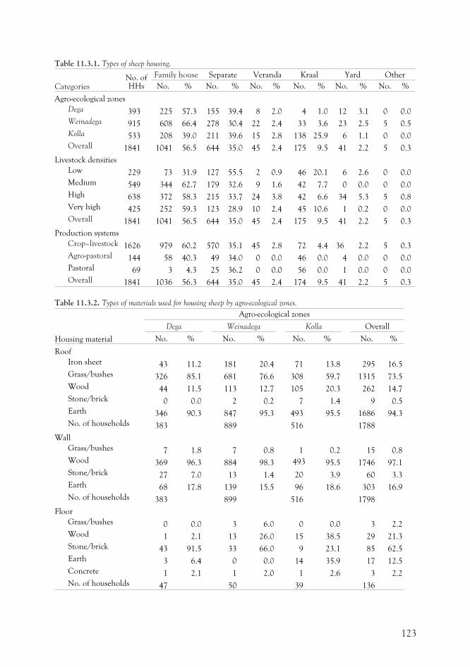
Table 11.3.1. Types of sheep housing.
CategoriesNo. ofHHs
Family house Separate Veranda Kraal Yard Other
No. % No. % No. % No. % No. % No. %
Agro-ecological zones
Dega 393 225 57.3 155 39.4 8 2.0 4 1.0 12 3.1 0 0.0
Weinadega 915 608 66.4 278 30.4 22 2.4 33 3.6 23 2.5 5 0.5
Kolla 533 208 39.0 211 39.6 15 2.8 138 25.9 6 1.1 0 0.0
Overall 1841 1041 56.5 644 35.0 45 2.4 175 9.5 41 2.2 5 0.3
Livestock densities
Low 229 73 31.9 127 55.5 2 0.9 46 20.1 6 2.6 0 0.0
Medium 549 344 62.7 179 32.6 9 1.6 42 7.7 0 0.0 0 0.0
High 638 372 58.3 215 33.7 24 3.8 42 6.6 34 5.3 5 0.8
Very high 425 252 59.3 123 28.9 10 2.4 45 10.6 1 0.2 0 0.0
Overall 1841 1041 56.5 644 35.0 45 2.4 175 9.5 41 2.2 5 0.3
Production systems
Crop–livestock 1626 979 60.2 570 35.1 45 2.8 72 4.4 36 2.2 5 0.3
Agro-pastoral 144 58 40.3 49 34.0 0 0.0 46 0.0 4 0.0 0 0.0
Pastoral 69 3 4.3 25 36.2 0 0.0 56 0.0 1 0.0 0 0.0
Overall 1841 1036 56.3 644 35.0 45 2.4 174 9.5 41 2.2 5 0.3
Table 11.3.2. Types of materials used for housing sheep by agro-ecological zones.
Housing material
Agro-ecological zones
Dega Weinadega Kolla Overall
No. % No. % No. % No. %
Roof
Iron sheet 43 11.2 181 20.4 71 13.8 295 16.5
Grass/bushes 326 85.1 681 76.6 308 59.7 1315 73.5
Wood 44 11.5 113 12.7 105 20.3 262 14.7
Stone/brick 0 0.0 2 0.2 7 1.4 9 0.5
Earth 346 90.3 847 95.3 493 95.5 1686 94.3
No. of households 383 889 516 1788
Wall
Grass/bushes 7 1.8 7 0.8 1 0.2 15 0.8
Wood 369 96.3 884 98.3 493 95.5 1746 97.1
Stone/brick 27 7.0 13 1.4 20 3.9 60 3.3
Earth 68 17.8 139 15.5 96 18.6 303 16.9
No. of households 383 899 516 1798
Floor
Grass/bushes 0 0.0 3 6.0 0 0.0 3 2.2
Wood 1 2.1 13 26.0 15 38.5 29 21.3
Stone/brick 43 91.5 33 66.0 9 23.1 85 62.5
Earth 3 6.4 0 0.0 14 35.9 17 12.5
Concrete 1 2.1 1 2.0 1 2.6 3 2.2
No. of households 47 50 39 136
123
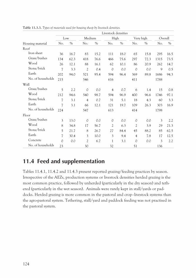
Table 11.3.3. Types of materials used for housing sheep by livestock densities.
Housing material
Livestock densities
Low Medium High Very high Overall
No. % No. % No. % No. % No. %
Roof
Iron sheet 36 16.7 83 15.2 111 18.0 65 15.8 295 16.5
Grass/bushes 134 62.3 418 76.6 466 75.6 297 72.3 1315 73.5
Wood 26 12.1 88 16.1 62 10.1 86 20.9 262 14.7
Stone/brick 7 3.3 2 0.4 0 0.0 0 0.0 9 0.5
Earth 202 94.0 521 95.4 594 96.4 369 89.8 1686 94.3
No. of households 215 546 616 411 1788
Wall
Grass/bushes 5 2.2 0 0.0 4 0.7 6 1.4 15 0.8
Wood 212 94.6 540 98.7 594 96.9 400 96.6 1746 97.1
Stone/brick 7 3.1 4 0.7 31 5.1 18 4.3 60 3.3
Earth 7 3.1 66 12.1 121 19.7 109 26.3 303 16.9
No. of households 224 547 613 414 1798
Floor
Grass/bushes 3 13.0 0 0.0 0 0.0 0 0.0 3 2.2
Wood 8 34.8 17 56.7 2 6.3 2 3.9 29 21.3
Stone/brick 5 21.7 8 26.7 27 84.4 45 88.2 85 62.5
Earth 7 30.4 3 10.0 3 9.4 4 7.8 17 12.5
Concrete 0 0.0 2 6.7 1 3.1 0 0.0 3 2.2
No. of households 23 30 32 51 136
11.4 Feed and supplementation
Tables 11.4.1, 11.4.2 and 11.4.3 present reported grazing/feeding practices by season.
Irrespective of the AEZs, production systems or livestock densities herded grazing is the
most common practice, followed by unherded (particularly in the dry season) and teth-
ered (particularly in the wet season). Animals were rarely kept in stall/yards or pad-
docks. Herded grazing is more common in the pastoral and crop–livestock systems than
the agro-pastoral system. Tethering, stall/yard and paddock feeding was not practised in
the pastoral system.
124
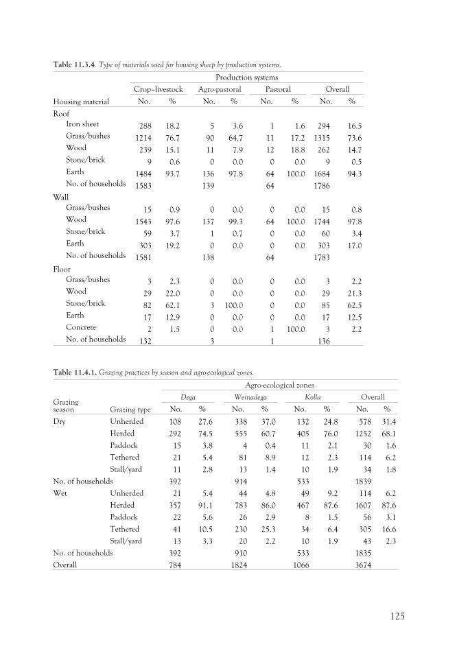
Table 11.3.4. Type of materials used for housing sheep by production systems.
Housing material
Production systems
Crop–livestock Agro-pastoral Pastoral Overall
No. % No. % No. % No. %
Roof
Iron sheet 288 18.2 5 3.6 1 1.6 294 16.5
Grass/bushes 1214 76.7 90 64.7 11 17.2 1315 73.6
Wood 239 15.1 11 7.9 12 18.8 262 14.7
Stone/brick 9 0.6 0 0.0 0 0.0 9 0.5
Earth 1484 93.7 136 97.8 64 100.0 1684 94.3
No. of households 1583 139 64 1786
Wall
Grass/bushes 15 0.9 0 0.0 0 0.0 15 0.8
Wood 1543 97.6 137 99.3 64 100.0 1744 97.8
Stone/brick 59 3.7 1 0.7 0 0.0 60 3.4
Earth 303 19.2 0 0.0 0 0.0 303 17.0
No. of households 1581 138 64 1783
Floor
Grass/bushes 3 2.3 0 0.0 0 0.0 3 2.2
Wood 29 22.0 0 0.0 0 0.0 29 21.3
Stone/brick 82 62.1 3 100.0 0 0.0 85 62.5
Earth 17 12.9 0 0.0 0 0.0 17 12.5
Concrete 2 1.5 0 0.0 1 100.0 3 2.2
No. of households 132 3 1 136
Table 11.4.1. Grazing practices by season and agro-ecological zones.
Grazingseason Grazing type
Agro-ecological zones
Dega Weinadega Kolla Overall
No. % No. % No. % No. %
Dry Unherded 108 27.6 338 37.0 132 24.8 578 31.4
Herded 292 74.5 555 60.7 405 76.0 1252 68.1
Paddock 15 3.8 4 0.4 11 2.1 30 1.6
Tethered 21 5.4 81 8.9 12 2.3 114 6.2
Stall/yard 11 2.8 13 1.4 10 1.9 34 1.8
No. of households 392 914 533 1839
Wet Unherded 21 5.4 44 4.8 49 9.2 114 6.2
Herded 357 91.1 783 86.0 467 87.6 1607 87.6
Paddock 22 5.6 26 2.9 8 1.5 56 3.1
Tethered 41 10.5 230 25.3 34 6.4 305 16.6
Stall/yard 13 3.3 20 2.2 10 1.9 43 2.3
No. of households 392 910 533 1835
Overall 784 1824 1066 3674
125
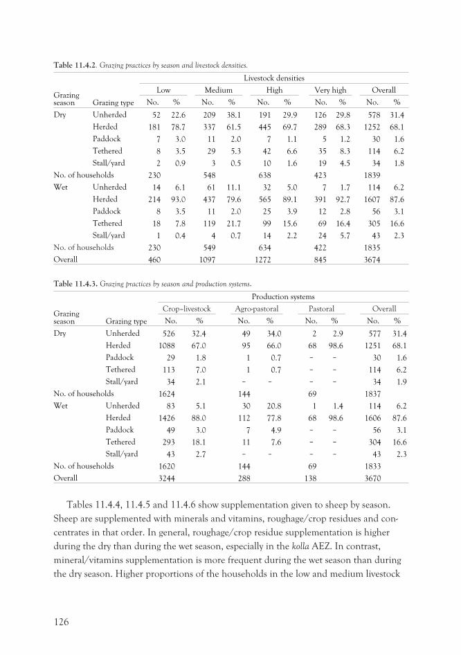
Table 11.4.2. Grazing practices by season and livestock densities.
Grazingseason Grazing type
Livestock densities
Low Medium High Very high Overall
No. % No. % No. % No. % No. %
Dry Unherded 52 22.6 209 38.1 191 29.9 126 29.8 578 31.4
Herded 181 78.7 337 61.5 445 69.7 289 68.3 1252 68.1
Paddock 7 3.0 11 2.0 7 1.1 5 1.2 30 1.6
Tethered 8 3.5 29 5.3 42 6.6 35 8.3 114 6.2
Stall/yard 2 0.9 3 0.5 10 1.6 19 4.5 34 1.8
No. of households 230 548 638 423 1839
Wet Unherded 14 6.1 61 11.1 32 5.0 7 1.7 114 6.2
Herded 214 93.0 437 79.6 565 89.1 391 92.7 1607 87.6
Paddock 8 3.5 11 2.0 25 3.9 12 2.8 56 3.1
Tethered 18 7.8 119 21.7 99 15.6 69 16.4 305 16.6
Stall/yard 1 0.4 4 0.7 14 2.2 24 5.7 43 2.3
No. of households 230 549 634 422 1835
Overall 460 1097 1272 845 3674
Table 11.4.3. Grazing practices by season and production systems.
Grazingseason Grazing type
Production systems
Crop–livestock Agro-pastoral Pastoral Overall
No. % No. % No. % No. %
Dry Unherded 526 32.4 49 34.0 2 2.9 577 31.4
Herded 1088 67.0 95 66.0 68 98.6 1251 68.1
Paddock 29 1.8 1 0.7 – – 30 1.6
Tethered 113 7.0 1 0.7 – – 114 6.2
Stall/yard 34 2.1 – – – – 34 1.9
No. of households 1624 144 69 1837
Wet Unherded 83 5.1 30 20.8 1 1.4 114 6.2
Herded 1426 88.0 112 77.8 68 98.6 1606 87.6
Paddock 49 3.0 7 4.9 – – 56 3.1
Tethered 293 18.1 11 7.6 – – 304 16.6
Stall/yard 43 2.7 – – – – 43 2.3
No. of households 1620 144 69 1833
Overall 3244 288 138 3670
Tables 11.4.4, 11.4.5 and 11.4.6 show supplementation given to sheep by season.
Sheep are supplemented with minerals and vitamins, roughage/crop residues and con-
centrates in that order. In general, roughage/crop residue supplementation is higher
during the dry than during the wet season, especially in the kolla AEZ. In contrast,
mineral/vitamins supplementation is more frequent during the wet season than during
the dry season. Higher proportions of the households in the low and medium livestock
126
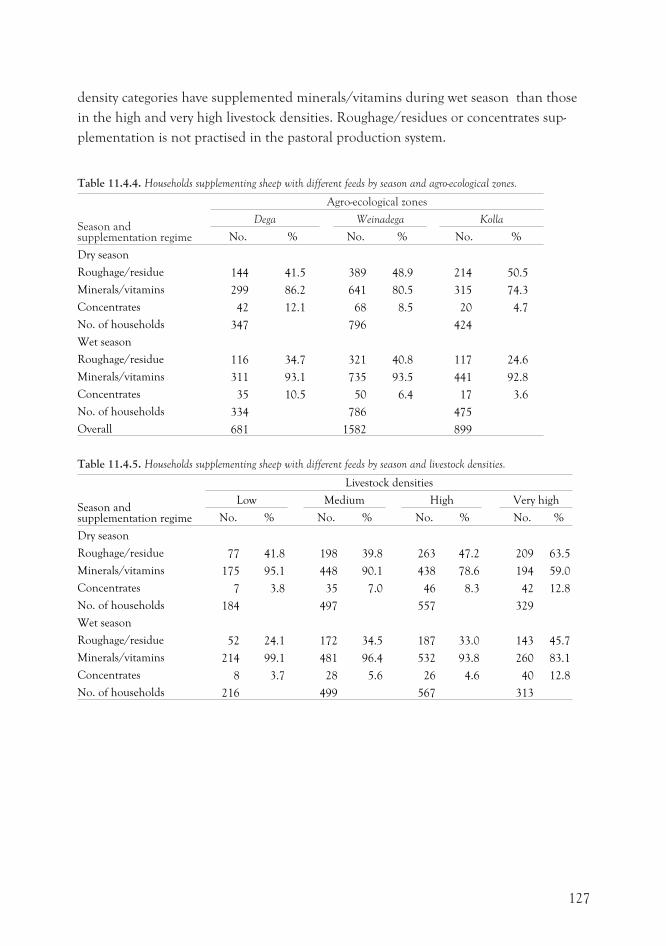
density categories have supplemented minerals/vitamins during wet season than those
in the high and very high livestock densities. Roughage/residues or concentrates sup-
plementation is not practised in the pastoral production system.
Table 11.4.4. Households supplementing sheep with different feeds by season and agro-ecological zones.
Season andsupplementation regime
Agro-ecological zones
Dega Weinadega Kolla
No. % No. % No. %
Dry season
Roughage/residue 144 41.5 389 48.9 214 50.5
Minerals/vitamins 299 86.2 641 80.5 315 74.3
Concentrates 42 12.1 68 8.5 20 4.7
No. of households 347 796 424
Wet season
Roughage/residue 116 34.7 321 40.8 117 24.6
Minerals/vitamins 311 93.1 735 93.5 441 92.8
Concentrates 35 10.5 50 6.4 17 3.6
No. of households 334 786 475
Overall 681 1582 899
Table 11.4.5. Households supplementing sheep with different feeds by season and livestock densities.
Season andsupplementation regime
Livestock densities
Low Medium High Very high
No. % No. % No. % No. %
Dry season
Roughage/residue 77 41.8 198 39.8 263 47.2 209 63.5
Minerals/vitamins 175 95.1 448 90.1 438 78.6 194 59.0
Concentrates 7 3.8 35 7.0 46 8.3 42 12.8
No. of households 184 497 557 329
Wet season
Roughage/residue 52 24.1 172 34.5 187 33.0 143 45.7
Minerals/vitamins 214 99.1 481 96.4 532 93.8 260 83.1
Concentrates 8 3.7 28 5.6 26 4.6 40 12.8
No. of households 216 499 567 313
127
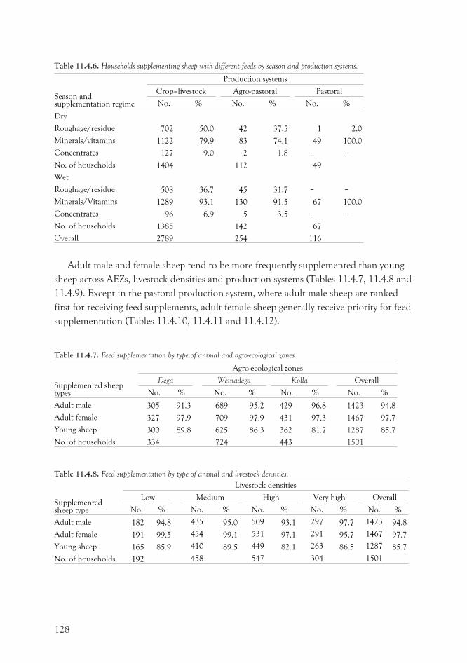
Table 11.4.6. Households supplementing sheep with different feeds by season and production systems.
Season andsupplementation regime
Production systems
Crop–livestock Agro-pastoral Pastoral
No. % No. % No. %
Dry
Roughage/residue 702 50.0 42 37.5 1 2.0
Minerals/vitamins 1122 79.9 83 74.1 49 100.0
Concentrates 127 9.0 2 1.8 – –
No. of households 1404 112 49
Wet
Roughage/residue 508 36.7 45 31.7 – –
Minerals/Vitamins 1289 93.1 130 91.5 67 100.0
Concentrates 96 6.9 5 3.5 – –
No. of households 1385 142 67
Overall 2789 254 116
Adult male and female sheep tend to be more frequently supplemented than young
sheep across AEZs, livestock densities and production systems (Tables 11.4.7, 11.4.8 and
11.4.9). Except in the pastoral production system, where adult male sheep are ranked
first for receiving feed supplements, adult female sheep generally receive priority for feed
supplementation (Tables 11.4.10, 11.4.11 and 11.4.12).
Table 11.4.7. Feed supplementation by type of animal and agro-ecological zones.
Supplemented sheeptypes
Agro-ecological zones
Dega Weinadega Kolla Overall
No. % No. % No. % No. %
Adult male 305 91.3 689 95.2 429 96.8 1423 94.8
Adult female 327 97.9 709 97.9 431 97.3 1467 97.7
Young sheep 300 89.8 625 86.3 362 81.7 1287 85.7
No. of households 334 724 443 1501
Table 11.4.8. Feed supplementation by type of animal and livestock densities.
Supplementedsheep type
Livestock densities
Low Medium High Very high Overall
No. % No. % No. % No. % No. %
Adult male 182 94.8 435 95.0 509 93.1 297 97.7 1423 94.8
Adult female 191 99.5 454 99.1 531 97.1 291 95.7 1467 97.7
Young sheep 165 85.9 410 89.5 449 82.1 263 86.5 1287 85.7
No. of households 192 458 547 304 1501
128
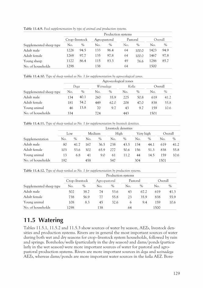
Table 11.4.9. Feed supplementation by type of animal and production systems.
Supplemented sheep type
Production systems
Crop–livestock Agro-pastoral Pastoral Overall
No. % No. % No. % No. %
Adult male 1226 94.5 133 96.4 64 100.0 1423 94.9
Adult female 1268 97.7 135 97.8 64 100.0 1467 97.8
Young sheep 1122 86.4 115 83.3 49 76.6 1286 85.7
No. of households 1298 138 64 1500
Table 11.4.10. Type of sheep ranked as No. 1 for supplementation by agro-ecological zones.
Supplemented sheep type
Agro-ecological zones
Dega Weinadega Kolla Overall
No. % No. % No. % No. %
Adult male 134 40.1 260 35.9 225 50.8 619 41.2
Adult female 181 54.2 449 62.0 208 47.0 838 55.8
Young animal 46 13.8 70 9.7 43 9.7 159 10.6
No. of households 334 724 443 1501
Table 11.4.11. Type of sheep ranked as No. 1 for supplementation by livestock densities.
Supplementation
Livestock densities
Low Medium High Very high Overall
No. % No. % No. % No. % No. %
Adult male 80 41.7 167 36.5 238 43.5 134 44.1 619 41.2
Adult female 103 53.6 302 65.9 277 50.6 156 51.3 838 55.8
Young animal 13 6.8 41 9.0 61 11.2 44 14.5 159 10.6
No. of households 192 458 547 304 1501
Table 11.4.12. Type of sheep ranked as No. 1 for supplementation by production systems.
Supplemented sheep type
Production systems
Crop–livestock Agro-pastoral Pastoral Overall
No. % No. % No. % No. %
Adult male 502 38.7 74 53.6 43 67.2 619 41.3
Adult female 738 56.9 77 55.8 23 35.9 838 55.9
Young animal 108 8.3 45 32.6 6 9.4 159 10.6
No. of households 1298 138 64 1500
11.5 WateringTables 11.5.1, 11.5.2 and 11.5.3 show sources of water by season, AEZs, livestock den-sities and production systems. Rivers are in general the most important sources of waterduring both wet and dry seasons for crop–livestock system households, followed by rainand springs. Boreholes/wells (particularly in the dry season) and dams/ponds (particu-larly in the wet season) were more important sources of water for pastoral and agro-pastoral production systems. Rivers are more important sources in dega and weinadegaAEZs, whereas dams/ponds are more important water sources in the kolla AEZ. Bore-
129
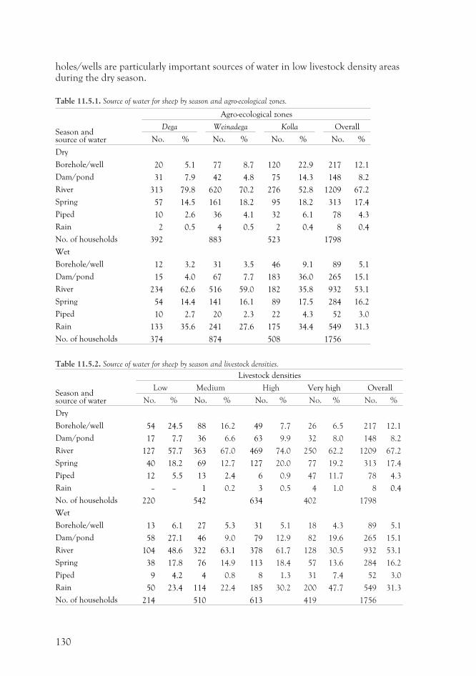
holes/wells are particularly important sources of water in low livestock density areasduring the dry season.
Table 11.5.1. Source of water for sheep by season and agro-ecological zones.
Season andsource of water
Agro-ecological zones
Dega Weinadega Kolla Overall
No. % No. % No. % No. %
Dry
Borehole/well 20 5.1 77 8.7 120 22.9 217 12.1
Dam/pond 31 7.9 42 4.8 75 14.3 148 8.2
River 313 79.8 620 70.2 276 52.8 1209 67.2
Spring 57 14.5 161 18.2 95 18.2 313 17.4
Piped 10 2.6 36 4.1 32 6.1 78 4.3
Rain 2 0.5 4 0.5 2 0.4 8 0.4
No. of households 392 883 523 1798
Wet
Borehole/well 12 3.2 31 3.5 46 9.1 89 5.1
Dam/pond 15 4.0 67 7.7 183 36.0 265 15.1
River 234 62.6 516 59.0 182 35.8 932 53.1
Spring 54 14.4 141 16.1 89 17.5 284 16.2
Piped 10 2.7 20 2.3 22 4.3 52 3.0
Rain 133 35.6 241 27.6 175 34.4 549 31.3
No. of households 374 874 508 1756
Table 11.5.2. Source of water for sheep by season and livestock densities.
Season andsource of water
Livestock densities
Low Medium High Very high Overall
No. % No. % No. % No. % No. %
Dry
Borehole/well 54 24.5 88 16.2 49 7.7 26 6.5 217 12.1
Dam/pond 17 7.7 36 6.6 63 9.9 32 8.0 148 8.2
River 127 57.7 363 67.0 469 74.0 250 62.2 1209 67.2
Spring 40 18.2 69 12.7 127 20.0 77 19.2 313 17.4
Piped 12 5.5 13 2.4 6 0.9 47 11.7 78 4.3
Rain – – 1 0.2 3 0.5 4 1.0 8 0.4
No. of households 220 542 634 402 1798
Wet
Borehole/well 13 6.1 27 5.3 31 5.1 18 4.3 89 5.1
Dam/pond 58 27.1 46 9.0 79 12.9 82 19.6 265 15.1
River 104 48.6 322 63.1 378 61.7 128 30.5 932 53.1
Spring 38 17.8 76 14.9 113 18.4 57 13.6 284 16.2
Piped 9 4.2 4 0.8 8 1.3 31 7.4 52 3.0
Rain 50 23.4 114 22.4 185 30.2 200 47.7 549 31.3
No. of households 214 510 613 419 1756
130
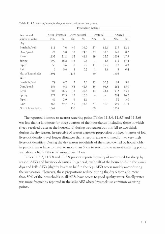
Table 11.5.3. Source of water for sheep by season and production systems.
Season and
source of water
Production systems
Crop–livestock Agro-pastoral Pastoral Overall
No. % No. % No. % No. %
Dry
Borehole/well 111 7.0 49 36.0 57 82.6 217 12.1
Dam/pond 92 5.8 33 24.3 23 33.3 148 8.2
River 1132 71.2 57 41.9 19 27.5 1208 67.3
Spring 299 18.8 13 9.6 1 1.4 313 17.4
Piped 58 3.6 8 5.9 11 15.9 77 4.3
Rain 6 0.4 1 0.7 1 1.4 8 0.4
No. of households 1591 136 69 1796
Wet
Borehole/well 74 4.7 3 2.3 12 20.7 89 5.1
Dam/pond 154 9.8 55 42.3 55 94.8 264 15.0
River 885 56.5 33 25.4 14 24.1 932 53.1
Spring 271 17.3 13 10.0 – – 284 16.2
Piped 46 2.9 6 4.6 – – 52 3.0
Rain 465 29.7 57 43.8 27 46.6 549 31.3
No. of households 1567 130 58 1755
The reported distance to nearest watering point (Tables 11.5.4, 11.5.5 and 11.5.6)
was less than a kilometre for three-quarters of the households (including those in which
sheep received water at the household) during wet season but this fell to two-thirds
during the dry season. Irrespective of season a greater proportion of sheep in areas of low
livestock density travel longer distances than sheep in areas with medium to very high
livestock densities. During the dry season two-thirds of the sheep owned by households
in pastoral areas have to travel to more than 5 km to reach to the nearest watering point,
and about a half of these, to more than 10 km.
Tables 11.5.7, 11.5.8 and 11.5.9 present reported quality of water used for sheep by
season, AEZs and livestock densities. In general, over half of the households in the weina-
dega and kolla AEZs (slightly less than half in the dega AEZ) access muddy water during
the wet season. However, these proportions reduce during the dry season and more
than 80% of the households in all AEZs have access to good quality water. Smelly water
was more frequently reported in the kolla AEZ where livestock use common watering
points.
131
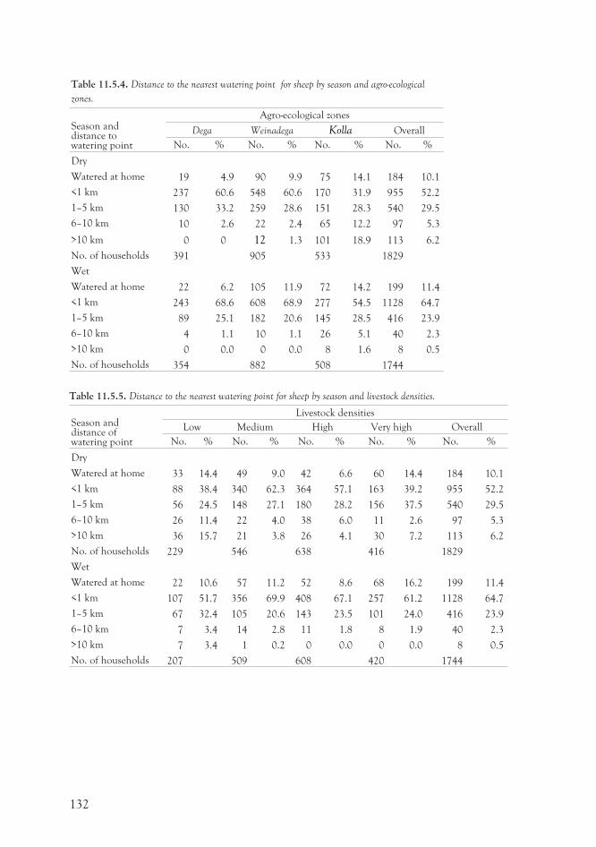
Table 11.5.4. Distance to the nearest watering point for sheep by season and agro-ecological
zones.
Season anddistance towatering point
Agro-ecological zones
Dega Weinadega Kolla Overall
No. % No. % No. % No. %
Dry
Watered at home 19 4.9 90 9.9 75 14.1 184 10.1
<1 km 237 60.6 548 60.6 170 31.9 955 52.2
1–5 km 130 33.2 259 28.6 151 28.3 540 29.5
6–10 km 10 2.6 22 2.4 65 12.2 97 5.3
>10 km 0 0 12 1.3 101 18.9 113 6.2
No. of households 391 905 533 1829
Wet
Watered at home 22 6.2 105 11.9 72 14.2 199 11.4
<1 km 243 68.6 608 68.9 277 54.5 1128 64.7
1–5 km 89 25.1 182 20.6 145 28.5 416 23.9
6–10 km 4 1.1 10 1.1 26 5.1 40 2.3
>10 km 0 0.0 0 0.0 8 1.6 8 0.5
No. of households 354 882 508 1744
Table 11.5.5. Distance to the nearest watering point for sheep by season and livestock densities.
Season anddistance ofwatering point
Livestock densities
Low Medium High Very high Overall
No. % No. % No. % No. % No. %
Dry
Watered at home 33 14.4 49 9.0 42 6.6 60 14.4 184 10.1
<1 km 88 38.4 340 62.3 364 57.1 163 39.2 955 52.2
1–5 km 56 24.5 148 27.1 180 28.2 156 37.5 540 29.5
6–10 km 26 11.4 22 4.0 38 6.0 11 2.6 97 5.3
>10 km 36 15.7 21 3.8 26 4.1 30 7.2 113 6.2
No. of households 229 546 638 416 1829
Wet
Watered at home 22 10.6 57 11.2 52 8.6 68 16.2 199 11.4
<1 km 107 51.7 356 69.9 408 67.1 257 61.2 1128 64.7
1–5 km 67 32.4 105 20.6 143 23.5 101 24.0 416 23.9
6–10 km 7 3.4 14 2.8 11 1.8 8 1.9 40 2.3
>10 km 7 3.4 1 0.2 0 0.0 0 0.0 8 0.5
No. of households 207 509 608 420 1744
132
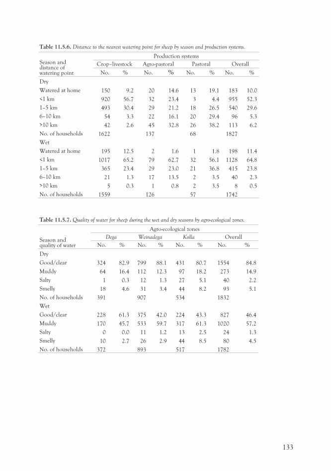
Table 11.5.6. Distance to the nearest watering point for sheep by season and production systems.
Season anddistance ofwatering point
Production systems
Crop–livestock Agro-pastoral Pastoral Overall
No. % No. % No. % No. %
Dry
Watered at home 150 9.2 20 14.6 13 19.1 183 10.0
<1 km 920 56.7 32 23.4 3 4.4 955 52.3
1–5 km 493 30.4 29 21.2 18 26.5 540 29.6
6–10 km 54 3.3 22 16.1 20 29.4 96 5.3
>10 km 42 2.6 45 32.8 26 38.2 113 6.2
No. of households 1622 137 68 1827
Wet
Watered at home 195 12.5 2 1.6 1 1.8 198 11.4
<1 km 1017 65.2 79 62.7 32 56.1 1128 64.8
1–5 km 365 23.4 29 23.0 21 36.8 415 23.8
6–10 km 21 1.3 17 13.5 2 3.5 40 2.3
>10 km 5 0.3 1 0.8 2 3.5 8 0.5
No. of households 1559 126 57 1742
Table 11.5.7. Quality of water for sheep during the wet and dry seasons by agro-ecological zones.
Season andquality of water
Agro-ecological zones
Dega Weinadega Kolla Overall
No. % No. % No. % No. %
Dry
Good/clear 324 82.9 799 88.1 431 80.7 1554 84.8
Muddy 64 16.4 112 12.3 97 18.2 273 14.9
Salty 1 0.3 12 1.3 27 5.1 40 2.2
Smelly 18 4.6 31 3.4 44 8.2 93 5.1
No. of households 391 907 534 1832
Wet
Good/clear 228 61.3 375 42.0 224 43.3 827 46.4
Muddy 170 45.7 533 59.7 317 61.3 1020 57.2
Salty 0 0.0 11 1.2 13 2.5 24 1.3
Smelly 10 2.7 26 2.9 44 8.5 80 4.5
No. of households 372 893 517 1782
133
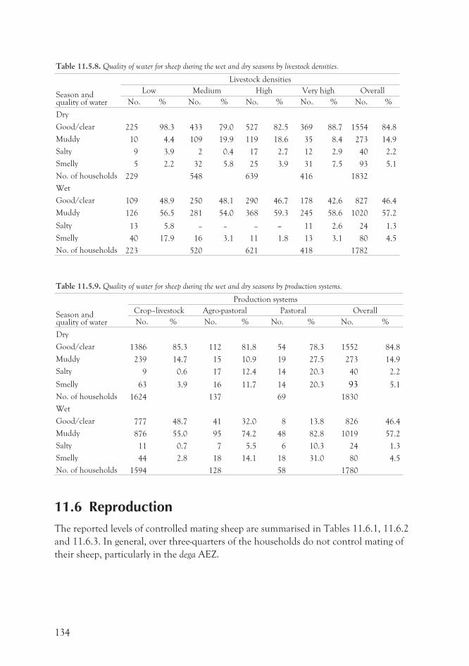
Table 11.5.8. Quality of water for sheep during the wet and dry seasons by livestock densities.
Season andquality of water
Livestock densities
Low Medium High Very high Overall
No. % No. % No. % No. % No. %
Dry
Good/clear 225 98.3 433 79.0 527 82.5 369 88.7 1554 84.8
Muddy 10 4.4 109 19.9 119 18.6 35 8.4 273 14.9
Salty 9 3.9 2 0.4 17 2.7 12 2.9 40 2.2
Smelly 5 2.2 32 5.8 25 3.9 31 7.5 93 5.1
No. of households 229 548 639 416 1832
Wet
Good/clear 109 48.9 250 48.1 290 46.7 178 42.6 827 46.4
Muddy 126 56.5 281 54.0 368 59.3 245 58.6 1020 57.2
Salty 13 5.8 – – – – 11 2.6 24 1.3
Smelly 40 17.9 16 3.1 11 1.8 13 3.1 80 4.5
No. of households 223 520 621 418 1782
Table 11.5.9. Quality of water for sheep during the wet and dry seasons by production systems.
Season andquality of water
Production systems
Crop–livestock Agro-pastoral Pastoral Overall
No. % No. % No. % No. %
Dry
Good/clear 1386 85.3 112 81.8 54 78.3 1552 84.8
Muddy 239 14.7 15 10.9 19 27.5 273 14.9
Salty 9 0.6 17 12.4 14 20.3 40 2.2
Smelly 63 3.9 16 11.7 14 20.3 93 5.1
No. of households 1624 137 69 1830
Wet
Good/clear 777 48.7 41 32.0 8 13.8 826 46.4
Muddy 876 55.0 95 74.2 48 82.8 1019 57.2
Salty 11 0.7 7 5.5 6 10.3 24 1.3
Smelly 44 2.8 18 14.1 18 31.0 80 4.5
No. of households 1594 128 58 1780
11.6 ReproductionThe reported levels of controlled mating sheep are summarised in Tables 11.6.1, 11.6.2
and 11.6.3. In general, over three-quarters of the households do not control mating of
their sheep, particularly in the dega AEZ.
134
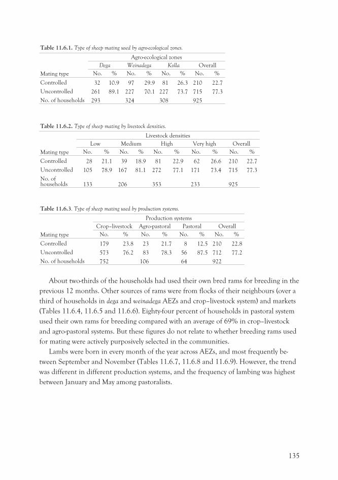
Table 11.6.1. Type of sheep mating used by agro-ecological zones.
Mating type
Agro-ecological zones
Dega Weinadega Kolla Overall
No. % No. % No. % No. %
Controlled 32 10.9 97 29.9 81 26.3 210 22.7
Uncontrolled 261 89.1 227 70.1 227 73.7 715 77.3
No. of households 293 324 308 925
Table 11.6.2. Type of sheep mating by livestock densities.
Mating type
Livestock densities
Low Medium High Very high Overall
No. % No. % No. % No. % No. %
Controlled 28 21.1 39 18.9 81 22.9 62 26.6 210 22.7
Uncontrolled 105 78.9 167 81.1 272 77.1 171 73.4 715 77.3
No. ofhouseholds 133 206 353 233 925
Table 11.6.3. Type of sheep mating used by production systems.
Mating type
Production systems
Crop–livestock Agro-pastoral Pastoral Overall
No. % No. % No. % No. %
Controlled 179 23.8 23 21.7 8 12.5 210 22.8
Uncontrolled 573 76.2 83 78.3 56 87.5 712 77.2
No. of households 752 106 64 922
About two-thirds of the households had used their own bred rams for breeding in the
previous 12 months. Other sources of rams were from flocks of their neighbours (over a
third of households in dega and weinadega AEZs and crop–livestock system) and markets
(Tables 11.6.4, 11.6.5 and 11.6.6). Eighty-four percent of households in pastoral system
used their own rams for breeding compared with an average of 69% in crop–livestock
and agro-pastoral systems. But these figures do not relate to whether breeding rams used
for mating were actively purposively selected in the communities.
Lambs were born in every month of the year across AEZs, and most frequently be-
tween September and November (Tables 11.6.7, 11.6.8 and 11.6.9). However, the trend
was different in different production systems, and the frequency of lambing was highest
between January and May among pastoralists.
135
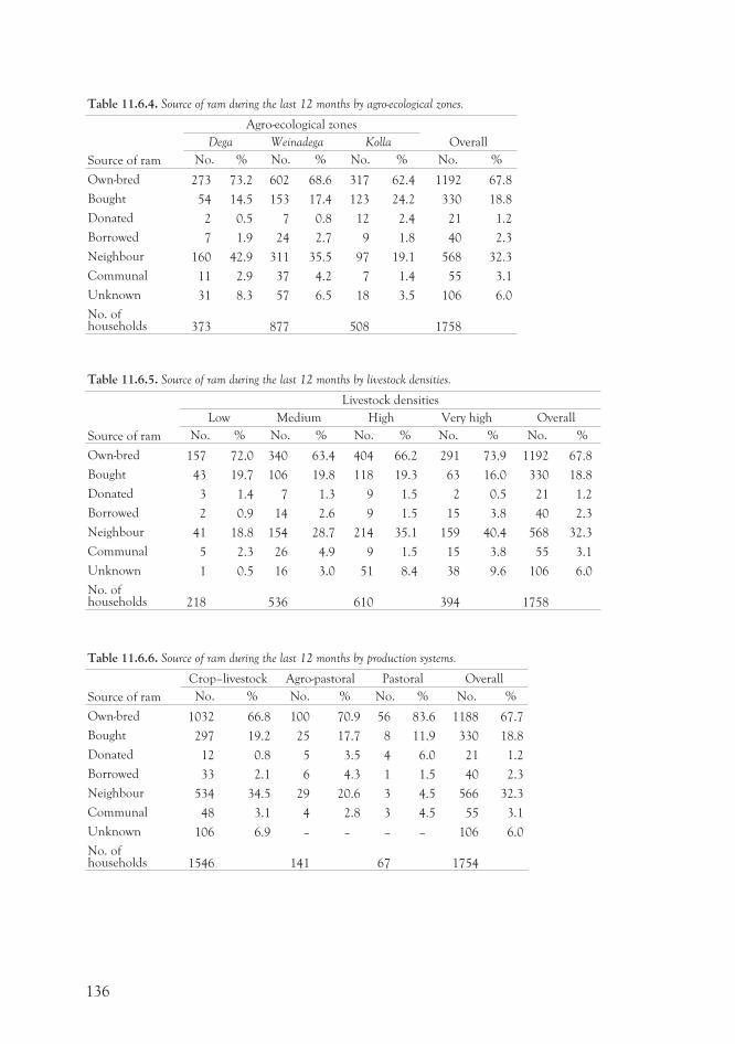
Table 11.6.4. Source of ram during the last 12 months by agro-ecological zones.
Source of ram
Agro-ecological zones
OverallDega Weinadega Kolla
No. % No. % No. % No. %
Own-bred 273 73.2 602 68.6 317 62.4 1192 67.8
Bought 54 14.5 153 17.4 123 24.2 330 18.8
Donated 2 0.5 7 0.8 12 2.4 21 1.2
Borrowed 7 1.9 24 2.7 9 1.8 40 2.3
Neighbour 160 42.9 311 35.5 97 19.1 568 32.3
Communal 11 2.9 37 4.2 7 1.4 55 3.1
Unknown 31 8.3 57 6.5 18 3.5 106 6.0
No. ofhouseholds 373 877 508 1758
Table 11.6.5. Source of ram during the last 12 months by livestock densities.
Source of ram
Livestock densities
Low Medium High Very high Overall
No. % No. % No. % No. % No. %
Own-bred 157 72.0 340 63.4 404 66.2 291 73.9 1192 67.8
Bought 43 19.7 106 19.8 118 19.3 63 16.0 330 18.8
Donated 3 1.4 7 1.3 9 1.5 2 0.5 21 1.2
Borrowed 2 0.9 14 2.6 9 1.5 15 3.8 40 2.3
Neighbour 41 18.8 154 28.7 214 35.1 159 40.4 568 32.3
Communal 5 2.3 26 4.9 9 1.5 15 3.8 55 3.1
Unknown 1 0.5 16 3.0 51 8.4 38 9.6 106 6.0
No. ofhouseholds 218 536 610 394 1758
Table 11.6.6. Source of ram during the last 12 months by production systems.
Source of ram
Crop–livestock Agro-pastoral Pastoral Overall
No. % No. % No. % No. %
Own-bred 1032 66.8 100 70.9 56 83.6 1188 67.7
Bought 297 19.2 25 17.7 8 11.9 330 18.8
Donated 12 0.8 5 3.5 4 6.0 21 1.2
Borrowed 33 2.1 6 4.3 1 1.5 40 2.3
Neighbour 534 34.5 29 20.6 3 4.5 566 32.3
Communal 48 3.1 4 2.8 3 4.5 55 3.1
Unknown 106 6.9 – – – – 106 6.0
No. ofhouseholds 1546 141 67 1754
136
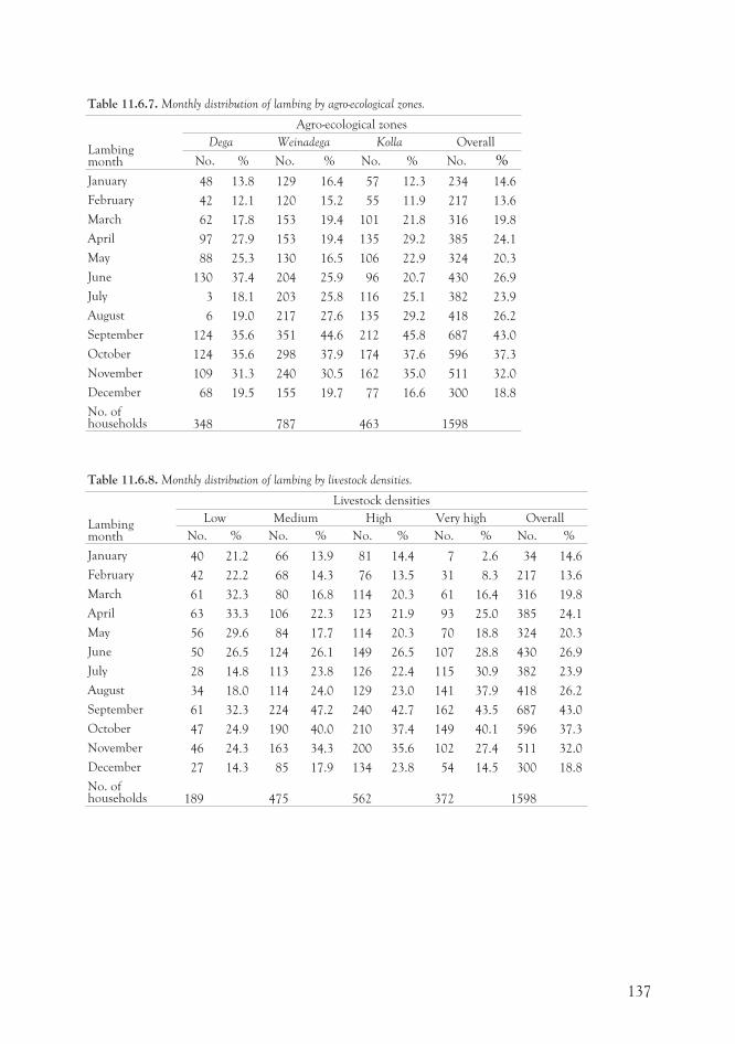
Table 11.6.7. Monthly distribution of lambing by agro-ecological zones.
Lambingmonth
Agro-ecological zones
Dega Weinadega Kolla Overall
No. % No. % No. % No. %
January 48 13.8 129 16.4 57 12.3 234 14.6
February 42 12.1 120 15.2 55 11.9 217 13.6
March 62 17.8 153 19.4 101 21.8 316 19.8
April 97 27.9 153 19.4 135 29.2 385 24.1
May 88 25.3 130 16.5 106 22.9 324 20.3
June 130 37.4 204 25.9 96 20.7 430 26.9
July 3 18.1 203 25.8 116 25.1 382 23.9
August 6 19.0 217 27.6 135 29.2 418 26.2
September 124 35.6 351 44.6 212 45.8 687 43.0
October 124 35.6 298 37.9 174 37.6 596 37.3
November 109 31.3 240 30.5 162 35.0 511 32.0
December 68 19.5 155 19.7 77 16.6 300 18.8
No. ofhouseholds 348 787 463 1598
Table 11.6.8. Monthly distribution of lambing by livestock densities.
Lambingmonth
Livestock densities
Low Medium High Very high Overall
No. % No. % No. % No. % No. %
January 40 21.2 66 13.9 81 14.4 7 2.6 34 14.6
February 42 22.2 68 14.3 76 13.5 31 8.3 217 13.6
March 61 32.3 80 16.8 114 20.3 61 16.4 316 19.8
April 63 33.3 106 22.3 123 21.9 93 25.0 385 24.1
May 56 29.6 84 17.7 114 20.3 70 18.8 324 20.3
June 50 26.5 124 26.1 149 26.5 107 28.8 430 26.9
July 28 14.8 113 23.8 126 22.4 115 30.9 382 23.9
August 34 18.0 114 24.0 129 23.0 141 37.9 418 26.2
September 61 32.3 224 47.2 240 42.7 162 43.5 687 43.0
October 47 24.9 190 40.0 210 37.4 149 40.1 596 37.3
November 46 24.3 163 34.3 200 35.6 102 27.4 511 32.0
December 27 14.3 85 17.9 134 23.8 54 14.5 300 18.8
No. ofhouseholds 189 475 562 372 1598
137
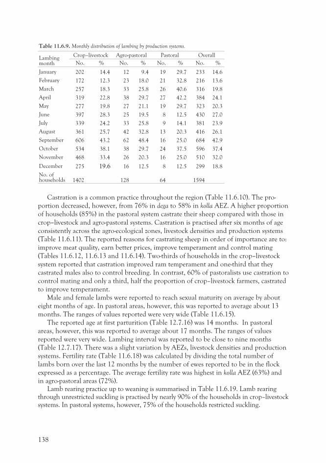
Table 11.6.9. Monthly distribution of lambing by production systems.
Lambingmonth
Crop–livestock Agro-pastoral Pastoral Overall
No. % No. % No. % No. %
January 202 14.4 12 9.4 19 29.7 233 14.6
February 172 12.3 23 18.0 21 32.8 216 13.6
March 257 18.3 33 25.8 26 40.6 316 19.8
April 319 22.8 38 29.7 27 42.2 384 24.1
May 277 19.8 27 21.1 19 29.7 323 20.3
June 397 28.3 25 19.5 8 12.5 430 27.0
July 339 24.2 33 25.8 9 14.1 381 23.9
August 361 25.7 42 32.8 13 20.3 416 26.1
September 606 43.2 62 48.4 16 25.0 684 42.9
October 534 38.1 38 29.7 24 37.5 596 37.4
November 468 33.4 26 20.3 16 25.0 510 32.0
December 275 19.6 16 12.5 8 12.5 299 18.8
No. ofhouseholds 1402 128 64 1594
Castration is a common practice throughout the region (Table 11.6.10). The pro-
portion decreased, however, from 76% in dega to 58% in kolla AEZ. A higher proportion
of households (85%) in the pastoral system castrate their sheep compared with those in
crop–livestock and agro-pastoral systems. Castration is practised after six months of age
consistently across the agro-ecological zones, livestock densities and production systems
(Table 11.6.11). The reported reasons for castrating sheep in order of importance are to:
improve meat quality, earn better prices, improve temperament and control mating
(Tables 11.6.12, 11.6.13 and 11.6.14). Two-thirds of households in the crop–livestock
system reported that castration improved ram temperament and one-third that they
castrated males also to control breeding. In contrast, 60% of pastoralists use castration to
control mating and only a third, half the proportion of crop–livestock farmers, castrated
to improve temperament.
Male and female lambs were reported to reach sexual maturity on average by about
eight months of age. In pastoral areas, however, this was reported to average about 13
months. The ranges of values reported were very wide (Table 11.6.15).
The reported age at first parturition (Table 12.7.16) was 14 months. In pastoral
areas, however, this was reported to average about 17 months. The ranges of values
reported were very wide. Lambing interval was reported to be close to nine months
(Table 12.7.17). There was a slight variation by AEZs, livestock densities and production
systems. Fertility rate (Table 11.6.18) was calculated by dividing the total number of
lambs born over the last 12 months by the number of ewes reported to be in the flock
expressed as a percentage. The average fertility rate was highest in kolla AEZ (63%) and
in agro-pastoral areas (72%).Lamb rearing practice up to weaning is summarised in Table 11.6.19. Lamb rearing
through unrestricted suckling is practised by nearly 90% of the households in crop–livestocksystems. In pastoral systems, however, 75% of the households restricted suckling.
138
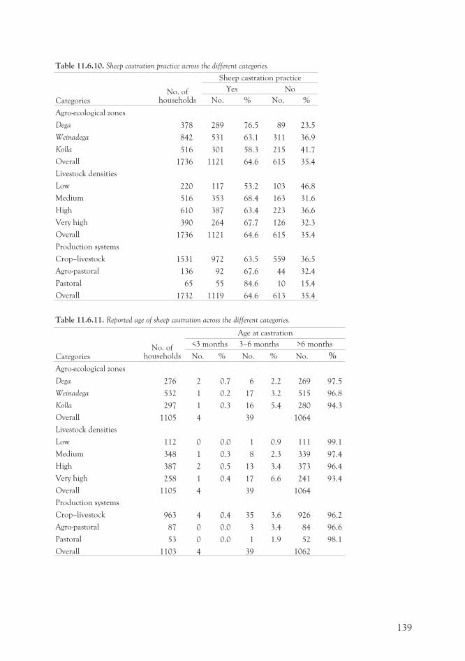
Table 11.6.10. Sheep castration practice across the different categories.
CategoriesNo. of
households
Sheep castration practice
Yes No
No. % No. %
Agro-ecological zones
Dega 378 289 76.5 89 23.5
Weinadega 842 531 63.1 311 36.9
Kolla 516 301 58.3 215 41.7
Overall 1736 1121 64.6 615 35.4
Livestock densities
Low 220 117 53.2 103 46.8
Medium 516 353 68.4 163 31.6
High 610 387 63.4 223 36.6
Very high 390 264 67.7 126 32.3
Overall 1736 1121 64.6 615 35.4
Production systems
Crop–livestock 1531 972 63.5 559 36.5
Agro-pastoral 136 92 67.6 44 32.4
Pastoral 65 55 84.6 10 15.4
Overall 1732 1119 64.6 613 35.4
Table 11.6.11. Reported age of sheep castration across the different categories.
CategoriesNo. of
households
Age at castration
<3 months 3–6 months >6 months
No. % No. % No. %
Agro-ecological zones
Dega 276 2 0.7 6 2.2 269 97.5
Weinadega 532 1 0.2 17 3.2 515 96.8
Kolla 297 1 0.3 16 5.4 280 94.3
Overall 1105 4 39 1064
Livestock densities
Low 112 0 0.0 1 0.9 111 99.1
Medium 348 1 0.3 8 2.3 339 97.4
High 387 2 0.5 13 3.4 373 96.4
Very high 258 1 0.4 17 6.6 241 93.4
Overall 1105 4 39 1064
Production systems
Crop–livestock 963 4 0.4 35 3.6 926 96.2
Agro-pastoral 87 0 0.0 3 3.4 84 96.6
Pastoral 53 0 0.0 1 1.9 52 98.1
Overall 1103 4 39 1062
139
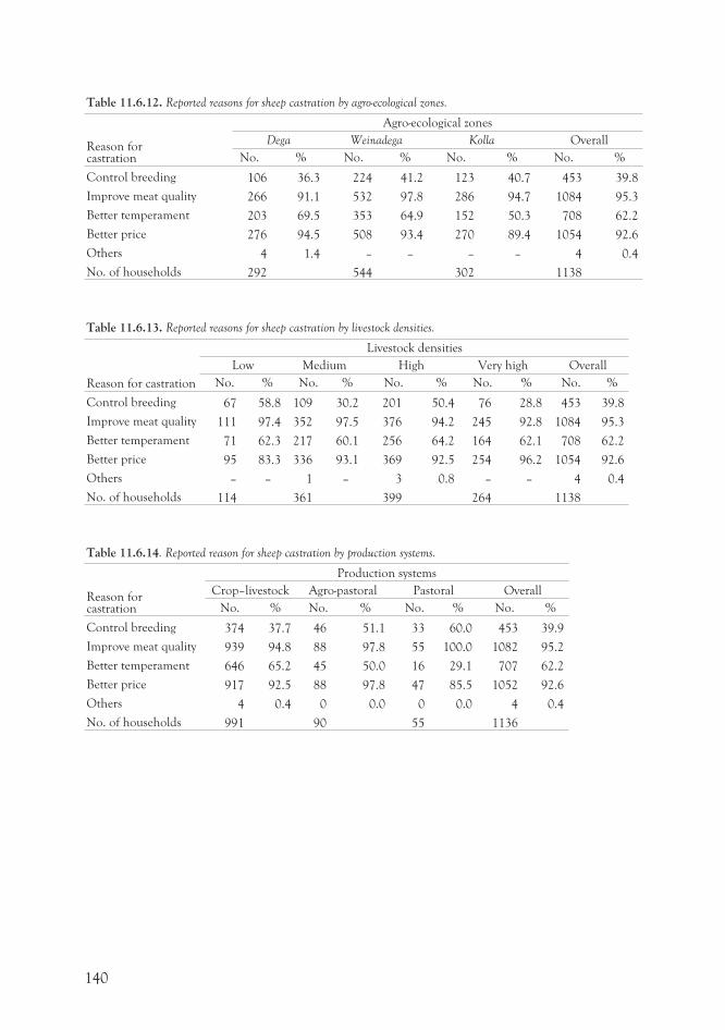
Table 11.6.12. Reported reasons for sheep castration by agro-ecological zones.
Reason forcastration
Agro-ecological zones
Dega Weinadega Kolla Overall
No. % No. % No. % No. %
Control breeding 106 36.3 224 41.2 123 40.7 453 39.8
Improve meat quality 266 91.1 532 97.8 286 94.7 1084 95.3
Better temperament 203 69.5 353 64.9 152 50.3 708 62.2
Better price 276 94.5 508 93.4 270 89.4 1054 92.6
Others 4 1.4 – – – – 4 0.4
No. of households 292 544 302 1138
Table 11.6.13. Reported reasons for sheep castration by livestock densities.
Reason for castration
Livestock densities
Low Medium High Very high Overall
No. % No. % No. % No. % No. %
Control breeding 67 58.8 109 30.2 201 50.4 76 28.8 453 39.8
Improve meat quality 111 97.4 352 97.5 376 94.2 245 92.8 1084 95.3
Better temperament 71 62.3 217 60.1 256 64.2 164 62.1 708 62.2
Better price 95 83.3 336 93.1 369 92.5 254 96.2 1054 92.6
Others – – 1 – 3 0.8 – – 4 0.4
No. of households 114 361 399 264 1138
Table 11.6.14. Reported reason for sheep castration by production systems.
Reason forcastration
Production systems
Crop–livestock Agro-pastoral Pastoral Overall
No. % No. % No. % No. %
Control breeding 374 37.7 46 51.1 33 60.0 453 39.9
Improve meat quality 939 94.8 88 97.8 55 100.0 1082 95.2
Better temperament 646 65.2 45 50.0 16 29.1 707 62.2
Better price 917 92.5 88 97.8 47 85.5 1052 92.6
Others 4 0.4 0 0.0 0 0.0 4 0.4
No. of households 991 90 55 1136
140
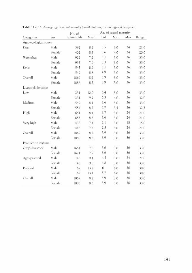
Table 11.6.15. Average age at sexual maturity (months) of sheep across different categories.
Categories SexNo. of
households
Age of sexual maturity
Mean Std Min Max Range
Agro-ecological zones
Dega Male 397 8.2 3.5 3.0 24 21.0
Female 402 8.3 3.6 4.0 24 20.0
Weinadega Male 927 7.7 3.1 3.0 36 33.0
Female 935 7.9 3.3 3.0 36 33.0
Kolla Male 545 8.9 5.1 3.0 36 33.0
Female 549 8.8 4.9 3.0 36 33.0
Overall Male 1869 8.2 3.9 3.0 36 33.0
Female 1886 8.3 3.9 3.0 36 33.0
Livestock densities
Low Male 231 10.0 6.4 3.0 36 33.0
Female 231 9.7 6.3 4.0 36 32.0
Medium Male 549 8.1 3.6 3.0 36 33.0
Female 554 8.2 3.7 3.5 36 32.5
High Male 651 8.1 3.7 3.0 24 21.0
Female 655 8.3 3.6 3.0 24 21.0
Very high Male 438 7.4 2.1 3.0 18 15.0
Female 446 7.5 2.5 3.0 24 21.0
Overall Male 1869 8.2 3.9 3.0 36 33.0
Female 1886 8.3 3.9 3.0 36 33.0
Production systems
Crop–livestock Male 1654 7.8 3.6 3.0 36 33.0
Female 1671 7.9 3.6 3.0 36 33.0
Agro-pastoral Male 146 9.4 4.5 3.0 24 21.0
Female 146 9.5 4.8 3.0 36 33.0
Pastoral Male 69 13.2 6 6.0 36 30.0
Female 69 13.1 5.7 6.0 36 30.0
Overall Male 1869 8.2 3.9 3.0 36 33.0
Female 1886 8.3 3.9 3.0 36 33.0
141
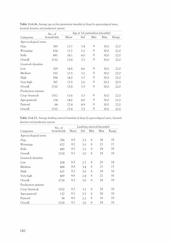
Table 11.6.16. Average age at first parturition (months) of sheep by agro-ecological zones,
livestock densities and production systems.
CategoriesNo. of
households
Age at 1st parturition (months)
Mean Std Min Max Range
Agro-ecological zones
Dega 385 13.7 3.4 8 30.0 22.0
Weinadega 834 13.7 3.2 8 30.0 22.0
Kolla 491 14.1 4.0 8 30.0 22.0
Overall 1710 13.8 3.5 8 30.0 22.0
Livestock densities
Low 209 14.8 4.6 8 30.0 22.0
Medium 510 13.5 3.2 8 30.0 22.0
High 594 14.0 3.7 8 30.0 22.0
Very high 397 13.5 2.6 8 28.5 20.5
Overall 1710 13.8 3.5 8 30.0 22.0
Production systems
Crop–livestock 1512 13.6 3.3 8 30.0 22.0
Agro-pastoral 134 14.6 4.0 9 30.0 21.0
Pastoral 64 17.4 4.9 8 30.0 22.0
Overall 1710 13.8 3.5 8 30.0 22.0
Table 11.6.17. Average lambing interval (months) of sheep by agro-ecological zones, livestock
densities and production systems.
CategoriesNo. of
households
Lambing interval (months)
Mean Std Min Max Range
Agro-ecological zones
Dega 356 8.9 2.5 6 24 18
Weinadega 872 9.2 3.0 6 23 17
Kolla 490 9.2 3.2 6 24 18
Overall 1718 9.2 3.0 6 24 18
Livestock densities
Low 204 8.5 2.7 6 20 14
Medium 484 9.8 3.4 6 23 17
High 621 9.2 3.0 6 24 18
Very high 409 8.6 2.4 6 22 16
Overall 1718 9.2 3.0 6 24 18
Production systems
Crop–livestock 1532 9.2 3.1 6 24 18
Agro-pastoral 132 9.1 2.5 6 24 18
Pastoral 54 8.6 2.2 6 16 10
Overall 1718 9.2 3.0 6 24 18
142
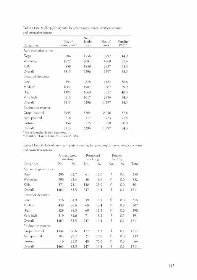
Table 11.6.18. Sheep fertility rates by agro-ecological zones, livestock densities
and production systems.
CategoriesNo. of
households*
No. oflambsborn
No. ofewes
Fertility(%)**
Agro-ecological zones
Dega 884 1756 3992 44.0
Weinadega 1572 2681 4668 57.4
Kolla 859 1859 2937 63.3
Overall 3315 6296 11597 54.3
Livestock densities
Low 393 828 1462 56.6
Medium 1002 1982 3307 59.9
High 1105 1869 3852 48.5
Very high 815 1617 2976 54.3
Overall 3315 6296 11,597 54.3
Production systems
Crop–livestock 2945 5264 10,016 52.6
Agro-pastoral 216 517 723 71.5
Pastoral 154 515 858 60.0
Overall 3315 6296 11,597 54.3
* No of households who have ewes.** Fertility = Lambs born/No. of ewes*100%.
Table 11.6.19. Type of lamb rearing up to weaning by agro-ecological zones, livestock densities
and production systems.
Categories
Unrestrictedsuckling
Restrictedsuckling
Bucketfeeding
TotalNo. % No. % No. %
Agro-ecological zones
Dega 296 82.7 61 17.0 1 0.3 358
Weinadega 796 93.4 56 6.6 0 0.0 852
Kolla 371 74.1 130 25.9 0 0.0 501
Overall 1463 85.5 247 14.4 1 0.1 1711
Livestock densities
Low 176 81.9 39 18.1 0 0.0 215
Medium 439 86.6 68 13.4 0 0.0 507
High 529 88.5 69 11.5 0 0.0 598
Very high 319 81.6 71 18.2 1 0.3 391
Overall 1463 85.5 247 14.4 1 0.1 1711
Production systems
Crop–livestock 1344 88.6 172 11.3 1 0.1 1517
Agro-pastoral 103 79.2 27 20.8 0 0.0 130
Pastoral 16 25.0 48 75.0 0 0.0 64
Overall 1463 85.5 247 14.4 1 0.1 1711
143
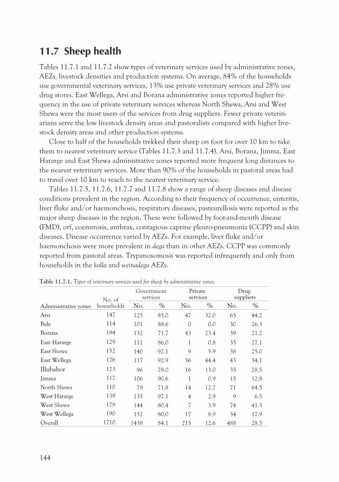
11.7 Sheep healthTables 11.7.1 and 11.7.2 show types of veterinary services used by administrative zones,
AEZs, livestock densities and production systems. On average, 84% of the households
use governmental veterinary services, 13% use private veterinary services and 28% use
drug stores. East Wellega, Arsi and Borana administrative zones reported higher fre-
quency in the use of private veterinary services whereas North Shewa, Arsi and West
Shewa were the most users of the services from drug suppliers. Fewer private veterin-
arians serve the low livestock density areas and pastoralists compared with higher live-
stock density areas and other production systems.
Close to half of the households trekked their sheep on foot for over 10 km to take
them to nearest veterinary service (Tables 11.7.3 and 11.7.4). Arsi, Borana, Jimma, East
Hararge and East Shewa administrative zones reported more frequent long distances to
the nearest veterinary services. More than 90% of the households in pastoral areas had
to travel over 10 km to reach to the nearest veterinary service.
Tables 11.7.5, 11.7.6, 11.7.7 and 11.7.8 show a range of sheep diseases and disease
conditions prevalent in the region. According to their frequency of occurrence, enteritis,
liver fluke and/or haemonchosis, respiratory diseases, pasteurellosis were reported as the
major sheep diseases in the region. These were followed by foot-and-mouth disease
(FMD), orf, coenurosis, anthrax, contagious caprine pleuro-pneumonia (CCPP) and skin
diseases. Disease occurrence varied by AEZs. For example, liver fluke and/or
haemonchosis were more prevalent in dega than in other AEZs. CCPP was commonly
reported from pastoral areas. Trypanosomosis was reported infrequently and only from
households in the kolla and weinadega AEZs.
Table 11.7.1. Types of veterinary services used for sheep by administrative zones.
Administrative zonesNo. of
households
Governmentservices
Privateservices
Drugsuppliers
No. % No. % No. %
Arsi 147 125 85.0 47 32.0 65 44.2
Bale 114 101 88.6 0 0.0 30 26.3
Borana 184 132 71.7 43 23.4 39 21.2
East Hararge 129 111 86.0 1 0.8 35 27.1
East Shewa 152 140 92.1 9 5.9 38 25.0
East Wellega 126 117 92.9 56 44.4 43 34.1
Illubabor 123 96 78.0 16 13.0 35 28.5
Jimma 117 106 90.6 1 0.9 15 12.8
North Shewa 110 79 71.8 14 12.7 71 64.5
West Hararge 139 135 97.1 4 2.9 9 6.5
West Shewa 179 144 80.4 7 3.9 74 41.3
West Wellega 190 152 80.0 17 8.9 34 17.9
Overall 1710 1438 84.1 215 12.6 488 28.5
144
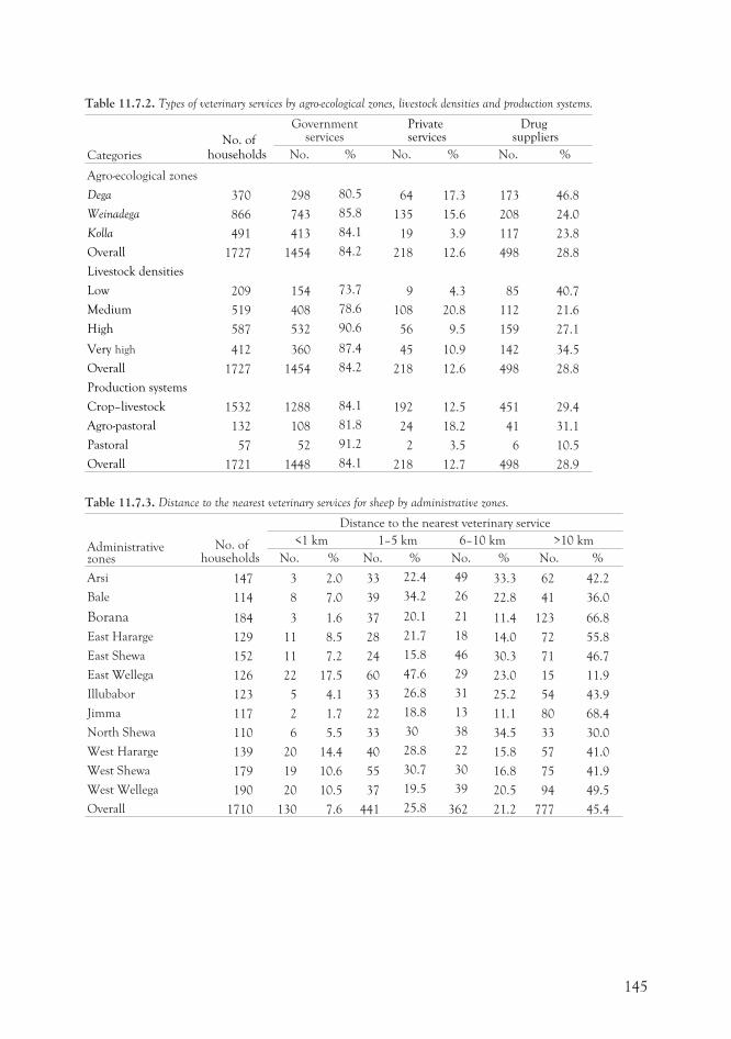
Table 11.7.2. Types of veterinary services by agro-ecological zones, livestock densities and production systems.
Categories
No. ofhouseholds
Governmentservices
Privateservices
Drugsuppliers
No. % No. % No. %
Agro-ecological zones
Dega 370 298 80.5 64 17.3 173 46.8
Weinadega 866 743 85.8 135 15.6 208 24.0
Kolla 491 413 84.1 19 3.9 117 23.8
Overall 1727 1454 84.2 218 12.6 498 28.8
Livestock densities
Low 209 154 73.7 9 4.3 85 40.7
Medium 519 408 78.6 108 20.8 112 21.6
High 587 532 90.6 56 9.5 159 27.1
Very high 412 360 87.4 45 10.9 142 34.5
Overall 1727 1454 84.2 218 12.6 498 28.8
Production systems
Crop–livestock 1532 1288 84.1 192 12.5 451 29.4
Agro-pastoral 132 108 81.8 24 18.2 41 31.1
Pastoral 57 52 91.2 2 3.5 6 10.5
Overall 1721 1448 84.1 218 12.7 498 28.9
Table 11.7.3. Distance to the nearest veterinary services for sheep by administrative zones.
Administrativezones
No. ofhouseholds
Distance to the nearest veterinary service
<1 km 1–5 km 6–10 km >10 km
No. % No. % No. % No. %
Arsi 147 3 2.0 33 22.4 49 33.3 62 42.2
Bale 114 8 7.0 39 34.2 26 22.8 41 36.0
Borana 184 3 1.6 37 20.1 21 11.4 123 66.8
East Hararge 129 11 8.5 28 21.7 18 14.0 72 55.8
East Shewa 152 11 7.2 24 15.8 46 30.3 71 46.7
East Wellega 126 22 17.5 60 47.6 29 23.0 15 11.9
Illubabor 123 5 4.1 33 26.8 31 25.2 54 43.9
Jimma 117 2 1.7 22 18.8 13 11.1 80 68.4
North Shewa 110 6 5.5 33 30 38 34.5 33 30.0
West Hararge 139 20 14.4 40 28.8 22 15.8 57 41.0
West Shewa 179 19 10.6 55 30.7 30 16.8 75 41.9
West Wellega 190 20 10.5 37 19.5 39 20.5 94 49.5
Overall 1710 130 7.6 441 25.8 362 21.2 777 45.4
145
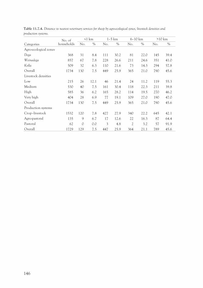
Table 11.7.4. Distance to nearest veterinary services for sheep by agro-ecological zones, livestock densities and
production systems.
CategoriesNo. of
households
<1 km 1–5 km 6–10 km >10 km
No. % No. % No. % No. %
Agro-ecological zones
Dega 368 31 8.4 111 30.2 81 22.0 145 39.4
Weinadega 857 67 7.8 228 26.6 211 24.6 351 41.0
Kolla 509 32 6.3 110 21.6 73 14.3 294 57.8
Overall 1734 130 7.5 449 25.9 365 21.0 790 45.6
Livestock densities
Low 215 26 12.1 46 21.4 24 11.2 119 55.3
Medium 530 40 7.5 161 30.4 118 22.3 211 39.8
High 585 36 6.2 165 28.2 114 19.5 270 46.2
Very high 404 28 6.9 77 19.1 109 27.0 190 47.0
Overall 1734 130 7.5 449 25.9 365 21.0 790 45.6
Production systems
Crop–livestock 1532 120 7.8 427 27.9 340 22.2 645 42.1
Agro-pastoral 135 9 6.7 17 12.6 22 16.3 87 64.4
Pastoral 62 0 0.0 3 4.8 2 3.2 57 91.9
Overall 1729 129 7.5 447 25.9 364 21.1 789 45.6
146
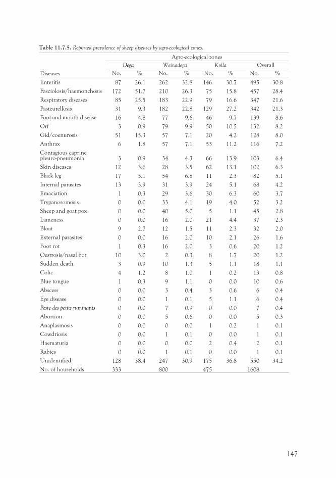
Table 11.7.5. Reported prevalence of sheep diseases by agro-ecological zones.
Diseases
Agro-ecological zones
Dega Weinadega Kolla Overall
No. % No. % No. % No. %
Enteritis 87 26.1 262 32.8 146 30.7 495 30.8
Fasciolosis/haemonchosis 172 51.7 210 26.3 75 15.8 457 28.4
Respiratory diseases 85 25.5 183 22.9 79 16.6 347 21.6
Pasteurellosis 31 9.3 182 22.8 129 27.2 342 21.3
Foot-and-mouth disease 16 4.8 77 9.6 46 9.7 139 8.6
Orf 3 0.9 79 9.9 50 10.5 132 8.2
Gid/coenurosis 51 15.3 57 7.1 20 4.2 128 8.0
Anthrax 6 1.8 57 7.1 53 11.2 116 7.2
Contagious caprinepleuro-pneumonia 3 0.9 34 4.3 66 13.9 103 6.4
Skin diseases 12 3.6 28 3.5 62 13.1 102 6.3
Black leg 17 5.1 54 6.8 11 2.3 82 5.1
Internal parasites 13 3.9 31 3.9 24 5.1 68 4.2
Emaciation 1 0.3 29 3.6 30 6.3 60 3.7
Trypanosomosis 0 0.0 33 4.1 19 4.0 52 3.2
Sheep and goat pox 0 0.0 40 5.0 5 1.1 45 2.8
Lameness 0 0.0 16 2.0 21 4.4 37 2.3
Bloat 9 2.7 12 1.5 11 2.3 32 2.0
External parasites 0 0.0 16 2.0 10 2.1 26 1.6
Foot rot 1 0.3 16 2.0 3 0.6 20 1.2
Oestrosis/nasal bot 10 3.0 2 0.3 8 1.7 20 1.2
Sudden death 3 0.9 10 1.3 5 1.1 18 1.1
Colic 4 1.2 8 1.0 1 0.2 13 0.8
Blue tongue 1 0.3 9 1.1 0 0.0 10 0.6
Abscess 0 0.0 3 0.4 3 0.6 6 0.4
Eye disease 0 0.0 1 0.1 5 1.1 6 0.4
Peste des petits ruminants 0 0.0 7 0.9 0 0.0 7 0.4
Abortion 0 0.0 5 0.6 0 0.0 5 0.3
Anaplasmosis 0 0.0 0 0.0 1 0.2 1 0.1
Cowdriosis 0 0.0 1 0.1 0 0.0 1 0.1
Haematuria 0 0.0 0 0.0 2 0.4 2 0.1
Rabies 0 0.0 1 0.1 0 0.0 1 0.1
Unidentified 128 38.4 247 30.9 175 36.8 550 34.2
No. of households 333 800 475 1608
147
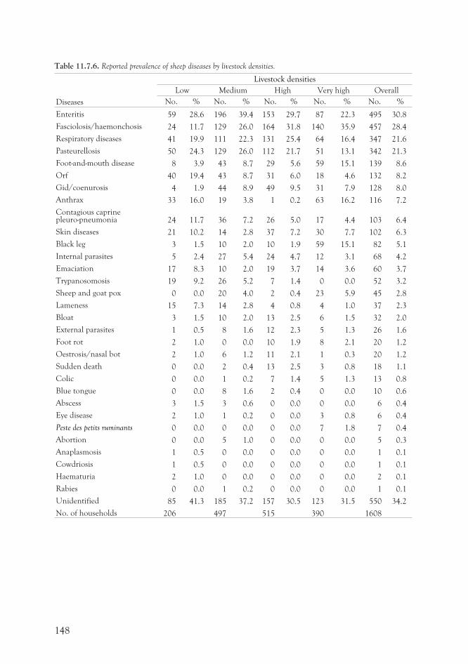
Table 11.7.6. Reported prevalence of sheep diseases by livestock densities.
Diseases
Livestock densities
Low Medium High Very high Overall
No. % No. % No. % No. % No. %
Enteritis 59 28.6 196 39.4 153 29.7 87 22.3 495 30.8
Fasciolosis/haemonchosis 24 11.7 129 26.0 164 31.8 140 35.9 457 28.4
Respiratory diseases 41 19.9 111 22.3 131 25.4 64 16.4 347 21.6
Pasteurellosis 50 24.3 129 26.0 112 21.7 51 13.1 342 21.3
Foot-and-mouth disease 8 3.9 43 8.7 29 5.6 59 15.1 139 8.6
Orf 40 19.4 43 8.7 31 6.0 18 4.6 132 8.2
Gid/coenurosis 4 1.9 44 8.9 49 9.5 31 7.9 128 8.0
Anthrax 33 16.0 19 3.8 1 0.2 63 16.2 116 7.2
Contagious caprinepleuro-pneumonia 24 11.7 36 7.2 26 5.0 17 4.4 103 6.4
Skin diseases 21 10.2 14 2.8 37 7.2 30 7.7 102 6.3
Black leg 3 1.5 10 2.0 10 1.9 59 15.1 82 5.1
Internal parasites 5 2.4 27 5.4 24 4.7 12 3.1 68 4.2
Emaciation 17 8.3 10 2.0 19 3.7 14 3.6 60 3.7
Trypanosomosis 19 9.2 26 5.2 7 1.4 0 0.0 52 3.2
Sheep and goat pox 0 0.0 20 4.0 2 0.4 23 5.9 45 2.8
Lameness 15 7.3 14 2.8 4 0.8 4 1.0 37 2.3
Bloat 3 1.5 10 2.0 13 2.5 6 1.5 32 2.0
External parasites 1 0.5 8 1.6 12 2.3 5 1.3 26 1.6
Foot rot 2 1.0 0 0.0 10 1.9 8 2.1 20 1.2
Oestrosis/nasal bot 2 1.0 6 1.2 11 2.1 1 0.3 20 1.2
Sudden death 0 0.0 2 0.4 13 2.5 3 0.8 18 1.1
Colic 0 0.0 1 0.2 7 1.4 5 1.3 13 0.8
Blue tongue 0 0.0 8 1.6 2 0.4 0 0.0 10 0.6
Abscess 3 1.5 3 0.6 0 0.0 0 0.0 6 0.4
Eye disease 2 1.0 1 0.2 0 0.0 3 0.8 6 0.4
Peste des petits ruminants 0 0.0 0 0.0 0 0.0 7 1.8 7 0.4
Abortion 0 0.0 5 1.0 0 0.0 0 0.0 5 0.3
Anaplasmosis 1 0.5 0 0.0 0 0.0 0 0.0 1 0.1
Cowdriosis 1 0.5 0 0.0 0 0.0 0 0.0 1 0.1
Haematuria 2 1.0 0 0.0 0 0.0 0 0.0 2 0.1
Rabies 0 0.0 1 0.2 0 0.0 0 0.0 1 0.1
Unidentified 85 41.3 185 37.2 157 30.5 123 31.5 550 34.2
No. of households 206 497 515 390 1608
148
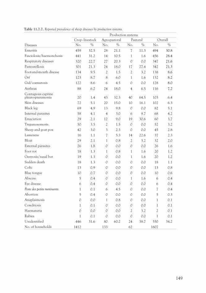
Table 11.7.7. Reported prevalence of sheep diseases by production systems.
Diseases
Production systems
Crop–livestock Agro-pastoral Pastoral Overall
No. % No. % No. % No. %
Enteritis 459 32.5 28 21.1 7 11.3 494 30.8
Fasciolosis/haemonchosis 441 31.2 14 10.5 1 1.6 456 28.4
Respiratory diseases 320 22.7 27 20.3 0 0.0 347 21.6
Pasteurellosis 301 21.3 24 18.0 17 27.4 342 21.3
Foot-and-mouth disease 134 9.5 2 1.5 2 3.2 138 8.6
Orf 123 8.7 8 6.0 1 1.6 132 8.2
Gid/coenurosis 122 8.6 6 4.5 0 0.0 128 8.0
Anthrax 88 6.2 24 18.0 4 6.5 116 7.2
Contagious caprinepleuro-pneumonia 20 1.4 43 32.3 40 64.5 103 6.4
Skin diseases 72 5.1 20 15.0 10 16.1 102 6.3
Black leg 69 4.9 13 9.8 0 0.0 82 5.1
Internal parasites 58 4.1 4 3.0 6 9.7 68 4.2
Emaciation 29 2.1 12 9.0 19 30.6 60 3.7
Trypanosomosis 50 3.5 2 1.5 0 0.0 52 3.2
Sheep and goat pox 42 3.0 3 2.3 0 0.0 45 2.8
Lameness 16 1.1 7 5.3 14 22.6 37 2.3
Bloat 29 2.1 1 0.8 2 3.2 32 2.0
External parasites 26 1.8 0 0.0 0 0.0 26 1.6
Foot rot 18 1.3 1 0.8 1 1.6 20 1.2
Oestrosis/nasal bot 19 1.3 0 0.0 1 1.6 20 1.2
Sudden death 18 1.3 0 0.0 0 0.0 18 1.1
Colic 13 0.9 0 0.0 0 0.0 13 0.8
Blue tongue 10 0.7 0 0.0 0 0.0 10 0.6
Abscess 5 0.4 0 0.0 1 1.6 6 0.4
Eye disease 6 0.4 0 0.0 0 0.0 6 0.4
Peste des petits ruminants 1 0.1 6 4.5 0 0.0 7 0.4
Abortion 5 0.4 0 0.0 0 0.0 5 0.3
Anaplasmosis 0 0.0 1 0.8 0 0.0 1 0.1
Cowdriosis 1 0.1 0 0.0 0 0.0 1 0.1
Haematuria 0 0.0 0 0.0 2 3.2 2 0.1
Rabies 1 0.1 0 0.0 0 0.0 1 0.1
Unidentified 446 31.6 80 60.2 24 38.7 550 34.2
No. of households 1412 133 62 1607
149
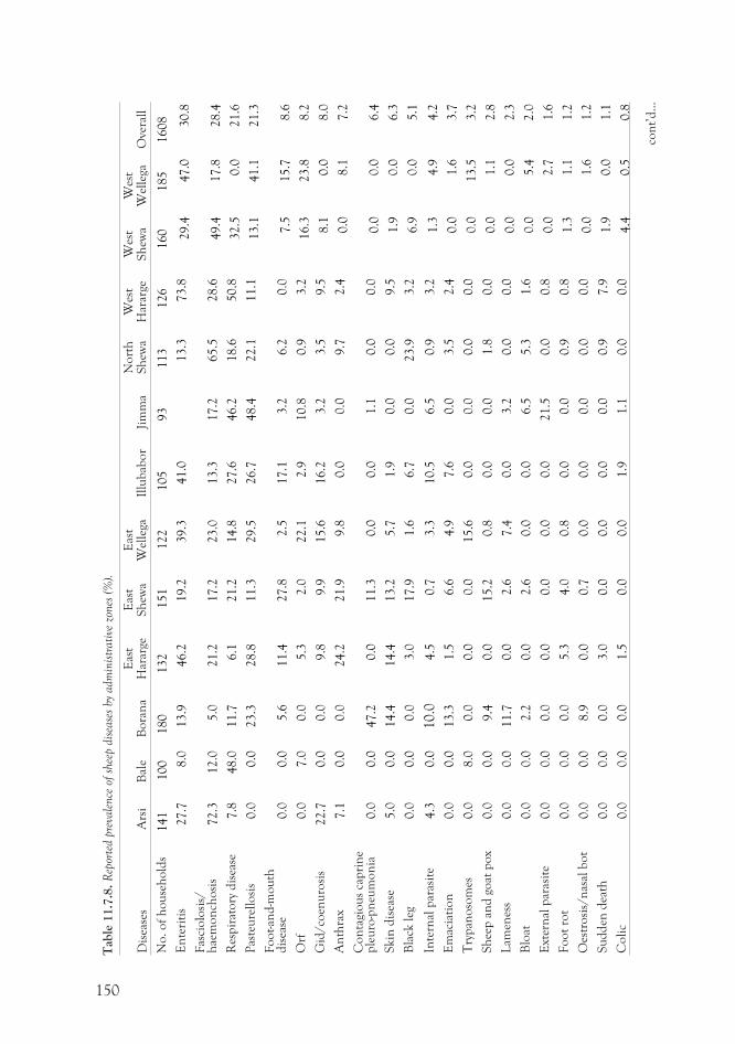
150
Tab
le11.7
.8.
Rep
orte
dpr
evale
nce
ofsh
eep
dise
ase
sby
adm
inis
trati
vezo
nes
(%).
Dis
ease
sA
rsi
Bal
eB
ora
na
Eas
tH
arar
geE
ast
Sh
ewa
Eas
tW
elle
gaIl
lub
abo
rJi
mm
aN
ort
hS
hew
aW
est
Har
arge
Wes
tS
hew
aW
est
Wel
lega
Ove
rall
No
.o
fh
ou
seh
old
s141
100
180
132
151
122
105
93
113
126
160
185
1608
En
teri
tis
27.7
8.0
13.9
46.2
19.2
39.3
41.0
13.3
73.8
29.4
47.0
30.8
Fas
cio
losi
s/h
aem
on
cho
sis
72.3
12.0
5.0
21.2
17.2
23
.013.3
17.2
65.5
28.6
49.4
17.8
28.4
Res
pir
ato
ryd
isea
se7.8
48.0
11.7
6.1
21.2
14.8
27.6
46.2
18.6
50.8
32.5
0.0
21.6
Pas
teu
rell
osi
s0.0
0.0
23.3
28.8
11.3
29.5
26.7
48.4
22.1
11.1
13.1
41.1
21.3
Fo
ot-an
d-m
ou
thd
isea
se0.0
0.0
5.6
11.4
27.8
2.5
17.1
3.2
6.2
0.0
7.5
15.7
8.6
Orf
0.0
7.0
0.0
5.3
2.0
22.1
2.9
10.8
0.9
3.2
16.3
23.8
8.2
Gid
/co
enu
rosi
s22.7
0.0
0.0
9.8
9.9
15.6
16.2
3.2
3.5
9.5
8.1
0.0
8.0
An
thra
x7.1
0.0
0.0
24.2
21.9
9.8
0.0
0.0
9.7
2.4
0.0
8.1
7.2
Co
nta
gio
us
cap
rin
ep
leu
ro-p
neu
mo
nia
0.0
0.0
47.2
0.0
11.3
0.0
0.0
1.1
0.0
0.0
0.0
0.0
6.4
Skin
dis
ease
5.0
0.0
14.4
14.4
13.2
5.7
1.9
0.0
0.0
9.5
1.9
0.0
6.3
Bla
ckle
g0.0
0.0
0.0
3.0
17.9
1.6
6.7
0.0
23.9
3.2
6.9
0.0
5.1
Inte
rnal
par
asit
e4.3
0.0
10.0
4.5
0.7
3.3
10.5
6.5
0.9
3.2
1.3
4.9
4.2
Em
acia
tio
n0.0
0.0
13.3
1.5
6.6
4.9
7.6
0.0
3.5
2.4
0.0
1.6
3.7
Try
pan
oso
mes
0.0
8.0
0.0
0.0
0.0
15.6
0.0
0.0
0.0
0.0
0.0
13.5
3.2
Sh
eep
and
goat
po
x0.0
0.0
9.4
0.0
15.2
0.8
0.0
0.0
1.8
0.0
0.0
1.1
2.8
Lam
enes
s0.0
0.0
11.7
0.0
2.6
7.4
0.0
3.2
0.0
0.0
0.0
0.0
2.3
Blo
at0.0
0.0
2.2
0.0
2.6
0.0
0.0
6.5
5.3
1.6
0.0
5.4
2.0
Ext
ern
alp
aras
ite
0.0
0.0
0.0
0.0
0.0
0.0
0.0
21.5
0.0
0.8
0.0
2.7
1.6
Fo
ot
rot
0.0
0.0
0.0
5.3
4.0
0.8
0.0
0.0
0.9
0.8
1.3
1.1
1.2
Oes
tro
sis/
nas
alb
ot
0.0
0.0
8.9
0.0
0.7
0.0
0.0
0.0
0.0
0.0
0.0
1.6
1.2
Su
dd
end
eath
0.0
0.0
0.0
3.0
0.0
0.0
0.0
0.0
0.9
7.9
1.9
0.0
1.1
Co
lic
0.0
0.0
0.0
1.5
0.0
0.0
1.9
1.1
0.0
0.0
4.4
0.5
0.8
con
t’d
...
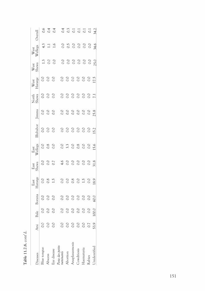
151
Dis
ease
sA
rsi
Bal
eB
ora
na
Eas
tH
arar
geE
ast
Sh
ewa
Eas
tW
elle
gaIl
lub
abo
rJi
mm
aN
ort
hS
hew
aW
est
Har
arge
Wes
tS
hew
aW
est
Wel
lega
Ove
rall
Blu
eto
ngu
e0.0
0.0
0.0
0.0
0.0
0.0
0.0
0.0
0.0
0.0
1.3
4.3
0.6
Ab
sces
s0.0
0.0
0.0
0.8
0.0
0.8
0.0
0.0
0.0
0.0
0.0
1.1
0.4
Eye
dis
ease
0.0
0.0
0.0
1.5
0.7
0.0
0.0
0.0
0.0
0.0
0.0
1.6
0.4
Pes
tedes
pet
its
rum
inants
0.0
0.0
0.0
0.0
4.6
0.0
0.0
0.0
0.0
0.0
0.0
0.0
0.4
Ab
ort
ion
0.0
0.0
0.0
0.0
0.0
3.3
0.0
0.0
0.0
0.0
0.0
0.5
0.3
An
apla
sasm
osi
s0.0
0.0
0.0
0.8
0.0
0.0
0.0
0.0
0.0
0.0
0.0
0.0
0.1
Co
wd
rio
sis
0.0
0.0
0.0
0.0
0.0
0.8
0.0
0.0
0.0
0.0
0.0
0.0
0.1
Hae
mat
uri
a0.0
0.0
0.0
1.5
0.0
0.0
0.0
0.0
0.0
0.0
0.0
0.0
0.1
Rab
ies
0.7
0.0
0.0
0.0
0.0
0.0
0.0
0.0
0.0
0.0
0.0
0.0
0.1
Un
iden
tifi
ed53.9
100.0
60.0
18.9
31.8
15.6
15.2
25.8
7.1
17.5
25.0
34.6
34.2
Tab
le11.7
.8.
con
t’d
.
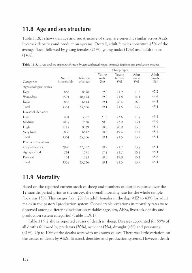
11.8 Age and sex structure
Table 11.8.1 shows that age and sex structure of sheep are generally similar across AEZs,
livestock densities and production systems. Overall, adult females constitute 45% of the
average flock, followed by young females (21%), young males (19%) and adult males
(14%).
Table 11.8.1. Age and sex structure of sheep by agro-ecological zones, livestock densities and production systems.
CategoriesNo. of
households
Sheep types
Total no.of sheep
Youngmale(%)
Youngfemale
(%)
Adutmale(%)
Adultfemale
(%)
Agro-ecological zones
Dega 888 8478 19.0 21.9 11.8 47.2
Weinadega 1591 10,474 19.2 21.8 14.4 44.6
Kolla 885 6614 19.1 20.4 16.0 44.5
Total 3364 25,566 19.1 21.5 13.9 45.4
Livestock densities
Low 404 3387 21.5 23.6 11.7 43.2
Medium 1037 7538 20.0 23.0 13.1 43.9
High 1117 8029 18.0 20.9 13.0 48.1
Very high 806 6612 18.3 19.4 17.2 45.1
Total 3364 25,566 19.1 21.5 13.9 45.4
Production systems
Crop–livestock 2990 22,062 19.2 21.7 13.7 45.4
Agro-pastoral 214 1591 17.7 21.2 15.7 45.4
Pastoral 154 1873 19.3 19.8 15.1 45.8
Total 3358 25,526 19.1 21.5 13.9 45.4
11.9 Mortality
Based on the reported current stock of sheep and numbers of deaths reported over the
12 months period prior to the survey, the overall mortality rate for the whole sample
flock was 15%. This ranges from 7% for adult females in the dega AEZ to 40% for adult
males in the pastoral production system. Considerable variations in mortality rates were
observed among different classification variables (age, sex, AEZs, livestock density and
production system categories) (Table 11.9.1).
Table 11.9.2 shows reported causes of death in sheep. Diseases accounted for 59% of
all deaths followed by predators (20%), accident (7%), drought (4%) and poisoning
(<1%). Up to 10% of the deaths were with unknown causes. There was little variation on
the causes of death by AEZs, livestock densities and production systems. However, death
152
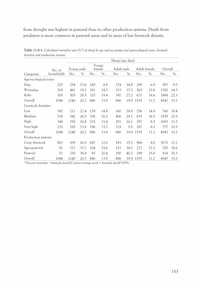
from drought was highest in pastoral than in other production systems. Death from
predators is more common in pastoral areas and in areas of low livestock density.
Table 11.9.1. Calculated mortality rate (%*) of sheep by age and sex groups and agro-ecological zones, livestock
densities and production systems.
Categories
Sheep type dead
No. ofhouseholds
Young maleYoungfemale Adult male Adult female Overall
No. % No. % No. % No. % No. %
Agro-ecological zones
Dega 220 254 13.6 180 8.8 174 14.8 299 6.9 907 9.7
Weinadega 519 481 19.3 381 14.3 315 17.3 565 10.8 1742 14.3
Kolla 305 505 28.5 325 19.4 397 27.2 671 18.6 1898 22.3
Overall 1044 1240 20.2 886 13.9 886 19.9 1535 11.7 4547 15.1
Livestock densities
Low 147 211 22.4 139 14.8 160 28.8 256 14.9 766 18.4
Medium 318 542 26.5 336 16.2 406 29.1 655 16.5 1939 20.5
High 344 292 16.8 215 11.4 201 16.1 357 8.5 1065 11.7
Very high 235 195 13.9 196 13.2 119 9.5 267 8.2 777 10.5
Overall 1044 1240 20.2 886 13.9 886 19.9 1535 11.7 4547 15.1
Production systems
Crop–livestock 902 839 16.5 687 12.6 543 15.2 964 8.8 3033 12.1
Agro-pastoral 91 171 37.7 104 23.6 153 38.1 272 27.3 700 30.6
Pastoral 51 230 38.9 95 20.4 190 40.2 299 25.8 814 30.3
Overall 1044 1240 20.3 886 13.9 886 19.9 1535 11.7 4547 15.1
* Percent mortality = Animals dead/(Current average stock + Animals dead)*100%.
153
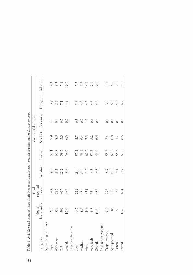
154
Tab
le11.9
.2.
Rep
orte
dca
use
sof
shee
pde
ath
byagr
o-ec
olog
icalzo
nes
,live
stoc
kde
nsi
ties
and
prod
uct
ion
syst
ems.
Cat
ego
ries
No
.o
fh
ou
seh
old
s
To
tal
rep
ort
edca
ses
Cau
ses
of
dea
th(%
)
Pre
dat
ors
Dis
ease
Acc
iden
tP
ois
on
ing
Dro
ugh
tU
nkn
ow
n
Agr
o-e
colo
gica
lzo
nes
Deg
a220
328
19.5
53.4
7.9
1.2
3.7
14.3
Wei
nadeg
a523
722
18.1
61.5
8.0
0.4
2.6
9.3
Kol
la308
437
22.7
59.0
3.0
0.5
7.1
7.8
Ove
rall
1051
1487
19.8
59.0
6.5
0.6
4.2
10.0
Liv
esto
ckd
ensi
ties
Lo
w147
222
28.4
57.2
2.7
0.5
3.6
7.7
Med
ium
323
481
25.6
58.2
6.4
0.2
4.0
5.6
Hig
h346
453
13.2
60.0
7.3
1.1
4.2
14.1
Ver
yh
igh
235
331
14.5
59.8
8.2
0.6
4.8
12.1
Ove
rall
1051
1487
19.8
59.0
6.5
0.6
4.2
10.0
Pro
du
ctio
nsy
stem
s
Cro
p–li
vest
ock
910
1277
18.7
58.7
7.4
0.6
3.4
11.1
Agr
o-p
asto
ral
88
121
24.0
63.6
0.8
0.8
5.8
5.0
Pas
tora
l51
86
29.1
55.8
1.2
0.0
14.0
0.0
Ove
rall
1049
1484
19.7
59.0
6.5
0.6
4.2
10.0
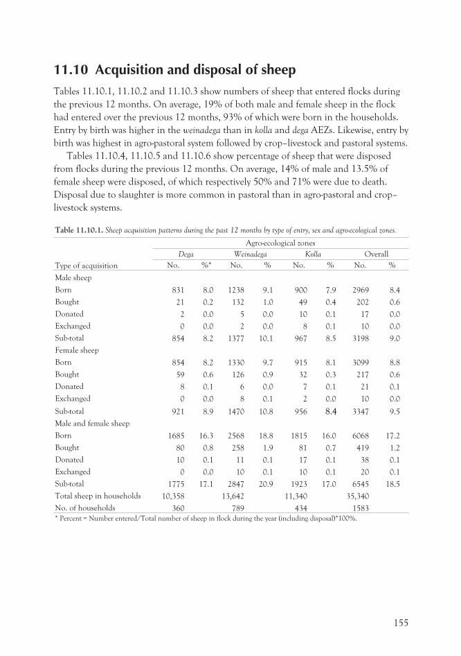
11.10 Acquisition and disposal of sheepTables 11.10.1, 11.10.2 and 11.10.3 show numbers of sheep that entered flocks during
the previous 12 months. On average, 19% of both male and female sheep in the flock
had entered over the previous 12 months, 93% of which were born in the households.
Entry by birth was higher in the weinadega than in kolla and dega AEZs. Likewise, entry by
birth was highest in agro-pastoral system followed by crop–livestock and pastoral systems.
Tables 11.10.4, 11.10.5 and 11.10.6 show percentage of sheep that were disposed
from flocks during the previous 12 months. On average, 14% of male and 13.5% of
female sheep were disposed, of which respectively 50% and 71% were due to death.
Disposal due to slaughter is more common in pastoral than in agro-pastoral and crop–
livestock systems.
Table 11.10.1. Sheep acquisition patterns during the past 12 months by type of entry, sex and agro-ecological zones.
Type of acquisition
Agro-ecological zones
Dega Weinadega Kolla Overall
No. %* No. % No. % No. %
Male sheep
Born 831 8.0 1238 9.1 900 7.9 2969 8.4
Bought 21 0.2 132 1.0 49 0.4 202 0.6
Donated 2 0.0 5 0.0 10 0.1 17 0.0
Exchanged 0 0.0 2 0.0 8 0.1 10 0.0
Sub-total 854 8.2 1377 10.1 967 8.5 3198 9.0
Female sheep
Born 854 8.2 1330 9.7 915 8.1 3099 8.8
Bought 59 0.6 126 0.9 32 0.3 217 0.6
Donated 8 0.1 6 0.0 7 0.1 21 0.1
Exchanged 0 0.0 8 0.1 2 0.0 10 0.0
Sub-total 921 8.9 1470 10.8 956 8.4 3347 9.5
Male and female sheep
Born 1685 16.3 2568 18.8 1815 16.0 6068 17.2
Bought 80 0.8 258 1.9 81 0.7 419 1.2
Donated 10 0.1 11 0.1 17 0.1 38 0.1
Exchanged 0 0.0 10 0.1 10 0.1 20 0.1
Sub-total 1775 17.1 2847 20.9 1923 17.0 6545 18.5
Total sheep in households 10,358 13,642 11,340 35,340
No. of households 360 789 434 1583
* Percent = Number entered/Total number of sheep in flock during the year (including disposal)*100%.
155
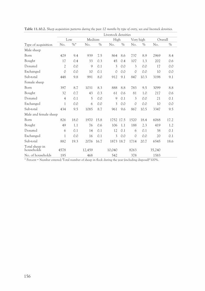
Table 11.10.2. Sheep acquisition patterns during the past 12 months by type of entry, sex and livestock densities.
Type of acquisition
Livestock densities
Low Medium High Very high Overall
No. %* No. % No. % No. % No. %
Male sheep
Born 429 9.4 939 7.5 864 8.6 737 8.9 2969 8.4
Bought 17 0.4 33 0.3 45 0.4 107 1.3 202 0.6
Donated 2 0.0 9 0.1 3 0.0 3 0.0 17 0.0
Exchanged 0 0.0 10 0.1 0 0.0 0 0.0 10 0.0
Sub-total 448 9.8 991 8.0 912 9.1 847 10.3 3198 9.1
Female sheep
Born 397 8.7 1031 8.3 888 8.8 783 9.5 3099 8.8
Bought 32 0.7 43 0.3 61 0.6 81 1.0 217 0.6
Donated 4 0.1 5 0.0 9 0.1 3 0.0 21 0.1
Exchanged 1 0.0 6 0.0 3 0.0 0 0.0 10 0.0
Sub-total 434 9.5 1085 8.7 961 9.6 867 10.5 3347 9.5
Male and female sheep
Born 826 18.0 1970 15.8 1752 17.5 1520 18.4 6068 17.2
Bought 49 1.1 76 0.6 106 1.1 188 2.3 419 1.2
Donated 6 0.1 14 0.1 12 0.1 6 0.1 38 0.1
Exchanged 1 0.0 16 0.1 3 0.0 0 0.0 20 0.1
Sub-total 882 19.3 2076 16.7 1873 18.7 1714 20.7 6545 18.6
Total sheep inhouseholds 4578 12,459 10,040 8263 35,240
No. of households 195 468 542 378 1583
* Percent = Number entered/Total number of sheep in flock during the year (including disposal)*100%.
156
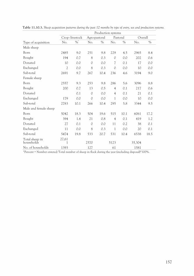
157
Table 11.10.3. Sheep acquisition patterns during the past 12 months by type of entry, sex and production systems.
Type of acquisition
Production systems
Crop–livestock Agro-pastoral Pastoral Overall
No. %* No. % No. % No. %
Male sheep
Born 2485 9.0 251 9.8 229 4.5 2965 8.4
Bought 194 0.7 8 0.3 0 0.0 202 0.6
Donated 10 0.0 0 0.0 7 0.1 17 0.0
Exchanged 2 0.0 8 0.3 0 0.0 10 0.0
Sub-total 2691 9.7 267 10.4 236 4.6 3194 9.0
Female sheep
Born 2557 9.3 253 9.8 286 5.6 3096 8.8
Bought 200 0.7 13 0.5 4 0.1 217 0.6
Donated 0.1 0 0.0 4 0.1 21 0.1
Exchanged 179 0.0 0 0.0 1 0.0 10 0.0
Sub-total 2783 10.1 266 10.4 295 5.8 3344 9.5
Male and female sheep
Born 5042 18.3 504 19.6 515 10.1 6061 17.2
Bought 394 1.4 21 0.8 4 0.1 419 1.2
Donated 27 0.1 0 0.0 11 0.2 38 0.1
Exchanged 11 0.0 8 0.3 1 0.0 20 0.1
Sub-total 5474 19.8 533 20.7 531 10.4 6538 18.5
Total sheep inhouseholds
27,611 2570 5123 35,304
No. of households 1393 127 61 1581
*Percent = Number entered/Total number of sheep in flock during the year (including disposal)*100%.
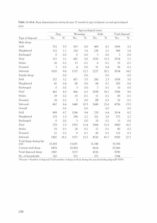
Table 11.10.4. Sheep disposal patterns during the past 12 months by type of disposal, sex and agro-ecological
zones.
Type of disposal
Agro-ecological zones
Dega Weinadega Kolla Total disposal
No. %* No. % No. % No. %
Male sheep
Sold 572 5.5 815 6.0 469 4.1 1856 5.2
Slaughtered 112 1.1 218 1.6 238 2.1 568 1.6
Exchanged 0 0.0 0 0.0 3 0.0 3 0.0
Died 317 3.1 687 5.0 1510 13.3 2514 7.1
Stolen 16 0.2 13 0.1 6 0.1 35 0.1
Donated 3 0.0 4 0.0 51 0.4 58 0.2
Sub-total 1020 9.8 1737 12.7 2277 20.1 5034 14.2
Female sheep 0.0 0.0 0.0 0.0
Sold 327 3.2 471 3.5 260 2.3 1058 3.0
Slaughtered 41 0.4 80 0.6 84 0.7 205 0.6
Exchanged 0 0.0 3 0.0 7 0.1 10 0.0
Died 462 4.5 866 6.3 2058 18.1 3386 9.6
Stolen 19 0.2 15 0.1 11 0.1 45 0.1
Donated 18 0.2 5 0.0 29 0.3 52 0.1
Sub-total 867 8.4 1440 10.5 2449 21.6 4756 13.5
Overall 0.0 0.0 0.0 0.0
Sold 899 8.7 1286 9.4 729 6.4 2914 8.2
Slaughtered 153 1.5 298 2.2 322 2.8 773 2.2
Exchanged 0 0.0 3 0.0 10 0.1 13 0.0
Died 779 7.5 1553 11.4 3568 31.5 5900 16.7
Stolen 35 0.3 28 0.2 17 0.1 80 0.2
Donated 21 0.2 9 0.1 80 0.7 110 0.3
Sub-total 1887 18.2 3177 23.3 4726 41.7 9790 27.7
Total sheep during theyear 10,365 13,651 11,340 35,356
Current total sheep 8478 10,474 6614 25,566
Total disposed sheep 1887 3177 4726 9790
No. of households 320 703 371 1394
*Percent = Number of disposal/Total number of sheep in flock during the year (including disposal)*100%.
158
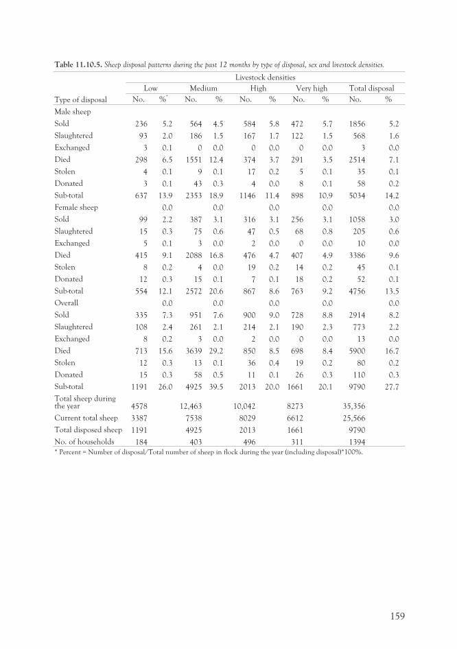
Table 11.10.5. Sheep disposal patterns during the past 12 months by type of disposal, sex and livestock densities.
Type of disposal
Livestock densities
Low Medium High Very high Total disposal
No. %* No. % No. % No. % No. %
Male sheep
Sold 236 5.2 564 4.5 584 5.8 472 5.7 1856 5.2
Slaughtered 93 2.0 186 1.5 167 1.7 122 1.5 568 1.6
Exchanged 3 0.1 0 0.0 0 0.0 0 0.0 3 0.0
Died 298 6.5 1551 12.4 374 3.7 291 3.5 2514 7.1
Stolen 4 0.1 9 0.1 17 0.2 5 0.1 35 0.1
Donated 3 0.1 43 0.3 4 0.0 8 0.1 58 0.2
Sub-total 637 13.9 2353 18.9 1146 11.4 898 10.9 5034 14.2
Female sheep 0.0 0.0 0.0 0.0 0.0
Sold 99 2.2 387 3.1 316 3.1 256 3.1 1058 3.0
Slaughtered 15 0.3 75 0.6 47 0.5 68 0.8 205 0.6
Exchanged 5 0.1 3 0.0 2 0.0 0 0.0 10 0.0
Died 415 9.1 2088 16.8 476 4.7 407 4.9 3386 9.6
Stolen 8 0.2 4 0.0 19 0.2 14 0.2 45 0.1
Donated 12 0.3 15 0.1 7 0.1 18 0.2 52 0.1
Sub-total 554 12.1 2572 20.6 867 8.6 763 9.2 4756 13.5
Overall 0.0 0.0 0.0 0.0 0.0
Sold 335 7.3 951 7.6 900 9.0 728 8.8 2914 8.2
Slaughtered 108 2.4 261 2.1 214 2.1 190 2.3 773 2.2
Exchanged 8 0.2 3 0.0 2 0.0 0 0.0 13 0.0
Died 713 15.6 3639 29.2 850 8.5 698 8.4 5900 16.7
Stolen 12 0.3 13 0.1 36 0.4 19 0.2 80 0.2
Donated 15 0.3 58 0.5 11 0.1 26 0.3 110 0.3
Sub-total 1191 26.0 4925 39.5 2013 20.0 1661 20.1 9790 27.7
Total sheep duringthe year 4578 12,463 10,042 8273 35,356
Current total sheep 3387 7538 8029 6612 25,566
Total disposed sheep 1191 4925 2013 1661 9790
No. of households 184 403 496 311 1394
* Percent = Number of disposal/Total number of sheep in flock during the year (including disposal)*100%.
159
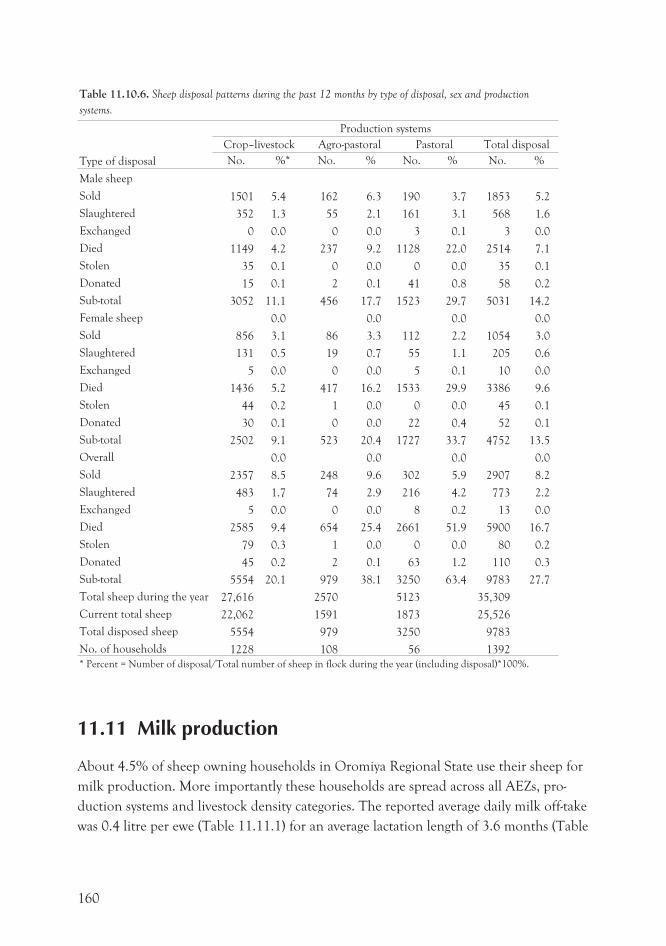
Table 11.10.6. Sheep disposal patterns during the past 12 months by type of disposal, sex and production
systems.
Type of disposal
Production systems
Crop–livestock Agro-pastoral Pastoral Total disposal
No. %* No. % No. % No. %
Male sheep
Sold 1501 5.4 162 6.3 190 3.7 1853 5.2
Slaughtered 352 1.3 55 2.1 161 3.1 568 1.6
Exchanged 0 0.0 0 0.0 3 0.1 3 0.0
Died 1149 4.2 237 9.2 1128 22.0 2514 7.1
Stolen 35 0.1 0 0.0 0 0.0 35 0.1
Donated 15 0.1 2 0.1 41 0.8 58 0.2
Sub-total 3052 11.1 456 17.7 1523 29.7 5031 14.2
Female sheep 0.0 0.0 0.0 0.0
Sold 856 3.1 86 3.3 112 2.2 1054 3.0
Slaughtered 131 0.5 19 0.7 55 1.1 205 0.6
Exchanged 5 0.0 0 0.0 5 0.1 10 0.0
Died 1436 5.2 417 16.2 1533 29.9 3386 9.6
Stolen 44 0.2 1 0.0 0 0.0 45 0.1
Donated 30 0.1 0 0.0 22 0.4 52 0.1
Sub-total 2502 9.1 523 20.4 1727 33.7 4752 13.5
Overall 0.0 0.0 0.0 0.0
Sold 2357 8.5 248 9.6 302 5.9 2907 8.2
Slaughtered 483 1.7 74 2.9 216 4.2 773 2.2
Exchanged 5 0.0 0 0.0 8 0.2 13 0.0
Died 2585 9.4 654 25.4 2661 51.9 5900 16.7
Stolen 79 0.3 1 0.0 0 0.0 80 0.2
Donated 45 0.2 2 0.1 63 1.2 110 0.3
Sub-total 5554 20.1 979 38.1 3250 63.4 9783 27.7
Total sheep during the year 27,616 2570 5123 35,309
Current total sheep 22,062 1591 1873 25,526
Total disposed sheep 5554 979 3250 9783
No. of households 1228 108 56 1392
* Percent = Number of disposal/Total number of sheep in flock during the year (including disposal)*100%.
11.11 Milk production
About 4.5% of sheep owning households in Oromiya Regional State use their sheep for
milk production. More importantly these households are spread across all AEZs, pro-
duction systems and livestock density categories. The reported average daily milk off-take
was 0.4 litre per ewe (Table 11.11.1) for an average lactation length of 3.6 months (Table
160
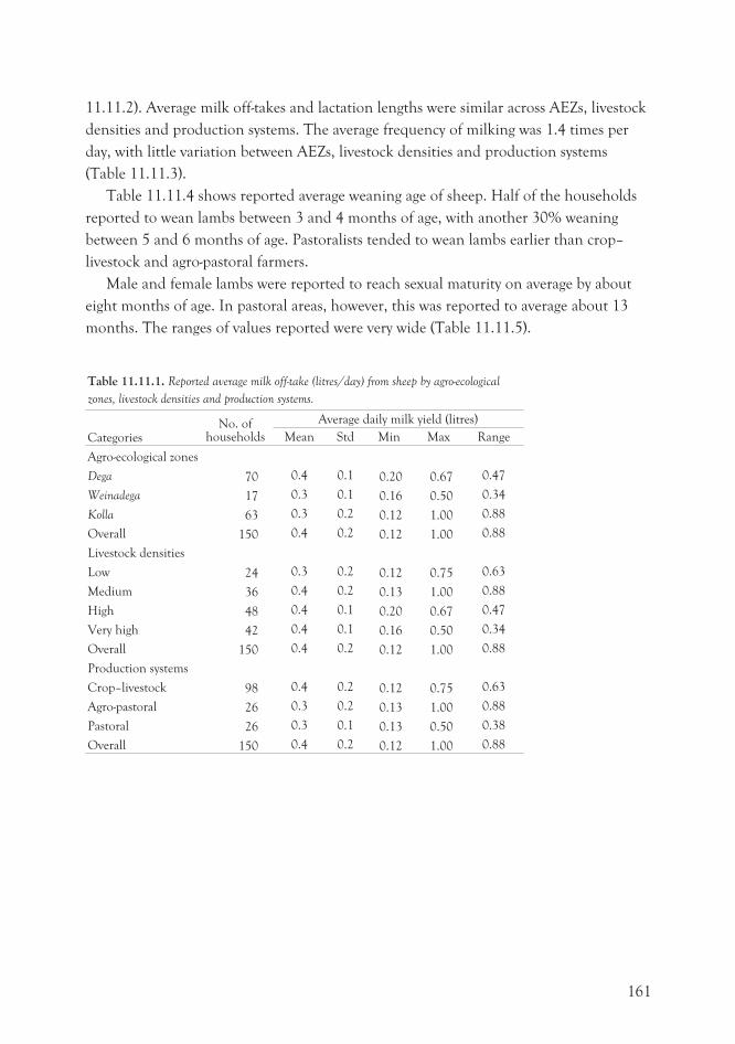
11.11.2). Average milk off-takes and lactation lengths were similar across AEZs, livestock
densities and production systems. The average frequency of milking was 1.4 times per
day, with little variation between AEZs, livestock densities and production systems
(Table 11.11.3).
Table 11.11.4 shows reported average weaning age of sheep. Half of the households
reported to wean lambs between 3 and 4 months of age, with another 30% weaning
between 5 and 6 months of age. Pastoralists tended to wean lambs earlier than crop–
livestock and agro-pastoral farmers.
Male and female lambs were reported to reach sexual maturity on average by about
eight months of age. In pastoral areas, however, this was reported to average about 13
months. The ranges of values reported were very wide (Table 11.11.5).
Table 11.11.1. Reported average milk off-take (litres/day) from sheep by agro-ecological
zones, livestock densities and production systems.
CategoriesNo. of
households
Average daily milk yield (litres)
Mean Std Min Max Range
Agro-ecological zones
Dega 70 0.4 0.1 0.20 0.67 0.47
Weinadega 17 0.3 0.1 0.16 0.50 0.34
Kolla 63 0.3 0.2 0.12 1.00 0.88
Overall 150 0.4 0.2 0.12 1.00 0.88
Livestock densities
Low 24 0.3 0.2 0.12 0.75 0.63
Medium 36 0.4 0.2 0.13 1.00 0.88
High 48 0.4 0.1 0.20 0.67 0.47
Very high 42 0.4 0.1 0.16 0.50 0.34
Overall 150 0.4 0.2 0.12 1.00 0.88
Production systems
Crop–livestock 98 0.4 0.2 0.12 0.75 0.63
Agro-pastoral 26 0.3 0.2 0.13 1.00 0.88
Pastoral 26 0.3 0.1 0.13 0.50 0.38
Overall 150 0.4 0.2 0.12 1.00 0.88
161
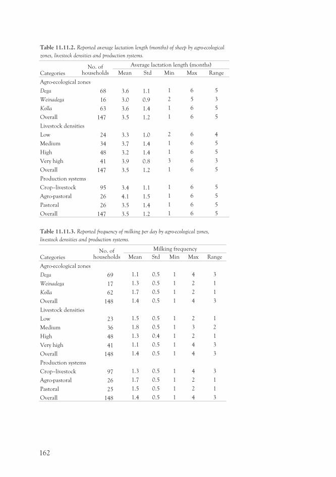
Table 11.11.2. Reported average lactation length (months) of sheep by agro-ecological
zones, livestock densities and production systems.
CategoriesNo. of
households
Average lactation length (months)
Mean Std Min Max Range
Agro-ecological zones
Dega 68 3.6 1.1 1 6 5
Weinadega 16 3.0 0.9 2 5 3
Kolla 63 3.6 1.4 1 6 5
Overall 147 3.5 1.2 1 6 5
Livestock densities
Low 24 3.3 1.0 2 6 4
Medium 34 3.7 1.4 1 6 5
High 48 3.2 1.4 1 6 5
Very high 41 3.9 0.8 3 6 3
Overall 147 3.5 1.2 1 6 5
Production systems
Crop–livestock 95 3.4 1.1 1 6 5
Agro-pastoral 26 4.1 1.5 1 6 5
Pastoral 26 3.5 1.4 1 6 5
Overall 147 3.5 1.2 1 6 5
Table 11.11.3. Reported frequency of milking per day by agro-ecological zones,
livestock densities and production systems.
CategoriesNo. of
households
Milking frequency
Mean Std Min Max Range
Agro-ecological zones
Dega 69 1.1 0.5 1 4 3
Weinadega 17 1.3 0.5 1 2 1
Kolla 62 1.7 0.5 1 2 1
Overall 148 1.4 0.5 1 4 3
Livestock densities
Low 23 1.5 0.5 1 2 1
Medium 36 1.8 0.5 1 3 2
High 48 1.3 0.4 1 2 1
Very high 41 1.1 0.5 1 4 3
Overall 148 1.4 0.5 1 4 3
Production systems
Crop–livestock 97 1.3 0.5 1 4 3
Agro-pastoral 26 1.7 0.5 1 2 1
Pastoral 25 1.5 0.5 1 2 1
Overall 148 1.4 0.5 1 4 3
162
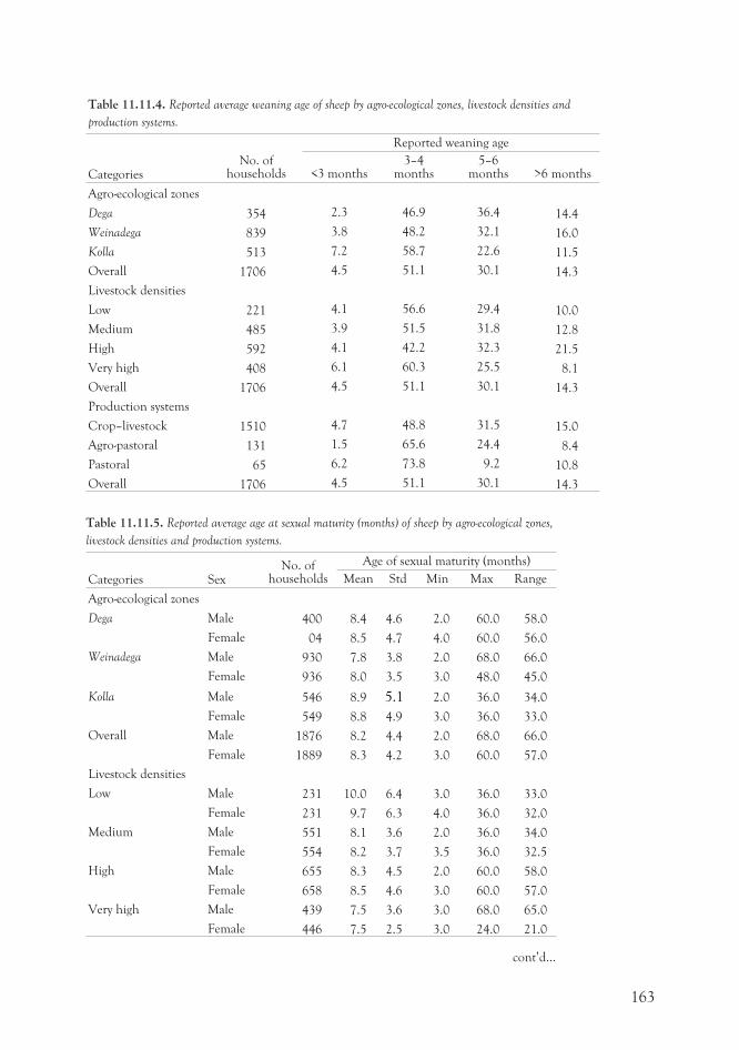
Table 11.11.4. Reported average weaning age of sheep by agro-ecological zones, livestock densities and
production systems.
CategoriesNo. of
households
Reported weaning age
<3 months3–4
months5–6
months >6 months
Agro-ecological zones
Dega 354 2.3 46.9 36.4 14.4
Weinadega 839 3.8 48.2 32.1 16.0
Kolla 513 7.2 58.7 22.6 11.5
Overall 1706 4.5 51.1 30.1 14.3
Livestock densities
Low 221 4.1 56.6 29.4 10.0
Medium 485 3.9 51.5 31.8 12.8
High 592 4.1 42.2 32.3 21.5
Very high 408 6.1 60.3 25.5 8.1
Overall 1706 4.5 51.1 30.1 14.3
Production systems
Crop–livestock 1510 4.7 48.8 31.5 15.0
Agro-pastoral 131 1.5 65.6 24.4 8.4
Pastoral 65 6.2 73.8 9.2 10.8
Overall 1706 4.5 51.1 30.1 14.3
Table 11.11.5. Reported average age at sexual maturity (months) of sheep by agro-ecological zones,
livestock densities and production systems.
Categories SexNo. of
households
Age of sexual maturity (months)
Mean Std Min Max Range
Agro-ecological zones
Dega Male 400 8.4 4.6 2.0 60.0 58.0
Female 04 8.5 4.7 4.0 60.0 56.0
Weinadega Male 930 7.8 3.8 2.0 68.0 66.0
Female 936 8.0 3.5 3.0 48.0 45.0
Kolla Male 546 8.9 5.1 2.0 36.0 34.0
Female 549 8.8 4.9 3.0 36.0 33.0
Overall Male 1876 8.2 4.4 2.0 68.0 66.0
Female 1889 8.3 4.2 3.0 60.0 57.0
Livestock densities
Low Male 231 10.0 6.4 3.0 36.0 33.0
Female 231 9.7 6.3 4.0 36.0 32.0
Medium Male 551 8.1 3.6 2.0 36.0 34.0
Female 554 8.2 3.7 3.5 36.0 32.5
High Male 655 8.3 4.5 2.0 60.0 58.0
Female 658 8.5 4.6 3.0 60.0 57.0
Very high Male 439 7.5 3.6 3.0 68.0 65.0
Female 446 7.5 2.5 3.0 24.0 21.0
163
cont’d...
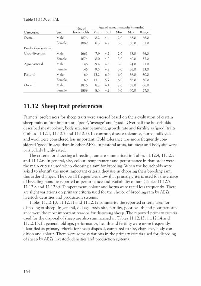
Categories SexNo. of
households
Age of sexual maturity (months)
Mean Std Min Max Range
Overall Male 1876 8.2 4.4 2.0 68.0 66.0
Female 1889 8.3 4.2 3.0 60.0 57.0
Production systems
Crop–livestock Male 1661 7.9 4.2 2.0 68.0 66.0
Female 1674 8.0 4.0 3.0 60.0 57.0
Agro-pastoral Male 146 9.4 4.5 3.0 24.0 21.0
Female 146 9.5 4.8 3.0 36.0 33.0
Pastoral Male 69 13.2 6.0 6.0 36.0 30.0
Female 69 13.1 5.7 6.0 36.0 30.0
Overall Male 1876 8.2 4.4 2.0 68.0 66.0
Female 1889 8.3 4.2 3.0 60.0 57.0
11.12 Sheep trait preferences
Farmers’ preferences for sheep traits were assessed based on their evaluation of certain
sheep traits as ‘not important’, ‘poor’, ‘average’ and ‘good’. Over half the households
described meat, colour, body size, temperament, growth rate and fertility as ‘good’ traits
(Tables 11.12.1, 11.12.2 and 11.12.3). In contrast, disease tolerance, horns, milk yield
and wool were considered less important. Cold tolerance was more frequently con-
sidered ‘good’ in dega than in other AEZs. In pastoral areas, fat, meat and body size were
particularly highly rated.
The criteria for choosing a breeding ram are summarised in Tables 11.12.4, 11.12.5
and 11.12.6. In general, size, colour, temperament and performance in that order were
the main criteria used when choosing a ram for breeding. When the households were
asked to identify the most important criteria they use in choosing their breeding ram,
this order changes. The overall frequencies show that primary criteria used for the choice
of breeding rams are reported as performance and availability of ram (Tables 11.12.7,
11.12.8 and 11.12.9). Temperament, colour and horns were rated less frequently. There
are slight variations on primary criteria used for the choice of breeding ram by AEZs,
livestock densities and production systems.
Tables 11.12.10, 11.12.11 and 11.12.12 summarise the reported criteria used for
disposing of sheep. In general, old age, body size, fertility, poor health and poor perform-
ance were the most important reasons for disposing sheep. The reported primary criteria
used for the disposal of sheep are also summarised in Tables 11.12.13, 11.12.14 and
11.12.15. In general, old age, performance, health and fertility were more frequently
identified as primary criteria for sheep disposal, compared to size, character, body con-
dition and colour. There were some variations in the primary criteria used for disposing
of sheep by AEZs, livestock densities and production systems.
164
Table 11.11.5. cont’d.
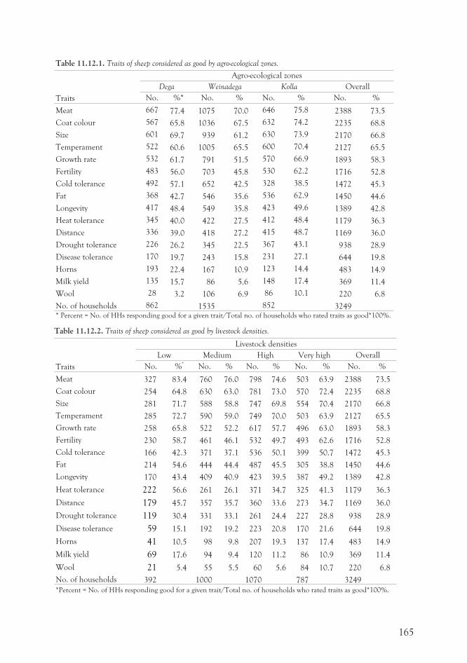
Table 11.12.1. Traits of sheep considered as good by agro-ecological zones.
Traits
Agro-ecological zones
Dega Weinadega Kolla Overall
No. %* No. % No. % No. %
Meat 667 77.4 1075 70.0 646 75.8 2388 73.5
Coat colour 567 65.8 1036 67.5 632 74.2 2235 68.8
Size 601 69.7 939 61.2 630 73.9 2170 66.8
Temperament 522 60.6 1005 65.5 600 70.4 2127 65.5
Growth rate 532 61.7 791 51.5 570 66.9 1893 58.3
Fertility 483 56.0 703 45.8 530 62.2 1716 52.8
Cold tolerance 492 57.1 652 42.5 328 38.5 1472 45.3
Fat 368 42.7 546 35.6 536 62.9 1450 44.6
Longevity 417 48.4 549 35.8 423 49.6 1389 42.8
Heat tolerance 345 40.0 422 27.5 412 48.4 1179 36.3
Distance 336 39.0 418 27.2 415 48.7 1169 36.0
Drought tolerance 226 26.2 345 22.5 367 43.1 938 28.9
Disease tolerance 170 19.7 243 15.8 231 27.1 644 19.8
Horns 193 22.4 167 10.9 123 14.4 483 14.9
Milk yield 135 15.7 86 5.6 148 17.4 369 11.4
Wool 28 3.2 106 6.9 86 10.1 220 6.8
No. of households 862 1535 852 3249* Percent = No. of HHs responding good for a given trait/Total no. of households who rated traits as good*100%.
Table 11.12.2. Traits of sheep considered as good by livestock densities.
Traits
Livestock densities
Low Medium High Very high Overall
No. %* No. % No. % No. % No. %
Meat 327 83.4 760 76.0 798 74.6 503 63.9 2388 73.5
Coat colour 254 64.8 630 63.0 781 73.0 570 72.4 2235 68.8
Size 281 71.7 588 58.8 747 69.8 554 70.4 2170 66.8
Temperament 285 72.7 590 59.0 749 70.0 503 63.9 2127 65.5
Growth rate 258 65.8 522 52.2 617 57.7 496 63.0 1893 58.3
Fertility 230 58.7 461 46.1 532 49.7 493 62.6 1716 52.8
Cold tolerance 166 42.3 371 37.1 536 50.1 399 50.7 1472 45.3
Fat 214 54.6 444 44.4 487 45.5 305 38.8 1450 44.6
Longevity 170 43.4 409 40.9 423 39.5 387 49.2 1389 42.8
Heat tolerance 222 56.6 261 26.1 371 34.7 325 41.3 1179 36.3
Distance 179 45.7 357 35.7 360 33.6 273 34.7 1169 36.0
Drought tolerance 119 30.4 331 33.1 261 24.4 227 28.8 938 28.9
Disease tolerance 59 15.1 192 19.2 223 20.8 170 21.6 644 19.8
Horns 41 10.5 98 9.8 207 19.3 137 17.4 483 14.9
Milk yield 69 17.6 94 9.4 120 11.2 86 10.9 369 11.4
Wool 21 5.4 55 5.5 60 5.6 84 10.7 220 6.8
No. of households 392 1000 1070 787 3249
*Percent = No. of HHs responding good for a given trait/Total no. of households who rated traits as good*100%.
165
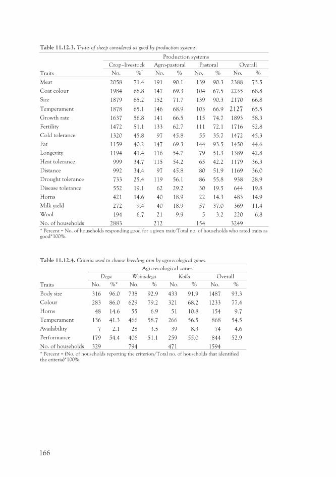
Table 11.12.3. Traits of sheep considered as good by production systems.
Traits
Production systems
Crop–livestock Agro-pastoral Pastoral Overall
No. %* No. % No. % No. %
Meat 2058 71.4 191 90.1 139 90.3 2388 73.5
Coat colour 1984 68.8 147 69.3 104 67.5 2235 68.8
Size 1879 65.2 152 71.7 139 90.3 2170 66.8
Temperament 1878 65.1 146 68.9 103 66.9 2127 65.5
Growth rate 1637 56.8 141 66.5 115 74.7 1893 58.3
Fertility 1472 51.1 133 62.7 111 72.1 1716 52.8
Cold tolerance 1320 45.8 97 45.8 55 35.7 1472 45.3
Fat 1159 40.2 147 69.3 144 93.5 1450 44.6
Longevity 1194 41.4 116 54.7 79 51.3 1389 42.8
Heat tolerance 999 34.7 115 54.2 65 42.2 1179 36.3
Distance 992 34.4 97 45.8 80 51.9 1169 36.0
Drought tolerance 733 25.4 119 56.1 86 55.8 938 28.9
Disease tolerance 552 19.1 62 29.2 30 19.5 644 19.8
Horns 421 14.6 40 18.9 22 14.3 483 14.9
Milk yield 272 9.4 40 18.9 57 37.0 369 11.4
Wool 194 6.7 21 9.9 5 3.2 220 6.8
No. of households 2883 212 154 3249
* Percent = No. of households responding good for a given trait/Total no. of households who rated traits asgood*100%.
Table 11.12.4. Criteria used to choose breeding ram by agro-ecological zones.
Traits
Agro-ecological zones
Dega Weinadega Kolla Overall
No. %* No. % No. % No. %
Body size 316 96.0 738 92.9 433 91.9 1487 93.3
Colour 283 86.0 629 79.2 321 68.2 1233 77.4
Horns 48 14.6 55 6.9 51 10.8 154 9.7
Temperament 136 41.3 466 58.7 266 56.5 868 54.5
Availability 7 2.1 28 3.5 39 8.3 74 4.6
Performance 179 54.4 406 51.1 259 55.0 844 52.9
No. of households 329 794 471 1594
* Percent = (No. of households reporting the criterion/Total no. of households that identifiedthe criteria)*100%.
166
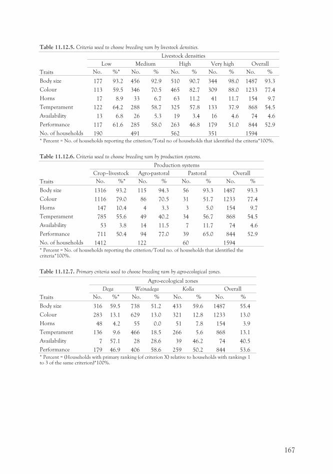
Table 11.12.5. Criteria used to choose breeding ram by livestock densities.
Traits
Livestock densities
Low Medium High Very high Overall
No. %* No. % No. % No. % No. %
Body size 177 93.2 456 92.9 510 90.7 344 98.0 1487 93.3
Colour 113 59.5 346 70.5 465 82.7 309 88.0 1233 77.4
Horns 17 8.9 33 6.7 63 11.2 41 11.7 154 9.7
Temperament 122 64.2 288 58.7 325 57.8 133 37.9 868 54.5
Availability 13 6.8 26 5.3 19 3.4 16 4.6 74 4.6
Performance 117 61.6 285 58.0 263 46.8 179 51.0 844 52.9
No. of households 190 491 562 351 1594
* Percent = No. of households reporting the criterion/Total no of households that identified the criteria*100%.
Table 11.12.6. Criteria used to choose breeding ram by production systems.
Traits
Production systems
Crop–livestock Agro-pastoral Pastoral Overall
No. %* No. % No. % No. %
Body size 1316 93.2 115 94.3 56 93.3 1487 93.3
Colour 1116 79.0 86 70.5 31 51.7 1233 77.4
Horns 147 10.4 4 3.3 3 5.0 154 9.7
Temperament 785 55.6 49 40.2 34 56.7 868 54.5
Availability 53 3.8 14 11.5 7 11.7 74 4.6
Performance 711 50.4 94 77.0 39 65.0 844 52.9
No. of households 1412 122 60 1594
* Percent = No. of households reporting the criterion/Total no. of households that identified thecriteria*100%.
Table 11.12.7. Primary criteria used to choose breeding ram by agro-ecological zones.
Traits
Agro-ecological zones
Dega Weinadega Kolla Overall
No. %* No. % No. % No. %
Body size 316 59.5 738 51.2 433 59.6 1487 55.4
Colour 283 13.1 629 13.0 321 12.8 1233 13.0
Horns 48 4.2 55 0.0 51 7.8 154 3.9
Temperament 136 9.6 466 18.5 266 5.6 868 13.1
Availability 7 57.1 28 28.6 39 46.2 74 40.5
Performance 179 46.9 406 58.6 259 50.2 844 53.6
* Percent = (Households with primary ranking (of criterion X) relative to households with rankings 1to 3 of the same criterion)*100%.
167
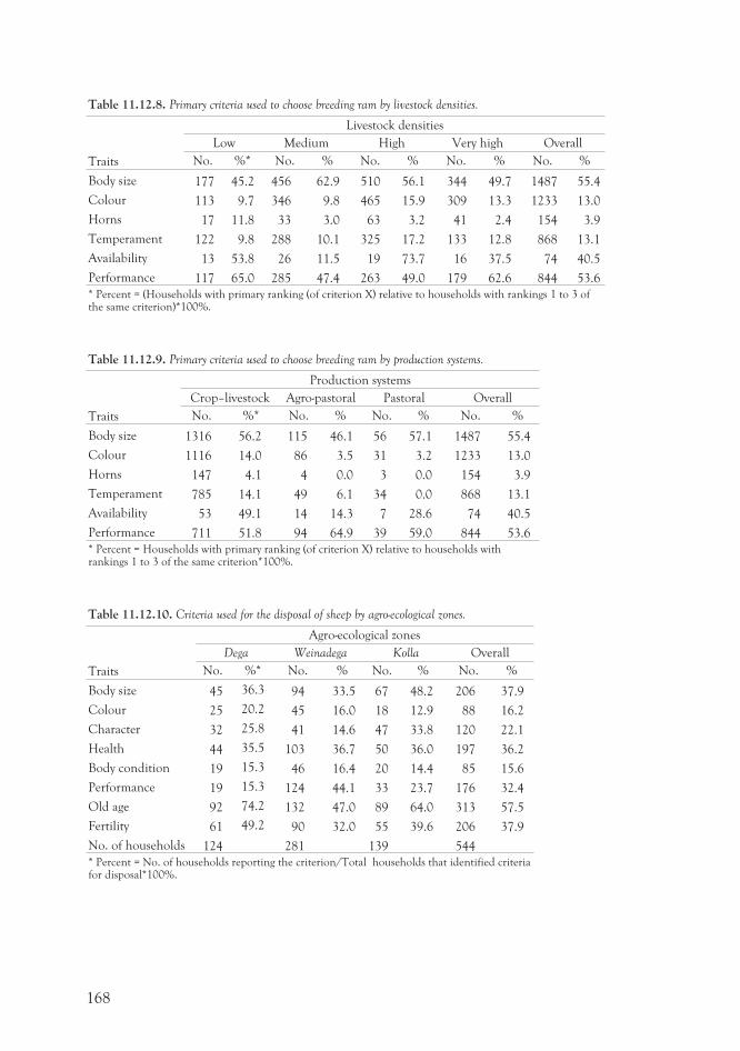
Table 11.12.8. Primary criteria used to choose breeding ram by livestock densities.
Traits
Livestock densities
Low Medium High Very high Overall
No. %* No. % No. % No. % No. %
Body size 177 45.2 456 62.9 510 56.1 344 49.7 1487 55.4
Colour 113 9.7 346 9.8 465 15.9 309 13.3 1233 13.0
Horns 17 11.8 33 3.0 63 3.2 41 2.4 154 3.9
Temperament 122 9.8 288 10.1 325 17.2 133 12.8 868 13.1
Availability 13 53.8 26 11.5 19 73.7 16 37.5 74 40.5
Performance 117 65.0 285 47.4 263 49.0 179 62.6 844 53.6
* Percent = (Households with primary ranking (of criterion X) relative to households with rankings 1 to 3 ofthe same criterion)*100%.
Table 11.12.9. Primary criteria used to choose breeding ram by production systems.
Traits
Production systems
Crop–livestock Agro-pastoral Pastoral Overall
No. %* No. % No. % No. %
Body size 1316 56.2 115 46.1 56 57.1 1487 55.4
Colour 1116 14.0 86 3.5 31 3.2 1233 13.0
Horns 147 4.1 4 0.0 3 0.0 154 3.9
Temperament 785 14.1 49 6.1 34 0.0 868 13.1
Availability 53 49.1 14 14.3 7 28.6 74 40.5
Performance 711 51.8 94 64.9 39 59.0 844 53.6
* Percent = Households with primary ranking (of criterion X) relative to households withrankings 1 to 3 of the same criterion*100%.
Table 11.12.10. Criteria used for the disposal of sheep by agro-ecological zones.
Traits
Agro-ecological zones
Dega Weinadega Kolla Overall
No. %* No. % No. % No. %
Body size 45 36.3 94 33.5 67 48.2 206 37.9
Colour 25 20.2 45 16.0 18 12.9 88 16.2
Character 32 25.8 41 14.6 47 33.8 120 22.1
Health 44 35.5 103 36.7 50 36.0 197 36.2
Body condition 19 15.3 46 16.4 20 14.4 85 15.6
Performance 19 15.3 124 44.1 33 23.7 176 32.4
Old age 92 74.2 132 47.0 89 64.0 313 57.5
Fertility 61 49.2 90 32.0 55 39.6 206 37.9
No. of households 124 281 139 544
* Percent = No. of households reporting the criterion/Total households that identified criteriafor disposal*100%.
168
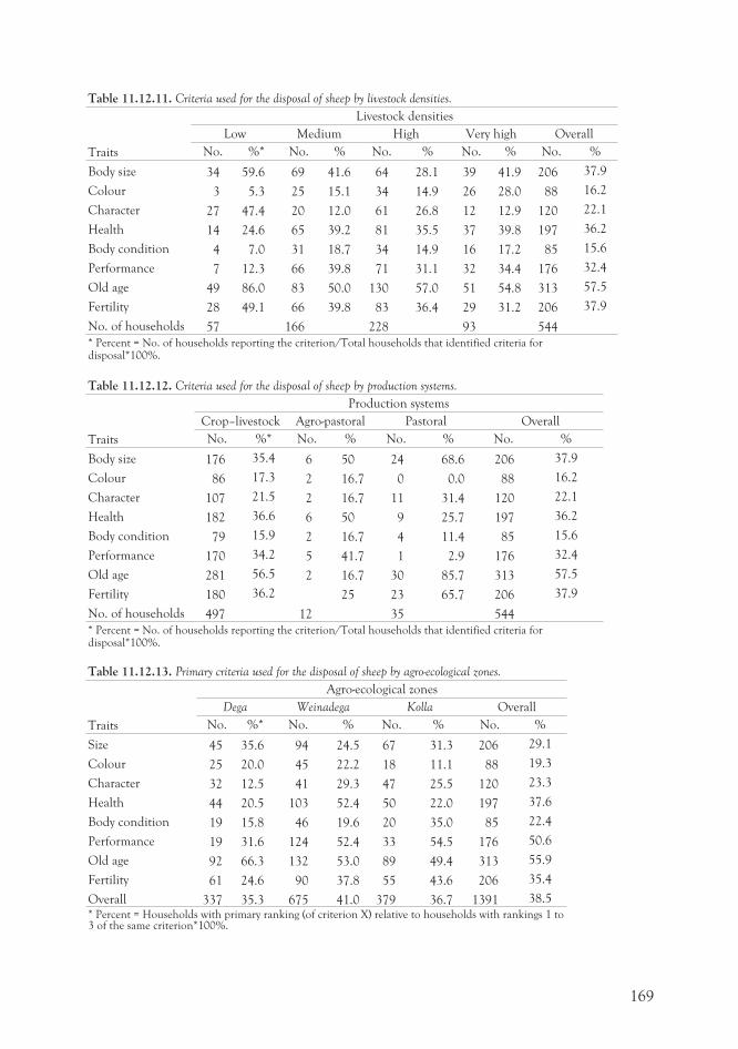
Table 11.12.11. Criteria used for the disposal of sheep by livestock densities.
Traits
Livestock densities
Low Medium High Very high Overall
No. %* No. % No. % No. % No. %
Body size 34 59.6 69 41.6 64 28.1 39 41.9 206 37.9
Colour 3 5.3 25 15.1 34 14.9 26 28.0 88 16.2
Character 27 47.4 20 12.0 61 26.8 12 12.9 120 22.1
Health 14 24.6 65 39.2 81 35.5 37 39.8 197 36.2
Body condition 4 7.0 31 18.7 34 14.9 16 17.2 85 15.6
Performance 7 12.3 66 39.8 71 31.1 32 34.4 176 32.4
Old age 49 86.0 83 50.0 130 57.0 51 54.8 313 57.5
Fertility 28 49.1 66 39.8 83 36.4 29 31.2 206 37.9
No. of households 57 166 228 93 544
* Percent = No. of households reporting the criterion/Total households that identified criteria fordisposal*100%.
Table 11.12.12. Criteria used for the disposal of sheep by production systems.
Traits
Production systems
Crop–livestock Agro-pastoral Pastoral Overall
No. %* No. % No. % No. %
Body size 176 35.4 6 50 24 68.6 206 37.9
Colour 86 17.3 2 16.7 0 0.0 88 16.2
Character 107 21.5 2 16.7 11 31.4 120 22.1
Health 182 36.6 6 50 9 25.7 197 36.2
Body condition 79 15.9 2 16.7 4 11.4 85 15.6
Performance 170 34.2 5 41.7 1 2.9 176 32.4
Old age 281 56.5 2 16.7 30 85.7 313 57.5
Fertility 180 36.2 25 23 65.7 206 37.9
No. of households 497 12 35 544
* Percent = No. of households reporting the criterion/Total households that identified criteria fordisposal*100%.
Table 11.12.13. Primary criteria used for the disposal of sheep by agro-ecological zones.
Traits
Agro-ecological zones
Dega Weinadega Kolla Overall
No. %* No. % No. % No. %
Size 45 35.6 94 24.5 67 31.3 206 29.1
Colour 25 20.0 45 22.2 18 11.1 88 19.3
Character 32 12.5 41 29.3 47 25.5 120 23.3
Health 44 20.5 103 52.4 50 22.0 197 37.6
Body condition 19 15.8 46 19.6 20 35.0 85 22.4
Performance 19 31.6 124 52.4 33 54.5 176 50.6
Old age 92 66.3 132 53.0 89 49.4 313 55.9
Fertility 61 24.6 90 37.8 55 43.6 206 35.4
Overall 337 35.3 675 41.0 379 36.7 1391 38.5
* Percent = Households with primary ranking (of criterion X) relative to households with rankings 1 to3 of the same criterion*100%.
169
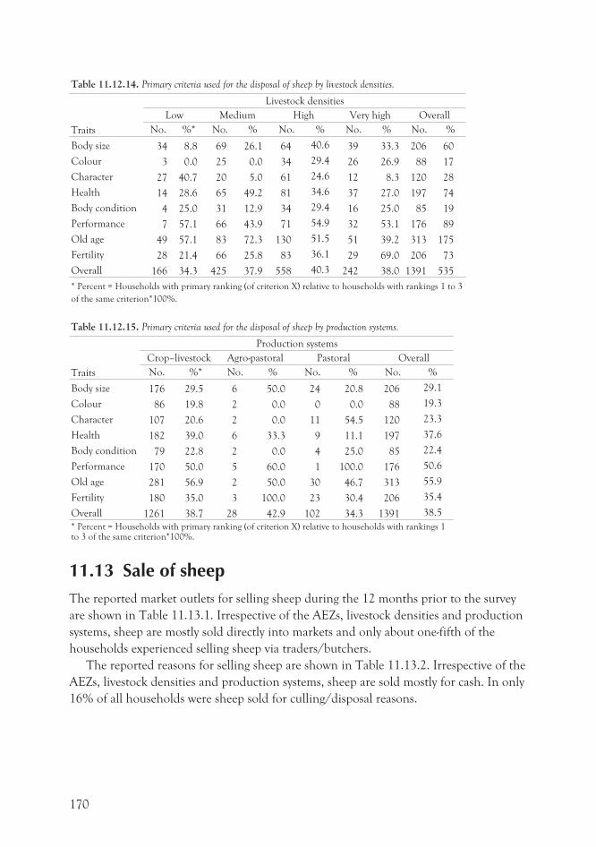
Table 11.12.14. Primary criteria used for the disposal of sheep by livestock densities.
Traits
Livestock densities
Low Medium High Very high Overall
No. %* No. % No. % No. % No. %
Body size 34 8.8 69 26.1 64 40.6 39 33.3 206 60
Colour 3 0.0 25 0.0 34 29.4 26 26.9 88 17
Character 27 40.7 20 5.0 61 24.6 12 8.3 120 28
Health 14 28.6 65 49.2 81 34.6 37 27.0 197 74
Body condition 4 25.0 31 12.9 34 29.4 16 25.0 85 19
Performance 7 57.1 66 43.9 71 54.9 32 53.1 176 89
Old age 49 57.1 83 72.3 130 51.5 51 39.2 313 175
Fertility 28 21.4 66 25.8 83 36.1 29 69.0 206 73
Overall 166 34.3 425 37.9 558 40.3 242 38.0 1391 535
* Percent = Households with primary ranking (of criterion X) relative to households with rankings 1 to 3
of the same criterion*100%.
Table 11.12.15. Primary criteria used for the disposal of sheep by production systems.
Traits
Production systems
Crop–livestock Agro-pastoral Pastoral Overall
No. %* No. % No. % No. %
Body size 176 29.5 6 50.0 24 20.8 206 29.1
Colour 86 19.8 2 0.0 0 0.0 88 19.3
Character 107 20.6 2 0.0 11 54.5 120 23.3
Health 182 39.0 6 33.3 9 11.1 197 37.6
Body condition 79 22.8 2 0.0 4 25.0 85 22.4
Performance 170 50.0 5 60.0 1 100.0 176 50.6
Old age 281 56.9 2 50.0 30 46.7 313 55.9
Fertility 180 35.0 3 100.0 23 30.4 206 35.4
Overall 1261 38.7 28 42.9 102 34.3 1391 38.5
* Percent = Households with primary ranking (of criterion X) relative to households with rankings 1to 3 of the same criterion*100%.
11.13 Sale of sheepThe reported market outlets for selling sheep during the 12 months prior to the survey
are shown in Table 11.13.1. Irrespective of the AEZs, livestock densities and production
systems, sheep are mostly sold directly into markets and only about one-fifth of the
households experienced selling sheep via traders/butchers.
The reported reasons for selling sheep are shown in Table 11.13.2. Irrespective of the
AEZs, livestock densities and production systems, sheep are sold mostly for cash. In only
16% of all households were sheep sold for culling/disposal reasons.
170
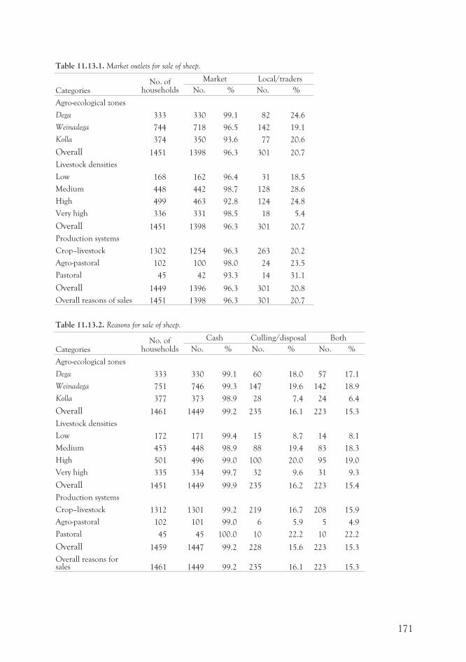
Table 11.13.1. Market outlets for sale of sheep.
CategoriesNo. of
households
Market Local/traders
No. % No. %
Agro-ecological zones
Dega 333 330 99.1 82 24.6
Weinadega 744 718 96.5 142 19.1
Kolla 374 350 93.6 77 20.6
Overall 1451 1398 96.3 301 20.7
Livestock densities
Low 168 162 96.4 31 18.5
Medium 448 442 98.7 128 28.6
High 499 463 92.8 124 24.8
Very high 336 331 98.5 18 5.4
Overall 1451 1398 96.3 301 20.7
Production systems
Crop–livestock 1302 1254 96.3 263 20.2
Agro-pastoral 102 100 98.0 24 23.5
Pastoral 45 42 93.3 14 31.1
Overall 1449 1396 96.3 301 20.8
Overall reasons of sales 1451 1398 96.3 301 20.7
Table 11.13.2. Reasons for sale of sheep.
CategoriesNo. of
households
Cash Culling/disposal Both
No. % No. % No. %
Agro-ecological zones
Dega 333 330 99.1 60 18.0 57 17.1
Weinadega 751 746 99.3 147 19.6 142 18.9
Kolla 377 373 98.9 28 7.4 24 6.4
Overall 1461 1449 99.2 235 16.1 223 15.3
Livestock densities
Low 172 171 99.4 15 8.7 14 8.1
Medium 453 448 98.9 88 19.4 83 18.3
High 501 496 99.0 100 20.0 95 19.0
Very high 335 334 99.7 32 9.6 31 9.3
Overall 1451 1449 99.9 235 16.2 223 15.4
Production systems
Crop–livestock 1312 1301 99.2 219 16.7 208 15.9
Agro-pastoral 102 101 99.0 6 5.9 5 4.9
Pastoral 45 45 100.0 10 22.2 10 22.2
Overall 1459 1447 99.2 228 15.6 223 15.3
Overall reasons forsales 1461 1449 99.2 235 16.1 223 15.3
171
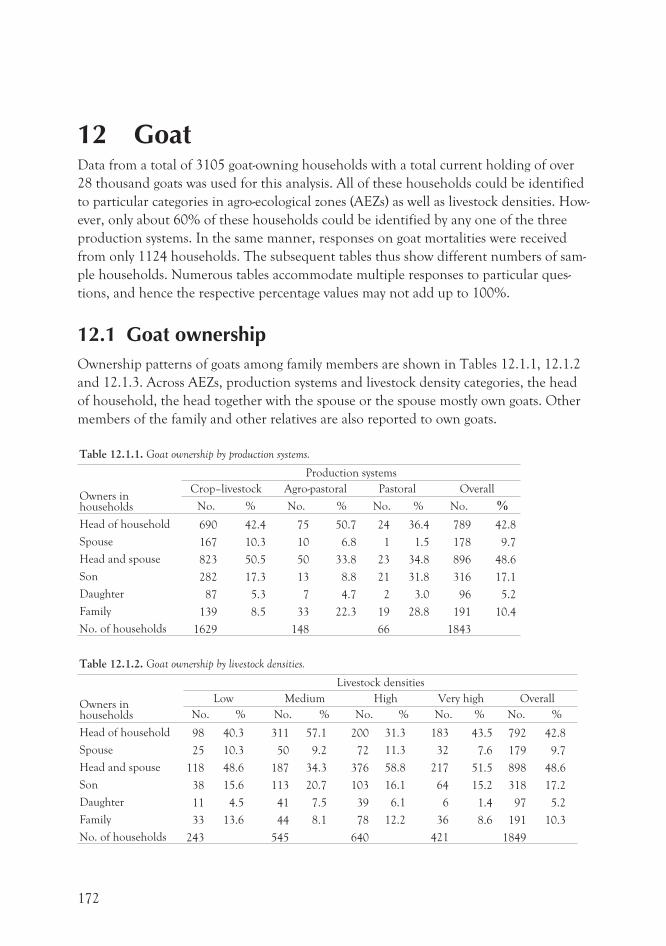
12 GoatData from a total of 3105 goat-owning households with a total current holding of over
28 thousand goats was used for this analysis. All of these households could be identified
to particular categories in agro-ecological zones (AEZs) as well as livestock densities. How-
ever, only about 60% of these households could be identified by any one of the three
production systems. In the same manner, responses on goat mortalities were received
from only 1124 households. The subsequent tables thus show different numbers of sam-
ple households. Numerous tables accommodate multiple responses to particular ques-
tions, and hence the respective percentage values may not add up to 100%.
12.1 Goat ownershipOwnership patterns of goats among family members are shown in Tables 12.1.1, 12.1.2
and 12.1.3. Across AEZs, production systems and livestock density categories, the head
of household, the head together with the spouse or the spouse mostly own goats. Other
members of the family and other relatives are also reported to own goats.
Table 12.1.1. Goat ownership by production systems.
Owners inhouseholds
Production systems
Crop–livestock Agro-pastoral Pastoral Overall
No. % No. % No. % No. %
Head of household 690 42.4 75 50.7 24 36.4 789 42.8
Spouse 167 10.3 10 6.8 1 1.5 178 9.7
Head and spouse 823 50.5 50 33.8 23 34.8 896 48.6
Son 282 17.3 13 8.8 21 31.8 316 17.1
Daughter 87 5.3 7 4.7 2 3.0 96 5.2
Family 139 8.5 33 22.3 19 28.8 191 10.4
No. of households 1629 148 66 1843
Table 12.1.2. Goat ownership by livestock densities.
Owners inhouseholds
Livestock densities
Low Medium High Very high Overall
No. % No. % No. % No. % No. %
Head of household 98 40.3 311 57.1 200 31.3 183 43.5 792 42.8
Spouse 25 10.3 50 9.2 72 11.3 32 7.6 179 9.7
Head and spouse 118 48.6 187 34.3 376 58.8 217 51.5 898 48.6
Son 38 15.6 113 20.7 103 16.1 64 15.2 318 17.2
Daughter 11 4.5 41 7.5 39 6.1 6 1.4 97 5.2
Family 33 13.6 44 8.1 78 12.2 36 8.6 191 10.3
No. of households 243 545 640 421 1849
172
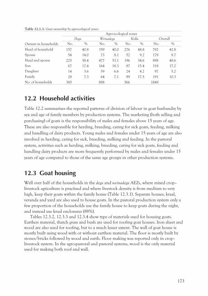
Table 12.1.3. Goat ownership by agro-ecological zones.
Owners in households
Agro-ecological zones
Dega Weinadega Kolla Overall
No. % No. % No. % No. %
Head of household 157 40.8 359 40.0 276 48.8 792 42.8
Spouse 54 14.0 73 8.1 52 9.2 179 9.7
Head and spouse 225 58.4 477 53.1 196 34.6 898 48.6
Son 67 17.4 164 18.3 87 15.4 318 17.2
Daughter 14 3.6 59 6.6 24 4.2 97 5.2
Family 28 7.3 64 7.1 99 17.5 191 10.3
No. of households 385 898 566 1849
12.2 Household activities
Table 12.2 summarises the reported patterns of division of labour in goat husbandry by
sex and age of family members by production systems. The marketing (both selling and
purchasing) of goats is the responsibility of males and females above 15 years of age.
These are also responsible for herding, breeding, caring for sick goats, feeding, milking
and handling of dairy products. Young males and females under 15 years of age are also
involved in herding, caring for sick, breeding, milking and feeding. In the pastoral
system, activities such as herding, milking, breeding, caring for sick goats, feeding and
handling dairy products are more frequently performed by males and females under 15
years of age compared to those of the same age groups in other production systems.
12.3 Goat housingWell over half of the households in the dega and weinadega AEZs, where mixed crop–
livestock agriculture is practised and where livestock density is from medium to very
high, keep their goats within the family house (Table 12.3.1). Separate houses, kraal,
veranda and yard are also used to house goats. In the pastoral production system only a
few proportion of the households use the family house to keep goats during the night,
and instead use kraal enclosures (88%).
Tables 12.3.2, 12.3.3 and 12.3.4 show type of materials used for housing goats.
Earthen material, thatch grass and bush are used for roofing goat houses. Iron sheet and
wood are also used for roofing, but to a much lesser extent. The wall of goat house is
mostly built using wood with or without earthen material. The floor is mostly built by
stones/bricks followed by wood and earth. Floor making was reported only in crop–
livestock system. In the agro-pastoral and pastoral systems, wood is the only material
used for making both roof and wall.
173
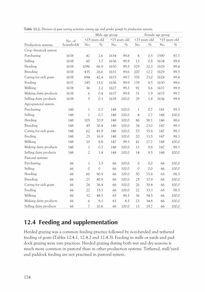
Table 12.2. Division of goat raising activities among age and gender groups by production systems.
Production systemsNo. of
households
Male age group Female age group
<15 years old >15 years old <15 years old >15 years old
No. % No. % No. % No. %
Crop–livestock system
Purchasing 1638 42 2.6 1634 99.8 8 0.5 1590 97.1
Selling 1638 60 3.7 1636 99.9 13 0.8 1634 99.8
Herding 1638 1096 66.9 1630 99.5 529 32.3 1628 99.4
Breeding 1638 435 26.6 1631 99.6 200 12.2 1629 99.5
Caring for sick goats 1638 694 42.4 1633 99.7 376 23.0 1628 99.4
Feeding 1637 245 15.0 1636 99.9 139 8.5 1630 99.6
Milking 1638 36 2.2 1627 99.3 92 5.6 1637 99.9
Making dairy products 1638 6 0.4 1637 99.9 31 1.9 1633 99.7
Selling dairy products 1638 5 0.3 1638 100.0 29 1.8 1636 99.9
Agro-pastoral system
Purchasing 148 1 0.7 148 100.0 1 0.7 141 95.3
Selling 148 1 0.7 148 100.0 4 2.7 148 100.0
Herding 148 105 70.9 148 100.0 86 58.1 146 98.6
Breeding 148 45 30.4 148 100.0 34 23.0 147 99.3
Caring for sick goats 148 62 41.9 148 100.0 53 35.8 147 99.3
Feeding 148 25 16.9 148 100.0 20 13.5 147 99.3
Milking 148 10 6.8 147 99.3 41 27.7 148 100.0
Making dairy products 148 1 0.7 148 100.0 13 8.8 147 99.3
Selling dairy products 148 2 1.4 148 100.0 14 9.5 148 100.0
Pastoral systems
Purchasing 66 1 1.5 66 100.0 0 0.0 66 100.0
Selling 66 0 0 66 100.0 0 0.0 66 100.0
Herding 66 60 90.9 66 100.0 50 75.8 65 98.5
Breeding 66 27 40.9 66 100.0 25 37.9 66 100.0
Caring for sick goats 66 24 36.4 66 100.0 26 39.4 66 100.0
Feeding 66 22 33.3 66 100.0 22 33.3 65 98.5
Milking 66 32 48.5 65 98.5 36 54.5 66 100.0
Making dairy products 66 6 9.1 65 8.5 23 34.8 66 100.0
Selling dairy products 66 7 10.6 66 100.0 13 19.7 66 100.0
12.4 Feeding and supplementationHerded grazing was a common feeding practice followed by non-herded and tethered
feeding of goats (Tables 12.4.1, 12.4.2 and 12.4.3). Feeding in stalls or yards and pad-
dock grazing were rare practices. Herded grazing during both wet and dry seasons is
much more common in pastoral than in other production systems. Tethered, stall/yard
and paddock feeding are not practised in pastoral system.
174
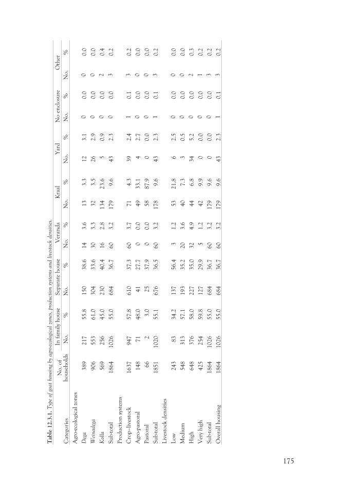
175
Tab
le12.3
.1.
Typ
eof
goat
hou
sing
byagr
o-ec
olog
icalzo
nes
,pro
duct
ion
syst
ems
and
live
stoc
kden
siti
es.
Cat
ego
ries
No
.o
fh
ou
seh
old
s
Infa
mil
yh
ou
seS
epar
ate
ho
use
Ver
and
aK
raal
Yar
dN
oen
clo
sure
Oth
er
No
.%
No
.%
No
.%
No
.%
No
.%
No
.%
No
.%
Agr
o-e
colo
gica
lzo
nes
Deg
a389
217
55.8
150
38.6
14
3.6
13
3.3
12
3.1
00.0
00.0
Wei
nadeg
a906
553
61.0
304
33.6
30
3.3
32
3.5
26
2.9
00.0
00.0
Kol
la569
256
45.0
230
40.4
16
2.8
134
23.6
50.9
00.0
20.4
Su
b-to
tal
1864
1026
55.0
684
36.7
60
3.2
179
9.6
43
2.3
00.0
30.2
Pro
du
ctio
nsy
stem
s
Cro
p–li
vest
ock
1637
947
57.8
610
37.3
60
3.7
71
4.3
39
2.4
10.1
30.2
Agr
o-p
asto
ral
148
71
48.0
41
27.7
00.0
49
33.1
42.7
00.0
00.0
Pas
tora
l66
23.0
25
37.9
00.0
58
87.9
00.0
00.0
00.0
Su
b-to
tal
1851
1020
55.1
676
36.5
60
3.2
178
9.6
43
2.3
10.1
30.2
Liv
esto
ckd
ensi
ties
Lo
w243
83
34.2
137
56.4
31.2
53
21.8
62.5
00.0
00.0
Med
ium
548
313
57.1
193
35.2
20
3.6
40
7.3
30.5
00.0
00.0
Hig
h648
376
58.0
227
35.0
32
4.9
44
6.8
34
5.2
00.0
20.3
Ver
yh
igh
425
254
59.8
127
29.9
51.2
42
9.9
00.0
00.0
10.2
Su
b-to
tal
1864
1026
55.0
684
36.7
60
3.2
179
9.6
00.0
00.0
30.2
Ove
rall
ho
usi
ng
1864
1026
55.0
684
36.7
60
3.2
179
9.6
43
2.3
10.1
30.2
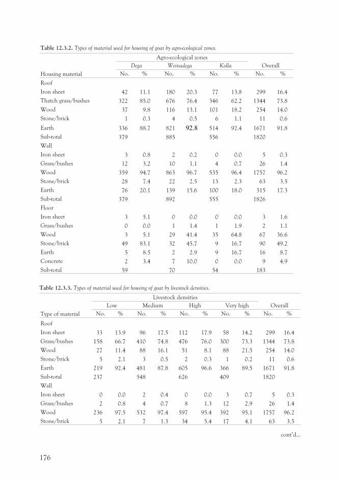
Table 12.3.2. Types of material used for housing of goat by agro-ecological zones.
Housing material
Agro-ecological zones
OverallDega Weinadega Kolla
No. % No. % No. % No. %
Roof
Iron sheet 42 11.1 180 20.3 77 13.8 299 16.4
Thatch grass/bushes 322 85.0 676 76.4 346 62.2 1344 73.8
Wood 37 9.8 116 13.1 101 18.2 254 14.0
Stone/brick 1 0.3 4 0.5 6 1.1 11 0.6
Earth 336 88.7 821 92.8 514 92.4 1671 91.8
Sub-total 379 885 556 1820
Wall
Iron sheet 3 0.8 2 0.2 0 0.0 5 0.3
Grass/bushes 12 3.2 10 1.1 4 0.7 26 1.4
Wood 359 94.7 863 96.7 535 96.4 1757 96.2
Stone/brick 28 7.4 22 2.5 13 2.3 63 3.5
Earth 76 20.1 139 15.6 100 18.0 315 17.3
Sub-total 379 892 555 1826
Floor
Iron sheet 3 5.1 0 0.0 0 0.0 3 1.6
Grass/bushes 0 0.0 1 1.4 1 1.9 2 1.1
Wood 3 5.1 29 41.4 35 64.8 67 36.6
Stone/brick 49 83.1 32 45.7 9 16.7 90 49.2
Earth 5 8.5 2 2.9 9 16.7 16 8.7
Concrete 2 3.4 7 10.0 0 0.0 9 4.9
Sub-total 59 70 54 183
Table 12.3.3. Types of material used for housing of goat by livestock densities.
Type of material
Livestock densities
OverallLow Medium High Very high
No. % No. % No. % No. % No. %
Roof
Iron sheet 33 13.9 96 17.5 112 17.9 58 14.2 299 16.4
Grass/bushes 158 66.7 410 74.8 476 76.0 300 73.3 1344 73.8
Wood 27 11.4 88 16.1 51 8.1 88 21.5 254 14.0
Stone/brick 5 2.1 3 0.5 2 0.3 1 0.2 11 0.6
Earth 219 92.4 481 87.8 605 96.6 366 89.5 1671 91.8
Sub-total 237 548 626 409 1820
Wall
Iron sheet 0 0.0 2 0.4 0 0.0 3 0.7 5 0.3
Grass/bushes 2 0.8 4 0.7 8 1.3 12 2.9 26 1.4
Wood 236 97.5 532 97.4 597 95.4 392 95.1 1757 96.2
Stone/brick 5 2.1 7 1.3 34 5.4 17 4.1 63 3.5
176
cont’d...
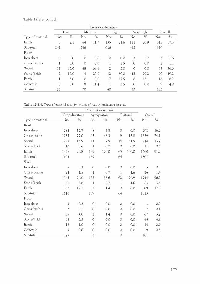
Type of material
Livestock densities
OverallLow Medium High Very high
No. % No. % No. % No. % No. %
Earth 5 2.1 64 11.7 135 21.6 111 26.9 315 17.3
Sub-total 242 546 626 412 1826
Floor
Iron sheet 0 0.0 0 0.0 0 0.0 3 5.7 3 1.6
Grass/bushes 1 5.0 0 0.0 1 2.5 0 0.0 2 1.1
Wood 17 85.0 48 68.6 2 5.0 0 0.0 67 36.6
Stone/brick 2 10.0 14 20.0 32 80.0 42 79.2 90 49.2
Earth 1 5.0 0 0.0 7 17.5 8 15.1 16 8.7
Concrete 0 0.0 8 11.4 1 2.5 0 0.0 9 4.9
Sub-total 20 70 40 53 183
Table 12.3.4. Types of material used for housing of goat by production systems.
Type of material
Production systems
OverallCrop–livestock Agro-pastoral Pastoral
No. % No. % No. % No. %
Roof
Iron sheet 284 17.7 8 5.8 0 0.0 292 16.2
Grass/bushes 1235 77.0 95 68.3 9 13.8 1339 74.1
Wood 223 13.9 11 7.9 14 21.5 248 13.7
Stone/brick 10 0.6 1 0.7 0 0.0 11 0.6
Earth 1456 90.8 139 100.0 65 100.0 1660 91.9
Sub-total 1603 139 65 1807
Wall
Iron sheet 5 0.3 0 0.0 0 0.0 5 0.3
Grass/bushes 24 1.5 1 0.7 1 1.6 26 1.4
Wood 1545 96.0 137 98.6 62 96.9 1744 96.2
Stone/brick 61 3.8 1 0.7 1 1.6 63 3.5
Earth 307 19.1 2 1.4 0 0.0 309 17.0
Sub-total 1610 139 64 1813
Floor
Iron sheet 3 0.2 0 0.0 0 0.0 3 0.2
Grass/bushes 2 0.1 0 0.0 0 0.0 2 0.1
Wood 65 4.0 2 1.4 0 0.0 67 3.7
Stone/brick 88 5.5 0 0.0 0 0.0 88 4.9
Earth 16 1.0 0 0.0 0 0.0 16 0.9
Concrete 9 0.6 0 0.0 0 0.0 9 0.5
Sub-total 179 2 0 181
177
Table 12.3.3. cont’d.
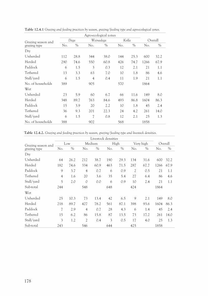
Table 12.4.1 Grazing and feeding practices by season, grazing/feeding type and agro-ecological zones.
Grazing season andgrazing type
Agro-ecological zones
OverallDega Weinadega Kolla
No. % No. % No. % No. %
Dry
Unherded 112 28.8 344 38.0 144 25.3 600 32.2
Herded 290 74.6 550 60.8 426 74.7 1266 67.9
Paddock 6 1.5 3 0.3 12 2.1 21 1.1
Tethered 13 3.3 63 7.0 10 1.8 86 4.6
Stall/yard 6 1.5 4 0.4 11 1.9 21 1.1
No. of households 389 905 570 1864
Wet
Unherded 23 5.9 60 6.7 66 11.6 149 8.0
Herded 348 89.7 763 84.6 493 86.8 1604 86.3
Paddock 15 3.9 20 2.2 10 1.8 45 2.4
Tethered 36 9.3 201 22.3 24 4.2 261 14.0
Stall/yard 6 1.5 7 0.8 12 2.1 25 1.3
No. of households 388 902 568 1858
Table 12.4.2. Grazing and feeding practices by season, grazing/feeding type and livestock densities.
Grazing season andgrazing type
Livestock densities
OverallLow Medium High Very high
No. % No. % No. % No. % No. %
Dry
Unherded 64 26.2 212 38.7 190 29.3 134 31.6 600 32.2
Herded 182 74.6 334 60.9 463 71.5 287 67.7 1266 67.9
Paddock 9 3.7 4 0.7 6 0.9 2 0.5 21 1.1
Tethered 4 1.6 20 3.6 35 5.4 27 6.4 86 4.6
Stall/yard 5 2.0 0 0.0 6 0.9 10 2.4 21 1.1
Sub-total 244 548 648 424 1864
Wet
Unherded 25 10.3 73 13.4 42 6.5 9 2.1 149 8.0
Herded 218 89.7 427 78.2 561 87.1 398 93.6 1604 86.3
Paddock 7 2.9 4 0.7 28 4.3 6 1.4 45 2.4
Tethered 15 6.2 86 15.8 87 13.5 73 17.2 261 14.0
Stall/yard 3 1.2 2 0.4 3 0.5 17 4.0 25 1.3
Sub-total 243 546 644 425 1858
178
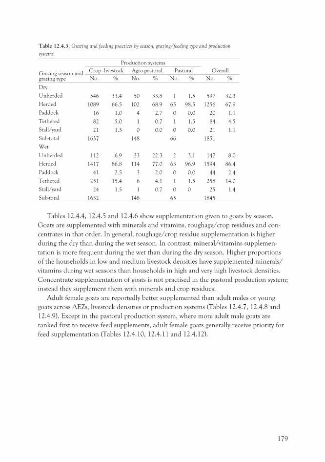
Table 12.4.3. Grazing and feeding practices by season, grazing/feeding type and production
systems.
Grazing season andgrazing type
Production systems
OverallCrop–livestock Agro-pastoral Pastoral
No. % No. % No. % No. %
Dry
Unherded 546 33.4 50 33.8 1 1.5 597 32.3
Herded 1089 66.5 102 68.9 65 98.5 1256 67.9
Paddock 16 1.0 4 2.7 0 0.0 20 1.1
Tethered 82 5.0 1 0.7 1 1.5 84 4.5
Stall/yard 21 1.3 0 0.0 0 0.0 21 1.1
Sub-total 1637 148 66 1851
Wet
Unherded 112 6.9 33 22.3 2 3.1 147 8.0
Herded 1417 86.8 114 77.0 63 96.9 1594 86.4
Paddock 41 2.5 3 2.0 0 0.0 44 2.4
Tethered 251 15.4 6 4.1 1 1.5 258 14.0
Stall/yard 24 1.5 1 0.7 0 0 25 1.4
Sub-total 1632 148 65 1845
Tables 12.4.4, 12.4.5 and 12.4.6 show supplementation given to goats by season.
Goats are supplemented with minerals and vitamins, roughage/crop residues and con-
centrates in that order. In general, roughage/crop residue supplementation is higher
during the dry than during the wet season. In contrast, mineral/vitamins supplemen-
tation is more frequent during the wet than during the dry season. Higher proportions
of the households in low and medium livestock densities have supplemented minerals/
vitamins during wet seasons than households in high and very high livestock densities.
Concentrate supplementation of goats is not practised in the pastoral production system;
instead they supplement them with minerals and crop residues.
Adult female goats are reportedly better supplemented than adult males or young
goats across AEZs, livestock densities or production systems (Tables 12.4.7, 12.4.8 and
12.4.9). Except in the pastoral production system, where more adult male goats are
ranked first to receive feed supplements, adult female goats generally receive priority for
feed supplementation (Tables 12.4.10, 12.4.11 and 12.4.12).
179
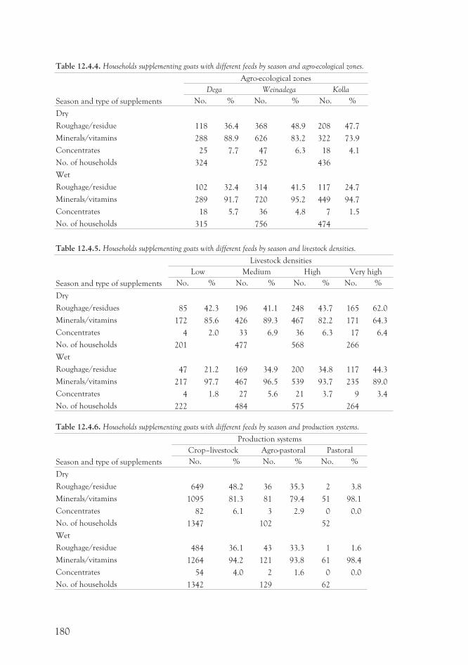
Table 12.4.4. Households supplementing goats with different feeds by season and agro-ecological zones.
Season and type of supplements
Agro-ecological zones
Dega Weinadega Kolla
No. % No. % No. %
Dry
Roughage/residue 118 36.4 368 48.9 208 47.7
Minerals/vitamins 288 88.9 626 83.2 322 73.9
Concentrates 25 7.7 47 6.3 18 4.1
No. of households 324 752 436
Wet
Roughage/residue 102 32.4 314 41.5 117 24.7
Minerals/vitamins 289 91.7 720 95.2 449 94.7
Concentrates 18 5.7 36 4.8 7 1.5
No. of households 315 756 474
Table 12.4.5. Households supplementing goats with different feeds by season and livestock densities.
Season and type of supplements
Livestock densities
Low Medium High Very high
No. % No. % No. % No. %
Dry
Roughage/residues 85 42.3 196 41.1 248 43.7 165 62.0
Minerals/vitamins 172 85.6 426 89.3 467 82.2 171 64.3
Concentrates 4 2.0 33 6.9 36 6.3 17 6.4
No. of households 201 477 568 266
Wet
Roughage/residue 47 21.2 169 34.9 200 34.8 117 44.3
Minerals/vitamins 217 97.7 467 96.5 539 93.7 235 89.0
Concentrates 4 1.8 27 5.6 21 3.7 9 3.4
No. of households 222 484 575 264
Table 12.4.6. Households supplementing goats with different feeds by season and production systems.
Season and type of supplements
Production systems
Crop–livestock Agro-pastoral Pastoral
No. % No. % No. %
Dry
Roughage/residue 649 48.2 36 35.3 2 3.8
Minerals/vitamins 1095 81.3 81 79.4 51 98.1
Concentrates 82 6.1 3 2.9 0 0.0
No. of households 1347 102 52
Wet
Roughage/residue 484 36.1 43 33.3 1 1.6
Minerals/vitamins 1264 94.2 121 93.8 61 98.4
Concentrates 54 4.0 2 1.6 0 0.0
No. of households 1342 129 62
180
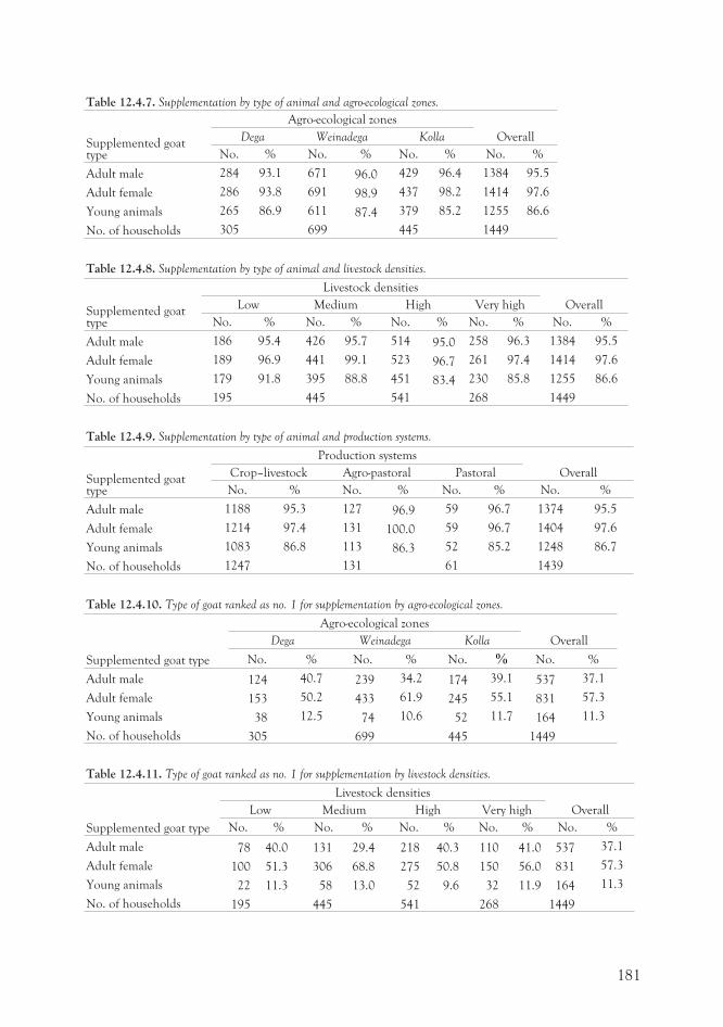
Table 12.4.7. Supplementation by type of animal and agro-ecological zones.
Supplemented goattype
Agro-ecological zones
OverallDega Weinadega Kolla
No. % No. % No. % No. %
Adult male 284 93.1 671 96.0 429 96.4 1384 95.5
Adult female 286 93.8 691 98.9 437 98.2 1414 97.6
Young animals 265 86.9 611 87.4 379 85.2 1255 86.6
No. of households 305 699 445 1449
Table 12.4.8. Supplementation by type of animal and livestock densities.
Supplemented goattype
Livestock densities
OverallLow Medium High Very high
No. % No. % No. % No. % No. %
Adult male 186 95.4 426 95.7 514 95.0 258 96.3 1384 95.5
Adult female 189 96.9 441 99.1 523 96.7 261 97.4 1414 97.6
Young animals 179 91.8 395 88.8 451 83.4 230 85.8 1255 86.6
No. of households 195 445 541 268 1449
Table 12.4.9. Supplementation by type of animal and production systems.
Supplemented goattype
Production systems
OverallCrop–livestock Agro-pastoral Pastoral
No. % No. % No. % No. %
Adult male 1188 95.3 127 96.9 59 96.7 1374 95.5
Adult female 1214 97.4 131 100.0 59 96.7 1404 97.6
Young animals 1083 86.8 113 86.3 52 85.2 1248 86.7
No. of households 1247 131 61 1439
Table 12.4.10. Type of goat ranked as no. 1 for supplementation by agro-ecological zones.
Supplemented goat type
Agro-ecological zones
OverallDega Weinadega Kolla
No. % No. % No. % No. %
Adult male 124 40.7 239 34.2 174 39.1 537 37.1
Adult female 153 50.2 433 61.9 245 55.1 831 57.3
Young animals 38 12.5 74 10.6 52 11.7 164 11.3
No. of households 305 699 445 1449
Table 12.4.11. Type of goat ranked as no. 1 for supplementation by livestock densities.
Supplemented goat type
Livestock densities
OverallLow Medium High Very high
No. % No. % No. % No. % No. %
Adult male 78 40.0 131 29.4 218 40.3 110 41.0 537 37.1
Adult female 100 51.3 306 68.8 275 50.8 150 56.0 831 57.3
Young animals 22 11.3 58 13.0 52 9.6 32 11.9 164 11.3
No. of households 195 445 541 268 1449
181
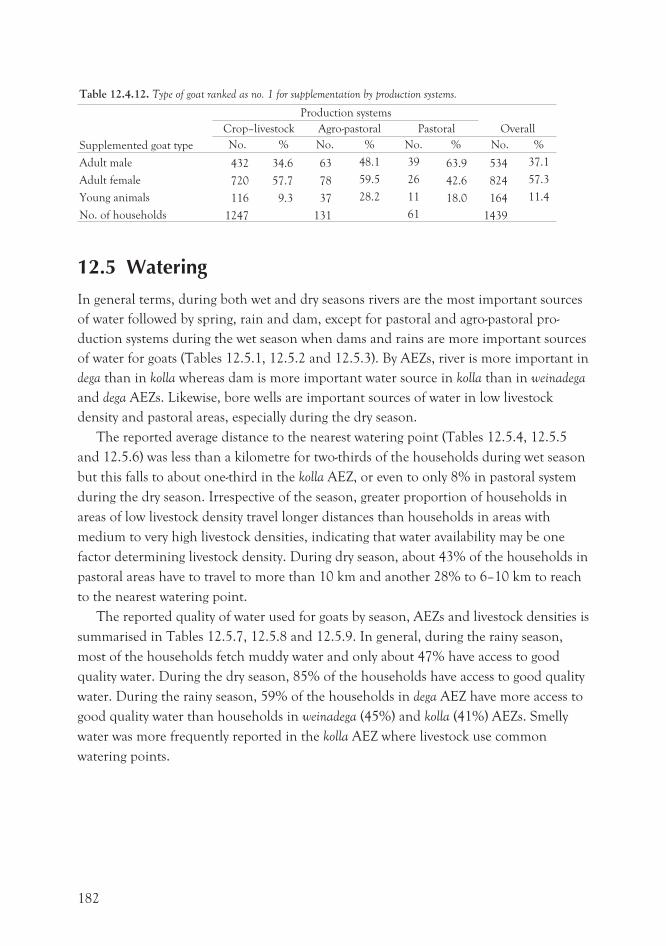
Table 12.4.12. Type of goat ranked as no. 1 for supplementation by production systems.
Supplemented goat type
Production systems
OverallCrop–livestock Agro-pastoral Pastoral
No. % No. % No. % No. %
Adult male 432 34.6 63 48.1 39 63.9 534 37.1
Adult female 720 57.7 78 59.5 26 42.6 824 57.3
Young animals 116 9.3 37 28.2 11 18.0 164 11.4
No. of households 1247 131 61 1439
12.5 Watering
In general terms, during both wet and dry seasons rivers are the most important sources
of water followed by spring, rain and dam, except for pastoral and agro-pastoral pro-
duction systems during the wet season when dams and rains are more important sources
of water for goats (Tables 12.5.1, 12.5.2 and 12.5.3). By AEZs, river is more important in
dega than in kolla whereas dam is more important water source in kolla than in weinadega
and dega AEZs. Likewise, bore wells are important sources of water in low livestock
density and pastoral areas, especially during the dry season.
The reported average distance to the nearest watering point (Tables 12.5.4, 12.5.5
and 12.5.6) was less than a kilometre for two-thirds of the households during wet season
but this falls to about one-third in the kolla AEZ, or even to only 8% in pastoral system
during the dry season. Irrespective of the season, greater proportion of households in
areas of low livestock density travel longer distances than households in areas with
medium to very high livestock densities, indicating that water availability may be one
factor determining livestock density. During dry season, about 43% of the households in
pastoral areas have to travel to more than 10 km and another 28% to 6–10 km to reach
to the nearest watering point.
The reported quality of water used for goats by season, AEZs and livestock densities is
summarised in Tables 12.5.7, 12.5.8 and 12.5.9. In general, during the rainy season,
most of the households fetch muddy water and only about 47% have access to good
quality water. During the dry season, 85% of the households have access to good quality
water. During the rainy season, 59% of the households in dega AEZ have more access to
good quality water than households in weinadega (45%) and kolla (41%) AEZs. Smelly
water was more frequently reported in the kolla AEZ where livestock use common
watering points.
182
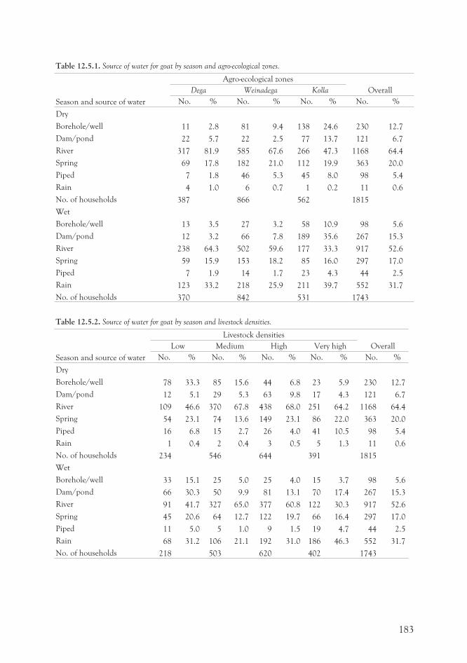
Table 12.5.1. Source of water for goat by season and agro-ecological zones.
Season and source of water
Agro-ecological zones
OverallDega Weinadega Kolla
No. % No. % No. % No. %
Dry
Borehole/well 11 2.8 81 9.4 138 24.6 230 12.7
Dam/pond 22 5.7 22 2.5 77 13.7 121 6.7
River 317 81.9 585 67.6 266 47.3 1168 64.4
Spring 69 17.8 182 21.0 112 19.9 363 20.0
Piped 7 1.8 46 5.3 45 8.0 98 5.4
Rain 4 1.0 6 0.7 1 0.2 11 0.6
No. of households 387 866 562 1815
Wet
Borehole/well 13 3.5 27 3.2 58 10.9 98 5.6
Dam/pond 12 3.2 66 7.8 189 35.6 267 15.3
River 238 64.3 502 59.6 177 33.3 917 52.6
Spring 59 15.9 153 18.2 85 16.0 297 17.0
Piped 7 1.9 14 1.7 23 4.3 44 2.5
Rain 123 33.2 218 25.9 211 39.7 552 31.7
No. of households 370 842 531 1743
Table 12.5.2. Source of water for goat by season and livestock densities.
Season and source of water
Livestock densities
OverallLow Medium High Very high
No. % No. % No. % No. % No. %
Dry
Borehole/well 78 33.3 85 15.6 44 6.8 23 5.9 230 12.7
Dam/pond 12 5.1 29 5.3 63 9.8 17 4.3 121 6.7
River 109 46.6 370 67.8 438 68.0 251 64.2 1168 64.4
Spring 54 23.1 74 13.6 149 23.1 86 22.0 363 20.0
Piped 16 6.8 15 2.7 26 4.0 41 10.5 98 5.4
Rain 1 0.4 2 0.4 3 0.5 5 1.3 11 0.6
No. of households 234 546 644 391 1815
Wet
Borehole/well 33 15.1 25 5.0 25 4.0 15 3.7 98 5.6
Dam/pond 66 30.3 50 9.9 81 13.1 70 17.4 267 15.3
River 91 41.7 327 65.0 377 60.8 122 30.3 917 52.6
Spring 45 20.6 64 12.7 122 19.7 66 16.4 297 17.0
Piped 11 5.0 5 1.0 9 1.5 19 4.7 44 2.5
Rain 68 31.2 106 21.1 192 31.0 186 46.3 552 31.7
No. of households 218 503 620 402 1743
183
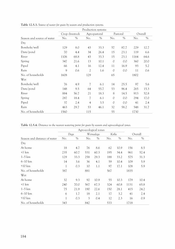
Table 12.5.3. Source of water for goats by season and production systems.
Season and source of water
Production systems
OverallCrop–livestock Agro-pastoral Pastoral
No. % No. % No. % No. %
Dry
Borehole/well 129 8.0 43 33.3 57 87.7 229 12.7
Dam/pond 70 4.4 34 26.4 15 23.1 119 6.6
River 1106 68.8 43 33.3 15 23.1 1164 64.6
Spring 347 21.6 13 10.1 0 0.0 360 20.0
Piped 66 4.1 16 12.4 11 16.9 93 5.2
Rain 9 0.6 2 1.6 0 0.0 11 0.6
No. of households 1608 129 65 1802
Wet
Borehole/well 76 4.9 7 6.1 14 25.5 97 5.6
Dam/pond 148 9.5 64 55.7 53 96.4 265 15.3
River 884 56.7 21 18.3 8 14.5 913 52.8
Spring 287 18.4 7 6.1 0 0.0 294 17.0
Piped 37 2.4 4 3.5 0 0.0 41 2.4
Rain 463 29.7 53 46.1 32 58.2 548 31.7
No. of households 1560 115 55 1730
Table 12.5.4. Distance to the nearest watering point for goats by season and agro-ecological zones.
Season and distance of water
Agro-ecological zones
OverallDega Weinadega Kolla
No. % No. % No. % No. %
Dry
At home 18 4.7 76 8.6 62 10.9 156 8.5
<1 km 235 60.7 531 60.3 195 34.4 961 52.4
1–5 km 129 33.3 258 29.3 188 33.2 575 31.3
6–10 km 14 3.6 36 4.1 59 10.4 109 5.9
>10 km 1 0.3 10 1.1 97 17.1 108 5.9
No. of households 387 881 567 1835
Wet
At home 32 9.3 92 10.9 55 10.3 179 10.4
<1 km 240 70.0 567 67.3 324 60.8 1131 65.8
1–5 km 75 21.9 190 22.6 150 28.1 415 24.2
6–10 km 6 1.7 18 2.1 17 3.2 41 2.4
>10 km 1 0.3 3 0.4 12 2.3 16 0.9
No. of households 343 842 533 1718
184
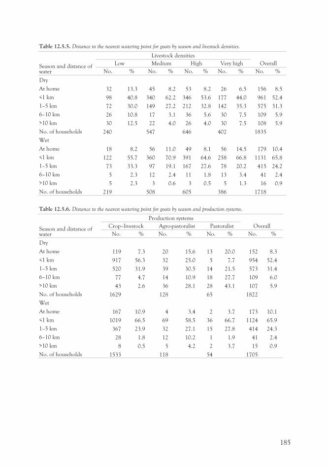
Table 12.5.5. Distance to the nearest watering point for goats by season and livestock densities.
Season and distance ofwater
Livestock densities
OverallLow Medium High Very high
No. % No. % No. % No. % No. %
Dry
At home 32 13.3 45 8.2 53 8.2 26 6.5 156 8.5
<1 km 98 40.8 340 62.2 346 53.6 177 44.0 961 52.4
1–5 km 72 30.0 149 27.2 212 32.8 142 35.3 575 31.3
6–10 km 26 10.8 17 3.1 36 5.6 30 7.5 109 5.9
>10 km 30 12.5 22 4.0 26 4.0 30 7.5 108 5.9
No. of households 240 547 646 402 1835
Wet
At home 18 8.2 56 11.0 49 8.1 56 14.5 179 10.4
<1 km 122 55.7 360 70.9 391 64.6 258 66.8 1131 65.8
1–5 km 73 33.3 97 19.1 167 27.6 78 20.2 415 24.2
6–10 km 5 2.3 12 2.4 11 1.8 13 3.4 41 2.4
>10 km 5 2.3 3 0.6 3 0.5 5 1.3 16 0.9
No. of households 219 508 605 386 1718
Table 12.5.6. Distance to the nearest watering point for goats by season and production systems.
Season and distance ofwater
Production systems
OverallCrop–livestock Agro-pastoralist Pastoralist
No. % No. % No. % No. %
Dry
At home 119 7.3 20 15.6 13 20.0 152 8.3
<1 km 917 56.3 32 25.0 5 7.7 954 52.4
1–5 km 520 31.9 39 30.5 14 21.5 573 31.4
6–10 km 77 4.7 14 10.9 18 27.7 109 6.0
>10 km 43 2.6 36 28.1 28 43.1 107 5.9
No. of households 1629 128 65 1822
Wet
At home 167 10.9 4 3.4 2 3.7 173 10.1
<1 km 1019 66.5 69 58.5 36 66.7 1124 65.9
1–5 km 367 23.9 32 27.1 15 27.8 414 24.3
6–10 km 28 1.8 12 10.2 1 1.9 41 2.4
>10 km 8 0.5 5 4.2 2 3.7 15 0.9
No. of households 1533 118 54 1705
185
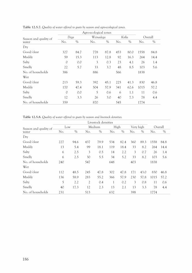
Table 12.5.7. Quality of water offered to goats by season and agro-ecological zones.
Season and quality ofwater
Agro-ecological zones
OverallDega Weinadega Kolla
No. % No. % No. % No. %
Dry
Good/clear 327 84.7 778 87.8 453 80.0 1558 84.8
Muddy 59 15.3 113 12.8 92 16.3 264 14.4
Salty 0 0.0 3 0.3 23 4.1 26 1.4
Smelly 22 5.7 33 3.7 48 8.5 103 5.6
No. of households 386 886 566 1838
Wet
Good/clear 213 59.3 392 45.1 225 41.3 830 46.8
Muddy 170 47.4 504 57.9 341 62.6 1015 57.2
Salty 0 0.0 5 0.6 6 1.1 11 0.6
Smelly 12 3.3 26 3.0 40 7.3 78 4.4
No. of households 359 870 545 1774
Table 12.5.8. Quality of water offered to goats by season and livestock densities.
Season and quality ofwater
Livestock densities
OverallLow Medium High Very high
No. % No. % No. % No. % No. %
Dry
Good/clear 227 94.6 437 79.9 534 82.4 360 89.3 1558 84.8
Muddy 13 5.4 99 18.1 119 18.4 33 8.2 264 14.4
Salty 6 2.5 3 0.5 14 2.2 3 0.7 26 1.4
Smelly 6 2.5 30 5.5 34 5.2 33 8.2 103 5.6
No. of households 240 547 648 403 1838
Wet
Good/clear 112 48.5 245 47.8 302 47.8 171 43.0 830 46.8
Muddy 136 58.9 283 55.2 366 57.9 230 57.8 1015 57.2
Salty 5 2.2 2 0.4 1 0.2 3 0.8 11 0.6
Smelly 40 17.3 12 2.3 13 2.1 13 3.3 78 4.4
No. of households 231 513 632 398 1774
186
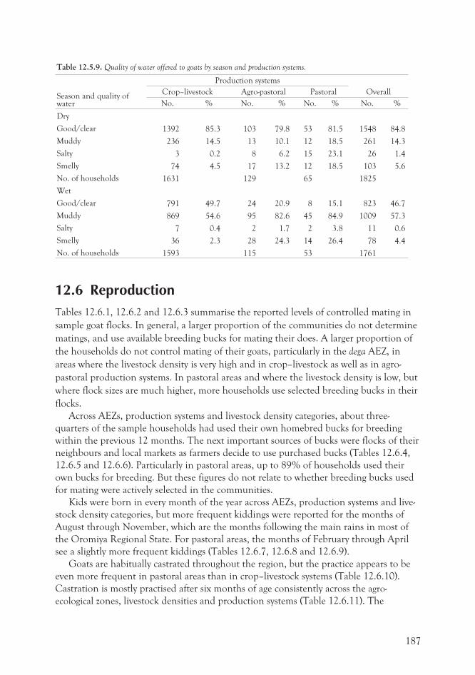
Table 12.5.9. Quality of water offered to goats by season and production systems.
Season and quality ofwater
Production systems
OverallCrop–livestock Agro-pastoral Pastoral
No. % No. % No. % No. %
Dry
Good/clear 1392 85.3 103 79.8 53 81.5 1548 84.8
Muddy 236 14.5 13 10.1 12 18.5 261 14.3
Salty 3 0.2 8 6.2 15 23.1 26 1.4
Smelly 74 4.5 17 13.2 12 18.5 103 5.6
No. of households 1631 129 65 1825
Wet
Good/clear 791 49.7 24 20.9 8 15.1 823 46.7
Muddy 869 54.6 95 82.6 45 84.9 1009 57.3
Salty 7 0.4 2 1.7 2 3.8 11 0.6
Smelly 36 2.3 28 24.3 14 26.4 78 4.4
No. of households 1593 115 53 1761
12.6 ReproductionTables 12.6.1, 12.6.2 and 12.6.3 summarise the reported levels of controlled mating in
sample goat flocks. In general, a larger proportion of the communities do not determine
matings, and use available breeding bucks for mating their does. A larger proportion of
the households do not control mating of their goats, particularly in the dega AEZ, in
areas where the livestock density is very high and in crop–livestock as well as in agro-
pastoral production systems. In pastoral areas and where the livestock density is low, but
where flock sizes are much higher, more households use selected breeding bucks in their
flocks.
Across AEZs, production systems and livestock density categories, about three-
quarters of the sample households had used their own homebred bucks for breeding
within the previous 12 months. The next important sources of bucks were flocks of their
neighbours and local markets as farmers decide to use purchased bucks (Tables 12.6.4,
12.6.5 and 12.6.6). Particularly in pastoral areas, up to 89% of households used their
own bucks for breeding. But these figures do not relate to whether breeding bucks used
for mating were actively selected in the communities.
Kids were born in every month of the year across AEZs, production systems and live-
stock density categories, but more frequent kiddings were reported for the months of
August through November, which are the months following the main rains in most of
the Oromiya Regional State. For pastoral areas, the months of February through April
see a slightly more frequent kiddings (Tables 12.6.7, 12.6.8 and 12.6.9).
Goats are habitually castrated throughout the region, but the practice appears to be
even more frequent in pastoral areas than in crop–livestock systems (Table 12.6.10).
Castration is mostly practised after six months of age consistently across the agro-
ecological zones, livestock densities and production systems (Table 12.6.11). The
187
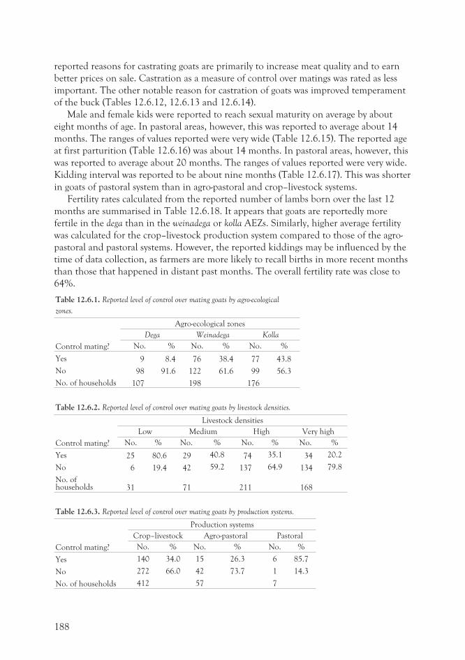
reported reasons for castrating goats are primarily to increase meat quality and to earn
better prices on sale. Castration as a measure of control over matings was rated as less
important. The other notable reason for castration of goats was improved temperament
of the buck (Tables 12.6.12, 12.6.13 and 12.6.14).
Male and female kids were reported to reach sexual maturity on average by about
eight months of age. In pastoral areas, however, this was reported to average about 14
months. The ranges of values reported were very wide (Table 12.6.15). The reported age
at first parturition (Table 12.6.16) was about 14 months. In pastoral areas, however, this
was reported to average about 20 months. The ranges of values reported were very wide.
Kidding interval was reported to be about nine months (Table 12.6.17). This was shorter
in goats of pastoral system than in agro-pastoral and crop–livestock systems.
Fertility rates calculated from the reported number of lambs born over the last 12
months are summarised in Table 12.6.18. It appears that goats are reportedly more
fertile in the dega than in the weinadega or kolla AEZs. Similarly, higher average fertility
was calculated for the crop–livestock production system compared to those of the agro-
pastoral and pastoral systems. However, the reported kiddings may be influenced by the
time of data collection, as farmers are more likely to recall births in more recent months
than those that happened in distant past months. The overall fertility rate was close to
64%.
Table 12.6.1. Reported level of control over mating goats by agro-ecological
zones.
Control mating?
Agro-ecological zones
Dega Weinadega Kolla
No. % No. % No. %
Yes 9 8.4 76 38.4 77 43.8
No 98 91.6 122 61.6 99 56.3
No. of households 107 198 176
Table 12.6.2. Reported level of control over mating goats by livestock densities.
Control mating?
Livestock densities
Low Medium High Very high
No. % No. % No. % No. %
Yes 25 80.6 29 40.8 74 35.1 34 20.2
No 6 19.4 42 59.2 137 64.9 134 79.8
No. ofhouseholds 31 71 211 168
Table 12.6.3. Reported level of control over mating goats by production systems.
Control mating?
Production systems
Crop–livestock Agro-pastoral Pastoral
No. % No. % No. %
Yes 140 34.0 15 26.3 6 85.7
No 272 66.0 42 73.7 1 14.3
No. of households 412 57 7
188
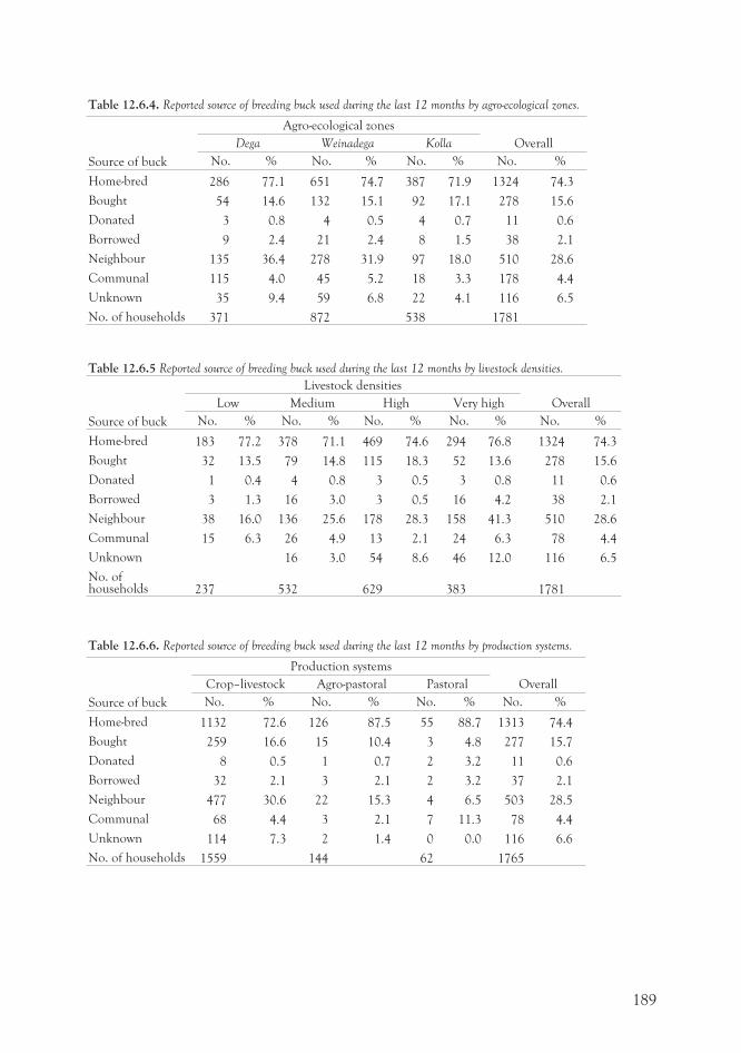
Table 12.6.4. Reported source of breeding buck used during the last 12 months by agro-ecological zones.
Source of buck
Agro-ecological zones
OverallDega Weinadega Kolla
No. % No. % No. % No. %
Home-bred 286 77.1 651 74.7 387 71.9 1324 74.3
Bought 54 14.6 132 15.1 92 17.1 278 15.6
Donated 3 0.8 4 0.5 4 0.7 11 0.6
Borrowed 9 2.4 21 2.4 8 1.5 38 2.1
Neighbour 135 36.4 278 31.9 97 18.0 510 28.6
Communal 115 4.0 45 5.2 18 3.3 178 4.4
Unknown 35 9.4 59 6.8 22 4.1 116 6.5
No. of households 371 872 538 1781
Table 12.6.5 Reported source of breeding buck used during the last 12 months by livestock densities.
Source of buck
Livestock densities
OverallLow Medium High Very high
No. % No. % No. % No. % No. %
Home-bred 183 77.2 378 71.1 469 74.6 294 76.8 1324 74.3
Bought 32 13.5 79 14.8 115 18.3 52 13.6 278 15.6
Donated 1 0.4 4 0.8 3 0.5 3 0.8 11 0.6
Borrowed 3 1.3 16 3.0 3 0.5 16 4.2 38 2.1
Neighbour 38 16.0 136 25.6 178 28.3 158 41.3 510 28.6
Communal 15 6.3 26 4.9 13 2.1 24 6.3 78 4.4
Unknown 16 3.0 54 8.6 46 12.0 116 6.5
No. ofhouseholds 237 532 629 383 1781
Table 12.6.6. Reported source of breeding buck used during the last 12 months by production systems.
Source of buck
Production systems
OverallCrop–livestock Agro-pastoral Pastoral
No. % No. % No. % No. %
Home-bred 1132 72.6 126 87.5 55 88.7 1313 74.4
Bought 259 16.6 15 10.4 3 4.8 277 15.7
Donated 8 0.5 1 0.7 2 3.2 11 0.6
Borrowed 32 2.1 3 2.1 2 3.2 37 2.1
Neighbour 477 30.6 22 15.3 4 6.5 503 28.5
Communal 68 4.4 3 2.1 7 11.3 78 4.4
Unknown 114 7.3 2 1.4 0 0.0 116 6.6
No. of households 1559 144 62 1765
189
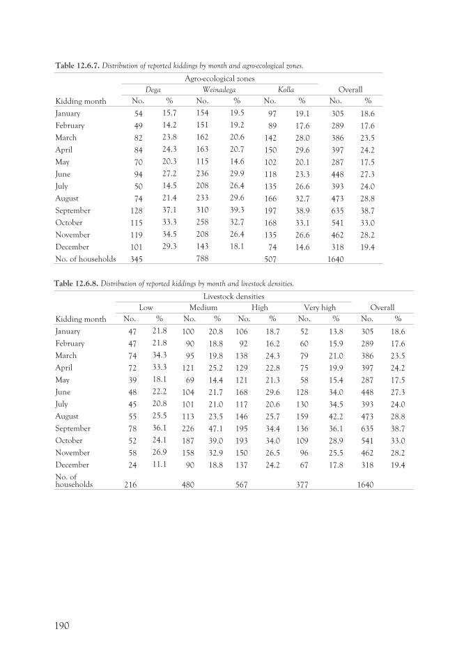
Table 12.6.7. Distribution of reported kiddings by month and agro-ecological zones.
Kidding month
Agro-ecological zones
OverallDega Weinadega Kolla
No. % No. % No. % No. %
January 54 15.7 154 19.5 97 19.1 305 18.6
February 49 14.2 151 19.2 89 17.6 289 17.6
March 82 23.8 162 20.6 142 28.0 386 23.5
April 84 24.3 163 20.7 150 29.6 397 24.2
May 70 20.3 115 14.6 102 20.1 287 17.5
June 94 27.2 236 29.9 118 23.3 448 27.3
July 50 14.5 208 26.4 135 26.6 393 24.0
August 74 21.4 233 29.6 166 32.7 473 28.8
September 128 37.1 310 39.3 197 38.9 635 38.7
October 115 33.3 258 32.7 168 33.1 541 33.0
November 119 34.5 208 26.4 135 26.6 462 28.2
December 101 29.3 143 18.1 74 14.6 318 19.4
No. of households 345 788 507 1640
Table 12.6.8. Distribution of reported kiddings by month and livestock densities.
Kidding month
Livestock densities
OverallLow Medium High Very high
No. % No. % No. % No. % No. %
January 47 21.8 100 20.8 106 18.7 52 13.8 305 18.6
February 47 21.8 90 18.8 92 16.2 60 15.9 289 17.6
March 74 34.3 95 19.8 138 24.3 79 21.0 386 23.5
April 72 33.3 121 25.2 129 22.8 75 19.9 397 24.2
May 39 18.1 69 14.4 121 21.3 58 15.4 287 17.5
June 48 22.2 104 21.7 168 29.6 128 34.0 448 27.3
July 45 20.8 101 21.0 117 20.6 130 34.5 393 24.0
August 55 25.5 113 23.5 146 25.7 159 42.2 473 28.8
September 78 36.1 226 47.1 195 34.4 136 36.1 635 38.7
October 52 24.1 187 39.0 193 34.0 109 28.9 541 33.0
November 58 26.9 158 32.9 150 26.5 96 25.5 462 28.2
December 24 11.1 90 18.8 137 24.2 67 17.8 318 19.4
No. ofhouseholds 216 480 567 377 1640
190
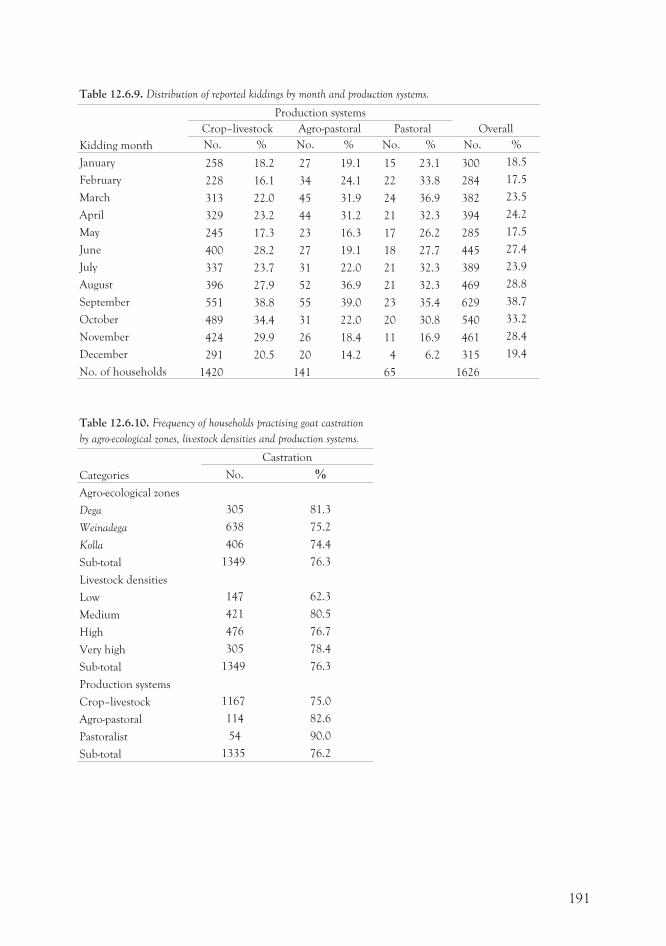
Table 12.6.9. Distribution of reported kiddings by month and production systems.
Kidding month
Production systems
OverallCrop–livestock Agro-pastoral Pastoral
No. % No. % No. % No. %
January 258 18.2 27 19.1 15 23.1 300 18.5
February 228 16.1 34 24.1 22 33.8 284 17.5
March 313 22.0 45 31.9 24 36.9 382 23.5
April 329 23.2 44 31.2 21 32.3 394 24.2
May 245 17.3 23 16.3 17 26.2 285 17.5
June 400 28.2 27 19.1 18 27.7 445 27.4
July 337 23.7 31 22.0 21 32.3 389 23.9
August 396 27.9 52 36.9 21 32.3 469 28.8
September 551 38.8 55 39.0 23 35.4 629 38.7
October 489 34.4 31 22.0 20 30.8 540 33.2
November 424 29.9 26 18.4 11 16.9 461 28.4
December 291 20.5 20 14.2 4 6.2 315 19.4
No. of households 1420 141 65 1626
Table 12.6.10. Frequency of households practising goat castration
by agro-ecological zones, livestock densities and production systems.
Categories
Castration
No. %
Agro-ecological zones
Dega 305 81.3
Weinadega 638 75.2
Kolla 406 74.4
Sub-total 1349 76.3
Livestock densities
Low 147 62.3
Medium 421 80.5
High 476 76.7
Very high 305 78.4
Sub-total 1349 76.3
Production systems
Crop–livestock 1167 75.0
Agro-pastoral 114 82.6
Pastoralist 54 90.0
Sub-total 1335 76.2
191
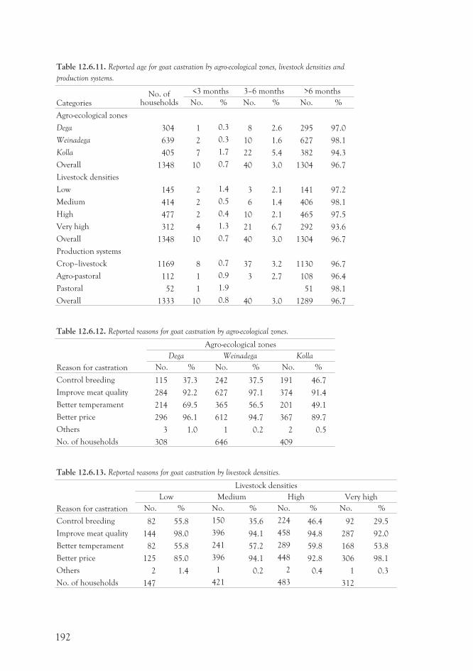
Table 12.6.11. Reported age for goat castration by agro-ecological zones, livestock densities and
production systems.
CategoriesNo. of
households
<3 months 3–6 months >6 months
No. % No. % No. %
Agro-ecological zones
Dega 304 1 0.3 8 2.6 295 97.0
Weinadega 639 2 0.3 10 1.6 627 98.1
Kolla 405 7 1.7 22 5.4 382 94.3
Overall 1348 10 0.7 40 3.0 1304 96.7
Livestock densities
Low 145 2 1.4 3 2.1 141 97.2
Medium 414 2 0.5 6 1.4 406 98.1
High 477 2 0.4 10 2.1 465 97.5
Very high 312 4 1.3 21 6.7 292 93.6
Overall 1348 10 0.7 40 3.0 1304 96.7
Production systems
Crop–livestock 1169 8 0.7 37 3.2 1130 96.7
Agro-pastoral 112 1 0.9 3 2.7 108 96.4
Pastoral 52 1 1.9 51 98.1
Overall 1333 10 0.8 40 3.0 1289 96.7
Table 12.6.12. Reported reasons for goat castration by agro-ecological zones.
Reason for castration
Agro-ecological zones
Dega Weinadega Kolla
No. % No. % No. %
Control breeding 115 37.3 242 37.5 191 46.7
Improve meat quality 284 92.2 627 97.1 374 91.4
Better temperament 214 69.5 365 56.5 201 49.1
Better price 296 96.1 612 94.7 367 89.7
Others 3 1.0 1 0.2 2 0.5
No. of households 308 646 409
Table 12.6.13. Reported reasons for goat castration by livestock densities.
Reason for castration
Livestock densities
Low Medium High Very high
No. % No. % No. % No. %
Control breeding 82 55.8 150 35.6 224 46.4 92 29.5
Improve meat quality 144 98.0 396 94.1 458 94.8 287 92.0
Better temperament 82 55.8 241 57.2 289 59.8 168 53.8
Better price 125 85.0 396 94.1 448 92.8 306 98.1
Others 2 1.4 1 0.2 2 0.4 1 0.3
No. of households 147 421 483 312
192
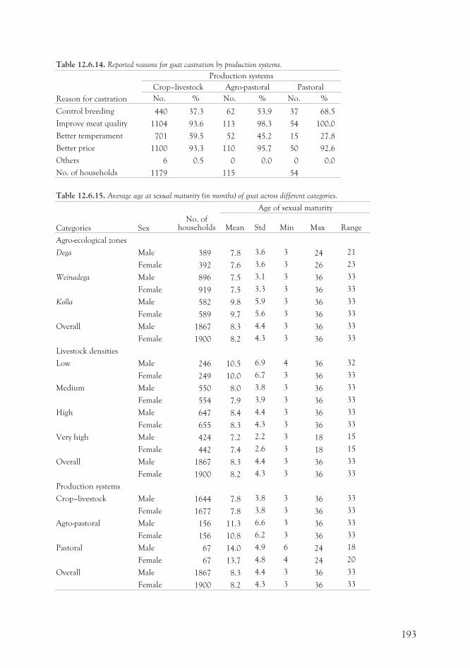
Table 12.6.14. Reported reasons for goat castration by production systems.
Reason for castration
Production systems
Crop–livestock Agro-pastoral Pastoral
No. % No. % No. %
Control breeding 440 37.3 62 53.9 37 68.5
Improve meat quality 1104 93.6 113 98.3 54 100.0
Better temperament 701 59.5 52 45.2 15 27.8
Better price 1100 93.3 110 95.7 50 92.6
Others 6 0.5 0 0.0 0 0.0
No. of households 1179 115 54
Table 12.6.15. Average age at sexual maturity (in months) of goat across different categories.
Categories SexNo. of
households
Age of sexual maturity
Mean Std Min Max Range
Agro-ecological zones
Dega Male 389 7.8 3.6 3 24 21
Female 392 7.6 3.6 3 26 23
Weinadega Male 896 7.5 3.1 3 36 33
Female 919 7.5 3.3 3 36 33
Kolla Male 582 9.8 5.9 3 36 33
Female 589 9.7 5.6 3 36 33
Overall Male 1867 8.3 4.4 3 36 33
Female 1900 8.2 4.3 3 36 33
Livestock densities
Low Male 246 10.5 6.9 4 36 32
Female 249 10.0 6.7 3 36 33
Medium Male 550 8.0 3.8 3 36 33
Female 554 7.9 3.9 3 36 33
High Male 647 8.4 4.4 3 36 33
Female 655 8.3 4.3 3 36 33
Very high Male 424 7.2 2.2 3 18 15
Female 442 7.4 2.6 3 18 15
Overall Male 1867 8.3 4.4 3 36 33
Female 1900 8.2 4.3 3 36 33
Production systems
Crop–livestock Male 1644 7.8 3.8 3 36 33
Female 1677 7.8 3.8 3 36 33
Agro-pastoral Male 156 11.3 6.6 3 36 33
Female 156 10.8 6.2 3 36 33
Pastoral Male 67 14.0 4.9 6 24 18
Female 67 13.7 4.8 4 24 20
Overall Male 1867 8.3 4.4 3 36 33
Female 1900 8.2 4.3 3 36 33
193
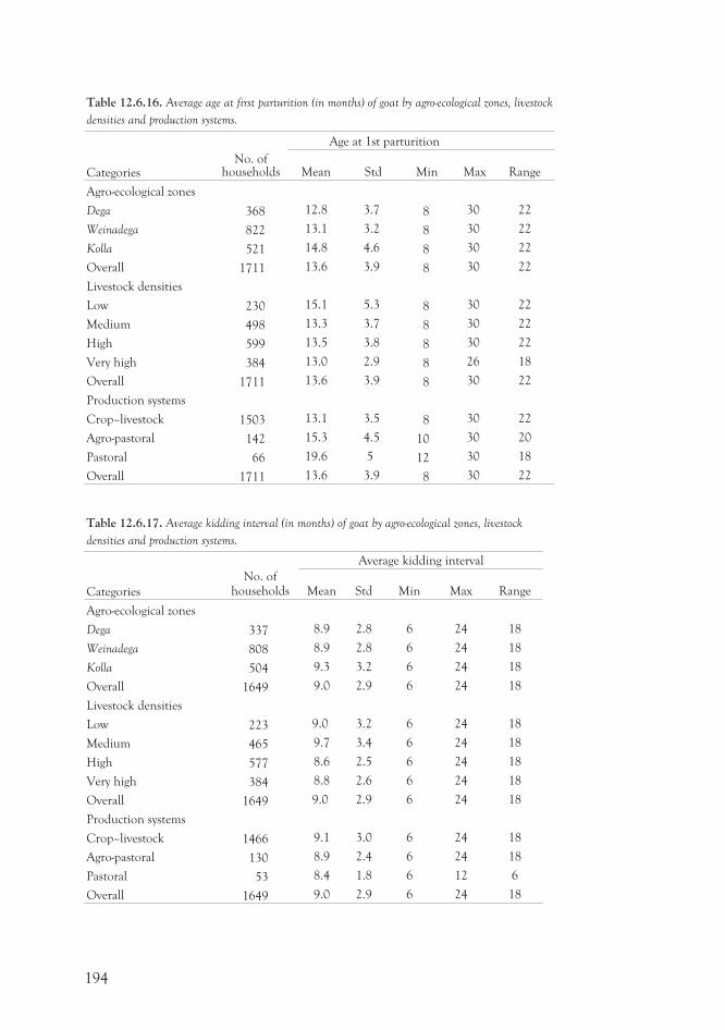
Table 12.6.16. Average age at first parturition (in months) of goat by agro-ecological zones, livestock
densities and production systems.
Categories
Age at 1st parturition
No. ofhouseholds Mean Std Min Max Range
Agro-ecological zones
Dega 368 12.8 3.7 8 30 22
Weinadega 822 13.1 3.2 8 30 22
Kolla 521 14.8 4.6 8 30 22
Overall 1711 13.6 3.9 8 30 22
Livestock densities
Low 230 15.1 5.3 8 30 22
Medium 498 13.3 3.7 8 30 22
High 599 13.5 3.8 8 30 22
Very high 384 13.0 2.9 8 26 18
Overall 1711 13.6 3.9 8 30 22
Production systems
Crop–livestock 1503 13.1 3.5 8 30 22
Agro-pastoral 142 15.3 4.5 10 30 20
Pastoral 66 19.6 5 12 30 18
Overall 1711 13.6 3.9 8 30 22
Table 12.6.17. Average kidding interval (in months) of goat by agro-ecological zones, livestock
densities and production systems.
Categories
No. ofhouseholds
Average kidding interval
Mean Std Min Max Range
Agro-ecological zones
Dega 337 8.9 2.8 6 24 18
Weinadega 808 8.9 2.8 6 24 18
Kolla 504 9.3 3.2 6 24 18
Overall 1649 9.0 2.9 6 24 18
Livestock densities
Low 223 9.0 3.2 6 24 18
Medium 465 9.7 3.4 6 24 18
High 577 8.6 2.5 6 24 18
Very high 384 8.8 2.6 6 24 18
Overall 1649 9.0 2.9 6 24 18
Production systems
Crop–livestock 1466 9.1 3.0 6 24 18
Agro-pastoral 130 8.9 2.4 6 24 18
Pastoral 53 8.4 1.8 6 12 6
Overall 1649 9.0 2.9 6 24 18
194
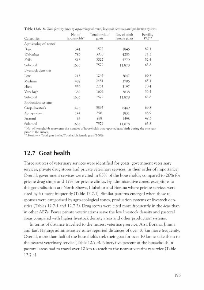
Table 12.6.18. Goat fertility rates by agro-ecological zones, livestock densities and production systems.
CategoriesNo. of
households*Total birth of
goatsNo. of adultfemale goats
Fertility(%)**
Agro-ecological zones
Dega 341 1522 1846 82.4
Weinadega 780 3030 4253 71.2
Kolla 515 3027 5779 52.4
Sub-total 1636 7579 11,878 63.8
Livestock densities
Low 215 1245 2047 60.8
Medium 482 2481 3796 65.4
High 550 2251 3197 70.4
Very high 389 1602 2838 56.4
Sub-total 1636 7579 11,878 63.8
Production systems
Crop–livestock 1426 5895 8449 69.8
Agro-pastoral 144 896 1831 48.9
Pastoral 66 788 1598 49.3
Sub-total 1636 7579 11,878 63.8
* No. of households represents the number of households that reported goat birth during the one yearprior to the survey.** Fertility = Total goat births/Total adult female goats*100%.
12.7 Goat health
Three sources of veterinary services were identified for goats: government veterinary
services, private drug stores and private veterinary services, in their order of importance.
Overall, government services were cited in 85% of the households, compared to 26% for
private drug shops and 12% for private clinics. By administrative zones, exceptions to
this generalisation are North Shewa, Illubabor and Borana where private services were
cited by far more frequently (Table 12.7.1). Similar patterns emerged when these re-
sponses were categorised by agro-ecological zones, production systems or livestock den-
sities (Tables 12.7.1 and 12.7.2). Drug stores were cited more frequently in the dega than
in other AEZs. Fewer private veterinarians serve the low livestock density and pastoral
areas compared with higher livestock density areas and other production systems.
In terms of distance travelled to the nearest veterinary service, Arsi, Borana, Jimma
and East Hararge administrative zones reported distances of over 10 km more frequently.
Overall, more than half of the households trek their goat for over 10 km to take them to
the nearest veterinary service (Table 12.7.3). Ninety-five percent of the households in
pastoral areas had to travel over 10 km to reach to the nearest veterinary service (Table
12.7.4).
195
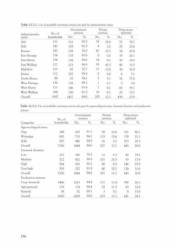
Table 12.7.1. Use of available veterinary services for goat by administrative zones.
Administrativezones
No. ofhouseholds
Governmentservices
Privateservices
Drug stores(private)
No. % No. % No. %
Arsi 131 112 85.5 39 29.8 52 39.7
Bale 141 129 91.5 4 2.8 29 20.6
Borana 183 139 76.0 47 25.7 38 20.8
East Hararge 134 115 85.8 0 0.0 35 26.1
East Shewa 154 138 89.6 14 9.1 30 19.5
East Wellega 127 123 96.9 55 43.3 40 31.5
Illubabor 123 87 70.7 17 13.8 38 30.9
Jimma 112 107 95.5 0 0.0 8 7.1
North Shewa 98 53 54.1 5 5.1 76 77.6
West Hararge 139 138 99.3 1 0.7 5 3.6
West Shewa 171 146 85.4 7 4.1 60 35.1
West Wellega 184 150 81.5 16 8.7 28 15.2
Overall 1697 1437 84.6 205 12.1 439 25.9
Table 12.7.2. Use of available veterinary services for goat by agro-ecological zones, livestock densities and production
systems.
CategoriesNo. of
households
Governmentservices
Privateservices
Drug stores(private)
No. % No. % No. %
Agro-ecological zones
Dega 349 283 81.1 58 16.6 161 46.1
Weinadega 850 715 84.1 133 15.6 179 21.1
Kolla 507 446 88.0 16 3.2 103 20.3
Overall 1706 1444 84.6 207 12.1 443 26.0
Livestock densities
Low 227 180 79.3 12 5.3 80 35.2
Medium 522 422 80.8 107 20.5 93 17.8
High 564 520 92.2 48 8.5 146 25.9
Very high 393 322 81.9 40 10.2 124 31.6
Overall 1706 1444 84.6 207 12.1 443 26.0
Production systems
Crop–livestock 1496 1263 84.4 171 11.4 390 26.1
Agro-pastoral 135 114 84.4 29 21.5 43 31.9
Pastoral 59 52 88.1 3 5.1 8 13.6
Overall 1690 1429 84.6 203 12.1 441 26.1
196
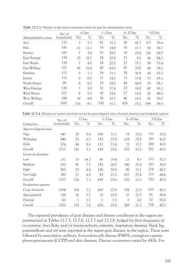
Table 12.7.3. Distance to the nearest veterinary service for goat by administrative zones.
Administrative zonesNo. of
households
<1 km 1–5 km 6–10 km >10 km
No. % No. % No. % No. %
Arsi 131 3 2.3 41 31.3 56 42.7 103 78.6
Bale 141 17 12.1 35 24.8 30 21.3 80 56.7
Borana 183 7 3.8 53 29.0 38 20.8 126 68.9
East Hararge 134 25 18.7 28 20.9 11 8.2 86 64.2
East Shewa 154 7 4.5 34 22.1 51 33.1 89 57.8
East Wellega 127 45 35.4 80 63.0 47 37.0 46 36.2
Ilubabor 123 9 7.3 26 21.1 38 30.9 68 55.3
Jimma 112 0 0.0 27 24.1 15 13.4 73 65.2
North Shewa 98 8 8.2 29 29.6 44 44.9 53 54.1
West Hararge 139 7 5.0 52 37.4 25 18.0 60 43.2
West Shewa 171 9 5.3 95 55.6 27 15.8 82 48.0
West Wellega 184 18 9.8 38 20.7 46 25.0 92 50.0
Overall 1697 155 9.1 538 31.7 428 25.2 958 56.5
Table 12.7.4. Distance to nearest veterinary service by agro-ecological zones, livestock densities and production systems.
CategoriesNo. of
households
<1 km 1–5 km 6–10 km >10 km
No. % No. % No. % No. %
Agro-ecological zones
Dega 347 29 8.4 108 31.1 79 22.8 131 37.8
Weinadega 846 53 6.3 219 25.9 219 25.9 355 42.0
Kolla 524 44 8.4 112 21.4 72 13.7 296 56.5
Overall 1717 126 7.3 439 25.6 370 21.5 782 45.5
Livestock densities
Low 232 33 14.2 45 19.4 21 9.1 133 57.3
Medium 532 41 7.7 143 26.9 146 27.4 202 38.0
High 563 25 4.4 168 29.8 96 17.1 274 48.7
Very high 390 27 6.9 83 21.3 107 27.4 173 44.4
Overall 1717 126 7.3 439 25.6 370 21.5 782 45.5
Production systems
Crop–livestock 1504 108 7.2 419 27.9 338 22.5 639 42.5
Agro-pastoral 138 10 7.2 15 10.9 31 22.5 82 59.4
Pastoral 60 1 1.7 2 3.3 0 0.0 57 95.0
Overall 1702 119 7.0 436 25.6 369 21.7 778 45.7
The reported prevalence of goat diseases and disease conditions in the region are
summarised in Tables 12.7.5, 12.7.6, 12.7.7 and 12.7.8. Judged by their frequency of
occurrence, liver fluke and/or haemonchosis, enteritis, respiratory diseases, black leg,
pasteurellosis and orf were reported as the major goat diseases in the region. These were
followed by emaciation, anthrax, foot-and-mouth disease (FMD), contagious caprine
pleuro-pneumonia (CCPP) and skin diseases. Disease occurrence varied by AEZs. For
197
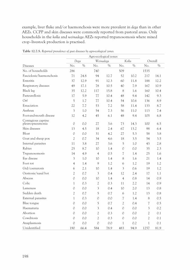
example, liver fluke and/or haemonchosis were more prevalent in dega than in other
AEZs. CCPP and skin diseases were commonly reported from pastoral areas. Only
households in the kolla and weinadega AEZs reported trypanosomosis where mixed
crop–livestock production is practised.
Table 12.7.5. Reported prevalence of goat diseases by agro-ecological zones.
Diseases
Agro-ecological zones
OverallDega Weinadega Kolla
No. % No. % No. % No. %
No. of households 286 740 509 1535
Fasciolosis/haemonchosis 71 24.8 94 12.7 52 10.2 217 14.1
Enteritis 37 12.9 91 12.3 60 11.8 188 12.2
Respiratory diseases 49 17.1 78 10.5 40 7.9 167 10.9
Black leg 35 12.2 117 15.8 8 1.6 160 10.4
Pasteurellosis 17 5.9 77 10.4 48 9.4 142 9.3
Orf 5 1.7 77 10.4 54 10.6 136 8.9
Emaciation 22 7.7 53 7.2 58 11.4 133 8.7
Anthrax 3 1.0 54 7.3 56 11.0 113 7.4
Foot-and-mouth disease 12 4.2 45 6.1 48 9.4 105 6.8
Contagious caprinepleuro-pneumonia 0 0.0 27 3.6 73 14.3 100 6.5
Skin diseases 13 4.5 18 2.4 67 13.2 98 6.4
Bloat 0 0.0 31 4.2 27 5.3 58 3.8
Goat and sheep pox 2 0.7 34 4.6 18 3.5 54 3.5
Internal parasites 11 3.8 27 3.6 5 1.0 43 2.8
Rabies 25 8.7 10 1.4 0 0.0 35 2.3
Trypanosomosis 14 4.9 4 0.5 7 1.4 25 1.6
Eye disease 3 1.0 10 1.4 8 1.6 21 1.4
Foot rot 4 1.4 9 1.2 6 1.2 19 1.2
Gid/coenurosis 6 2.1 10 1.4 3 0.6 19 1.2
Oestrosis/nasal bot 2 0.7 3 0.4 12 2.4 17 1.1
Abscess 0 0.0 10 1.4 4 0.8 14 0.9
Colic 1 0.3 2 0.3 11 2.2 14 0.9
Lameness 0 0.0 3 0.4 10 2.0 13 0.8
Sudden death 2 0.7 5 0.7 6 1.2 13 0.8
External parasites 1 0.3 0 0.0 7 1.4 8 0.5
Blue tongue 0 0.0 5 0.7 2 0.4 7 0.5
Haematuria 0 0.0 3 0.4 0 0.0 3 0.2
Abortion 0 0.0 2 0.3 0 0.0 2 0.1
Cowdriosis 0 0.0 2 0.3 0 0.0 2 0.1
Anaplasmosis 0 0.0 0 0.0 1 0.2 1 0.1
Unidentified 190 66.4 584 78.9 483 94.9 1257 81.9
198
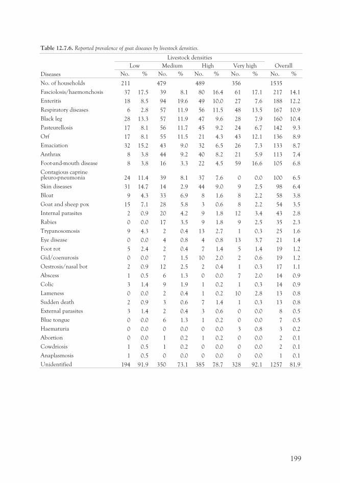
Table 12.7.6. Reported prevalence of goat diseases by livestock densities.
Diseases
Livestock densities
OverallLow Medium High Very high
No. % No. % No. % No. % No. %
No. of households 211 479 489 356 1535
Fasciolosis/haemonchosis 37 17.5 39 8.1 80 16.4 61 17.1 217 14.1
Enteritis 18 8.5 94 19.6 49 10.0 27 7.6 188 12.2
Respiratory diseases 6 2.8 57 11.9 56 11.5 48 13.5 167 10.9
Black leg 28 13.3 57 11.9 47 9.6 28 7.9 160 10.4
Pasteurellosis 17 8.1 56 11.7 45 9.2 24 6.7 142 9.3
Orf 17 8.1 55 11.5 21 4.3 43 12.1 136 8.9
Emaciation 32 15.2 43 9.0 32 6.5 26 7.3 133 8.7
Anthrax 8 3.8 44 9.2 40 8.2 21 5.9 113 7.4
Foot-and-mouth disease 8 3.8 16 3.3 22 4.5 59 16.6 105 6.8
Contagious caprinepleuro-pneumonia 24 11.4 39 8.1 37 7.6 0 0.0 100 6.5
Skin diseases 31 14.7 14 2.9 44 9.0 9 2.5 98 6.4
Bloat 9 4.3 33 6.9 8 1.6 8 2.2 58 3.8
Goat and sheep pox 15 7.1 28 5.8 3 0.6 8 2.2 54 3.5
Internal parasites 2 0.9 20 4.2 9 1.8 12 3.4 43 2.8
Rabies 0 0.0 17 3.5 9 1.8 9 2.5 35 2.3
Trypanosomosis 9 4.3 2 0.4 13 2.7 1 0.3 25 1.6
Eye disease 0 0.0 4 0.8 4 0.8 13 3.7 21 1.4
Foot rot 5 2.4 2 0.4 7 1.4 5 1.4 19 1.2
Gid/coenurosis 0 0.0 7 1.5 10 2.0 2 0.6 19 1.2
Oestrosis/nasal bot 2 0.9 12 2.5 2 0.4 1 0.3 17 1.1
Abscess 1 0.5 6 1.3 0 0.0 7 2.0 14 0.9
Colic 3 1.4 9 1.9 1 0.2 1 0.3 14 0.9
Lameness 0 0.0 2 0.4 1 0.2 10 2.8 13 0.8
Sudden death 2 0.9 3 0.6 7 1.4 1 0.3 13 0.8
External parasites 3 1.4 2 0.4 3 0.6 0 0.0 8 0.5
Blue tongue 0 0.0 6 1.3 1 0.2 0 0.0 7 0.5
Haematuria 0 0.0 0 0.0 0 0.0 3 0.8 3 0.2
Abortion 0 0.0 1 0.2 1 0.2 0 0.0 2 0.1
Cowdriosis 1 0.5 1 0.2 0 0.0 0 0.0 2 0.1
Anaplasmosis 1 0.5 0 0.0 0 0.0 0 0.0 1 0.1
Unidentified 194 91.9 350 73.1 385 78.7 328 92.1 1257 81.9
199
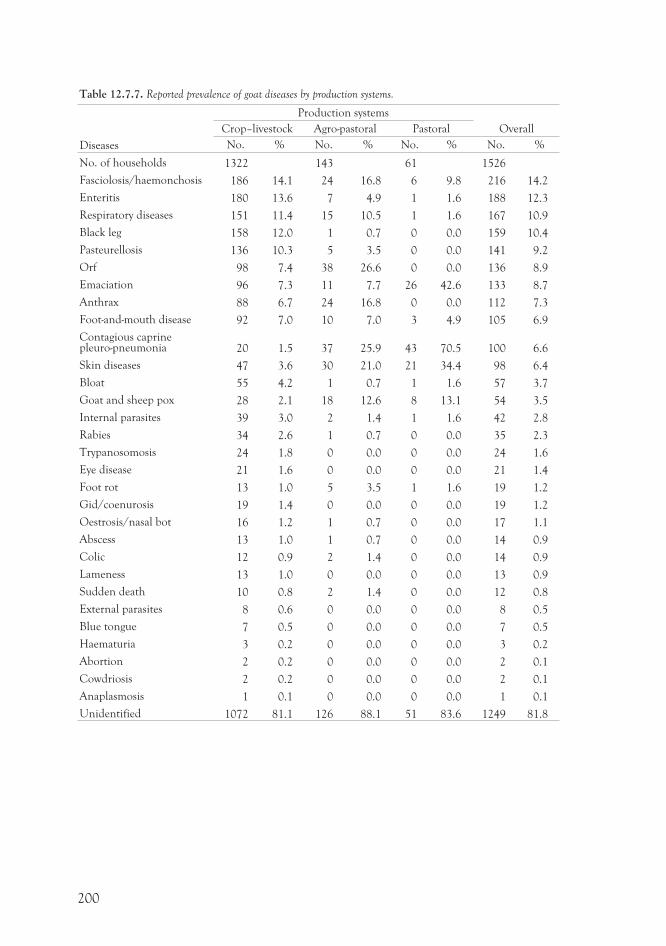
Table 12.7.7. Reported prevalence of goat diseases by production systems.
Diseases
Production systems
OverallCrop–livestock Agro-pastoral Pastoral
No. % No. % No. % No. %
No. of households 1322 143 61 1526
Fasciolosis/haemonchosis 186 14.1 24 16.8 6 9.8 216 14.2
Enteritis 180 13.6 7 4.9 1 1.6 188 12.3
Respiratory diseases 151 11.4 15 10.5 1 1.6 167 10.9
Black leg 158 12.0 1 0.7 0 0.0 159 10.4
Pasteurellosis 136 10.3 5 3.5 0 0.0 141 9.2
Orf 98 7.4 38 26.6 0 0.0 136 8.9
Emaciation 96 7.3 11 7.7 26 42.6 133 8.7
Anthrax 88 6.7 24 16.8 0 0.0 112 7.3
Foot-and-mouth disease 92 7.0 10 7.0 3 4.9 105 6.9
Contagious caprinepleuro-pneumonia 20 1.5 37 25.9 43 70.5 100 6.6
Skin diseases 47 3.6 30 21.0 21 34.4 98 6.4
Bloat 55 4.2 1 0.7 1 1.6 57 3.7
Goat and sheep pox 28 2.1 18 12.6 8 13.1 54 3.5
Internal parasites 39 3.0 2 1.4 1 1.6 42 2.8
Rabies 34 2.6 1 0.7 0 0.0 35 2.3
Trypanosomosis 24 1.8 0 0.0 0 0.0 24 1.6
Eye disease 21 1.6 0 0.0 0 0.0 21 1.4
Foot rot 13 1.0 5 3.5 1 1.6 19 1.2
Gid/coenurosis 19 1.4 0 0.0 0 0.0 19 1.2
Oestrosis/nasal bot 16 1.2 1 0.7 0 0.0 17 1.1
Abscess 13 1.0 1 0.7 0 0.0 14 0.9
Colic 12 0.9 2 1.4 0 0.0 14 0.9
Lameness 13 1.0 0 0.0 0 0.0 13 0.9
Sudden death 10 0.8 2 1.4 0 0.0 12 0.8
External parasites 8 0.6 0 0.0 0 0.0 8 0.5
Blue tongue 7 0.5 0 0.0 0 0.0 7 0.5
Haematuria 3 0.2 0 0.0 0 0.0 3 0.2
Abortion 2 0.2 0 0.0 0 0.0 2 0.1
Cowdriosis 2 0.2 0 0.0 0 0.0 2 0.1
Anaplasmosis 1 0.1 0 0.0 0 0.0 1 0.1
Unidentified 1072 81.1 126 88.1 51 83.6 1249 81.8
200
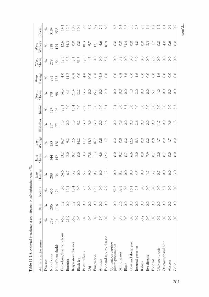
201
Tab
le12.7
.8.
Rep
orte
dpr
evale
nce
ofgo
at
dise
ase
sby
adm
inis
trati
vezo
nes
(%).
Ad
min
istr
ativ
ezo
nes
Ars
iB
ale
Bo
ran
aE
ast
Har
arge
Eas
tS
hew
aE
ast
Wel
lega
Illu
bab
or
Jim
ma
No
rth
Sh
ewa
Wes
tH
arar
geW
est
Sh
ewa
Wes
tW
elle
gaO
vera
ll
Dis
ease
s%
%%
%%
%%
%%
%%
%%
No
.o
fca
ses
219
206
456
288
344
253
117
174
178
292
279
378
3184
No
.o
fh
ou
seh
old
s114
116
174
134
152
120
77
96
98
125
154
175
1535
Fas
cio
losi
s/h
aem
on
cho
sis
46.5
1.7
0.6
24.6
13.2
16.7
1.3
28.1
14.3
4.0
12.3
12.6
14.1
En
teri
tis
21.9
0.9
12.1
6.7
2.0
9.2
0.0
0.0
4.1
11.2
3.2
54.3
12.2
Res
pir
ato
ryd
isea
ses
36.8
1.7
18.4
3.7
9.2
2.5
1.3
10.4
21.4
20.8
7.1
0.0
10.9
Bla
ckle
g0.0
0.0
0.0
0.0
0.0
54.2
5.2
0.0
12.2
0.0
51.3
0.0
10.4
Pas
teu
rell
osi
s0.0
0.0
2.3
5.2
3.3
11.7
13.0
25.0
13.3
4.8
17.5
18.3
9.3
Orf
0.0
0.0
0.0
9.0
17.8
13.3
3.9
4.2
0.0
40.0
4.5
9.7
8.9
Em
acia
tio
n0.0
0.0
19.5
0.7
1.3
16.7
13.0
0.0
35.7
0.8
0.0
17.1
8.7
An
thra
x7.0
0.0
0.0
6.0
4.6
0.8
0.0
0.0
0.0
64.8
0.0
4.6
7.4
Fo
ot-an
d-m
ou
thd
isea
se0.0
0.0
2.9
11.2
32.2
1.7
2.6
3.1
2.0
0.0
5.2
10.9
6.8
Co
nta
gio
us
cap
rin
ep
leu
ro-p
neu
mo
nia
0.0
0.0
52.3
0.0
0.0
0.0
0.0
9.4
0.0
0.0
0.0
0.0
6.5
Skin
dis
ease
s0.9
2.6
32.2
8.2
9.2
0.8
7.8
0.0
0.0
0.8
3.2
0.0
6.4
Blo
at0.0
0.0
0.6
0.0
0.7
0.0
0.0
8.3
0.0
5.6
0.0
23.4
3.8
Go
atan
dsh
eep
po
x0.0
0.0
16.1
0.0
6.6
12.5
0.0
0.0
1.0
0.0
0.0
0.0
3.5
Inte
rnal
par
asit
es0.9
0.0
2.3
4.5
2.0
8.3
2.6
0.0
2.0
1.6
3.9
4.0
2.8
Rab
ies
30.7
0.0
0.0
0.0
0.0
0.0
0.0
0.0
0.0
0.0
0.0
0.0
2.3
Eye
dis
ease
0.0
0.0
0.0
3.7
7.9
0.0
0.0
0.0
0.0
0.0
0.0
2.3
1.4
Fo
ot
rot
0.0
0.0
0.0
3.7
0.7
0.8
0.0
0.0
5.1
0.0
2.6
1.7
1.2
Gid
/co
enu
rosi
s0.9
0.0
0.0
0.7
2.0
1.7
11.7
0.0
1.0
1.6
0.0
0.0
1.2
Oes
tro
sis/
nas
alb
lot
0.0
0.0
5.2
0.0
0.7
0.0
0.0
0.0
0.0
0.0
0.0
4.0
1.1
Ab
sces
s0.0
0.0
0.0
6.0
0.0
1.7
3.9
0.0
0.0
0.0
0.0
0.6
0.9
Co
lic
0.0
0.0
0.0
3.0
0.0
0.0
1.3
8.3
0.0
0.0
0.6
0.0
0.9
con
t’d
...
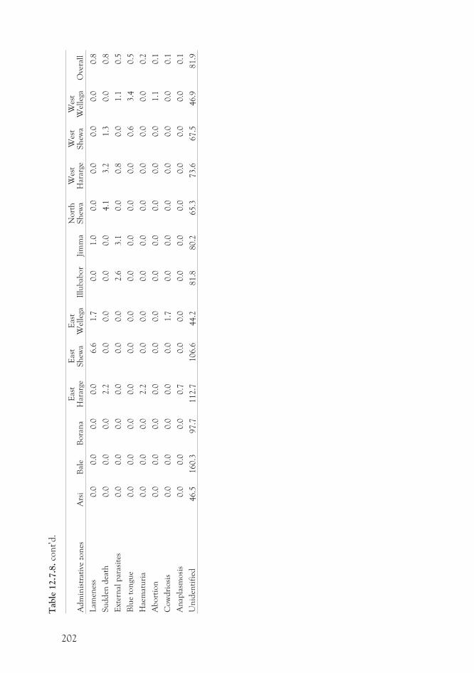
202
Ad
min
istr
ativ
ezo
nes
Ars
iB
ale
Bo
ran
aE
ast
Har
arge
Eas
tS
hew
aE
ast
Wel
lega
Illu
bab
or
Jim
ma
No
rth
Sh
ewa
Wes
tH
arar
geW
est
Sh
ewa
Wes
tW
elle
gaO
vera
ll
Lam
enes
s0.0
0.0
0.0
0.0
6.6
1.7
0.0
1.0
0.0
0.0
0.0
0.0
0.8
Su
dd
end
eath
0.0
0.0
0.0
2.2
0.0
0.0
0.0
0.0
4.1
3.2
1.3
0.0
0.8
Ext
ern
alp
aras
ites
0.0
0.0
0.0
0.0
0.0
0.0
2.6
3.1
0.0
0.8
0.0
1.1
0.5
Blu
eto
ngu
e0.0
0.0
0.0
0.0
0.0
0.0
0.0
0.0
0.0
0.0
0.6
3.4
0.5
Hae
mat
uri
a0.0
0.0
0.0
2.2
0.0
0.0
0.0
0.0
0.0
0.0
0.0
0.0
0.2
Ab
ort
ion
0.0
0.0
0.0
0.0
0.0
0.0
0.0
0.0
0.0
0.0
0.0
1.1
0.1
Co
wd
rio
sis
0.0
0.0
0.0
0.0
0.0
1.7
0.0
0.0
0.0
0.0
0.0
0.0
0.1
An
apla
smo
sis
0.0
0.0
0.0
0.7
0.0
0.0
0.0
0.0
0.0
0.0
0.0
0.0
0.1
Un
iden
tifi
ed46.5
160.3
97.7
112.7
106.6
44.2
81.8
80.2
65.3
73.6
67.5
46.9
81.9
Tab
le12.7
.8.
con
t’d
.
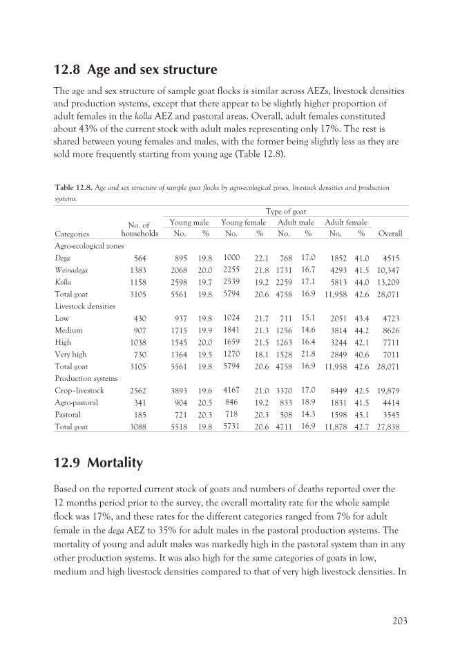
12.8 Age and sex structureThe age and sex structure of sample goat flocks is similar across AEZs, livestock densities
and production systems, except that there appear to be slightly higher proportion of
adult females in the kolla AEZ and pastoral areas. Overall, adult females constituted
about 43% of the current stock with adult males representing only 17%. The rest is
shared between young females and males, with the former being slightly less as they are
sold more frequently starting from young age (Table 12.8).
Table 12.8. Age and sex structure of sample goat flocks by agro-ecological zones, livestock densities and production
systems.
CategoriesNo. of
households
Type of goat
Young male Young female Adult male Adult female
OverallNo. % No. % No. % No. %
Agro-ecological zones
Dega 564 895 19.8 1000 22.1 768 17.0 1852 41.0 4515
Weinadega 1383 2068 20.0 2255 21.8 1731 16.7 4293 41.5 10,347
Kolla 1158 2598 19.7 2539 19.2 2259 17.1 5813 44.0 13,209
Total goat 3105 5561 19.8 5794 20.6 4758 16.9 11,958 42.6 28,071
Livestock densities
Low 430 937 19.8 1024 21.7 711 15.1 2051 43.4 4723
Medium 907 1715 19.9 1841 21.3 1256 14.6 3814 44.2 8626
High 1038 1545 20.0 1659 21.5 1263 16.4 3244 42.1 7711
Very high 730 1364 19.5 1270 18.1 1528 21.8 2849 40.6 7011
Total goat 3105 5561 19.8 5794 20.6 4758 16.9 11,958 42.6 28,071
Production systems
Crop–livestock 2562 3893 19.6 4167 21.0 3370 17.0 8449 42.5 19,879
Agro-pastoral 341 904 20.5 846 19.2 833 18.9 1831 41.5 4414
Pastoral 185 721 20.3 718 20.3 508 14.3 1598 45.1 3545
Total goat 3088 5518 19.8 5731 20.6 4711 16.9 11,878 42.7 27,838
12.9 Mortality
Based on the reported current stock of goats and numbers of deaths reported over the
12 months period prior to the survey, the overall mortality rate for the whole sample
flock was 17%, and these rates for the different categories ranged from 7% for adult
female in the dega AEZ to 35% for adult males in the pastoral production systems. The
mortality of young and adult males was markedly high in the pastoral system than in any
other production systems. It was also high for the same categories of goats in low,
medium and high livestock densities compared to that of very high livestock densities. In
203
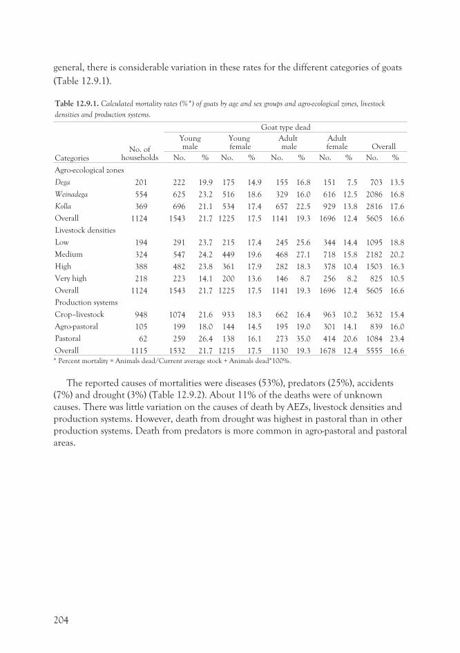
general, there is considerable variation in these rates for the different categories of goats
(Table 12.9.1).
Table 12.9.1. Calculated mortality rates (%*) of goats by age and sex groups and agro-ecological zones, livestock
densities and production systems.
CategoriesNo. of
households
Goat type dead
Youngmale
Youngfemale
Adultmale
Adultfemale Overall
No. % No. % No. % No. % No. %
Agro-ecological zones
Dega 201 222 19.9 175 14.9 155 16.8 151 7.5 703 13.5
Weinadega 554 625 23.2 516 18.6 329 16.0 616 12.5 2086 16.8
Kolla 369 696 21.1 534 17.4 657 22.5 929 13.8 2816 17.6
Overall 1124 1543 21.7 1225 17.5 1141 19.3 1696 12.4 5605 16.6
Livestock densities
Low 194 291 23.7 215 17.4 245 25.6 344 14.4 1095 18.8
Medium 324 547 24.2 449 19.6 468 27.1 718 15.8 2182 20.2
High 388 482 23.8 361 17.9 282 18.3 378 10.4 1503 16.3
Very high 218 223 14.1 200 13.6 146 8.7 256 8.2 825 10.5
Overall 1124 1543 21.7 1225 17.5 1141 19.3 1696 12.4 5605 16.6
Production systems
Crop–livestock 948 1074 21.6 933 18.3 662 16.4 963 10.2 3632 15.4
Agro-pastoral 105 199 18.0 144 14.5 195 19.0 301 14.1 839 16.0
Pastoral 62 259 26.4 138 16.1 273 35.0 414 20.6 1084 23.4
Overall 1115 1532 21.7 1215 17.5 1130 19.3 1678 12.4 5555 16.6
* Percent mortality = Animals dead/Current average stock + Animals dead*100%.
The reported causes of mortalities were diseases (53%), predators (25%), accidents
(7%) and drought (3%) (Table 12.9.2). About 11% of the deaths were of unknown
causes. There was little variation on the causes of death by AEZs, livestock densities and
production systems. However, death from drought was highest in pastoral than in other
production systems. Death from predators is more common in agro-pastoral and pastoral
areas.
204
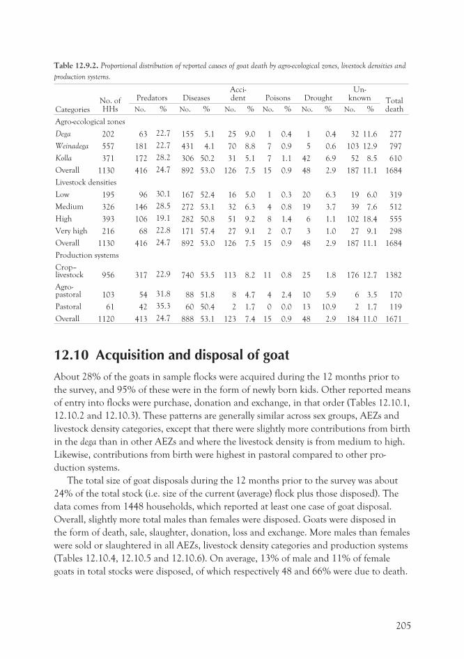
Table 12.9.2. Proportional distribution of reported causes of goat death by agro-ecological zones, livestock densities and
production systems.
CategoriesNo. ofHHs
Predators DiseasesAcci-dent Poisons Drought
Un-known Total
deathNo. % No. % No. % No. % No. % No. %
Agro-ecological zones
Dega 202 63 22.7 155 5.1 25 9.0 1 0.4 1 0.4 32 11.6 277
Weinadega 557 181 22.7 431 4.1 70 8.8 7 0.9 5 0.6 103 12.9 797
Kolla 371 172 28.2 306 50.2 31 5.1 7 1.1 42 6.9 52 8.5 610
Overall 1130 416 24.7 892 53.0 126 7.5 15 0.9 48 2.9 187 11.1 1684
Livestock densities
Low 195 96 30.1 167 52.4 16 5.0 1 0.3 20 6.3 19 6.0 319
Medium 326 146 28.5 272 53.1 32 6.3 4 0.8 19 3.7 39 7.6 512
High 393 106 19.1 282 50.8 51 9.2 8 1.4 6 1.1 102 18.4 555
Very high 216 68 22.8 171 57.4 27 9.1 2 0.7 3 1.0 27 9.1 298
Overall 1130 416 24.7 892 53.0 126 7.5 15 0.9 48 2.9 187 11.1 1684
Production systems
Crop–livestock 956 317 22.9 740 53.5 113 8.2 11 0.8 25 1.8 176 12.7 1382
Agro-pastoral 103 54 31.8 88 51.8 8 4.7 4 2.4 10 5.9 6 3.5 170
Pastoral 61 42 35.3 60 50.4 2 1.7 0 0.0 13 10.9 2 1.7 119
Overall 1120 413 24.7 888 53.1 123 7.4 15 0.9 48 2.9 184 11.0 1671
12.10 Acquisition and disposal of goatAbout 28% of the goats in sample flocks were acquired during the 12 months prior to
the survey, and 95% of these were in the form of newly born kids. Other reported means
of entry into flocks were purchase, donation and exchange, in that order (Tables 12.10.1,
12.10.2 and 12.10.3). These patterns are generally similar across sex groups, AEZs and
livestock density categories, except that there were slightly more contributions from birth
in the dega than in other AEZs and where the livestock density is from medium to high.
Likewise, contributions from birth were highest in pastoral compared to other pro-
duction systems.
The total size of goat disposals during the 12 months prior to the survey was about
24% of the total stock (i.e. size of the current (average) flock plus those disposed). The
data comes from 1448 households, which reported at least one case of goat disposal.
Overall, slightly more total males than females were disposed. Goats were disposed in
the form of death, sale, slaughter, donation, loss and exchange. More males than females
were sold or slaughtered in all AEZs, livestock density categories and production systems
(Tables 12.10.4, 12.10.5 and 12.10.6). On average, 13% of male and 11% of female
goats in total stocks were disposed, of which respectively 48 and 66% were due to death.
205
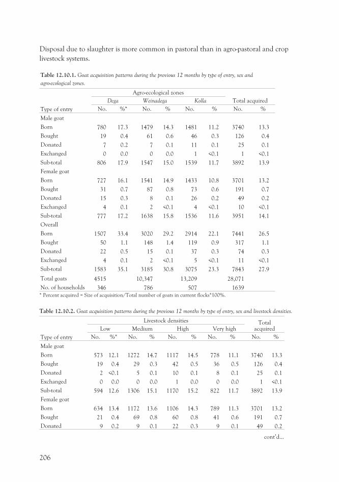
Disposal due to slaughter is more common in pastoral than in agro-pastoral and crop
livestock systems.
Table 12.10.1. Goat acquisition patterns during the previous 12 months by type of entry, sex and
agro-ecological zones.
Type of entry
Agro-ecological zones
Total acquiredDega Weinadega Kolla
No. %* No. % No. % No. %
Male goat
Born 780 17.3 1479 14.3 1481 11.2 3740 13.3
Bought 19 0.4 61 0.6 46 0.3 126 0.4
Donated 7 0.2 7 0.1 11 0.1 25 0.1
Exchanged 0 0.0 0 0.0 1 <0.1 1 <0.1
Sub-total 806 17.9 1547 15.0 1539 11.7 3892 13.9
Female goat
Born 727 16.1 1541 14.9 1433 10.8 3701 13.2
Bought 31 0.7 87 0.8 73 0.6 191 0.7
Donated 15 0.3 8 0.1 26 0.2 49 0.2
Exchanged 4 0.1 2 <0.1 4 <0.1 10 <0.1
Sub-total 777 17.2 1638 15.8 1536 11.6 3951 14.1
Overall
Born 1507 33.4 3020 29.2 2914 22.1 7441 26.5
Bought 50 1.1 148 1.4 119 0.9 317 1.1
Donated 22 0.5 15 0.1 37 0.3 74 0.3
Exchanged 4 0.1 2 <0.1 5 <0.1 11 <0.1
Sub-total 1583 35.1 3185 30.8 3075 23.3 7843 27.9
Total goats 4515 10,347 13,209 28,071
No. of households 346 786 507 1639
* Percent acquired = Size of acquisition/Total number of goats in current flocks*100%.
Table 12.10.2. Goat acquisition patterns during the previous 12 months by type of entry, sex and livestock densities.
Type of entry
Livestock densities TotalacquiredLow Medium High Very high
No. %* No. % No. % No. % No. %
Male goat
Born 573 12.1 1272 14.7 1117 14.5 778 11.1 3740 13.3
Bought 19 0.4 29 0.3 42 0.5 36 0.5 126 0.4
Donated 2 <0.1 5 0.1 10 0.1 8 0.1 25 0.1
Exchanged 0 0.0 0 0.0 1 0.0 0 0.0 1 <0.1
Sub-total 594 12.6 1306 15.1 1170 15.2 822 11.7 3892 13.9
Female goat
Born 634 13.4 1172 13.6 1106 14.3 789 11.3 3701 13.2
Bought 21 0.4 69 0.8 60 0.8 41 0.6 191 0.7
Donated 9 0.2 9 0.1 22 0.3 9 0.1 49 0.2
206
cont’d...
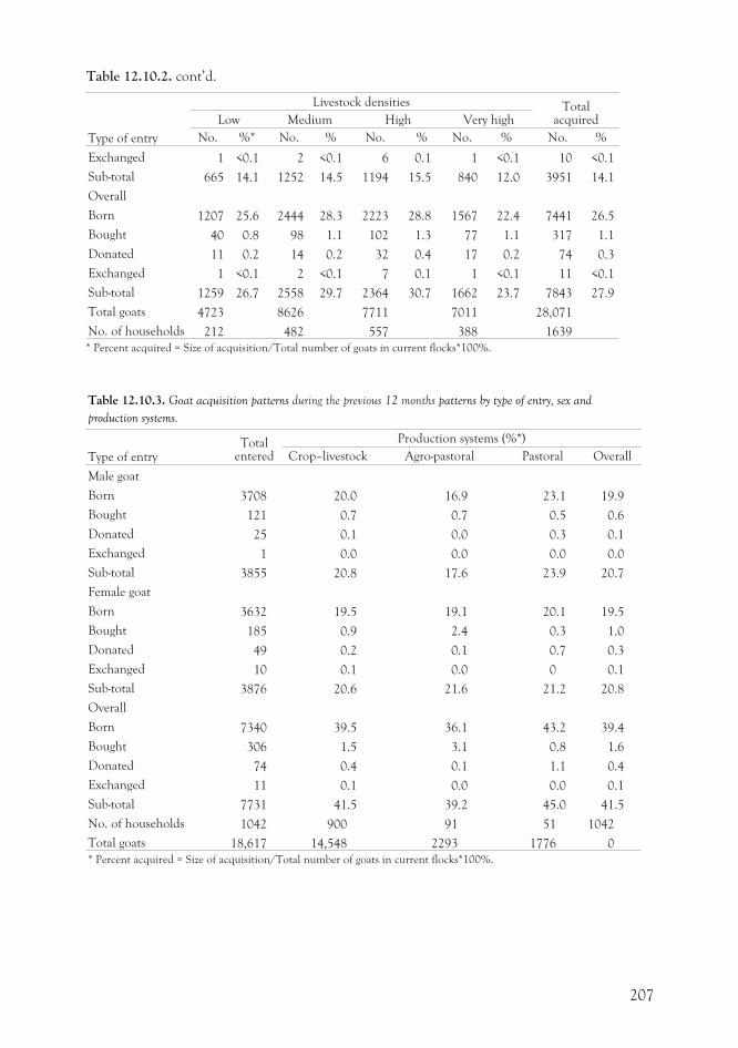
Type of entry
Livestock densities TotalacquiredLow Medium High Very high
No. %* No. % No. % No. % No. %
Exchanged 1 <0.1 2 <0.1 6 0.1 1 <0.1 10 <0.1
Sub-total 665 14.1 1252 14.5 1194 15.5 840 12.0 3951 14.1
Overall
Born 1207 25.6 2444 28.3 2223 28.8 1567 22.4 7441 26.5
Bought 40 0.8 98 1.1 102 1.3 77 1.1 317 1.1
Donated 11 0.2 14 0.2 32 0.4 17 0.2 74 0.3
Exchanged 1 <0.1 2 <0.1 7 0.1 1 <0.1 11 <0.1
Sub-total 1259 26.7 2558 29.7 2364 30.7 1662 23.7 7843 27.9
Total goats 4723 8626 7711 7011 28,071
No. of households 212 482 557 388 1639
* Percent acquired = Size of acquisition/Total number of goats in current flocks*100%.
Table 12.10.3. Goat acquisition patterns during the previous 12 months patterns by type of entry, sex and
production systems.
Type of entryTotal
entered
Production systems (%*)
Crop–livestock Agro-pastoral Pastoral Overall
Male goat
Born 3708 20.0 16.9 23.1 19.9
Bought 121 0.7 0.7 0.5 0.6
Donated 25 0.1 0.0 0.3 0.1
Exchanged 1 0.0 0.0 0.0 0.0
Sub-total 3855 20.8 17.6 23.9 20.7
Female goat
Born 3632 19.5 19.1 20.1 19.5
Bought 185 0.9 2.4 0.3 1.0
Donated 49 0.2 0.1 0.7 0.3
Exchanged 10 0.1 0.0 0 0.1
Sub-total 3876 20.6 21.6 21.2 20.8
Overall
Born 7340 39.5 36.1 43.2 39.4
Bought 306 1.5 3.1 0.8 1.6
Donated 74 0.4 0.1 1.1 0.4
Exchanged 11 0.1 0.0 0.0 0.1
Sub-total 7731 41.5 39.2 45.0 41.5
No. of households 1042 900 91 51 1042
Total goats 18,617 14,548 2293 1776 0
* Percent acquired = Size of acquisition/Total number of goats in current flocks*100%.
207
Table 12.10.2. cont’d.
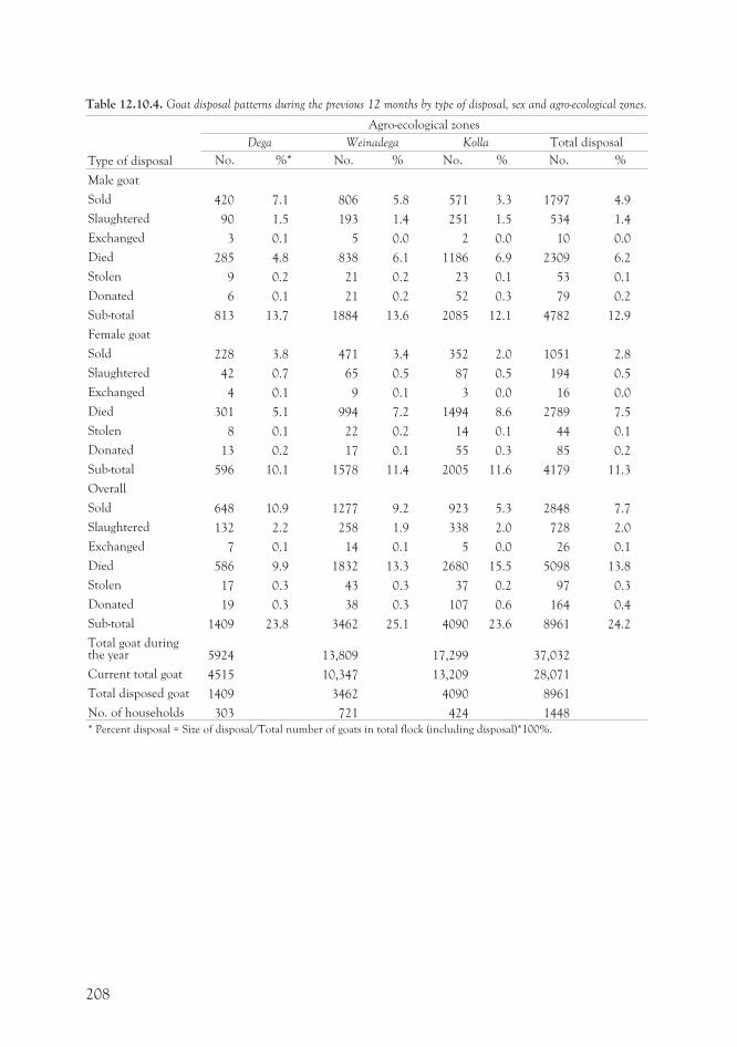
Table 12.10.4. Goat disposal patterns during the previous 12 months by type of disposal, sex and agro-ecological zones.
Type of disposal
Agro-ecological zones
Dega Weinadega Kolla Total disposal
No. %* No. % No. % No. %
Male goat
Sold 420 7.1 806 5.8 571 3.3 1797 4.9
Slaughtered 90 1.5 193 1.4 251 1.5 534 1.4
Exchanged 3 0.1 5 0.0 2 0.0 10 0.0
Died 285 4.8 838 6.1 1186 6.9 2309 6.2
Stolen 9 0.2 21 0.2 23 0.1 53 0.1
Donated 6 0.1 21 0.2 52 0.3 79 0.2
Sub-total 813 13.7 1884 13.6 2085 12.1 4782 12.9
Female goat
Sold 228 3.8 471 3.4 352 2.0 1051 2.8
Slaughtered 42 0.7 65 0.5 87 0.5 194 0.5
Exchanged 4 0.1 9 0.1 3 0.0 16 0.0
Died 301 5.1 994 7.2 1494 8.6 2789 7.5
Stolen 8 0.1 22 0.2 14 0.1 44 0.1
Donated 13 0.2 17 0.1 55 0.3 85 0.2
Sub-total 596 10.1 1578 11.4 2005 11.6 4179 11.3
Overall
Sold 648 10.9 1277 9.2 923 5.3 2848 7.7
Slaughtered 132 2.2 258 1.9 338 2.0 728 2.0
Exchanged 7 0.1 14 0.1 5 0.0 26 0.1
Died 586 9.9 1832 13.3 2680 15.5 5098 13.8
Stolen 17 0.3 43 0.3 37 0.2 97 0.3
Donated 19 0.3 38 0.3 107 0.6 164 0.4
Sub-total 1409 23.8 3462 25.1 4090 23.6 8961 24.2
Total goat duringthe year 5924 13,809 17,299 37,032
Current total goat 4515 10,347 13,209 28,071
Total disposed goat 1409 3462 4090 8961
No. of households 303 721 424 1448
* Percent disposal = Size of disposal/Total number of goats in total flock (including disposal)*100%.
208
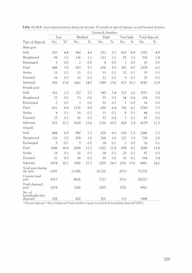
Table 12.10.5. Goat disposal patterns during the previous 12 months by type of disposal, sex and livestock densities.
Type of disposal
Livestock densities
Low Medium High Very high Total disposal
No. %* No. % No. % No. % No. %
Male goat
Sold 283 4.4 568 4.8 531 5.2 415 4.9 1797 4.9
Slaughtered 94 1.5 136 1.1 211 2.1 93 1.1 534 1.4
Exchanged 3 0.0 2 0.0 4 0.0 1 0.0 10 0.0
Died 448 7.0 912 7.7 606 5.9 343 4.0 2309 6.2
Stolen 15 0.2 11 0.1 15 0.1 12 0.1 53 0.1
Donated 16 0.3 32 0.3 22 0.2 9 0.1 79 0.2
Sub-total 859 13.4 1661 14.0 1389 13.6 873 10.3 4782 12.9
Female goat
Sold 161 2.5 322 2.7 345 3.4 223 2.6 1051 2.8
Slaughtered 32 0.5 73 0.6 55 0.5 34 0.4 194 0.5
Exchanged 2 0.0 3 0.0 10 0.1 1 0.0 16 0.0
Died 601 9.4 1176 9.9 656 6.4 356 4.2 2789 7.5
Stolen 4 0.1 19 0.2 13 0.1 8 0.1 44 0.1
Donated 15 0.2 26 0.2 37 0.4 7 0.1 85 0.2
Sub-total 815 12.7 1619 13.6 1116 10.9 629 7.4 4179 11.3
Overall
Sold 444 6.9 890 7.5 876 8.6 638 7.5 2848 7.7
Slaughtered 126 2.0 209 1.8 266 2.6 127 1.5 728 2.0
Exchanged 5 0.1 5 0.0 14 0.1 2 0.0 26 0.1
Died 1049 16.4 2088 17.5 1262 12.4 699 8.2 5098 13.8
Stolen 19 0.3 30 0.3 28 0.3 20 0.2 97 0.3
Donated 31 0.5 58 0.5 59 0.6 16 0.2 164 0.4
Sub-total 1674 26.2 3280 27.5 2505 24.5 1502 17.6 8961 24.2
Total goat duringthe year 6397 11,906 10,216 8513 37,032
Current totalgoat 4723 8626 7711 7011 28,071
Total disposedgoat 1674 3280 2505 1502 8961
No. ofhouseholds whodisposed 208 420 507 313 1448
* Percent disposal = Size of disposal/Total number of goats in total flock (including disposal)*100%.
209
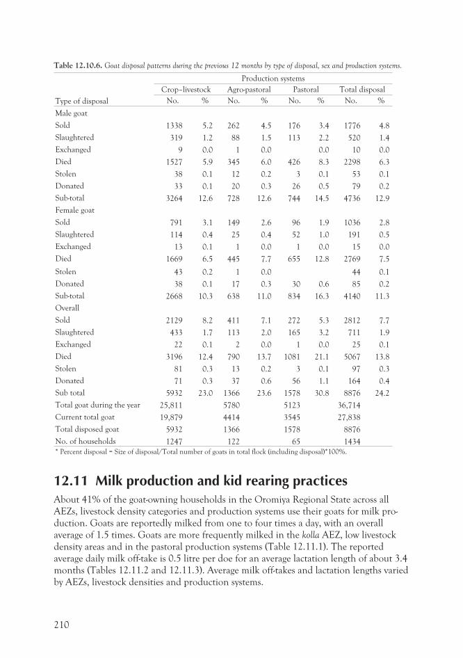
Table 12.10.6. Goat disposal patterns during the previous 12 months by type of disposal, sex and production systems.
Type of disposal
Production systems
Crop–livestock Agro-pastoral Pastoral Total disposal
No. % No. % No. % No. %
Male goat
Sold 1338 5.2 262 4.5 176 3.4 1776 4.8
Slaughtered 319 1.2 88 1.5 113 2.2 520 1.4
Exchanged 9 0.0 1 0.0 0.0 10 0.0
Died 1527 5.9 345 6.0 426 8.3 2298 6.3
Stolen 38 0.1 12 0.2 3 0.1 53 0.1
Donated 33 0.1 20 0.3 26 0.5 79 0.2
Sub-total 3264 12.6 728 12.6 744 14.5 4736 12.9
Female goat
Sold 791 3.1 149 2.6 96 1.9 1036 2.8
Slaughtered 114 0.4 25 0.4 52 1.0 191 0.5
Exchanged 13 0.1 1 0.0 1 0.0 15 0.0
Died 1669 6.5 445 7.7 655 12.8 2769 7.5
Stolen 43 0.2 1 0.0 44 0.1
Donated 38 0.1 17 0.3 30 0.6 85 0.2
Sub-total 2668 10.3 638 11.0 834 16.3 4140 11.3
Overall
Sold 2129 8.2 411 7.1 272 5.3 2812 7.7
Slaughtered 433 1.7 113 2.0 165 3.2 711 1.9
Exchanged 22 0.1 2 0.0 1 0.0 25 0.1
Died 3196 12.4 790 13.7 1081 21.1 5067 13.8
Stolen 81 0.3 13 0.2 3 0.1 97 0.3
Donated 71 0.3 37 0.6 56 1.1 164 0.4
Sub total 5932 23.0 1366 23.6 1578 30.8 8876 24.2
Total goat during the year 25,811 5780 5123 36,714
Current total goat 19,879 4414 3545 27,838
Total disposed goat 5932 1366 1578 8876
No. of households 1247 122 65 1434
* Percent disposal = Size of disposal/Total number of goats in total flock (including disposal)*100%.
12.11 Milk production and kid rearing practicesAbout 41% of the goat-owning households in the Oromiya Regional State across all
AEZs, livestock density categories and production systems use their goats for milk pro-
duction. Goats are reportedly milked from one to four times a day, with an overall
average of 1.5 times. Goats are more frequently milked in the kolla AEZ, low livestock
density areas and in the pastoral production systems (Table 12.11.1). The reported
average daily milk off-take is 0.5 litre per doe for an average lactation length of about 3.4
months (Tables 12.11.2 and 12.11.3). Average milk off-takes and lactation lengths varied
by AEZs, livestock densities and production systems.
210
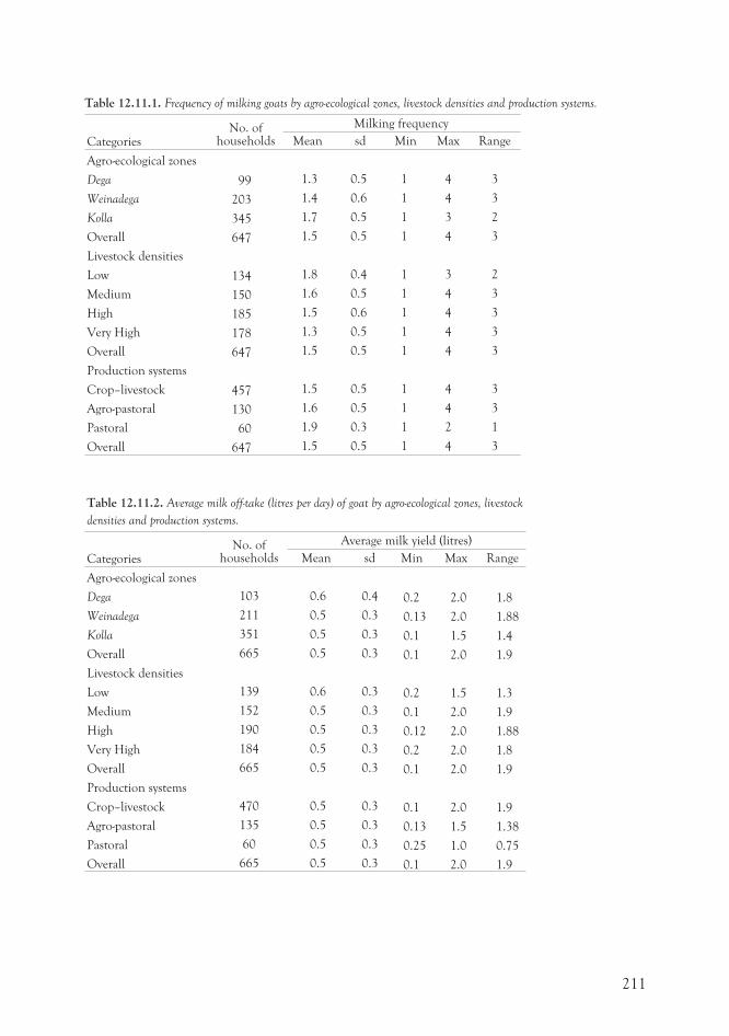
Table 12.11.1. Frequency of milking goats by agro-ecological zones, livestock densities and production systems.
CategoriesNo. of
households
Milking frequency
Mean sd Min Max Range
Agro-ecological zones
Dega 99 1.3 0.5 1 4 3
Weinadega 203 1.4 0.6 1 4 3
Kolla 345 1.7 0.5 1 3 2
Overall 647 1.5 0.5 1 4 3
Livestock densities
Low 134 1.8 0.4 1 3 2
Medium 150 1.6 0.5 1 4 3
High 185 1.5 0.6 1 4 3
Very High 178 1.3 0.5 1 4 3
Overall 647 1.5 0.5 1 4 3
Production systems
Crop–livestock 457 1.5 0.5 1 4 3
Agro-pastoral 130 1.6 0.5 1 4 3
Pastoral 60 1.9 0.3 1 2 1
Overall 647 1.5 0.5 1 4 3
Table 12.11.2. Average milk off-take (litres per day) of goat by agro-ecological zones, livestock
densities and production systems.
CategoriesNo. of
households
Average milk yield (litres)
Mean sd Min Max Range
Agro-ecological zones
Dega 103 0.6 0.4 0.2 2.0 1.8
Weinadega 211 0.5 0.3 0.13 2.0 1.88
Kolla 351 0.5 0.3 0.1 1.5 1.4
Overall 665 0.5 0.3 0.1 2.0 1.9
Livestock densities
Low 139 0.6 0.3 0.2 1.5 1.3
Medium 152 0.5 0.3 0.1 2.0 1.9
High 190 0.5 0.3 0.12 2.0 1.88
Very High 184 0.5 0.3 0.2 2.0 1.8
Overall 665 0.5 0.3 0.1 2.0 1.9
Production systems
Crop–livestock 470 0.5 0.3 0.1 2.0 1.9
Agro-pastoral 135 0.5 0.3 0.13 1.5 1.38
Pastoral 60 0.5 0.3 0.25 1.0 0.75
Overall 665 0.5 0.3 0.1 2.0 1.9
211
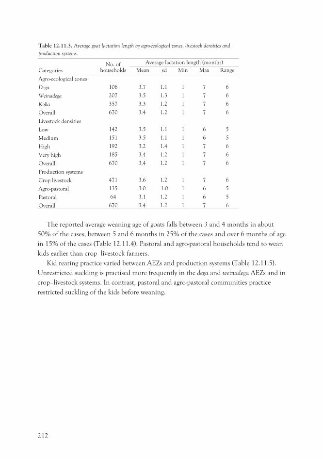
Table 12.11.3. Average goat lactation length by agro-ecological zones, livestock densities and
production systems.
CategoriesNo. of
households
Average lactation length (months)
Mean sd Min Max Range
Agro-ecological zones
Dega 106 3.7 1.1 1 7 6
Weinadega 207 3.5 1.3 1 7 6
Kolla 357 3.3 1.2 1 7 6
Overall 670 3.4 1.2 1 7 6
Livestock densities
Low 142 3.5 1.1 1 6 5
Medium 151 3.5 1.1 1 6 5
High 192 3.2 1.4 1 7 6
Very high 185 3.4 1.2 1 7 6
Overall 670 3.4 1.2 1 7 6
Production systems
Crop livestock 471 3.6 1.2 1 7 6
Agro-pastoral 135 3.0 1.0 1 6 5
Pastoral 64 3.1 1.2 1 6 5
Overall 670 3.4 1.2 1 7 6
The reported average weaning age of goats falls between 3 and 4 months in about
50% of the cases, between 5 and 6 months in 25% of the cases and over 6 months of age
in 15% of the cases (Table 12.11.4). Pastoral and agro-pastoral households tend to wean
kids earlier than crop–livestock farmers.
Kid rearing practice varied between AEZs and production systems (Table 12.11.5).
Unrestricted suckling is practised more frequently in the dega and weinadega AEZs and in
crop–livestock systems. In contrast, pastoral and agro-pastoral communities practice
restricted suckling of the kids before weaning.
212
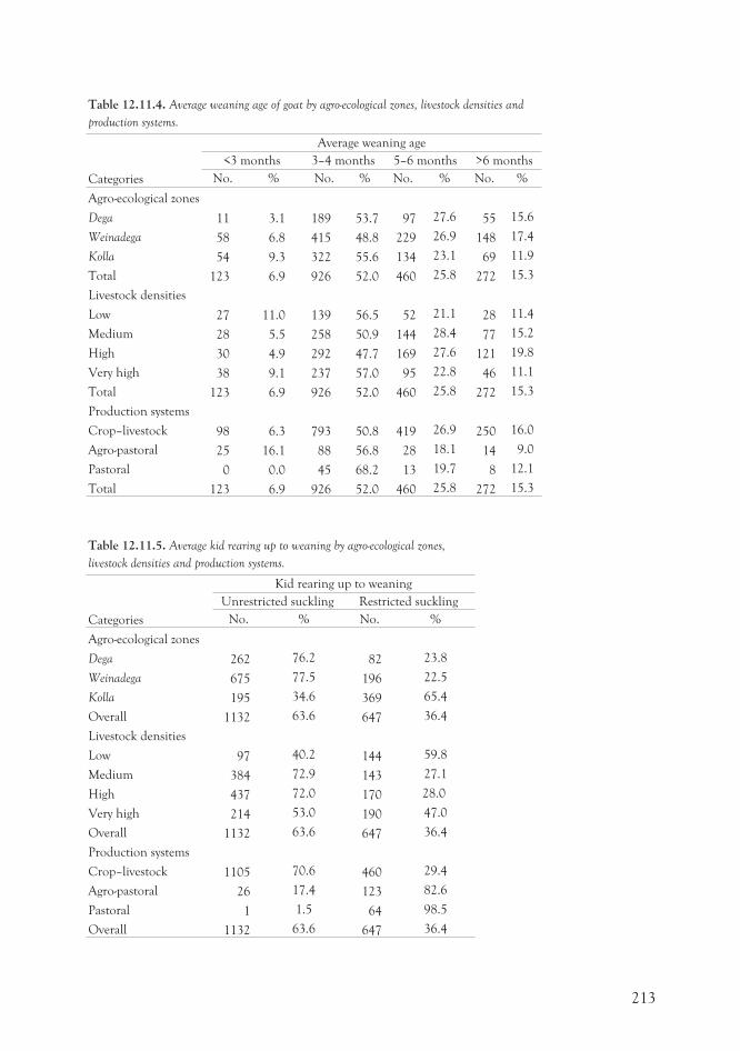
Table 12.11.4. Average weaning age of goat by agro-ecological zones, livestock densities and
production systems.
Categories
Average weaning age
<3 months 3–4 months 5–6 months >6 months
No. % No. % No. % No. %
Agro-ecological zones
Dega 11 3.1 189 53.7 97 27.6 55 15.6
Weinadega 58 6.8 415 48.8 229 26.9 148 17.4
Kolla 54 9.3 322 55.6 134 23.1 69 11.9
Total 123 6.9 926 52.0 460 25.8 272 15.3
Livestock densities
Low 27 11.0 139 56.5 52 21.1 28 11.4
Medium 28 5.5 258 50.9 144 28.4 77 15.2
High 30 4.9 292 47.7 169 27.6 121 19.8
Very high 38 9.1 237 57.0 95 22.8 46 11.1
Total 123 6.9 926 52.0 460 25.8 272 15.3
Production systems
Crop–livestock 98 6.3 793 50.8 419 26.9 250 16.0
Agro-pastoral 25 16.1 88 56.8 28 18.1 14 9.0
Pastoral 0 0.0 45 68.2 13 19.7 8 12.1
Total 123 6.9 926 52.0 460 25.8 272 15.3
Table 12.11.5. Average kid rearing up to weaning by agro-ecological zones,
livestock densities and production systems.
Categories
Kid rearing up to weaning
Unrestricted suckling Restricted suckling
No. % No. %
Agro-ecological zones
Dega 262 76.2 82 23.8
Weinadega 675 77.5 196 22.5
Kolla 195 34.6 369 65.4
Overall 1132 63.6 647 36.4
Livestock densities
Low 97 40.2 144 59.8
Medium 384 72.9 143 27.1
High 437 72.0 170 28.0
Very high 214 53.0 190 47.0
Overall 1132 63.6 647 36.4
Production systems
Crop–livestock 1105 70.6 460 29.4
Agro-pastoral 26 17.4 123 82.6
Pastoral 1 1.5 64 98.5
Overall 1132 63.6 647 36.4
213
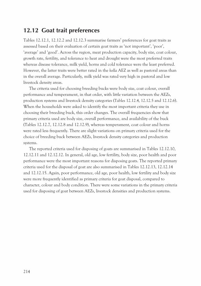
12.12 Goat trait preferences
Tables 12.12.1, 12.12.2 and 12.12.3 summarise farmers’ preferences for goat traits as
assessed based on their evaluation of certain goat traits as ‘not important’, ‘poor’,
‘average’ and ‘good’. Across the region, meat production capacity, body size, coat colour,
growth rate, fertility, and tolerance to heat and drought were the most preferred traits
whereas disease tolerance, milk yield, horns and cold tolerance were the least preferred.
However, the latter traits were better rated in the kolla AEZ as well as pastoral areas than
in the overall average. Particularly, milk yield was rated very high in pastoral and low
livestock density areas.
The criteria used for choosing breeding bucks were body size, coat colour, overall
performance and temperament, in that order, with little variation between the AEZs,
production systems and livestock density categories (Tables 12.12.4, 12.12.5 and 12.12.6).
When the households were asked to identify the most important criteria they use in
choosing their breeding buck, this order changes. The overall frequencies show that
primary criteria used are body size, overall performance, and availability of the buck
(Tables 12.12.7, 12.12.8 and 12.12.9), whereas temperament, coat colour and horns
were rated less frequently. There are slight variations on primary criteria used for the
choice of breeding buck between AEZs, livestock density categories and production
systems.
The reported criteria used for disposing of goats are summarised in Tables 12.12.10,
12.12.11 and 12.12.12. In general, old age, low fertility, body size, poor health and poor
performance were the most important reasons for disposing goats. The reported primary
criteria used for the disposal of goat are also summarised in Tables 12.12.13, 12.12.14
and 12.12.15. Again, poor performance, old age, poor health, low fertility and body size
were more frequently identified as primary criteria for goat disposal, compared to
character, colour and body condition. There were some variations in the primary criteria
used for disposing of goat between AEZs, livestock densities and production systems.
214
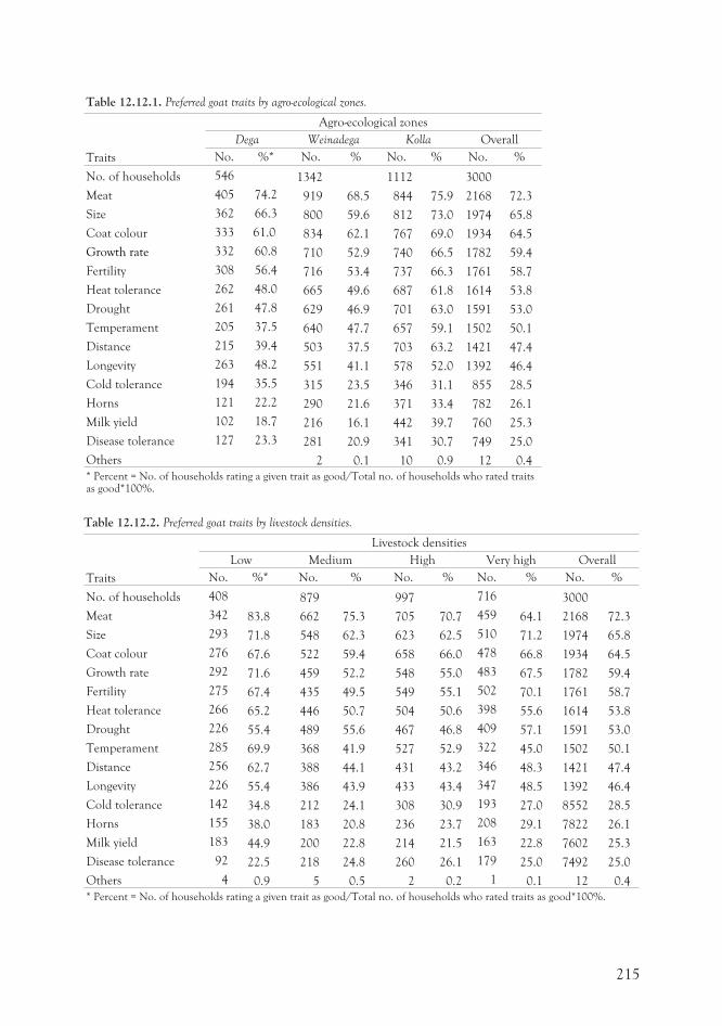
Table 12.12.1. Preferred goat traits by agro-ecological zones.
Traits
Agro-ecological zones
Dega Weinadega Kolla Overall
No. %* No. % No. % No. %
No. of households 546 1342 1112 3000
Meat 405 74.2 919 68.5 844 75.9 2168 72.3
Size 362 66.3 800 59.6 812 73.0 1974 65.8
Coat colour 333 61.0 834 62.1 767 69.0 1934 64.5
Growth rate 332 60.8 710 52.9 740 66.5 1782 59.4
Fertility 308 56.4 716 53.4 737 66.3 1761 58.7
Heat tolerance 262 48.0 665 49.6 687 61.8 1614 53.8
Drought 261 47.8 629 46.9 701 63.0 1591 53.0
Temperament 205 37.5 640 47.7 657 59.1 1502 50.1
Distance 215 39.4 503 37.5 703 63.2 1421 47.4
Longevity 263 48.2 551 41.1 578 52.0 1392 46.4
Cold tolerance 194 35.5 315 23.5 346 31.1 855 28.5
Horns 121 22.2 290 21.6 371 33.4 782 26.1
Milk yield 102 18.7 216 16.1 442 39.7 760 25.3
Disease tolerance 127 23.3 281 20.9 341 30.7 749 25.0
Others 2 0.1 10 0.9 12 0.4
* Percent = No. of households rating a given trait as good/Total no. of households who rated traitsas good*100%.
Table 12.12.2. Preferred goat traits by livestock densities.
Traits
Livestock densities
Low Medium High Very high Overall
No. %* No. % No. % No. % No. %
No. of households 408 879 997 716 3000
Meat 342 83.8 662 75.3 705 70.7 459 64.1 2168 72.3
Size 293 71.8 548 62.3 623 62.5 510 71.2 1974 65.8
Coat colour 276 67.6 522 59.4 658 66.0 478 66.8 1934 64.5
Growth rate 292 71.6 459 52.2 548 55.0 483 67.5 1782 59.4
Fertility 275 67.4 435 49.5 549 55.1 502 70.1 1761 58.7
Heat tolerance 266 65.2 446 50.7 504 50.6 398 55.6 1614 53.8
Drought 226 55.4 489 55.6 467 46.8 409 57.1 1591 53.0
Temperament 285 69.9 368 41.9 527 52.9 322 45.0 1502 50.1
Distance 256 62.7 388 44.1 431 43.2 346 48.3 1421 47.4
Longevity 226 55.4 386 43.9 433 43.4 347 48.5 1392 46.4
Cold tolerance 142 34.8 212 24.1 308 30.9 193 27.0 8552 28.5
Horns 155 38.0 183 20.8 236 23.7 208 29.1 7822 26.1
Milk yield 183 44.9 200 22.8 214 21.5 163 22.8 7602 25.3
Disease tolerance 92 22.5 218 24.8 260 26.1 179 25.0 7492 25.0
Others 4 0.9 5 0.5 2 0.2 1 0.1 12 0.4
* Percent = No. of households rating a given trait as good/Total no. of households who rated traits as good*100%.
215
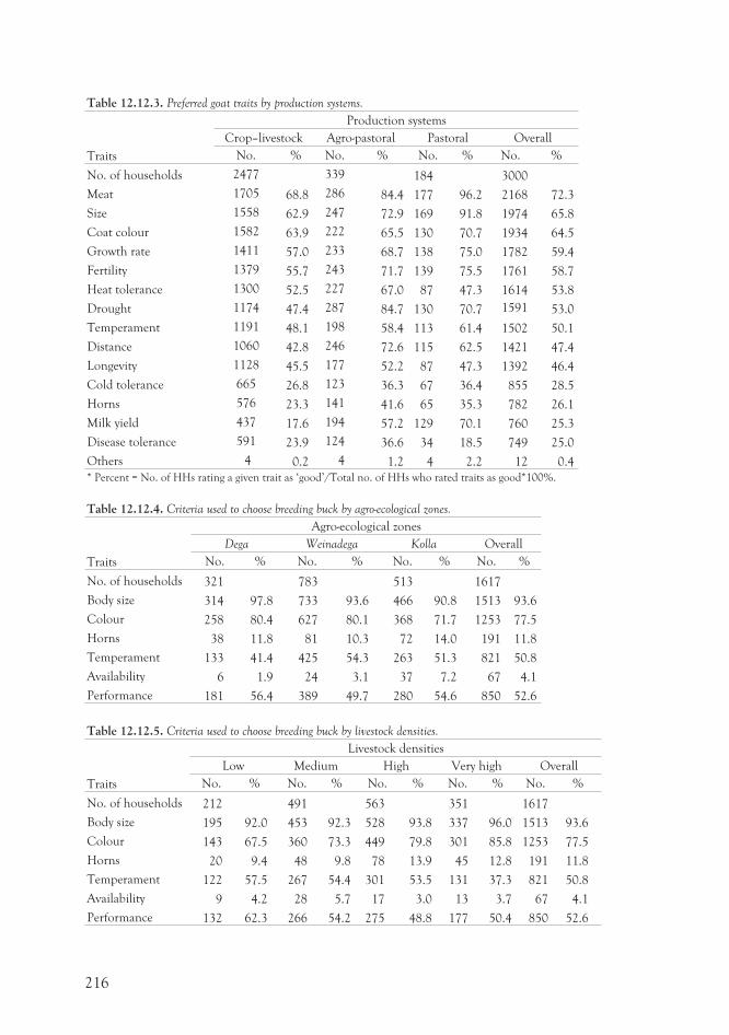
Table 12.12.3. Preferred goat traits by production systems.
Traits
Production systems
Crop–livestock Agro-pastoral Pastoral Overall
No. % No. % No. % No. %
No. of households 2477 339 184 3000
Meat 1705 68.8 286 84.4 177 96.2 2168 72.3
Size 1558 62.9 247 72.9 169 91.8 1974 65.8
Coat colour 1582 63.9 222 65.5 130 70.7 1934 64.5
Growth rate 1411 57.0 233 68.7 138 75.0 1782 59.4
Fertility 1379 55.7 243 71.7 139 75.5 1761 58.7
Heat tolerance 1300 52.5 227 67.0 87 47.3 1614 53.8
Drought 1174 47.4 287 84.7 130 70.7 1591 53.0
Temperament 1191 48.1 198 58.4 113 61.4 1502 50.1
Distance 1060 42.8 246 72.6 115 62.5 1421 47.4
Longevity 1128 45.5 177 52.2 87 47.3 1392 46.4
Cold tolerance 665 26.8 123 36.3 67 36.4 855 28.5
Horns 576 23.3 141 41.6 65 35.3 782 26.1
Milk yield 437 17.6 194 57.2 129 70.1 760 25.3
Disease tolerance 591 23.9 124 36.6 34 18.5 749 25.0
Others 4 0.2 4 1.2 4 2.2 12 0.4
* Percent = No. of HHs rating a given trait as ‘good’/Total no. of HHs who rated traits as good*100%.
Table 12.12.4. Criteria used to choose breeding buck by agro-ecological zones.
Traits
Agro-ecological zones
Dega Weinadega Kolla Overall
No. % No. % No. % No. %
No. of households 321 783 513 1617
Body size 314 97.8 733 93.6 466 90.8 1513 93.6
Colour 258 80.4 627 80.1 368 71.7 1253 77.5
Horns 38 11.8 81 10.3 72 14.0 191 11.8
Temperament 133 41.4 425 54.3 263 51.3 821 50.8
Availability 6 1.9 24 3.1 37 7.2 67 4.1
Performance 181 56.4 389 49.7 280 54.6 850 52.6
Table 12.12.5. Criteria used to choose breeding buck by livestock densities.
Traits
Livestock densities
Low Medium High Very high Overall
No. % No. % No. % No. % No. %
No. of households 212 491 563 351 1617
Body size 195 92.0 453 92.3 528 93.8 337 96.0 1513 93.6
Colour 143 67.5 360 73.3 449 79.8 301 85.8 1253 77.5
Horns 20 9.4 48 9.8 78 13.9 45 12.8 191 11.8
Temperament 122 57.5 267 54.4 301 53.5 131 37.3 821 50.8
Availability 9 4.2 28 5.7 17 3.0 13 3.7 67 4.1
Performance 132 62.3 266 54.2 275 48.8 177 50.4 850 52.6
216
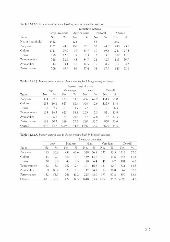
Table 12.12.6. Criteria used to choose breeding buck by production systems.
Traits
Production systems
Crop–livestock Agro-pastoral Pastoral Overall
No. % No. % No. % No. %
No. of households 1422 124 56 1602
Body size 1337 94.0 108 87.1 53 94.6 1498 93.5
Colour 1123 79.0 79 63.7 39 69.6 1241 77.5
Horns 178 12.5 9 7.3 2 3.6 189 11.8
Temperament 748 52.6 43 34.7 24 42.9 815 50.9
Availability 44 3.1 18 14.5 5 8.9 67 4.2
Performance 709 49.9 96 77.4 38 67.9 843 52.6
Table 12.12.7. Primary criteria used to choose breeding buck by agro-ecological zones.
Traits
Agro-ecological zones
Dega Weinadega Kolla Overall
No. % No. % No. % No. %
Body size 314 57.0 733 53.3 466 62.9 1513 57.0
Colour 258 10.1 627 12.4 368 10.6 1253 11.4
Horns 38 7.9 81 3.7 72 8.3 191 6.3
Temperament 133 14.3 425 18.8 263 5.3 821 13.8
Availability 6 66.7 24 29.2 37 37.8 67 37.3
Performance 181 50.3 389 57.3 280 50.7 850 53.6
Overall 930 34.6 2279 34.3 1486 34.2 4695 34.3
Table 12.12.8. Primary criteria used to choose breeding buck by livestock densities.
Traits
Livestock densities
Low Medium High Very high Overall
No. % No. % No. % No. % No. %
Body size 195 50.8 453 63.4 528 56.8 337 52.5 1513 57.0
Colour 143 9.1 360 9.4 449 13.6 301 11.6 1253 11.4
Horns 20 0.0 48 8.3 78 6.4 45 6.7 191 6.3
Temperament 122 13.1 267 12.4 301 16.6 131 10.7 821 13.8
Availability 9 88.9 28 7.1 17 64.7 13 30.8 67 37.3
Performance 132 55.3 266 49.2 275 48.0 177 67.8 850 53.6
Overall 621 33.7 1422 34.5 1648 33.9 1004 35.2 4695 34.3
217
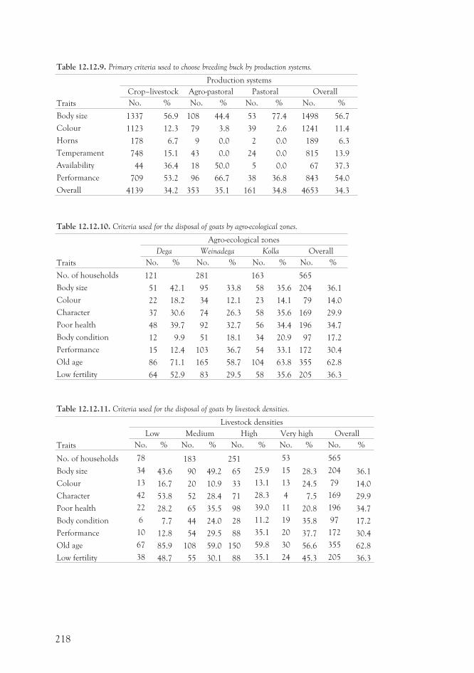
Table 12.12.9. Primary criteria used to choose breeding buck by production systems.
Traits
Production systems
Crop–livestock Agro-pastoral Pastoral Overall
No. % No. % No. % No. %
Body size 1337 56.9 108 44.4 53 77.4 1498 56.7
Colour 1123 12.3 79 3.8 39 2.6 1241 11.4
Horns 178 6.7 9 0.0 2 0.0 189 6.3
Temperament 748 15.1 43 0.0 24 0.0 815 13.9
Availability 44 36.4 18 50.0 5 0.0 67 37.3
Performance 709 53.2 96 66.7 38 36.8 843 54.0
Overall 4139 34.2 353 35.1 161 34.8 4653 34.3
Table 12.12.10. Criteria used for the disposal of goats by agro-ecological zones.
Traits
Agro-ecological zones
Dega Weinadega Kolla Overall
No. % No. % No. % No. %
No. of households 121 281 163 565
Body size 51 42.1 95 33.8 58 35.6 204 36.1
Colour 22 18.2 34 12.1 23 14.1 79 14.0
Character 37 30.6 74 26.3 58 35.6 169 29.9
Poor health 48 39.7 92 32.7 56 34.4 196 34.7
Body condition 12 9.9 51 18.1 34 20.9 97 17.2
Performance 15 12.4 103 36.7 54 33.1 172 30.4
Old age 86 71.1 165 58.7 104 63.8 355 62.8
Low fertility 64 52.9 83 29.5 58 35.6 205 36.3
Table 12.12.11. Criteria used for the disposal of goats by livestock densities.
Traits
Livestock densities
Low Medium High Very high Overall
No. % No. % No. % No. % No. %
No. of households 78 183 251 53 565
Body size 34 43.6 90 49.2 65 25.9 15 28.3 204 36.1
Colour 13 16.7 20 10.9 33 13.1 13 24.5 79 14.0
Character 42 53.8 52 28.4 71 28.3 4 7.5 169 29.9
Poor health 22 28.2 65 35.5 98 39.0 11 20.8 196 34.7
Body condition 6 7.7 44 24.0 28 11.2 19 35.8 97 17.2
Performance 10 12.8 54 29.5 88 35.1 20 37.7 172 30.4
Old age 67 85.9 108 59.0 150 59.8 30 56.6 355 62.8
Low fertility 38 48.7 55 30.1 88 35.1 24 45.3 205 36.3
218
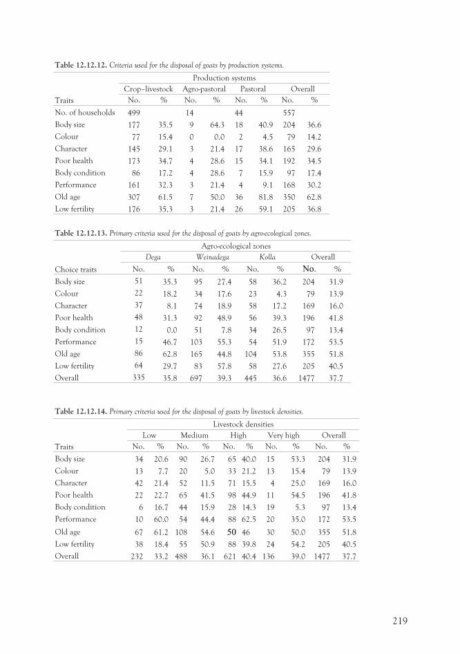
Table 12.12.12. Criteria used for the disposal of goats by production systems.
Traits
Production systems
Crop–livestock Agro-pastoral Pastoral Overall
No. % No. % No. % No. %
No. of households 499 14 44 557
Body size 177 35.5 9 64.3 18 40.9 204 36.6
Colour 77 15.4 0 0.0 2 4.5 79 14.2
Character 145 29.1 3 21.4 17 38.6 165 29.6
Poor health 173 34.7 4 28.6 15 34.1 192 34.5
Body condition 86 17.2 4 28.6 7 15.9 97 17.4
Performance 161 32.3 3 21.4 4 9.1 168 30.2
Old age 307 61.5 7 50.0 36 81.8 350 62.8
Low fertility 176 35.3 3 21.4 26 59.1 205 36.8
Table 12.12.13. Primary criteria used for the disposal of goats by agro-ecological zones.
Choice traits
Agro-ecological zones
Dega Weinadega Kolla Overall
No. % No. % No. % No. %
Body size 51 35.3 95 27.4 58 36.2 204 31.9
Colour 22 18.2 34 17.6 23 4.3 79 13.9
Character 37 8.1 74 18.9 58 17.2 169 16.0
Poor health 48 31.3 92 48.9 56 39.3 196 41.8
Body condition 12 0.0 51 7.8 34 26.5 97 13.4
Performance 15 46.7 103 55.3 54 51.9 172 53.5
Old age 86 62.8 165 44.8 104 53.8 355 51.8
Low fertility 64 29.7 83 57.8 58 27.6 205 40.5
Overall 335 35.8 697 39.3 445 36.6 1477 37.7
Table 12.12.14. Primary criteria used for the disposal of goats by livestock densities.
Traits
Livestock densities
Low Medium High Very high Overall
No. % No. % No. % No. % No. %
Body size 34 20.6 90 26.7 65 40.0 15 53.3 204 31.9
Colour 13 7.7 20 5.0 33 21.2 13 15.4 79 13.9
Character 42 21.4 52 11.5 71 15.5 4 25.0 169 16.0
Poor health 22 22.7 65 41.5 98 44.9 11 54.5 196 41.8
Body condition 6 16.7 44 15.9 28 14.3 19 5.3 97 13.4
Performance 10 60.0 54 44.4 88 62.5 20 35.0 172 53.5
Old age 67 61.2 108 54.6 50 46 30 50.0 355 51.8
Low fertility 38 18.4 55 50.9 88 39.8 24 54.2 205 40.5
Overall 232 33.2 488 36.1 621 40.4 136 39.0 1477 37.7
219
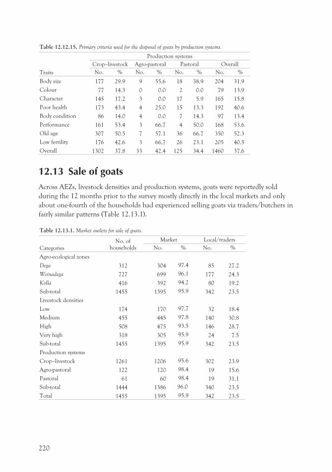
Table 12.12.15. Primary criteria used for the disposal of goats by production systems.
Traits
Production systems
Crop–livestock Agro-pastoral Pastoral Overall
No. % No. % No. % No. %
Body size 177 29.9 9 55.6 18 38.9 204 31.9
Colour 77 14.3 0 0.0 2 0.0 79 13.9
Character 145 17.2 3 0.0 17 5.9 165 15.8
Poor health 173 43.4 4 25.0 15 13.3 192 40.6
Body condition 86 14.0 4 0.0 7 14.3 97 13.4
Performance 161 53.4 3 66.7 4 50.0 168 53.6
Old age 307 50.5 7 57.1 36 66.7 350 52.3
Low fertility 176 42.6 3 66.7 26 23.1 205 40.5
Overall 1302 37.8 33 42.4 125 34.4 1460 37.6
12.13 Sale of goatsAcross AEZs, livestock densities and production systems, goats were reportedly sold
during the 12 months prior to the survey mostly directly in the local markets and only
about one-fourth of the households had experienced selling goats via traders/butchers in
fairly similar patterns (Table 12.13.1).
Table 12.13.1. Market outlets for sale of goats.
Categories
No. ofhouseholds
Market Local/traders
No. % No. %
Agro-ecological zones
Dega 312 304 97.4 85 27.2
Weinadega 727 699 96.1 177 24.3
Kolla 416 392 94.2 80 19.2
Sub-total 1455 1395 95.9 342 23.5
Livestock densities
Low 174 170 97.7 32 18.4
Medium 455 445 97.8 140 30.8
High 508 475 93.5 146 28.7
Very high 318 305 95.9 24 7.5
Sub-total 1455 1395 95.9 342 23.5
Production systems
Crop–livestock 1261 1206 95.6 302 23.9
Agro-pastoral 122 120 98.4 19 15.6
Pastoral 61 60 98.4 19 31.1
Sub-total 1444 1386 96.0 340 23.5
Total 1455 1395 95.9 342 23.5
220
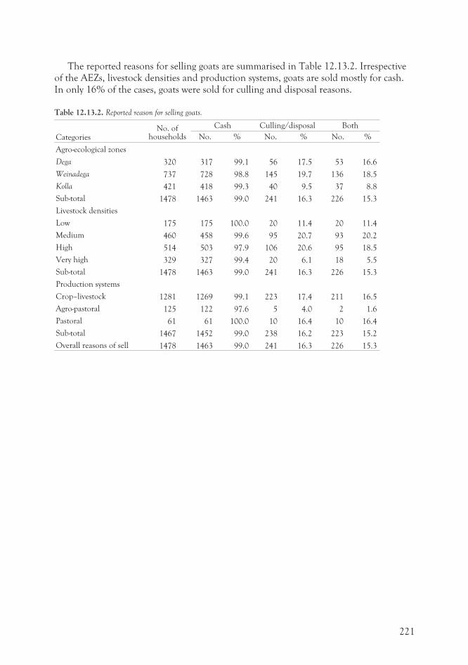
The reported reasons for selling goats are summarised in Table 12.13.2. Irrespectiveof the AEZs, livestock densities and production systems, goats are sold mostly for cash.In only 16% of the cases, goats were sold for culling and disposal reasons.
Table 12.13.2. Reported reason for selling goats.
CategoriesNo. of
households
Cash Culling/disposal Both
No. % No. % No. %
Agro-ecological zones
Dega 320 317 99.1 56 17.5 53 16.6
Weinadega 737 728 98.8 145 19.7 136 18.5
Kolla 421 418 99.3 40 9.5 37 8.8
Sub-total 1478 1463 99.0 241 16.3 226 15.3
Livestock densities
Low 175 175 100.0 20 11.4 20 11.4
Medium 460 458 99.6 95 20.7 93 20.2
High 514 503 97.9 106 20.6 95 18.5
Very high 329 327 99.4 20 6.1 18 5.5
Sub-total 1478 1463 99.0 241 16.3 226 15.3
Production systems
Crop–livestock 1281 1269 99.1 223 17.4 211 16.5
Agro-pastoral 125 122 97.6 5 4.0 2 1.6
Pastoral 61 61 100.0 10 16.4 10 16.4
Sub-total 1467 1452 99.0 238 16.2 223 15.2
Overall reasons of sell 1478 1463 99.0 241 16.3 226 15.3
221
13 Secondary species13.1 Chicken
A total of 3231 households, or about 59% of the total sample across Oromiya
Regional State, maintain chicken for various purposes. The number of chicken in
current holdings of these households was about 20 thousand birds, which gives an
average holding of 6.2 chickens per household. The ownership ratio across admin-
istrative zones varies from 32% in East Hararge to 81% in West Wellega (Table
9.1.1).
13.1.1 Purposes of keeping chickens
Chickens are mainly kept for egg (females), reproduction, meat, income and
savings. Egg production appears to be not a major reason for keeping male chick-
ens. Other purposes of keeping chickens include socio-cultural role (dowry,
ceremonies, wealth status), manure and feathers (Tables 13.1.1a, b and c). The
relative importance of each of the purposes is generally similar across AEZs,
livestock densities and production systems, except in the cases of income and meat
production. The role of chicken in income generation was more emphasised in
crop–livestock and agro-pastoral areas than in pastoral areas, and in medium to
high livestock density areas than in low livestock density areas, where instead meat
production was rated better. Similarly, pastoral areas have less frequent socio-
cultural reasons for keeping chickens, as these appear to be better served by other
livestock species.
222
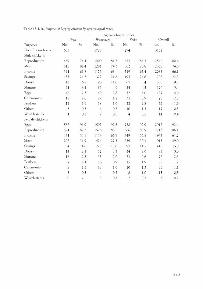
Table 13.1.1a. Purposes of keeping chickens by agro-ecological zones.
Purposes
Agro-ecological zones
Dega Weinadega Kolla Overall
No. % No. % No. % No. %
No. of households 633 1725 794 3152
Male chickens
Reproduction 469 74.1 1400 81.2 671 84.5 2540 80.6
Meat 515 81.4 1281 74.3 562 70.8 2358 74.8
Income 391 61.8 1173 68 519 65.4 2083 66.1
Savings 135 21.3 372 21.6 195 24.6 702 22.3
Dowry 43 6.8 190 11.0 67 8.4 300 9.5
Manure 51 8.1 85 4.9 34 4.3 170 5.4
Eggs 46 7.3 49 2.8 32 4.0 127 4.0
Ceremonies 18 2.8 29 1.7 31 3.9 78 2.5
Feathers 12 1.9 18 1.0 22 2.8 52 1.6
Others 3 0.5 4 0.2 10 1.3 17 0.5
Wealth status 1 0.2 9 0.5 4 0.5 14 0.4
Female chickens
Eggs 582 91.9 1592 92.3 738 92.9 2912 92.4
Reproduction 521 82.3 1526 88.5 666 83.9 2713 86.1
Income 341 53.9 1154 66.9 449 56.5 1944 61.7
Meat 202 31.9 474 27.5 239 30.1 915 29.0
Savings 94 14.8 225 13.0 91 11.5 410 13.0
Dowry 14 2.2 57 3.3 24 3.0 95 3.0
Manure 16 2.5 35 2.0 21 2.6 72 2.3
Feathers 7 1.1 16 0.9 15 1.9 38 1.2
Ceremonies 8 1.3 18 1.0 10 1.3 36 1.1
Others 3 0.5 4 0.2 8 1.0 15 0.5
Wealth status 0 – 3 0.2 2 0.3 5 0.2
223
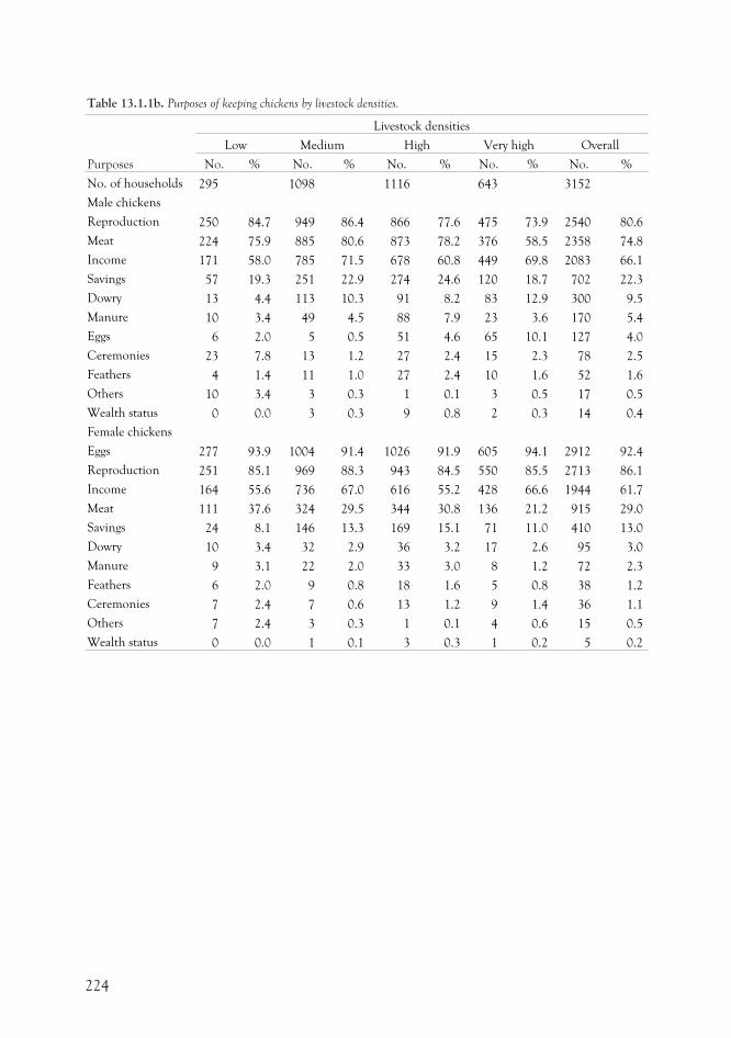
Table 13.1.1b. Purposes of keeping chickens by livestock densities.
Purposes
Livestock densities
Low Medium High Very high Overall
No. % No. % No. % No. % No. %
No. of households 295 1098 1116 643 3152
Male chickens
Reproduction 250 84.7 949 86.4 866 77.6 475 73.9 2540 80.6
Meat 224 75.9 885 80.6 873 78.2 376 58.5 2358 74.8
Income 171 58.0 785 71.5 678 60.8 449 69.8 2083 66.1
Savings 57 19.3 251 22.9 274 24.6 120 18.7 702 22.3
Dowry 13 4.4 113 10.3 91 8.2 83 12.9 300 9.5
Manure 10 3.4 49 4.5 88 7.9 23 3.6 170 5.4
Eggs 6 2.0 5 0.5 51 4.6 65 10.1 127 4.0
Ceremonies 23 7.8 13 1.2 27 2.4 15 2.3 78 2.5
Feathers 4 1.4 11 1.0 27 2.4 10 1.6 52 1.6
Others 10 3.4 3 0.3 1 0.1 3 0.5 17 0.5
Wealth status 0 0.0 3 0.3 9 0.8 2 0.3 14 0.4
Female chickens
Eggs 277 93.9 1004 91.4 1026 91.9 605 94.1 2912 92.4
Reproduction 251 85.1 969 88.3 943 84.5 550 85.5 2713 86.1
Income 164 55.6 736 67.0 616 55.2 428 66.6 1944 61.7
Meat 111 37.6 324 29.5 344 30.8 136 21.2 915 29.0
Savings 24 8.1 146 13.3 169 15.1 71 11.0 410 13.0
Dowry 10 3.4 32 2.9 36 3.2 17 2.6 95 3.0
Manure 9 3.1 22 2.0 33 3.0 8 1.2 72 2.3
Feathers 6 2.0 9 0.8 18 1.6 5 0.8 38 1.2
Ceremonies 7 2.4 7 0.6 13 1.2 9 1.4 36 1.1
Others 7 2.4 3 0.3 1 0.1 4 0.6 15 0.5
Wealth status 0 0.0 1 0.1 3 0.3 1 0.2 5 0.2
224
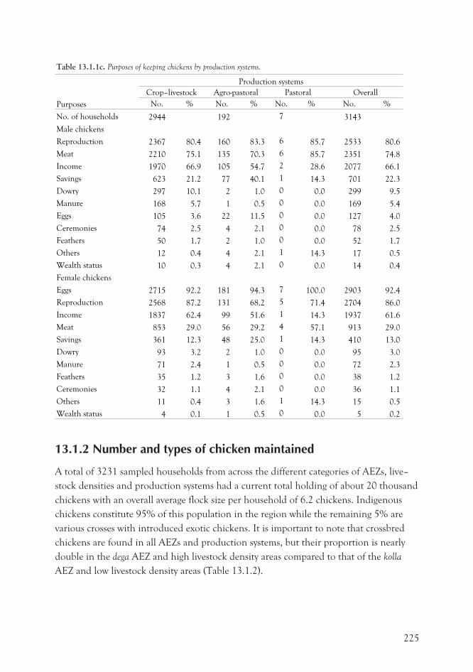
Table 13.1.1c. Purposes of keeping chickens by production systems.
Purposes
Production systems
Crop–livestock Agro-pastoral Pastoral Overall
No. % No. % No. % No. %
No. of households 2944 192 7 3143
Male chickens
Reproduction 2367 80.4 160 83.3 6 85.7 2533 80.6
Meat 2210 75.1 135 70.3 6 85.7 2351 74.8
Income 1970 66.9 105 54.7 2 28.6 2077 66.1
Savings 623 21.2 77 40.1 1 14.3 701 22.3
Dowry 297 10.1 2 1.0 0 0.0 299 9.5
Manure 168 5.7 1 0.5 0 0.0 169 5.4
Eggs 105 3.6 22 11.5 0 0.0 127 4.0
Ceremonies 74 2.5 4 2.1 0 0.0 78 2.5
Feathers 50 1.7 2 1.0 0 0.0 52 1.7
Others 12 0.4 4 2.1 1 14.3 17 0.5
Wealth status 10 0.3 4 2.1 0 0.0 14 0.4
Female chickens
Eggs 2715 92.2 181 94.3 7 100.0 2903 92.4
Reproduction 2568 87.2 131 68.2 5 71.4 2704 86.0
Income 1837 62.4 99 51.6 1 14.3 1937 61.6
Meat 853 29.0 56 29.2 4 57.1 913 29.0
Savings 361 12.3 48 25.0 1 14.3 410 13.0
Dowry 93 3.2 2 1.0 0 0.0 95 3.0
Manure 71 2.4 1 0.5 0 0.0 72 2.3
Feathers 35 1.2 3 1.6 0 0.0 38 1.2
Ceremonies 32 1.1 4 2.1 0 0.0 36 1.1
Others 11 0.4 3 1.6 1 14.3 15 0.5
Wealth status 4 0.1 1 0.5 0 0.0 5 0.2
13.1.2 Number and types of chicken maintained
A total of 3231 sampled households from across the different categories of AEZs, live–
stock densities and production systems had a current total holding of about 20 thousand
chickens with an overall average flock size per household of 6.2 chickens. Indigenous
chickens constitute 95% of this population in the region while the remaining 5% are
various crosses with introduced exotic chickens. It is important to note that crossbred
chickens are found in all AEZs and production systems, but their proportion is nearly
double in the dega AEZ and high livestock density areas compared to that of the kolla
AEZ and low livestock density areas (Table 13.1.2).
225
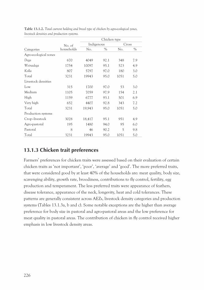
Table 13.1.2. Total current holding and breed type of chicken by agro-ecological zones,
livestock densities and production systems.
CategoriesNo. of
households
Chicken type
Indigenous Cross
No. % No. %
Agro-ecological zones
Dega 670 4049 92.1 348 7.9
Weinadega 1754 10097 95.1 523 4.9
Kolla 807 5797 97.0 180 3.0
Total 3231 19943 95.0 1051 5.0
Livestock densities
Low 315 1700 97.0 53 3.0
Medium 1105 7059 97.9 154 2.1
High 1159 6777 93.1 501 6.9
Very high 652 4407 92.8 343 7.2
Total 3231 19,943 95.0 1051 5.0
Production systems
Crop–livestock 3028 18,417 95.1 951 4.9
Agro-pastoral 195 1480 94.0 95 6.0
Pastoral 8 46 90.2 5 9.8
Total 3231 19943 95.0 1051 5.0
13.1.3 Chicken trait preferences
Farmers’ preferences for chicken traits were assessed based on their evaluation of certain
chicken traits as ‘not important’, ‘poor’, ‘average’ and ‘good’. The more preferred traits,
that were considered good by at least 40% of the households are: meat quality, body size,
scavenging ability, growth rate, broodiness, contributions to fly control, fertility, egg
production and temperament. The less preferred traits were appearance of feathers,
disease tolerance, appearance of the neck, longevity, heat and cold tolerances. These
patterns are generally consistent across AEZs, livestock density categories and production
systems (Tables 13.1.3a, b and c). Some notable exceptions are the higher than average
preference for body size in pastoral and agro-pastoral areas and the low preference for
meat quality in pastoral areas. The contribution of chicken in fly control received higher
emphasis in low livestock density areas.
226
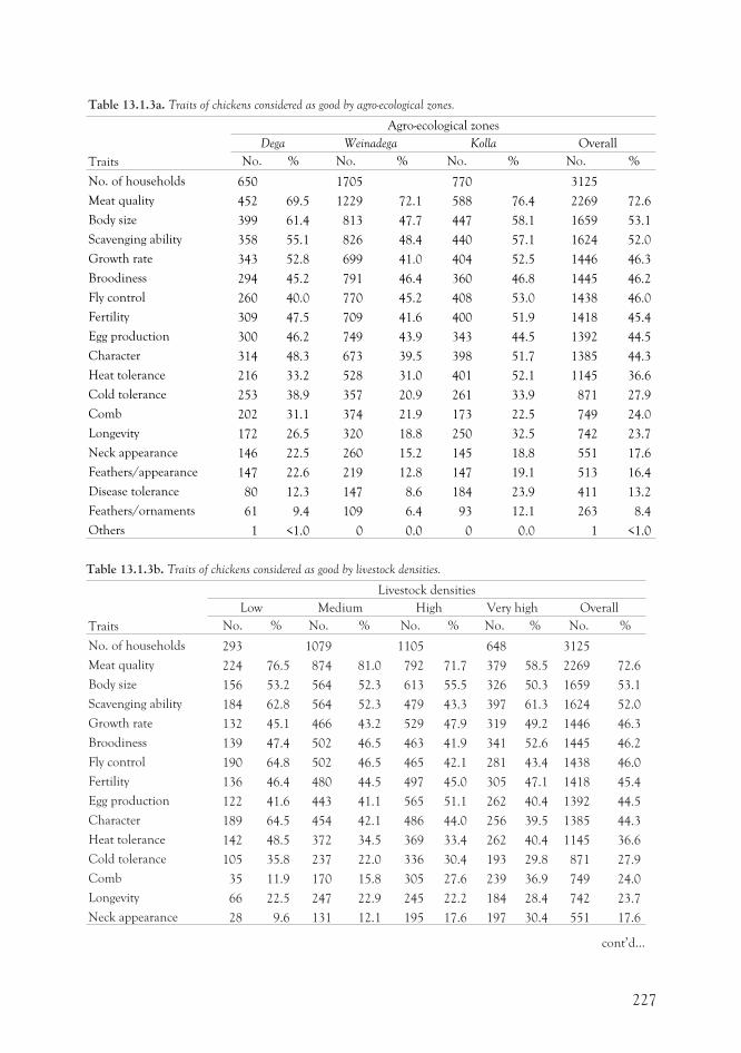
Table 13.1.3a. Traits of chickens considered as good by agro-ecological zones.
Traits
Agro-ecological zones
Dega Weinadega Kolla Overall
No. % No. % No. % No. %
No. of households 650 1705 770 3125
Meat quality 452 69.5 1229 72.1 588 76.4 2269 72.6
Body size 399 61.4 813 47.7 447 58.1 1659 53.1
Scavenging ability 358 55.1 826 48.4 440 57.1 1624 52.0
Growth rate 343 52.8 699 41.0 404 52.5 1446 46.3
Broodiness 294 45.2 791 46.4 360 46.8 1445 46.2
Fly control 260 40.0 770 45.2 408 53.0 1438 46.0
Fertility 309 47.5 709 41.6 400 51.9 1418 45.4
Egg production 300 46.2 749 43.9 343 44.5 1392 44.5
Character 314 48.3 673 39.5 398 51.7 1385 44.3
Heat tolerance 216 33.2 528 31.0 401 52.1 1145 36.6
Cold tolerance 253 38.9 357 20.9 261 33.9 871 27.9
Comb 202 31.1 374 21.9 173 22.5 749 24.0
Longevity 172 26.5 320 18.8 250 32.5 742 23.7
Neck appearance 146 22.5 260 15.2 145 18.8 551 17.6
Feathers/appearance 147 22.6 219 12.8 147 19.1 513 16.4
Disease tolerance 80 12.3 147 8.6 184 23.9 411 13.2
Feathers/ornaments 61 9.4 109 6.4 93 12.1 263 8.4
Others 1 <1.0 0 0.0 0 0.0 1 <1.0
Table 13.1.3b. Traits of chickens considered as good by livestock densities.
Traits
Livestock densities
Low Medium High Very high Overall
No. % No. % No. % No. % No. %
No. of households 293 1079 1105 648 3125
Meat quality 224 76.5 874 81.0 792 71.7 379 58.5 2269 72.6
Body size 156 53.2 564 52.3 613 55.5 326 50.3 1659 53.1
Scavenging ability 184 62.8 564 52.3 479 43.3 397 61.3 1624 52.0
Growth rate 132 45.1 466 43.2 529 47.9 319 49.2 1446 46.3
Broodiness 139 47.4 502 46.5 463 41.9 341 52.6 1445 46.2
Fly control 190 64.8 502 46.5 465 42.1 281 43.4 1438 46.0
Fertility 136 46.4 480 44.5 497 45.0 305 47.1 1418 45.4
Egg production 122 41.6 443 41.1 565 51.1 262 40.4 1392 44.5
Character 189 64.5 454 42.1 486 44.0 256 39.5 1385 44.3
Heat tolerance 142 48.5 372 34.5 369 33.4 262 40.4 1145 36.6
Cold tolerance 105 35.8 237 22.0 336 30.4 193 29.8 871 27.9
Comb 35 11.9 170 15.8 305 27.6 239 36.9 749 24.0
Longevity 66 22.5 247 22.9 245 22.2 184 28.4 742 23.7
Neck appearance 28 9.6 131 12.1 195 17.6 197 30.4 551 17.6
227
cont’d...
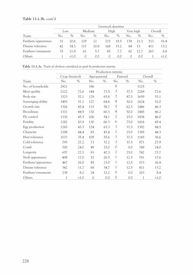
Traits
Livestock densities
Low Medium High Very high Overall
No. % No. % No. % No. % No. %
Feathers/appearance 31 10.6 129 12 215 19.5 138 21.3 513 16.4
Disease tolerance 42 14.3 117 10.8 168 15.2 84 13 411 13.2
Feathers/ornaments 35 11.9 61 5.7 85 7.7 82 12.7 263 8.4
Others 1 <1.0 0 0.0 0 0.0 0 0.0 1 <1.0
Table 13.1.3c. Traits of chickens considered as good by production systems.
Traits
Production systems
Crop–livestock Agro-pastoral Pastoral Overall
No. % No. % No. % No. %
No. of households 2921 196 8 3125
Meat quality 2122 72.6 144 73.5 3 37.5 2269 72.6
Body size 1523 52.1 129 65.8 7 87.5 1659 53.1
Scavenging ability 1493 51.1 127 64.8 4 50.0 1624 52.0
Growth rate 1326 45.4 115 58.7 5 62.5 1446 46.3
Broodiness 1311 44.9 130 66.3 4 50.0 1445 46.2
Fly control 1330 45.5 106 54.1 2 25.0 1438 46.0
Fertility 1282 43.9 130 66.3 6 75.0 1418 45.4
Egg production 1265 43.3 124 63.3 3 37.5 1392 44.5
Character 1298 44.4 85 43.4 2 25.0 1385 44.3
Heat tolerance 1033 35.4 109 55.6 3 37.5 1145 36.6
Cold tolerance 795 27.2 73 37.2 3 37.5 871 27.9
Comb 700 24.0 49 25.0 0 0.0 749 24.0
Longevity 657 22.5 83 42.3 2 25.0 742 23.7
Neck appearance 498 17.0 52 26.5 1 12.5 551 17.6
Feathers/appearance 467 16.0 45 23.0 1 12.5 513 16.4
Disease tolerance 342 11.7 68 34.7 1 12.5 411 13.2
Feathers/ornaments 239 8.2 24 12.2 0 0.0 263 8.4
Others 1 <1.0 0 0.0 0 0.0 1 <1.0
228
Table 13.1.3b. cont’d
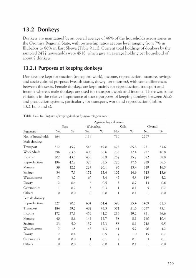
13.2 DonkeysDonkeys are maintained by an overall average of 46% of the households across zones in
the Oromiya Regional State, with ownership ratios at zone level ranging from 7% in
Illubabor to 86% in East Shewa (Table 9.1.1). Current total holdings of donkeys by the
sampled 2477 households were 4918, which give an average holding per household of
about 2 donkeys.
13.2.1 Purposes of keeping donkeys
Donkeys are kept for traction (transport, work), income, reproduction, manure, savings
and socio-cultural purposes (wealth status, dowry, ceremonies), with some differences
between the sexes. Female donkeys are kept mainly for reproduction, transport and
income whereas male donkeys are used for transport, work and income. There was some
variation in the relative importance of those purposes of keeping donkeys between AEZs
and production systems, particularly for transport, work and reproduction (Tables
13.2.1a, b and c).
Table 13.2.1a. Purposes of keeping donkeys by agro-ecological zones.
Purposes
Agro-ecological zones
Dega Weinadega Kolla Overall
No. % No. % No. % No. %
No. of households 464 1114 719 2297
Male donkeys
Transport 212 45.7 546 49.0 473 65.8 1231 53.6
Work/draft 296 63.8 408 36.6 233 32.4 937 40.8
Income 202 43.5 433 38.9 257 35.7 892 38.8
Reproduction 196 42.2 373 33.5 270 37.6 839 36.5
Manure 59 12.7 224 20.1 96 13.4 379 16.5
Savings 34 7.3 172 15.4 107 14.9 313 13.6
Wealth status 17 3.7 60 5.4 42 5.8 119 5.2
Dowry 2 0.4 6 0.5 5 0.7 13 0.6
Ceremonies 1 0.2 3 0.3 1 0.1 5 0.2
Others 0 0.0 0 0.0 1 0.1 1 0.0
Female donkeys
Reproduction 327 70.5 684 61.4 398 55.4 1409 61.3
Transport 184 39.7 482 43.3 371 51.6 1037 45.1
Income 172 37.1 459 41.2 210 29.2 841 36.6
Manure 40 8.6 142 12.7 58 8.1 240 10.4
Savings 23 5.0 137 12.3 58 8.1 218 9.5
Wealth status 7 1.5 48 4.3 41 5.7 96 4.2
Dowry 2 0.4 6 0.5 7 1.0 15 0.7
Ceremonies 0 0.0 1 0.1 2 0.3 3 0.1
Others 0 0.0 0 0.0 1 0.1 1 0.0
229
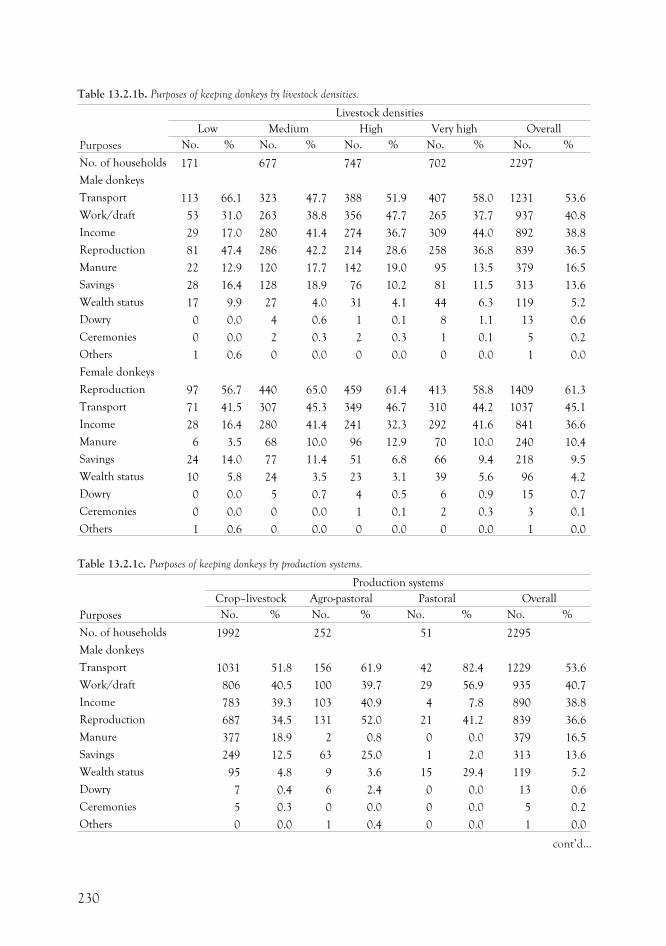
Table 13.2.1b. Purposes of keeping donkeys by livestock densities.
Purposes
Livestock densities
Low Medium High Very high Overall
No. % No. % No. % No. % No. %
No. of households 171 677 747 702 2297
Male donkeys
Transport 113 66.1 323 47.7 388 51.9 407 58.0 1231 53.6
Work/draft 53 31.0 263 38.8 356 47.7 265 37.7 937 40.8
Income 29 17.0 280 41.4 274 36.7 309 44.0 892 38.8
Reproduction 81 47.4 286 42.2 214 28.6 258 36.8 839 36.5
Manure 22 12.9 120 17.7 142 19.0 95 13.5 379 16.5
Savings 28 16.4 128 18.9 76 10.2 81 11.5 313 13.6
Wealth status 17 9.9 27 4.0 31 4.1 44 6.3 119 5.2
Dowry 0 0.0 4 0.6 1 0.1 8 1.1 13 0.6
Ceremonies 0 0.0 2 0.3 2 0.3 1 0.1 5 0.2
Others 1 0.6 0 0.0 0 0.0 0 0.0 1 0.0
Female donkeys
Reproduction 97 56.7 440 65.0 459 61.4 413 58.8 1409 61.3
Transport 71 41.5 307 45.3 349 46.7 310 44.2 1037 45.1
Income 28 16.4 280 41.4 241 32.3 292 41.6 841 36.6
Manure 6 3.5 68 10.0 96 12.9 70 10.0 240 10.4
Savings 24 14.0 77 11.4 51 6.8 66 9.4 218 9.5
Wealth status 10 5.8 24 3.5 23 3.1 39 5.6 96 4.2
Dowry 0 0.0 5 0.7 4 0.5 6 0.9 15 0.7
Ceremonies 0 0.0 0 0.0 1 0.1 2 0.3 3 0.1
Others 1 0.6 0 0.0 0 0.0 0 0.0 1 0.0
Table 13.2.1c. Purposes of keeping donkeys by production systems.
Purposes
Production systems
Crop–livestock Agro-pastoral Pastoral Overall
No. % No. % No. % No. %
No. of households 1992 252 51 2295
Male donkeys
Transport 1031 51.8 156 61.9 42 82.4 1229 53.6
Work/draft 806 40.5 100 39.7 29 56.9 935 40.7
Income 783 39.3 103 40.9 4 7.8 890 38.8
Reproduction 687 34.5 131 52.0 21 41.2 839 36.6
Manure 377 18.9 2 0.8 0 0.0 379 16.5
Savings 249 12.5 63 25.0 1 2.0 313 13.6
Wealth status 95 4.8 9 3.6 15 29.4 119 5.2
Dowry 7 0.4 6 2.4 0 0.0 13 0.6
Ceremonies 5 0.3 0 0.0 0 0.0 5 0.2
Others 0 0.0 1 0.4 0 0.0 1 0.0
230
cont’d...
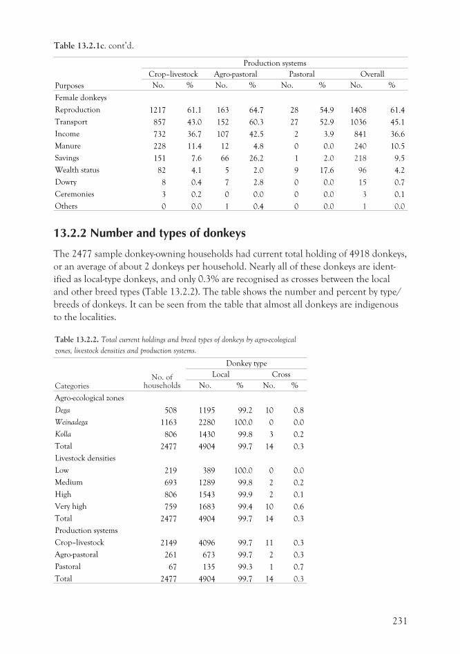
Purposes
Production systems
Crop–livestock Agro-pastoral Pastoral Overall
No. % No. % No. % No. %
Female donkeys
Reproduction 1217 61.1 163 64.7 28 54.9 1408 61.4
Transport 857 43.0 152 60.3 27 52.9 1036 45.1
Income 732 36.7 107 42.5 2 3.9 841 36.6
Manure 228 11.4 12 4.8 0 0.0 240 10.5
Savings 151 7.6 66 26.2 1 2.0 218 9.5
Wealth status 82 4.1 5 2.0 9 17.6 96 4.2
Dowry 8 0.4 7 2.8 0 0.0 15 0.7
Ceremonies 3 0.2 0 0.0 0 0.0 3 0.1
Others 0 0.0 1 0.4 0 0.0 1 0.0
13.2.2 Number and types of donkeys
The 2477 sample donkey-owning households had current total holding of 4918 donkeys,
or an average of about 2 donkeys per household. Nearly all of these donkeys are ident-
ified as local-type donkeys, and only 0.3% are recognised as crosses between the local
and other breed types (Table 13.2.2). The table shows the number and percent by type/
breeds of donkeys. It can be seen from the table that almost all donkeys are indigenous
to the localities.
Table 13.2.2. Total current holdings and breed types of donkeys by agro-ecological
zones, livestock densities and production systems.
CategoriesNo. of
households
Donkey type
Local Cross
No. % No. %
Agro-ecological zones
Dega 508 1195 99.2 10 0.8
Weinadega 1163 2280 100.0 0 0.0
Kolla 806 1430 99.8 3 0.2
Total 2477 4904 99.7 14 0.3
Livestock densities
Low 219 389 100.0 0 0.0
Medium 693 1289 99.8 2 0.2
High 806 1543 99.9 2 0.1
Very high 759 1683 99.4 10 0.6
Total 2477 4904 99.7 14 0.3
Production systems
Crop–livestock 2149 4096 99.7 11 0.3
Agro-pastoral 261 673 99.7 2 0.3
Pastoral 67 135 99.3 1 0.7
Total 2477 4904 99.7 14 0.3
231
Table 13.2.1c. cont’d.
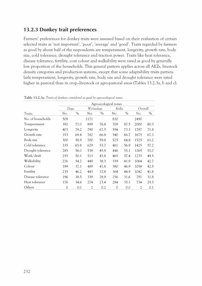
13.2.3 Donkey trait preferences
Farmers’ preferences for donkey traits were assessed based on their evaluation of certain
selected traits as ‘not important’, ‘poor’, ‘average’ and ‘good’. Traits regarded by farmers
as good by about half of the respondents are temperament, longevity, growth rate, body
size, cold tolerance, drought tolerance and traction power. Traits like heat tolerance,
disease tolerance, fertility, coat colour and walkability were rated as good by generally
low proportion of the households. This general pattern applies across all AEZs, livestock
density categories and production systems, except that some adaptability traits particu-
larly temperament, longevity, growth rate, body size and drought tolerance were rated
higher in pastoral than in crop–livestock or agro-pastoral areas (Tables 13.2.3a, b and c).
Table 13.2.3a. Traits of donkeys considered as good by agro-ecological zones.
Traits
Agro-ecological zones
Dega Weinadega Kolla Overall
No. % No. % No. % No. %
No. of households 509 1171 810 2490
Temperament 392 77.0 899 76.8 709 87.5 2000 80.3
Longevity 403 79.2 790 67.5 594 73.3 1787 71.8
Growth rate 353 69.4 782 66.8 540 66.7 1675 67.3
Body size 300 58.9 700 59.8 525 64.8 1525 61.2
Cold tolerance 335 65.8 629 53.7 461 56.9 1425 57.2
Drought tolerance 285 56.0 538 45.9 446 55.1 1269 51.0
Work/draft 255 50.1 513 43.8 465 57.4 1233 49.5
Walkability 276 54.2 449 38.3 339 41.9 1064 42.7
Colour 189 37.1 489 41.8 380 46.9 1058 42.5
Fertility 235 46.2 443 37.8 364 44.9 1042 41.8
Disease tolerance 196 38.5 339 28.9 256 31.6 791 31.8
Heat tolerance 176 34.6 274 23.4 284 35.1 734 29.5
Others 0 0.0 2 0.2 0 0.0 2 0.1
232
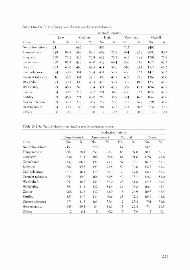
Table 13.2.3b. Traits of donkeys considered as good by livestock densities.
Traits
Livestock densities
Low Medium High Very high Overall
No. % No. % No. % No. % No. %
No. of households 211 693 803 783 2490
Temperament 179 84.8 569 82.1 608 75.7 644 82.2 2000 80.3
Longevity 150 71.1 525 75.8 627 78.1 485 61.9 1787 71.8
Growth rate 180 85.3 478 69.0 517 64.4 500 63.9 1675 67.3
Body size 133 63.0 468 67.5 414 51.6 510 65.1 1525 61.2
Cold tolerance 124 58.8 384 55.4 431 53.7 486 62.1 1425 57.2
Drought tolerance 116 55.0 361 52.1 383 47.7 409 52.2 1269 51.0
Work/draft 123 58.3 300 43.3 425 52.9 385 49.2 1233 49.5
Walkability 99 46.9 245 35.4 351 43.7 369 47.1 1064 42.7
Colour 84 39.8 272 39.2 294 36.6 408 52.1 1058 42.5
Fertility 99 46.9 291 42.0 288 35.9 364 46.5 1042 41.8
Disease tolerance 69 32.7 218 31.5 217 27.0 287 36.7 791 31.8
Heat tolerance 64 30.3 186 26.8 261 32.5 223 28.5 734 29.5
Others 0 0.0 0 0.0 2 0.2 0 0.0 2 0.1
Table 13.2.3c. Traits of donkeys considered as good by production systems.
Traits
Production systems
Crop–livestock Agro-pastoral Pastoral Overall
No. % No. % No. % No. %
No. of households 2153 270 67 2490
Temperament 1682 78.1 253 93.7 65 97.0 2000 80.3
Longevity 1538 71.4 188 69.6 61 91.0 1787 71.8
Growth rate 1432 66.5 192 71.1 51 76.1 1675 67.3
Body size 1282 59.5 193 71.5 50 74.6 1525 61.2
Cold tolerance 1214 56.4 179 66.3 32 47.8 1425 57.2
Drought tolerance 1054 49.0 166 61.5 49 73.1 1269 51.0
Work/draft 1051 48.8 154 57.0 28 41.8 1233 49.5
Walkability 891 41.4 147 54.4 26 38.8 1064 42.7
Colour 908 42.2 132 48.9 18 26.9 1058 42.5
Fertility 883 41.0 134 49.6 25 37.3 1042 41.8
Disease tolerance 673 31.3 101 37.4 17 25.4 791 31.8
Heat tolerance 635 29.5 84 31.1 15 22.4 734 29.5
Others 2 0.1 0 0.0 0 0.0 2 0.1
233
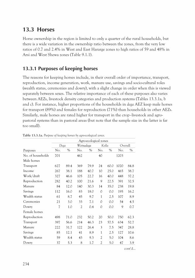
13.3 HorsesHorse ownership in the region is limited to only a quarter of the rural households, but
there is a wide variation in the ownership ratio between the zones, from the very low
ratios of 0.7 and 2.4% in West and East Hararge zones to high ratios of 59 and 48% in
Arsi and West Shewa zones (Table 9.1.1).
13.3.1 Purposes of keeping horses
The reasons for keeping horses include, in their overall order of importance, transport,
reproduction, income generation, work, manure use, savings and socio-cultural roles
(wealth status, ceremonies and dowry), with a slight change in order when this is viewed
separately between sexes. The relative importance of each of these purposes also varies
between AEZs, livestock density categories and production systems (Tables 13.3.1a, b
and c). For instance, higher proportions of the households in dega AEZ keep male horses
for transport (89%) and females for reproduction (71%) than households in other AEZs.
Similarly, male horses are rated higher for transport in the crop–livestock and agro-
pastoral systems than in pastoral areas (but note that the sample size in the latter is far
too small).
Table 13.3.1a. Purpose of keeping horses by agro-ecological zones.
Purposes
Agro-ecological zones
Dega Weinadega Kolla Overall
No. % No. % No. % No. %
No. of households 701 462 40 1203
Male horses
Transport 627 89.4 369 79.9 24 60.0 1020 84.8
Income 267 38.1 188 40.7 10 25.0 465 38.7
Work/draft 327 46.6 105 22.7 16 40.0 448 37.2
Reproduction 282 40.2 100 21.6 9 22.5 391 32.5
Manure 84 12.0 140 30.3 14 35.0 238 19.8
Savings 112 16.0 83 18.0 0 0.0 195 16.2
Wealth status 61 8.7 45 9.7 1 2.5 107 8.9
Ceremonies 21 3.0 33 7.1 0 0.0 54 4.5
Dowry 7 1.0 2 0.4 0 0.0 9 0.7
Female horses
Reproduction 498 71.0 232 50.2 20 50.0 750 62.3
Transport 397 56.6 214 46.3 23 57.5 634 52.7
Manure 222 31.7 122 26.4 3 7.5 347 28.8
Savings 85 12.1 41 8.9 1 2.5 127 10.6
Wealth status 59 8.4 43 9.3 2 5.0 104 8.6
Dowry 37 5.3 8 1.7 2 5.0 47 3.9
234
cont’d...
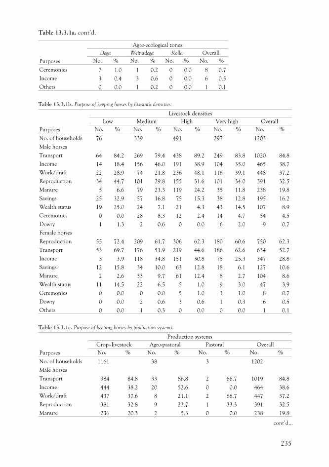
Purposes
Agro-ecological zones
Dega Weinadega Kolla Overall
No. % No. % No. % No. %
Ceremonies 7 1.0 1 0.2 0 0.0 8 0.7
Income 3 0.4 3 0.6 0 0.0 6 0.5
Others 0 0.0 1 0.2 0 0.0 1 0.1
Table 13.3.1b. Purpose of keeping horses by livestock densities.
Purposes
Livestock densities
Low Medium High Very high Overall
No. % No. % No. % No. % No. %
No. of households 76 339 491 297 1203
Male horses
Transport 64 84.2 269 79.4 438 89.2 249 83.8 1020 84.8
Income 14 18.4 156 46.0 191 38.9 104 35.0 465 38.7
Work/draft 22 28.9 74 21.8 236 48.1 116 39.1 448 37.2
Reproduction 34 44.7 101 29.8 155 31.6 101 34.0 391 32.5
Manure 5 6.6 79 23.3 119 24.2 35 11.8 238 19.8
Savings 25 32.9 57 16.8 75 15.3 38 12.8 195 16.2
Wealth status 19 25.0 24 7.1 21 4.3 43 14.5 107 8.9
Ceremonies 0 0.0 28 8.3 12 2.4 14 4.7 54 4.5
Dowry 1 1.3 2 0.6 0 0.0 6 2.0 9 0.7
Female horses
Reproduction 55 72.4 209 61.7 306 62.3 180 60.6 750 62.3
Transport 53 69.7 176 51.9 219 44.6 186 62.6 634 52.7
Income 3 3.9 118 34.8 151 30.8 75 25.3 347 28.8
Savings 12 15.8 34 10.0 63 12.8 18 6.1 127 10.6
Manure 2 2.6 33 9.7 61 12.4 8 2.7 104 8.6
Wealth status 11 14.5 22 6.5 5 1.0 9 3.0 47 3.9
Ceremonies 0 0.0 0 0.0 5 1.0 3 1.0 8 0.7
Dowry 0 0.0 2 0.6 3 0.6 1 0.3 6 0.5
Others 0 0.0 1 0.3 0 0.0 0 0.0 1 0.1
Table 13.3.1c. Purpose of keeping horses by production systems.
Purposes
Production systems
Crop–livestock Agro-pastoral Pastoral Overall
No. % No. % No. % No. %
No. of households 1161 38 3 1202
Male horses
Transport 984 84.8 33 86.8 2 66.7 1019 84.8
Income 444 38.2 20 52.6 0 0.0 464 38.6
Work/draft 437 37.6 8 21.1 2 66.7 447 37.2
Reproduction 381 32.8 9 23.7 1 33.3 391 32.5
Manure 236 20.3 2 5.3 0 0.0 238 19.8
235
Table 13.3.1a. cont’d.
cont’d...
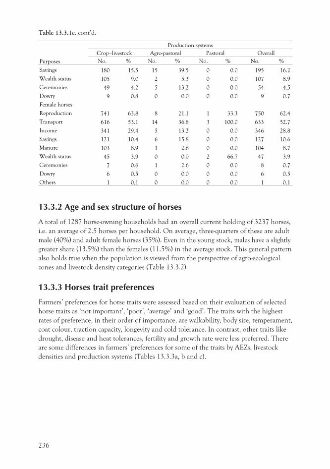
Purposes
Production systems
Crop–livestock Agro-pastoral Pastoral Overall
No. % No. % No. % No. %
Savings 180 15.5 15 39.5 0 0.0 195 16.2
Wealth status 105 9.0 2 5.3 0 0.0 107 8.9
Ceremonies 49 4.2 5 13.2 0 0.0 54 4.5
Dowry 9 0.8 0 0.0 0 0.0 9 0.7
Female horses
Reproduction 741 63.8 8 21.1 1 33.3 750 62.4
Transport 616 53.1 14 36.8 3 100.0 633 52.7
Income 341 29.4 5 13.2 0 0.0 346 28.8
Savings 121 10.4 6 15.8 0 0.0 127 10.6
Manure 103 8.9 1 2.6 0 0.0 104 8.7
Wealth status 45 3.9 0 0.0 2 66.7 47 3.9
Ceremonies 7 0.6 1 2.6 0 0.0 8 0.7
Dowry 6 0.5 0 0.0 0 0.0 6 0.5
Others 1 0.1 0 0.0 0 0.0 1 0.1
13.3.2 Age and sex structure of horses
A total of 1287 horse-owning households had an overall current holding of 3237 horses,
i.e. an average of 2.5 horses per household. On average, three-quarters of these are adult
male (40%) and adult female horses (35%). Even in the young stock, males have a slightly
greater share (13.5%) than the females (11.5%) in the average stock. This general pattern
also holds true when the population is viewed from the perspective of agro-ecological
zones and livestock density categories (Table 13.3.2).
13.3.3 Horses trait preferences
Farmers’ preferences for horse traits were assessed based on their evaluation of selected
horse traits as ‘not important’, ‘poor’, ‘average’ and ‘good’. The traits with the highest
rates of preference, in their order of importance, are walkability, body size, temperament,
coat colour, traction capacity, longevity and cold tolerance. In contrast, other traits like
drought, disease and heat tolerances, fertility and growth rate were less preferred. There
are some differences in farmers’ preferences for some of the traits by AEZs, livestock
densities and production systems (Tables 13.3.3a, b and c).
236
Table 13.3.1c. cont’d.
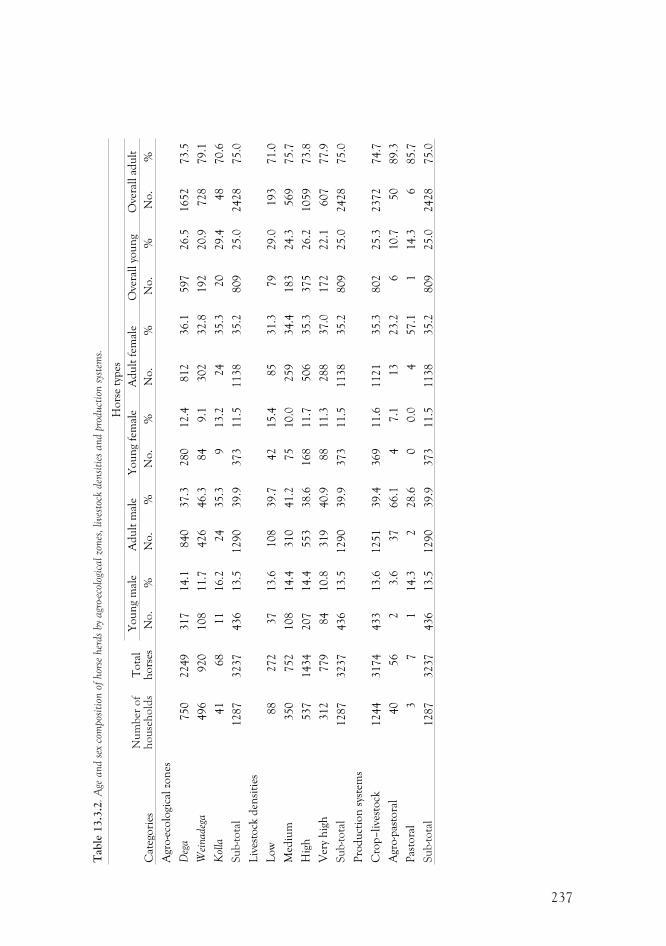
237
Tab
le13.3
.2.A
geand
sex
com
pos
itio
nof
hor
seher
ds
byagr
o-ec
olog
icalzo
nes
,live
stoc
kden
siti
esand
pro
duct
ion
syst
ems.
Cat
ego
ries
Nu
mb
ero
fh
ou
seh
old
sT
ota
lh
ors
es
Ho
rse
typ
es
Yo
un
gm
ale
Ad
ult
mal
eY
ou
ng
fem
ale
Ad
ult
fem
ale
Ove
rall
you
ng
Ove
rall
adu
lt
No
.%
No
.%
No
.%
No
.%
No
.%
No
.%
Agr
o-e
colo
gica
lzo
nes
Deg
a750
2249
317
14.1
840
37.3
280
12.4
812
36.1
597
26.5
1652
73.5
Wei
nadeg
a496
920
108
11.7
426
46.3
84
9.1
302
32.8
192
20.9
728
79.1
Kol
la41
68
11
16.2
24
35.3
913.2
24
35.3
20
29.4
48
70.6
Su
b-to
tal
1287
3237
436
13.5
1290
39.9
373
11.5
1138
35.2
809
25.0
2428
75.0
Liv
esto
ckd
ensi
ties
Lo
w88
272
37
13.6
108
39.7
42
15.4
85
31.3
79
29.0
193
71.0
Med
ium
350
752
108
14.4
310
41.2
75
10.0
259
34.4
183
24.3
569
75.7
Hig
h537
1434
207
14.4
553
38.6
168
11.7
506
35.3
375
26.2
1059
73.8
Ver
yh
igh
312
779
84
10.8
319
40.9
88
11.3
288
37.0
172
22.1
607
77.9
Su
b-to
tal
1287
3237
436
13.5
1290
39.9
373
11.5
1138
35.2
809
25.0
2428
75.0
Pro
du
ctio
nsy
stem
s
Cro
p–li
vest
ock
1244
3174
433
13.6
1251
39.4
369
11.6
1121
35.3
802
25.3
2372
74.7
Agr
o-p
asto
ral
40
56
23.6
37
66.1
47.1
13
23.2
610.7
50
89.3
Pas
tora
l3
71
14.3
228.6
00.0
457.1
114.3
685.7
Su
b-to
tal
1287
3237
436
13.5
1290
39.9
373
11.5
1138
35.2
809
25.0
2428
75.0
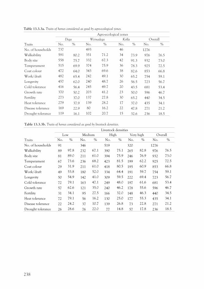
Table 13.3.3a. Traits of horses considered as good by agro-ecological zones.
Traits
Agro-ecological zones
Dega Weinadega Kolla Overall
No. % No. % No. % No. %
No. of households 737 493 46 1276
Walkability 591 80.2 351 71.2 34 73.9 976 76.5
Body size 558 75.7 332 67.3 42 91.3 932 73.0
Temperament 515 69.9 374 75.9 36 78.3 925 72.5
Coat colour 472 64.0 343 69.6 38 82.6 853 66.8
Work/draft 482 65.4 242 49.1 30 65.2 754 59.1
Longevity 457 62.0 240 48.7 26 56.5 723 56.7
Cold tolerance 416 56.4 245 49.7 20 43.5 681 53.4
Growth rate 370 50.2 203 41.2 23 50.0 596 46.7
Fertility 273 37.0 137 27.8 30 65.2 440 34.5
Heat tolerance 279 37.9 139 28.2 17 37.0 435 34.1
Disease tolerance 169 22.9 80 16.2 22 47.8 271 21.2
Drought tolerance 119 16.1 102 20.7 15 32.6 236 18.5
Table 13.3.3b. Traits of horses considered as good by livestock densities.
Traits
Livestock densities
Low Medium High Very high Overall
No. % No. % No. % No. % No. %
No. of households 91 346 519 320 1276
Walkability 89 97.8 232 67.1 390 75.1 265 82.8 976 76.5
Body size 81 89.0 211 61.0 394 75.9 246 76.9 932 73.0
Temperament 67 73.6 236 68.2 423 81.5 199 62.2 925 72.5
Coat colour 29 31.9 211 61.0 418 80.5 195 60.9 853 66.8
Work/draft 49 53.8 180 52.0 334 64.4 191 59.7 754 59.1
Longevity 50 54.9 142 41.0 309 59.5 222 69.4 723 56.7
Cold tolerance 72 79.1 163 47.1 249 48.0 197 61.6 681 53.4
Growth rate 57 62.6 121 35.0 240 46.2 178 55.6 596 46.7
Fertility 31 34.1 95 27.5 166 32.0 148 46.3 440 34.5
Heat tolerance 72 79.1 56 16.2 130 25.0 177 55.3 435 34.1
Disease tolerance 22 24.2 37 10.7 139 26.8 73 22.8 271 21.2
Drought tolerance 26 28.6 76 22.0 77 14.8 57 17.8 236 18.5
238
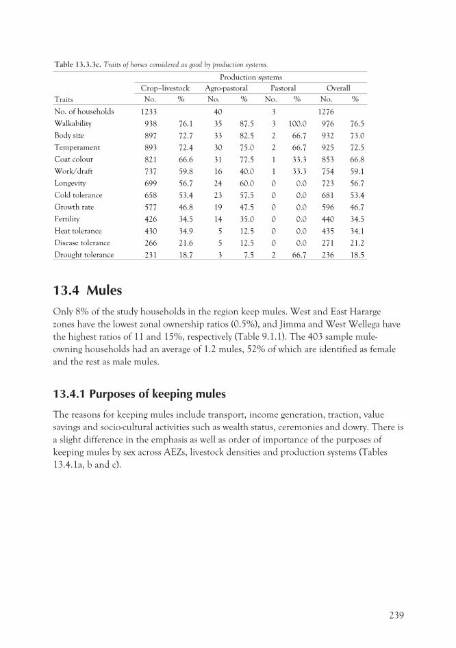
Table 13.3.3c. Traits of horses considered as good by production systems.
Traits
Production systems
Crop–livestock Agro-pastoral Pastoral Overall
No. % No. % No. % No. %
No. of households 1233 40 3 1276
Walkability 938 76.1 35 87.5 3 100.0 976 76.5
Body size 897 72.7 33 82.5 2 66.7 932 73.0
Temperament 893 72.4 30 75.0 2 66.7 925 72.5
Coat colour 821 66.6 31 77.5 1 33.3 853 66.8
Work/draft 737 59.8 16 40.0 1 33.3 754 59.1
Longevity 699 56.7 24 60.0 0 0.0 723 56.7
Cold tolerance 658 53.4 23 57.5 0 0.0 681 53.4
Growth rate 577 46.8 19 47.5 0 0.0 596 46.7
Fertility 426 34.5 14 35.0 0 0.0 440 34.5
Heat tolerance 430 34.9 5 12.5 0 0.0 435 34.1
Disease tolerance 266 21.6 5 12.5 0 0.0 271 21.2
Drought tolerance 231 18.7 3 7.5 2 66.7 236 18.5
13.4 MulesOnly 8% of the study households in the region keep mules. West and East Hararge
zones have the lowest zonal ownership ratios (0.5%), and Jimma and West Wellega have
the highest ratios of 11 and 15%, respectively (Table 9.1.1). The 403 sample mule-
owning households had an average of 1.2 mules, 52% of which are identified as female
and the rest as male mules.
13.4.1 Purposes of keeping mules
The reasons for keeping mules include transport, income generation, traction, value
savings and socio-cultural activities such as wealth status, ceremonies and dowry. There is
a slight difference in the emphasis as well as order of importance of the purposes of
keeping mules by sex across AEZs, livestock densities and production systems (Tables
13.4.1a, b and c).
239
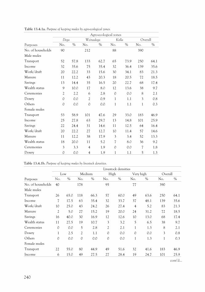
Table 13.4.1a. Purpose of keeping mules by agro-ecological zones.
Purposes
Agro-ecological zones
Dega Weinadega Kolla Overall
No. % No. % No. % No. %
No. of households 90 212 88 390
Male mules
Transport 52 57.8 133 62.7 65 73.9 250 64.1
Income 32 35.6 75 35.4 32 36.4 139 35.6
Work/draft 20 22.2 33 15.6 30 34.1 83 21.3
Manure 11 12.2 43 20.3 18 20.5 72 18.5
Savings 13 14.4 35 16.5 20 22.7 68 17.4
Wealth status 9 10.0 17 8.0 12 13.6 38 9.7
Ceremonies 2 2.2 6 2.8 0 0.0 8 2.1
Dowry 0 0.0 2 0.9 1 1.1 3 0.8
Others 0 0.0 0 0.0 1 1.1 1 0.3
Female mules
Transport 53 58.9 101 47.6 29 33.0 183 46.9
Income 25 27.8 63 29.7 13 14.8 101 25.9
Savings 22 24.4 31 14.6 11 12.5 64 16.4
Work/draft 20 22.2 27 12.7 10 11.4 57 14.6
Manure 11 12.2 38 17.9 3 3.4 52 13.3
Wealth status 18 20.0 11 5.2 7 8.0 36 9.2
Ceremonies 3 3.3 4 1.9 0 0.0 7 1.8
Dowry 0 0.0 4 1.9 1 1.1 5 1.3
Table 13.4.1b. Purpose of keeping mules by livestock densities.
Purposes
Livestock densities
Low Medium High Very high Overall
No. % No. % No. % No. % No. %
No. of households 40 178 95 77 390
Male mules
Transport 26 65.0 118 66.3 57 60.0 49 63.6 250 64.1
Income 7 17.5 63 35.4 32 33.7 37 48.1 139 35.6
Work/draft 10 25.0 43 24.2 26 27.4 4 5.2 83 21.3
Manure 2 5.0 27 15.2 19 20.0 24 31.2 72 18.5
Savings 16 40.0 30 16.9 12 12.6 10 13.0 68 17.4
Wealth status 11 27.5 19 10.7 3 3.2 5 6.5 38 9.7
Ceremonies 0 0.0 5 2.8 2 2.1 1 1.3 8 2.1
Dowry 1 2.5 2 1.1 0 0.0 0 0.0 3 0.8
Others 0 0.0 0 0.0 0 0.0 1 1.3 1 0.3
Female mules
Transport 22 55.0 80 44.9 49 51.6 32 41.6 183 46.9
Income 6 15.0 49 27.5 27 28.4 19 24.7 101 25.9
240
cont’d...
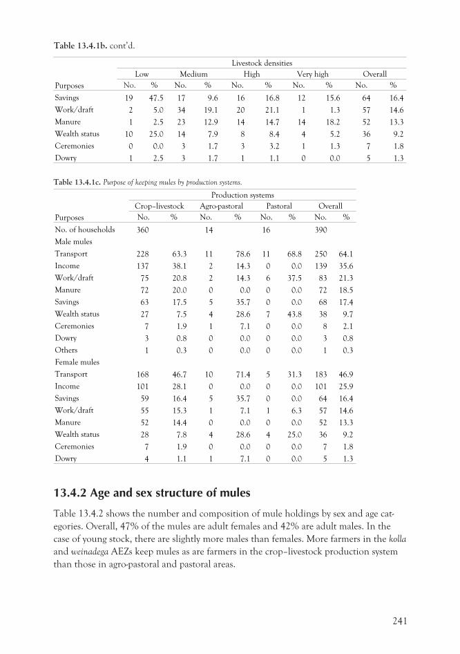
Purposes
Livestock densities
Low Medium High Very high Overall
No. % No. % No. % No. % No. %
Savings 19 47.5 17 9.6 16 16.8 12 15.6 64 16.4
Work/draft 2 5.0 34 19.1 20 21.1 1 1.3 57 14.6
Manure 1 2.5 23 12.9 14 14.7 14 18.2 52 13.3
Wealth status 10 25.0 14 7.9 8 8.4 4 5.2 36 9.2
Ceremonies 0 0.0 3 1.7 3 3.2 1 1.3 7 1.8
Dowry 1 2.5 3 1.7 1 1.1 0 0.0 5 1.3
Table 13.4.1c. Purpose of keeping mules by production systems.
Purposes
Production systems
Crop–livestock Agro-pastoral Pastoral Overall
No. % No. % No. % No. %
No. of households 360 14 16 390
Male mules
Transport 228 63.3 11 78.6 11 68.8 250 64.1
Income 137 38.1 2 14.3 0 0.0 139 35.6
Work/draft 75 20.8 2 14.3 6 37.5 83 21.3
Manure 72 20.0 0 0.0 0 0.0 72 18.5
Savings 63 17.5 5 35.7 0 0.0 68 17.4
Wealth status 27 7.5 4 28.6 7 43.8 38 9.7
Ceremonies 7 1.9 1 7.1 0 0.0 8 2.1
Dowry 3 0.8 0 0.0 0 0.0 3 0.8
Others 1 0.3 0 0.0 0 0.0 1 0.3
Female mules
Transport 168 46.7 10 71.4 5 31.3 183 46.9
Income 101 28.1 0 0.0 0 0.0 101 25.9
Savings 59 16.4 5 35.7 0 0.0 64 16.4
Work/draft 55 15.3 1 7.1 1 6.3 57 14.6
Manure 52 14.4 0 0.0 0 0.0 52 13.3
Wealth status 28 7.8 4 28.6 4 25.0 36 9.2
Ceremonies 7 1.9 0 0.0 0 0.0 7 1.8
Dowry 4 1.1 1 7.1 0 0.0 5 1.3
13.4.2 Age and sex structure of mules
Table 13.4.2 shows the number and composition of mule holdings by sex and age cat-
egories. Overall, 47% of the mules are adult females and 42% are adult males. In the
case of young stock, there are slightly more males than females. More farmers in the kolla
and weinadega AEZs keep mules as are farmers in the crop–livestock production system
than those in agro-pastoral and pastoral areas.
241
Table 13.4.1b. cont’d.
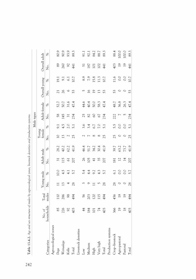
242
Tab
le13.4
.2.
Age
and
sex
stru
cture
ofm
ule
sby
agr
o-ec
olog
icalzo
nes
,live
stoc
kden
siti
esand
pro
duct
ion
syst
ems.
Cat
ego
ries
No
.o
fh
ou
seh
old
sT
ota
lm
ule
s
Mu
lety
pes
Yo
un
gm
ale
Ad
ult
mal
eY
ou
ng
fem
ale
Ad
ult
fem
ale
Ove
rall
you
ng
Ove
rall
adu
lt
No
.%
No
.%
No
.%
No
.%
No
.%
No
.%
Agr
o-e
colo
gica
lzo
nes
Deg
a85
110
11
10.0
31
28.2
10
9.1
58
52.7
21
19.1
89
80.9
Wei
nadeg
a226
286
13
4.5
115
40.2
13
4.5
145
50.7
26
9.1
260
90.9
Kol
la92
98
44.1
61
62.2
22
.031
31.6
66.1
92
93.9
To
tal
403
494
28
5.7
207
41.9
25
5.1
234
47.4
53
10.7
441
89.3
Liv
esto
ckd
ensi
ties
Lo
w44
56
35.4
26
46.4
23.6
25
44.6
58.9
51
91.1
Med
ium
184
203
94.4
105
51.7
73.4
82
40.4
16
7.9
187
92.1
Hig
h101
120
11
9.2
41
34.2
86.7
60
50.0
19
15.8
101
84.2
Ver
yh
igh
74
115
54.3
35
30.4
87.0
67
58.3
13
11.3
102
88.7
To
tal
403
494
28
5.7
207
41.9
25
5.1
234
47.4
53
10.7
441
89.3
Pro
du
ctio
nsy
stem
s
Cro
p–li
vest
ock
366
456
28
6.1
181
39.7
25
5.5
222
48.7
53
11.6
403
88.4
Agr
o-p
asto
ral
19
19
00.0
12
63.2
00.0
736.8
00.0
19
100.0
Pas
tora
l18
19
00.0
14
73.7
00.0
526.3
00
.019
100.0
To
tal
403
494
28
5.7
207
41.9
25
5.1
234
47.4
53
10.7
441
89.3
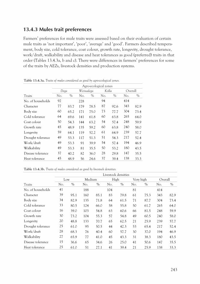
13.4.3 Mules trait preferences
Farmers’ preferences for mule traits were assessed based on their evaluation of certain
mule traits as ‘not important’, ‘poor’, ‘average’ and ‘good’. Farmers described tempera-
ment, body size, cold tolerance, coat colour, growth rate, longevity, drought tolerance,
work/draft, walkability and disease and heat tolerances as good (preferred) traits in that
order (Tables 13.4.3a, b and c). There were differences in farmers’ preferences for some
of the traits by AEZs, livestock densities and production systems.
Table 13.4.3a. Traits of mules considered as good by agro-ecological zones.
Traits
Agro-ecological zones
Dega Weinadega Kolla Overall
No. % No. % No. % No. %
No. of households 92 228 94 414
Character 77 83.7 179 78.5 87 92.6 343 82.9
Body size 60 65.2 171 75.0 73 77.7 304 73.4
Cold tolerance 64 69.6 141 61.8 60 63.8 265 64.0
Coat colour 50 54.3 144 63.2 54 57.4 248 59.9
Growth rate 45 48.9 135 59.2 60 63.8 240 58.0
Longevity 59 64.1 119 52.2 61 64.9 239 57.7
Drought tolerance 49 53.3 117 51.3 51 54.3 217 52.4
Work/draft 49 53.3 91 39.9 54 57.4 194 46.9
Walkability 49 53.3 81 35.5 50 53.2 180 43.5
Disease tolerance 37 40.2 82 36.0 28 29.8 147 35.5
Heat tolerance 45 48.9 56 24.6 37 39.4 138 33.3
Table 13.4.3b. Traits of mules considered as good by livestock densities.
Traits
Livestock densities
Low Medium High Very high Overall
No. % No. % No. % No. % No. %
No. of households 41 188 104 81 414
Character 39 95.1 160 85.1 83 79.8 61 75.3 343 82.9
Body size 34 82.9 135 71.8 64 61.5 71 87.7 304 73.4
Cold tolerance 33 80.5 124 66.0 58 55.8 50 61.7 265 64.0
Coat colour 16 39.0 103 54.8 63 60.6 66 81.5 248 59.9
Growth rate 30 73.2 104 55.3 57 54.8 49 60.5 240 58.0
Longevity 20 48.8 133 70.7 65 62.5 21 25.9 239 57.7
Drought tolerance 25 61.0 95 50.5 44 42.3 53 65.4 217 52.4
Work/draft 28 68.3 76 40.4 60 57.7 30 37.0 194 46.9
Walkability 27 65.9 77 41.0 45 43.3 31 38.3 180 43.5
Disease tolerance 15 36.6 65 34.6 26 25.0 41 50.6 147 35.5
Heat tolerance 25 61.0 51 27.1 41 39.4 21 25.9 138 33.3
243
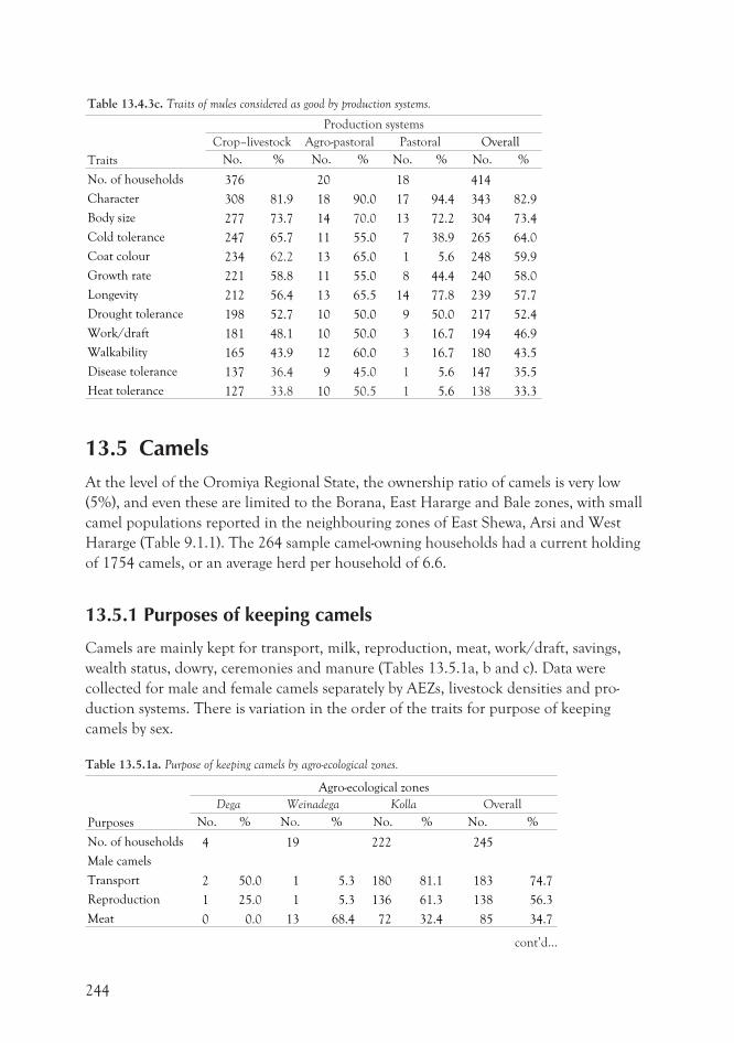
Table 13.4.3c. Traits of mules considered as good by production systems.
Traits
Production systems
Crop–livestock Agro-pastoral Pastoral Overall
No. % No. % No. % No. %
No. of households 376 20 18 414
Character 308 81.9 18 90.0 17 94.4 343 82.9
Body size 277 73.7 14 70.0 13 72.2 304 73.4
Cold tolerance 247 65.7 11 55.0 7 38.9 265 64.0
Coat colour 234 62.2 13 65.0 1 5.6 248 59.9
Growth rate 221 58.8 11 55.0 8 44.4 240 58.0
Longevity 212 56.4 13 65.5 14 77.8 239 57.7
Drought tolerance 198 52.7 10 50.0 9 50.0 217 52.4
Work/draft 181 48.1 10 50.0 3 16.7 194 46.9
Walkability 165 43.9 12 60.0 3 16.7 180 43.5
Disease tolerance 137 36.4 9 45.0 1 5.6 147 35.5
Heat tolerance 127 33.8 10 50.5 1 5.6 138 33.3
13.5 CamelsAt the level of the Oromiya Regional State, the ownership ratio of camels is very low
(5%), and even these are limited to the Borana, East Hararge and Bale zones, with small
camel populations reported in the neighbouring zones of East Shewa, Arsi and West
Hararge (Table 9.1.1). The 264 sample camel-owning households had a current holding
of 1754 camels, or an average herd per household of 6.6.
13.5.1 Purposes of keeping camels
Camels are mainly kept for transport, milk, reproduction, meat, work/draft, savings,
wealth status, dowry, ceremonies and manure (Tables 13.5.1a, b and c). Data were
collected for male and female camels separately by AEZs, livestock densities and pro-
duction systems. There is variation in the order of the traits for purpose of keeping
camels by sex.
Table 13.5.1a. Purpose of keeping camels by agro-ecological zones.
Purposes
Agro-ecological zones
Dega Weinadega Kolla Overall
No. % No. % No. % No. %
No. of households 4 19 222 245
Male camels
Transport 2 50.0 1 5.3 180 81.1 183 74.7
Reproduction 1 25.0 1 5.3 136 61.3 138 56.3
Meat 0 0.0 13 68.4 72 32.4 85 34.7
244
cont’d...
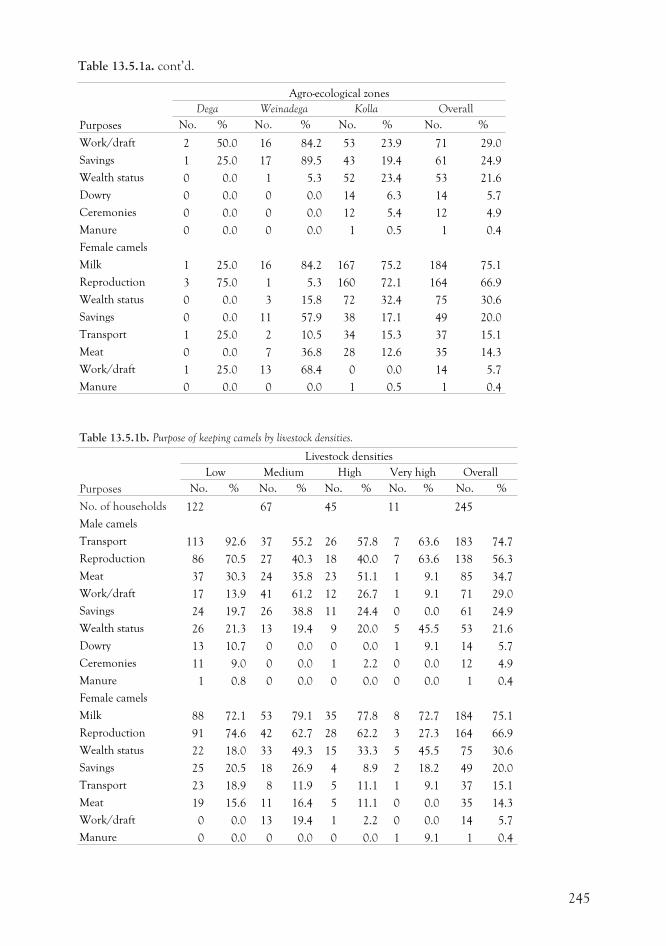
Purposes
Agro-ecological zones
Dega Weinadega Kolla Overall
No. % No. % No. % No. %
Work/draft 2 50.0 16 84.2 53 23.9 71 29.0
Savings 1 25.0 17 89.5 43 19.4 61 24.9
Wealth status 0 0.0 1 5.3 52 23.4 53 21.6
Dowry 0 0.0 0 0.0 14 6.3 14 5.7
Ceremonies 0 0.0 0 0.0 12 5.4 12 4.9
Manure 0 0.0 0 0.0 1 0.5 1 0.4
Female camels
Milk 1 25.0 16 84.2 167 75.2 184 75.1
Reproduction 3 75.0 1 5.3 160 72.1 164 66.9
Wealth status 0 0.0 3 15.8 72 32.4 75 30.6
Savings 0 0.0 11 57.9 38 17.1 49 20.0
Transport 1 25.0 2 10.5 34 15.3 37 15.1
Meat 0 0.0 7 36.8 28 12.6 35 14.3
Work/draft 1 25.0 13 68.4 0 0.0 14 5.7
Manure 0 0.0 0 0.0 1 0.5 1 0.4
Table 13.5.1b. Purpose of keeping camels by livestock densities.
Purposes
Livestock densities
Low Medium High Very high Overall
No. % No. % No. % No. % No. %
No. of households 122 67 45 11 245
Male camels
Transport 113 92.6 37 55.2 26 57.8 7 63.6 183 74.7
Reproduction 86 70.5 27 40.3 18 40.0 7 63.6 138 56.3
Meat 37 30.3 24 35.8 23 51.1 1 9.1 85 34.7
Work/draft 17 13.9 41 61.2 12 26.7 1 9.1 71 29.0
Savings 24 19.7 26 38.8 11 24.4 0 0.0 61 24.9
Wealth status 26 21.3 13 19.4 9 20.0 5 45.5 53 21.6
Dowry 13 10.7 0 0.0 0 0.0 1 9.1 14 5.7
Ceremonies 11 9.0 0 0.0 1 2.2 0 0.0 12 4.9
Manure 1 0.8 0 0.0 0 0.0 0 0.0 1 0.4
Female camels
Milk 88 72.1 53 79.1 35 77.8 8 72.7 184 75.1
Reproduction 91 74.6 42 62.7 28 62.2 3 27.3 164 66.9
Wealth status 22 18.0 33 49.3 15 33.3 5 45.5 75 30.6
Savings 25 20.5 18 26.9 4 8.9 2 18.2 49 20.0
Transport 23 18.9 8 11.9 5 11.1 1 9.1 37 15.1
Meat 19 15.6 11 16.4 5 11.1 0 0.0 35 14.3
Work/draft 0 0.0 13 19.4 1 2.2 0 0.0 14 5.7
Manure 0 0.0 0 0.0 0 0.0 1 9.1 1 0.4
245
Table 13.5.1a. cont’d.
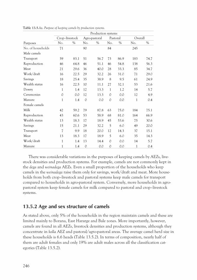
Table 13.5.1c. Purpose of keeping camels by production systems.
Purposes
Production systems
Crop–livestock Agro-pastoral Pastoral Overall
No. % No. % No. % No. %
No. of households 71 90 84 245
Male camels
Transport 59 83.1 51 56.7 73 86.9 183 74.7
Reproduction 46 64.8 46 51.1 46 54.8 138 56.3
Meat 21 29.6 36 40.0 28 33.3 85 34.7
Work/draft 16 22.5 29 32.2 26 31.0 71 29.0
Savings 18 25.4 35 38.9 8 9.5 61 24.9
Wealth status 16 22.5 10 11.1 27 32.1 53 21.6
Dowry 1 1.4 12 13.3 1 1.2 14 5.7
Ceremonies 0 0.0 12 13.3 0 0.0 12 4.9
Manure 1 1.4 0 0.0 0 0.0 1 0.4
Female camels
Milk 42 59.2 79 87.8 63 75.0 184 75.1
Reproduction 43 60.6 53 58.9 68 81.0 164 66.9
Wealth status 13 18.3 17 18.9 45 53.6 75 30.6
Savings 15 21.1 29 32.2 5 6.0 49 20.0
Transport 7 9.9 18 20.0 12 14.3 37 15.1
Meat 13 18.3 17 18.9 5 6.0 35 14.3
Work/draft 1 1.4 13 14.4 0 0.0 14 5.7
Manure 1 1.4 0 0.0 0 0.0 1 0.4
There was considerable variations in the purposes of keeping camels by AEZs, live-
stock densities and production systems. For example, camels are not commonly kept in
the dega and weinadega AEZs. Even a small proportion of the households who keep
camels in the weinadega raise them only for savings, work/draft and meat. More house-
holds from both crop–livestock and pastoral systems keep male camels for transport
compared to households in agro-pastoral system. Conversely, more households in agro-
pastoral system keep female camels for milk compared to pastoral and crop–livestock
systems.
13.5.2 Age and sex structure of camels
As stated above, only 5% of the households in the region maintain camels and these are
limited mainly to Borana, East Hararge and Bale zones. More importantly, however,
camels are found in all AEZs, livestock densities and production systems, although they
concentrate in kolla AEZ and pastoral/agro-pastoral areas. The average camel herd size in
these households is 6.6 heads (Table 13.5.2). In terms of composition, nearly half of
them are adult females and only 19% are adult males across all the classification cat-
egories (Table 13.5.2).
246
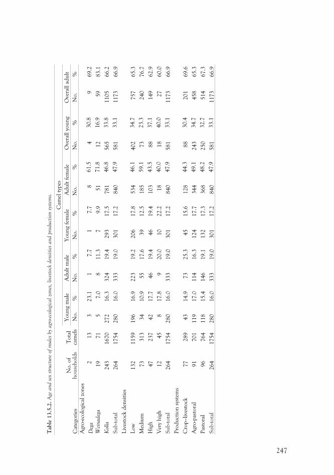
247
Tab
le13.5
.2.
Age
and
sex
stru
cture
ofm
ule
sby
agr
o-ec
olog
icalzo
nes
,live
stoc
kden
siti
esand
pro
duct
ion
syst
ems.
Cat
ego
ries
No
.o
fh
ou
seh
old
sT
ota
lca
mel
s
Cam
elty
pes
Yo
un
gm
ale
Ad
ult
mal
eY
ou
ng
fem
ale
Ad
ult
fem
ale
Ove
rall
you
ng
Ove
rall
adu
lt
No
.%
No
.%
No
.%
No
.%
No
.%
No
.%
Agr
o-e
colo
gica
lzo
nes
Deg
a2
13
323.1
17.7
17.7
861.5
430.8
969.2
Wei
nadeg
a19
71
57.0
811.3
79.9
51
71.8
12
16.9
59
83.1
Kol
la243
1670
272
16.3
324
19.4
293
17.5
781
46.8
565
33.8
1105
66.2
Su
b-to
tal
264
1754
280
16.0
333
19.0
301
17.2
840
47.9
581
33.1
1173
66.9
Liv
esto
ckd
ensi
ties
Lo
w132
1159
196
16.9
223
19.2
206
17.8
534
46.1
402
34.7
757
65.3
Med
ium
73
313
34
10.9
55
17.6
39
12.5
185
59.1
73
23.3
240
76.7
Hig
h47
237
42
17.7
46
19.4
46
19.4
103
43.5
88
37.1
149
62.9
Ver
yh
igh
12
45
817.8
920
.010
22.2
18
40.0
18
40.0
27
60.0
Su
b-to
tal
264
1754
280
16.0
333
19.0
301
17.2
840
47.9
581
33.1
1173
66.9
Pro
du
ctio
nsy
stem
s
Cro
p–li
vest
ock
77
289
43
14.9
73
25.3
45
15.6
128
44.3
88
30.4
201
69.6
Agr
o-p
asto
ral
91
701
119
17.0
114
16.3
124
17.7
344
49.1
243
34.7
458
65.3
Pas
tora
l96
764
118
15.4
146
19.1
132
17.3
368
48.2
250
32.7
514
67.3
Su
b-to
tal
264
1754
280
16.0
333
19.0
301
17.2
840
47.9
581
33.1
1173
66.9
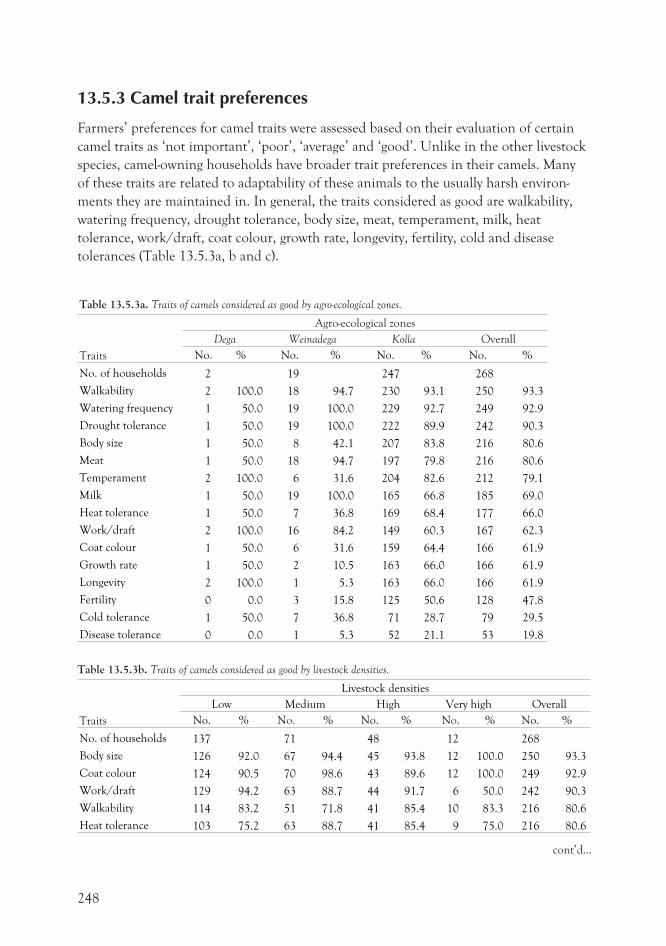
13.5.3 Camel trait preferences
Farmers’ preferences for camel traits were assessed based on their evaluation of certain
camel traits as ‘not important’, ‘poor’, ‘average’ and ‘good’. Unlike in the other livestock
species, camel-owning households have broader trait preferences in their camels. Many
of these traits are related to adaptability of these animals to the usually harsh environ-
ments they are maintained in. In general, the traits considered as good are walkability,
watering frequency, drought tolerance, body size, meat, temperament, milk, heat
tolerance, work/draft, coat colour, growth rate, longevity, fertility, cold and disease
tolerances (Table 13.5.3a, b and c).
Table 13.5.3a. Traits of camels considered as good by agro-ecological zones.
Traits
Agro-ecological zones
Dega Weinadega Kolla Overall
No. % No. % No. % No. %
No. of households 2 19 247 268
Walkability 2 100.0 18 94.7 230 93.1 250 93.3
Watering frequency 1 50.0 19 100.0 229 92.7 249 92.9
Drought tolerance 1 50.0 19 100.0 222 89.9 242 90.3
Body size 1 50.0 8 42.1 207 83.8 216 80.6
Meat 1 50.0 18 94.7 197 79.8 216 80.6
Temperament 2 100.0 6 31.6 204 82.6 212 79.1
Milk 1 50.0 19 100.0 165 66.8 185 69.0
Heat tolerance 1 50.0 7 36.8 169 68.4 177 66.0
Work/draft 2 100.0 16 84.2 149 60.3 167 62.3
Coat colour 1 50.0 6 31.6 159 64.4 166 61.9
Growth rate 1 50.0 2 10.5 163 66.0 166 61.9
Longevity 2 100.0 1 5.3 163 66.0 166 61.9
Fertility 0 0.0 3 15.8 125 50.6 128 47.8
Cold tolerance 1 50.0 7 36.8 71 28.7 79 29.5
Disease tolerance 0 0.0 1 5.3 52 21.1 53 19.8
Table 13.5.3b. Traits of camels considered as good by livestock densities.
Traits
Livestock densities
Low Medium High Very high Overall
No. % No. % No. % No. % No. %
No. of households 137 71 48 12 268
Body size 126 92.0 67 94.4 45 93.8 12 100.0 250 93.3
Coat colour 124 90.5 70 98.6 43 89.6 12 100.0 249 92.9
Work/draft 129 94.2 63 88.7 44 91.7 6 50.0 242 90.3
Walkability 114 83.2 51 71.8 41 85.4 10 83.3 216 80.6
Heat tolerance 103 75.2 63 88.7 41 85.4 9 75.0 216 80.6
248
cont’d...
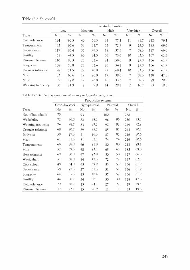
Traits
Livestock densities
Low Medium High Very high Overall
No. % No. % No. % No. % No. %
Cold tolerance 124 90.5 40 56.3 37 77.1 11 91.7 212 79.1
Temperament 83 60.6 58 81.7 35 72.9 9 75.0 185 69.0
Growth rate 117 85.4 35 49.3 18 37.5 7 58.3 177 66.0
Fertility 61 44.5 60 84.5 36 75.0 10 83.3 167 62.3
Disease tolerance 110 80.3 23 32.4 24 50.0 9 75.0 166 61.9
Longevity 108 78.8 23 32.4 26 54.2 9 75.0 166 61.9
Drought tolerance 98 71.5 29 40.8 29 60.4 10 83.3 166 61.9
Meat 83 60.6 19 26.8 19 39.6 7 58.3 128 47.8
Milk 37 27.0 19 26.8 16 33.3 7 58.3 79 29.5
Watering frequency 30 21.9 7 9.9 14 29.2 2 16.7 53 19.8
Table 13.5.3c. Traits of camels considered as good by production systems.
Traits
Production systems
Crop–livestock Agro-pastoral Pastoral Overall
No. % No. % No. % No. %
No. of households 75 93 100 268
Walkability 72 96.0 82 88.2 96 96 250 93.3
Watering frequency 74 98.7 83 89.2 92 92 249 92.9
Drought tolerance 68 90.7 89 95.7 85 85 242 90.3
Body size 58 77.3 71 76.3 87 87 216 80.6
Meat 61 81.3 81 87.1 74 74 216 80.6
Temperament 66 88.0 66 71.0 80 80 212 79.1
Milk 52 69.3 68 73.1 65 65 185 69.0
Heat tolerance 60 80.0 67 72.0 50 50 177 66.0
Work/draft 51 68.0 44 47.3 72 72 167 62.3
Coat colour 48 64.0 65 69.9 53 53 166 61.9
Growth rate 58 77.3 57 61.3 51 51 166 61.9
Longevity 64 85.3 45 48.4 57 57 166 61.9
Fertility 44 58.7 54 58.1 30 30 128 47.8
Cold tolerance 29 38.7 23 24.7 27 27 79 29.5
Disease tolerance 17 22.7 25 26.9 11 11 53 19.8
249
Table 13.5.3b. cont’d.
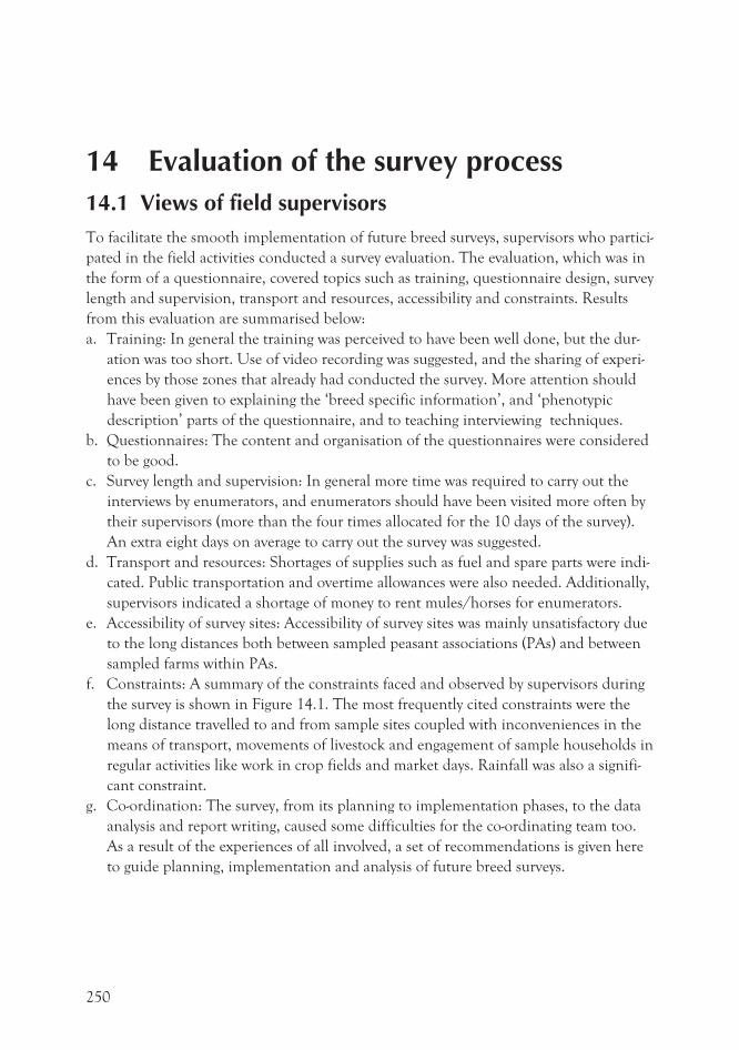
14 Evaluation of the survey process14.1 Views of field supervisorsTo facilitate the smooth implementation of future breed surveys, supervisors who partici-
pated in the field activities conducted a survey evaluation. The evaluation, which was in
the form of a questionnaire, covered topics such as training, questionnaire design, survey
length and supervision, transport and resources, accessibility and constraints. Results
from this evaluation are summarised below:
a. Training: In general the training was perceived to have been well done, but the dur-
ation was too short. Use of video recording was suggested, and the sharing of experi-
ences by those zones that already had conducted the survey. More attention should
have been given to explaining the ‘breed specific information’, and ‘phenotypic
description’ parts of the questionnaire, and to teaching interviewing techniques.
b. Questionnaires: The content and organisation of the questionnaires were considered
to be good.
c. Survey length and supervision: In general more time was required to carry out the
interviews by enumerators, and enumerators should have been visited more often by
their supervisors (more than the four times allocated for the 10 days of the survey).
An extra eight days on average to carry out the survey was suggested.
d. Transport and resources: Shortages of supplies such as fuel and spare parts were indi-
cated. Public transportation and overtime allowances were also needed. Additionally,
supervisors indicated a shortage of money to rent mules/horses for enumerators.
e. Accessibility of survey sites: Accessibility of survey sites was mainly unsatisfactory due
to the long distances both between sampled peasant associations (PAs) and between
sampled farms within PAs.
f. Constraints: A summary of the constraints faced and observed by supervisors during
the survey is shown in Figure 14.1. The most frequently cited constraints were the
long distance travelled to and from sample sites coupled with inconveniences in the
means of transport, movements of livestock and engagement of sample households in
regular activities like work in crop fields and market days. Rainfall was also a signifi-
cant constraint.
g. Co-ordination: The survey, from its planning to implementation phases, to the data
analysis and report writing, caused some difficulties for the co-ordinating team too.
As a result of the experiences of all involved, a set of recommendations is given here
to guide planning, implementation and analysis of future breed surveys.
250
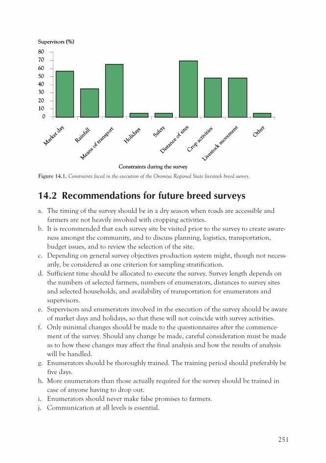
14.2 Recommendations for future breed surveysa. The timing of the survey should be in a dry season when roads are accessible and
farmers are not heavily involved with cropping activities.
b. It is recommended that each survey site be visited prior to the survey to create aware-
ness amongst the community, and to discuss planning, logistics, transportation,
budget issues, and to review the selection of the site.
c. Depending on general survey objectives production system might, though not necess-
arily, be considered as one criterion for sampling stratification.
d. Sufficient time should be allocated to execute the survey. Survey length depends on
the numbers of selected farmers, numbers of enumerators, distances to survey sites
and selected households, and availability of transportation for enumerators and
supervisors.
e. Supervisors and enumerators involved in the execution of the survey should be aware
of market days and holidays, so that these will not coincide with survey activities.
f. Only minimal changes should be made to the questionnaires after the commence-
ment of the survey. Should any change be made, careful consideration must be made
as to how these changes may affect the final analysis and how the results of analysis
will be handled.
g. Enumerators should be thoroughly trained. The training period should preferably be
five days.
h. More enumerators than those actually required for the survey should be trained in
case of anyone having to drop out.
i. Enumerators should never make false promises to farmers.
j. Communication at all levels is essential.
251
0
10
20
30
40
50
60
70
80
Mar
ket da
y
Rainfa
ll
Mea
ns oftran
spor
t
Hol
iday
sSa
fety
Dist
ance
ofsit
es
Cro
pac
tiviti
es
Lives
tock
mov
emen
t
Oth
er
Constraints during the survey
Supervisors (%)
0
10
20
30
40
50
60
70
80
Mar
ket da
y
Rainfa
ll
Mea
ns oftran
spor
t
Hol
iday
sSa
fety
Dist
ance
ofsit
es
Cro
pac
tiviti
es
Lives
tock
mov
emen
t
Oth
er
Constraints during the survey
Supervisors (%)
Figure 14.1. Constraints faced in the execution of the Oromiya Regional State livestock breed survey.
15 ConclusionA primary objective of the survey has been achieved in providing a wide range of base-
line data on livestock production, mainly on cattle, sheep and goats (primary species)
and on chickens, donkeys, horses, mules and camels (secondary species) in the Oromiya
Regional State of Ethiopia. The results demonstrate the diversity in characteristics, man-
agement and use of animal genetic resources and the constraints faced in handling them
across administrative zones, agro-ecological zones, livestock densities and production
systems. Production system was not used as one of the stratification factors in the survey
as the aim was to get an overall picture of the average features of livestock production
across the region. In follow-up surveys, however, it might be useful to stratify for pro-
duction system if it is considered important to quantify these differences better.
Unfortunately, the survey did not lead to a straightforward characterisation of differ-
ent livestock breeds. This was primarily due to the nature of the data collected in which
farmers described their livestock in different ways. The survey also revealed a long list of
breed groups, which were identified by farmers as crosses between the more distinct
breed types. Many of these crossbreds are deliberately produced in an effort to combine
desirable attributes from the different breeds. This has also meant that the sample sizes
of animals from each of the breed type from which measurements (breed descriptors)
were taken were too small for extensive statistical analysis. This operational problem was
not foreseen. There has also been time constraint. As described in Chapter 9.4, however,
a preliminary attempt has been made to identify and test an appropriate statistical pro-
cedure for the data. The procedure, known as, multivariate cluster analysis, is success-
fully demonstrated on a subset of the data (cattle from Borana Zone) and the results are
promising. This procedure has also shown that multivariate techniques can be used for
on-farm breed characterisation work by classifying the observations on individual
animals into well-defined breed types/strains. It is hoped to investigate this technique
further and provide the region with general information on breed types to supplement
the tables provided herein. Clustering based on phenotypic data should, however, be
followed up with molecular genetic analysis of the breed types to increase the accuracy of
identification as well as characterisation of the breed types. Therefore, such multivariate
techniques can help formulating hypotheses, which can be tested using detailed genetic
studies.
The planning of the survey relied on many decisions about many issues being made
within a comparatively short period of time. These decisions on questionnaire and
sampling frame design, organisation of pre-surveys and enumerator training, organis-
ation of manpower, distribution of the budget and other logistics had to take into
account the administrative infrastructure of the region, the distributions of the different
agro-ecological zones, and the seasonal constraints in implementing the survey. Never-
theless, the project team remained dedicated to the task and communicated well with
252
supervisors in the field. This led, in general, to a good result. However, there were some
inconsistencies in the way that the survey was implemented in each zone. This could
have improved through better co-ordination of the survey by pre-visits to each zone and
clearer realisation of how budgetary arrangements could best be handled. The implemen-
tation of the survey tended to be a little rushed and more time to cover the sample house-
holds should be allowed on another occasion. A key lesson that has been learnt through
the execution of this survey, however, is that one should not underestimate the length of
time needed for data entry and analysis. This was grossly underestimated in this survey.
Hopefully, the results of the survey will contribute to future planning of livestock
development and conservation works in the Oromiya Regional State within the different
administrative and agro-ecological zones and for different production systems, and will
help to understand the constraints that need to be tackled to encourage successful live-
stock farming. One could now decide to target activities at the level of administrative
zones, agro-ecological zones, livestock density categories or at the production systems
level. Alternatively, one could decide to target activities directly at breed types. It is,
therefore, up to the livestock experts or the policy makers concerned with livestock devel-
opment and conservation, to decide how to use this information for planning of live-
stock development and conservation activities. Of course, further analyses are needed to
extract additional information on the distributions, performance and perceived attri-
butes of different breed types to help in the design of breeding strategies. As indicated at
the beginning of this report, the amount of data collected from this survey is substantial
and can be analysed in different ways to address different questions. It is a database,
which should be maintained and updated with regular surveys. The database is to be
maintained by the Oromiya Agricultural Development Bureau (OADB) as well as the
Oromiya Agricultural Research Institute (OARI). Hopefully, easy access to this report
will allow different users to undertake investigations of their own so that the database
can be exploited to the full.
253