Embed Size (px)
Citation preview
DESIGN OF A REAL-TIME SCANNING ELECTRICAL MOBILITY
SPECTROMETER AND ITS APPLICATION IN STUDY OF NANOPARTICLE
AEROSOL GENERATION
A Thesis
by
GAGAN SINGH
Submitted to the Office of Graduate Studies of Texas A&M University
in partial fulfillment of the requirements for the degree of
MASTER OF SCIENCE
May 2010
Major Subject: Mechanical Engineering
DESIGN OF A REAL-TIME SCANNING ELECTRICAL MOBILITY
SPECTROMETER AND ITS APPLICATION IN STUDY OF NANOPARTICLE
AEROSOL GENERATION
A Thesis
by
GAGAN SINGH
Submitted to the Office of Graduate Studies of Texas A&M University
in partial fulfillment of the requirements for the degree of
MASTER OF SCIENCE
Approved by:
Chair of Committee, Bing Guo
Committee Members, Renyi Zhang Eric Petersen Head of Department, Dennis O’Neal
May 2010
Major Subject: Mechanical Engineering
iii
ABSTRACT
Design of a Real-Time Scanning Electrical Mobility Spectrometer and Its Application in
Study of Nanoparticle Aerosol Generation. (May 2010)
Gagan Singh, B.S., Texas A&M University
Chair of Advisory Committee: Dr. Bing Guo
A real-time, mobile Scanning Electrical Mobility Spectrometer (SEMS) was designed
using a Condensation Particle Counter (CPC) and Differential Mobility Analyzer
(DMA) to measure the size distribution of nanoparticles. The SEMS was calibrated
using monodisperse Polystyrene Latex (PSL) particles, and was then applied to study the
size distribution of TiO2 nanoparticle aerosols generated by spray drying water
suspensions of the nanoparticles. The nanoparticle aerosol size distribution, the effect of
surfactant, and the effect of residual solvent droplets were determined.
The SEMS system was designed by integrating the Electrical System, the Fluid
Flow System, and the SEMS Software. It was calibrated using aerosolized Polystyrene
Latex (PSL) spheres with nominal diameters of 99 nm and 204 nm. TiO2 nanoparticle
aerosols were generated by atomizing water suspensions of TiO2 nanoparticles using a
Collison nebulizer. Size distribution of the TiO2 aerosol was measured by the SEMS, as
well as by TEM. Furthermore, the effect of surfactant, Tween 20 at four different
concentrations between 0.01mM and 0.80mM, and stability of aerosol concentration
with time were studied. It was hypothesized that residual particles in DI water observed
iv
during the calibration process were a mixture of impurities in water and unevaporated
droplets. Solid impurities were captured on TEM grids using a point-to-plane
Electrostatic Precipitator (ESP) and analyzed by Energy Dispersive Spectroscopy (EDS)
while the contribution of unevaporated liquid droplets to residual particles was
confirmed by size distribution measurements of aerosolized DI water in different
humidity conditions.
The calibration indicated that the mode diameter was found to be at 92.5nm by
TEM and 95.8nm by the SEMS for 99nm nominal diameter particles, a difference of
3.6%. Similarly, the mode diameter for 204nm nominal diameter particles was found to
be 194.9nm by TEM and 191nm by SEMS, a difference of 2.0%. Measurements by
SEMS for TiO2 aerosol generated by Collison nebulizer indicated the mode diameters of
3mM, 6mM, and 9mM concentrations of TiO2 suspension to be 197.5nm, 200.0nm and
195.2nm respectively. On the other hand, the mode diameter was found to be
approximately 95nm from TEM analysis of TiO2 powder. Additionally, concentration of
particles generated decreased with time. Dynamic Light Scattering (DLS) measurements
indicated agglomeration of particles in the suspension. Furthermore, the emulation of
single particle distribution was not possible even after using Tween 20 in concentrations
between 0.01mM and 0.80mM. From the study of residual particles in DI water, it was
found that residual particles observed during the aerosolization of suspensions of DI
water were composed of impurities present in DI water and unevaporated droplets of DI
water. Although it was possible to observe solid residual particles on the TEM grid, EDS
was not able to determine the chemical composition of these particles.
v
ACKNOWLEDGEMENTS
I would like to thank my committee chair, Dr. Bing Guo, for his valuable support and
guidance throughout the course of this research. I would also like to thank Dr. Eric
Petersen and Dr. Renyi Zhang for their recommendations and consideration as
committee members.
I am very grateful to Alexei Khalizov for sharing his expertise in the design of
SEMS system, Wonjoong Hwan for his help with TEM analysis and Andrew Sharp for
sharing his programming knowledge to create the SEMS software.
Finally, I would like to extend my gratitude to my parents for their
encouragement and support throughout my time here at Texas A&M University.
vi
TABLE OF CONTENTS
Page
ABSTRACT .............................................................................................................. iii
ACKNOWLEDGEMENTS ...................................................................................... v
TABLE OF CONTENTS .......................................................................................... vi
LIST OF FIGURES ................................................................................................... viii
LIST OF TABLES .................................................................................................... x
1. INTRODUCTION ............................................................................................... 1 2. SCANNING ELECTRICAL MOBILITY SPECTROMETER – DESIGN
AND CALIBRATION ........................................................................................ 3 2.1 General Operating Principles ............................................................... 3 2.1.1 Theory ...................................................................................... 3
2.1.2 General Design (Hardware Description) .................................. 11
2.1.3 SEMS Software ........................................................................ 18
2.2 Calibration ............................................................................................ 27 2.2.1 Experimental ............................................................................ 27
2.2.2 Results and Conclusions ........................................................... 33
3. A STUDY OF GENERATION OF TITANIUM DIOXIDE PARTICLES USING A COLLISON NEBULIZER ................................................................. 39 3.1 Introduction .......................................................................................... 39 3.2 Theory/Model ....................................................................................... 40 3.3 Experimental ........................................................................................ 41
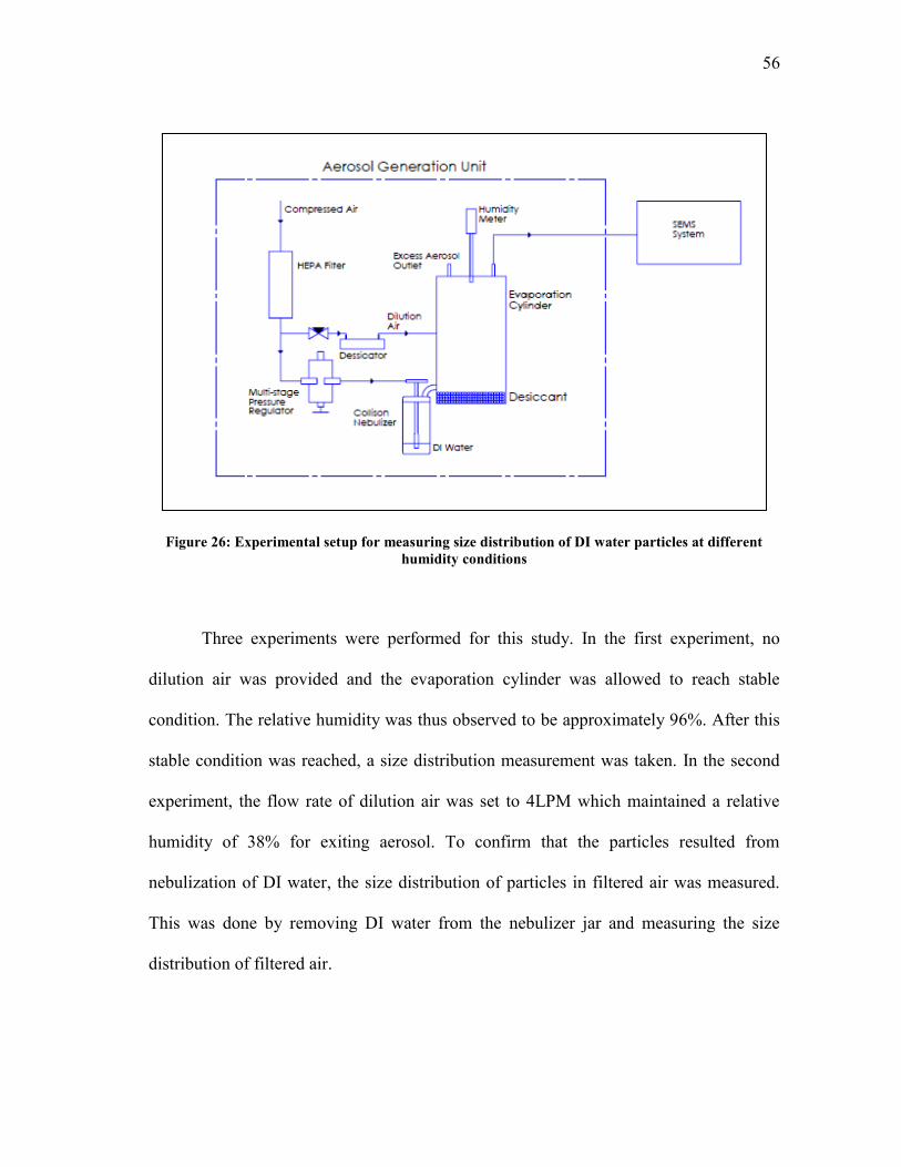
3.4 Results and Conclusions ....................................................................... 44 4. STUDY OF BACKGROUND PARTICLES IN AEROSOLIZED DE-IONIZED WATER ....................................................................................... 53 4.1 Background .......................................................................................... 53 4.2 Hypothesis/Model ................................................................................ 54 4.3 Experimental ........................................................................................ 55 4.4 Results and Conclusions ....................................................................... 58
vii
Page
5. SUMMARY ........................................................................................................ 62
REFERENCES .......................................................................................................... 64
APPENDIX ............................................................................................................... 67
VITA ......................................................................................................................... 69
viii
LIST OF FIGURES
Page
Figure 1: Schematic of Scanning Electrical Mobility Spectrometer ......................... 4
Figure 2: Particle Trajectories in Differential Mobility Analyzer (Wang and Flagan 1990) .......................................................................................................... 7 Figure 3: SEMS electrical system ............................................................................. 12
Figure 4: Interface between HVS and CPC .............................................................. 13
Figure 5: Interface between HVS and DMA ............................................................. 13
Figure 6: Schematic of the Fluid Flow System for the SEMS system ...................... 15
Figure 7: Software model for the SEMS system ....................................................... 18
Figure 8: SEMS algorithm flowchart showing the program design to obtain particle size distribution of aerosols ....................................................................... 21 Figure 9: CPC 3772 detection efficiency with respect to particle diameter (Shown here with permission from TSI Inc.) .......................................................... 26 Figure 10: Example of graphical representation of particle size distribution by SEMS. ..................................................................................................... 27 Figure 11: Setup for pressure testing the classifier for leakage ................................ 30
Figure 12: Apparatus setup for SEMS Calibration ................................................... 32
Figure 13: Comparison of theoretical or programming voltage provided to HVS and its high voltage response. ................................................................. 34 Figure 14: TEM image of 99nm PSL particles ......................................................... 34
Figure 15: TEM image of 204nm PSL particles ....................................................... 35
Figure 16: Particle size distribution of 99nm PSL particles as measured by SEMS system ...................................................................................................... 36
ix
Page
Figure 17: Particle size distribution of 204nm PSL particles as measured by SEMS system .......................................................................................... 37 Figure 18: Model for study of aerosol generated by Collison nebulizer. .................. 41
Figure 19: Apparatus setup for measuring particle size distribution of Titanium dioxide particles generated by a Collison nebulizer ................................ 42 Figure 20: Particle size distribution of various concentrations of Titanium dioxide suspensions .............................................................................................. 46 Figure 21: Size distribution of 9.0mM Titanium dioxide suspension for 6 trials taken at different times during Collison nebulizer run ............................ 46 Figure 22: Size distribution measurement of 1mM Titanium dioxide suspension found using Dynamic Light Scattering (DLS) technique ........................ 48 Figure 23: Agglomeration observed between size distribution measurements of 9.0mM Titanium dioxide suspension during nebulization by an increase in mode diameter for consecutive measurements ................................... 49 Figure 24: Size distribution of single particles in flame synthesized Titanium dioxide powder found by TEM analysis ................................................. 49 Figure 25: Size distribution of nebulized 6.0mM TiO2 + Tween-20 suspension with varying concentrations of Tween 20 ............................................... 50 Figure 26: Experimental setup for measuring size distribution of DI water particles at different humidity conditions .............................................................. 56 Figure 27: Schematic of apparatus setup for collection of particles in de-ionized water ........................................................................................................ 57 Figure 28: Particle size distribution of residual particles at different humidity conditions ................................................................................................ 59 Figure 29: TEM image of residual particles in DI water collected using an Electrostatic Precipitator ......................................................................... 60 Figure 30: Quantitative analysis of DI water particles with EDS technique ............ 60
x
LIST OF TABLES
Page
Table 1: Coefficients for Fuchs’ equation………………………………………... 25
Table 2: An explanation of additional peaks observed in size distribution of 99nm and 204nm PSL particles……………………………………………...... 38 Table 3: Mode diameters of particle size distribution of TiO2 suspension with varying concentrations of Tween 20……………………………………. 51
1
1. INTRODUCTION
Size is perhaps the most fundamental parameter describing an aerosol. Particles in
aerosols can be many orders of magnitude, from just a few nanometers to around
100 micrometer (Baron and Willeke 2001). Physical and chemical properties of
aerosols depend on their size distribution and thus, it is an essential feature of
aerosol study. A number of researchers analyze size distribution of aerosols to reach
valuable conclusions. Size distribution measurement is an important analytical tool in a
number of fields such as atmospheric sciences, combustion studies, flame synthesis of
particles and in the area of health and safety. For example, analysis of soot nanoparticles
is done by characterizing combustion soot by studying its size distribution (Zhao et al.
2003). Another example is the measurement of modes and geometric means of particles
near a major highway to determine exposure to ultrafine particles (Zhu et al. 2002).
Various tools can be used to determine size distribution of aerosols. These
include the Electrical Aerosol Analyzer (EAA), Scanning Electrical Mobility
Spectrometer (SEMS), Optical Particle Counters, Cascade Impactors and Aerodynamic
Particle Sizers (APS). Among these, the SEMS is perhaps the most widely used
instrument for size distribution measurements. A differential mobility analyzer (DMA)
classifies particles into a narrow range of mobility which are then counted by a
condensation particle counter (CPC). The first differential mobility analyzer was
developed by Erikson (1921) for understanding the evolution of mobility of small ions.
____________ This thesis follows the style of Aerosol Science and Technology.
2
Even though this instrument could provide differential measurements of ion mobility
with high resolution, lack of a suitable detector limited its use. Development of
continuous flow condensation particle counter by Bricard and coworkers provided the
required sensitivity and time response for particle size distribution measurements
(Flagan 1998). The SEMS is commercially available as the Scanning Mobility Particle
Sizer (SMPS) system and is offered by TSI, Inc.
Major advantages of the SEMS system include its ease of transportation, low
power consumption, and high resolution in measurement of particles. The SEMS also
has an important advantage over the stepping mode of operation. Many systems such as
smog chambers, combustion sources and industrial processes change composition
rapidly. The scanning mode is appropriate for determining particle size distribution in
these cases as significant noise is observed in the signals in stepping mode (Wang and
Flagan 1990). Typical time required for completing a particle size distribution
measurement in stepping mode varies from 10 minutes to an hour or more.
Concentrations for over 100 mobilities can be measured using the scanning mode in 20
to 30s as found by Wang and Flagan. In this paper, the design and calibration of a SEMS
system is described. This not only offers a cheaper alternative to the otherwise expensive
commercially available systems but also can be customized to the needs of the
researcher. Finally, the SEMS system has been applied to study the generation of
Titanium dioxide nanoparticles using a Collison nebulizer and residual particles in the
aerosolized De-ionized water. These studies are also described in the thesis.
3
2. SCANNING ELECTRICAL MOBILITY SPECTROMETER-DESIGN AND
CALIBRATION
2.1 General Operating Principles
2.1.1 Theory
The Scanning Electrical Mobility Spectrometer (SEMS) operates by classifying particles
based on electrical mobility and counting the particles using a detector. In the system,
the aerosol first passes through a bipolar charger which creates negative and positive
charges on particles and reaches a Fuchs’ equilibrium charge distribution. The aerosol
particles then pass through a Differential Mobility Analyzer (DMA) in which they are
separated according to their electrical mobility. The SEMS operating principle can be
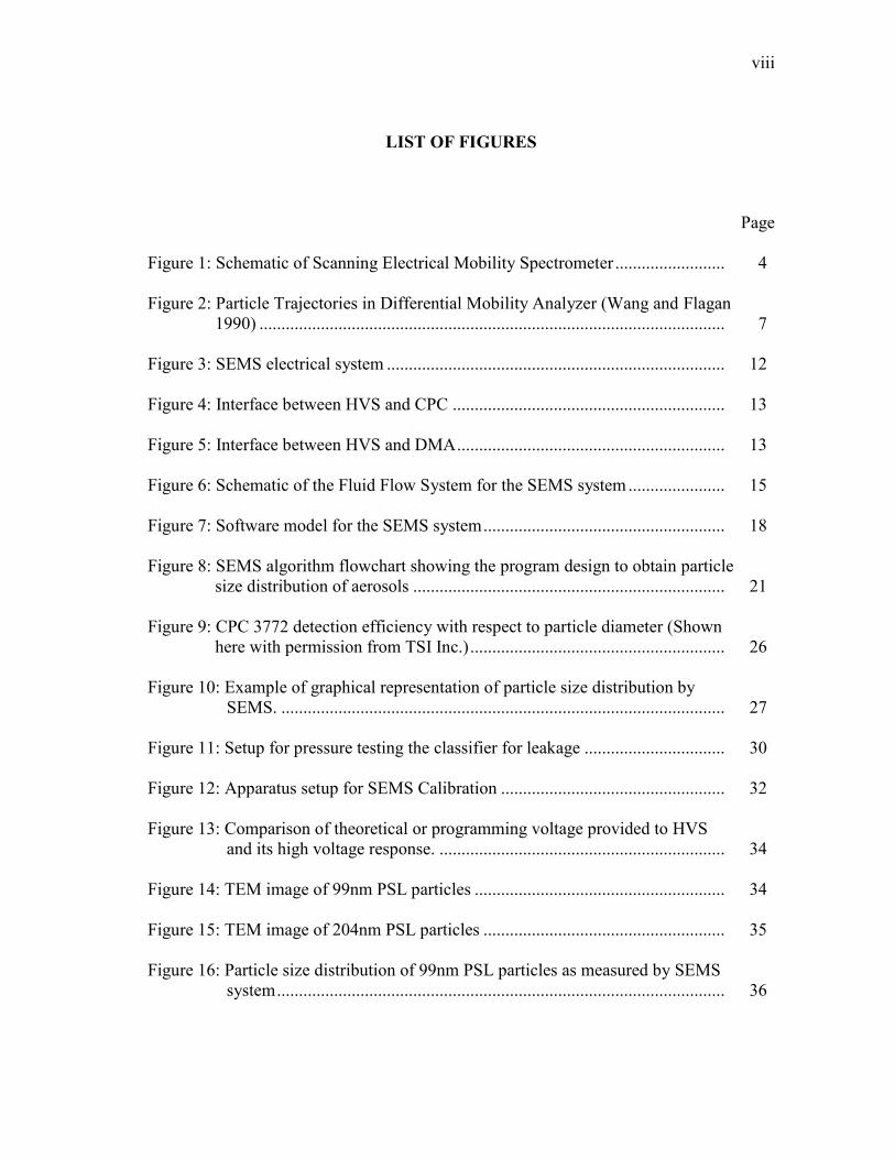
explained with the help of the DMA schematic in Figure 1.
The DMA consists of the inner and outer electrodes in the form of concentric
cylinders. A high voltage is applied to the inner electrode which attracts particles of the
opposite charge. The outer electrode is kept at ground potential and particles having the
same polarity of charge as the inner electrode are deposited on the wall. Neutral particles
exit along with excess air. HEPA-filtered sheath air is introduced in the DMA and flows
in the annular space between the electrodes. The flows for both the sheath air and
aerosol flow are controlled upstream of the DMA. Particles in a narrow range of
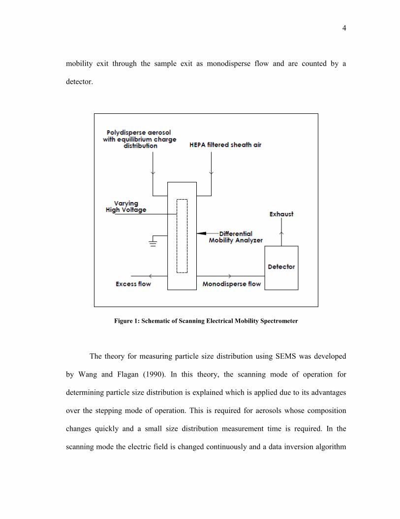
4
mobility exit through the sample exit as monodisperse flow and are counted by a
detector.
Figure 1: Schematic of Scanning Electrical Mobility Spectrometer
The theory for measuring particle size distribution using SEMS was developed
by Wang and Flagan (1990). In this theory, the scanning mode of operation for
determining particle size distribution is explained which is applied due to its advantages
over the stepping mode of operation. This is required for aerosols whose composition
changes quickly and a small size distribution measurement time is required. In the
scanning mode the electric field is changed continuously and a data inversion algorithm
5
produces results of size distribution for the aerosol. For scanning mode of operation,
continuously varying electric field at the center rod is given as
)(11 tEE [1]
It is assumed that the time during which the electric field changes is much longer
than the aerodynamic relaxation time of particles and hence inertial effects can be
neglected. Particles reach the extraction slot of the DMA from the aerosol inlet after a
fluid residence time tf. It is assumed that the particles would reside in the analyzer
column for the same time as the fluid. After a delay of td from the time particles are
extracted from the DMA, particles reach the detector. After time tf+td, from the start of
scanning process the first particle would reach the detector and all following particles
would have different mobility. The instrument response functions for determining the
size distribution of aerosols are derived in the following paragraphs.
Radial migration of charged particles in the DMA with a continuously varying
electric field can be described by
r
rtEZ
dt
drp
11 )(
[2]
where Zp is the electrical mobility of particle, and r is the radial position of the particle
with respect to the center rod. A schematic showing trajectories of particles in the DMA
is shown in Figure 2. Radial position of the particles that entered the analyzer at tin, after
a time t inside the analyzer column can be found by integrating Equation [2].
tt
t
pinin
in
in
dttErZrttr ')'(2)( 11
22
[3]
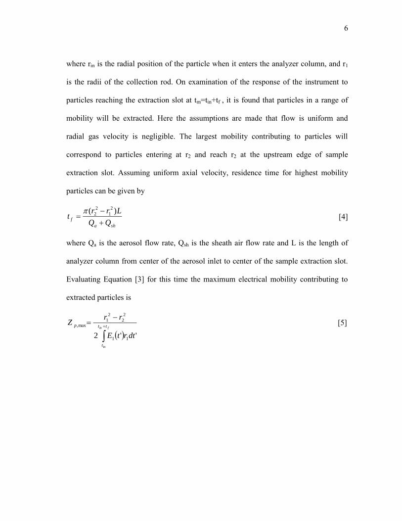
6
where rin is the radial position of the particle when it enters the analyzer column, and r1
is the radii of the collection rod. On examination of the response of the instrument to
particles reaching the extraction slot at tm=tin+tf , it is found that particles in a range of
mobility will be extracted. Here the assumptions are made that flow is uniform and
radial gas velocity is negligible. The largest mobility contributing to particles will
correspond to particles entering at r2 and reach r2 at the upstream edge of sample
extraction slot. Assuming uniform axial velocity, residence time for highest mobility
particles can be given by
sha
fQQ
Lrrt
)( 2
1
2
2
[4]
where Qa is the aerosol flow rate, Qsh is the sheath air flow rate and L is the length of
analyzer column from center of the aerosol inlet to center of the sample extraction slot.
Evaluating Equation [3] for this time the maximum electrical mobility contributing to
extracted particles is
fin
in
tt
t
p
dtrtE
rrZ
''2 11
2
2
2
1max,
[5]
7
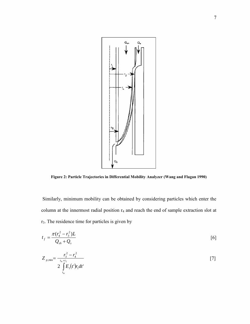
Figure 2: Particle Trajectories in Differential Mobility Analyzer (Wang and Flagan 1990) Similarly, minimum mobility can be obtained by considering particles which enter the
column at the innermost radial position r4 and reach the end of sample extraction slot at
r3. The residence time for particles is given by
ssh
fQQ
Lrrt
)( 2
3
2
4
[6]
fin
in
tt
t
p
dtrtE
rrZ
''2 11
2
4
2
3min,
[7]
8
Only a fraction of particles entering the DMA between this mobility range will
be extracted. These particles will reach the sample extraction slot at r1<r≤r3. Particles
with mobility greater than Zp,min will contribute to sample flow only if they are within a
critical radial position rc. Particles following this critical trajectory must reach r3 in
sash
cf
QfQQ
Lrrt
)( 2
3
2
[8]
where
)(
)(22
2
2
4
2
a
c
rr
rrf
[9]
where f is the fraction of aerosol flow entering the sample extraction slot with r<rc.
Rearranging Equation [8] and using Equation [3]
a
shsm
Q
QQtKf
)(
[10]
where
)(2)( 11 mpm tELZrtK [11]
and
m
fm
t
ttf
m dttEt
tE ')'(1
)( 11
[12]
A similar analysis for particles with mobility smaller than Zp,max gives
a
sham
Q
QQtKf
)(
[13]
In case of a smaller sample flow than the aerosol flow, the fraction extracted cannot be
larger than
9
a
s
Q
Qf
[14]
For any mobility Zp, the fraction of particles extracted will be
1,,
)(,
)(min,0max
a
s
a
sham
a
shsm
Q
Q
Q
QQtK
Q
QQtK
[15]
As the field is varying continuously, critical trajectories depend upon the time
particles enter the analyzer column. To eliminate this dependence an exponentially
changing electric field is chosen.
tetE )(1 [16]
Substituting in Equation [3], the particle trajectory is
)1()(2)()( 1
22 tt
pinin eerZtrttr in
[17]
And the mobility parameter for this ramping function is
mf tt
f
pm eet
LZrtK
12)( 1
[18]
It can be seen here that an exponential ramp ensures the dependence of critical
trajectories and transfer function only on K(tm). In the SEMS, the electric field is varied
continuously and the particles extracted are monitored using a Condensation Particle
Counter (CPC). To reach the detector, the particles need to flow through the plumbing,
which takes an additional delay td. Counts made by the CPC need to be taken for a finite
time in order to obtain statistically relevant results. This counting time is tc.
The relevant transfer function is obtained by averaging over the counting time.
10
cm
m
tt
t
p
c
dttZt
),(1
[19]
Fraction of particles of mobility Zp extracted through the analyzer column is described
by the transfer function. The mobility of particles is
p
cp
D
neCZ
3
[20]
where n is the number of elementary charges, e is the elementary charge, µ is the gas
viscosity, Cc is the Cunningham slip correction factor and Dp is the particle diameter.
Particles acquire an equilibrium charge distribution when they pass through a bipolar
charger. The probability for a particle of diameter Dp acquiring a charge i can be
predicted by Wiedensohler (1988) which is an approximation of Fuchs (1963) model and
is given by
5
0
log)(
10),(k
k
pk
nm
Dia
p iD [21]
where ai(N) are the coefficients for the equation and N is the number of elementary
charges on particles. The detector response to particles of diameter Dp and charge i is
given by s(Dp,i). The instrument response is the weighted integral over counting time tc,
thus at time t=tm+td+tc, the response obtained is
0
),,()()( pcmpp dDttDDntS
[22]
where the system response function is
i
cmppppcmp ttiDZiDiDsttD ),),,((),(),(),,(
[23]
11
A response is obtained after every interval tc at time tj which can be described as
cdj jttt [24]
where j=1,2,………………N.
From these measurement Sj , n(Dp) is to be found.
2.1.2 General Design (Hardware Description)
The SEMS system can be separated into two sub-systems. These are the electrical
system and the fluid flow system. For each system the design, operation and components
are described in the following sections.
Electrical System
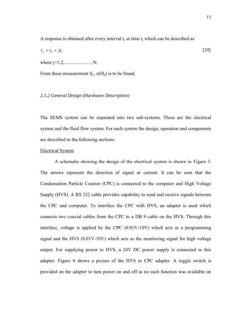
A schematic showing the design of the electrical system is shown in Figure 3.
The arrows represent the direction of signal or current. It can be seen that the
Condensation Particle Counter (CPC) is connected to the computer and High Voltage
Supply (HVS). A RS 232 cable provides capability to send and receive signals between
the CPC and computer. To interface the CPC with HVS, an adapter is used which
connects two coaxial cables from the CPC to a DB 9 cable on the HVS. Through this
interface, voltage is applied by the CPC (0.01V-10V) which acts as a programming
signal and the HVS (0.01V-10V) which acts as the monitoring signal for high voltage
output. For supplying power to HVS, a 24V DC power supply is connected to this
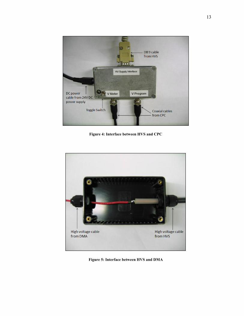
adapter. Figure 4 shows a picture of the HVS to CPC adapter. A toggle switch is
provided on the adapter to turn power on and off as no such function was available on
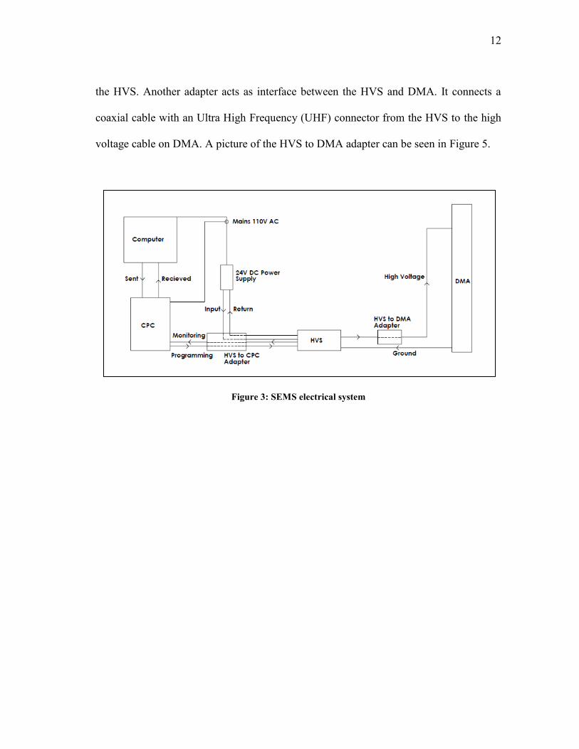
12
the HVS. Another adapter acts as interface between the HVS and DMA. It connects a
coaxial cable with an Ultra High Frequency (UHF) connector from the HVS to the high
voltage cable on DMA. A picture of the HVS to DMA adapter can be seen in Figure 5.
Figure 3: SEMS electrical system
13
Figure 4: Interface between HVS and CPC
Figure 5: Interface between HVS and DMA
14
To describe the operation of SEMS electrical system, arrows are used which give
the direction of flow of current. The computer sends a signal with the input parameters
for the scan to the CPC. Once the hardware status is checked and confirmed to be ‘ok’
by the CPC, it starts a scan and in turn sends voltage signals (0.01V-10V) to the HVS. A
high voltage (10V-10000V) is then generated and applied at the center rod of the DMA.
This helps generate an electric field which separates particles according to their
electrical mobility. During this process, signals are continuously sent to the computer
from the CPC with particle count data. The DMA outer electrode is grounded through
the HVS and 24V DC power supply to the mains outlet.
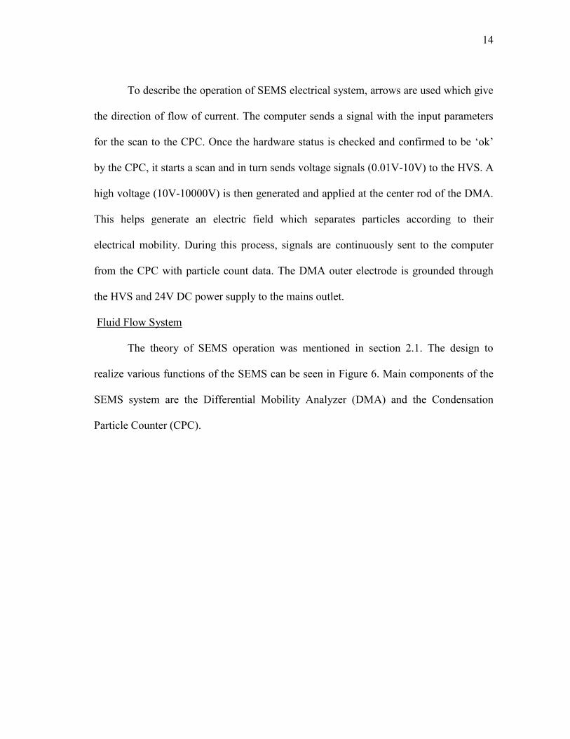
Fluid Flow System
The theory of SEMS operation was mentioned in section 2.1. The design to
realize various functions of the SEMS can be seen in Figure 6. Main components of the
SEMS system are the Differential Mobility Analyzer (DMA) and the Condensation
Particle Counter (CPC).
15
Figure 6: Schematic of the Fluid Flow System for the SEMS system
Differential Mobility Analyzer (DMA): The DMA was purchased from TSI Inc.
(Model #3081) and has the capability to separate particles in the range of 10-1000nm
according to their electrical mobility. It is based on the design of Knutson and Whitby
(1975). The DMA consists of two cylindrical electrodes made of polished stainless steel.
They are insulated from each other at the top by a Teflon spacer and at the bottom by
acetyl-plastic spacer. High voltage is applied to the inner electrode which is 0.369in
(0.937cm) in radius. The outer electrode is 0.772in (1.961cm) radius and distance
between center of aerosol inlet and exit which is the characteristic length is 17.468in
(44.369cm).
16
Condensation Particle Counter (CPC): Condensation Particle Counters (CPC’s)
are devices that grow aerosol particles to optically detectable limits and then count
number of particles per unit volume of gas. They have been in existence since late 19th
century and the first use of CPC was made by John Aitken (1890) to count dust particles
in air. CPC’s have seen a lot of development since then, and the most recent
developments have focused on steady state flow CPC’s. In the design of SEMS, model
3772 CPC from TSI Inc. counted particles in the aerosol. The 3772 had the capability to
measure particles as small as 10nm where as it could count up to 10000 pp/cc.
CPC’s are similar to optical particle counters, however smaller particles can be
counted through the process of growing particles by condensation. The main science
involved in CPC’s is the condensation of vapor onto aerosol particles. The CPC consists
of three sections: saturator, condenser and optical detector. The saturator section is made
of a saturator wick which soaks butanol from a reservoir and saturates the aerosol flow.
The flow then enters the condenser section where vapors get cooled and flow becomes
supersaturated. This leads to condensation on aerosol particles and their growth to sizes
detectable by the optical system. Finally, the concentration of particles is measured in
the optical detector system using a laser diode and photo detector.
Other equipment:
1/4thinch. OD Copper tubing is used to transport aerosol in the Fluid Flow
System. To control flow in the system, two needle valves (Swagelok) and a 6.5 SLM
critical orifice from O’Keefe Controls Co. were used. Compression fittings were used at
all interfaces which prevents outside air from entering the system due to system vacuum.
17
For the filtering of sheath air, a HEPA filter of pore size 0.22micron was applied as seen
in Figure 6. Finally, Thomas Products (Model # 2688VE44) pump provided vacuum to
the SEMS system.
A Polonim-210 strip from AMSTAT Industries Inc. (500 Microcurie) encased in
a stainless steel cylindrical casing provided a known bipolar charge distribution to the
aerosol particles. As Polonium-210 is radioactive, it releases alpha particles which ionize
the air molecules in the casing. As the aerosol particles pass through the casing they
acquire a known charge distribution which can be predicted by Fuchs Equation
mentioned in Section 2.1.1.
Components discussed above were integrated to form the Fluid Flow System
which is shown in Figure 6. Polydisperse aerosol sample enters the DMA through the
polydisperse flow inlet located at top of the DMA. The flow is controlled at 1SLM by a
needle valve and the bipolar charger adds a known charge distribution to the aerosol.
Simultaneously, sheath air is being pulled into the DMA through the sheath air inlet after
undergoing filtration. A high voltage applied at the center rod aids in attracting particles
within a narrow range of mobility which exit through the monodisperse flow outlet at
1L/min. The monodisperse aerosol then flows through the CPC where the particle
concentration is determined. Finally, the remaining aerosol flows out through the excess
air outlet along with sheath air and meets the monodisperse aerosol exhausted from the
CPC. The excess air flow is controlled by a 6.5SLM critical orifice. The flow is finally
exhausted through a pump to the fume hood.
18
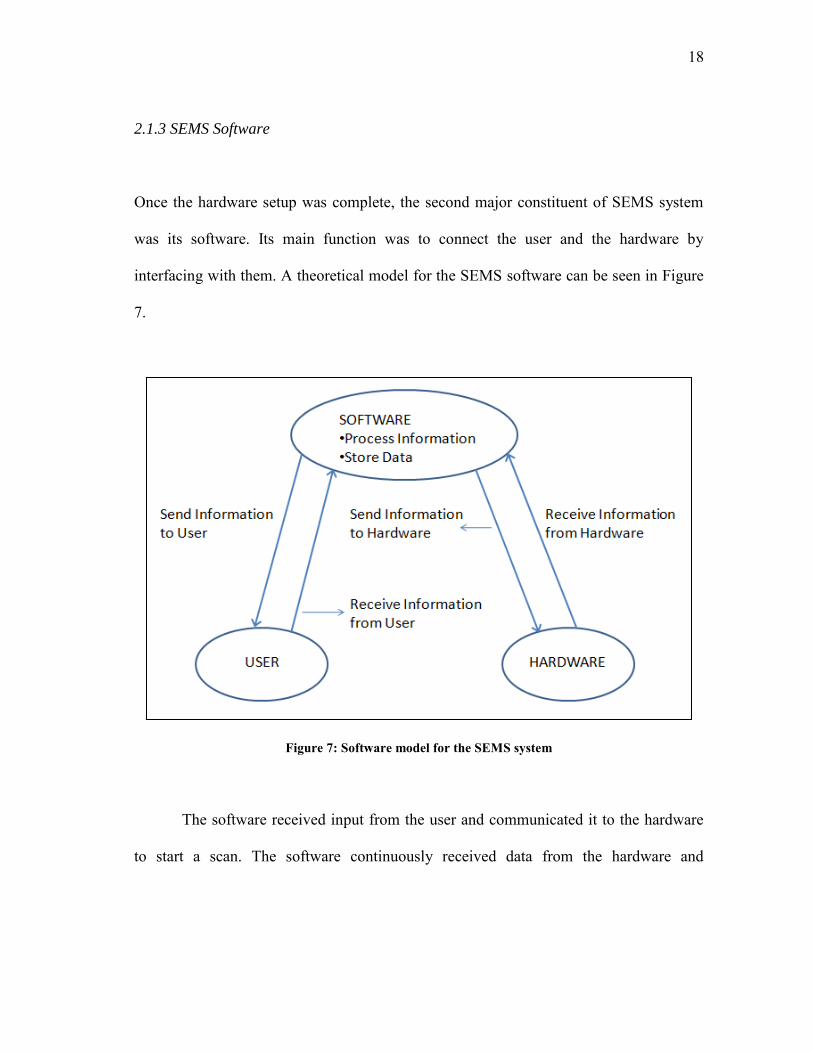
2.1.3 SEMS Software
Once the hardware setup was complete, the second major constituent of SEMS system
was its software. Its main function was to connect the user and the hardware by
interfacing with them. A theoretical model for the SEMS software can be seen in Figure
7.
Figure 7: Software model for the SEMS system
The software received input from the user and communicated it to the hardware
to start a scan. The software continuously received data from the hardware and
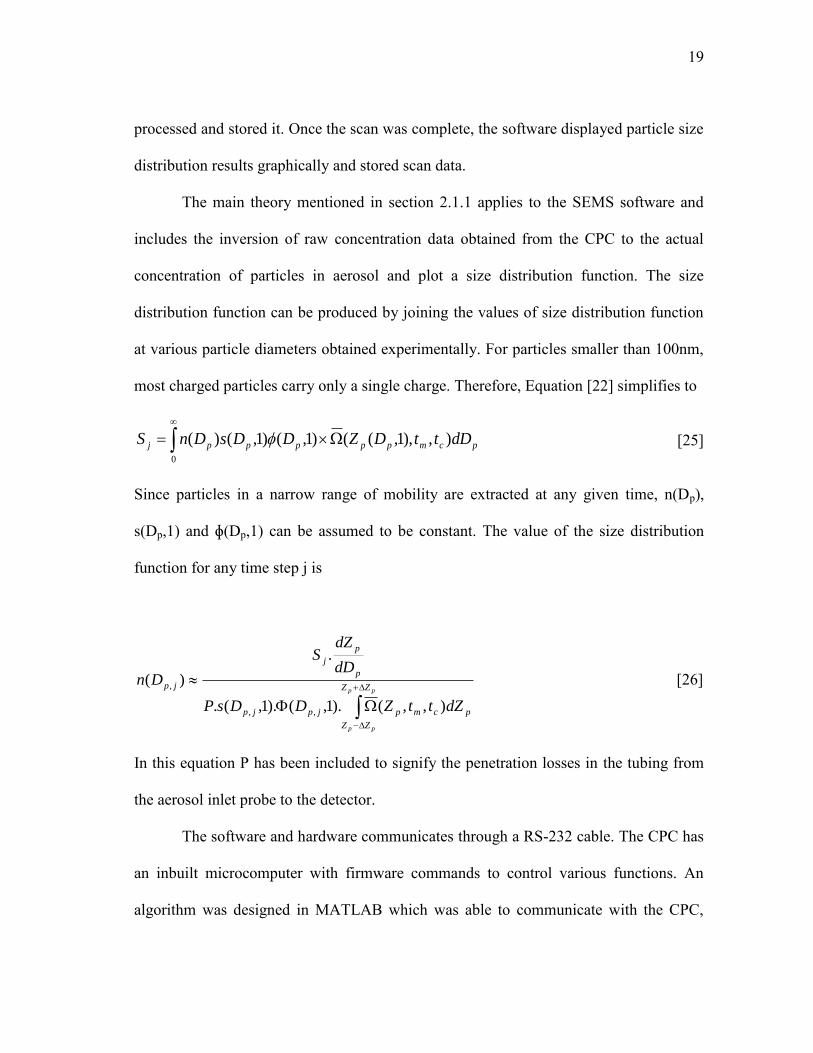
19
processed and stored it. Once the scan was complete, the software displayed particle size
distribution results graphically and stored scan data.
The main theory mentioned in section 2.1.1 applies to the SEMS software and
includes the inversion of raw concentration data obtained from the CPC to the actual
concentration of particles in aerosol and plot a size distribution function. The size
distribution function can be produced by joining the values of size distribution function
at various particle diameters obtained experimentally. For particles smaller than 100nm,
most charged particles carry only a single charge. Therefore, Equation [22] simplifies to
0
),),1,(()1,()1,()( pcmpppppj dDttDZDDsDnS
[25]
Since particles in a narrow range of mobility are extracted at any given time, n(Dp),
s(Dp,1) and ɸ(Dp,1) can be assumed to be constant. The value of the size distribution
function for any time step j is
pp
pp
ZZ
ZZ
pcmpjpjp
p
p
j
jp
dZttZDDsP
dD
dZS
Dn
),,().1,().1,(.
.
)(
,,
,
[26]
In this equation P has been included to signify the penetration losses in the tubing from
the aerosol inlet probe to the detector.
The software and hardware communicates through a RS-232 cable. The CPC has
an inbuilt microcomputer with firmware commands to control various functions. An
algorithm was designed in MATLAB which was able to communicate with the CPC,
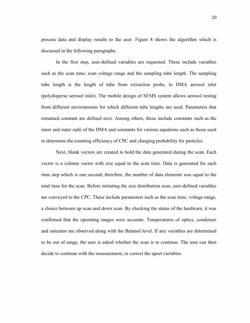
20
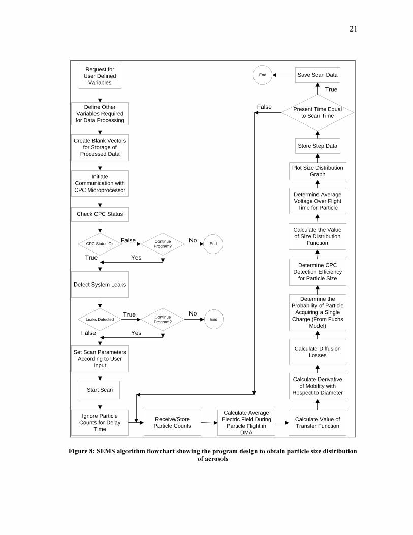
process data and display results to the user. Figure 8 shows the algorithm which is
discussed in the following paragraphs.
In the first step, user-defined variables are requested. These include variables
such as the scan time, scan voltage range and the sampling tube length. The sampling
tube length is the length of tube from extraction probe, to DMA aerosol inlet
(polydisperse aerosol inlet). The mobile design of SEMS system allows aerosol testing
from different environments for which different tube lengths are used. Parameters that
remained constant are defined next. Among others, these include constants such as the
inner and outer radii of the DMA and constants for various equations such as those used
to determine the counting efficiency of CPC and charging probability for particles.
Next, blank vectors are created to hold the data generated during the scan. Each
vector is a column vector with size equal to the scan time. Data is generated for each
time step which is one second; therefore, the number of data elements was equal to the
total time for the scan. Before initiating the size distribution scan, user-defined variables
are conveyed to the CPC. These include parameters such as the scan time, voltage range,
a choice between up scan and down scan. By checking the status of the hardware, it was
confirmed that the operating ranges were accurate. Temperatures of optics, condenser
and saturator are observed along with the Butanol level. If any variables are determined
to be out of range, the user is asked whether the scan is to continue. The user can then
decide to continue with the measurement, or correct the upset variables.
21
Request for
User Defined
Variables
End
Define Other
Variables Required
for Data Processing
Create Blank Vectors
for Storage of
Processed Data
Initiate
Communication with
CPC Microprocessor
Check CPC Status
Detect System Leaks
CPC Status OkContinue
Program?
EndLeaks DetectedContinue
Program?
Set Scan Parameters
According to User
Input
Start Scan
Ignore Particle
Counts for Delay
Time
Receive/Store
Particle Counts
Calculate Average
Electric Field During
Particle Flight in
DMA
Calculate Value of
Transfer Function
Calculate Derivative
of Mobility with
Respect to Diameter
Calculate Diffusion
Losses
Determine the
Probability of Particle
Acquiring a Single
Charge (From Fuchs
Model)
Determine CPC
Detection Efficiency
for Particle Size
Calculate the Value
of Size Distribution
Function
Determine Average
Voltage Over Flight
Time for Particle
Plot Size Distribution
Graph
Store Step Data
Present Time Equal
to Scan Time
Save Scan DataEnd
False No
Yes
Yes
True
False
True No
True
False
Figure 8: SEMS algorithm flowchart showing the program design to obtain particle size distribution of aerosols
22
The next step in the algorithm involves detecting leakage status in the hardware.
Sheath air passes through a HEPA filter before entering the system. This leads to particle
free air and when no voltage was applied at the DMA, the particle concentration is
observed to be zero. Due to vacuum in the system, a leak in the plumbing would cause
particles other than the aerosol particles to enter the system. The concentration is
increased due to this and often results in overshooting the detectable range of CPC.
Concentration is averaged over a period of five seconds. If the concentration is below
0.1pp/cc, the program moves to the next step. Otherwise, the user is provided the option
of discontinuing the program and checking the hardware for leaks. Once the scan is
initiated, a time delay exists between particles exiting the DMA monodisperse outlet and
reaching the CPC particle detector. These particles travel through the interfacing
plumbing and internal CPC tubing. The delay time was found to be 0.507 seconds. All
particles detected by the CPC counter are thus ignored during this interval.
In the next step of the algorithm, the computer receives and stores particle count
data in the blank vectors created earlier. The CPC counts particles every 0.1 seconds and
sends these values to the program buffer. The program receives these values and
averages counts over 1 second, to find the particle concentration. The particle
concentration data is then combined with other parameters for each time step to
determine the size distribution function, as discussed in the following paragraphs.
Worthy of mention in this process was gaining an understanding of the process of
receiving the particle counts from the CPC microprocessor. A first attempt at receiving
information from the CPC was made by considering that firmware commands are
23
required to acquire particle counts. Erratic data received after implementing a number of
firmware commands resulted in temporary discontinuation of real-time size distribution
analysis. A Microsoft Excel spreadsheet was developed with data inversion algorithm.
Particle counts obtained through separate software are integrated within the algorithm
for obtaining offline size distribution measurements. Due to lack of automation, this
process proved to be time consuming and it was decided to gain deeper understanding of
the process of receiving counts from the CPC microprocessor. After a number of trials,
the process of receiving particle counts was realized. Particle counts are sent by the CPC
microprocessor to the software buffer, which is a temporary storage for external data.
The temporary data is collected by the SEMS software as it becomes available and
stored in a blank vector as discussed earlier. Once particle counts are received by the
software, the rest of the parameters required for data inversion are processed internally.
The average electric field is found using Equation [12]
211
1ln
)()(
rrr
tVtE
[27]
Finding the average electric field involves determining the voltage ramp function
executed by the CPC. This is done by recording the ramping voltage at the CPC analog
outlet using a multimeter and curve fitting the data to obtain an equation for the voltage
ramping function. Equation [28] shows this relation.
tSVtV exp)(
[28]
Here, V(t) is the voltage at time t, SV is the start voltage and τ is the time constant and is
defined in Equation [29].
24
IV
EV
ST
ln
[29]
where ST is the scan time, and EV is the end voltage. Only a fraction of particles
entering the DMA through the aerosol inlet, exit the DMA as monodisperse flow. For
every time step, this fraction was expressed by determining the transfer function as for a
range of mobility as shown in Equation [26]. Again the values of the transfer function
and average electric field were stored in the column vectors.
Diffusion losses take place in the plumbing while particles travel from the DMA
outlet to the particle detector. Particles lost to the walls of the tubes through diffusion
can be accounted for by finding the fraction of particles that exit the tubes (Hinds 1999).
This is given by:
77.350.51 32 P for ξ < 0.009
1.70exp0975.05.11exp819.0 P for ξ ≥ 0.009 [30]
where ξ is the dimensionless deposition parameter and can be defined as:
Q
DL [31]
where D is the diffusion coefficient, L is the length of tubing and Q is the aerosol flow
rate in tubing.
Finally, particles are charged in a Bipolar charger leading to a particle of
diameter Dp acquiring a charge i of s(Dp,i). Assuming single charge on the particles,
Fuchs’ model can be used to predict the charging probability. Equation predicting the
25
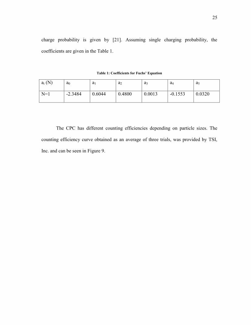
charge probability is given by [21]. Assuming single charging probability, the
coefficients are given in the Table 1.
Table 1: Coefficients for Fuchs’ Equation
ai (N) a0 a1 a2 a3 a4 a5
N=1 -2.3484 0.6044 0.4800 0.0013 -0.1553 0.0320
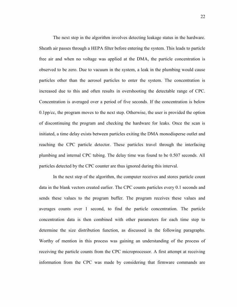
The CPC has different counting efficiencies depending on particle sizes. The
counting efficiency curve obtained as an average of three trials, was provided by TSI,
Inc. and can be seen in Figure 9.
26
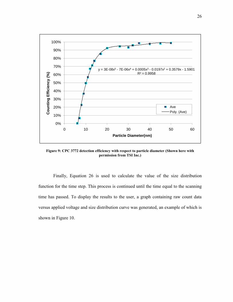
Figure 9: CPC 3772 detection efficiency with respect to particle diameter (Shown here with permission from TSI Inc.)
Finally, Equation 26 is used to calculate the value of the size distribution
function for the time step. This process is continued until the time equal to the scanning
time has passed. To display the results to the user, a graph containing raw count data
versus applied voltage and size distribution curve was generated, an example of which is
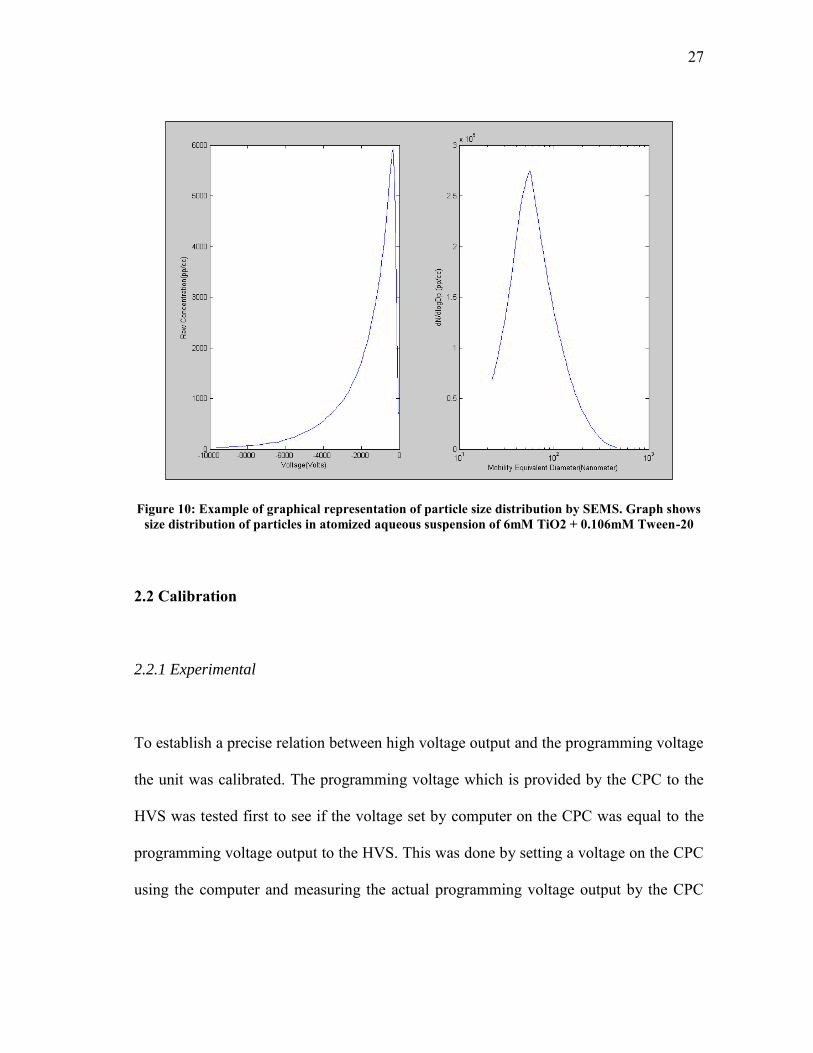
shown in Figure 10.
y = 3E-08x5 - 7E-06x4 + 0.0005x3 - 0.0197x2 + 0.3579x - 1.5901R² = 0.9958
0%
10%
20%
30%
40%
50%
60%
70%
80%
90%
100%
0 10 20 30 40 50 60
Co
un
tin
g E
ffic
ien
cy (
%)
Particle Diameter(nm)
Ave
Poly. (Ave)
27
Figure 10: Example of graphical representation of particle size distribution by SEMS. Graph shows size distribution of particles in atomized aqueous suspension of 6mM TiO2 + 0.106mM Tween-20
2.2 Calibration
2.2.1 Experimental
To establish a precise relation between high voltage output and the programming voltage
the unit was calibrated. The programming voltage which is provided by the CPC to the
HVS was tested first to see if the voltage set by computer on the CPC was equal to the
programming voltage output to the HVS. This was done by setting a voltage on the CPC
using the computer and measuring the actual programming voltage output by the CPC

28
analog output port. Once it was confirmed that the CPC set and output voltage values
were equal, the relation between CPC output voltage (0.01V-10V) and the HVS output
(10-10000V) was determined. Although information provided by the HVS manufacturer
indicates that the relation is HV=1000PV where PV and HV are the programming
voltage input and high voltage output respectively, this was not the case. A multimeter
measured high voltage output from HVS while the CPC provided the programming
voltage to it. The programming voltage on the CPC was set through the computer using
firmware commands for the CPC microcomputer. As the highest voltage measured by
the multimeter was 600V, the relation between PV and TV up to 600V of high voltage
output was assumed to hold true for the entire range.
Testing the high voltage supply was required to confirm the actual range of
voltages that it was functional in, as opposed to the given specifications. Along with this,
an appropriate scan time needed to be determined in which a significant lag would not be
observed between theoretical ramping function and the actual high voltage. The
minimum functioning voltage was found by experimentally determining the settling time
for an increment of 10V from the minimum voltage. This was the time between setting a
voltage at the CPC and getting a stable output from the HVS. The criterion for selection
of minimum voltage was that the settling time would be less than 5 sec. The minimum
functioning voltage was 42V and it took approximately 3s to reach a stable value of 52V
at the HVS output.
29
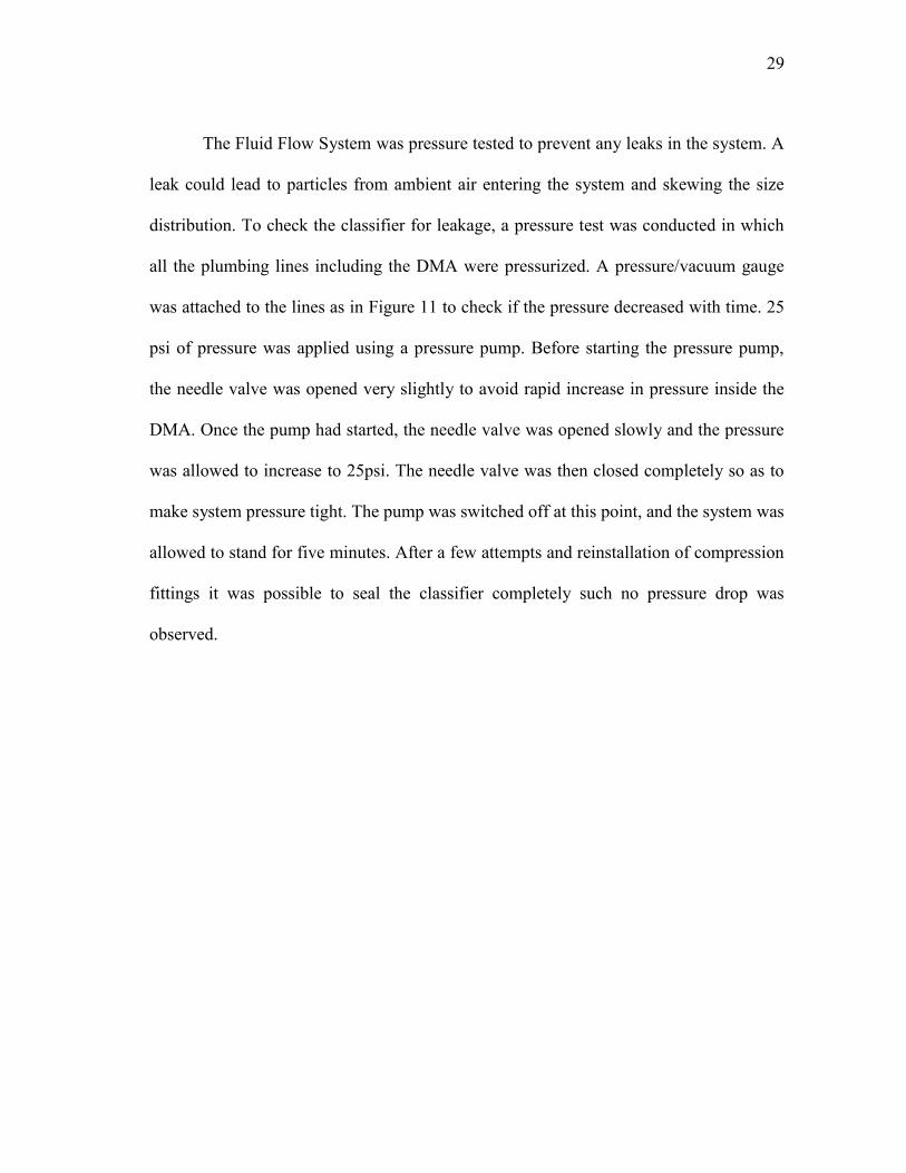
The Fluid Flow System was pressure tested to prevent any leaks in the system. A
leak could lead to particles from ambient air entering the system and skewing the size
distribution. To check the classifier for leakage, a pressure test was conducted in which
all the plumbing lines including the DMA were pressurized. A pressure/vacuum gauge
was attached to the lines as in Figure 11 to check if the pressure decreased with time. 25
psi of pressure was applied using a pressure pump. Before starting the pressure pump,
the needle valve was opened very slightly to avoid rapid increase in pressure inside the
DMA. Once the pump had started, the needle valve was opened slowly and the pressure
was allowed to increase to 25psi. The needle valve was then closed completely so as to
make system pressure tight. The pump was switched off at this point, and the system was
allowed to stand for five minutes. After a few attempts and reinstallation of compression
fittings it was possible to seal the classifier completely such no pressure drop was
observed.
30
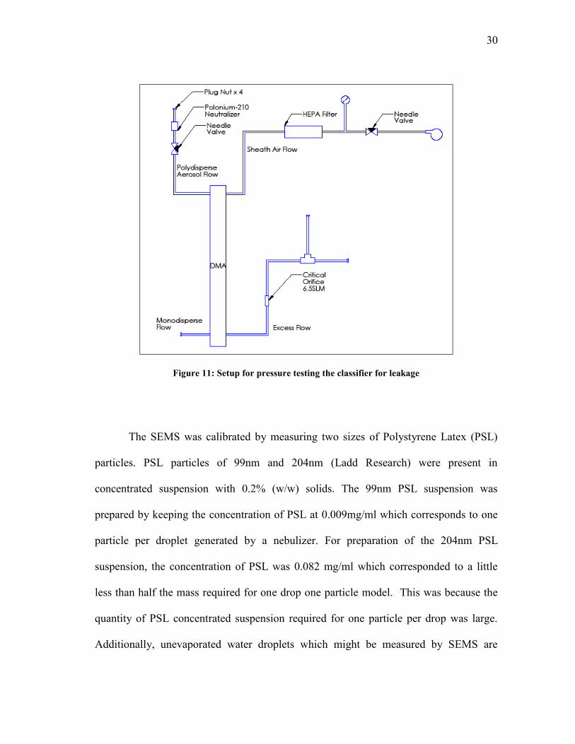
Figure 11: Setup for pressure testing the classifier for leakage
The SEMS was calibrated by measuring two sizes of Polystyrene Latex (PSL)
particles. PSL particles of 99nm and 204nm (Ladd Research) were present in
concentrated suspension with 0.2% (w/w) solids. The 99nm PSL suspension was
prepared by keeping the concentration of PSL at 0.009mg/ml which corresponds to one
particle per droplet generated by a nebulizer. For preparation of the 204nm PSL
suspension, the concentration of PSL was 0.082 mg/ml which corresponded to a little
less than half the mass required for one drop one particle model. This was because the
quantity of PSL concentrated suspension required for one particle per drop was large.
Additionally, unevaporated water droplets which might be measured by SEMS are
31
within the range of 10-80nm and would not interfere with size distribution of 204nm
PSL particles.
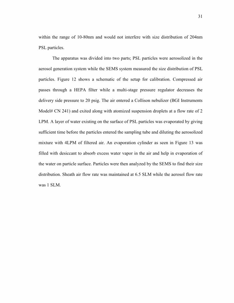
The apparatus was divided into two parts; PSL particles were aerosolized in the
aerosol generation system while the SEMS system measured the size distribution of PSL
particles. Figure 12 shows a schematic of the setup for calibration. Compressed air
passes through a HEPA filter while a multi-stage pressure regulator decreases the
delivery side pressure to 20 psig. The air entered a Collison nebulizer (BGI Instruments
Model# CN 241) and exited along with atomized suspension droplets at a flow rate of 2
LPM. A layer of water existing on the surface of PSL particles was evaporated by giving
sufficient time before the particles entered the sampling tube and diluting the aerosolized
mixture with 4LPM of filtered air. An evaporation cylinder as seen in Figure 13 was
filled with desiccant to absorb excess water vapor in the air and help in evaporation of
the water on particle surface. Particles were then analyzed by the SEMS to find their size
distribution. Sheath air flow rate was maintained at 6.5 SLM while the aerosol flow rate
was 1 SLM.
32
Figure 12: Apparatus setup for SEMS Calibration
The size distribution measurements of PSL suspension were taken four times for
each suspension. The average mode was then computed from these trials which
represented the diameter of particles at which largest particle number concentration
existed. To determine the mode diameter in actual concentrated suspension, TEM
analysis was conducted. For this, concentrated suspension was kept on a TEM grid and
dried. TEM images were taken for both PSL particle sizes. Particle diameters were
manually measured for individual particles, and the size distribution was found. The
mode diameter from TEM analysis was then compared to the mode diameter obtained
from SEMS measurement.
33
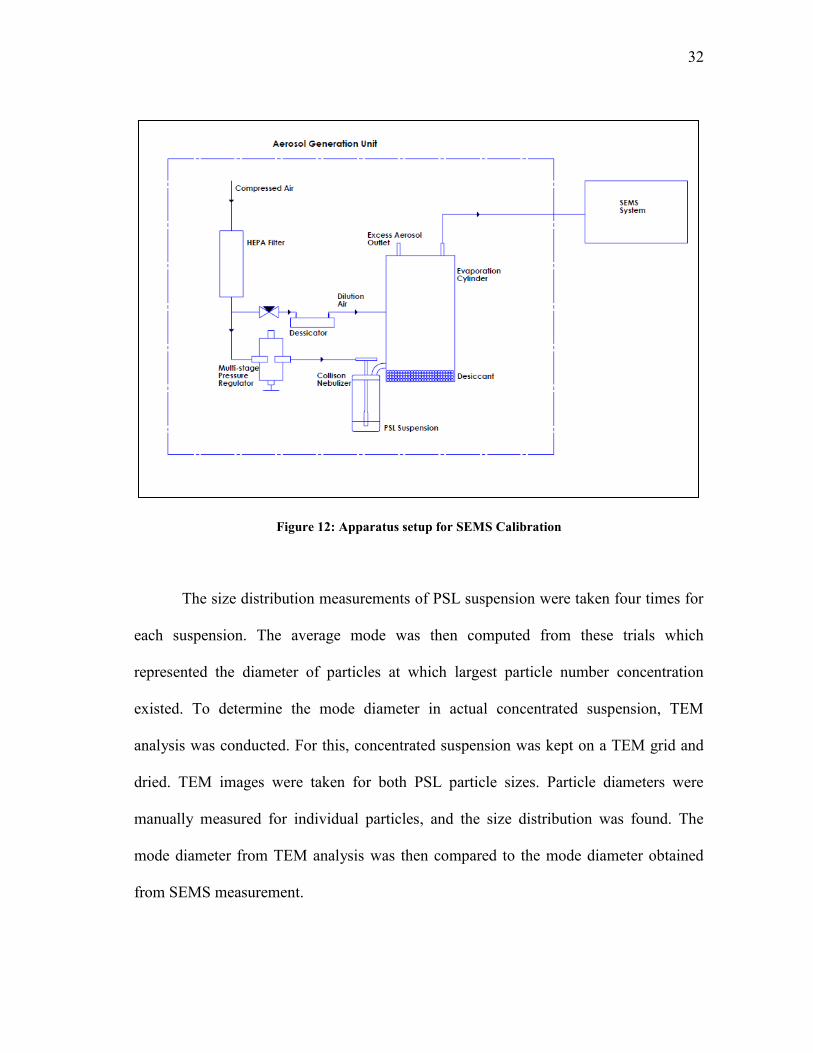
2.2.2 Results and Conclusions
Equation [32] shows the relation between HV and PV.
49.2767.992 PVHV [32]
As high voltage supplies respond slowly near the higher and lower limits of
voltage, a maximum voltage of 9000V was assumed as the upper limit of the HVS. By
reading the responses of HVS with various scan times, 95sec was the minimum time
which prevented significant lag between theoretical and high voltages. A graph
comparing the theoretical and high voltage responses is shown in Figure 13. Here the
theoretical response is the CPC ramping function which was applied in the program to
invert data. The average difference between theoretical and high voltage was
approximately 6% with higher difference close to the starting voltage in the scan. It can
be concluded from this calibration experiment that the high voltage output from HVS
follows the theoretical voltage closely.
34
Figure 13: Comparison of theoretical or programming voltage provided to HVS and its high voltage response
Figure 14: TEM image of 99nm PSL particles
0
1000
2000
3000
4000
5000
6000
7000
8000
9000
10000
0 20 40 60 80 100
Vo
ltag
e (
Vo
lts)
Scan Time (Sec)
Theoretical Voltage
High Voltage Output
35
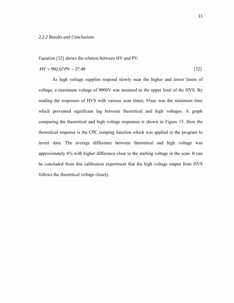
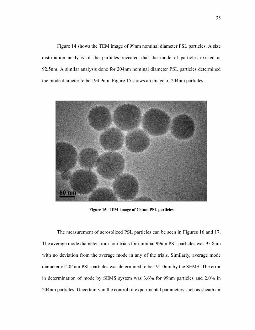
Figure 14 shows the TEM image of 99nm nominal diameter PSL particles. A size
distribution analysis of the particles revealed that the mode of particles existed at
92.5nm. A similar analysis done for 204nm nominal diameter PSL particles determined
the mode diameter to be 194.9nm. Figure 15 shows an image of 204nm particles.
Figure 15: TEM image of 204nm PSL particles
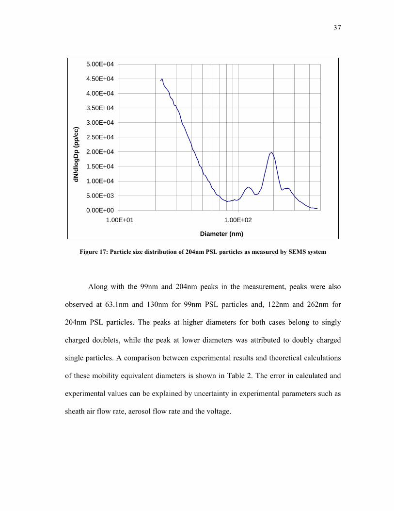
The measurement of aerosolized PSL particles can be seen in Figures 16 and 17.
The average mode diameter from four trials for nominal 99nm PSL particles was 95.8nm
with no deviation from the average mode in any of the trials. Similarly, average mode
diameter of 204nm PSL particles was determined to be 191.0nm by the SEMS. The error
in determination of mode by SEMS system was 3.6% for 99nm particles and 2.0% in
204nm particles. Uncertainty in the control of experimental parameters such as sheath air
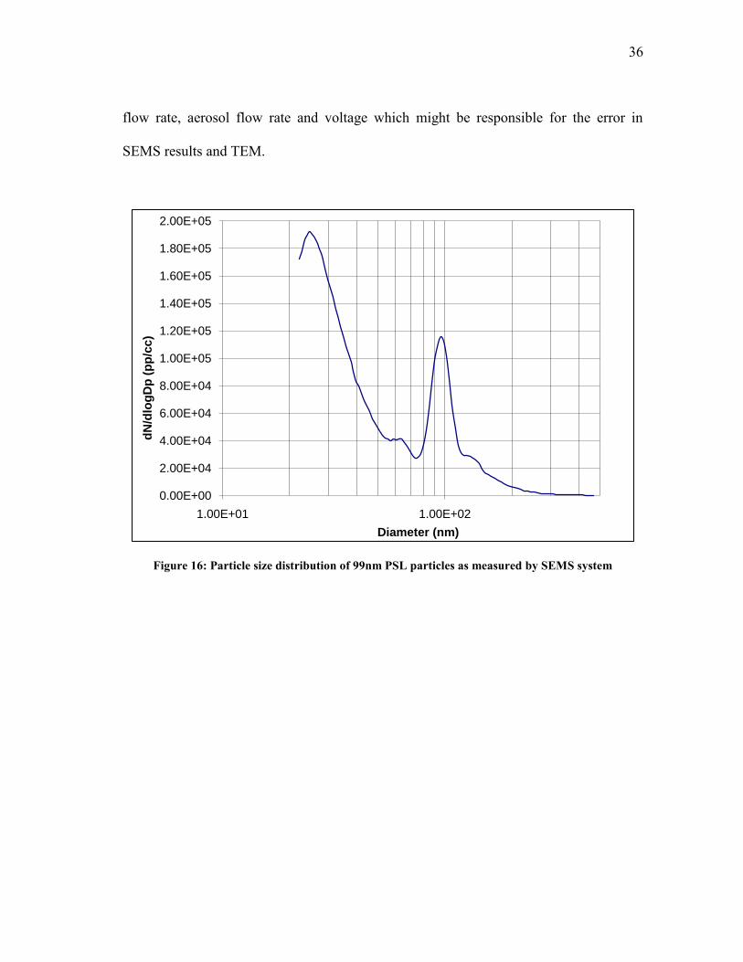
36
flow rate, aerosol flow rate and voltage which might be responsible for the error in
SEMS results and TEM.
Figure 16: Particle size distribution of 99nm PSL particles as measured by SEMS system
0.00E+00
2.00E+04
4.00E+04
6.00E+04
8.00E+04
1.00E+05
1.20E+05
1.40E+05
1.60E+05
1.80E+05
2.00E+05
1.00E+01 1.00E+02
dN
/dlo
gD
p (
pp
/cc)
Diameter (nm)
37
Figure 17: Particle size distribution of 204nm PSL particles as measured by SEMS system
Along with the 99nm and 204nm peaks in the measurement, peaks were also
observed at 63.1nm and 130nm for 99nm PSL particles and, 122nm and 262nm for
204nm PSL particles. The peaks at higher diameters for both cases belong to singly
charged doublets, while the peak at lower diameters was attributed to doubly charged
single particles. A comparison between experimental results and theoretical calculations
of these mobility equivalent diameters is shown in Table 2. The error in calculated and
experimental values can be explained by uncertainty in experimental parameters such as
sheath air flow rate, aerosol flow rate and the voltage.
0.00E+00
5.00E+03
1.00E+04
1.50E+04
2.00E+04
2.50E+04
3.00E+04
3.50E+04
4.00E+04
4.50E+04
5.00E+04
1.00E+01 1.00E+02
dN
/dlo
gD
p (
pp
/cc)
Diameter (nm)
38
Table 2: An explanation for additional peaks observed in size distribution of 99nm and 204nm PSL particles
Particle Description
Experimental
Mobility
Equivalent
Diameter (nm)
Calculated
Mobility
Equivalent
Diameter (nm)
Percentage
Difference
(%)
99nm
Singly charged Doublet 63.1 67.2 6.1
Doubly charge single
particle 130 132 1.5
204nm
Singly charged doublet 262 269 2.6
Doubly charge single
particle 122 132 7.6
It is observed in Figures 16 and 17 that certain particles are observed before the
PSL particles. These particles are due to aerosolized de-ionized water and surfactants
present in the PSL suspension (Zhang et al. 1995). Particles in De-ionized water will be
discussed in greater detail in a later section.
39
3. A STUDY OF GENERATION OF TITANIUM DIOXIDE PARTICLES USING
A COLLISON NEBULIZER
3.1 Introduction
Development and research in nanotechnology has accelerated since its first application
of IBM logo depiction (Hood 2004). Nanoparticles exhibit a number of unique physical
and chemical properties due to their large specific surface areas (Shimada et al. 2009).
Due to their properties nanoparticles have found application in a number of different
fields such as medicine, agriculture, industry, environment and engineering (Navrotsky
2000). For example, magnetite is used to make ferrofluids, which can be used as
nanoelectromechanical (NEMS) systems, such as nanomotors, nanopumps,
nanogenerators and nanoactuators (Zahn 2001). Selective manipulation and probing of
biological systems can be accomplished by nanoengineered magnetic particles (Reich et
al. 2003).
As with all new technologies, along with potential benefits there are a number of
risks involved in nanotechnology. The risks can be to the environment and humans. For
example, there is risk of exposure to the entire ecosystem through water and soil.
Furthermore, the concentration of engineered nanoparticles increases in direct proportion
to their use in society. Toxicology studies of micron-sized particles have been done
extensively in medical studies. The coal miner’s disease and asbestosis are two examples
of diseases caused due to inhalation exposure to micron-sized particles. It has been
40
found that the nanoparticles are more toxic than micron-sized particles in similar doses
due to their smaller size (Colvin 2003).
Due to risks of nanotechnology and exposure to nanoparticles, there has been
increased concern about the health effect of nanoparticles. Manufactured nanoparticles
exist mostly in suspension or dry powder form (Shimada et al. 2009). For inhalation
exposure studies of nanoparticles, a constant supply of nanoparticles with size
distribution similar to original powder or suspension is required.
In this study, the Collison nebulizer was studied as a source of nanoparticle
generation from suspensions. The size distribution and concentration stability of
Titanium dioxide particles generated by the nebulizer were studied and compared against
single particle size distribution present in powder form. Surfactants are known to modify
the interaction potential of particles in a suspension and hence give stability and
increasing repulsive force between particles(Schick 1967). In this study, the effect of
surfactant on particle size distribution of TiO2 was also analyzed.
3.2 Theory/Model
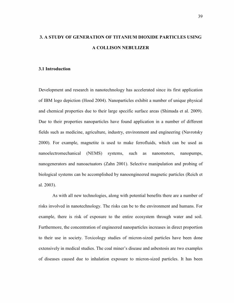
The model to study aerosol generated by a Collison nebulizer is shown in Figure 18.
Liquid droplets containing powder particles can be generated by a nebulizer and allowed
to dry in a drying tank. The size distribution of dry particles could then be measured
using a SEMS system. The Collison nebulizer breaks a stream of liquid into minute
droplets. These droplets are impacted against a glass jar and only the smaller ones escape
41
to the exit nozzle. The concentration of powder in the suspension can be such that each
droplet contains only one particle. This was done so that the aerosol generated had
similar size distribution as the single particles in powder.
Figure 18: Model for study of aerosol generated by Collison nebulizer
From a known size distribution of droplets generated by the Collison nebulizer, it
is possible to calculate the average size of droplet generated by the nebulizer. A drying
cylinder which provides sufficient residence time to dry the particles can be used to
produce completely dried particles whose size distribution is measurable by the SEMS
system. To study the aerosol generated by the nebulizer this model was applied and is
explained in detail in the following sections.
3.3 Experimental
The experimental setup for measurement of the size distribution of Titanium dioxide
particles is shown in Figure 19. A Collison nebulizer (BGI Incorporated Model# CN
241) nebulized TiO2 particles from suspension in the glass jar. Compressed air was
provided to the nebulizer at 20psi after filtering it through a high efficiency particulate
air (HEPA) filter. The pressure was regulated by a multi-stage regulator which delivered
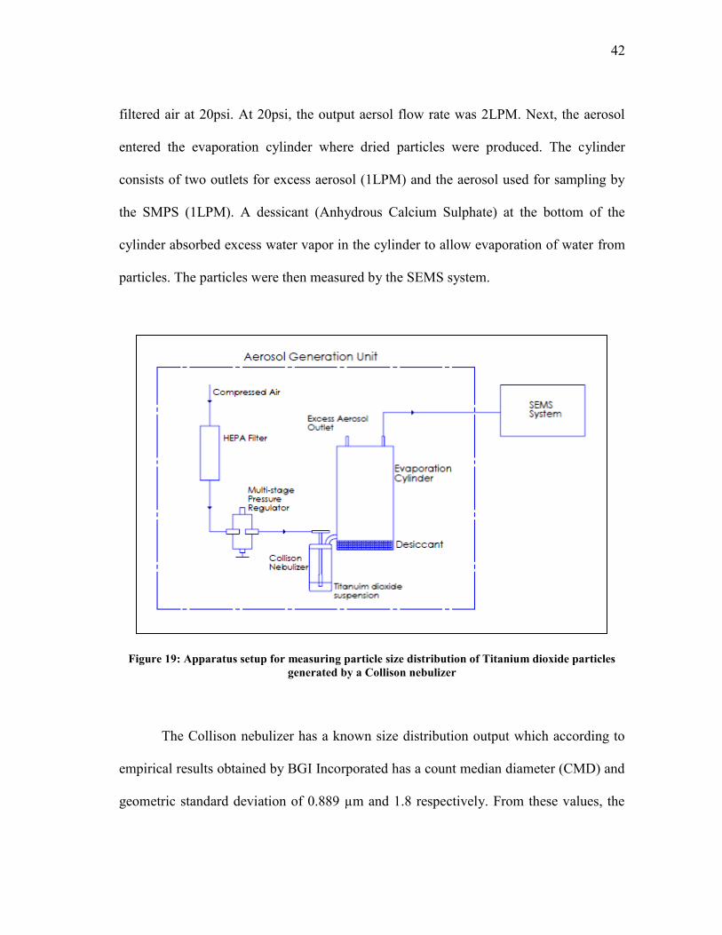
42
filtered air at 20psi. At 20psi, the output aersol flow rate was 2LPM. Next, the aerosol
entered the evaporation cylinder where dried particles were produced. The cylinder
consists of two outlets for excess aerosol (1LPM) and the aerosol used for sampling by
the SMPS (1LPM). A dessicant (Anhydrous Calcium Sulphate) at the bottom of the
cylinder absorbed excess water vapor in the cylinder to allow evaporation of water from
particles. The particles were then measured by the SEMS system.
Figure 19: Apparatus setup for measuring particle size distribution of Titanium dioxide particles generated by a Collison nebulizer
The Collison nebulizer has a known size distribution output which according to
empirical results obtained by BGI Incorporated has a count median diameter (CMD) and
geometric standard deviation of 0.889 µm and 1.8 respectively. From these values, the
43
average size droplet was found to have a diameter of 4.49 µm. For this droplet, it would
take approximately 3 seconds to dry completely at a relative humidity (RH) of 96.7%
which was found experimentally using a humidity meter. The value of RH was noted
after a stable condition was reached and the RH did not change more than 0.2% for more
than 5 minutes. A residence time of 93.9 seconds inside the drying cylinder ensured
sufficient time for even the larger particles to dry completely before being sampled by
the SEMS.
The solution was made such that each droplet contained one particle of TiO2 the
calculation for which can be seen in the Appendix. It was found that 0.08mg/ml or
1.06mM of TiO2 was required for each drop to contain one particle. A range of
concentrations of TiO2 were chosen to study the aerosolization of TiO2 suspension.
These ranged from 0.5mM to 9mM. Size distribution measurements of 5 concentrations
of TiO2 suspensions were made which included 0.5mM, 1mM, 3mM, 6mM and 9mM.
Five size distribution measurements for each concentration were taken to observe trends
in the size distribution with time. To compare size distribution of aerosolized particles
with single particles present in powder, TEM was conducted as well. Particles below
30nm were not included in the size distribution analysis due to their large quantity and
undefined boundaries. Most of the particles were either under larger particles or in
clusters such that their boundaries were not clearly discernible in the TEM image.
To observe the aggregation of TiO2 particles in the solution, Dynamic Light
Scattering (DLS) measurements were conducted with a 1mM suspension. DLS
measurements are useful in determining the size distribution of particles in a suspension.
44
The suspension to be sampled for DLS was probe sonicated for 5 minutes and separated
into two parts. While the size distribution of the first sample was taken immediately, the
other sample was nebulized using a Collison nebulizer for 30 minutes. The results of
these studies can be seen in the next section.
To check the effect of surfactant on size distribution of aerosolized TiO2, Tween-
20 (Polyoxyethylene (2) Sorbitan Monolaurate) was added in different concentrations to
a 6mM TiO2 suspension. A stock solution with 2.0mM Tween-20 was prepared to
facilitate dispensing of the surfactant as it was very viscous in its original form. Critical
Micelle Concentration for a surfactant is the concentration above which micelles are
spontaneously formed. Four different concentration of Tween 20, close to the Critical
Micelle Concentration, 0.042mM (Patist et al. 2000), were added to 6mM TiO2.
3.4 Results and Conclusions
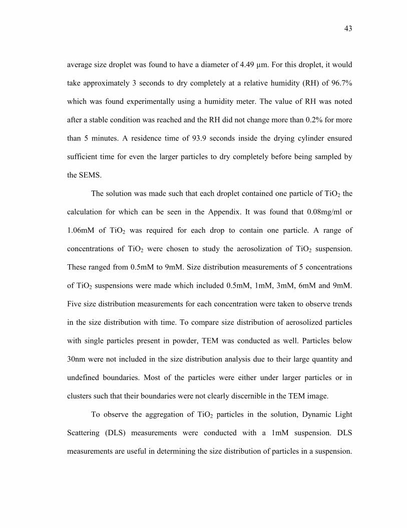
Figure 20 shows a graph of the size distributions for 5 different concentrations of TiO2
suspensions. The peaks that can be seen in the lower end of the size spectrum correspond
to particles between the range of approximately 10nm to 80nm. These are the residual
particles from impurities in water and unevaporated water droplets and possibly TiO2
nanoparticles. Peaks corresponding to the larger diameters (approximately 200nm)
represent the TiO2 particles. This was deduced by running the nebulizer only with DI
water and measuring its size distribution. The size distribution observed had a mode
diameter of approximately 30nm. No secondary peak was observed for DI water. Along
45
with this, the concentration of larger particles increases as the TiO2 in suspension
increases, indicating a correspondence between TiO2 particles and the peak
corresponding to the larger particles.
The unformed peaks for 0.5mM and 1mM indicate low concentration of TiO2
particles. The graph is further skewed by the presence of residual particles. It can also be
observed that concentration of residual particles increases as the number of TiO2
particles in suspension decrease. This can be explained by the larger number of empty
droplets for lower concentrations. Lower TiO2 particles result in more empty droplets
which upon evaporation lead to residual particles. The contribution of unevaporated DI
water droplets to residual droplets had been confirmed and will be discussed in the next
section.
The mode diameters of 3mM, 6mM, and 9mM were found to be 197.5nm,
200.0nm and 195.2nm respectively. The mode diameter corresponds to the average of 5
trials with the same suspension concentration. Thus, there is not much change in the size
mode diameter in this concentration range studied.
46
Figure 20: Particle size distribution of various concentrations of Titanium dioxide suspensions
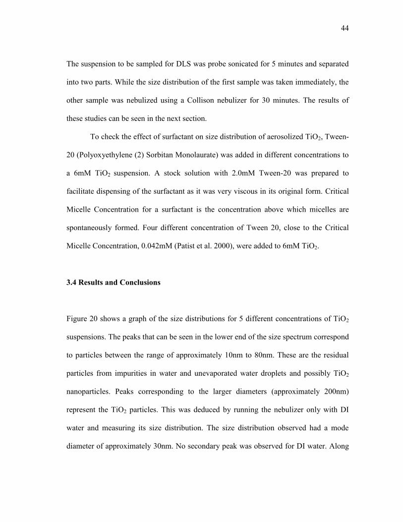
Figure 21: Size distribution of 9.0mM Titanium dioxide suspension for 6 trials taken at different times during Collison nebulizer run
0.00E+00
5.00E+04
1.00E+05
1.50E+05
2.00E+05
2.50E+05
10 100 1,000
dN
/dlo
gD
p (
pp
/cc)
Diameter (nm)
0.5mM
1.0mM
3.0mM
6.0mM
9.0mM
0.00E+00
2.00E+04
4.00E+04
6.00E+04
8.00E+04
1.00E+05
1.20E+05
1.40E+05
1.60E+05
1.00E+01 1.00E+02 1.00E+03
dN
/dlo
gD
p (
pp
/cc)
Diameter (nm)
30 mins
35 mins
40 mins
45 mins
50 mins
120 mins
47
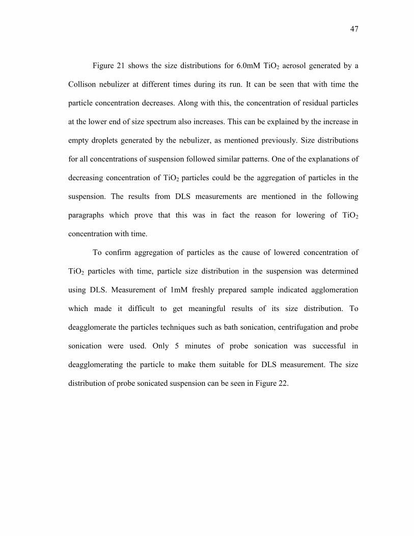
Figure 21 shows the size distributions for 6.0mM TiO2 aerosol generated by a
Collison nebulizer at different times during its run. It can be seen that with time the
particle concentration decreases. Along with this, the concentration of residual particles
at the lower end of size spectrum also increases. This can be explained by the increase in
empty droplets generated by the nebulizer, as mentioned previously. Size distributions
for all concentrations of suspension followed similar patterns. One of the explanations of
decreasing concentration of TiO2 particles could be the aggregation of particles in the
suspension. The results from DLS measurements are mentioned in the following
paragraphs which prove that this was in fact the reason for lowering of TiO2
concentration with time.
To confirm aggregation of particles as the cause of lowered concentration of
TiO2 particles with time, particle size distribution in the suspension was determined
using DLS. Measurement of 1mM freshly prepared sample indicated agglomeration
which made it difficult to get meaningful results of its size distribution. To
deagglomerate the particles techniques such as bath sonication, centrifugation and probe
sonication were used. Only 5 minutes of probe sonication was successful in
deagglomerating the particle to make them suitable for DLS measurement. The size
distribution of probe sonicated suspension can be seen in Figure 22.
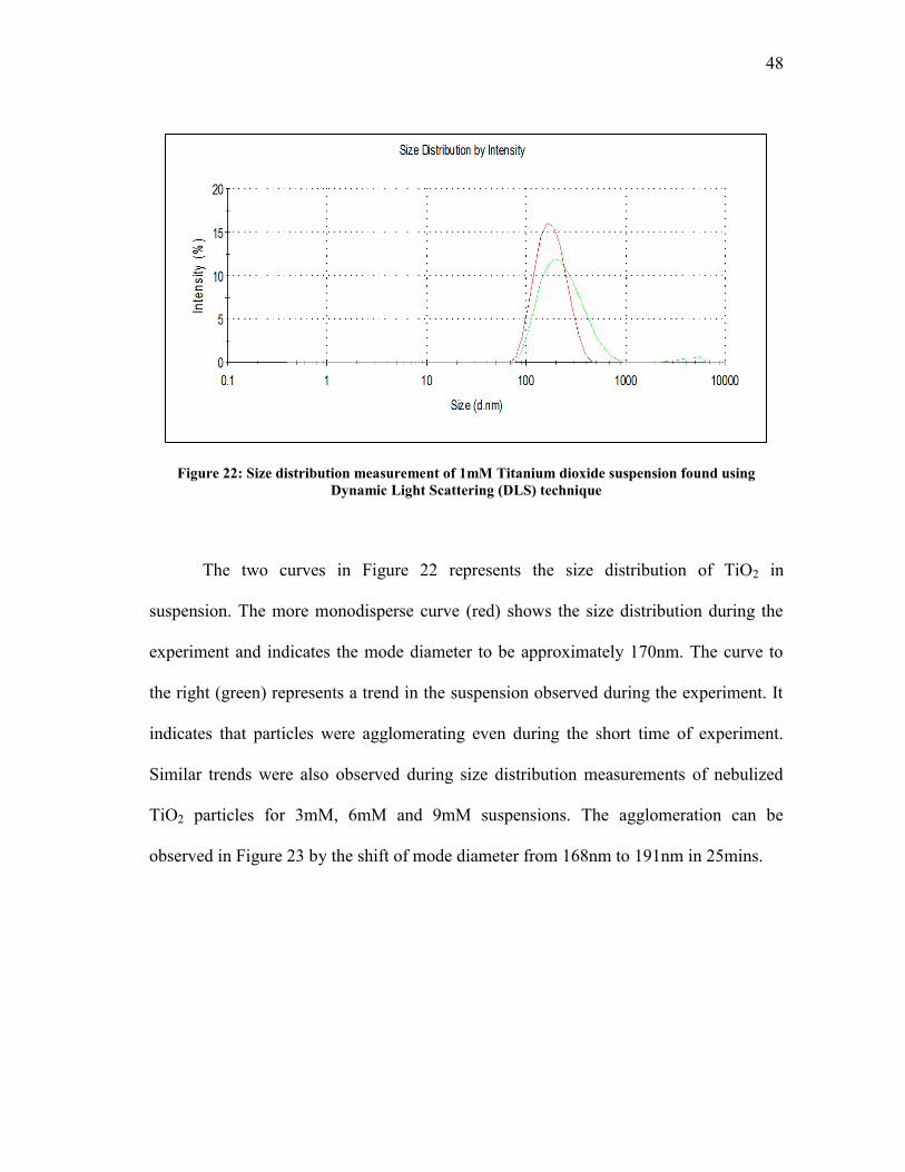
48
Figure 22: Size distribution measurement of 1mM Titanium dioxide suspension found using Dynamic Light Scattering (DLS) technique
The two curves in Figure 22 represents the size distribution of TiO2 in
suspension. The more monodisperse curve (red) shows the size distribution during the
experiment and indicates the mode diameter to be approximately 170nm. The curve to
the right (green) represents a trend in the suspension observed during the experiment. It
indicates that particles were agglomerating even during the short time of experiment.
Similar trends were also observed during size distribution measurements of nebulized
TiO2 particles for 3mM, 6mM and 9mM suspensions. The agglomeration can be
observed in Figure 23 by the shift of mode diameter from 168nm to 191nm in 25mins.
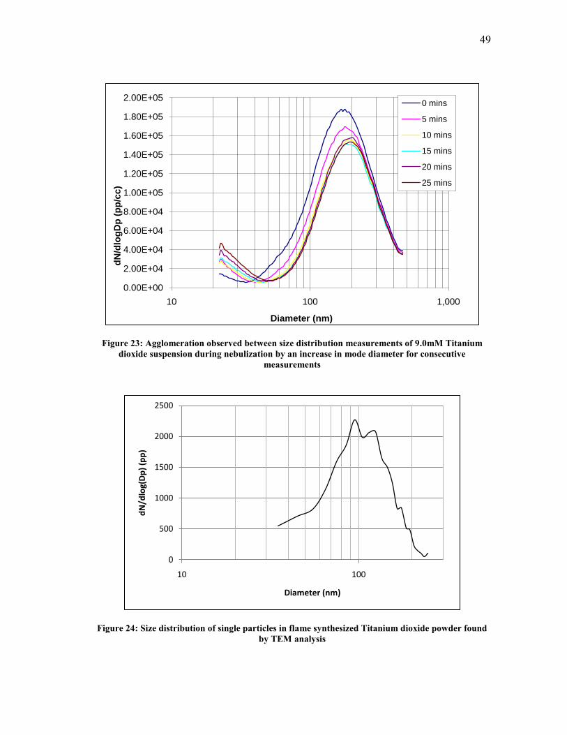
49
Figure 23: Agglomeration observed between size distribution measurements of 9.0mM Titanium dioxide suspension during nebulization by an increase in mode diameter for consecutive
measurements
Figure 24: Size distribution of single particles in flame synthesized Titanium dioxide powder found by TEM analysis
0.00E+00
2.00E+04
4.00E+04
6.00E+04
8.00E+04
1.00E+05
1.20E+05
1.40E+05
1.60E+05
1.80E+05
2.00E+05
10 100 1,000
dN
/dlo
gD
p (
pp
/cc)
Diameter (nm)
0 mins
5 mins
10 mins
15 mins
20 mins
25 mins
0
500
1000
1500
2000
2500
10 100
dN
/dlo
g(D
p)
(pp
)
Diameter (nm)
50
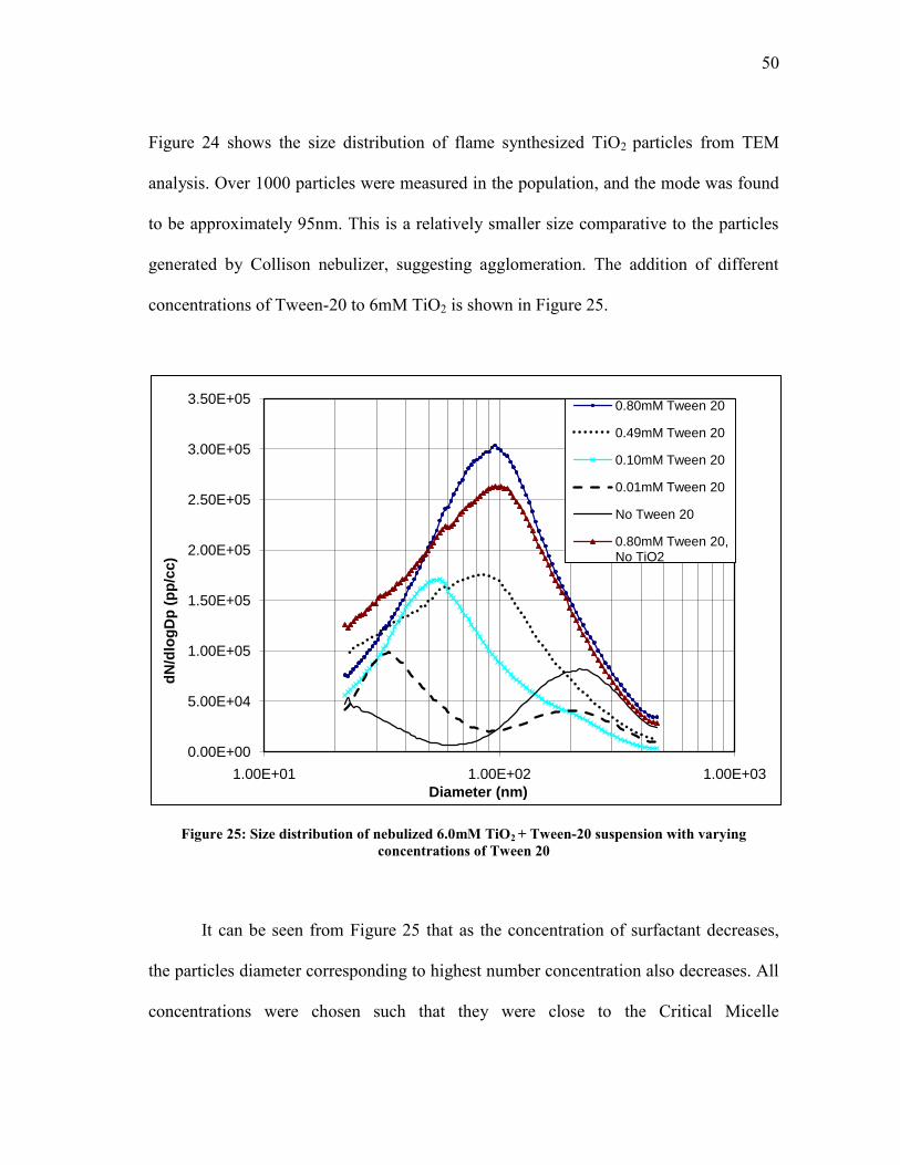
Figure 24 shows the size distribution of flame synthesized TiO2 particles from TEM
analysis. Over 1000 particles were measured in the population, and the mode was found
to be approximately 95nm. This is a relatively smaller size comparative to the particles
generated by Collison nebulizer, suggesting agglomeration. The addition of different
concentrations of Tween-20 to 6mM TiO2 is shown in Figure 25.
Figure 25: Size distribution of nebulized 6.0mM TiO2 + Tween-20 suspension with varying concentrations of Tween 20
It can be seen from Figure 25 that as the concentration of surfactant decreases,
the particles diameter corresponding to highest number concentration also decreases. All
concentrations were chosen such that they were close to the Critical Micelle
0.00E+00
5.00E+04
1.00E+05
1.50E+05
2.00E+05
2.50E+05
3.00E+05
3.50E+05
1.00E+01 1.00E+02 1.00E+03
dN
/dlo
gD
p (
pp
/cc)
Diameter (nm)
0.80mM Tween 20
0.49mM Tween 20
0.10mM Tween 20
0.01mM Tween 20
No Tween 20
0.80mM Tween 20, No TiO2
51
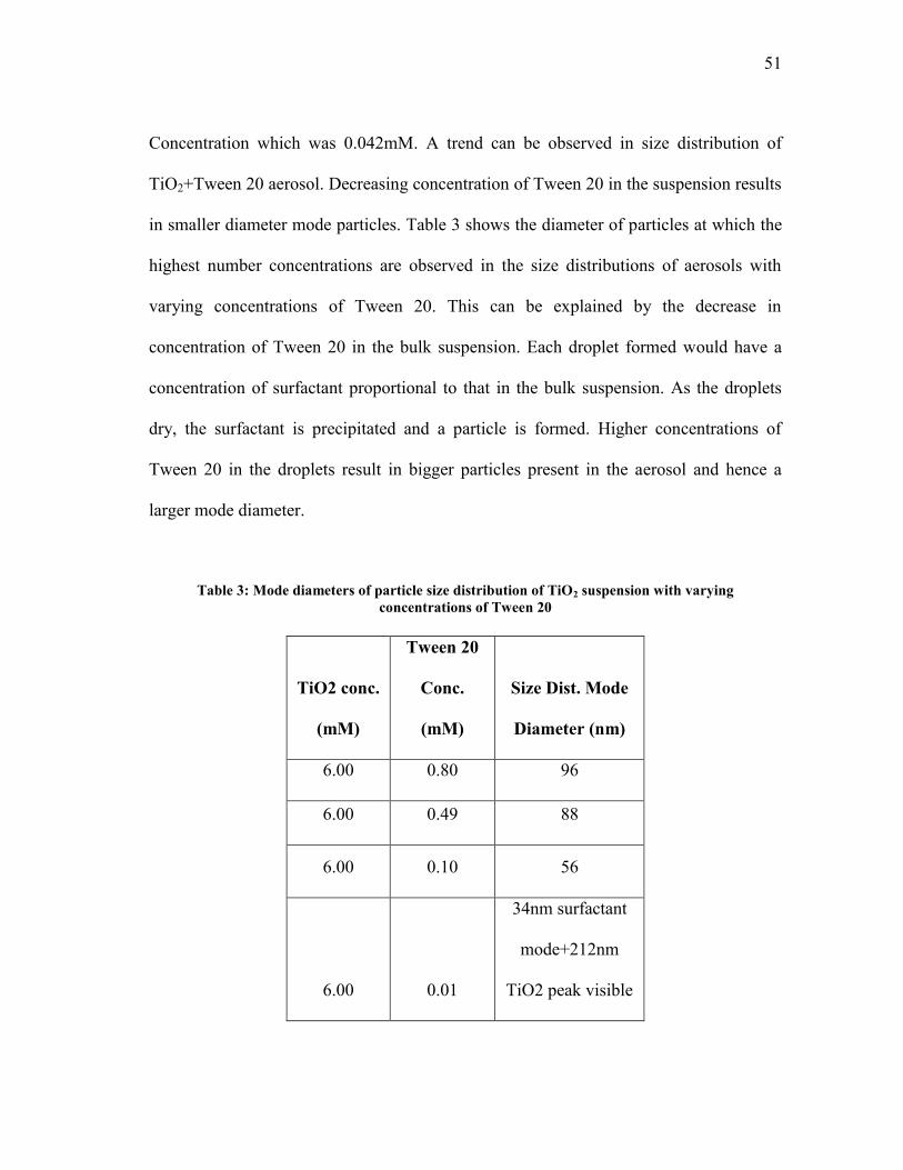
Concentration which was 0.042mM. A trend can be observed in size distribution of
TiO2+Tween 20 aerosol. Decreasing concentration of Tween 20 in the suspension results
in smaller diameter mode particles. Table 3 shows the diameter of particles at which the
highest number concentrations are observed in the size distributions of aerosols with
varying concentrations of Tween 20. This can be explained by the decrease in
concentration of Tween 20 in the bulk suspension. Each droplet formed would have a
concentration of surfactant proportional to that in the bulk suspension. As the droplets
dry, the surfactant is precipitated and a particle is formed. Higher concentrations of
Tween 20 in the droplets result in bigger particles present in the aerosol and hence a
larger mode diameter.
Table 3: Mode diameters of particle size distribution of TiO2 suspension with varying concentrations of Tween 20
TiO2 conc.
(mM)
Tween 20
Conc.
(mM)
Size Dist. Mode
Diameter (nm)
6.00 0.80 96
6.00 0.49 88
6.00 0.10 56
6.00 0.01
34nm surfactant
mode+212nm
TiO2 peak visible
52
It can be observed from Figure 25, that at Tween 20 concentration of 0.01mM,
two peaks are observed. It can be deduced from earlier observations of size distribution
measurement of aerosol with no surfactant that the larger peak with a mode diameter
212nm belongs to the TiO2 particles. This is because 6.0mM TiO2 suspension had a peak
at approximately 200nm. The slight increase in mode diameter with the addition of
surfactant is due to the presence of an additional layer of Tween 20 over the particle
surface. From this observation, it can be concluded that the surfactant does not have
significant effect in emulating single particle distribution observed in powder. A
possible explanation for this is the formation of agglomerates during storage of TiO2
powder. Hard agglomerates, which can be formed due to fusion or interparticle bonds,
cannot be broken by mild forces such as sonication applied during suspension
preparation (Schmoll et al. 2009).
53
4. STUDY OF BACKGROUND PARTICLES IN AEROSOLIZED DE-IONIZED
WATER
4.1 Background
As seen in Section 2.2, for calibrating the SEMS system, a solution of 99nm/204nm
diameter Polystyrene Latex (PSL) particles was made in DI water. It was observed that
certain background particles were present which skewed the size distribution results of
PSL particles. The source of these background particles was determined to be either
compressed air fed into the nebulizer, or the DI water. Analysis of compressed air
determined low concentration of particles with a mode slightly above a 100nm. Thus, DI
water was confirmed to be the source of particles.
Nebulization is a widespread method of converting suspension or solutions to
aerosols. This technique is used in toxicology inhalation studies frequently, especially
for studying the characteristics of nanoparticles. Although DI water is often used as a
solvent in the nebulization process, residual particles are observed which interfere with
the study of particles of concern. Studies have linked the source of these particles to be
dissolved impurities inherent to water, as well as leaching from the container walls.
Furthermore, the chemical composition is not yet known and may be highly variable
(LaFranchi et al. 2003).
Knowledge of particles in DI water can help identify ways for removal of
particles and thus make DI water better suited for applications requiring high level of
54
purity. The main objective of the following work was to determine the chemical
composition of particles observed in DI water.
4.2 Hypothesis/Model
It was hypothesized that the residual particles observed in the calibration process were a
combination of dissolved impurities in DI water and unevaporated water droplets.
The presence of water droplets in residual particles can be confirmed by changing
humidity conditions in the drying tank. The lifetime of a droplet of a pure liquid is
affected by the amount of moisture in the surrounding air. This is because the rate of
diffusion of molecules from the surface of the droplet decreases as the moisture content
of surrounding air increases. This leads to a longer drying time for the droplet. This
model can also be applied to a droplet containing dissolved, non-volatile impurities. This
is because the droplet initially acts like a pure liquid droplet until the concentration of
impurities increases and forms a rigid crust (Charlesworth and Marshall 1960).
In this study, it was hypothesized that humidity would have an effect on the
concentration of residual particles if they were unevaporated water droplets. If the
residual particles were assumed to be only composed of solid impurity particles from DI
water, then a change in humidity would not affect the concentration or size distribution
of particles. If the particles are instead due to unevaporated water droplets, an increase in
humidity would lead to lower evaporation rates and hence a higher concentration of
larger residual particles.
55
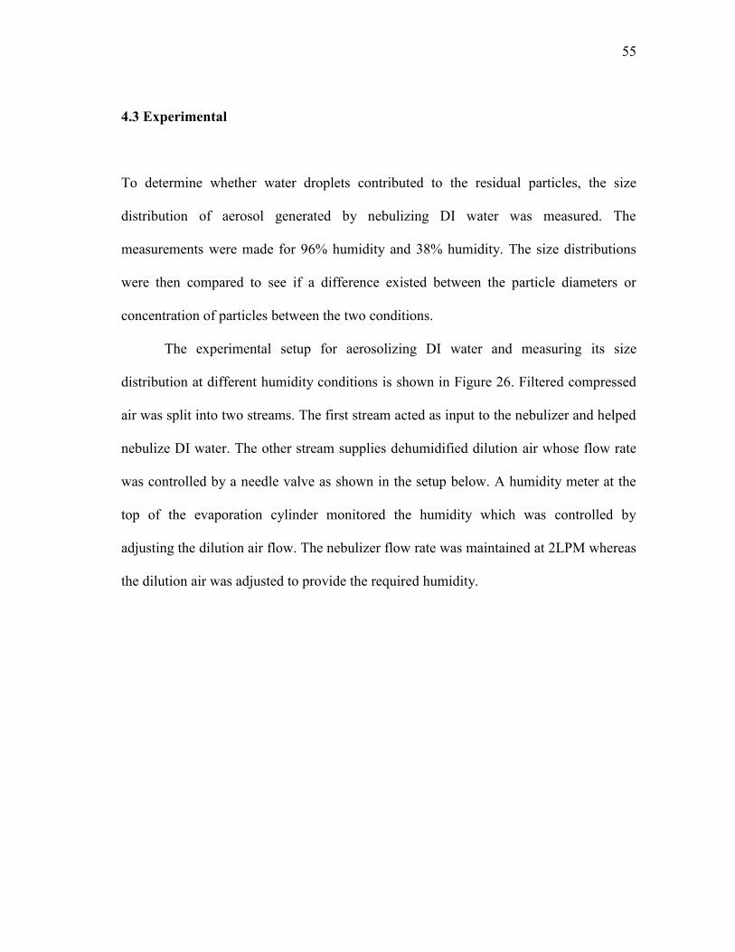
4.3 Experimental
To determine whether water droplets contributed to the residual particles, the size
distribution of aerosol generated by nebulizing DI water was measured. The
measurements were made for 96% humidity and 38% humidity. The size distributions
were then compared to see if a difference existed between the particle diameters or
concentration of particles between the two conditions.
The experimental setup for aerosolizing DI water and measuring its size
distribution at different humidity conditions is shown in Figure 26. Filtered compressed
air was split into two streams. The first stream acted as input to the nebulizer and helped
nebulize DI water. The other stream supplies dehumidified dilution air whose flow rate
was controlled by a needle valve as shown in the setup below. A humidity meter at the
top of the evaporation cylinder monitored the humidity which was controlled by
adjusting the dilution air flow. The nebulizer flow rate was maintained at 2LPM whereas
the dilution air was adjusted to provide the required humidity.
56
Figure 26: Experimental setup for measuring size distribution of DI water particles at different humidity conditions
Three experiments were performed for this study. In the first experiment, no
dilution air was provided and the evaporation cylinder was allowed to reach stable
condition. The relative humidity was thus observed to be approximately 96%. After this
stable condition was reached, a size distribution measurement was taken. In the second
experiment, the flow rate of dilution air was set to 4LPM which maintained a relative
humidity of 38% for exiting aerosol. To confirm that the particles resulted from
nebulization of DI water, the size distribution of particles in filtered air was measured.
This was done by removing DI water from the nebulizer jar and measuring the size
distribution of filtered air.
57
In the second part of the study, TEM analysis of particles collected using an
Electrostatic Precipitator was conducted. A diagram for the experimental apparatus for
collecting de-ionized water particles is shown in Figure 27. DI water was filled into the
nebulizer jar so that about 3/8” of the nozzle was below its surface.
Figure 27: Schematic of apparatus setup for collection of particles in de-ionized water
Two outlets were present at the top of the cylinder. One of the outlets was open
to the atmosphere and the aerosol flowed out through it at 1.70 LPM. The other outlet
was connected to a pump and a flow of 0.3LPM was maintained using a needle valve
upstream of the pump.
The aerosol passed through an Electrostatic Precipitator (ESP) in which de-
ionized water particles were collected upon a TEM grid. A voltage of -5000V was
applied on the high voltage terminal of the ESP while the other was connected to
58
ground. A corona discharge inside the ESP lead to collection of DI water particles on the
TEM grid which was later analyzed to determine the particle composition. A number of
samples were collected on the TEM grids for varying times, as it was difficult to
determine how much time it would take to collect enough particles for a detailed
analysis of size and chemical composition. Time periods included sampling for 1, 2, 3, 5,
20, and 60 minutes.
4.4 Results and Conclusions
Figure 28 shows the size distribution of residual particles for different humidity
conditions. A peak with approximately 37nm mode diameter was observed for the 96%
humidity condition. On the other hand, no such peak is observed for the size distribution
of particles for 38% humidity condition. This means that unevaporated water droplets
contribute to larger particles in the case where evaporation cylinder has a high humidity.
In the case of low humidity more droplets are able to evaporate and hence lower
concentration of residual particles. From the graph of filtered air used for dilution and
nebulization, it can be concluded that the residual particles observed are not from this
source.
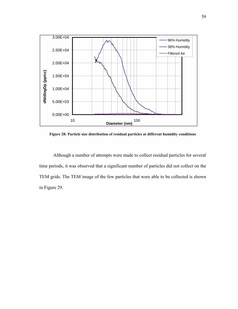
59
Figure 28: Particle size distribution of residual particles at different humidity conditions
Although a number of attempts were made to collect residual particles for several
time periods, it was observed that a significant number of particles did not collect on the
TEM grids. The TEM image of the few particles that were able to be collected is shown
in Figure 29.
0.00E+00
5.00E+03
1.00E+04
1.50E+04
2.00E+04
2.50E+04
3.00E+04
10 100
dN
/dlo
gD
p (
pp
/cc)
Diameter (nm)
96% Humidity
38% Humidity
Filtered Air
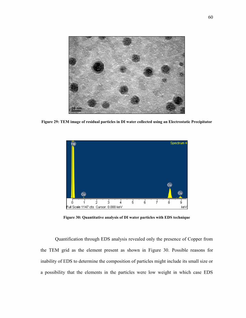
60
Figure 29: TEM image of residual particles in DI water collected using an Electrostatic Precipitator
Figure 30: Quantitative analysis of DI water particles with EDS technique
Quantification through EDS analysis revealed only the presence of Copper from
the TEM grid as the element present as shown in Figure 30. Possible reasons for
inability of EDS to determine the composition of particles might include its small size or
a possibility that the elements in the particles were low weight in which case EDS
61
technique is not very accurate. It can be concluded from this study that residual particles
observed during the aerosolization of suspensions of DI water were composed of
impurities present in DI water and unevaporated droplets of DI water. Although it was
possible to observe solid residual particles from aerosolization of DI water, EDS was not
able to determine the chemical composition of these particles.
62
5. SUMMARY
A Scanning Mobility Particle Spectrometer was designed using a Condensation Particle
Counter and a Differential Mobility Analyzer to measure the particle size distribution of
nanoparticles in an aerosol. It was built by accomplishing designs for hardware, which
consisted of the Electrical System and the Fluid Flow System, and the software.
Calibration of SEMS showed close similarity in the results of mode diameters obtained
from TEM analysis and SEMS. The mode diameter of 99nm nominal diameter PSL
particles was found to be 92.5 nm from TEM and 95.8nm from SEMS, a percentage
difference of 3.6%. Similarly, the mode diameter for 204nm was found to be 194.9nm
and 191.0nm from TEM and SEMS, respectively, a difference of 2.0%.
The SEMS was applied in the study of generation of TiO2 particles from Collison
nebulizer and residual particles in the aerosolization of de-ionized water. The Collison
nebulizer generated TiO2 particles with a mode diameter of 197.5nm, 200nm, and
195.2nm, respectively, for 3mM, 6mM and 9mM of TiO2 suspension which was higher
as compared to 95.0nm for the powder using TEM analysis. SEMS measurements
indicated a decreasing concentration of particles generated by the Collison nebulizer
with time and Dynamic Light Scattering technique confirmed agglomeration in the
suspension as the primary reason for increased mode diameter and decreasing
concentration of TiO2 aerosol. It was not possible to emulate single particle size
distribution by the use of surfactant, Tween 20, which only increased the concentration
of particles generated during the nebulizer run. Finally, by studying residual particles in

63
DI water, observed during the SEMS calibration process, it was found that the residual
particles are a mixture of solid impurity particles and unevaporated liquid droplets.
64
REFERENCES
Aitken, J. (1890). On a Simple Pocket Dust Counter, Proceedings of Royal Society of
Edinburgh, 39-54.
Baron, P. A. and Willeke, K. (2001). Aerosol Measurement: Principles, Techniques, and
Applications. Wiley, New York.
Charlesworth, D. H. and Marshall, W. R. (1960). Evaporation from Drops Containing
Dissolved Solids. Aiche J 6:9-23.
Colvin, V. L. (2003). The Potential Environmental Impact of Engineered Nanomaterials.
Nature Biotechnology 21:1166-1170.
Erikson, H. A. (1921). Change of Mobility of the Positive Ions in Air with Age. Physics
Review 18:100-101.
Flagan, R. C. (1998). History of Electrical Aerosol Measurements. Aerosol Science and
Technology 28:301-380.
Fuchs, N. A. (1963). On the Stationary Charge Distribution on Aerosol Particles in
Bipolar Ionic Atmosphere. Pure and Applied Geophysics 56:185-193.
Hinds, W. C. (1999). Aerosol Technology : Properties, Behavior, and Measurement of
Airborne Particles. Wiley, New York.
Hood, E. (2004). Nanotechnology: Looking as We Leap. Environmental Health
Perspectives 112:A740-A749.
65
Knutson, E. O. and Whitby, K. T. (1975). Aerosol Classification by Electric Mobility:
Apparatus, Theory and Applications. Aerosol Science and Technology 6:443-
451.
LaFranchi, B. W., Knight, M. and Petrucci, G. A. (2003). Leaching as a Source of
Residual Particles from Nebulization of Deionized Water. Journal of Aerosol
Science 34:1589-1594.
Navrotsky, A. (2000). Nanomaterials in the Environment, Agriculture, and Technology
(Neat). Journal of Nanoparticle Research 2:321-323.
Patist, A., Bhagwat, S. S., Penfield, K. W., Aikens, P. and Shah, D. O. (2000). On the
Measurement of Critical Micelle Concentrations of Pure and Technical-Grade
Nonionic Surfactants. J Surfactants Deterg 3:53-58.
Reich, D. H., Tanase, M., Hultgren, A., Bauer, L. A., Chen, C. S. and Meyer, G. J.
(2003). Biological Applications of Multifunctional Magnetic Nanowires
(Invited). Journal of Applied Physics 93:7275-7280.
Schick, M. J. (1967). Nonionic Surfactants. M. Dekker, New York,.
Schmoll, L. H., Elzey, S., Grassian, V. H. and O'Shaughnessy, P. T. (2009).
Nanoparticle Aerosol Generation Methods from Bulk Powders for Inhalation
Exposure Studies. Nanotoxicology 1.
Shimada, M., Wang, W. N., Okuyama, K., Myojo, T., Oyabu, T., Morimoto, Y., Tanaka,
I., Endoh, S., Uchida, K., Ehara, K., Sakurai, H., Yamamoto, K. and Nakanishi,
J. (2009). Development and Evaluation of an Aerosol Generation and Supplying
66
System for Inhalation Experiments of Manufactured Nanoparticles.
Environmental Science & Technology 43:5529-5534.
Wang, S. C. and Flagan, R. C. (1990). Scanning Electrical Mobility Spectrometer.
Aerosol Science and Technology 13:230-240.
Wiedensohler, A. (1988). An Approximation of the Bipolar Charge-Distribution for
Particles in the Sub-Micron Size Range. Journal of Aerosol Science 19:387-389.
Zahn, M. (2001). Magnetic Fluid and Nanoparticle Applications to Nanotechnology.
Journal of Nanoparticle Research 3:73-78.
Zhang, S. H., Akutsu, Y., Russell, L. M., Flagan, R. C. and Seinfeld, J. H. (1995). Radial
Differential Mobility Analyzer. Aerosol Science and Technology 23:357-372.
Zhao, B., Yang, Z. W., Wang, J. J., Johnston, M. V. and Wang, H. (2003). Analysis of
Soot Nanoparticles in a Laminar Premixed Ethylene Flame by Scanning Mobility
Particle Sizer. Aerosol Science and Technology 37:611-620.
Zhu, Y. F., Hinds, W. C., Kim, S. and Sioutas, C. (2002). Concentration and Size
Distribution of Ultrafine Particles Near a Major Highway. J Air Waste Manage
52:1032-1042.
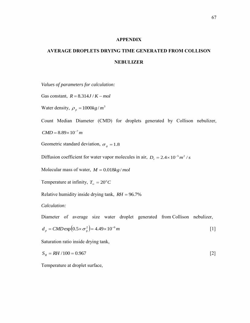
67
APPENDIX
AVERAGE DROPLETS DRYING TIME GENERATED FROM COLLISON
NEBULIZER
Values of parameters for calculation:
Gas constant, molKJR /314.8
Water density, 3/1000 mkgp
Count Median Diameter (CMD) for droplets generated by Collison nebulizer,
mCMD 71089.8
Geometric standard deviation, 8.1g
Diffusion coefficient for water vapor molecules in air, smDv /104.2 25
Molecular mass of water, molkgM /018.0
Temperature at infinity, CT o20
Relative humidity inside drying tank, %7.96RH
Calculation:
Diameter of average size water droplet generated from Collison nebulizer,
mCMDd gp
62 1049.45.0exp [1]
Saturation ratio inside drying tank,
967.0100/ RHSR [2]
Temperature at droplet surface,
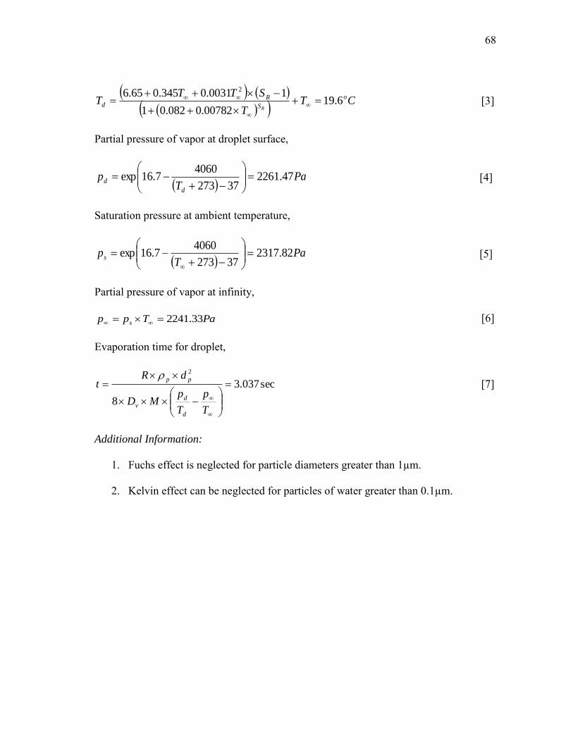
68
CT
T
STTT o
S
Rd
R
6.1900782.0082.01
10031.0345.065.6 2
[3]
Partial pressure of vapor at droplet surface,
Pa
Tp
d
d 47.226137273
40607.16exp
[4]
Saturation pressure at ambient temperature,
Pa
Tps 82.2317
37273
40607.16exp
[5]
Partial pressure of vapor at infinity,
PaTpp s 33.2241 [6]
Evaporation time for droplet,
sec037.3
8
2
T
p
T
pMD
dRt
d
dv
pp [7]
Additional Information:
1. Fuchs effect is neglected for particle diameters greater than 1µm.
2. Kelvin effect can be neglected for particles of water greater than 0.1µm.
69
VITA
Name: Gagan Singh
Address: Department of Mechanical Engineering, Texas A&M University, 3123 TAMU, College Station, TX 77843-3123, USA Email Address: [email protected] Education: B.S., Mechanical Engineering, Texas A&M University, 2006 M.S., Mechanical Engineering, Texas A&M University, 2010