DESIGN OF CLOSED LOOP SYSTEMS

USING COMPENSATION TECHNIQUES

IN TIME DOMAIN

Lecture Outline

• Introduction to Lead Compensation

• Electronic Lead Compensator

• Electrical Lead Compensator

• Mechanical Lead Compensator

Lead Compensation

• Lead Compensation essentially yields an appreciable improvement in transient response and a small change in steady state accuracy.

• There are many ways to realize lead compensators and lag compensators, such as electronic networks using operational amplifiers, electrical RC networks, and mechanical spring-dashpot systems.

Lead Compensation

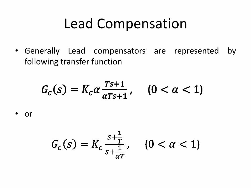
• Generally Lead compensators are represented by following transfer function

• or

Lead Compensation

-10 -8 -6 -4 -2 0-1

-0.5

0

0.5

1

Pole-Zero Map

Real Axis

Imagin

ary

Axis

-20

-15

-10

-5

0

Magnitu

de (

dB

)

10-2

10-1

100

101

102

103

0

30

60

Phase (

deg)

Bode Diagram

Frequency (rad/sec)

Electronic Lead Compensator

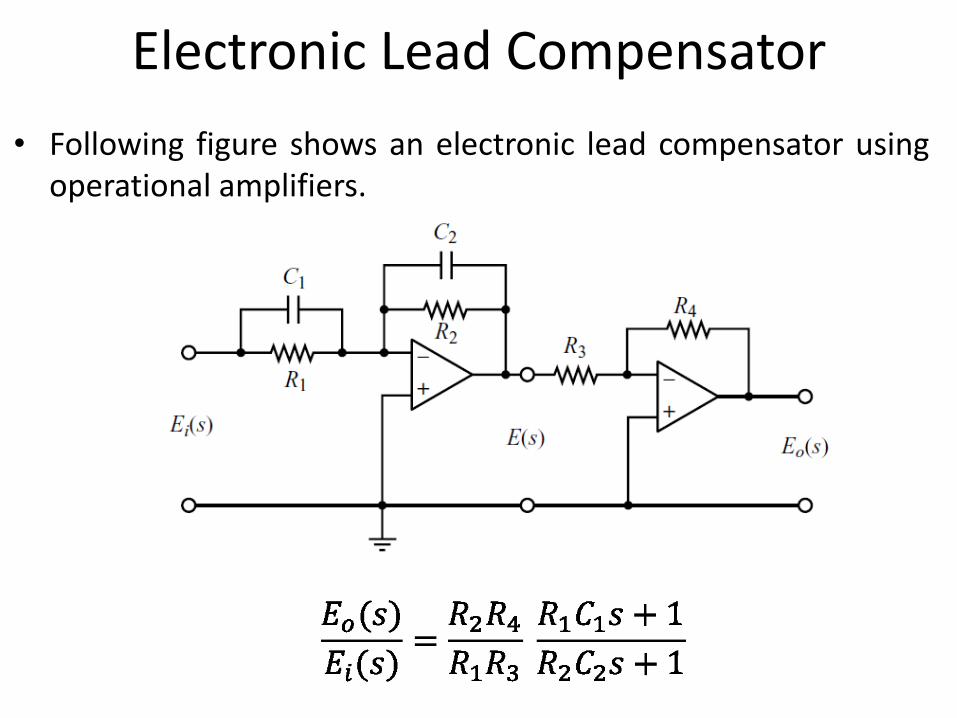
• Following figure shows an electronic lead compensator using operational amplifiers.

Electronic Lead Compensator

Electronic Lead Compensator

• Pole-zero Configuration of Lead Compensator

Lead Compensation Techniques Based on the Root-Locus Approach.

• The root-locus approach to design is very powerful when the specifications are given in terms of time-domain quantities, such as

– damping ratio

– undamped natural frequency

– desired dominant closed-loop poles

– maximum overshoot

– rise time

– settling time.

Lead Compensation Techniques Based on the Root-Locus Approach.

• The procedures for designing a lead compensator by the root-locus method may be stated as follows:

– Step-1: Analyze the given system via root locus.

Step-2

• From the performance specifications, determine the desired location for the dominant closed-loop poles.

Step-3

• From the root-locus plot of the uncompensated system (original system), ascertain whether or not the gain adjustment alone can yield the desired closed loop poles.

• If not, calculate the angle deficiency.

• This angle must be contributed by the lead compensator if the new root locus is to pass through the desired locations for the dominant closed-loop poles.

Step-4

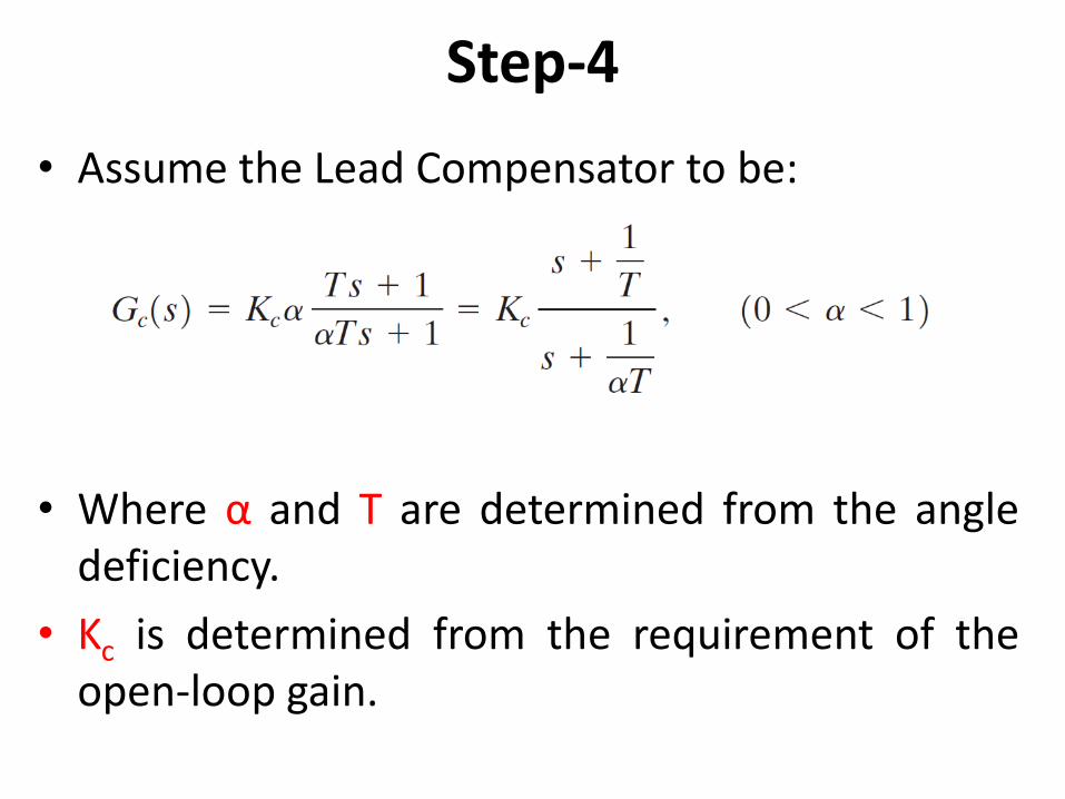
• Assume the Lead Compensator to be:

• Where α and T are determined from the angle deficiency.

• Kc is determined from the requirement of the open-loop gain.

Step-5

• If static error constants are not specified, determine the location of the pole and zero of the lead compensator so that the lead compensator will contribute the necessary angle.

• If no other requirements are imposed on the system, try to make the value of α as large as possible.

• A larger value of α generally results in a larger value of Kv, which is desirable.

• Larger value of α will produce a larger value of Kv and in most cases, the larger the Kv is, the better the system performance.

Step-6

• Determine the value of Kc of the lead compensator from the magnitude condition.

Final Design check

• Once a compensator has been designed, check to see whether all performance specifications have been met.

• If the compensated system does not meet the performance specifications, then repeat the design procedure by adjusting the compensator pole and zero until all such specifications are met.

Final Design check

• If the selected dominant closed-loop poles are not really dominant, or if the selected dominant closed-loop poles do not yield the desired result, it will be necessary to modify the location of the pair of such selected dominant closed-loop poles.

Example-1

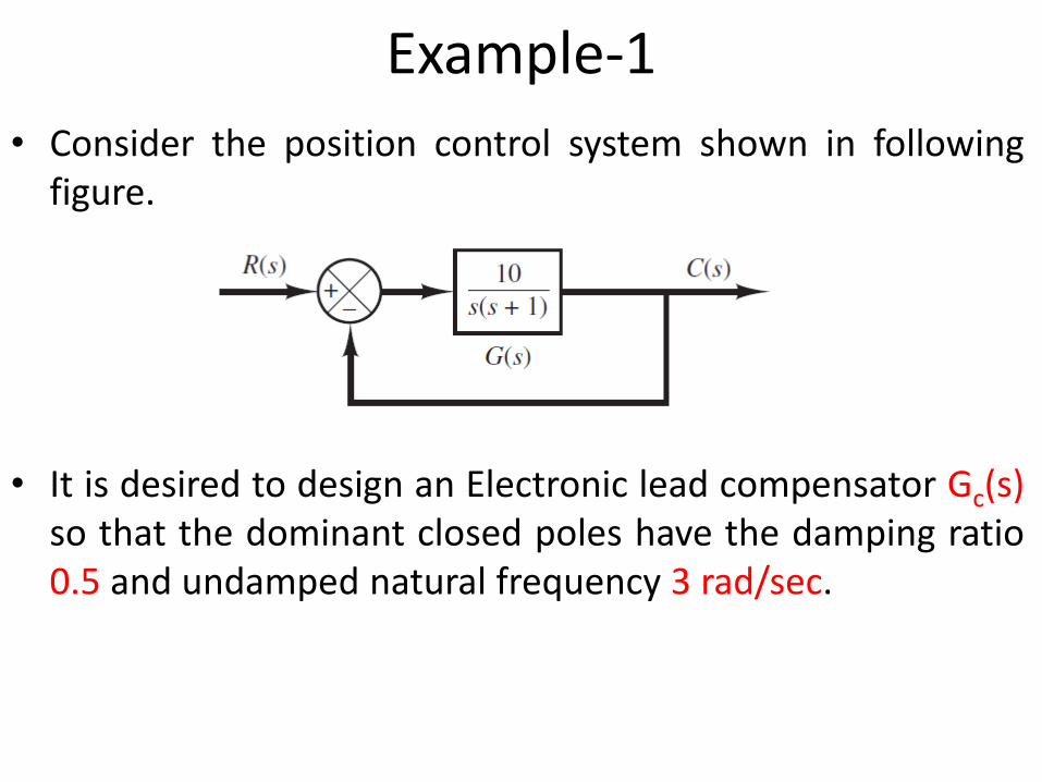
• Consider the position control system shown in following figure.

• It is desired to design an Electronic lead compensator Gc(s) so that the dominant closed poles have the damping ratio 0.5 and undamped natural frequency 3 rad/sec.

Step-1 (Example-1)

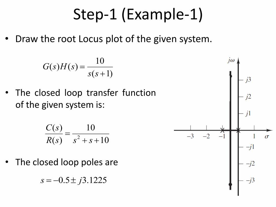
• Draw the root Locus plot of the given system.

)1(

10)()(

sssHsG

• The closed loop transfer function of the given system is:

• The closed loop poles are

10

10

)(

)(2

sssR

sC

1225.35.0 js

Step-1 (Example-1)

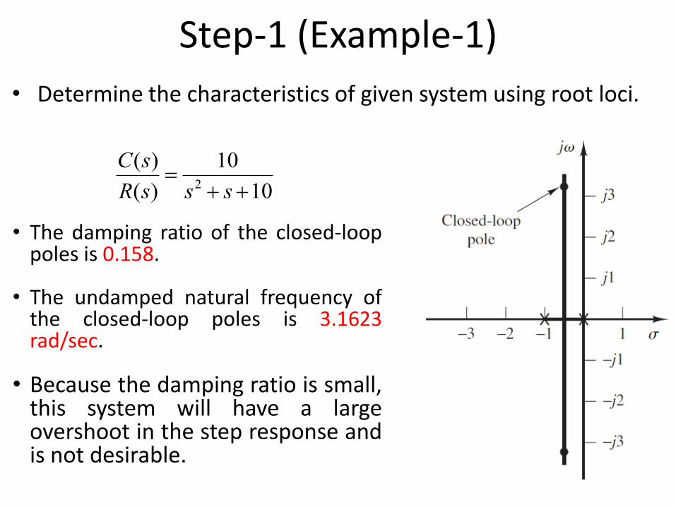
• Determine the characteristics of given system using root loci.

• The damping ratio of the closed-loop poles is 0.158.

• The undamped natural frequency of the closed-loop poles is 3.1623 rad/sec.

• Because the damping ratio is small, this system will have a large overshoot in the step response and is not desirable.

10

10

)(

)(2

sssR

sC

Step-2 (Example-1)

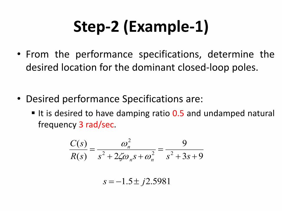
• From the performance specifications, determine the desired location for the dominant closed-loop poles.

• Desired performance Specifications are:

It is desired to have damping ratio 0.5 and undamped natural frequency 3 rad/sec.

93

9

2)(

)(222

2

sssssR

sC

nn

n

5981.25.1 js

Step-2 (Example-1)

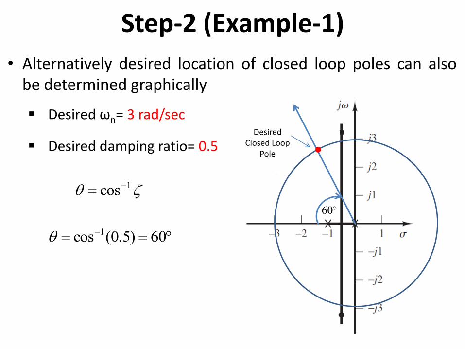
• Alternatively desired location of closed loop poles can also be determined graphically

Desired ωn= 3 rad/sec

Desired damping ratio= 0.5

1cos

60)5.0(cos 1

Desired Closed Loop

Pole

60

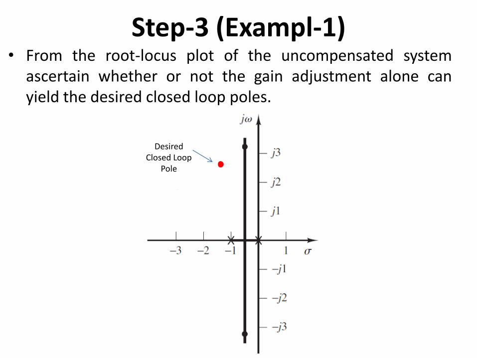
Step-3 (Exampl-1) • From the root-locus plot of the uncompensated system

ascertain whether or not the gain adjustment alone can yield the desired closed loop poles.

Desired Closed Loop

Pole

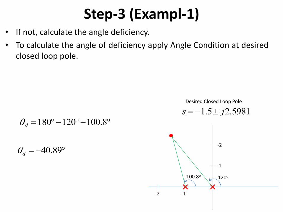
Step-3 (Exampl-1) • If not, calculate the angle deficiency.

• To calculate the angle of deficiency apply Angle Condition at desired closed loop pole.

-1

5981.25.1 js

Desired Closed Loop Pole

-1

-2

-2

120o 100.8o

8.100120180d

89.40d

Step-3 (Exampl-1)

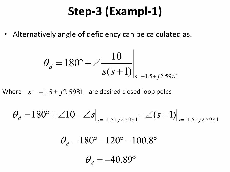
• Alternatively angle of deficiency can be calculated as.

5981.25.1 js Where are desired closed loop poles

5981.25.1)1(

10180

js

dss

5981.25.15981.25.1)1(10180

jsjsd ss

8.100120180d

89.40d

Step-4 (Exampl-1)

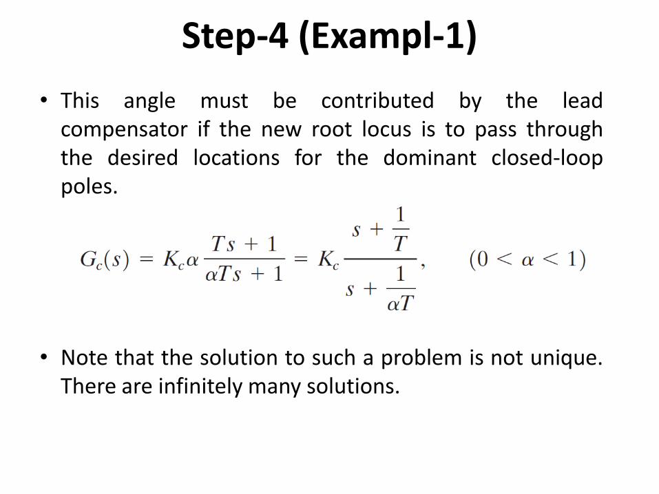
• This angle must be contributed by the lead compensator if the new root locus is to pass through the desired locations for the dominant closed-loop poles.

• Note that the solution to such a problem is not unique. There are infinitely many solutions.

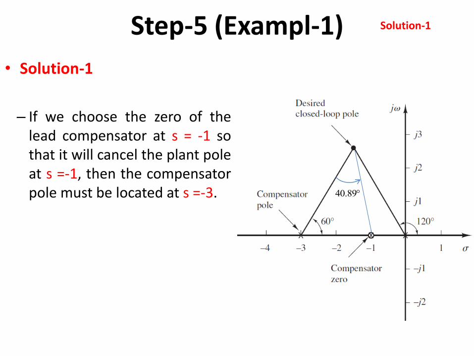
Step-5 (Exampl-1)

• Solution-1

– If we choose the zero of the lead compensator at s = -1 so that it will cancel the plant pole at s =-1, then the compensator pole must be located at s =-3. 89.40

Solution-1