ARTICLE IN PRESS

Neurocomputing 72 (2009) 1160– 1178

Contents lists available at ScienceDirect

Neurocomputing

0925-23

doi:10.1

� Corr

E-m

journal homepage: www.elsevier.com/locate/neucom

Design of experiments on neural network’s training for nonlineartime series forecasting

P.P. Balestrassi a,�, E. Popova b, A.P. Paiva a, J.W. Marangon Lima a

a Federal University of Itajuba, Brazilb University of Texas at Austin, USA

a r t i c l e i n f o

Article history:

Received 10 August 2007

Received in revised form

9 February 2008

Accepted 20 February 2008

Communicated by T. Heskestime series—that is related to many real problems such as short-term electricity loads, daily prices and

Available online 29 February 2008

Keywords:

Design of Experiment

Artificial Neural Network

Nonlinear time series

12/$ - see front matter & 2008 Elsevier B.V. A

016/j.neucom.2008.02.002

esponding author. Tel.: +55 3591198924.

ail address: pedro@unifei.edu.br (P.P. Balestra

a b s t r a c t

In this study, the statistical methodology of Design of Experiments (DOE) was applied to better

determine the parameters of an Artificial Neural Network (ANN) in a problem of nonlinear time series

forecasting. Instead of the most common trial and error technique for the ANN’s training, DOE was

found to be a better methodology. The main motivation for this study was to forecast seasonal nonlinear

returns, water consumption, etc. A case study adopting this framework is presented for six time series

representing the electricity load for industrial consumers of a production company in Brazil.

& 2008 Elsevier B.V. All rights reserved.

1. Introduction

DOE is considered one of the most important methodologiesfor researchers who deal with experiments in practical applica-tions, with a huge amount of success stories. Nowadays, DOEresources are incorporated in many statistical software packagesthat ease calculation and interpretation of results [8]. Similarly,ANNs play an important role for problems of time seriesforecasting [19]. One often quoted drawback in using ANNs,however, is the optimization of the ANN’s parameters. In general,the lengthy trial-and-error process is what most practitioners usefor this optimization [63].

The main motivation for this work is to forecast nonlinear andseasonal time series—which is a real problem for many applica-tions—using ANN. Usually daily, monthly, or yearly seasonality isinherent to several problems related to prices, returns, electricityload, water consumption, demand, etc. Nonlinear structures arealso present in most cases. DOE is here used to estimate theparameters of an ANN through simulation.

There is a lack of literature on this specific issue and somequestions are subject to investigation. Among others, the follow-ing questions will be addressed in this paper: How to approach

problems of nonlinear seasonal time series using ANNs? How to train

ANNs for this kind of problem? How many factors are important to

this approach? Are there interactions that should be considered?

ll rights reserved.

ssi).

This paper describes in Section 2 the recent literature review ofDOE on ANNs for problems of nonlinear time series forecasting.Section 3 presents numerical and graphical results for the overallprocedure. Section 4 presents a case study for short-termelectricity load problem using the DOE on ANN’s framework.Section 5 states our main conclusions.

2. Background and literature review

2.1. Design of experiments for simulation

The process of training an ANN consists in changing the inputparameters of a computational algorithm, running the algorithm,and checking the results. This can be referred as a simulationstudy for the ANN problem.

In spite of the amount of success stories related to industrialapplications, DOE is not used as widely in simulation as it should be.Kleijnen et al. [34] points that the lack of use of DOE for simulationis due to some reasons: (i) Simulation analysts are not convinced ofthe benefits of DOE. (ii) DOE research is often found in specialtyjournals seldom read by simulation analysts. (iii) Most DOEs wereoriginally developed for real-world experimentation rather thandeveloped specifically for simulation settings. The aforementionedresearch also points the main benefits of experimental design onmodel development and simulation and predicts that the use ofDOE is likely to become more substantial in this area:

DOE can uncover detailed insight into the model’s behavior,cause the modeling team to discuss in detail the implications

ARTICLE IN PRESS

Fig. 1. Multilayer feedforward ANN structure.

P.P. Balestrassi et al. / Neurocomputing 72 (2009) 1160–1178 1161

of various model assumptions, help frame questions when theanalysts may not know ahead of time what questions shouldbe asked, challenge or confirm expectations about the direc-tion and relative importance of factor effects, and even uncoverproblems in the program logic y Design suited to a particularapplication is much better than trial and error or a simple,small design. Consequently, practitioners should be open to thenotion that DOE is a useful and necessary part of analysis ofcomplex simulation.

Translating the simulation terminology it could be said that aninput or a parameter in simulation is referred to as a factor in DOE.Usually there are many more factors in simulation than in a real-world experiment. A factor can be either qualitative or quantita-

tive. Each factor can be set to two or more values, called factor

levels, typically coded numerically for analysis purposes. Ascenario or design point is a combination of levels for all factors.In considering stochastic simulations replicates mean that differ-ent Pseudo-Random Numbers (PRNs) are used to simulate thesame scenario. The nature of the data collection of scenarios is notrandom but sequential. Unless otherwise specified, it is assumedthat replicates use nonoverlapping PRN streams, so outputs acrossreplicates are Independently Identically Distributed (IID)—as moststatistical methods assume. Developing a basic understanding insimulation is referred as testing hypotheses about factor effects

in DOE [34].Another important issue when using DOE for simulation is that

the main goal here is not optimization. In using DOE the effortsare dedicated to find robust policies or decisions, rather thanoptimal policies. It is certainly true that finding the optimal policyfor a simulated system is a hot topic, and many methods havebeen proposed. Fu [18] and Spall [50] discuss the current researchand practice of optimization for simulation. These methodsinclude heuristic search techniques—such as genetic algorithms,response surface methodology (RSM), simulated annealing, tabusearch—and methods that analyze the simulation model toestimate gradients—such as perturbation analysis and scorefunctions. The result of the ‘‘optimization’’ is conditioned onassumptions of specific (typically assumed independent) distribu-tions and many input variables. The term ‘‘optimum’’ is proble-matic when the probability of all these assumptions holding inpractice—even for a limited time—is effectively zero. In contrast,a robust design approach treats all these assumptions asadditional factors when running the experiment. These areconsidered noise factors (rather than decision factors) becausethey are unknown or uncontrollable in the real-world environ-ment. A robust system or policy works well across a range of noiseconditions that might be experienced, so implementing a robustsolution is much less likely to result in unanticipated results. Thisrobust design philosophy is inspired by Taguchi [65], who usessimple designs to identify robust product configurations forToyota.

2.2. Artificial Neural Networks for problems of time series forecasting

ANNs, first used in the fields of cognitive science andengineering, are universal and highly flexible function approx-imators. As cited by Tsay [56], ANNs are general and flexible toolsfor forecasting applications:

A popular topic in modern data analysis is ANN, which can beclassified as a semiparametric method. As opposed to themodel-based nonlinear methods, ANNs are data-driven ap-proaches which can capture nonlinear data structures withoutprior assumption about the underlying relationship in aparticular problem.

Fig. 1 shows the ANN structure employed in the present study:A multilayer feedforward network trained with Backpropagation.The ANN has three types of layers, namely, the input layer, theoutput layer and the hidden layer, which is intermediate betweenthe input and output layers. The number of hidden layers isusually 1 or 2. Each layer consists of neurons, and the neurons intwo adjacent layers are fully connected with respective weights,while the neurons within the same layer are not connected. In thispaper, the output layer has just a single neuron, which representsthe one-step forecasting based on previous points.

Each neuron in the input layer is designated to an attribute inthe data, and produces an output which is equal to the (scaled)value of the corresponding attribute. For each neuron in thehidden or output layer, the following input–output transformationis employed:

v ¼ fXH

h¼1

whuh þw0

!,

where v is the output, H is the total number of neurons in theprevious layer, uh is the output of the hth neuron in the previouslayer, wh is the corresponding connection weight, w0 is the bias(or intercept). f is the nonlinear transformation function (oractivation function) also used in the output layer. The followingtransformation function, as example, is employed very often:

f ðzÞ ¼2

ð1þ e�zÞ� 1.

When the ANN is trained using the Backpropagation algorithmthe weights and biases are optimized. The objective functionemployed for optimization is the sum of the squares of thedifference between a desirable output (ytarget) and an estimatedoutput (ybpn).

Review of ANNs from statistical and econometric perspectivescan be found in [11]. Today, ANNs are used in a variety of modelingand forecasting problems. Although many models commonly usedin real problems are linear, the nature of most real data setssuggests that nonlinear problems are more appropriate forforecasting and accurately describing it. ANN plays an importantrole for this kind of forecasting.

The literature on ANN is enormous and its applications spreadover many scientific areas with varying degrees of success. In theM-Competition [39], M2-Competition [40] and M3-Competition[38] many participants used ANNs. The main reason for thisincreased popularity of ANNs is that these models have beenshown to be able to approximate almost any nonlinear functionarbitrarily close. Hence, when applied to a time series which ischaracterized by truly nonlinear dynamic relationships, the ANNwill detect these and provide a superior fit compared to linearmodels, without the need to construct a specific parametricnonlinear time series model.

ARTICLE IN PRESS

P.P. Balestrassi et al. / Neurocomputing 72 (2009) 1160–11781162

Addressing the problem of time series forecasting, someimportant papers have considered ANNs as a promising metho-dology and addressed important issues. Franses and van Homelen[17] explore the ability of ANNs to capture nonlinearity as impliedby SETAR, Markov-Switching and GARCH models. Kaastra andBoyd [28] provide an introductory guide—an eight-step procedur-e—in the design of a neural network for forecasting economictime series data. Bodyanskiy and Popov [66] present a special ANNapproach to forecasting financial time series based on thepresentation of the series as a combination of quasi-periodiccomponents. Tseng et al. [57] proposes a hybrid forecastingmodel, which combines the seasonal time series ARIMA (SARIMA)and the neural network Backpropagation (BP) models, namedthere as SARIMABP. Karunasinghe and Liong [30] investigate theperformance of ANNs as a global model over the widely used localmodels (local averaging technique and local polynomials techni-que) in chaotic time series. In the paper of Aitkenhead et al. [1],oil, stream water, and climatic variables, were measured hourlyover several month periods in two situations in North-East (NE)Scotland, using data loggers and other measuring instruments.The data sets were used to train neural networks using threedifferent methods, including a novel, biologically plausiblesystem. BuHamra et al. [7] combine the Box–Jenkins (BJ) andthe ANN approaches to model time series data of waterconsumption in Kuwait. Shi et al. [49] investigate nonlinear timeseries modeling using the general state-dependent autoregressivemodel. Niska et al. [43] model the air quality using ANN, a difficulttask due to both their chaotic and nonlinear phenomenon andhigh dimensional sample space. Zhang [61] presents a hybridmethodology that combines both ARIMA model and ANNs to takeadvantage of the unique strength of ARIMA model and ANNs inlinear and nonlinear modeling. Kim [32] uses support vectormachines (SVMs) for the prediction of financial time series. Thisstudy applies SVM to predicting the stock price index. Ho et al.[23] show a comparative study of ANN and ARIMA modeling intime series prediction. BP and Recurrent ANN gives satisfactoryperformance compared to ARIMA. Kohzadi et al. [35] compareARIMA and ANN price forecasting performance. Terasvirta et al.[54] examine the forecast accuracy of linear autoregressive,smooth transition autoregressive (STAR), and ANNs for 47monthly macroeconomic variables of the G7 economies. Ghiassiet al. [19] present a dynamic neural network model for forecastingtime series events that uses a different architecture thantraditional models. Balkin and Ord [3] explain a method, calledAutomated ANNs, that is an attempt to develop an automaticprocedure for selecting the architecture of an Artificial NeuralNetwork for forecasting purposes. Cubiles-de-la-Vega et al. [67]propose a procedure for designing a multilayer perceptron forpredicting time series. It is based on the generation, according to aset of rules emerging from an ARIMA model previously fitted, of aset of nonlinear forecasting models. Kalaitzakis et al. [29] presentthe development and application of advanced neural networks toface successfully the problem of the short-term electric loadforecasting, using actual hourly load data from the power systemof the island of Crete, in Greece. Qi and Zhang [46] exposeproblems of the commonly used information-based in-samplemodel selection criteria in selecting ANNs for financial time seriesforecasting. Zhang and Qi [62] investigate the problem ofseasonality and show that limited empirical studies on seasonaltime series forecasting with neural networks yield mixed results.In Chiang et al. [12], it was reported that the ANN proved to besuperior to regression models when the data availability islimited, e.g., newly launched mutual funds which have limitedhistorical data.

This research is partially motivated by the results presented inthe following papers. Zhang [60], examining the capability of ANN

for linear time series using both simulated and real data, statesthat ANN is quite competent in modeling and forecasting lineartime series in a variety of situations and simple neural structuresare often effective. Hwarng and Ang [27] and Hwarng [26] mainlymotivated by linear time series forecasting addresses some ideasthat are relevant for the present work: (i) ‘‘BackpropagationNeural Networks (BPNNs) generally performed well and consis-tently for time series corresponding to ARMA(p, q) structures,mainly when a particular noise level was considered during thenetwork training’’. (ii) ‘‘Given the well notion that multilayerfeedforward NN may act as a universal approximators, it isreasonable to expect that BPNNs can perform at least comparablyon linear data. If so, one may find it convenient to apply BPNNsregardless of the nature of data especially when the functionalform of data is unknown’’. Zhang et al. [63] present a compre-hensible state of the art survey of ANN applications in time seriesforecasting for the past decade and the following points are hereconsidered: (i) ‘‘Overall, ANNs give satisfactory performance inforecasting’’. (ii) ‘‘There are many factors that can affect theperformance of ANNs. However, there are no systematic investi-gations of these issues. The shot-gun (trial and error) methodol-ogy for specific problems is typically adopted by most researchers,which is the primary reason for inconsistencies in the literature’’.(iii) ‘‘A considerable amount of research has been done in this areagiven the fast-growing nature of the literature’’.

2.3. Nonlinear time series

Linear time series methods have been used widely for the pasttwo decades. Recently, however, there has been increasing interestin extending the classical framework of Box and Jenkins [5] toincorporate nonstandard properties, such as nonlinearity, non-Gaussianity, and heterogeneity. In this way, a great number ofnonlinear models have been developed, such as the bilinear modelof Granger and Anderson [20], the threshold autoregressive (TAR)model of Tong [55], the state-dependent model of Priestley [45],the Markov switching model of Hamilton [22], the functional-coefficient autoregressive model of Chen and Tsay [10], amongmany others. Although the properties of these models tend tooverlap somewhat, each is able to capture a wide variety ofnonlinear behavior. In most time series, however, this kind ofmodeling is even more complex due to some features like highfrequency, daily and weekly seasonality, calendar effect onweekend and holidays, high volatility and presence of outliers.In particular, it has been shown that the ANN model is able toapproximate any well-behaved nonlinear relationship to anarbitrary degree of accuracy, in much the same way that anARMA model provides a good approximation of general linearrelationships [9,24]. This is the so-called universal approximation

property of ANNs. In short, feedforward ANN with a hidden layercan be seen as a way to parameterize a general continuousnonlinear function.

The problem one immediately faces when considering the useof nonlinear time series models is the vast, if not unlimited,number of possible models. Consider a univariate time series xt

which for simplicity is observed at equally spaced time points. Wedenote the observations by {xt|t ¼ 1,y,T}, where T is the samplesize. A purely stochastic time series xt is said to be linear if it canbe written as

xt ¼ mþX1i¼0

ciat�i,

where m is a constant, ci are real numbers with c0 ¼ 1, and {at} is asequence of independent and identically distributed (IID) randomvariables with a well-defined distribution function. We assume

ARTICLE IN PRESS

P.P. Balestrassi et al. / Neurocomputing 72 (2009) 1160–1178 1163

that the distribution of at is continuous and E(at) ¼ 0. In manycases, we further assume that VarðatÞ ¼ s2

a or, even stronger, thatat is Gaussian. If s2

a

P1i¼1c

2i o1 then xt is weakly stationary (i.e.,

the first two moments of xt are time-invariant). The ARMA processis linear because it has an MA representation in the mentionedequation. Any stochastic process that does not satisfy thecondition of this equation is said to be nonlinear. See [56] formore details. For previous and more general surveys on nonlineartime series models, the interested reader is referred to [55,21].

A natural approach to modeling time series with nonlinearmodels seems to define different states of the world or regimes, andto allow for the possibility that the dynamic behavior of variablesdepends on the regime that occurs at any given point in time [45].By state-dependent dynamic behavior of a time series it is meantthat certain properties of the time series, such as its mean,variance and/or autocorrelation, are different in different regimes.In particular, autocorrelations tend to be larger during periods oflow volatility and smaller during periods of high volatility. Theperiods of low and high volatility can be interpreted as differentregimes. Of course, the level of volatility in the future is notknown with certainty. The best one can do is to make a sensibleforecast of this level and, hence, of the regime that will occur inthe future [36]. The state-dependent, or regime-switching con-siders that the regime is stochastic and not deterministic, witch isrelevant for many time series. There are two main classes ofregime-switching models: (i) Regimes determined by observablevariables that include the Bilinear model, the TAR (ThresholdAutoregressive) model and the SETAR (Self-Exciting ThresholdAutoregressive) model and (ii) Regimes determined by unobser-vable variables that include the MSW (Markov-Switching) model.We restrict our attention to models that assume that in each ofthe regimes the dynamical behavior of the time series is modeledwith an AR model. In other words, the time series is modeled withan AR model, where the autoregressive parameters are allowed todepend on the regime or state. Generalizations of the MA model toa regime-switching context have also been considered [13], butwe abstain from discussing these models here.

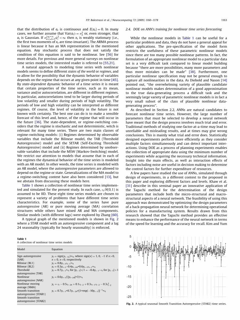
Table 1 shows a collection of nonlinear time series implemen-ted and simulated for the present study. In each case, et:N(0,1) isassumed to be IID. These eight time series models are chosen torepresent a variety of problems that have different time seriescharacteristics. For example, some of the series have pureautoregressive (AR) or pure moving average (MA) correlationstructures while others have mixed AR and MA components.Similar models (with different lags) were explored by Zhang [60].

A typical graph of the mentioned models is shown in Fig. 2where a STAR model with an autoregressive component and a lag24 seasonality (typically for hourly seasonality) is enforced.

Table 1A collection of nonlinear time series models

Model Equation

Sign autoregressive

(SAR)

yt ¼ sign(yt�12)+et, where sign(x) ¼ 1, 0, �1 if x40,

x ¼ 0, xo0, respectively

Bilinear (BL1) yt ¼ 0.8yt�1et�1+et

Bilinear (BL2) yt ¼ 0.3yt�1�0.4yt�24+0.6yt�1et�1+et

Threshold

autoregressive (TAR)

yt ¼ 0.7yt�1+et for |yt�1|p1 ¼ �0.4yt�1�et for |yt�1|41

Nonlinear

autoregressive (NAR)

yt ¼ 0.6yt�1/(|yt�24|+3)+et

Nonlinear moving

average (NMA)yt ¼ �t � 0:5�t�24 þ 0:1�t�2 þ 0:3�t�1�t�2 � 0:3�2t�2

Smooth transition

autoregressive (STAR1)

yt ¼ 0.7yt�1+0.7yt�24+[1+exp(�10yt�1)]�1+et

Smooth transition

autoregressive (STAR2)

2.4. DOE on ANN’s training for nonlinear time series forecasting

While the nonlinear models in Table 1 can be useful for aparticular problem and data, they do not have a general appeal forother applications. The pre-specification of the model formrestricts the usefulness of these parametric nonlinear modelssince there are too many possible nonlinear patterns. In fact, theformulation of an appropriate nonlinear model to a particular dataset is a very difficult task compared to linear model buildingbecause ‘‘there are more possibilities, many more parameters andthus more mistakes can be made’’ [38]. Furthermore, oneparticular nonlinear specification may not be general enough tocapture all nonlinearities in the data. As Diebold and Nason [14]pointed out, ‘‘the overwhelming variety of plausible candidatenonlinear models makes determination of a good approximationto the true data-generating process a difficult task and theseemingly large variety of parametric nonlinear models is in fact avery small subset of the class of plausible nonlinear data-generating process’’.

As described in Section 2.2, ANNs are natural candidates toforecast nonlinear time series. However, the large number ofparameters that must be selected to develop a neural networkhave meant that the design process involves much trial and error.Traditional methods of studying one-factor-at-a-time may lead tounreliable and misleading results, and at times may give wrongconclusions. This is mainly what trial and error does. Statisticallydesigned experiments perform more efficiently as they considermultiple factors simultaneously and can detect important inter-actions. Using DOE as a process of planning experiments enablesthe collection of appropriate data using the minimum number ofexperiments while acquiring the necessary technical information.Insight into the main effects, as well as interaction effects offactors including noise are useful in decision making to determinethe control factors for further expenditure of resources.

A few papers have studied the use of ANNs, simulated throughdesign of experiments, in a different context to the proposed inthis paper and exploring different factors and levels. Khaw et al.[31] describe in this seminal paper an innovative application ofthe Taguchi method for the determination of the designparameters that include both the micro-structural and macro-structural aspects of a neural network. The feasibility of using thisapproach was demonstrated by optimizing the design parametersof a back-propagation neural network for determining operationalpolicies for a manufacturing system. Results drawn from thisresearch showed that the Taguchi method provides an effectivemeans to enhance the performance of the neural network in termsof the speed for learning and the accuracy for recall. Kim and Yum

-25

-20

-15

-10

-5

0

5

Fig. 2. A typical seasonal Smooth Transition Autoregressive (STAR2) time series.

ARTICLE IN PRESS

P.P. Balestrassi et al. / Neurocomputing 72 (2009) 1160–11781164

[33] present a similar paper. Sukthomya and Tannock [52,53] usethe same Taguchi experimental design idea to set the parametersof an ANN in a complex forming process. Lin and Tseng [37] alsouse the same Taguchi approach for a ‘‘Learning Vector Quantiza-tion’’ ANN on an application to bicycle derailleur systems.Enemuoh and El-Gizawy [16] describe a method for robust designof an ANN for prediction of delamination, damage width, and holesurface roughness during drilling in carbon fiber reinforced epoxy.The effects of number of neurons, hidden layers, activationfunction, and learning algorithm on the mean square error ofmodel prediction are quantified. Using the aforementionedmethod, a robust ANN was developed that predicted process-induced damage with high accuracy. Zhang [60] and Zhang et al.[64] present an experimental evaluation of neural networks forlinear and nonlinear time series forecasting. Three main ANNparameters are examined through a simulated computer experi-ment: input nodes, hidden nodes and sample size. The modelsused in these papers were similarly reproduced in the presentwork (see Table 2) for comparative purposes.

When compared with the previous papers, the present studycould be mainly innovative in the following points:

�

Instead of using the Taguchi approach of DOE, a mixedapproach is examined; � The number of ANN parameters is increased; � The seasonality is included to mimic real nonlinear problems; � Interactions among ANN parameters are permitted and

evaluated.

3. Experimental design

In this section, the experimental design for the ANN’s trainingis examined. First, some guidelines for industrial experiments willbe addressed and some changes are recommended for the ANN’straining context. The deployment and the results of the guidelineare presented next.

3.1. Some guidelines

Coleman and Montgomery [68] present some guidelines fordesigning an experiment that in spite of been focused onindustrial experiments can also be used for computer simulation:

(a)

Recognition of and statement of the problem (b) Choice of factors, levels, and ranges (c) Selection of the response variable (d) Choice of experimental design (e) Performing the experiment (f) Statistical analysis of the data (g) Conclusions and recommendations

These guidelines are usually interactive and the structure is notrigid when applied in real experiments. Some steps are often donesimultaneously or also in reverse order. Steps a, b and c are calledpre-experimental planning. Some comments related to ANN’straining are followed.

3.1.1. Recognition of and statement of the problem

This may seem an obvious point but in industrial experiment-s—and also in computer simulation—it is not simple to get thewhole picture of a problem and usually a team approach isrequired. For this application, involving many different areas andexpertise, where opinions are many times conflicting, a teamapproach is appropriated. Also, a clear statement of the problem

contributes substantially for the problem solution. Recognition of

the problem and its correct statement usually give focus to reachan objective.

3.1.2. Choice of factors, levels and ranges

In real-world experiments, only a small number of factors aretypically varied. Indeed, it is impractical or impossible to attemptto control more than, say, 10 factors; many published experimentsdeal with fewer than 5. In contrast, a multitude of potentialfactors exists for simulation models used in practice.

Good programming avoids fixing the factors at specificnumerical values within the code; instead, the code reads factorvalues so the program can be run for many combinations ofvalues. Of course, the code should check whether these values areadmissible; that is, do these combinations fall within theexperimental domain? Such a practice can automatically provide a

list of potential factors. Next, users should confirm whether theyindeed wish to experiment with all these factors or whether theywish to fix some factors at nominal (or base) levels a priori. Thistype of coding helps unfreeze the mindset of users who wouldotherwise be inclined to focus on only a few factors.

In real-world experiments, the basic mindset is often that datashould be taken simultaneously unless the design is specificallyidentified as a sequential design. When samples must be takensequentially, the experiment is viewed as prone to validityproblems. Analysts must therefore randomize the order ofsampling to guard against time-related changes in the experi-mental environment (such as temperature, humidity, consumerconfidence, and learning effects) and perform appropriatestatistical tests to determine whether the results have beencontaminated. Most simulation experiments are implementedsequentially even if they are not formally analyzed that way. If asmall number of design points are explored, this implementationmay involve the analysts manually changing factor levels [34].

The increase in computer speeds has caused some analysts toadd more details to their simulation models. Different analystsmight use different set of factors and levels.

3.1.3. Selection of the response variable

For industrial experiments the choice of a useful and practicalresponse variable such as yield, load, cost, etc., involves a gagecapability study and the error is in many cases evaluated byrepeatability and reproducibility study. For computer simulation,whereas the initial condition can be blocked (usually setting thebase of a random number) the response is usually an estimatedvariable that can be repeated without error by establishing thesame initial conditions. The experimental choice is also, in acertain extent, much more complex than it is in a computersimulation and need to be evaluated a priori. Average, standarddeviation, etc., are often used as response variable. Multipleresponses are also usual in industrial designed experiments andthe simultaneous optimization of several response variablesinvolves desirability functions (Derringer and Suich [69]).

3.1.4. Choice of experimental design

The term design denotes a matrix where the columns representthe input factors and each row represents a combination of factorlevels. Choice of design involves sample size, the run order of theexperiment (that for computer simulation is usually irrelevant),and several restrictions to compose the final matrix generated as aworksheet output.

Some statistical software packages like Minitab, Statistica,SPSS, JMP, Matlab, among many others, are good programs thatoffers a library of classical designs. These designs are usuallygenerated with coded levels and are chosen based on number offactors and levels, alias structure and resolution, amount of time

ARTICLE IN PRESS

Table 2Screening factors for the ANN’s training on nonlinear time series forecasting

Factor Symbol Levels Number of

levels

ANN architecture – MLP, RBF, GRNN, ARTMAP, y 1

Number of hidden layers HL 0 (rarely), 1, 2 or 3 (rarely) 2

Number of units per layer UL k� (N+1), where N is the number of input and k ¼ 1, 1.5, 2 3

Regression output function OF Linear, Logistic-range 2

Problem type/input mode PT Univariate time series/Regression 2

Predict X steps ahead – 1,2, 3, y 1

Steps used to predict SP 12, 24 2

Phase 1 training algorithm P1 Backpropagation, Quick propagation, Delta-bar-delta 3

Phase 2 training algorithm P2 Conjugate gradient descent, Quasi-Newton, Levenberg–Marquardt 3

Epochs Ep 100, 400 2

Learning rate LR 0.1, 0.9 2

Initialization method IM Unif(0,1), N(0,1) 2

Stopping conditions (Target error) SC 0, 0.1 2

Minimum improvement in error for

training/selection

ET 0, �0.1 2

Minimum improvement in error for

number of epochs

EE 1, 25, 50 3

Prune units PU No, with small fan-out weights (pruning threshold ¼ 0.05) 2

Prune input variables PI No, with small fan-out weights (pruning threshold ¼ 0.05), with low sensitivity after training(ratio ¼ 1)

3

Weight decay regularization—Phase 1 W1 No, Decay factor ¼ 0.0001, Decay factor ¼ 0.001, Decay factor ¼ 0.01 3

Weigend weight decay

regularization—Phase 2

W2 No, Decay factor ¼ 0.0001, Decay factor ¼ 0.001, Decay factor ¼ 0.01 3

Backpropagation tuning (conditional to

Phase 1 training algorithm)

BP 4 runs for a L4 Taguchi design with factors (A—Adjust learning rate and momentum each epoch,B—Shuffle presentation order of cases each epoch and C—Add Gaussian noise)

4

Quick propagation tuning (conditional to

Phase 1 training algorithm)

QP 4 runs for a L4 Taguchi design with 3 factors (A—Learning rate B—acceleration and C—Add Gaussiannoise)

4

Delta-bar-delta tuning (conditional to

Phase 1 training algorithm)

DD 4 runs for a L4 Taguchi design with 2 factors (A—learning rate and B—Add Gaussian noise) 4

Sample size SS k�24, where k ¼ 7, 14, 21 3

Sampling method SM Random, Bootstrapping, Cross-validated 2

Levels in bold were chosen for the experimental design.

P.P. Balestrassi et al. / Neurocomputing 72 (2009) 1160–1178 1165

and resources to run the experiments, etc. One interesting newprogram, the WebDOE, helps users to design their experimentthrough an easy-to-use Web interface (Crary Group [70]).

Kleijnen et al. [34], using DOE for simulation, recommends ascheme based on the system complexity assumptions and statesthat it is better initially to focus on a large number of factors(respecting limitations of time, cost, etc.). In this way, analysts canlook broadly across the factors in the simulation study. Sometimesintuition is wrong and needs to be challenged. With this approach,starting from minimal assumptions for an initial experiment, theanalyst becomes open-minded for new assumptions and admitsthat little is known about the nature of the response. The analysttends to reduce the initial data-collection effort making simplify-ing assumptions. This is chosen mainly when limitations areimposed. If runs are extremely time-consuming then analysts canreduce the computational effort by making assumptions about thenature of system. The best idea is to moving from minimalassumptions and to focus on the short list of factors selected afterthe initial experiment while holding the remaining factors to onlya few configurations. Even after careful thought and planning, it israre that the results from a single design are so comprehensivethat the simulation model needs never be revisited. In practice,results from experiments often need to be modified, i.e., expandedor thrown out to obtain more detailed information on thesimulation performance for a smaller region of the factorcombinations.

3.1.5. Performing the experiment

To run the experiment in computer simulation is usually easierthan in industrial experiments. If the simulation program is open-source, it is sometimes convenient to run the complete simulation

as a batch process. Unfortunately, this is not what happens veryoften due to the programming skill needed and the softwarerestriction always imposed. Also, this iterative experimentation isconsidered a mistake in industrial experiments. A design of asingle large, yet comprehensive, matrix of experiments at the startof the study is not considered a good practice because theexperimenter is not fully convinced of the levels and factorsinvolved. Coleman and Montgomery [68] points out that theexperimentation should be sequentially and, as a general rule, nomore than about 25% of the available resources should be investedin the first experiment.

3.1.6. Statistical analysis of the data

Statistical methods here are not very elaborate if the previousguidelines are followed. Graphical methods, residual analysis andmodel adequacy play an important role in this phase. Statisticalanalysis add objectivity to the decision making process.

3.1.7. Conclusions and recommendations

If coupled with process knowledge and common sense, thestatistical analysis can lead to sound conclusions and recommen-dations. Assuming a sequentially design experiment, follow-upruns and confirmation testing should also be performed.

3.2. Pre-experimental planning

In this section, the recognition of and statement of theproblem, the selection of the response variable and the choice offactors, levels, and ranges will be discussed.

ARTICLE IN PRESS

0 12 24 36 48 60 72 84 96

Period

0

50

100

150

200

250

300

Spectr

al D

ensity

Fig. 3. Spectral density for the STAR2 model.

P.P. Balestrassi et al. / Neurocomputing 72 (2009) 1160–11781166

Related to the ANN’s training, the following statement ofthe problem was considered appropriated, using a teamworkapproach:

When predicting nonlinear time series using ANN, trial anderror is the shotgun and time consuming methodology oftenused. The problem here is to establish a well-structuredmethodology do estimate the parameters of such ANN.

Several error measures like Root Mean Square Error (RMSE), MeanAbsolute Percentage Error (MAPE), Median Absolute Percentage Error(MdAPE), etc., have been used as performance measures of time seriesforecasting. The interested reader could check Armstrong and Collopy[71] for a better discussion on this topic. It should be noted that thereis no uniformly accepted forecasting error measure. In this work, thetraditional MAPE will be used as response variable, defined as

MAPE ð%Þ ¼1

T

XT

t¼1

jyt � ytj

yt

� 100,

where yt is the actual observation at time t, yt is the predicted value,and T is the number of predictions.

Several factors have been considered in the literature whentraining ANNs. Table 2 presents the screening factors consideredfor problems of nonlinear time series forecasting using thesoftware Statistica (with Neural Network toolbox) [51]. Detailsabout the factors are described next.

�

ANN architecture. ANNs are nonlinear modeling algorithms.Examples of ANN for nonlinear time series are MultilayerPerceptrons (MLP), Radial Basis Function (RBF), GeneralizedRegression Neural Network (GRNN), Support Vector Machine(SVM), among many others. MLPs are one of the most popularnetwork types, the only one considered in this work, and in manyproblem domains seem to offer the best possible performance. � Number of hidden layers. A hidden layer is a group of neurons

that have a specific function and are processed as a whole.Theoretical results prescribe that an MLP with one hiddenlayer (three layer perceptron) is capable of approximating anycontinuous function [25].

� Number of units per layer. Hidden nodes are used to capture the

nonlinear structures in a time series. Here, it will be used anamount between the number of input and its double (k(N+1),where N is the number of input and k ¼ 1, 1.5, 2).

� Regression output function (activation function). All neural

networks take numeric input and produce numeric output.The transfer function of a unit is typically chosen so that it canaccept input in any range, and produces output in a strictlylimited range (it has a squashing effect) [4].

� Problem type/input mode. The way the time series is presented as

input to the ANN is always considered fundamental. Here, twoways of presenting the time series to the ANN will be tested.(a) As a problem of univariate time series the lagged informa-

tion for the autoregressive process is preserved. In thisway, the input will be a sample of the own time series[yt�1,yt�2, y, yt�23, yt�24] considering a 24 lag, and thesupervised response will be the one-step-ahead observa-tion [yt].

(b) As a problem of regression, temporal explanatory (dummy)variables will be used. In this way, the input will be a set ofdummy values (0s and 1s) plus the time series observation[yt�1, yt�2, y, yt�x, d1, d2, y, dk,], where x represents somelast observations and dk is a binary transformation for theseasonality or other endogenous variables—e.g., the hour12 could be transformed into the dummy number 1100.Procedures of data mining are usually useful to pre-processthe original time series for obtaining special features like

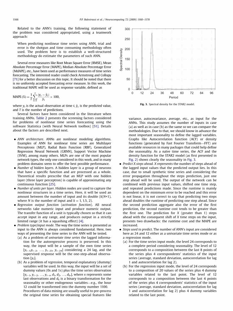
variance, autocovariance, average, etc., as input for theANNs. This study assumes the number of inputs in case(a) as well as in case (b) as the same so we can compare themethodologies. Due to that, we should know in advance themost important seasonality to define the lagged variables.Graphs like Autocorrelation function (ACF) or densityfunctions (generated by Fast Fourier Transform—FFT) areavailable resources in many packages that could help definethe seasonality. As a naıve time series, the ACF and thedensity function for the STAR2 model (as first presented inFig. 2) shows clearly the seasonality in Fig. 3.

�

Predict X steps ahead. X represents the number of steps ahead ofthe lagged input values that the predicted output lies. In thiscase, due to small synthetic time series and considering theerror propagation throughout the steps prediction, just onestep ahead will be used. The output of the network can becombined with previous input values, shifted one time step,and repeated predictions made. Since the runtime is mainlydependent on the minimum error to be reached and this erroris not linear, it is not correct to say that predicting two stepsahead doubles the runtime of predicting one step ahead. Sincethe second prediction aggregate also the error of the firstprediction, the second runtime cost tends to be greater thanthe first one. The prediction for X (greater than 1) stepsahead with the consequent shift of X time steps on the input,presents two drawbacks: the runtime cost and the MAPE areincreased. � Steps used to predict. The number of ANN’s input are considered

here as 24 and 12 either as a univariate time series mode or asa regression mode.(a) For the time series input mode, the level 24 corresponds to

a complete period considering seasonality. The level of 12corresponds to a composition between the last 8 points ofthe series plus 4 correspondents’ statistics of the inputseries (average, standard deviation, autocorrelation for lag1 and autocorrelation for lag 2).

(b) For the regression input mode, the level of 24 correspondsto a composition of 20 values of the series plus 4 dummyvariables related to the last point. The level of 12corresponds to a composition between the last 4 pointsof the series plus 4 correspondents’ statistics of the inputseries (average, standard deviation, autocorrelation for lag1 and autocorrelation for lag 2) plus 4 dummy variablesrelated to the last point.

ARTICLE IN PRESS

P.P. Balestrassi et al. / Neurocomputing 72 (2009) 1160–1178 1167

�

Phase 1 training algorithm. This factor is related to the trainingalgorithm for the MLP in a first stage and assumes three levels.(a) Backpropagation. A simple algorithm with a large number

of tuning parameters, often slow terminal convergence, butgood initial convergence.

(b) Quick propagation. An older algorithm with comparableperformance to Backpropagation in most circumstances,although it seems to perform noticeably better on someproblems.

(c) Delta-bar-delta. Another variation on Backpropagation,which occasionally seems to have better performance.

�

Phase 2 training algorithm. This factor is related to the trainingalgorithm for the MLP in a second stage and assumes threelevels.(a) Conjugate gradient descent. A good generic algorithm with

generally fast convergence.(b) Quasi-Newton. A powerful second-order training algorithm

with very fast convergence but high memory requirements.(c) Levenberg–Marquardt. An extremely fast algorithm in the

right circumstances (i.e., low-noise regression problemswith the standard sum-squared error function).

�

Epochs. An epoch is the presentation of the entire training set tothe neural network in a given phase. Increasing this number willlikely improve the accuracy of the model, but at the cost of time,and decreasing this number will likely decrease the accuracy, buttake less time. Directly related to the time series sample size thisvalue will be adopted here at the levels of 100 and 400. � Learning rate. A value between 0 and 1 that represents a tuning

variable for the training algorithms of Backpropagation, Quickpropagation and Delta-bar-delta. Lower learning rates requiremore training iterations. A higher learning rate allows the networkto converge more rapidly, however the chances of a non-optimalsolution are greater. The levels chosen here were 0.0 and 0.1.

� Initialization method. This factor defines how the weights

should be initialized at the beginning of training and assumestwo levels:(a) Random uniform. The weights are initialized to a uniformly

distributed random value, within a range whose minimumand maximum values are given. In this case, minimum andmaximum are 0 and 1.

(b) Random Gaussian. The weights are initialized to a normallydistributed random value, within a range whose mean andstandard deviation are given. In this case, N(0,1) wasadopted.

�

Stopping conditions (Target error). If the error on the training orselection test drops below the given target values, the networkis considered to have trained sufficiently well, and training isterminated. The error never drops to zero or below, so thedefault value of zero is equivalent to not having a target error. � Minimum improvement in error for training/selection. This factor

represents the minimum improvement (drop) in error thatmust be made; if the rate of improvement drops below thislevel, training is terminated. The default value of zero impliesthat training will be terminated if the error deteriorates. Onecan also specify a negative improvement rate, which isequivalent to giving a maximum rate of deterioration that willbe tolerated. The improvement is measured across a number ofepochs, called the ‘‘window’’ (see below).

� Minimum improvement in error for number of epochs. Specifies

the number of epochs across which improvement is measured.Some algorithms, including Backpropagation, demonstratenoise on the training and selection errors, and all thealgorithms may show noise in the selection error. It is thereforenot usually a good idea to halt training on the basis of a failureto achieve the desired improvement in error rate over a singleepoch. The window specifies a number of epochs over which

the error rates are monitored for improvement. Training is onlyhalted if the error fails to improve for that many epochs. If thewindow is zero, the minimum improvement threshold is notused at all. The variable levels of 1, 25 and 50 define thewindow size in determining minimum improvement. Theadopted values were considered taking into account the timeseries seasonality.

� Prune units with small fan-out weights. A neuron with small

magnitude fan-out weights (i.e., weights leading to the nextlevel) makes little contribution to the activations of the nextlayer and can be pruned, leading to a compact, faster networkwith equivalent performance. This option is particularly usefulin conjunction with Weigend weight decay that encouragesthe development of small weights precisely so that they can bepruned. Hidden units with small fan-out weights should bepruned. If a unit’s fan-out weights have smaller magnitudethan a threshold, it is a candidate for pruning.

� Prune input.

(a) y with small fan-out weights. Each input has one or moreassociated input layer neurons (more than one for somenominal inputs, and for time series networks), and the fanout on all these input neurons must be less than thethreshold for the input to be pruned.

(b) y with low sensitivity after training. A sensitivity analysis isrun after the network is trained, and input with trainingand selection sensitivity ratios below a threshold value arepruned. An input with a sensitivity pruning ratio thresholdof 1.0 makes no contribution to the network’s decision, andcan be pruned without any detriment. An input withsensitivity below 1.0 actually damages network perfor-mance, and should definitely be pruned (perhaps surpris-ingly, inputs with sensitivity below 1.0 on the selectiondata are not an uncommon occurrence, a by-product ofover-learning).

�

Weigend weight decay regularization—Phase 1. Weight decaycan be applied separately to the two phases of a two-phasealgorithm. In the phase 1 the algorithms of Backpropagation,Quick propagation, Delta-bar-delta were considered. Thisoption encourages the development of smaller weights, whichtends to reduce the problem of over-fitting, thereby potentiallyimproving generalization performance of the network, and alsoallowing you to prune the network. Weight decay works bymodifying the network’s error function to penalize largeweights—the result is an error function that compromisesbetween performance and weight size. Consequently, too largea weight decay term may damage network performanceunacceptably, and experimentation is generally needed todetermine an appropriate weight decay factor for a particularproblem domain. A study of decay factors and weight pruningshows that the number of inputs and units pruned isapproximately proportional to the logarithm of the decayfactor, and this should be borne in mind when altering thedecay factor. For example, if you use a decay factor of 0.001 andthis has insufficient effect on the weights, you might try 0.01next, rather than 0.002; conversely, if the weights were over-adjusted resulting in too much pruning, try 0.0001. There isalso a secondary factor in weight decay, which is usually left atthe default value of 1.0. � Weigend weight decay regularization—Phase 2. In this phase, the

algorithms of Conjugate gradient descent, Quasi-Newton, andLevenberg–Marquardt were considered.

� Backpropagation tuning:

(a) Adjust learning rate and momentum each epoch. UsuallyBackpropagation uses a fixed learning rate and momentumthroughout training. Some authors, however, recommendaltering these rates on each epoch (specifically, by reducing

ARTICLE IN PRESS

P.P. Balestrassi et al. / Neurocomputing 72 (2009) 1160–11781168

the learning rate—this is often counter-balanced byincreasing momentum). A higher learning rate mayconverge more quickly, but may also exhibit greaterinstability. Values of 0.1 or lower are reasonably conserva-tive—higher rates are tolerable on some problems, but noton all (especially on regression problems, where a higherrate may actually cause catastrophic divergence of theweights). Momentum is used to compensate for slowconvergence if weight adjustments are consistently in onedirection—the adjustment ‘‘picks up speed’’. Momentumusually increases the speed of convergence of Backpropa-gation considerably, and a higher rate can allow you todecrease the learning rate to increase stability withoutsacrificing much in the way of convergence speed.

(b) Shuffle presentation order of cases each epoch. In this case,the Backpropagation algorithm adjusts the weights of thenetwork as each training case is presented (rather than thebatch approach, which calculates an average adjustmentacross all training cases, and applies a single adjustment atthe end of the epoch). If the shuffle option is checked, theorder of presentation is adjusted each epoch. This makesthe algorithm somewhat less prone to stick in localminima, and partially accounts for Backpropagation’sgreater robustness than the more advanced second-ordertraining algorithms in this respect.

(c) Add Gaussian noise. Gaussian noise of the given deviation isadded to the target output value on each case. This isanother regularization technique, which can reduce thetendency of the network to overfit. The best level of noiseis problem dependent, and must be determined byexperimentation. The standard deviation of the Gaussiannoise added to the target output during training in thiscase is 0.10.

�

Quick propagation tuning:(a) Learning rate. Specify the initial learning rate, applied in the

first epoch; subsequently, the quick propagation algorithmdetermines weight changes independently for each weight.

(b) Acceleration. Specify the maximum rate of geometricincrease in the weight change, which is permitted. Forexample, an acceleration of two will permit the weightchange to no more than double on each epoch. Thisprevents numerical difficulties otherwise caused by non-concave error surfaces.

(c) Add Gaussian noise. Same as for Backpropagation.

� Delta-bar-delta tuning:

(a) Learning rate. Specify the initial learning rate used for allweights on the first epoch. Subsequently, each weightdevelops its own learning rate. Specify the linear incre-ment added to a weight’s learning rate if the slope remainsin a consistent direction. Specify the geometric decayfactor used to reduce a weight’s learning rate if the slopechanges direction. Specify the smoothing coefficient usedto update the bar-Delta smoothed gradient. It must lie inthe range (0,1). If the smoothing factor is high, the bar-Delta value is updated only slowly to take into accountchanges in gradient. On a noisy error surface this allowsthe algorithm to maintain a high learning rate consistentwith the underlying gradient; however, it may also lead toovershoot of minima, especially on an already-smootherror surface.

(b) Add Gaussian noise. Same as for Backpropagation.

� Sample size. The set of time series will be represented having an

hourly based seasonality corresponding to 1 week (168 points),2 weeks and 4 weeks (that is approximately a month). This is atentative to resemble practical problems. The seed for therandom error was recorded for future benchmarking purposes.

�

Sampling method:(a) Random resampling. In the random (Monte Carlo) resam-

pling method the subsets are randomly sampled from theavailable cases. Each available case is assigned to one of thethree subsets (training, selection or test) using theproportion 2:1:1.

(b) Cross-validated resampling. The cross validation is N-fold,where N is the number of samples taken. The available datais divided into N parts, and one part is assigned to the testset on each sample. The remainder is divided among thetraining and selection subsets, and you can specify howmany are put in each. Many authors, when using crossvalidation, do not use a selection set at all, on the basis thatany bias contributed by a particular network can becompensated for by averaging predictions across thenetworks in an ensemble. However, it is probably stilladvisable to take some steps to alleviate over-learning,which might include use of a selection set, weight decay, orstopping conditions determined experimentally to bereasonable for the problem domain.

3.3. Designs and results

In this section, the guidelines related to the choice ofexperimental design and its statistical results will be discussed.

Considering the 24 factors in Table 2 it is interesting toevaluate the complexity of running the entire combinatorialpossibilities while simulating the ANNs. In a case where only twolevels for each factor are considered to run the completesimulation (varying one factor at a time), the number of runswould be 224. Taking into account 10 min as a rough time for eachsimulation in a fast computer, the time required would be relatedto centuries for all the combinations. It is unlikely that trial anderror, the most used method, find the best combination for theANN’s training. Fortunately, a great number of designs areavailable nowadays to deal with screening procedures.

Some potential designs and strategies are suitable for the firstscreening phase where the goals are to identify those factors thatmay affect the performance the most, screen out the irrelevantvariables and establish the cause and effect relationships. Thescreening method used depends on the number of factors thatneed to be screened. Fractional factorial designs are amongst themost widely used types of design in industry (Myers andMontgomery [72]). However, those are not practical when thenumber of factors exceeds 20 and there are more than two levels.Other screening methods for large numbers of variables include(i) Group Screening Design (Kleijnen [73]) with some drawbackrelated to group formation; (ii) Sequential Bifurcation (Trocineand Malone [74]), with a drawback of being limited to quantitativevariables; (iii) the Iterated Fractional Designs (Andres and Hajas[75]) with a drawback of not being able to evaluate interaction,and (iv) the Trocine Screening Procedure (Trocine [76]) with adrawback of only being able to evaluate three to four criticalfactors. In general, these methods are useful and much better thanthe traditional trial and error strategy.

3.3.1. Design 1: Taguchi screening design for 19 factors

In this work, a Taguchi approach was considered as screeningdesign due to the factor’s structure presented in Table 2, with 11two-level factors, 8 three-level factors and 3 conditional four-levelfactors. Out of 24 factors, 2 of them (ANN architecture and Predict

X steps ahead) were established as a constraint and excluded fromthe design due to the following reasons: (i) The ANN architecturehas to be defined a priori so the factors could be the same. Using a

ARTICLE IN PRESS

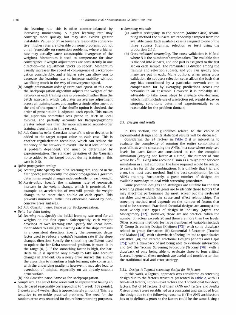
Table 3Taguchi crossed array

Inner Array (L36) Outer Array (L4)

11 two-level factors 8 three-level factors y1 y2 y3 y4

BP 1 1 2 2

QP 1 2 1 2

DD 1 2 2 1

HL OF PT SP Ep LR IM SC ET PU SM UL P1 P2 EE PI W1 W2 SS MAPE

1 1 1 1 1 1 1 1 1 1 1 1 1 1 1 1 1 1 1 1 0.056 0.066 0.071 0.073

2 1 1 1 1 1 1 1 1 1 1 1 2 2 2 2 2 2 2 2 0.073 0.078 0.073 0.075

3 1 1 1 1 1 1 1 1 1 1 1 3 3 3 3 3 3 3 3 0.084 0.076 0.074 0.085

4 1 1 1 1 1 2 2 2 2 2 2 1 1 1 1 2 2 2 2 0.093 0.100 0.102 0.096

5 1 1 1 1 1 2 2 2 2 2 2 2 2 2 2 3 3 3 3 0.092 0.096 0.091 0.097

6 1 1 1 1 1 2 2 2 2 2 2 3 3 3 3 1 1 1 1 0.103 0.095 0.103 0.102

7 1 1 2 2 2 1 1 1 2 2 2 1 1 2 3 1 2 3 3 0.093 0.085 0.095 0.094

8 1 1 2 2 2 1 1 1 2 2 2 2 2 3 1 2 3 1 1 0.088 0.098 0.103 0.101

9 1 1 2 2 2 1 1 1 2 2 2 3 3 1 2 3 1 2 2 0.150 0.147 0.144 0.142

10 1 2 1 2 2 1 2 2 1 1 2 1 1 3 2 1 3 2 3 0.041 0.039 0.046 0.044

11 1 2 1 2 2 1 2 2 1 1 2 2 2 1 3 2 1 3 1 0.090 0.093 0.091 0.097

12 1 2 1 2 2 1 2 2 1 1 2 3 3 2 1 3 2 1 2 0.091 0.093 0.092 0.097

13 1 2 2 1 2 2 1 2 1 2 1 1 2 3 1 3 2 1 3 0.075 0.071 0.063 0.067

14 1 2 2 1 2 2 1 2 1 2 1 2 3 1 2 1 3 2 1 0.131 0.123 0.121 0.123

15 1 2 2 1 2 2 1 2 1 2 1 3 1 2 3 2 1 3 2 0.084 0.093 0.098 0.086

16 1 2 2 2 1 2 2 1 2 1 1 1 2 3 2 1 1 3 2 0.107 0.095 0.097 0.093

17 1 2 2 2 1 2 2 1 2 1 1 2 3 1 3 2 2 1 3 0.132 0.124 0.128 0.129

18 1 2 2 2 1 2 2 1 2 1 1 3 1 2 1 3 3 2 1 0.117 0.105 0.103 0.107

19 2 1 2 2 1 1 2 2 1 2 1 1 2 1 3 3 3 1 2 0.124 0.131 0.137 0.125

20 2 1 2 2 1 1 2 2 1 2 1 2 3 2 1 1 1 2 3 0.114 0.120 0.116 0.115

21 2 1 2 2 1 1 2 2 1 2 1 3 1 3 2 2 2 3 1 0.094 0.099 0.100 0.100

22 2 1 2 1 2 2 2 1 1 1 2 1 2 2 3 3 1 2 1 0.103 0.106 0.112 0.119

23 2 1 2 1 2 2 2 1 1 1 2 2 3 3 1 1 2 3 2 0.108 0.117 0.116 0.117

24 2 1 2 1 2 2 2 1 1 1 2 3 1 1 2 2 3 1 3 0.115 0.107 0.105 0.110

25 2 1 1 2 2 2 1 2 2 1 1 1 3 2 1 2 3 3 1 0.109 0.117 0.113 0.111

26 2 1 1 2 2 2 1 2 2 1 1 2 1 3 2 3 1 1 2 0.063 0.065 0.066 0.062

27 2 1 1 2 2 2 1 2 2 1 1 3 2 1 3 1 2 2 3 0.111 0.111 0.115 0.115

28 2 2 2 1 1 1 1 2 2 1 2 1 3 2 2 2 1 1 3 0.102 0.111 0.113 0.118

29 2 2 2 1 1 1 1 2 2 1 2 2 1 3 3 3 2 2 1 0.088 0.081 0.091 0.078

30 2 2 2 1 1 1 1 2 2 1 2 3 2 1 1 1 3 3 2 0.149 0.136 0.135 0.129

31 2 2 1 2 1 2 1 1 1 2 2 1 3 3 3 2 3 2 2 0.096 0.103 0.104 0.105

32 2 2 1 2 1 2 1 1 1 2 2 2 1 1 1 3 1 3 3 0.087 0.088 0.076 0.085

33 2 2 1 2 1 2 1 1 1 2 2 3 2 2 2 1 2 1 1 0.098 0.099 0.105 0.099

34 2 2 1 1 2 1 2 1 2 2 1 1 3 1 2 3 2 3 1 0.099 0.107 0.107 0.090

35 2 2 1 1 2 1 2 1 2 2 1 2 1 2 3 1 3 1 2 0.063 0.056 0.062 0.067

36 2 2 1 1 2 1 2 1 2 2 1 3 2 3 1 2 1 2 3 0.067 0.070 0.055 0.064

P.P. Balestrassi et al. / Neurocomputing 72 (2009) 1160–1178 1169

different ANN would imply in different factors and levels thatdoes not make sense in this case. For instance, only MLP was hereevaluated. (ii) The prediction horizon was defined for a single stepahead, which simplifies dramatically the comparison results. Justincreasing this interval does not add any major contribution to theANN optimization and to the research objective.

The Taguchi design with its structure of inner/outer arrayallows a good fitting for the factors in Table 2 as presented inTable 3. In this screening phase, the two and three-level factorsare used as inner array in a L36 Taguchi design. The conditionalfactors (BP, QP and DD) are related to the tuning of the factor P1(Phase 1 training algorithm) for the MLP and will be used here asouter array structure. This means that when a level (Back-

propagation, Quick Propagation or Delta-bar-Delta) for the factorP1 is chosen, a specific tuning will be used for each level. A L4

Taguchi design for the tuning y1yy4 was then chosen. This designis based on the levels (A, B and C of the tuning parameters of thefactors BP, QP and DD according to Table 2. The response variable isthe metric MAPE and the outer array structure is conditionalto the above-mentioned level of the factor P1. When P1 assume,for example, level 1 (that means Backpropagation) the tuning willsetup A (Adjust learning rate and momentum each epoch), B (Shuffle

presentation order of cases each epoch) and C (Add Gaussian noise)as Yes (1) or No (2) according to the L4 Taguchi design. Each run of

L36 will be repeated 4 times through y1 to y4. The idea here was touse a design with minimal number of runs. In this case the L4

Taguchi design (with 4 runs) is similar to a 23�1 classical design(with also 4 runs). Both designs can be considered as of resolutionIII, were the alias structure is similar. For a high order design,like the full factorial design, the number of runs would bedoubled (and so the number of simulations). In this case, in spiteof the gain of resolution of a higher order design, the runtime cost isdecisive. Since the L4 Taguchi design is used only on the screeningphase, and only for conditional factors, the confounding effects(due to the DOE resolution) could be solved in the next designs.The following experimental design was obtained and the MAPE,considering 24 or 12 points out of training sample, was thencalculated.

Taguchi recommends that the mean response for each run inthe inner array and also the signal-to-noise ratio (SN) need to beevaluated. The SN here can be computed using the followingstandard smaller-the-better function:

SN ¼ �10 log1

n

Xn

i¼1

y2i

!with n ¼ 4.

The SN is expressed on a decibel scale and at this screeninglevel, the Taguchi strategy of analysis is just to pick the winner. The

ARTICLE IN PRESS

P.P. Balestrassi et al. / Neurocomputing 72 (2009) 1160–11781170

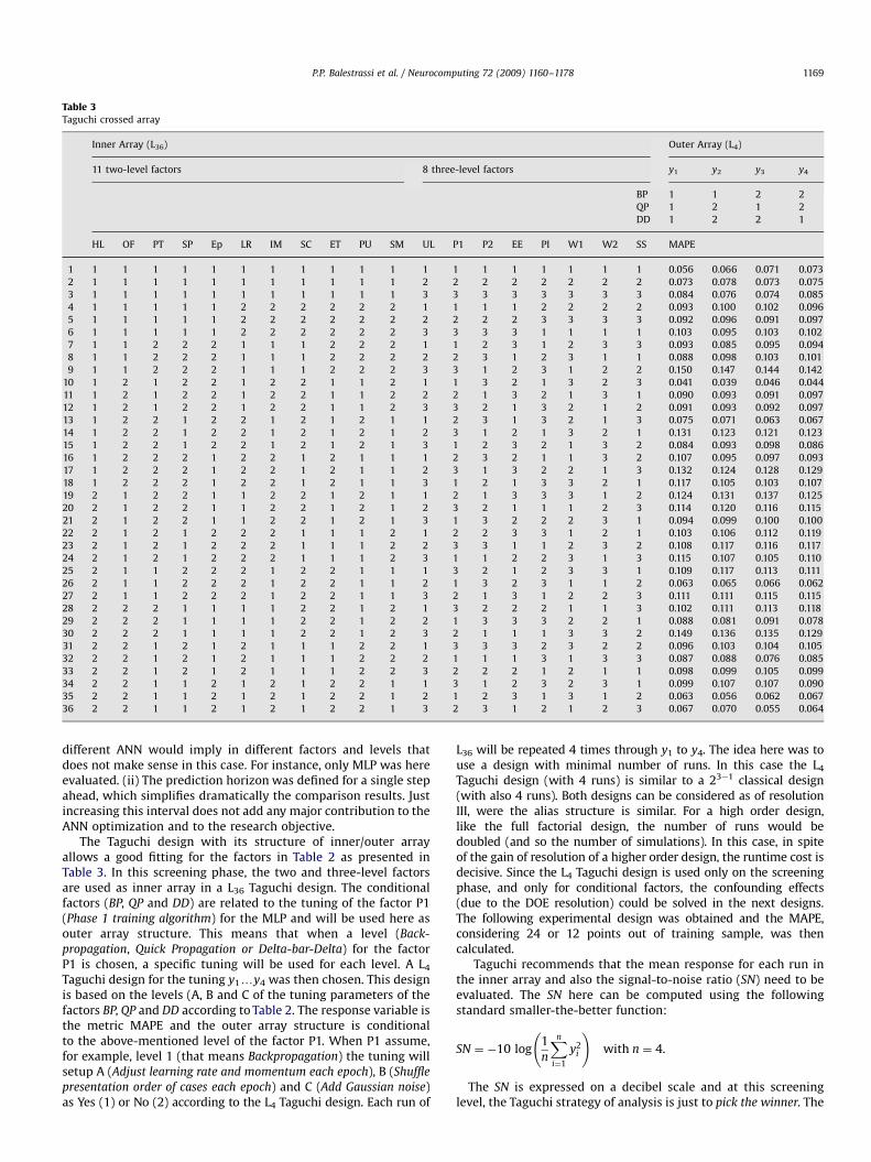
best level values for computed SNs are always the greatest. Valuesfor the mean depend on the problem type and here MAPE isdesirable as smaller as possible. Taguchi advocates claim that theuse of SN ratio generally eliminates the need for examiningspecific interactions between the inner array and the outer arrayfactors. By observing both the mean and the SN ratio, as shown inFig. 4, it is easy to pick the factors level that result at the sametime in smaller values of mean and greater values of SNs.Borderline values will be left for future designs where interactionscould be better evaluated.

From this screening analysis, some results were established,considering the MAPE mean and the SN ratio:

(a)

The factors IM, SC, PU, EE and PI were considered notsignificant and further designs could either eliminate ordefine them as a noise factors. These are the factors whicheffects were constant for the factor’s level.

(b)

The factors PT, P1 and P2 were considered significant and theirlevels were established for future designs. These are thefactors which effects have resulted in both greater SN andsmaller mean, that means P1 (level 1 ¼ Backpropagation), P2(level 3 ¼ Levenberg– Marquardt) and PT (level 1 ¼ Univariate

time series).

(c) The factors HL, SM, UL, W1, W2, SS, OF, SP, Ep, LR and ET were

considered borderlines because it was not so clear toeliminate or to select the factor’s level. Here, furtherinvestigation is needed.

(d)

Due to clear similarities in terms of SN as well as in terms ofmean, the three-level borderline factors (UL, W1, W2 and SS)were then defined as two-level factors.

21

22

21

20

21 21 21 21

21

22

21

20

21 21 21 21

21

22

21

20

321 321 321

321

22

21

20

321 321 321

HL

Mea

n of

SN

ratio

s

OF PT SP Ep

LR IM SC ET PU

SM UL P1 P2 EE

PI W1 W2 SS

Main Effects Plot for SN ratios

Signal-to-noise: Smaller is better

1.0 1.5 4.0

Fig. 4. Mean and SN for the Tag

(e)

Mea

n of

Mea

ns

uchi

For the noise variables, statistical t-tests have not rejected thenull hypothesis of equal means. In this way the authors werequite comfortable in neglecting the noise variables in furtherdesigns.

(f)

One interesting finding is related to the number of inputspruned and the input mode. For the 24 points for a problem ofunivariate time series, the number of inputs pruned is smallfor most cases (the average was 3). This means that all thepoints are important to establish the prediction. As a problemof regression, were pre-processing was imposed to the timeseries input, the pruned number was statistically greater thanfor the univariate time series mode (the average numberwas 7). This means that some pre-processing techniques havenot added any contribution for the neural network efficiency.

3.3.2. Design 2: 21127III fractional factorial design for 11 factors

For the 11 two-level remaining factors a resolution IIIPlackett–Burman fractional factorial design or a L12 Taguchidesign could be used with potentially same results and usingthe minimum amount of 12 runs. Some close options could be theL16 Taguchi design or the resolution III Fractional Factorial21127

III design, both with 16 runs. Using both Plackett–Burmanand Taguchi designs, the interaction analysis is often difficult tointerpret in practice. If the choice is between a geometric 21127

III

design with 16 runs or a 12-run Plackett–Burman design that mayhave to be folded over (thereby requiring 24 runs) the geometricdesign may turn out to be a better choice (Montgomery, 1993).The geometric fractional factorial 21127

III design (in coded units)was then used here and the experimental results are shown in

21

0.11

0.10

0.09

21 21 21 21

21

0.11

0.10

0.09

21 21 21 21

21

0.11

0.10

0.09

4.01.51.0 321 321 321

321

0.11

0.10

0.09

321 321 321

HL OF PT SP Ep

LR IM SC ET PU

SM UL P1 P2 EE

PI W1 W2 SS

Main Effects Plot for Means

design (STAR2 model).

ARTICLE IN PRESS

P.P. Balestrassi et al. / Neurocomputing 72 (2009) 1160–1178 1171

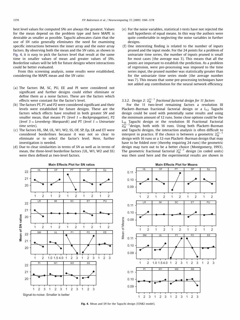
Table 4. MAPE 1, MAPE 2 and MAPE 3 consider the noise variablesat their lowest, middle and upper levels, respectively.

Fig. 5 presents the Pareto chart and the main effects plot forthe factors in Table 4.

For this second screening analysis, the results were:

(a)

Tabl

211�III

1

2

3

4

5

6

7

8

9

10

11

12

13

14

15

16

The factors ET and W1 were considered not significant andfurther designs could either eliminate or define them as anoise factor. These are factors which effects were constant forthe factor’s level.

ET

HL.SM

HL.LR

W1

HL.Ep

HL.UL

OF

SS

UL

Ep

HL

SM

W2

SP

LR

0.040.030.020.010.00

Term

Effect

0.03279

Pareto Chart of the Effects(response is MAPE, Alpha = 0.05)

Lenth's PSE =0.0127575

Fig. 5. 211�7III Design

e 47 Design

HL SM UL W1 W2 SS OF SP

�1 �1 �1 �1 �1 �1 �1 �1

1 �1 �1 �1 1 �1 1 1

�1 1 �1 �1 1 1 �1 1

1 1 �1 �1 �1 1 1 �1

�1 �1 1 �1 1 1 1 �1

1 �1 1 �1 �1 1 �1 1

�1 1 1 �1 �1 �1 1 1

1 1 1 �1 1 �1 �1 �1

�1 �1 �1 1 �1 1 1 1

1 �1 �1 1 1 1 �1 �1

�1 1 �1 1 1 �1 1 �1

1 1 �1 1 �1 �1 �1 1

�1 �1 1 1 1 �1 �1 1

1 �1 1 1 �1 �1 1 �1

�1 1 1 1 �1 1 �1 �1

1 1 1 1 1 1 1 1

(b)

Mea

n

(STA

Ep

1

�1

�1

1

�1

1

1

�1

�1

1

1

�1

1

�1

�1

1

The factor LR was considered significant and its level could beestablished for future designs. This is a factor which effect hasresulted in smaller error mean.

(c)

The factors HL, SM, UL, W2, SS, OF, SP, and Ep were con-sidered borderlines because it was not so clear to eliminate orto select the factor’s level. Here, further investigation isneeded.

(d)

For the noise variables, statistical t-tests have not rejected thenull hypothesis of equal means. As in design 1 the authorswere quite comfortable in neglecting the tuning variables in

1-1

0.100

0.075

0.0501-1 1-1 1-1

1-1

0.100

0.075

0.0501-1 1-1 1-1

1-1

0.100

0.075

0.0501-1 1-1

HL OF SP Ep

LR ET SM UL

W1 W2 SS

Main Effects Plot for MAPE

R2 model).

LR ET MAPE 1 MAPE 2 MAPE 3 Mean

1 1 0.060 0.073 0.068 0.067

�1 �1 0.060 0.054 0.054 0.056

�1 1 0.012 0.004 0.003 0.006

1 �1 0.099 0.097 0.092 0.096

1 �1 0.072 0.074 0.074 0.074

�1 1 0.109 0.093 0.096 0.099

�1 �1 0.110 0.099 0.093 0.101

1 1 0.056 0.055 0.053 0.055

1 1 0.105 0.113 0.106 0.108

�1 �1 0.041 0.038 0.046 0.042

�1 1 0.027 0.025 0.024 0.025

1 �1 0.105 0.112 0.114 0.110

1 �1 0.083 0.080 0.080 0.081

�1 1 0.118 0.118 0.121 0.119

�1 �1 0.080 0.097 0.087 0.088

1 1 0.093 0.095 0.105 0.098

ARTICLE IN PRESS

Tabl

2824IV

1

2

3

4

5

6

7

8

9

10

11

12

13

14

15

16

P.P. Balestrassi et al. / Neurocomputing 72 (2009) 1160–11781172

further designs. This mean that the setup obtained onprevious setup, using Taguchi design, was coherent.

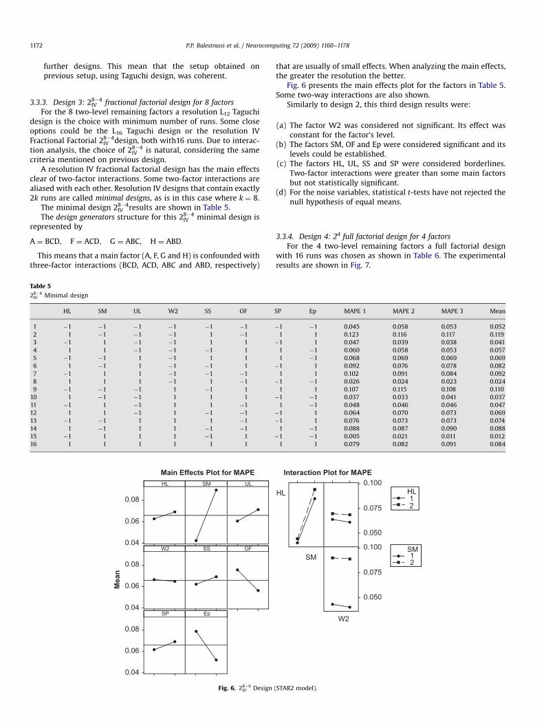
3.3.3. Design 3: 2824IV fractional factorial design for 8 factors

For the 8 two-level remaining factors a resolution L12 Taguchidesign is the choice with minimum number of runs. Some closeoptions could be the L16 Taguchi design or the resolution IVFractional Factorial 2824

IV design, both with16 runs. Due to interac-tion analysis, the choice of 2824

IV is natural, considering the samecriteria mentioned on previous design.

A resolution IV fractional factorial design has the main effectsclear of two-factor interactions. Some two-factor interactions arealiased with each other. Resolution IV designs that contain exactly2k runs are called minimal designs, as is in this case where k ¼ 8.

The minimal design 2824IV results are shown in Table 5.

The design generators structure for this 2824IV minimal design is

represented by

A ¼ BCD; F ¼ ACD; G ¼ ABC; H ¼ ABD:

This means that a main factor (A, F, G and H) is confounded withthree-factor interactions (BCD, ACD, ABC and ABD, respectively)

e 5

Minimal design

HL SM UL W2 SS OF

�1 �1 �1 �1 �1 �1

1 �1 �1 �1 1 �1

�1 1 �1 �1 1 1

1 1 �1 �1 �1 1

�1 �1 1 �1 1 1

1 �1 1 �1 �1 1

�1 1 1 �1 �1 �1

1 1 1 �1 1 �1

�1 �1 �1 1 �1 1

1 �1 �1 1 1 1

�1 1 �1 1 1 �1

1 1 �1 1 �1 �1

�1 �1 1 1 1 �1

1 �1 1 1 �1 �1

�1 1 1 1 �1 1

1 1 1 1 1 1

0.08

0.06

0.04

0.08

0.06

0.04

0.08

0.06

0.04

HL

Mean

SM UL

W2 SS OF

SP Ep

Main Effects Plot for MAPE

Fig. 6. 28�4IV Design

that are usually of small effects. When analyzing the main effects,the greater the resolution the better.

Fig. 6 presents the main effects plot for the factors in Table 5.Some two-way interactions are also shown.

Similarly to design 2, this third design results were:

(a)

SP

�1

1

�1

1

1

�1

1

�1

1

�1

1

�1

�1

1

�1

1

HL

In

(STAR

The factor W2 was considered not significant. Its effect wasconstant for the factor’s level.

(b)

The factors SM, OF and Ep were considered significant and itslevels could be established.

(c)

The factors HL, UL, SS and SP were considered borderlines.Two-factor interactions were greater than some main factorsbut not statistically significant.

(d)

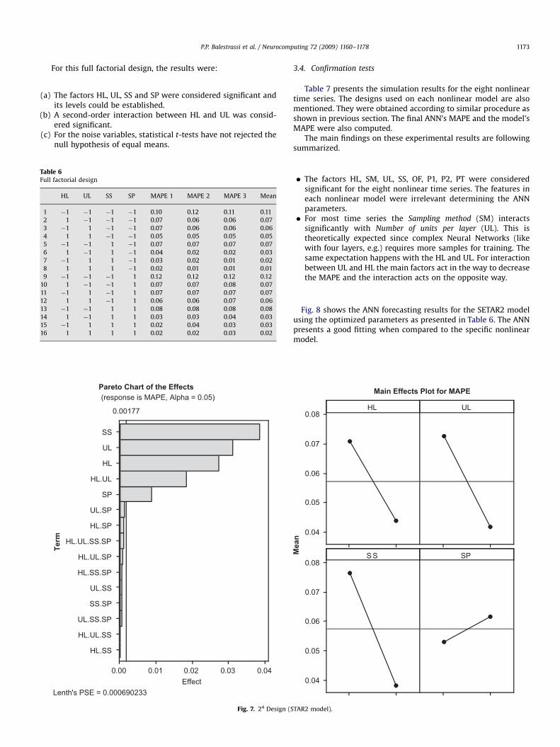
For the noise variables, statistical t-tests have not rejected thenull hypothesis of equal means.

3.3.4. Design 4: 24 full factorial design for 4 factors

For the 4 two-level remaining factors a full factorial designwith 16 runs was chosen as shown in Table 6. The experimentalresults are shown in Fig. 7.

Ep MAPE 1 MAPE 2 MAPE 3 Mean

�1 0.045 0.058 0.053 0.052

1 0.123 0.116 0.117 0.119

1 0.047 0.039 0.038 0.041

�1 0.060 0.058 0.053 0.057

�1 0.068 0.069 0.069 0.069

1 0.092 0.076 0.078 0.082

1 0.102 0.091 0.084 0.092

�1 0.026 0.024 0.023 0.024

1 0.107 0.115 0.108 0.110

�1 0.037 0.033 0.041 0.037

�1 0.048 0.046 0.046 0.047

1 0.064 0.070 0.073 0.069

1 0.076 0.073 0.073 0.074

�1 0.088 0.087 0.090 0.088

�1 0.005 0.021 0.011 0.012

1 0.079 0.082 0.091 0.084

0.100

0.075

0.050

0.100

0.075

0.050

SM

W2

12

HL

12

SM

teraction Plot for MAPE

2 model).

ARTICLE IN PRESS

P.P. Balestrassi et al. / Neurocomputing 72 (2009) 1160–1178 1173

For this full factorial design, the results were:

(a)

TablFull

1

2

3

4

5

6

7

8

9

10

11

12

13

14

15

16

The factors HL, UL, SS and SP were considered significant andits levels could be established.

(b)

A second-order interaction between HL and UL was consid-ered significant.

(c)

For the noise variables, statistical t-tests have not rejected thenull hypothesis of equal means.

e 6factorial design

HL UL SS SP MAPE 1 MAPE 2 MAPE 3 Mean

�1 �1 �1 �1 0.10 0.12 0.11 0.11

1 �1 �1 �1 0.07 0.06 0.06 0.07

�1 1 �1 �1 0.07 0.06 0.06 0.06

1 1 �1 �1 0.05 0.05 0.05 0.05

�1 �1 1 �1 0.07 0.07 0.07 0.07

1 �1 1 �1 0.04 0.02 0.02 0.03

�1 1 1 �1 0.03 0.02 0.01 0.02

1 1 1 �1 0.02 0.01 0.01 0.01

�1 �1 �1 1 0.12 0.12 0.12 0.12

1 �1 �1 1 0.07 0.07 0.08 0.07

�1 1 �1 1 0.07 0.07 0.07 0.07

1 1 �1 1 0.06 0.06 0.07 0.06

�1 �1 1 1 0.08 0.08 0.08 0.08

1 �1 1 1 0.03 0.03 0.04 0.03

�1 1 1 1 0.02 0.04 0.03 0.03

1 1 1 1 0.02 0.02 0.03 0.02

HL.SS

HL.UL.SS

UL.SS.SP

SS.SP

UL.SS

HL.SS.SP

HL.UL.SP

HL.UL.SS.SP

HL.SP

UL.SP

SP

HL.UL

HL

UL

SS

0.040.030.020.010.00

Term

Effect

0.00177

Pareto Chart of the Effects

(response is MAPE, Alpha = 0.05)

Lenth's PSE = 0.000690233

Fig. 7. 24 Design (S

3.4. Confirmation tests

Table 7 presents the simulation results for the eight nonlineartime series. The designs used on each nonlinear model are alsomentioned. They were obtained according to similar procedure asshown in previous section. The final ANN’s MAPE and the model’sMAPE were also computed.

The main findings on these experimental results are followingsummarized.

�

Mean

TAR

The factors HL, SM, UL, SS, OF, P1, P2, PT were consideredsignificant for the eight nonlinear time series. The features ineach nonlinear model were irrelevant determining the ANNparameters.

� For most time series the Sampling method (SM) interacts

significantly with Number of units per layer (UL). This istheoretically expected since complex Neural Networks (likewith four layers, e.g.) requires more samples for training. Thesame expectation happens with the HL and UL. For interactionbetween UL and HL the main factors act in the way to decreasethe MAPE and the interaction acts on the opposite way.

Fig. 8 shows the ANN forecasting results for the SETAR2 modelusing the optimized parameters as presented in Table 6. The ANNpresents a good fitting when compared to the specific nonlinearmodel.

0.08

0.07

0.06

0.05

0.04

0.08

0.07

0.06

0.05

0.04

HL UL

S S SP

Main Effects Plot for MAPE

2 model).

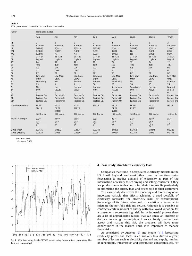
ARTICLE IN PRESS

Table 7ANN parameters chosen for the nonlinear time series

Factor Nonlinear model

SAR BL1 BL2 TAR NAR NMA STAR1 STAR2

HL 2�� 2� 2� 2� 2� 2� 2�� 2��

SM Random� Random�� Random� Random� Random� Random� Random�� Random��

UL 2(N+1)�� 2(N+1)� 2(N+1)� 2(N+1)�� 2(N+1)� 2(N+1)� 2(N+1)�� 2(N+1)��

W1 0.0001 0.0001 0.0001 0.001 0.001 No 0.001 0.001

W2 0.0001 No No 0.001 0.0001 No 0.001 0.001

SS 21�24� 21�24� 21�24� 21�24� 21�24� 21�24� 21�24�� 21�24��

OF Logistic� Logistic� Logistic� Logistic� Logistic� Logistic� Logistic� Logistic�

SP 24 12� 12 12� 24 12� 24 12�

Ep 400 400 400� 100 100 400 400� 400�

LR 0.9� 0.9 0.9 0.9� 0.9� 0.1 0.9� 0.9�

ET 0 �0.1 �0.1 0 0 �0.1 0 0

P1 BP� BP� BP� BP� BP� BP� BP� BP�

P2 Lev. Mar.� Lev. Mar.�� Lev. Mar.�� Lev. Mar.� Lev. Mar.� Lev. Mar.� Lev. Mar.� Lev. Mar.��

PT Univ.�� Univ.�� Univ.�� Univ.�� Univ.�� Univ.�� Univ.�� Univ.��

PU Sensitivity No Fan-out Fan-out Sensitivity No No Fan-out

EE 25 1 1 50 25 50 25 25

PI No No Fan-out Fan-out Sensitivity Sensitivity Fan-out Fan-out

IM U(0,1) U(0,1) U(0,1) N(0,1) N(0,1) U(0,1) N(0,1) N(0,1)

SC 0 0.1 0.1 0 0.1 0 0 0

BP Factors On Factors On Factors On Factors On Factors On Factors On Factors On Factors On

QP Factors On Factors On Factors On Factors On Factors On Factors On Factors On Factors On

DD Factors On Factors On Factors On Factors On Factors On Factors On Factors On Factors On

Main interactions HL.UL HL.UL HL.UL SM.UL HL.UL HL.UL HL.UL HL.UL

SM.UL OF.P2 SM.UL OF.P2 P2.PT SM.UL

SM.UL SM.UL

Tag L36 L4 Tag L36 L4 Tag L36 L4 Tag L36 L4 Tag L36 L4 Tag L36 L4 Tag L36 L4 Tag L36 L4

Factorial designs 211�7III 210�6

III 210�6III 29�5

III 211�7III 211�7

III 212�8III 211�7

III

27�3IV 26�2

IV 27�3IV 26�2

IV 28�4IV 27�3

IV 28�4IV 28�4

IV

23 23 24 23 24 2325�1

V24

MAPE (ANN) 0.0435 0.0292 0.0194 0.0248 0.0366 0.0468 0.0246 0.0282

MAPE (Model) 0.0623 0.061 0.0656 0.0781 0.0664 0.0789 0.075 0.0788

� P-valueo0.05.�� P-valueo0.001.

355 361 367 373 379 385 391 397 403 409 415 421 427 433

-5

-4

-3

-2

-1

0

1

2 STAR2 Model STAR2 ANN

Fig. 8. ANN forecasting for the SETAR2 model using the optimized parameters. The

data test is amplified.

P.P. Balestrassi et al. / Neurocomputing 72 (2009) 1160–11781174

4. Case study: short-term electricity load

Companies that trade in deregulated electricity markets in theUS, Brazil, England, and most other countries use time seriesforecasting to predict demand of electricity as part of theinformation necessary to set buying and selling contracts. If theyare production or trade companies, their interests lie particularlyin optimizing the energy load and prices sold to their costumers.

This case study deals with the modeling and forecasting of animportant variable that affects achieving a good portfolio ofelectricity contracts: the electricity load (or consumption).Knowledge of its future value and its variation is essential tocalculate the portfolio risk and return. Although it is possible tocontract a certain amount of energy with no allowed variation, fora consumer it represents high risk. In the industrial process thereare a lot of unpredictable factors that can cause an increase ordecrease in energy consumption. If an electricity producer canaccept and manage this risk, the producer will have moreopportunities in the market. Thus, it is important to managethese risks.

As considered by Angelus [2] and Mount [41], forecastingelectricity prices and loads is an arduous task due to a greatnumber of factors such as electricity demand and supply, numberof generations, transmission and distribution constraints, etc. For

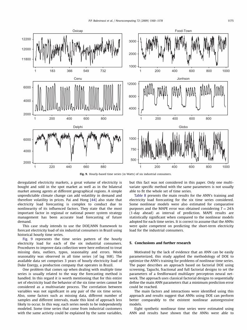
ARTICLE IN PRESS

1

12200

12000

11800

1

3000

2000

1000

1

6000

4000

2000

1

12000

8000

4000

1

6000

4000

2000

1

1000

Oxicap Food-Town

Cenu Jonhson

Delphi Globo

183 366 549 732 200 400 600 800 1000

200 400 600 800 200 400 600 800

750

500

1000800600400200880660440220

Fig. 9. Hourly-based time series (in Watts) of six industrial consumers.

P.P. Balestrassi et al. / Neurocomputing 72 (2009) 1160–1178 1175

deregulated electricity markets, a great volume of electricity isbought and sold in the spot market as well as in the bilateralmarket among agents at different geographical regions. A simpleunpredictable climate change can add volatility in demand andtherefore volatility in prices. Pai and Hong [44] also state thatelectricity load forecasting is complex to conduct due tononlinearity of its influenced factors. They state that the mostimportant factor in regional or national power system strategymanagement has been accurate load forecasting of futuredemand.

This case study intends to use the DOE/ANN framework toforecast electricity load of six industrial consumers in Brazil usinghistorical hourly time series.

Fig. 9 represents the time series pattern of the hourlyelectricity load for each of the six industrial consumers.Procedures to improve data collection were here enforced to treatmissing data, outliers, typos, seasonality and errors. Weekseasonality was observed in all time series (of lag 168). Theavailable data set comprises 3 years of hourly electricity load ofDuke Energy, a production company that operates in Brazil.

One problem that comes up when dealing with multiple timeseries is usually related to the way the forecasting method ishandled. In this regard it is worth mentioning that for this entireset of electricity load the behavior of the six time series cannot beconsidered as a multivariate process. The correlation betweenvariables was not significant in any pair of the six time series.Also, some factors such as missing data, different number ofsamples and different intervals, made this kind of approach lesslikely to occur. In this way, each series needs to be independentlymodeled. Some time series that come from industrial customerswith the same activity could be explained by the same variables,

but this fact was not considered in this paper. Only one multi-variate specific method with the same parameters is not usuallyable to fit the whole set of time series.

Table 8 presents the main results for the ANN’s training andelectricity load forecasting for the six time series considered.Some nonlinear models were also estimated for comparativepurposes and the MAPE error was obtained considering T ¼ 24 h(1-day ahead) as interval of prediction. MAPE results arestatistically significant when compared to the nonlinear modelsadopted for each time series. It is correct to assume that the ANNswere quite competent on predicting the short-term electricityload for the industrial consumers.

5. Conclusions and further research

Motivated by the lack of evidence that an ANN can be easilyparameterized, this study applied the methodology of DOE tooptimize the ANN’s training for problems of nonlinear time series.The paper describes an approach based on factorial DOE usingscreening, Taguchi, fractional and full factorial designs to set theparameters of a feedforward multilayer perceptron neural net-work. The approach uses classical factorial designs to sequentiallydefine the main ANN parameters that a minimum prediction errorcould be reached.

The main factors and interactions were identified using thisapproach and results suggest that ANNs using DOE can performbetter comparably to the existent nonlinear autoregressivemodels.

Eight synthetic nonlinear time series were estimated usingANN and results have shown that the ANNs were able to

ARTICLE IN PRESS

Table 8ANN parameters for the six industrial electricity load consumer

Factor Electricity load

Cenu Food-Town Oxicap Delphi Johnson Globo

HL 2� 2�� 2� 2�� 2�� 2��

SM Random�� Random�� Random� Random� Random� Random��

UL 50�� 50� 50� 50�� 50� 50�

W1 No 0.001 0.001 No 0.001 0.001

W2 No 0.001 0.01 No 0.0001 0.01

SS 21�24�� 21�24� 21�24�� 21�24� 21�24� 21�24��

OF Logistic�� Logistic�� Logistic�� Logistic� Logistic� Logistic��

SP 48 24� 24 48� 24 24�

Ep 500 500 400� 400 500 400

LR 0.9� 0.9 0.9 0.9� 0.9� 0.9

ET �0.1 �0.1 0 0 0 0

P1 BP�� BP� BP� BP�� BP� BP��

P2 Lev. Mar.� Lev. Mar.�� Lev. Mar.�� Lev. Mar.� Lev. Mar.� Lev. Mar.�

PT Univ.� Univ.� Univ.�� Univ.�� Univ.�� Univ.�

PU Fan-out Fan-out Fan-out Sensitivity Fan-out Fan-out

EE 1 25 25 25 50 25

PI Fan-out Sensitivity Fan-out Sensitivity Fan-out Fan-out

IM N(0,1) U(0,1) N(0,1) N(0,1) N(0,1) U(0,1)

SC 0.1 0.1 0.1 0.1 0 0

BP Factors On Factors On Factors On Factors On Factors On Factors On

QP Factors On Factors On Factors On Factors On Factors On Factors On

DD Factors On Factors On Factors On Factors On Factors On Factors On

Main interactions HL.UL SM.UL HL.UL HL.UL HL.UL HL.UL

P2.PT OF.P2 SM.UL OF.P2 OF.P2

SM.UL SM.UL SM.UL

Tag L36 L4 Tag L36 L4 Tag L36 L4 Tag L36 L4 Tag L36 L4 Tag L36 L4

Factorial designs 210�6III 211�7

III 29�5III 210�6

III 210�6III 211�7

III

27�3IV 28�4

IV 26�2IV 27�3

IV 26�2IV 27�3

IV

24 24 23 24 23 23

MAPE (ANN) 0.102 0.053 0.113 0.095 0.872 0.105

MAPE (Model) 0.186 (STAR) 0.101 (BILINEAR)) 0.173 (BILINEAR) 0.163 (STAR) 0.107 (NAR) 0.173 (BILINEAR)

� P-valueo0.05.�� P-valueo0.001.

P.P. Balestrassi et al. / Neurocomputing 72 (2009) 1160–11781176

generalize realistic autoregressive models better than the specificmodel proposed. This general nonlinear property makes ANNs apromising alternative when forecasting these models. Six indus-trial electricity load time series were explored as a case study andresults have confirmed the proposed DOE/ANN framework.

As a further research, the following points need to be betteraddressed:

�

The evolutionary approach (e.g., genetic algorithm) have beenreferred as an exception in terms of training an ANN, in whichsuch evolution levels as connection weights, network struc-ture, learning rules, etc., are optimized using an evolutionaryalgorithm. However, studies on the evolutionary approach areusually concerned with a certain level of evolution, andresearch into the simultaneous evolution of various levels isstill in its early stage [59]. � Several different methods have been proposed for building the

optimal architecture of an ANN and consider topologicalfactors such as the number of inputs, the number of hiddenlayers and the number of neurons. The pruning algorithm [47],the polynomial time algorithm [48], the canonical decomposi-tion technique [58], and the network information criterion [42]are among these methods. None of them, however, canguarantee the best ANN solution for the nonlinear time seriesforecasting problem. One interesting research is to considerthese methods also as variable in the present DOE framework.

Acknowledgments

The authors thank the Brazilian governmental agencies ofCAPES and FAPEMIG for supporting this research.

References

[1] M.J. Aitkenhead, A.J.S. McDonald, J.J. Dawson, G. Couper, R.P. Smart, M. Billett,D. Hope, S. Palmer, A novel method for training neural networks for time-series prediction in environmental systems, Ecol. Model. 162 (2003) 87–95.

[2] A. Angelus, Electricity price forecasting in deregulated markets, Electricity J. 4(2001) 32–41.

[3] S.D. Balkin, J.K. Ord, Automatic neural network modeling for univariate timeseries, Int. J. Forecast. 16 (2000) 509–515.

[4] C. Bishop, Neural Networks for Pattern Recognition, University Press, Oxford, 1995.[5] G.E.P. Box, G.M. Jenkins, Time Series Analysis: Forecasting and Control, revised

ed., Holden-Day, San Francisco, 1976.[7] S. BuHamra, N. Smaoui, M. Gabr, The Box–Jenkins analysis and neural

networks: prediction and time series modeling, Appl. Math. Model. 27 (2003)805–815.

[8] K.K. Chan, T.A. Spedding, On-line optimization of quality in a manufacturingsystem, Int. J. Prod. Res. 39 (6) (2001) 1127–1145.

[9] T. Chen, H. Chen, Universal approximation to nonlinear operators by neuralnetworks with arbitrary activation functions and its application to dynamicalsystems, IEEE Trans. Neural Netw. 6 (1995) 911–917.

[10] R. Chen, R.S. Tsay, Functional-coefficient autoregressive models, J. Am. Stat.Assoc. 88 (1993) 298–308.

[11] B. Cheng, D.M. Titterington, Neural networks: a review from a statisticalperspective, Stat. Sci. 9 (1994) 2–54.

[12] W.C. Chiang, T.L. Urban, G.W. Baldridge, A neural network approach to mutualfund net asset value forecasting, Omega, Int. J. Manage. Sci. 24 (1996) 205–215.

ARTICLE IN PRESS

P.P. Balestrassi et al. / Neurocomputing 72 (2009) 1160–1178 1177

[13] J.G. de Gooijer, On threshold moving-average models, J. Time Ser. Anal. 19(1998) 1–18.

[14] F.X. Diebold, J.A. Nason, Nonparametric exchange rate prediction, J. Int. Econ.28 (1990) 15–332.

[16] E.U. Enemuoh, A.S. El-Gizawy, Optimal neural network model for character-ization of process-induced damage in drilling carbon fiber reinforced epoxycomposites, Mach. Sci. Technol. 7 (3) (2003) 389–400.

[17] P.H. Franses, P. van Homelen, On forecasting exchange rates using neuralnetworks, Appl. Financ. Econ. 8 (1998) 689–696.

[18] M.C. Fu, Optimization for simulation: theory vs. practice, INFORMS J. Comput.14 (2002) 192–215.

[19] M. Ghiassi, H. Saidane, D.K. Zimbra, A dynamic artificial neural networkmodel for forecasting time series events, Int. J. Forecast. 21 (2005) 341–362.

[20] C.W.J. Granger, A.P. Anderson, An Introduction to Bilinear Time Series Models,Vandenhoeck & Ruprecht, Gottingen, 1978.

[21] C.W.J. Granger, T. Terasvirta, Modelling Nonlinear Economic Relationships,Oxford University Press, 1993.

[22] J.D. Hamilton, A new approach to the economic analysis of nonstationarytime series and the business cycle, Econometrica 57 (1989) 357–384.

[23] S.L. Ho, M. Xie, T.N. Goh, A comparative study of neural network andBox–Jenkins ARIMA modeling in time series prediction, Comput. Ind. Eng. 42(2002) 371–375.

[24] K. Hornik, Some new results on neural network approximation, Neural Netw.6 (1993) 1069–1072.

[25] K. Hornik, M. Stinchcombe, H. White, Multilayer feedforward networks areuniversal approximators, Neural Netw. 2 (1989) 359–366.

[26] H.B. Hwarng, Insights into neural-network forecasting of time seriescorresponding to ARMA(p; q) structures, Omega 29 (2001) 273–289.

[27] H.B. Hwarng, H.T. Ang, A simple neural network for ARMA(p; q) time series,Omega 29 (2001) 319–333.

[28] I. Kaastra, M. Boyd, Designing a neural network for forecasting financial andeconomic time series, Neurocomputing 10 (1996) 215–236.

[29] K. Kalaitzakis, G.S. Stavrakakis, E.M. Anagnostakis, Short-term load forecast-ing based on artificial neural networks parallel implementation, ElectricPower Syst. Res. 63 (2002) 185–196.

[30] D.S.K. Karunasinghe, S.Y. Liong, Chaotic time series prediction with a globalmodel: artificial neural network, J. Hydrol. 2 (2005) 1–14.

[31] J.F.C. Khaw, B.S. Lim, L.E.N. Lim, Optimal design of neural networks using theTaguchi method, Neurocomputing 7 (1995) 225–245.

[32] K.J. Kim, Financial time series forecasting using support vector machines,Neurocomputing 55 (2003) 307–319.

[33] Y.S. Kim, B.J. Yum, Robust design of multilayer feedforward neural networks:an experimental approach, Eng. Appl. Artif. Intell. 17 (2004) 249–263.

[34] J.P.C. Kleijnen, S.M. Sanchez, T.W. Lucas, T.M. Cioppa, State-of-the-art review:a user’s guide to the brave new world of designing simulation experiments,INFORMS J. Comput. 7 (3) (2005) 263–289.

[35] N. Kohzadi, M.S. Boyd, B. Kermanshahi, I. Kaastra, A comparison of artificialneural network and time series models for forecasting commodity prices,Neurocomputing 10 (1996) 169–181.

[36] H. Krager, P. Kugle, Nonlinearities in foreign exchange markets: a differentperspective, J. Int. Money Finance 12 (1993) 195–208.

[37] T.Y. Lin, C.H. Tseng, Optimum design for artificial neural networks: anexample in a bicycle derailleur system, Eng. Appl. Artif. Intell. 13 (2000) 3–14.

[38] S. Makridakis, M. Hibon, The M3-competition: results, conclusions andimplications, Int. J. Forecast. 16 (2000) 451–476.

[39] S. Makridakis, A. Andersen, R. Carbone, R. Fildes, M. Hibon, R. Lewandowski, J.Newton, E. Parzen, R. Winkler, The accuracy of extrapolation (time series)methods: results of a forecasting competition, J. Forecast. 1 (1982) 111–153.

[40] S. Makridakis, C. Chatfield, M. Hibon, M. Lawrence, T. Mills, K. Ord, L.F.Simmons, The M-2 competition: a real-time judgmentally based forecastingstudy, Int. J. Forecast. 9 (1993) 5–23.

[41] T. Mount, Market power and price volatility in restructured markets forelectricity, Decis. Support Syst. 30 (2001) 311–325.

[42] N. Murata, S. Yoshizawa, S. Amari, Network information criterion-determin-ing the number of hidden units for an artificial neural network model, IEEETrans. Neural Netw. 5 (1994) 865–872.

[43] H. Niska, T. Hiltunen, A. Karppinen, J. Ruuskanen, M. Kolehmainen, Evolvingthe neural network model for forecasting air pollution time series, Eng. Appl.Artif. Intell. 17 (2004) 159–167.

[44] P.F. Pai, W.C. Hong, Support vector machines with simulated annealingalgorithms in electricity load forecasting, Energy Convers. Manage. 46 (2005)2669–2688.

[45] M.B. Priestley, State-dependent models: a general approach to nonlinear timeseries analysis, J. Time Ser. Anal. 1 (1980) 47–71.

[46] M. Qi, G.P. Zhang, An investigation of model selection criteria for neuralnetwork time series forecasting, Eur. J. Operat. Res. 132 (2001) 666–680.

[47] R. Reed, Pruning algorithms- a survey, IEEE Trans. Neural Netw. 4 (1993)740–747.

[48] A. Roy, L.S. Kim, S. Mukhopadhyay, A polynomial time algorithm for theconstruction and training of a class of multilayer perceptrons, Neural Netw. 6(1993) 535–545.

[49] Z. Shi, Y. Tamura, T. Ozaki, Nonlinear time series modelling with the radialbasis function-based state-dependent autoregressive model, Int. J. Syst. Sci.30 (7) (1999) 717–727.

[50] J.C. Spall, Introduction to Stochastic Search and Optimization; Estimation,Simulation, and Control, Wiley, New York, 2003.

[51] StatSoft Inc., Statistica (data analysis software system), version 7.1, 2005,/www.statsoft.comS.

[52] W. Sukthomya, J. Tannock, The optimisation of neural network para-meters using Taguchi’s design of experiments approach: an application inmanufacturing process modeling, Neural Comput. Appl. 14 (2005) 337–344.

[53] W. Sukthomya, J. Tannock, The training of neural networks to modelmanufacturing processes, J. Intell. Manuf. 16 (2005) 39–51.

[54] T. Terasvirta, D. van Dijk, M.C. Medeiros, Linear models, smooth transitionautoregressions, and neural networks for forecasting macroeconomic timeseries: a re-examination, Int. J. Forecast. 21 (2005) 755–774.

[55] H. Tong, On a threshold model, in: C.H. Chen (Ed.), Pattern Recognition andSignal Processing, Sijhoff & Noordhoff, Amsterdam, 1978.

[56] R. Tsay, Analysis of Financial Time Series, second ed., Wiley-Interscience, 2005.[57] F.M. Tseng, H.C. Yu, G.H. Tzeng, Combining neural network model with

seasonal time series ARIMA model, Technol. Forecast. Soc. Change 72 (69)(2002) 71–87.

[58] Z. Wang, C.D. Massimo, M.T. Tham, A.J. Morris, A procedure for determiningthe topology of multilayer feedforward neural networks, Neural Netw. 7(1994) 291–300.

[59] X. Yao, Evolving artificial neural networks, Proc. IEEE 87 (9) (1999) 1423–1447.[60] G.P. Zhang, An investigation of neural networks for linear time-series

forecasting, Comput. Operat. Res. 28 (2001) 1183–1202.[61] G.P. Zhang, Time series forecasting using a hybrid ARIMA and neural network

model, Neurocomputing 50 (2003) 159–175.[62] G.P. Zhang, M. Qi, Neural network forecasting for seasonal and trend time

series, Eur. J. Operat. Res. 160 (2005) 501–514.[63] G.P. Zhang, B.E. Patuwo, M.Y. Hu, Forecasting with artificial neural networks:

the state-of-the-art, Int. J. Forecast. 14 (1998) 35–62.[64] G.P. Zhang, B.E. Patuwo, M.Y. Hu, A simulation study of artificial neural

networks for nonlinear time-series forecasting, Comput. Operat. Res. 28(2001) 381–396.

[65] G. Taguchi, Systems of Experimental Design, vols. 1 & 2, UNIPUB/KrausInternational Publications, New York, 1987.

[66] Y. Bodyanskiy, S. Popov, Neural network approach to forecasting ofquasiperiodic financial time series, Eur. J. Oper. Res. 175 (3) (2006)1357–1366.

[67] M.-D. Cubiles-de-la-Vega, R.P. Mejıas, A.P. Acosta, J.M. Garcıa, Intell. DataAnal. 6 (2002) 53–65.

[68] D.E. Coleman, D.C. Montgomery, A systematic approach to planning for adesigned industrial experiment Technometrics 35 (1993) 1–27.

[69] G. Derringer, R. Suich, Simultaneous optimization of several responsevariables, J. Qual. Technol. 12 (4) (1980) 214–219.

[70] Crary Group, 2004, http://www.webdoe.cc/.[71] J.S. Armstrong, F. Collopy, Error measures for generalizing about forecasting

methods: empirical comparisons, Int. J. Forecast 8 (1992) 99–111.[72] R.H. Myers, D.C. Montgomery, Response Surface Methodology: Process and

Product Optimization Using Designed Experiments, Wiley, New York, 1995.[73] J.P.C. Kleijnen, Statistical Tools for Simulation Practitioners., Marcel Dekker

Inc. Publ., New York, 1987.[74] L. Trocine, L.C. Malone, A.L. Trocine, L.C. Malone, Finding important

independent variables through screening designs: a comparison of methods,in: Proceedings of the Winter Simulation Conference, 2000.

[75] T.H. Andres, W.C. Hajas, Using iterated fractional factorial design to screenparameters in sensitivity analysis of a probabilistic risk assessment model, in:Proceedings of the Joint International Conference on Mathematical Models andSupercomputing in Nuclear Applications, Karlsruhe, Germany, 1993, pp. 19–23.

[76] L. Trocine, An efficient, effective, and robust procedure for screening morethan 20 independent variables employing a genetic algorithm, Dissertation,University of Central Florida, Orlando, FL, USA, 2001.

Pedro P. Balestrassi received the D.Sc. degree inIndustrial Engineering from the Federal University ofSanta Catarina, Brazil, in 2000. Since 1994, he has beenwith the Federal University at Itajuba, Brazil, asProfessor of Industrial Engineering. In 1998/1999, hewas visitor at Texas A&M University (TX, USA) and in2005/2006 he was visiting the University of Texas atAustin. His areas of interest lie in times seriesforecasting, ANN and statistics.

Elmira Popova received the M.Sc. degree in Mathe-matics in 1985 from the University of Sofia, Bulgariaand the Ph.D. degree in Operations Research in 1995from Case Western Reserve University, Cleveland, OH,USA. Dr. Popova specializes in stochastic processes andstatistics. Her research interests include reliabilityanalysis and design of optimal maintenance strategiesfor randomly failing systems. Dr. Popova is associateprofessor of Operations Research/Industrial Engineer-ing at University of Texas at Austin.

ARTICLE IN PRESS

P.P. Balestrassi et al. / Neurocomputing 72 (2009) 1160–11781178

Anderson Paulo de Paiva is Professor of QuantitativeMethods in the Industrial Engineering Institute of theFederal University at Itajuba, Brazil. He received theD.Sc. degree in Industrial Engineering in MechanicalEngineering in 2006 at the Federal University ofItajuba, Brazil. His research interests are in Multi-variate Statistical Analysis, Nonlinear Optimization andNeural Networks applied to manufacturing processes.

Jose W. Marangon Lima received the B.Sc., M.Sc. andD.Sc. degrees in electrical engineering, the latter fromFederal University of Rio de Janeiro (COPPE-UFRJ), Riode Janeiro, Brazil, in 1994. Since 1993, he has been withthe Federal University at Itajuba, Brazil, as a Professorof Electrical Engineering. He was visiting professor atUniversity of Texas at Austin in 2005/2006.